��

��

Lecture Notes 8: Trellis Codes

In this lecture we discuss construction of signals via a trellis. That is, signals are constructed

by labeling the branches of an infinite trellis with signals from a small set. Because the trellis

is of infinite length this is conceptually different than the signals created in the previous

chapter. We the codes generated are linear (the sum of any two sequences is also a valid

sequence) then the codes are known as convolutional codes. We first discuss convolutional

codes, then optimum decoding of convolutional codes, then discuss ways to evaluated the

performance of convolutional codes. Finally we discuss the more general trellis codes for

QAM and PSK types of modulation.

VIII-1

��

��

Convolutional Codes

Unlike block codes, convolutional codes are not of fixed length. The encoder instead

processes using a sliding window the information bit sequence to produce a channel bit

sequence. The window operates on a number of information bits at a time to produce a

number of channel bits. For example, the encoder shown below examines three consecutive

information bits and produces two channel bits. The encoder then shifts in a new information

bit and produces another set of two channel bits based on the new information bit and the

previous two information bits. In general the encoder stores M information bits. Based on

these bits and the current set of k input bits produces n channel bits. The memory of the

encoder is M. The constraint length is the largest number of consecutive input bits that any

particular output depends. In the above example the outputs depend on a maximum of 3

consecutive input bits. The rate is k � n.

The operation to produce the channel bits is a linear combination of the information bits in the

encoder. Because of this linearity each output of the encoder is a convolution of the input

information stream with some impulse response of the encoder and hence the name

convolutional codes.

VIII-2

��

��

Example: K=3,M=2, rate 1/2 code

�i j ��� ��� �� ��� �c� 1

j

� ���� �c� 0

j

� � �

Figure 95: Convolutional Encoder

VIII-3

��

��

In this example, the input to the encoder is the sequence of information symbols� I j : j� � � �� 2 �� 2 � 0 � 1 � 2 � 3 � � � � � . The output of the top part of the encoder is

� c� 0

j : j� � � �� 2 �� 2 � 0 � 1 � 2 � 3 � � � � � and the output of the bottom part of the decoder is

� c� 1

j : j� � � �� 2 �� 2 � 0 � 1 � 2 � 3 � � � � � . The relation between the input and output c� 0 isc� 0

j

� i j� i j� 2

� M

∑l� 0

i j� lg� 0

l

where M� 2 and g� 0

0

� 1, g� 0

1

� 0 and g� 0

2

� 1. Similarly the relation between the input andthe output c� 0 is

c� 1

j

� i j� i j� 1� i j� 2

� M

∑l� 0

i j� lg� 1

l

where g� 1

0

� 1, g� 1

1

� 1 and g� 1 2

� 1. The above relations are convolutions of the input withthe vector g known as the generator of the code. From the above equations it is easy to checkthat the sum of any two codewords generated by two information sequences corresponds to

VIII-4

��

��

the codeword generated from the sum of the two information sequences. Thus the code is

linear. Because of this we can assume in our analysis without loss of generality that the all

zero information sequence (and codeword) is the transmitted sequence.

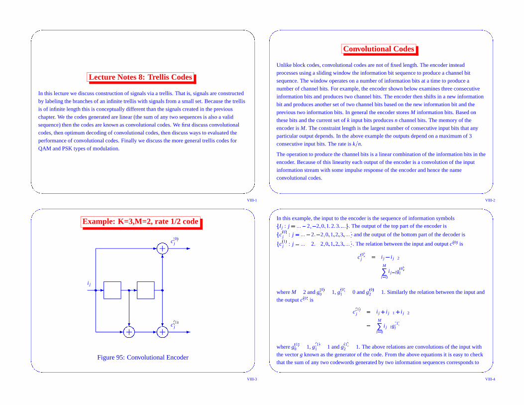
The operation of the encoder can be determined completely by way of a state transition

diagram. The state transition diagram is a directed graph with nodes for each possible encoder

content and transition between nodes corresponding to the results of different input bits to the

encoder. The transitions are labeled with the output bits of the code. This is shown for the

previous example.

VIII-5

��

��

01

11

00

10

1/11

0/00

1/100/10

0/01

1/00

0/11

1/01

i j �� c� 0

j � c� 1

j �

Figure 96: State Transition Diagram of Encoder

VIII-6

��

��

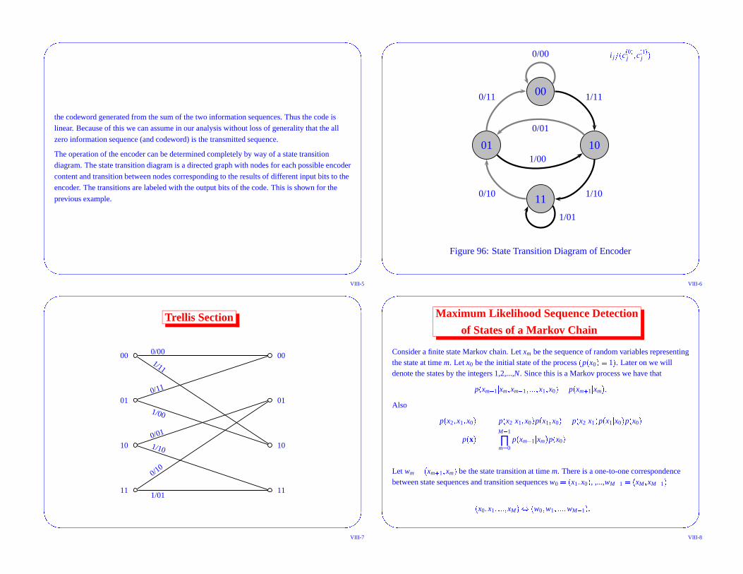
Trellis Section

00

01

10

11

00

01

10

11

0/001/11

1/00

0/11

0/01

1/10

0/10

1/01

VIII-7

��

��

Maximum Likelihood Sequence Detection

of States of a Markov Chain

Consider a finite state Markov chain. Let xm be the sequence of random variables representingthe state at time m. Let x0 be the initial state of the process� p� x0 � � 1 � . Later on we willdenote the states by the integers 1,2,...,N. Since this is a Markov process we have that

p� xm � 1 � xm � xm� 1 � � � � � x1 � x0 � � p� xm � 1 � xm � �

Also

p� x2 � x1 � x0 � � p� x2 � x1 � x0 � p� x1 � x0 � � p� x2 � x1 � p� x1 � x0 � p� x0 �

p� x � � M� 1

∏m� 0

p� xm � 1 � xm � p� x0 �

Let wm� � xm � 1 � xm � be the state transition at time m. There is a one-to-one correspondencebetween state sequences and transition sequences w0� � x1 � x0 � , ,...,wM� 1� � xM � xM� 1 �

� x0 � x1 � � � � � xM �� � w0 � w1 � � � � � wM� 1 � �

VIII-8

��

��

Observation

By some mechanism (e.g. a noisy channel) a noisy version � zm � of the state transition

sequence is observed. Based on this noisy version of � wm � we wish to estimate the state

sequence � xm � or the transition sequence � wm � . Since � wm � and � xm � contain the same

information we have that

p� z � x � � p� z � w �

where z� z0 � z1 � � � � � zM� 1, x� x0 � x1 � � � � � xM, and w� w0 � � � � � wM� 1. We say a channel is

memoryless if

p� z � w � � M� 1

∏m� 0

p� zm � wm �

VIII-9

��

��

Likelihood Calcluation

So given an observation z on a memoryless channel our goal is to find the state sequence x for

which the aposteriori probability p� x � z � is largest. This minimizes the probability that we

choose the wrong sequence. Thus the optimum (minimum sequence error probability)

decoder chooses x which maximizes p� x � z � : i.e

x̂ � argmaxx p� x � z �� argmaxx p� x � z �� argminx � � log p� x � z � �� argminx � � log p� z � x � p� x � �

VIII-10

��

��

Markov State and Memoryless Channel

Using the memoryless property of the channel we obtain

p� z � x � � M� 1

∏m� 0

p� zk � wm � �

Using the Markov property of the state sequence (with given initial state) yields

p� x � � M� 1

∏m� 0

p� xm � 1 � xm �

Define λ� wm � as follows:

λ� wm � � � ln p� xm � 1 � xm � � ln p� zm � wm �

Then

x̂� argminx � M� 1

∑m� 0

λ� wm � �

This problem formulation leads to a recursive solution. The recursive solution is called the

Viterbi Algorithm by communication engineers and is a form of dynamic programming as

studied by control engineers. They are really the same though.

VIII-11

��

��

Viterbi algorithm (dynamic programming)

Let Γ� xm � be the length (optimization criteria) of the shortest (optimum) path to state xm attime m. Let x̂� xm � be the shortest path to state xm at time m. Let Γ̂� xm � 1 � xm � be the length ofthe path to state xm � 1 at time m that goes through state xm at time m.

Then the algorithm works as follows.

Storage:

m, time index,

x̂� xm � � xm� � 1 � 2 � � � � � M �

Γ� xm � � xm� � 1 � 2 � � � � � M �Initialization

m� 0,

x̂� x0 � � x0

x̂� xm � arbitrary, m �� x0

Γ� x0 � � 0

Γ� m � � ∞, m �� ∞

VIII-12

��

��

Recursion

Γ̂� xm � 1 � xm � � Γ� xm � � λ� wm �

Γ� xm � 1 � � minxm Γ̂� xm � 1 � xm � for each xm � 1

Let x̂m� xm � 1 � � argminxmΓ̂� xm � 1 � xm � . x̂� xm � 1 � � � x̂� xm � � xm � 1 �

Justification:

Basically we are interested in finding the shortest length path through the trellis. At time m we

find the shortest length paths to each of the possible states at time m by computing all possible

ways of getting to state xm� u from a state at time m� 1. If the shortest path (denoted by

x̂� u � ) to get to xm� u at time m goes through state xm� 1� v at time m� 1 (i.e. x̂� u � � x̂� v � � u)

then the corresponding path x̂� v � to state xm� 1� v must be the shortest path to state v at time

m� 1 since if there was a shorter path, say x̃� v � , to state v at time m� 1 then the path x̃� v � � u to

state u at time m that used this shorter path to state v at time m� 1 would be shorter then what

we assumed was the shortest path). Stated another way if the shortest way of getting to state u

at time m is by going through state v at time m� 1 then the path used to get to state v at time

m� 1 must be the shortest of all paths to state v at time m� 1.

VIII-13

��

��

We identify a state transition with the pair of bits transmitted. The received pair of decision

statistics is our noisy information about the transition. Thus p� z � w � in this case is just the

transition probabilities from the input of the channel to the output of the channel. This is

because knowing the state transition determines the channel input.

VIII-14

��

��

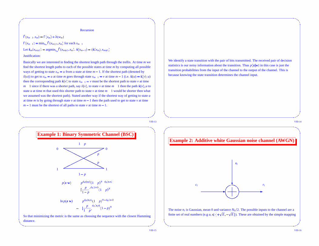
Example 1: Binary Symmetric Channel (BSC)

� � � � � � � � � � � �� � � � � � � � � � � �1 1

0 0

1� p

1� p

p

p

p� z � w � � pdH� z � c � 1� p �

N� dH� z � c

� � p1� p� dH� z � c

� 1� p �

N

ln p� z � w � � pdH� z � c � 1� p �

N� dH� z � c

� � p1� p� dH� z � c

� 1� p �

N

So that minimizing the metric is the same as choosing the sequence with the closest Hammingdistance.

VIII-15

��

��

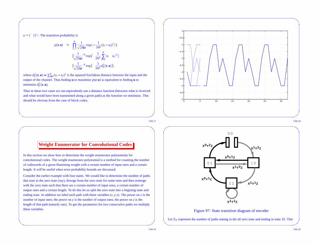
Example 2: Additive white Gaussian noise channel (AWGN)

�����

��

ci

ni

ri

The noise ni is Gaussian, mean 0 and variance N0 � 2. The possible inputs to the channel are a

finite set of real numbers (e.g ui� � � E �� E � ). These are obtained by the simple mapping

VIII-16

��

��

u� � � 1 �c j . The transition probability is

p� z � u � � N

∏i� 1

1 2πσexp � � 1

2σ2� zi� ui �

2 � �

� � 1 2πσ� N exp � � 12σ2

N

∑i� 1

� zi� ui �

2 �

� � 1 2πσ� N exp � � 12σ2 d2

E� z � u � � �

where d2E� z � u � � ∑N

i� 1� zi� ui �

2 is the squared Euclidean distance between the input and the

output of the channel. Thus finding u to maximize p� z � u � is equivalent to finding u to

minimize d2E� z � u � .

Thus in these two cases we can equivalently use a distance function (between what is received

and what would have been transmitted along a given path) as the function we minimize. This

should be obvious from the case of block codes.

VIII-17

��

��

0 5 10 15 20 25 30−5

−4.5

−4

−3.5

−3

−2.5

−2

−1.5

−1

−0.5

0

VIII-18

��

��

Weight Enumerator for Convolutional Codes

In this section we show how to determine the weight enumerator polynomials for

convolutional codes. The weight enumerator polynomial is a method for counting the number

of codewords of a given Hamming weight with a certain number of input ones and a certain

length. It will be useful when error probability bounds are discussed.

Consider the earlier example with four states. We would like to determine the number of paths

that start in the zero state (say), diverge from the zero state for some time and then remerge

with the zero state such that there are a certain number of input ones, a certain number of

output ones and a certain length. To do this let us split the zero state into a begining state and

ending state. In addition we label each path with three variables (x � y � z). The power on x is the

number of input ones; the power on y is the number of output ones; the power on z is the

length of that path (namely one). To get the parameters for two consecutive paths we multiply

these variables.

VIII-19

��

��

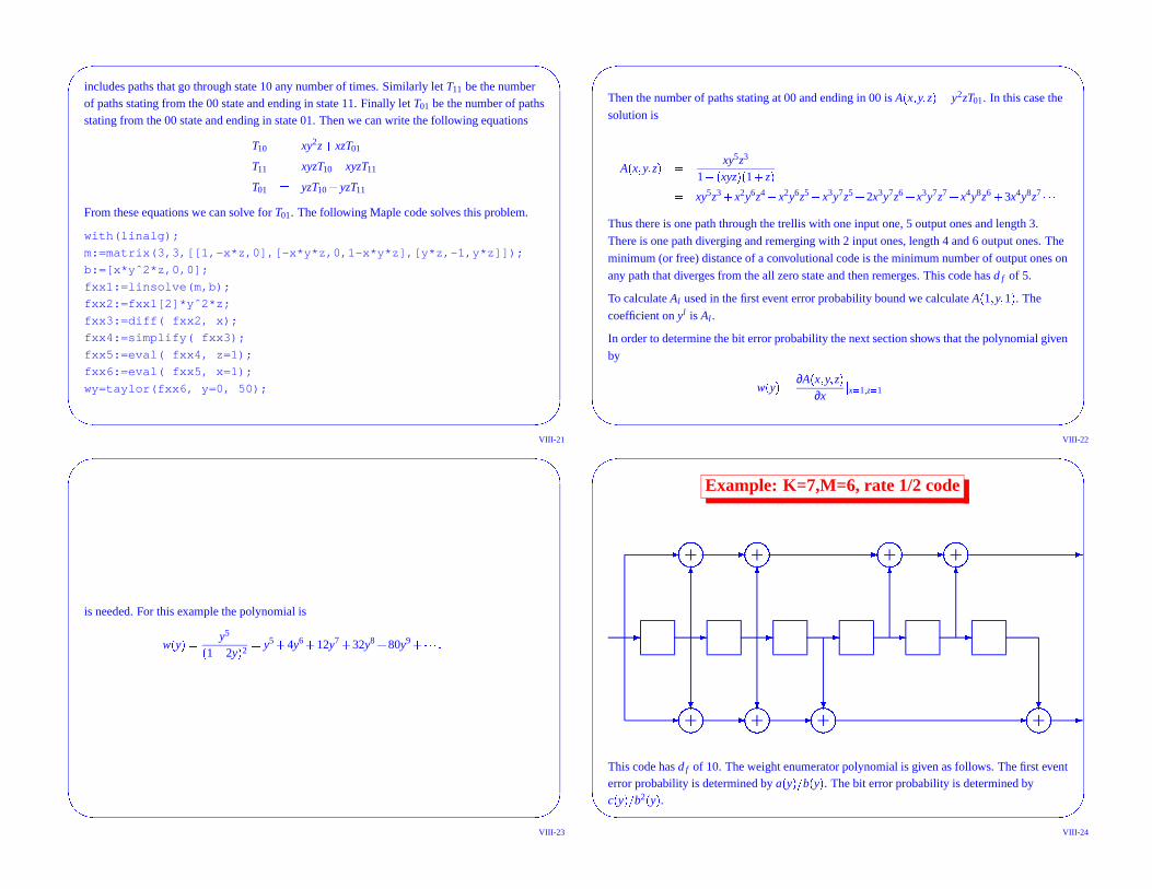
1001

11

00

X1Y1Z

X0Y1Z

X0Y2Z

X0Y1Z

X1Y0Z

X1Y2Z

X1Y1Z

Figure 97: State transition diagram of encoder

Let T10 represent the number of paths stating in the all zero state and ending in state 10. This

VIII-20

��

��

includes paths that go through state 10 any number of times. Similarly let T11 be the numberof paths stating from the 00 state and ending in state 11. Finally let T01 be the number of pathsstating from the 00 state and ending in state 01. Then we can write the following equations

T10 � xy2z� xzT01

T11 � xyzT10� xyzT11

T01 � yzT10� yzT11

From these equations we can solve for T01. The following Maple code solves this problem.

with(linalg);

m:=matrix(3,3,[[1,-x*z,0],[-x*y*z,0,1-x*y*z],[y*z,-1,y*z]]);

b:=[x*yˆ2*z,0,0];

fxx1:=linsolve(m,b);

fxx2:=fxx1[2]*yˆ2*z;

fxx3:=diff( fxx2, x);

fxx4:=simplify( fxx3);

fxx5:=eval( fxx4, z=1);

fxx6:=eval( fxx5, x=1);

wy=taylor(fxx6, y=0, 50);

VIII-21

��

��

Then the number of paths stating at 00 and ending in 00 is A� x � y � z � � y2zT01. In this case the

solution is

A� x � y � z � � xy5z3

1� � xyz �� 1� z �� xy5z3� x2y6z4� x2y6z5� x3y7z5� 2x3y7z6� x3y7z7� x4y8z6� 3x4y8z7

� � �

Thus there is one path through the trellis with one input one, 5 output ones and length 3.

There is one path diverging and remerging with 2 input ones, length 4 and 6 output ones. The

minimum (or free) distance of a convolutional code is the minimum number of output ones on

any path that diverges from the all zero state and then remerges. This code has d f of 5.

To calculate Al used in the first event error probability bound we calculate A� 1 � y � 1 � . The

coefficient on yl is Al .

In order to determine the bit error probability the next section shows that the polynomial given

by

w� y � � ∂A� x � y � z �

∂x � x� 1 � z� 1�

VIII-22

��

��

is needed. For this example the polynomial is

w� y � � y5

� 1� 2y �

2

� y5� 4y6� 12y7� 32y8� 80y9� � � � �

VIII-23

��

��

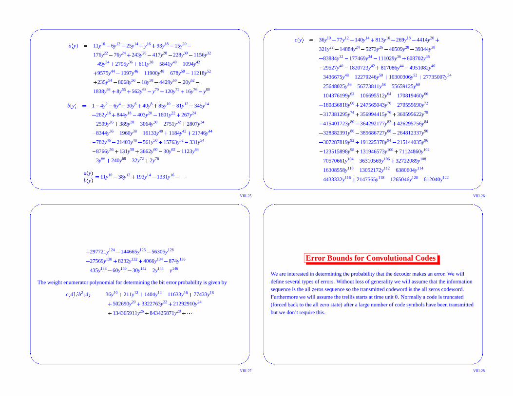
Example: K=7,M=6, rate 1/2 code

� � � � � �

�� ��� �� � � � �� ��� �� ��� �

� ���� � �� � � � �� � � � ���� �

This code has d f of 10. The weight enumerator polynomial is given as follows. The first eventerror probability is determined by a� y � � b� y � . The bit error probability is determined byc� y � � b2

� y � .

VIII-24

��

��

a� y � � 11y10� 6y12� 25y14� y16� 93y18� 15y20�

176y22� 76y24� 243y26� 417y28� 228y30� 1156y32

� 49y34� 2795y36� 611y38� 5841y40� 1094y42

� 9575y44� 1097y46� 11900y48� 678y50� 11218y52

� 235y54� 8068y56� 18y58� 4429y60� 20y62�

1838y64� 8y66� 562y68� y70� 120y72� 16y76� y80

b� y � � 1� 4y2� 6y4� 30y6� 40y8� 85y10� 81y12� 345y14

� 262y16� 844y18� 403y20� 1601y22� 267y24

� 2509y26� 389y28� 3064y30� 2751y32� 2807y34

� 8344y36� 1960y38� 16133y40� 1184y42� 21746y44

� 782y46� 21403y48� 561y50� 15763y52� 331y54

� 8766y56� 131y58� 3662y60� 30y62� 1123y64

� 3y66� 240y68� 32y72� 2y76

a� y �

b� y �� 11y10� 38y12� 193y14� 1331y16� � � �

VIII-25

��

��

c� y � � 36y10� 77y12� 140y14� 813y16� 269y18� 4414y20�

321y22� 14884y24� 5273y26� 40509y28� 39344y30

� 83884y32� 177469y34� 111029y36� 608702y38

� 29527y40� 1820723y42� 817086y44� 4951082y46

� 3436675y48� 12279246y50� 10300306y52� 27735007y54

� 25648025y56� 56773811y58� 55659125y60

� 104376199y62� 106695512y64� 170819460y66

� 180836818y68� 247565043y70� 270555690y72

� 317381295y74� 356994415y76� 360595622y78

� 415401723y80� 364292177y82� 426295756y84

� 328382391y86� 385686727y88� 264812337y90

� 307287819y92� 191225378y94� 215144035y96

� 123515898y98� 131946573y100� 71124860y102

� 70570661y104� 36310569y106� 32722089y108

� 16308558y110� 13052172y112� 6380604y114

� 4433332y116� 2147565y118� 1265046y120� 612040y122

VIII-26

��

��

� 297721y124� 144665y126� 56305y128

� 27569y130� 8232y132� 4066y134� 874y136

� 435y138� 60y140� 30y142� 2y144� y146

The weight enumerator polynomial for determining the bit error probability is given by

c� d � � b2

� d � � 36y10� 211y12� 1404y14� 11633y16� 77433y18

� 502690y20� 3322763y22� 21292910y24

� 134365911y26� 843425871y28� � � �

VIII-27

��

��

Error Bounds for Convolutional Codes

We are interested in determining the probability that the decoder makes an error. We will

define several types of errors. Without loss of generality we will assume that the information

sequence is the all zeros sequence so the transmitted codeword is the all zeros codeword.

Furthermore we will assume the trellis starts at time unit 0. Normally a code is truncated

(forced back to the all zero state) after a large number of code symbols have been transmitted

but we don’t require this.

VIII-28

��

��

First Event Error

A first event error is said to occur at time m if the all zeros path (correct path) is eliminated for

the first time at time m, that is, if the path with the shortest distance to the 0 state at time m is

not the all zeros path and this is the first time that the all zero path has been eliminated. At

time m an incorrect path will be chosen over the correct path if

P � incorrect path � received sequence � is greater than P � correct path � received sequence � . If the

incorrect path has (output) weight d then the probability that the incorrect path being more

likely than the all zeros path is denoted as P2� d � . This is easily calculated for most channels

since it is just the error probability of a repetition code of length d. For an additive white

Gaussian channel it is given by

P2� d � � Q� � 2Ed � N0 �

For a binary symmetric channel with crossover probability p it is given by

P2� d � � ��

�

∑dn� � d � 1 � 2 � d

n� pn

� 1� p �

d� n d odd

∑dn� d� 2 � 1 � d

n� pn

� 1� p �

d� n� 12 � d

d� 2� pd� 2� 1� p �

d� 2 d even

The first event error probability at time m, Pf � m, can then be bounded (using the union bound)

VIII-29

��

��

as

Pf � m� E ��

∞

∑l� 0

AlP2� l �

where Al is the number of paths through the trellis with output weight l. This is a union type

bound. However, it is also an upper bound since at any finite time m there will only be a finite

number of incorrect paths that merge with the correct path at time m. We have included in the

upper bound paths of all lengths as if the trellis started at t� � ∞. This makes the bound

independent of the time index j. (We will show later how to calculate Al for all l via a

generating function).

Since each term in the infinite sum is nonnegative, the sum is either a finite positive number or

∞. For example the standard code of constraint length 3 has Al� 2l� 5 so unless the pairwise

error probability decreases faster than 2� l the above bound will be infinite. The pairwise error

probability will decrease fast enough for reasonably large signal-to-noise ratio or reasonably

small crossover probability. In general the sequence � Al � may have a periodic component that

is zero but otherwise is a positive increasing sequence. P2� l � for reasonable channels is a

decreasing sequence. If the channel is fairly noisy then the above upper bound on first event

error probability may converge to something larger than 1, even ∞. In this case clearly 1 is an

VIII-30

��

��

upper bound on any probability we are interested in, so the above bound can be “improved” to

Pf � m� E �� min � 1 � ∞

∑l� 0

AlP2� l � � �

For example, the well known constraint length 7, rate 1/2 convolutional code has coefficients

that grow no faster than� 2 � 3876225 �

k so that provided P2� l � decreases faster than

� 2 � 3876225 �� k the bound above will converge. Since P2� l � � Dl where (for hard decisions)

D� 2 � p� 1� p � the above bound converges for p� 0 � 046. For soft decisions (and additive

white Gaussian noise) D� e� E� N0 and thus the bound converges provided E � N0� � 0 � 6dB.

VIII-31

��

��

Bit error probability

Below we find an upper bound on the error probability for binary convolutional codes. Thegeneralization to nonbinary codes is straightforward.

In order to calculate the bit error probability in decoding between time m and m� 1 we needto consider all paths through the trellis that are not in the all zeros state at either time unit m orm� 1. We also need to realize that not all incorrect paths will cause an error. First consider arate 1 � n code (i.e. k� 1) so each transition from one state to the next is determined by asingle bit. To compute an upper bound on the bit error probability we will do a union boundon all paths that cause a bit error. We assume that the trellis started at t� � ∞. We do this intwo steps. First we look at each path diverging and then remerging to the all zero state. This iscalled an error event. (An error event can only diverge once from the all zero state). Then sumover all possible starting times (times when the path diverges from the all zero state) for eachof these error events. So take a particular error event of length l corresponding to a statesequence with i input ones and j output ones and let Ai � j � l be the number of such paths. If theerror event started at time unit m then that clearly would cause an error since the input bitneed be one upon starting an error event (diverging from the all zero state). However, if theevent ended at time unit m� 1 in the all zero state then there would not be a bit error madesince remerging to the all zero state corresponds to an input bit of 0. Of the l phases that

VIII-32

��

��

overlap with the transition from m to m� 1 there are exactly i of these that will cause a biterror. So for each error event we need to weight the probability by the number of input onesthat are on that path. Thus the bit error probability (for k� 1) can be upper bounded by

Pb� ∑i � j � l iAi � j � lP2� j �

where P2� j � is the probability of error between two codewords that differ in j positions. Asbefore, this bound is independent of the time index m since we have included all paths as ifthe trellis started at t� � ∞ and goes on to t� � ∞.

If we define the weight enumerator polynomial for a convolutional code as

A� x � y � z � � ∑i � j � l Ai � j � lxiy jzl

and upper bound P2� j � using the Chernoff or Bhattacharyya bound by D j then the upperbound on first event error probability is just

Pf� E � � A� x � y � z � � x� 1 � y� D � z� 1

Similarly the bit error probability can be further upper bounded by

Pb�

∂A� x � y � z �

∂x � x� 1 � y� D � z� 1

VIII-33

��

��

As mentioned previously the above bounds may be larger than one (for small signal-to-noise

ratio or high cross over probability). This will happen for a larger range of parameters when

we use the generating function with the Bhattacharyya bound as opposed to just the union

bound. There is a way for certain codes to use just the union bound for the first say L terms

and the Bhattacharyya bound for remaining to get a tighter bound than the bound based on the

generating function but without the infinite computation required for just the union bound.

(See some problem). The above bounds only are finite for a certain range of the parameter D

depending on the specific code. However for practical codes and reasonable signal-to-noise

ratios or crossover probabilities the above bounds are finite. (See another problem).

VIII-34

��

��

Rate k � n codes

Now consider a rate k � n convolutional code. The trellis for such a code has 2k branchesemerging from each state. We will consider the bit error probability for the r-th bit in each k

bit input sequence. Let Ai1 �� � � � ik � j � l be the number of paths through the trellis with j outputones, length l, ir input ones in the r-th input bit (1� r� k) of the sequence of k bit inputs.Then clearly

Ai � j � l� ∑i1 �� � � � ik :∑k

r� 1 ir� i

Ai1 �� � � � ik � j � lThe bit error probability for the r-th bit is then bounded by

Pb � r� ∑i1 �� � � � ik � j � l irAi1 �� � � � ik � j � lP2� j �

The average bit error probability is

Pb� 1k

k

∑r� 1

Pb � r� 1k

k

∑r� 1

∑i1 �� � � � ik � j � l irAi1 �� � � � ik � j � lP2� j �

Pb�

1k ∑

j � l P2� j � ∑i1 �� � � � ik

k

∑r� 1

irAi1 �� � � � ik � j � lVIII-35

��

��

Pb�

1k ∑

j � l P2� j � ∑i1 �� � � � ik Ai1 �� � � � ik � j � l k

∑r� 1

ir

Now consider the last two sums.

∑i1 �� � � � ik�

k

∑r� 1

ir � Ai1 �� � � � ik � j � l � ∑i

∑i1 �� � � � ik :∑ ir� i

�

k

∑r� 1

ir � Ai1 �� � � � ik � j � l

� ∑i

∑i1 �� � � � ik :∑ ir� i

� i � Ai1 �� � � � ik � j � l

� ∑i

i ∑i1 �� � � � ik :∑ ir� i

Ai1 �� � � � ik � j � l

� ∑i

iAi � j � lThus

Pb�

1k ∑

i � j � l iAi � j � lP2� j � �

We can write this as

Pb�

1k ∑

j

w jP2� j � �VIII-36

��

��

where

w j� ∑i � l iAi � j � l

VIII-37

��

��

Improved Union-Bhattacharrya Bound

We can upper bound the bit error probability by

Pb� ∑j

w jP2� j �� ∑j

w jDj� w� D �

The first bound is the union bound. It is impossible to exactly evaluate this bound because

there are an infinite number of terms in the summation. Dropping all but the first N terms

gives an approximation. It may no longer be an upper bound though. If the weight enumerator

is known we can get arbitrarily close to the union bound and still get a bound as follows.

Pb � ∑j

w jP2� j � � N

∑j� d f

w jP2� j � � ∞

∑j� N � 1

w jP2� j �

�

N

∑j� d f

w jP2� j � � ∞

∑j� N � 1

w jDj

� N

∑j� d f

w j� P2� j � � D j

� � ∞

∑j� d f

w jDj

VIII-38

��

��

� N

∑j� d f

w j� P2� j � � D j

� � w� D �

The second term is the Union-Bhattacharyya (U-B) bound. The first term is clearly less than

zero, so we get something that is tighter than the U-B bound. By chosing N sufficiently large

we can sometimes get significant improvements over the U-B bound. Below we show the

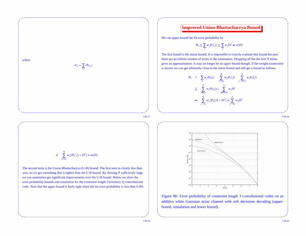
error probability bounds and simulation for the constraint length 3 (memory 2) convolutional

code. Note that the upper bound is fiarly tight when the bit error probability is less than 0.001.

VIII-39

��

��

0 1 2 3 4 5 6 7 810

−8

10−7

10−6

10−5

10−4

10−3

10−2

10−1

100

Eb/N0B

it E

rror

Rat

e

Upper bound

Simulation

Lower bound

Figure 98: Error probability of constraint length 3 convolutional codes on anadditive white Gaussian noise channel with soft decisions decoding (upper-bound, simulation and lower bound).

VIII-40

��

��

0 1 2 3 4 5 610

−6

10−5

10−4

10−3

10−2

10−1

100

Eb/N

0

Pb

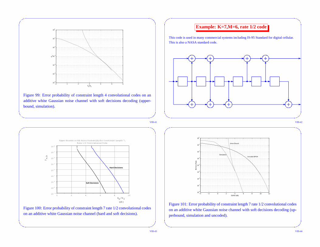
Figure 99: Error probability of constraint length 4 convolutional codes on anadditive white Gaussian noise channel with soft decisions decoding (upper-bound, simulation).

VIII-41

��

��

Example: K=7,M=6, rate 1/2 code

This code is used in many commercial systems including IS-95 Standard for digital cellular.

This is also a NASA standard code.

� � � � � �

�� ��� �� � � � �� ��� �� ��� �

� ���� � �� � � � �� � � � ���� �

� � � � � �

VIII-42

��

��

108642010 -10

10 -9

10 -8

10 -7

10 -6

10 -5

10 -4

10 -3

10 -2

U pper Bounds on Bit Error Probabilityfor Constraint Length 7,

R ate 1/2 Convolutional Code

Eb/N0

(dB)

Pe,b

Hard Decisions

Soft Decisions

Figure 100: Error probability of constraint length 7 rate 1/2 convolutional codeson an additive white Gaussian noise channel (hard and soft decisions).

VIII-43

��

��

−4 −2 0 2 4 6 8 10 1210

−8

10−7

10−6

10−5

10−4

10−3

10−2

10−1

100

Eb/N0 (dB)B

it E

rror

Rat

e

Simulation

Union Bound

Uncoded BPSK

Figure 101: Error probability of constraint length 7 rate 1/2 convolutional codeson an additive white Gaussian noise channel with soft decisions decoding (up-perbound, simulation and uncoded).

VIII-44

��

��

Bit Error Probability (Bound) for Constraint Length 9 Rate 1/3 Convolutional Code

Eb/N 0 (dB)

Bit Error Probability

108642010 -10

10 -9

10 -8

10 -7

10 -6

10 -5

10 -4

10 -3

10 -2

10 -1

10 0

Hard Decisions

Soft Decisions

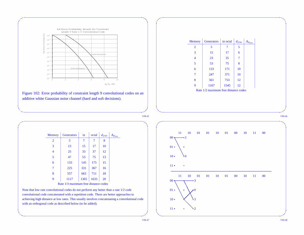
Figure 102: Error probability of constraint length 9 convolutional codes on anadditive white Gaussian noise channel (hard and soft decisions).

VIII-45

��

��

Memory Generators in octal d f ree Ad f ree

2 5 7 5

3 15 17 6

4 23 35 7

5 53 75 8

6 133 171 10

7 247 371 10

8 561 753 12

9 1167 1545 12

Rate 1/2 maximum free distance codes

VIII-46

��

��

Memory Generators in octal d f ree Ad f ree

2 5 7 7 8

3 13 15 17 10

4 25 33 37 12

5 47 53 75 13

6 133 145 175 15

7 225 331 367 16

8 557 663 711 18

9 1117 1365 1633 20

Rate 1/3 maximum free distance codes

Note that low rate convolutional codes do not perform any better than a rate 1/2 code

convolutional code concatenated with a repetition code. There are better approaches to

achieving high distance at low rates. This usually involves concatenating a convolutional code

with an orthogonal code as described below (to be added).

VIII-47

��

��

11 10 01 01 10 01 00 10 11 00

��

��

��

��

11

10

01

00

��

��

��

2

0

11 10 01 01 10 01 00 10 11 00�

��

�

��

��

��

��

11

10

01

00

��

��

�� �

��

��

�

��

��

��

2

3

0

3

VIII-48

��

��

11 10 01 01 10 01 00 10 11 00

��

��

��

��

��

��

��

��

11

10

01

00�

��

��

� ��

�

��

�

��

��

��

��

��

��

��

�

��

�

��

�3

1

2

1

11 10 01 01 10 01 00 10 11 00

��

��

��

��

��

��

��

��

��

��

11

10

01

00

��

��

�� �

��

��

�

��

��

��

��

��

��

��

�

��

�

��

��

��

��

�

��

�

��

�

��

��

��

1

2

3

2

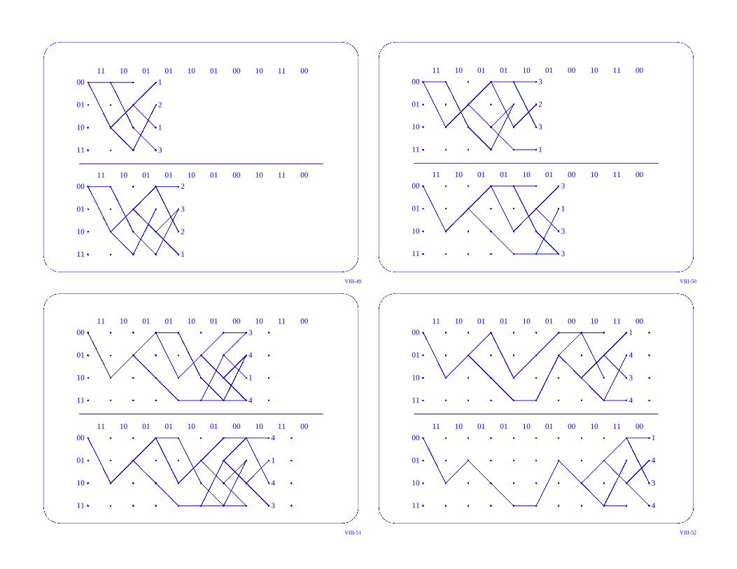
VIII-49

��

��

11 10 01 01 10 01 00 10 11 00

��

��

��

��

��

��

��

��

��

��

��

��

11

10

01

00

��

��

�� �

��

��

��

��

��

�

��

�

��

��

��

��

�

��

�

��

�

��

��

�� �

��

��

��

��

1

3

2

3

11 10 01 01 10 01 00 10 11 00

��

��

��

��

��

��

��

��

��

��

��

��

��

��

11

10

01

00

��

��

�� �

��

��

�

��

��

��

��

��

�� �

��

��

��

��

��

��

��

��

�

��

�

��

�

3

3

1

3

VIII-50

��

��

11 10 01 01 10 01 00 10 11 00

��

��

��

��

��

��

��

��

��

��

��

��

��

��

��

��

��

��

11

10

01

00

��

��

�� �

��

��

�

��

��

��

��

��

�� �

��

��

��

��

��

��

��

��

�

��

�

��

��

��

��

�

��

�

��

�

��

�

��

�

4

1

4

3

11 10 01 01 10 01 00 10 11 00

��

��

��

��

��

��

��

��

��

��

��

��

��

��

��

��

��

��

��

��

11

10

01

00

��

��

�� �

��

��

�

��

��

��

��

��

�� �

��

��

��

��

��

��

��

��

�

��

�

��

��

��

��

�

��

�

��

�

��

�

��

��

��

��

�

��

��

��

3

4

1

4

VIII-51

��

��

11 10 01 01 10 01 00 10 11 00

��

��

��

��

��

��

��

��

��

��

��

��

��

��

��

��

��

��

��

��

��

��

11

10

01

00

��

��

�� �

��

��

�

��

��

��

��

��

�� �

��

��

��

��

��

��

��

��

��

��

��

�

��

��

��

��

��

��

��

�

��

�

4

3

4

1

11 10 01 01 10 01 00 10 11 00�

��

�

��

��

��

��

��

��

��

��

��

��

��

��

��

��

��

��

��

��

��

��

11

10

01

00

��

��

�� �

�� �

��

��

� ��

��

�� �

��

��

�

��

��

��

��

�

��

�

��

� ��

�

��

�

��

��

��

4

3

4

1

VIII-52

��

��

Error Bounds for Convolutional Codes

The performance of convolutional codes can be upper bounded by

Pb�

∞

∑l� d f ree

wlDl

where wl is the average number of nonzero information bits on paths with Hamming distance

l and D is a parameter that depends only on the channel. usually the summation in the upper

bound is truncated to some finite number of terms. Example 1. Binary Symmetric Channel

crossover probability p.

D� 2 � p� 1� p �

Example 2. Additive White Gaussian Noise channel

D� e

� E� N0 �Performance Examples: Generally hard decisions requires 2dB more signal energy than soft

decisions for the same bit error probability. Also soft decisions is only about 0.25dB better

than 8 level quantization.

VIII-53

��

��

Standard codes:

Example Convolutional Code 1:

Constraint length 7, memory 6, 64 state decoder, rate 1/2 has the following upper bound.

Pb� 36D10� 211D12� 1404D14� 11633D16� � � �

There is a chip made by Qualcomm and Stanford Telecommunications that operates at data

rates on the order of 10Mbits/second that will do encoding and decoding.

Example Convolutional Code 2: Constraint length 9, memory 8, 256 state decoder, rate 1/2

Pb� 33D12� 281D14� 2179D16� 15035D18� � � �

Example Convolutional Code 3: Constraint length 9, memory 8, 256 state decoder, rate 1/3

Pb� 11D18� 32D20� 195D22� 564D24� 1473D26� � � �

VIII-54

��

��

Trellis

VIII-55

��

��

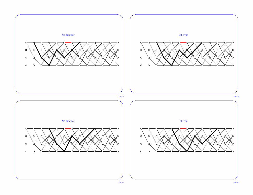
No bit error

VIII-56

��

��

No bit error

VIII-57

��

��

Bit error

VIII-58

��

��

No bit error

VIII-59

��

��

Bit error

VIII-60

��

��

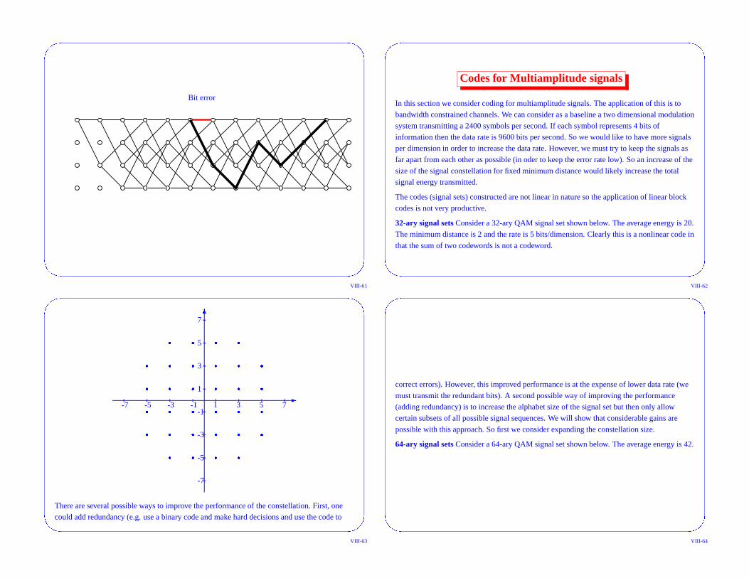
Bit error

VIII-61

��

��

Codes for Multiamplitude signals

In this section we consider coding for multiamplitude signals. The application of this is to

bandwidth constrained channels. We can consider as a baseline a two dimensional modulation

system transmitting a 2400 symbols per second. If each symbol represents 4 bits of

information then the data rate is 9600 bits per second. So we would like to have more signals

per dimension in order to increase the data rate. However, we must try to keep the signals as

far apart from each other as possible (in oder to keep the error rate low). So an increase of the

size of the signal constellation for fixed minimum distance would likely increase the total

signal energy transmitted.

The codes (signal sets) constructed are not linear in nature so the application of linear block

codes is not very productive.

32-ary signal sets Consider a 32-ary QAM signal set shown below. The average energy is 20.

The minimum distance is 2 and the rate is 5 bits/dimension. Clearly this is a nonlinear code in

that the sum of two codewords is not a codeword.

VIII-62

��

��

�

�� � � �

� � � � � �

� � � � � �

� � � � � �

� � � � � �

� � � �

-7 -5 -3 -1 1 3 5 7

-7

-5

-3

-1

1

3

5

7

There are several possible ways to improve the performance of the constellation. First, one

could add redundancy (e.g. use a binary code and make hard decisions and use the code to

VIII-63

��

��

correct errors). However, this improved performance is at the expense of lower data rate (we

must transmit the redundant bits). A second possible way of improving the performance

(adding redundancy) is to increase the alphabet size of the signal set but then only allow

certain subsets of all possible signal sequences. We will show that considerable gains are

possible with this approach. So first we consider expanding the constellation size.

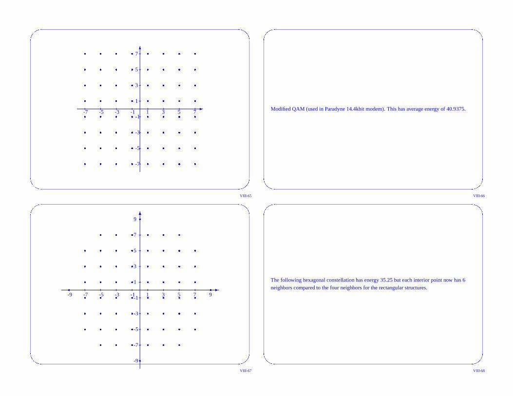
64-ary signal sets Consider a 64-ary QAM signal set shown below. The average energy is 42.

VIII-64

��

��

�

�

� � � � � � � �

� � � � � � � �

� � � � � � � �

� � � � � � � �

� � � � � � � �

� � � � � � � �

� � � � � � � �

� � � � � � � �

-7 -5 -3 -1 1 3 5 7

-7

-5

-3

-1

1

3

5

7

VIII-65

��

��

Modified QAM (used in Paradyne 14.4kbit modem). This has average energy of 40.9375.

VIII-66

��

��

�

�

� � � � � �

� � � � � � � �

� � � � � � � �

� � � � � � � �

� � � � � � � �

� � � � � � � �

� � � � � � � �

� � � � � �

� �

��

-9 -7 -5 -3 -1 1 3 5 7 9

-9

-7

-5

-3

-1

1

3

5

7

9

VIII-67

��

��

The following hexagonal constellation has energy 35.25 but each interior point now has 6

neighbors compared to the four neighbors for the rectangular structures.

VIII-68

��

��

�

�

�

�

�

�

�

�

�

�

�

�

�

�

�

�

�

�

�

�

�

�

�

�

�

�

�

�

�

�

�

�

�

�

�

�

�

�

�

�

�

�

�

�

�

�

�

�

�

�

�

�

�

�

�

�

�

�

�

�

�

�

�

�

�

�

-7 -5 -3 -1 1 3 5 7

-7

-5

-3

-1

1

3

5

7

VIII-69

��

��

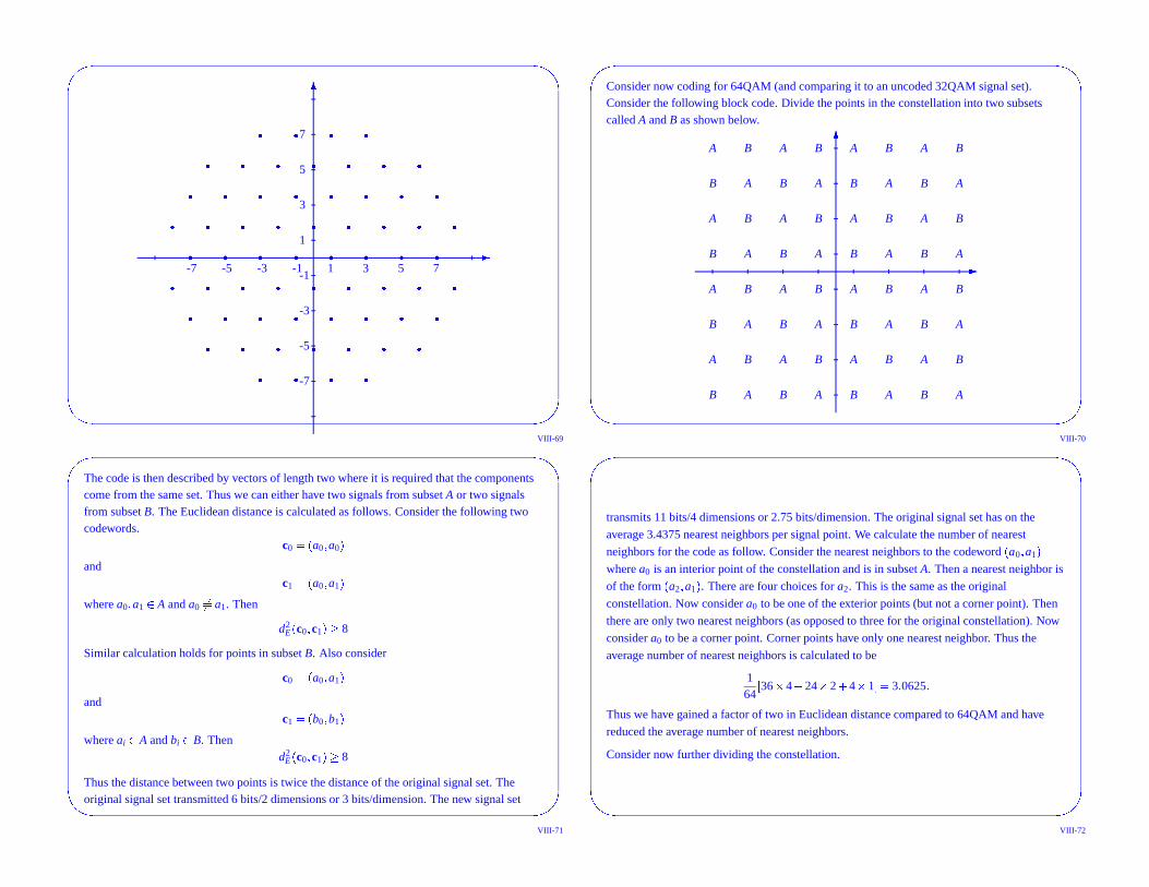
Consider now coding for 64QAM (and comparing it to an uncoded 32QAM signal set).Consider the following block code. Divide the points in the constellation into two subsetscalled A and B as shown below.

�

�

B B B BA A A A

A A A AB B B B

B B B BA A A A

A A A AB B B B

B B B BA A A A

A A A AB B B B

B B B BA A A A

A A A AB B B B

VIII-70

��

��

The code is then described by vectors of length two where it is required that the componentscome from the same set. Thus we can either have two signals from subset A or two signalsfrom subset B. The Euclidean distance is calculated as follows. Consider the following twocodewords.

c0� � a0 � a0 �

andc1� � a0 � a1 �

where a0 � a1� A and a0 �� a1. Then

d2E� c0 � c1 �� 8

Similar calculation holds for points in subset B. Also consider

c0� � a0 � a1 �

andc1� � b0 � b1 �

where ai� A and bi� B. Thend2

E� c0 � c1 �� 8

Thus the distance between two points is twice the distance of the original signal set. Theoriginal signal set transmitted 6 bits/2 dimensions or 3 bits/dimension. The new signal set

VIII-71

��

��

transmits 11 bits/4 dimensions or 2.75 bits/dimension. The original signal set has on the

average 3.4375 nearest neighbors per signal point. We calculate the number of nearest

neighbors for the code as follow. Consider the nearest neighbors to the codeword� a0 � a1 �

where a0 is an interior point of the constellation and is in subset A. Then a nearest neighbor is

of the form� a2 � a1 � . There are four choices for a2. This is the same as the original

constellation. Now consider a0 to be one of the exterior points (but not a corner point). Then

there are only two nearest neighbors (as opposed to three for the original constellation). Now

consider a0 to be a corner point. Corner points have only one nearest neighbor. Thus the

average number of nearest neighbors is calculated to be

164 � 36 � 4� 24 � 2� 4 � 1� � 3 � 0625 �

Thus we have gained a factor of two in Euclidean distance compared to 64QAM and have

reduced the average number of nearest neighbors.

Consider now further dividing the constellation.

VIII-72

��

��

�

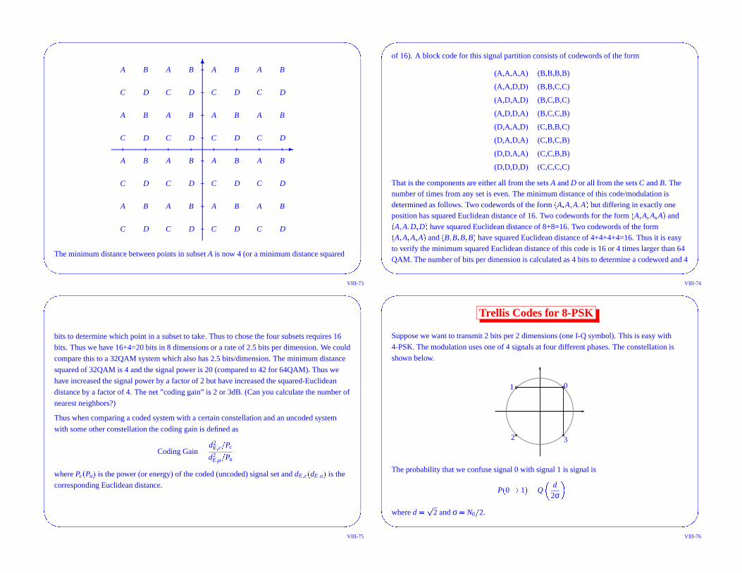
�C C C CD D D D

A A A AB B B B

C C C CD D D D

A A A AB B B B

C C C CD D D D

A A A AB B B B

C C C CD D D D

A A A AB B B B

The minimum distance between points in subset A is now 4 (or a minimum distance squared

VIII-73

��

��

of 16). A block code for this signal partition consists of codewords of the form

(A,A,A,A) (B,B,B,B)

(A,A,D,D) (B,B,C,C)

(A,D,A,D) (B,C,B,C)

(A,D,D,A) (B,C,C,B)

(D,A,A,D) (C,B,B,C)

(D,A,D,A) (C,B,C,B)

(D,D,A,A) (C,C,B,B)

(D,D,D,D) (C,C,C,C)

That is the components are either all from the sets A and D or all from the sets C and B. Thenumber of times from any set is even. The minimum distance of this code/modulation isdetermined as follows. Two codewords of the form� A � A � A � A � but differing in exactly oneposition has squared Euclidean distance of 16. Two codewords for the form� A � A � A � A � and

� A � A � D � D � have squared Euclidean distance of 8+8=16. Two codewords of the form

� A � A � A � A � and� B � B � B � B � have squared Euclidean distance of 4+4+4+4=16. Thus it is easyto verify the minimum squared Euclidean distance of this code is 16 or 4 times larger than 64QAM. The number of bits per dimension is calculated as 4 bits to determine a codeword and 4

VIII-74

��

��

bits to determine which point in a subset to take. Thus to chose the four subsets requires 16

bits. Thus we have 16+4=20 bits in 8 dimensions or a rate of 2.5 bits per dimension. We could

compare this to a 32QAM system which also has 2.5 bits/dimension. The minimum distance

squared of 32QAM is 4 and the signal power is 20 (compared to 42 for 64QAM). Thus we

have increased the signal power by a factor of 2 but have increased the squared-Euclidean

distance by a factor of 4. The net ”coding gain” is 2 or 3dB. (Can you calculate the number of

nearest neighbors?)

Thus when comparing a coded system with a certain constellation and an uncoded system

with some other constellation the coding gain is defined as

Coding Gain� d2E � c � Pc

d2E � u � Pu

where Pc� Pu � is the power (or energy) of the coded (uncoded) signal set and dE � c� dE � u � is the

corresponding Euclidean distance.

VIII-75

��

��

Trellis Codes for 8-PSK

Suppose we want to transmit 2 bits per 2 dimensions (one I-Q symbol). This is easy with

4-PSK. The modulation uses one of 4 signals at four different phases. The constellation is

shown below.

01

2 3

The probability that we confuse signal 0 with signal 1 is signal is

P� 0 � 1 � � Q

�

d2σ �

where d� 2 and σ� N0 � 2.

VIII-76

��

��

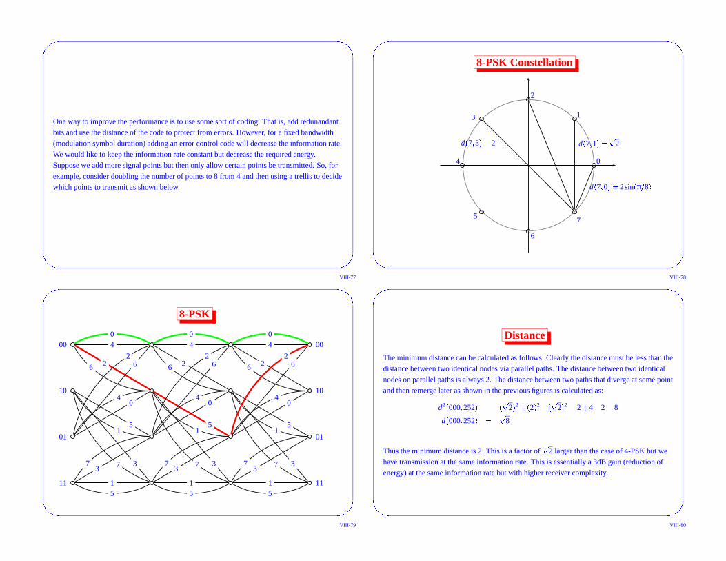
One way to improve the performance is to use some sort of coding. That is, add redunandant

bits and use the distance of the code to protect from errors. However, for a fixed bandwidth

(modulation symbol duration) adding an error control code will decrease the information rate.

We would like to keep the information rate constant but decrease the required energy.

Suppose we add more signal points but then only allow certain points be transmitted. So, for

example, consider doubling the number of points to 8 from 4 and then using a trellis to decide

which points to transmit as shown below.

VIII-77

��

��

8-PSK Constellation

d� 7 � 0 � � 2sin� π � 8 �

d� 7 � 1 � � 2d� 7 � 3 � � 2

0

1

2

3

4

5

6

7

VIII-78

��

��

8-PSK

00

10

01

11

00

10

01

11

40

26

51

37

62

04

37

15

40

26

51

37

62

04

37

15

40

26

51

37

62

04

37

15

VIII-79

��

��

Distance

The minimum distance can be calculated as follows. Clearly the distance must be less than the

distance between two identical nodes via parallel paths. The distance between two identical

nodes on parallel paths is always 2. The distance between two paths that diverge at some point

and then remerge later as shown in the previous figures is calculated as:

d2

� 000 � 252 � � � 2 �

2� � 2 �

2� � 2 �

2� 2� 4� 2� 8

d� 000 � 252 � � 8

Thus the minimum distance is 2. This is a factor of 2 larger than the case of 4-PSK but we

have transmission at the same information rate. This is essentially a 3dB gain (reduction of

energy) at the same information rate but with higher receiver complexity.

VIII-80

��

��

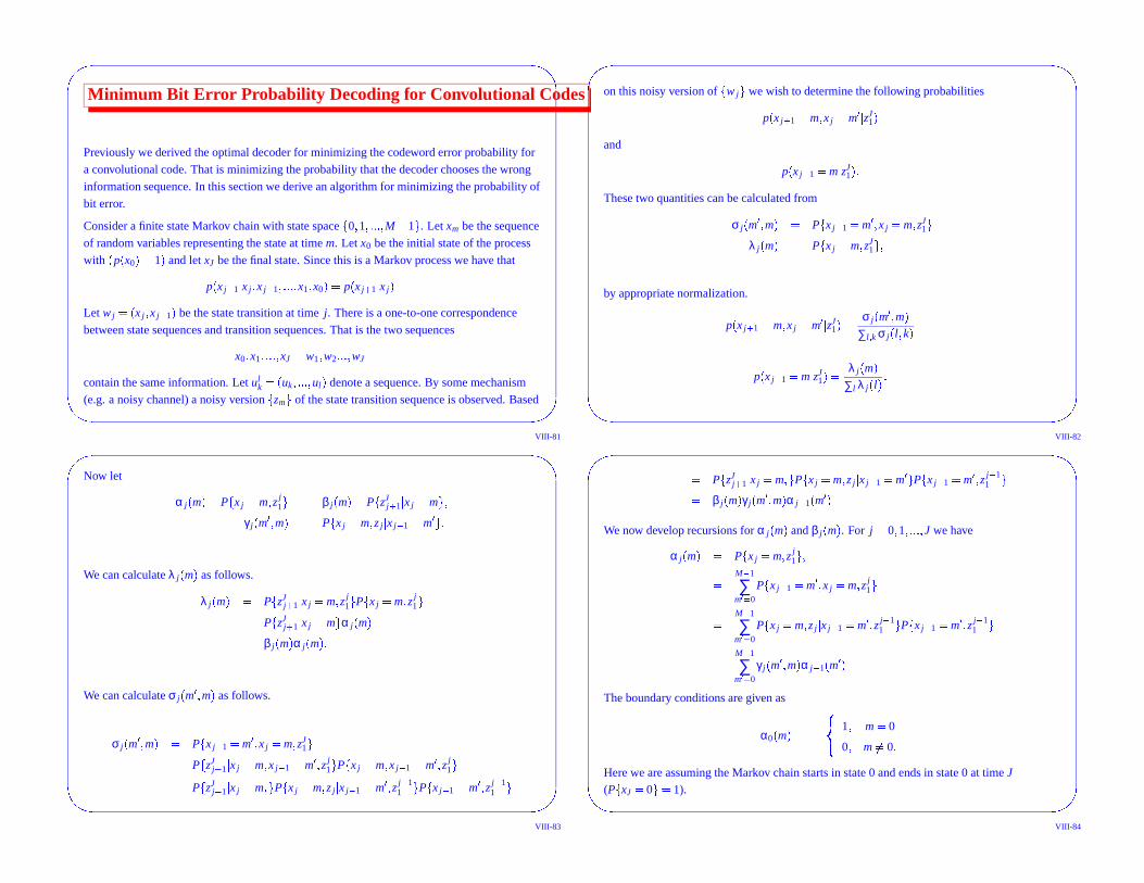
Minimum Bit Error Probability Decoding for Convolutional Codes

Previously we derived the optimal decoder for minimizing the codeword error probability for

a convolutional code. That is minimizing the probability that the decoder chooses the wrong

information sequence. In this section we derive an algorithm for minimizing the probability of

bit error.

Consider a finite state Markov chain with state space � 0 � 1 � � � � � M� 1 � . Let xm be the sequence

of random variables representing the state at time m. Let x0 be the initial state of the process

with� p� x0 � � 1 � and let xJ be the final state. Since this is a Markov process we have that

p� x j � 1 � x j � x j� 1 � � � � � x1 � x0 � � p� x j � 1 � x j �

Let w j� � x j � x j� 1 � be the state transition at time j. There is a one-to-one correspondence

between state sequences and transition sequences. That is the two sequences

x0 � x1 � � � � � xJ w1 � w2 � � � � wJ

contain the same information. Let ulk

� � uk � � � � � ul � denote a sequence. By some mechanism

(e.g. a noisy channel) a noisy version � zm � of the state transition sequence is observed. Based

VIII-81

��

��

on this noisy version of � w j � we wish to determine the following probabilities

p� x j � 1� m � x j� m� � zJ1 �

and

p� x j � 1� m � zJ1 � �

These two quantities can be calculated from

σ j� m� � m � � P � x j� 1� m� � x j� m � zJ1 �

λ j� m � � P � x j� m � zJ1 � �

by appropriate normalization.

p� x j � 1� m � x j� m� � zJ1 � � σ j� m� � m �

∑l � k σ j� l � k �

p� x j � 1� m � zJ1 � � λ j� m �

∑l λ j� l ��

VIII-82

��

��

Now let

α j� m � � P � x j� m � z j1 � β j� m � � P � zJ

j � 1 � x j� m � �

γ j� m� � m � � P � x j� m � z j � x j� 1� m� � �

We can calculate λ j� m � as follows.

λ j� m � � P � zJj � 1 � x j� m � z j

1 � P � x j� m � z j1 �� P � zJ

j � 1 � x j� m � α j� m �� β j� m � α j� m � �

We can calculate σ j� m� � m � as follows.

σ j� m� � m � � P � x j� 1� m� � x j� m � zJ1 �� P � zJ

j � 1 � x j� m � x j� 1� m� � z j1 � P � x j� m � x j� 1� m� � z j

1 �� P � zJj � 1 � x j� m � � P � x j� m � z j � x j� 1� m� � z j� 1

1 � P � x j� 1� m� � z j� 11 �

VIII-83

��

��

� P � zJj � 1 � x j� m � � P � x j� m � z j � x j� 1� m� � P � x j� 1� m� � z j� 1

1 �� β j� m � γ j� m� � m � α j� 1� m� �

We now develop recursions for α j� m � and β j� m � . For j� 0 � 1 � � � � � J we have

α j� m � � P � x j� m � z j1 � �

� M� 1

∑m �� 0

P � x j� 1� m� � x j� m � z j1 �

� M� 1

∑m �� 0

P � x j� m � z j � x j� 1� m� � z j� 11 � P � x j� 1� m� � z j� 1

1 �

� M� 1

∑m �� 0

γ j� m� � m � α j� 1� m� �

The boundary conditions are given as

α0� m � � ��

�

1 � m� 0

0 � m �� 0 �

Here we are assuming the Markov chain starts in state 0 and ends in state 0 at time J

(P � xJ� 0 � � 1).

VIII-84

��

��

The recursion for β j� m � is given as follows.

β j� m � � P � zJj � 1 � x j� m � �

� M� 1

∑m �� 0

P � x j � 1� m� � zJj � 1 � x j� m � �

� M� 1

∑m �� 0

P � zJj � 2 � x j � 1� m� � z j � 1 � x j� m � P � x j � 1� m� � z j � 1 � x j� m � �

� M� 1

∑m �� 0

P � zJj � 2 � x j � 1� m� � P � x j � 1� m� � z j � 1 � x j� m � �

� M� 1

∑m �� 0

β j � 1� m� � γ j � 1� m � m� � �The boundary condition is

βJ� m � � ��

�1 � m� 0

0 � m �� 0 �Finally we can calculate γ j� m� � m � as follows

γ j� m� � m � � P � x j� m � z j � x j� 1� m� �

VIII-85

��

��

� ∑w j

P � x j� m � z j � w j � x j� 1� m� �

� ∑w j

P � z j � x j� m � w j � x j� 1� m� � P � x j� m � w j � x j� 1� m� �

� ∑w j

P � z j � w j � P � w j � x j� m � x j� 1� m� � P � x j� m � x j� 1� m� �

The first term is the transition probability of the channel. The second term is the output of the

encoder when transitioning from state m to state m� . The last term is the probability of going

to state m from state m� . This will be either a nonzero constant (e.g. 1/2) or zero.

The algorithm works as follows. First initialize α and β. After receiving the vector z1 � � � � � zJ

perform the recursion on α and β. Then combine α and β to determine λ and σ. Normalize to

determine the desired probabilities.

VIII-86

��

��

Now consider a convolutional code which is used to transmit information. The input sequenceto the encoder is u1 � � � � � uJ� m � 0 � � � � 0 where m zeros have been appended to the input sequenceto force the encoder to the all zero state at time J. We wish to determine the minimum biterror probability decision rule for bit u j. The input sequence determines a state transitionsequence � x j � j� 0 � � � � � J � . The state sequence determines the output code symbols c1 � � � � � cN .The output symbols are modulated and the received and a decision statistic is derived for eachcoded symbol via a channel p� z � c � . Based on observing r we wish to determine the optimumrule for deciding if u j� 0 or u j� 1. The optimal decision rule is to compute thelog-likelihood ratio and compare that to zero

λ � log

�

p� u j� 0 � z �

p� u j� 1 � z � �

� log

�

∑m � m � :u j� 0 p� x j� m � x j� 1� m� � z �

∑m � m � :u j� 1 p� x j� m � x j� 1� m� � z ��

� log

�

∑m � m � :u j� 0 σ� m � m� �

∑m � m � :u j� 1 σ� m � m� ��

� log

�

∑m � m � :u j� 0 α j� 1� m� � γ j� m� � m � β j� m �

∑m � m � :u j� 1 α j� 1� m� � γ j� m� � m � β j� m ��

VIII-87

��

��

Turbo CodesInformation

RSC1

RSC2

Interleaver

Figure 103: Turbo Code Encoder

VIII-88

��

��

�

�

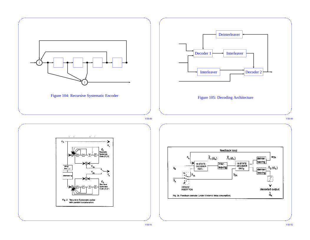
Figure 104: Recursive Systematic Encoder

VIII-89

��

��

Decoder 1

Decoder 2

Interleaver

Deinterleaver

Interleaver

Figure 105: Decoding Architecture

VIII-90

��

��

VIII-91

��

��

VIII-92

��

��

VIII-93