Journal of Financial Economics, forthcoming

An Empirical Examination of the Convexity Bias in the Pricing of Interest

Rate Swaps@

Anurag Gupta*

Marti G. Subrahmanyam**

First Version: November 1997Current Version: September 1999

JEL Classification: G13, G14Keywords: Convexity, Interest Rate Swaps, Interest Rate

FuturesForward Rate Agreements, Term Structure Models

*Department of Banking and Finance, Weatherhead School of Management, Case Western Reserve University, 10900 Euclid Avenue, Cleveland, Ohio 44106-7235. Tel: (216) 368-2938, Fax: (216) 368-4776, e-mail: axg77@po.cwru.edu.**Department of Finance, Leonard N. Stern School of Business, New York University, Management Education Center, 44 West 4th Street, Suite 9-190, New York, NY 10012-1126. Tel: (212) 998-0348, Fax: (212) 995-4233, e-mail: msubrahm@stern.nyu.edu.@We are grateful to David Backus, Gerald Bierwag, Young Ho Eom, Stephen Figlewski, Kenneth Garbade, Pete Kyle, Matthew Richardson, Pedro Santa-Clara, and the referee, Francis Longstaff, for detailed comments on earlier drafts. We also thank seminar participants at New York University, Pennsylvania State University, and the University of Strathclyde, and conference participants at the European Finance Association meetings in Fontainebleau, the Derivatives Securities Conference at Boston University, the Western Finance Association meetings in Santa Monica, and the European Financial Management Association meetings in Lisbon, for comments and suggestions.

Abstract

This paper examines the convexity bias, caused by the non-linearity of payoffs, in the pricing of interest rate swaps off the Eurocurrency futures curve. The evidence from four major currencies – $, £, DM and ¥ - during 1987 to 1996 suggests that swaps were initially being priced off the futures curve (ignoring the convexity adjustment); subsequently, the market swap rates drifted below the rates implied by futures prices. After rejecting alternative explanations, we use alternative term structure models to show that the convexity bias is related to the empirically observed swap-futures differential. We interpret these results as evidence of mispricing of swap contracts during the early years, which was eliminated over time.

2

1. Introduction

Does the market price interest rate swaps correctly? This is a pertinent question for a market that has grown tremendously over the last 10 years, to reach a stage where, according to the International Swaps and Derivatives Association, the notional principal amount outstanding as of December 31, 1998 was about $51 trillion. Since the notional amounts involved are large, a pricing error of even a few basis points in this market quotation translates into large dollar amounts – for example, a six basis-point spread on a $200 million, 10-year swap is worth about $1 million. Despite the size of this market and the consequent importance of accurate pricing, the theoretical and empirical research on the pricing of interest rate swaps is relatively sparse.

The Eurocurrency futures markets and the interest rate swap markets are intimately linked to each other, due to the fact that traders almost invariably hedge their swap positions with Eurocurrency futures (e.g., short swaps can be hedged with short positions in a strip of appropriate Eurocurrency futures contracts). This close relationship has prompted the use of interest rates implied by Eurocurrency futures prices in pricing swaps, which causes an upward bias in implied swap rates, because the forward rates that should be used to price swaps are lower than the rates implied by Eurocurrency futures prices, due to the highly negative correlation between overnight interest rates and futures prices. This bias, known as the convexity bias, arises because of the negative convexity exhibited by (pay fixed) interest rate swaps, while Eurocurrency futures contracts have no convexity since their payoffs are linear in the interest rates. Hence, futures prices should be corrected for convexity before using them for computing swap rates. This paper looks at whether this convexity correction has been incorporated efficiently into interest rate swap pricing over time in the four major international currencies – US Dollar, British Pound Sterling, German Deutschemark, and the Japanese Yen.

Prior research in this area has primarily focused on comparing futures and forward prices and explaining the differences between the two prices. One of the earliest theoretical studies, by Cox, Ingersoll, and Ross (1981), shows that contractual distinctions between futures and forward contracts would create a price divergence even in an efficient market with no transactions costs.1 The argument is based on 1 See also the related papers by Jarrow and Oldfield (1981) and Richard and Sundaresan (1981).

3

the marking-to-market (daily resettlement) feature of futures contracts, which affects the timing of the cash flows between the two counterparties to the contract. On a discounted basis, this difference in payment streams between futures and forward contracts creates a price divergence. Cox, Ingersoll, and Ross use arbitrage arguments to show that the price differences increase with the covariance of the futures price changes with the riskless bond price changes, and if this covariance is positive, then the futures price would be less than the forward price (i.e., the implied forward rate would be lower).

Earlier studies analyze the price differences between forward and futures contracts in the foreign exchange (Cornell and Reinganum, 1981; Muelbroek, 1992) and U.S. Treasury bill markets.2 Although the covariance effects were generally found to be positive and statistically significant in line with the Cox, Ingersoll, and Ross prediction, they are small in magnitude. Perhaps the most important reason for the relatively small size of the effect documented in these studies is the fact that most of the work in these markets relates to relatively short-maturity contracts.

In a recent study, Grinblatt and Jegadeesh (1996) present evidence that the observed spreads between futures and forward Eurodollar yields cannot be explained by the futures contract’s marking-to-market feature.3 They derive closed-form solutions for the yield spread and show that, theoretically, it should be small. They also show that liquidity, taxation, and default risk cannot account for the large spreads observed, and that the spreads are attributable to the mispricing of futures contracts relative to the forward rates. However, they only analyze relatively short-term contracts with maturities up to one year, whereas the spread due to the marking-to-market feature is expected to be more pronounced only in longer-term contracts.

Thus, overall, the empirical research on pricing futures versus forward contracts has examined the data for relatively short-term contracts. Since long-term swap

2 There have been several studies of the Treasury bill market; Rendleman and Carabini (1979), Elton, Gruber, and Rentzler (1984), Park and Chen (1985) and Kolb and Gay (1985) are examples.3 Other explanations for the differences between forward and futures contracts in the Eurodollar market include studies by Kamara (1988) and Sundaresan (1991). Kamara (1988) suggests that differences in liquidity give rise to the futures-forwards price differences. Sundaresan (1991) argues that the “settlement to yield” feature of the Eurodollar futures contract (as opposed to settlement to prices) implies that the forward prices would differ from futures prices, even in the absence of marking-to-market.

4

contracts involving forward commitments of five years and longer are commonplace in the financial markets, it is worth examining how large the differences are for such contracts.

In spite of this literature on the futures-forwards yield differences, there has been no systematic study investigating the impact of these differences in the interest rate swaps market.4 Studies on swap pricing have generally focused on the impact of counterparty default risk on swap rates.5 Koticha (1993) and Mozumdar (1996) examine the impact of the slope of the term structure on the default risk in swaps. Koticha finds that the coefficient of the slope term is negative and significant. Mozumdar (1996) uses a non-linear specification for swap pricing and finds that the default risk parameter is positive and statistically significant in the case of dollar swaps, but not for DM swaps. Sun, Sundaresan and Wang (1993) examine the effect of dealer’s credit reputations on swap quotations and bid-offer spreads.

A recent study by Minton (1997) concludes that swap valuation models based on replicating portfolios of non-callable corporate par bonds or on replicating portfolios of Eurodollar futures contracts perform well, though they are not completely consistent with the implications of differential counterparty default. Minton does not consider the convexity adjustment while pricing swaps off the Eurodollar futures curve. She reports that OTC swap rates do not move one-for-one with equivalent swap rates derived from Eurodollar futures prices, and attributes this lack of equivalence between OTC swaps and the corresponding Eurodollar strips to the absence of counterparty default risk in the futures market.

The objective of this paper is to study the impact of the convexity bias on the pricing of interest rate swaps, and the incorporation of this correction into swaps pricing over time. We will use alternative models of the term structure of interest rates such as those of Vasicek (1977), Cox, Ingersoll, and Ross (1985), Black and Karasinski (1991), Hull and White (1990), and Heath, Jarrow, and Morton (1992), to estimate the convexity adjustment. We also examine whether other explanations such as default risk differences, term structure effects, liquidity differences, or information asymmetries between the swaps and the Eurocurrency futures markets can explain

4 Burghardt and Hoskins (1995) compare swap rates with Eurodollar strips, and report a systematic bias in the prices of interest rate swaps, but do not examine the empirical significance of this bias or potential explanations for it.5 See Cooper and Mello (1991), Litzenberger (1992), Duffie and Huang (1996), Duffie and Singleton (1996) and Baz and Pascutti (1996), for example.

5

the observed pricing differences.

The remainder of the paper is organized as follows. In Section 2, we present a theoretical framework for valuing swaps and relate the convexity of swaps to the differences between futures and forward contracts. Section 3 and the Appendix analyze the convexity correction in swaps and futures using alternative term structure models. Section 4 contains a description of the data sample and a brief overview of the issues involved in constructing the yield curve using futures prices. In Section 5, we present empirical evidence of mispricing of swap rates due to the convexity bias and show that the mispricing cannot be explained by other factors such as counterparty default risk, information asymmetry, or liquidity effects. In Section 6, the alternative term structure models are empirically estimated, and then used to calculate the magnitude of the convexity bias for pricing swaps of varying maturities. We conduct tests to examine whether the theoretically computed convexity corrections are significantly related to the empirically observed spread between OTC swap rates and swap rates computed from Eurocurrency futures prices. Section 7 concludes.

2. The pricing of interest rate swaps

A plain vanilla fixed-for-floating swap is an agreement in which one side agrees to pay a fixed rate of interest in exchange for receiving a variable/floating rate of interest during the tenor (maturity) of the swap. The other counterparty to the swap agrees to pay floating and receive fixed. The two interest rates are applied to the swap’s notional principal amount. The fixed rate, also called the swap rate, is set against a floating reference rate (which is usually LIBOR, the London Inter-Bank Offered Rate). The floating rate is reset several times over the swap’s life – usually every three to six months. Since the interest payments are computed on the same notional principal for both the counterparties, there is no exchange of principal between them at maturity.

Interest rate swaps of all types and maturities are traded in the over-the-counter (OTC) markets. At the initiation date, the market value of the swap is usually set to zero. In the absence of default risk, the arbitrage-free fixed swap rate should equal the yield on a par coupon bond that makes fixed payments on the same dates as the floating leg of the swap. Hence, one method of valuation of a swap on any date after

6

it is initiated is to equate the present value of the floating payments on a reset date to par and net out its present value from the present value of the fixed payments on the valuation date.

An alternative method of valuing a swap contract is to treat it as the sum of a series of forward rate agreements (FRAs).6 This follows because the cash flows of a default-free par swap can be replicated by the cash flows of a portfolio of FRAs maturing at consecutive settlement dates. At each swap payment date, the gain or loss in the currently maturing implicit forward contract is realized. Since FRA rates are not always readily quoted, they can, in principle, be imputed from the prices of Eurocurrency futures contracts.

Although prices of LIBOR forward contracts (FRAs) are available, their liquidity is small, especially for long-dated contracts. Since Eurocurrency futures prices are based on LIBOR rates, they can be used to calculate the relevant forward rates. Many swaps are settled on a semi-annual or annual basis, while Eurocurrency futures contracts are based on 3-month rates, so it is necessary to use two or more futures contracts to hedge each FRA. For example, a short position in a FRA on the six-month LIBOR can be replicated by a portfolio of long positions in two successive Eurocurrency futures contracts. The basic difference between forward and futures contracts is the daily marking-to-market feature in futures contracts, which is examined below.

2.1. Futures-forwards yield differences and swap convexity

Although they are both driven by the same kinds of interest rates, interest rate swaps and Eurocurrency futures contracts differ in one key respect. In a swap contract, cash is exchanged only once for each leg of the swap, but in a Eurocurrency futures contract gains and losses are settled every day. This affects the relative valuation of these two derivative instruments.

To illustrate the contract definitions and payoffs, we use the following notation:

t = valuation date,6 A third method for valuing a swap is by considering a reversal of the swap at the market swap rate. This would yield an annuity equal to the difference between the fixed payments at the original swap rate and the new swap rate, which can be easily valued, since the cash flows are known.

7

T = expiration date of the futures or the forward contract, andT+m = expiration date of the deposit/loan underlying the futures or the forward

contract, where m is the tenor of the underlying interest-rate period.

In the case of Eurocurrency futures, the only source of risk is the change in the futures rate at time t, since all gains/losses are settled right away. On the other hand, swaps are exposed to changes in both the forward rate, and the term rate, i.e., the rate from t to T. The nominal gain on a short swap (conventionally, the short side in a swap receives fixed payments) when the forward rate falls is equal to the nominal loss on the position when the forward rate rises. The present values of the gain and the loss on the swap are not the same, however, because the price at time t of a zero-coupon bond maturing at time T is likely to rise as forward rates fall and vice-versa. Since the discount factor from time t to T behaves asymmetrically with respect to increases and decreases in forward rates, the gain on the short swap is worth more when the forward rates fall because the discount rate used to calculate the present value of the gain also falls. Conversely, the loss on the swap when forward rates rise is worth less because the discount rate for valuing this loss (from time t to T) is higher. The price-yield relationship for the short swap position exhibits positive convexity; i.e., the price increases more when yields falls than the price falls when the yields rise. Eurocurrency futures, on the other hand, exhibit no convexity at all. As a result of this difference in the convexities of the two instruments, a short swap hedged with a short position in Eurocurrency futures benefits from changes in the level of interest rates.

The value of this convexity difference depends on several factors. First, higher volatility of interest rates implies a greater value of the convexity difference. Second, the correlation between changes in forward rates (between T and T+m) and changes in term rates (between t and T) determines whether the value of the convexity difference will be positive or negative. A positive correlation between the two interest rates implies a positive value for this difference, which is usually the case, as forward interest rates and zero-coupon rates tend to be highly correlated. Third, the convexity difference is more pronounced for longer maturity swaps, as the impact of zero-coupon rates on the discounted present value of gains and losses is higher. The difference also depends on the tenor of the underlying interest rate index, say three months or six months, but this effect is small.

The basic reason for this convexity difference between swaps and futures can be

8

traced back to the convexity difference between forwards and futures. In valuing a swap, we need to use forward rates to discount cash flows. Futures rates are sometimes used as proxies for forward rates (as forwards are not actively traded), which is technically incorrect, because there are significant pricing differences between futures and forward interest rates. Effective forward rates need to be imputed from the equivalent futures before they can be used for pricing purposes. The differences in market structures theoretically imply a difference in the yields between futures and forward contracts.7

In general, as shown by Cox, Ingersoll, and Ross (1981), the forward price equals the futures price plus a convexity adjustment term. This additional term reflects the covariance between the T+m maturity zero-coupon bond’s price and the spot rates over the time period [t,T]. When interest rates are deterministic, or when the future spot price is known with certainty, this covariance term is zero, and hence forward and futures prices are identical.

The difference in convexity between forward and futures contracts can be theoretically decomposed into two components - the term effect, due to the maturity of the contract; and the tenor effect, due to the fact that there is a time lag between the time when the interest rate is observed and the time when the corresponding payoff occurs. Suppose f(t,T,T+m) refers to the price of a forward contract at time t, expiring at time T, on an interest rate of tenor m, i.e., between time T and time T+m. The notation is similar for the price of a futures contract, (F(t,T,T+m)). For a forward contract, (f(t,T,T+m)), and a futures contract, (F(t,T,T+m)), the term effect corresponds to the convexity differential due to the stochastic discount factor between time t and time T, while the tenor effect refers to the convexity introduced by the stochastic discount factor, between time T and time T+m (corresponding to the tenor of the underlying interest rate). As the maturity of the contract increases, the term effect accounts for a larger proportion of the total convexity differential.

7 Futures and forward contracts are both agreements between two parties to trade a specific good or an asset at a future date for a pre-determined price, but they are settled quite differently. Futures contracts are standardized contracts, traded on organized exchanges. The futures exchange virtually eliminates default risk by assuming the opposite side of each trade, guaranteeing payment. Positions are marked-to-market every day to reduce default, as gains/losses are settled on a daily basis. On the other hand, forward contracts, traded mostly in the OTC markets, are exposed to default risk. They are not standardized, with all payments made at the maturity of the contract. Moreover, forward positions can be synthetically replicated by taking positions in the cash market. For example, a trader can create a forward position in a three-month time deposit starting three months in the future by going long a LIBOR deposit with a six-month maturity and going short the LIBOR deposit with a three-month maturity.

9

The tenor effect shows less variability; it is affected only by the level, volatility, and tenor of the interest rates, and not by the maturity of the contracts. In this paper, hereafter, the convexity differential refers to the total convexity bias, which is a combination of the term and tenor effects.8

Empirically, it has been shown that a significant yield difference exists between these two contracts, with forward yields being lower than the corresponding futures yields to which they are tied, since the correlation between the overnight interest rate and the price of the futures contract is negative. Since forward rates should be used to value swaps, the use of futures rates without correcting for convexity would impart an upward bias to swap yields. In that case, the spread between market swap yields and the implied swap yields (computed directly off the Eurocurrency futures curve without correcting for convexity) would fluctuate randomly around zero. If the swap market recognizes this mispricing and corrects futures rates for convexity fully, this spread should be negative (as the convexity correction would lower the swap yield, thereby making the market yield lower than the raw, unadjusted implied swap yield). It follows, therefore, that a zero spread between market and unadjusted swap yields is an indication of market inefficiency. 3. Theoretical derivation of the convexity adjustment

The differences between futures and forward rates, which lead to the convexity bias in interest rate swaps, are potentially attributable to the marking-to-market feature of futures contracts. This section characterizes these differences, using five different term structure models, to examine the impact of different assumptions about the underlying interest rates on the convexity adjustment. Closed-form solutions can be derived for the Eurocurrency futures-forward rate differences using the Vasicek (1977) and Cox, Ingersoll, and Ross (1985) models, while the trinomial tree approach of Hull and White (1993, 1994) can be used to numerically estimate the convexity bias for the no-arbitrage models of Hull and White (1990) and Black and Karasinski (1991). All these models can be related to the general formulation of Heath, Jarrow, and Morton (1992). In particular, a two-factor specification with a constant volatility function can be implemented using a non-recombining tree for the evolution of the forward rate curve to estimate the impact of a two-factor model

8 We considered separating the two convexity effects in the empirical work that follows. However, since the variability of the tenor effect is likely to be very small, virtually all of the variation would come from the term effect. Hence, we decided to focus on the total convexity effect in our empirical work.

10

on the convexity bias.

In order to price convexity, a model of interest rates is needed to provide an unambiguous description of the evolution of rates. The model needs to be rich enough to allow for a wide variety of future yield environments while at the same time constraining the yield movements within reasonable bounds. There is also a trade-off between analytic tractability and numerical accuracy and consistency. The models of Vasicek and Cox, Ingersoll, and Ross allow for analytic solutions, but they do not fit the current yield curve exactly, thereby introducing a pricing error in the underlying zero-coupon bonds themselves. The no-arbitrage models of Hull and White, Black and Karasinski, and Heath, Jarrow, and Morton are numerically consistent with the current prices of zero-coupon bonds, but they are computationally intensive. The Black and Karasinski model is also analytically intractable because of the assumption of lognormal interest rates. We briefly describe the expressions for the convexity adjustments in the context of these models in the Appendix.

Multi-factor models are not likely to make much of a difference to the estimates of the convexity adjustments in certain interest rate environments. Examples would be cases in which the correlations across points on the yield curve are high or the variances of the additional factors, after orthogonalization, are relatively small. The use of multi-factor models may be important for pricing instruments when these correlations are important (e.g., swaptions, mortgage-backed securities, or bond options). To examine whether the size of the convexity adjustment is affected by multiple factors, we estimate a two-factor Heath, Jarrow, and Morton model.4. Data

The data for this study consist of daily Eurocurrency futures and interest rate swap rates over 10 years (1987-1996) for the four major currencies – US Dollar (USD), British Pound Sterling (GBP), German Deutschemark (DEM), and Japanese Yen (JPY). All the rates and prices are closing, midmarket quotes (average of bid and ask quotes). The swap rates and Eurocurrency futures prices were extracted from DataStream. To check the quality of the data, we also obtained Eurocurrency futures prices from the Futures Industry Association. We find no significant differences or outliers in the two data sets. The swap rates were randomly checked against historical quotes maintained by Bloomberg Financial Markets, and again there were

11

no significant differences between the two sources.9 The fixed-for-floating interest rate swaps studied consist of maturities of two, three, four and five years for USD, and maturities of two years for GBP, DEM and JPY. We could not study swaps with a maturity longer than two years for GBP, DEM and JPY due to the poor liquidity of the respective Eurocurrency futures contracts for longer maturities. Daily spot one- to three-month LIBORs were also taken from DataStream.

We need to make a few adjustments to make the Eurocurrency futures data comparable with the swap data. First, since Eurocurrency contracts are based on quarterly maturities, it is necessary to combine two or more contracts to obtain longer maturity rates. For instance, the six-month zero-coupon rate on a futures expiration date is obtained by combining the rates implied by two successive Eurocurrency contracts. Second, it is necessary to use the spot LIBOR rates and interpolate between futures rates to obtain the zero-coupon rates on dates other than the futures maturity dates. Third, the swap day-count conventions vary across currencies, and we must take this variation into account in determining the payment amounts and dates.10 Once we obtain these rates, the swap can be priced by computing the yield on a par coupon bond with the same maturity and coupon dates as the swap.11

In this paper, we estimate a single yield curve using data from the cash market out to the first futures expiration date (zero- to three-month maturity, depending on the date), and then data from the futures market out to ten years. The high density of cash market data for short-term maturities helps define the shape of the Eurocurrency yield curve at the extreme front end. We use the cubic spline

9 Sun, Sundaresan, and Wang (1993) have documented that swap rates obtained from DataStream and Data Resources, Inc. (DRI) are not economically different from each other.10 For example, in the USD swap market, the day count is 30/360 with semi-annual payments; in the DEM market, it is 30/360 with annual payments, while in the JPY market, the day-count convention is Actual/365 with semi-annual payments. The underlying floating rate also varies across currencies; for instance, in the case of the USD swap market, it was the six-month LIBOR.11 The discount functions to value swaps should ideally be obtained using the swap yield curve, but insufficient data from liquid contracts prevent that from being done. The only publicly available market data are for swap coupons on new, plain-vanilla swaps with maturities of two, three, four, five, seven, and ten years. Market values of swaps with odd maturities, non-standard coupons, or exotic features are not publicly available. Hence, the prices of swap contracts have to be imputed from the prices of some other actively traded financial instruments for which the prices are competitively determined and publicly available. For this purpose, it is common practice to use three-month Eurocurrency futures prices to derive the LIBOR term structure, the market for which is deep for maturities going out to at least three to five years. See Garbade (1990) for further details.

12

interpolation method to define the complete shape of the yield curve.12

5. Empirical evidence

We have two sets of data on the swap markets. The first is the series from the swap market quotations, and the second the series implied by the zero-coupon rates calculated from the Eurocurrency quotations. We refer to the difference between these two rates on a given date for a particular maturity and currency as the swap-futures differential.

Table 1 and Figure 1a present the descriptive statistics for market swap rates and the swap-futures differential for US dollar swaps. In general, the implied swap rates are found to be lower than the market quotes. For example, the average implied swap rate for five-year USD swaps is lower than the average market rates by about 9.31 bp. The difference is seen more clearly when the data are segmented into three time periods – 1987-90, 1991-93, and 1994-96. This segmentation is primarily based on the interest rate environment during these years, shown in Figure 1. During the first subsegment, i.e., 1987-90, interest rates are relatively high, but stable. In this period, the slope of the swap term structure is relatively low, with a remarkably low volatility in swap rates (less than 0.7% for all swap maturities). On the other hand, the volatility in the swap-futures differential measured by its standard deviation is the highest in this subperiod for two-year swaps (4 bp), and is relatively high for three-year swaps (2.8 bp). The very low value of the differential in this period (on average less than 1 bp) suggests, prima facie, the pricing of swaps right on the Eurodollar futures curve (thus implying mispricing due to the convexity bias).

The second subperiod (1991-93) corresponds to an era of declining interest rates. The swap term structure is steep during this period (126 bp, on average, between a two-year and a five-year swap), and so is the volatility of swap rates (about 1.2-1.3%). The value of the swap-futures differential is the highest for this subperiod (averaging 8-10 basis points for swaps of various maturities), indicating a trend towards recognition and incorporation of the convexity correction in the pricing of swaps (with market quotes being lower than the corresponding rates implied from Eurodollar futures prices). The volatility of the swap-futures differential is also lower

12 Cubic spline interpolation has been extensively used in term-structure modeling, starting with McCulloch (1971).

13

during this period. In the third subperiod (1994-96), there is again an increase in interest rates, along with a flattening of the swap term structure, though the volatility of swap rates is relatively high (about 0.8%, primarily due to the high volatility of interest rates in this period). The swap-futures differential is significantly negative (at the 1% significance level) for this subperiod for all maturities (the average differential varying between 6 bp for two-year swaps and 10 bp for ten-year swaps).

From Table 1, it can be seen that swap rates derived from Eurodollar futures prices are greater than market swap rates for all maturities as well as in every subperiod. The differential between these two rates is insignificantly different from zero for the first subperiod (1987-90), while it is significantly negative for the second subperiod (1991-93). During the third subperiod (1994-96), the swap-futures differential is negative and significant at the 1% level for all swap maturities. The mean differential is increasing in swap maturity, which is consistent with the hypothesis that longer-dated swaps exhibit greater convexity. The evidence is also consistent with the hypothesis of swaps being priced right off the Eurodollar futures curve during the earlier years, and then being adjusted for convexity in later years. The absolute amount of the convexity adjustment, that is a function of term-structure parameters such as volatility, varies over time. The volatility of the swap-futures differential is uniformly decreasing in the swap maturity, implying higher significance levels for longer dated swaps. This is also consistent with the fact that convexity increases with maturity.

Figure 2 presents the time-series plots of the swap-futures differential for USD swaps of two-year maturity. The plots for three-, four- and five-year maturity are similar. This figure clearly indicates pricing of swaps right on the Eurodollar futures curve until 1991, and then a gradual incorporation of the convexity adjustment. This is indicated by the negative drift in the swap-futures differential after 1991, followed by stabilization of the market swap rate below the rate implied by Eurodollar futures.

Table 2 and Figure 1b present similar descriptive statistics for swaps in the pound sterling market. The swap rates and swap-futures differential exhibit a behavior similar to the US dollar market. A lower volatility in swap rates is accompanied by a higher volatility in the differential. The differential in the first two subperiods is either positive or insignificantly different from zero, while it is significantly negative during 1994-96, indicating incorporation of the convexity adjustment during this

14

period. Thus, the swap-futures differential suggests mispricing upto 1992, and then incorporation of the convexity adjustment (by way of a negative drift in the differential).

As shown in Table 2 and Figure 1b, we obtain similar results for the DEM and JPY markets.13 There is strong evidence of mispricing of swaps upto 1994, after which there is evidence of incorporation of convexity adjustment in swaps pricing.

In all these markets, the swap-futures differential is too large to be explained by difference in the two markets in terms of bid-ask spreads (which are typically less than 3-4 basis points in the swaps market) or measurement error due to asynchronicity in the exact timings of these quotes (both swaps and futures prices are closing-day quotes). Moreover, there is no reason to expect these two factors to bias the differential in one direction. Before making an adjustment for convexity, we will first attempt to explore alternative explanations for the differential.

Several alternative explanations have been proposed for the differential pricing of swaps in relation to Eurocurrency futures contracts:14

1. Counterparty default riskSwaps, being traded in the over-the-counter market, are exposed to counterparty default risk, while Eurocurrency futures, which are exchange-traded, are virtually free of default risk because of the implicit guarantee of the contracts provided by the clearinghouse and backup margins/collateral.

2. Information asymmetriesEurocurrency futures are contracts traded on organized exchanges. Due to very high trading volumes and open interest, these markets are closely scrutinized by traders and investors. Hence, these markets can be assumed to be reasonably efficient, in terms of current information being reflected in prices. The swap market, on the other hand, is an OTC market with lower volumes (especially for longer-dated swaps) and less standardization. Hence, the swap markets may not be as informationally efficient as the Eurocurrency futures markets.

13 The analysis for DEM and JPY swaps is from 1991 onwards, due to the lack of Eurocurrency contracts of two-year maturity prior to 1991, which prevents swap replication using Eurocurrency futures.14 A fourth possibility, which is an aspect of default risk, was also examined and found to be unimportant. This relates to the effect of the slope of the term structure on the default risk. In the presence of stochastic interest rates, proxies for changes in the yield curve should be empirical determinants of swap rates. Hence, it was examined whether changes in term structure parameters affect swaps differently from futures.

15

3. LiquidityThe Eurocurrency futures market is a very active market characterized by very high trading volumes. The interest rate swap market is very liquid today, but was not very liquid during the late 1980s and early 1990s. Illiquidity in swaps, therefore, could have increased the market swap rates, so that it is possible for the liquidity premium to raise the swap rate to (or above) the level of the rate implied from Eurocurrency futures prices, even if they were convexity-corrected.

5.1. Counterparty default risk

If there is a significantly higher default risk in swaps, then the pricing of swaps should incorporate it, and the market swap rate should be correspondingly higher. Yet, as Litzenberger (1992) first observed, the default risk of interest rate swaps is significantly mitigated by several factors:

1. Only net interest payments, and no principal payments, are exchanged.2. Many swaps have netting provisions, which stipulate that in the event of default

the counterparties settle all contracted liabilities.3. A firm’s probability of defaulting on a swap is much lower than on a bond, as the

former probability reflects the joint probability of the firm being financially distressed and the swap having a negative value to the firm.

4. Swaps with counterparties whose credit quality is lower are often collateralized, so that the potential loss in the event of default is reduced.

The default risk of swap contracts nevertheless is still marginally higher than the default risk of futures contracts, since the latter are marked-to-market each trading day (and are, therefore, subject to the guarantee of the clearing house and the posting of margins). To examine whether this differential default risk can explain some part of the variation in the swap-futures differential, we present the estimates of five regression models:

I. Swap Difft = a + b(TED Spread)t + t , (1a)

II. Swap Difft = a + b( TED Spread)t +t , (1b)III. Swap Difft = a + b( AAA-Govt)t +t , (1c)IV. Swap Difft = a + b( BBB-AAA)t +t , (1d)

V. Swap Difft = a + b(TED Spread)t + c( AAA-Govt)t

+ d( BBB-AAA)t + t . (1e)

16

In models I and II, the TED spread (Treasury-Eurodollar spread measured as the difference between three-month Eurodollar time deposit rates and three-month treasury rates) is used as an explanatory variable for the variation in the swap-futures differential. Treasury bills are free from default risk, but Eurodollar deposits are based on the LIBORs. When the banking industry as a whole does poorly, LIBORs increase significantly relative to Treasury bill yields, thereby increasing Eurodollar deposit rates. Thus, the TED spread tends to widen in times of financial crisis and tighten in periods of stability, and it is widely regarded as a measure of aggregate default risk of banks at the short end of the term structure.

We examine next the impact measures of default risk at the long end of the term structure. In regression model III, the AAA-Govt spread (defined as the spread between monthly averages of the AAA bond yields and the long-term government bond yields reported by Standard & Poor’s) is used as the explanatory variable, while in regression model IV, the BBB-AAA spread (defined as the spread between monthly averages of the BBB and the AAA bond yields reported by Standard & Poor’s) is the explanatory variable. Both of these variables are aggregate measures of corporate default risk at the long end of the term structure. The AAA-Govt spread is a measure of “one-sided” corporate default risk because government bonds (in the home currency) are default-free. The BBB-AAA spread is used as a measure of “two-sided” default risk in the corporate sector. These spreads tend to increase when the corporate sector’s default risk goes up. Hence, these spreads are presumed to capture the effects of the corporate default risk. Model V is estimated as a multivariate regression with first differences of the three variables (TED Spread, AAA-Govt, and BBB-AAA) used to explain the variation in the swap-futures differential. This multivariate test controls for the interaction between the independent variables to examine their combined effect, if any, on the swap-futures differential.

In Table 3, Panel A, the significantly positive slope coefficients, b, are consistent with the default risk hypothesis : a widening TED spread would imply greater risk of default, thereby implying higher values for the swap-futures differential, as defined. The time series for the swap-futures differential and the TED spread are then tested for nonstationarity. The null hypothesis of non-stationarity fails to be rejected for the TED spread series and for the swap-futures differential time series over all maturities. Hence, because both of these time series are nearly integrated over

17

time, the second regression model is estimated using first differences. It can be seen from Table 3, Panel B that, although significant, the absolute values of the slope coefficients are less than 10% (for regression model II), which implies that a 10-basis-point increase in TED spread corresponds to a less than 1-basis-point increase in the swap-futures differential. More important, the adjusted R2 values are less than 5%, implying that the regression model explains only a very small part of the day-to-day variation in the swap-futures differential. Therefore, while the regression models are statistically significant, they are of low economic significance.

Similarly, the results of regression models III and IV are reported in Table 3, Panels C and D respectively. Due to non-stationarity of the time-series, these two models are also estimated using first differences. The results for model III are insignificant for all swap maturities, indicating that univariate corporate default risk does not explain any variation in the swap-futures differential. The results for model IV are statistically significant (except for swaps of three-year maturity), but the slope coefficients are less than 5%, and the adjusted R2 values are around 4%. The results for the multivariate test (presented in Table 3, Panel E) suggest some significance for the coefficient of the BBB-AAA spread, but the adjusted R2 values are even lower than those for the univariate test. Hence corporate default-risk proxies (individually, as well as in combination with an aggregate economy-wide default-risk proxy) also fail to explain the variation in the swap-futures differential. We can conclude, therefore, that default risk does not explain the differential between market and futures-implied swap rates.

5.2. Information asymmetries

We next consider whether timing differences in information flows across the two markets explain the differential between market swap rates and swap rates implied by Eurocurrency futures prices. If changes in one rate can predict future changes in the other rate, then the information relevant for future interest rates is not being incorporated into the swap and futures markets simultaneously.

We examine whether changes in the swap rate implied from Eurocurrency futures prices lead the changes in market swap rates. If this were true, it would imply that Eurocurrency futures markets are informationally more efficient than swap markets. Table 4 presents estimates of the following univariate regression:

18

+1, Mkt Swap = a + b ,- Euro Swap + , = 0,1,2,5,10,20 (2)

In this model, daily changes in the market swap rate are regressed on lagged daily changes in implied swap rate. To take care of all possible lagged effects, the regressions are done for lags of one, two, five, ten and twenty days. Since these days are defined as actual trading days, a lag of five days corresponds to a week, while a lag of twenty days corresponds to approximately one month. The results in Table 4 for the US dollar markets show that almost all of the information is simultaneously incorporated into the swap and the futures rates. Lag 1 and lag 2 regressions have significant coefficients for all swap maturities, but with much lower slope values (20% and 10% respectively) and very low R2 values (4% and 2% respectively). The predictability in futures rates is therefore economically insignificant. Beyond lag 2, many of the coefficients are not significant, with R2

values below 1%. Similar inferences can be drawn for the British pound sterling, German Deutschemark, and Japanese yen markets from the results presented in Table 4.

We also test the predictability of market swap rates from implied swap rates using lagged daily changes (up to a lag of five days) in the implied swap rates in a multivariate regression. We find that the contemporaneous change in the implied swap rate explains nearly all of the variation in the market swap rate, with a coefficient close to one. The lag 1 change in the implied swap rate has a much lower coefficient of 8% - 9% (depending on the maturity of the swap), though it is statistically significant, implying some predictive power in the previous day’s change in the implied swap rate. Beyond lag 1, however, virtually all of the slope coefficients are insignificantly different from zero. Similar multivariate regression results for the other three markets (pound sterling, Deutschemark, and yen) further reinforce the conclusion that there are virtually no delays in the flow of information from the futures market to the swap market.

We further test whether there is a significant delay in the flow of information from the swap market to the futures market. In that case, lagged changes in the market swap rate should predict changes in the swap rate implied from futures prices. We regress the changes in the implied swap rate on the contemporaneous and lagged changes in the market swap rates. Again, in all four markets, the coefficient for the

19

contemporaneous changes in the market swap rate is highly significant, while most of the other slope coefficients (for lagged changes in the market swap rate) are not significantly different from zero. There is, therefore, no significant evidence that market swap rates are able to predict implied swap rates.

The results presented thus far indicate that there is virtually no information asymmetry between the swap and the Eurocurrency futures markets, for all the four currencies analyzed. The swap-futures differential observed in these markets cannot be attributed to informational reasons.

5.3. Liquidity

If liquidity were the cause for the observed swap-futures differential, then a suitable proxy reflecting the liquidity in the interest rate swap market should explain the differential. The gradual disappearance of this liquidity premium over time would then cause the swap-futures differential to drift below zero.

To test this hypothesis, we estimate the following two regression models:

I. Swap Difft = a + b(Bid-Ask Spread)t + t ,(3a)

II. Swap Difft = a + b( Bid-Ask Spread)t +t ,(3b)

where the bid-ask spread in swap rates is used as a proxy for liquidity in the swap market (a higher bid-ask spread reflects lower liquidity and vice-versa).15 Since the time series for the swap-futures differential and for the bid-ask spreads are nearly integrated over time, the second regression model is estimated using first differences. Table 5 presents the results of these regressions for USD swaps of two-, three-, four- and five-year maturity. It can be seen that the changes in bid-ask do not explain any variation in the swap-futures differential, when the regression model is estimated using first differences to correct for serial correlation. The increasing liquidity of the swap market cannot be the cause for the observed behavior of the

15 Bid-ask spreads were as high as 12-15 basis points in the swap market in the 1980s, while they have now decreased to 2-3 basis points.

20

swap-futures differential.

The empirical analysis in this section indicates that several alternative explanations for the swap-futures differential – credit risk, information asymmetry and liquidity effects – do not explain much of the variation in the swap-futures differential, although some of the factors are statistically significant. In the following section, we investigate the impact of the convexity adjustment on the differential.

6. Empirical estimation of the convexity adjustment

6.1. The Vasicek and Cox, Ingersoll, and Ross models

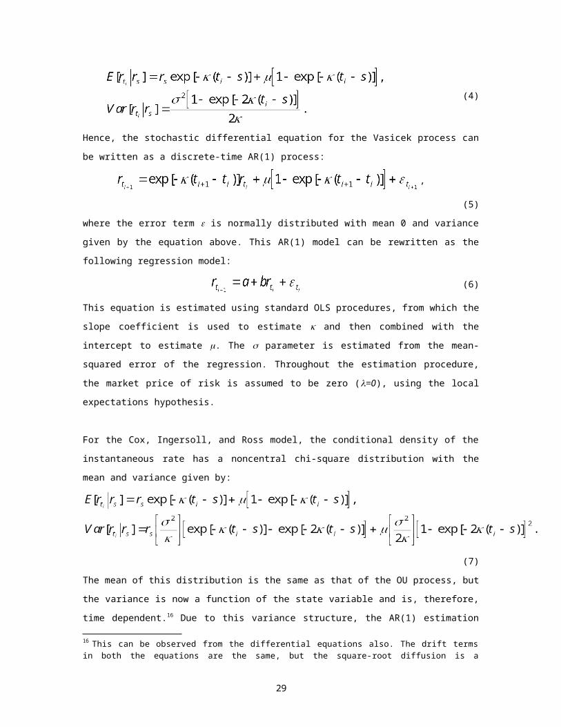
For the Vasicek (OU) process [Eq. (A.1) with =0], the conditional density of the instantaneous interest rate at any future date ti, given today’s level of instantaneous rate (rs), is a normal distribution with mean and variance as follows:

(4)

Hence, the stochastic differential equation for the Vasicek process can be written as a discrete-time AR(1) process:

, (5)

where the error term is normally distributed with mean 0 and variance given by the equation above. This AR(1) model can be rewritten as the following regression model:

(6)This equation is estimated using standard OLS procedures, from which the slope coefficient is used to estimate and then combined with the intercept to estimate . The parameter is estimated from the mean-squared error of the regression. Throughout the estimation procedure, the market price of risk is assumed to be zero (=0), using the local expectations hypothesis.

21

For the Cox, Ingersoll, and Ross model, the conditional density of the instantaneous rate has a noncentral chi-square distribution with the mean and variance given by:

(7)The mean of this distribution is the same as that of the OU process, but the variance is now a function of the state variable and is, therefore, time dependent. 16 Due to this variance structure, the AR(1) estimation procedure has to be modified. The regression model is still the same as in Eq. (6), but the error term is no longer identically and independently distributed. Since it is a function of the state variable, ordinary least squares (OLS) does not apply. It can be viewed as a regression model with heteroskedasticity, which can be estimated using weighted least squares. In the first step, Eq. (6) is estimated using OLS, from which estimates of and are obtained. Since the conditional variance of the errors from this regression must be as specified by Eq. (7), a second regression is estimated using squared errors as follows:

. (8)The intercept as well as the slope can be used to obtain estimates of the parameter. As done in previous research (see, for example, Chen and Yang (1995)), we choose the alternative that generates estimates more consistent with those from previous studies. As before, the market price of risk is assumed to be zero during this estimation.

Weekly observations of the three-month LIBOR rate are used over the period 1975-1996 to estimate the parameters for USD, GBP and DEM. For JPY, the data used are for the three-month LIBORs from 1978 to 1996. The parameter estimates are reported in Table 6a for the Vasicek and the Cox, Ingersoll, and Ross models. The estimates for USD are very close to those reported by other studies. For the other currencies, no such benchmarks are available, but the parameter values are within reasonable bounds.

6.2. The Hull and White and Black and Karasinski models

16 This can be observed from the differential equations also. The drift terms in both the equations are the same, but the square-root diffusion is a function of the state variable, while the OU diffusion term is constant.

22

The empirical estimation of the Hull and White and Black and Karasinski models is carried out by constructing a trinomial tree for interest rates.17 LIBOR cash rates up to one-year maturity and swap rates upto ten-year maturity are used to construct the LIBOR zero curve (up to ten-year maturity) by a bootstrapping procedure. This LIBOR zero curve is used to calibrate the interest rate tree to fit the initial term structure exactly. We choose the volatility parameter and the mean-reversion parameter a (defined in Eq. (A.13)) so as to provide a “best-fit” to the market prices of interest rate caps. The minimization of squared error is accomplished using a non-linear least squares estimation technique.

6.3. The Heath, Jarrow, and Morton model

The two-factor Heath, Jarrow, and Morton model is implemented in discrete-time using trinomial non-recombining trees. The drift term in the forward rate process is re-estimated in discrete time using no-arbitrage conditions adapted from Jarrow (1996). A constant volatility function is assumed, so the implied spot rate distribution is Gaussian. To ease the burden on computer memory and improve computation speed, we implement the framework using a recursive algorithm proposed by Das (1998). This algorithm eliminates the need to store the entire forward rate tree in the memory by following each sample path to its conclusion in a recursive manner. This frees up memory, potentially allowing an unlimited number of time steps to be used, within the constraints of computing power.

6.4. Convexity bias estimation results

Using these five models, the convexity differential between futures and forwards is presented in Figure 3. The resultant impact of this convexity differential on the bias in swap pricing is presented in Table 6b. The magnitude of the mean spread after 1993 roughly corresponds to the magnitude of the convexity adjustment for swaps of respective maturities, which further reinforces the evidence that the observed drift in the swap-futures differential is due to incorporation of convexity adjustment in swap rates. From Figure 3, it is evident that different assumptions on the underlying interest rate process have a significant impact on the behavior of the convexity adjustment as a function of maturity. The convexity curves are roughly similar for the Hull and White and Black and Karasinski models, in magnitude as well

17 Details of the tree construction methodology can be obtained from Hull and White (1994).

23

as curvature. The Vasicek model estimates are very close to the Hull and White estimates up to three-year maturity contracts, but are significantly lower for longer-dated contracts. A closer look at the parameter estimates for these models provides a possible explanation for this behavior. The estimate of mean-reversion for the Vasicek (and Cox, Ingersoll, and Ross) model (0.2731) is much higher than that for the Hull and White (0.08) or the Black and Karasinski (0.06) models.18 A very high mean-reversion would tend to decrease long rate volatility very significantly, which would lead to a much lower impact of maturity on convexity adjustment. The estimates of the Cox, Ingersoll, and Ross model are also distorted due to this bias.

The results using any of the models suggest that the convexity adjustment can be very large for long-dated contracts. For a ten-year futures contract, our calculations suggest that this adjustment can be on the order of 80-100 basis points, which translates into a convexity adjustment of about 35-40 basis points for a ten-year swap (which “averages out” the adjustment for the cash flows of various maturities up to ten years). Even a conservative estimate of the bias for a five-year USD swap is about 12-16 basis points, which is significantly higher than the bid-ask spread of 3-4 basis points that is observed in the swap market. More significantly, the bias is comparable to the observed swap-futures differential and is in the right direction (i.e., market swap rates are lower than implied rates during the latter years of the study). This supports the hypothesis that the mispricing observed in swap rates during the earlier years of the study (1987-1990) was due to the convexity bias, and that this mispricing has been gradually corrected over time.

6.5. The relationship between the convexity adjustment and market swap rates

As a final check on the robustness of the conclusion that the observed spread between market and futures-implied swap rates is primarily a result of the convexity adjustment, we estimate the following regression model:

18 The Hull and White and Black and Karasinski models have time-varying means, which implies that interest rates are modeled as reverting to a time-varying “target,” instead of a constant one. This reduces the dependence on the reversion speed, leading to lower, and possibly more realistic, estimates of the reversion parameter for these models as compared to those for Vasicek or Cox, Ingersoll, and Ross models. This is also a manifestation of the inability of the single-factor Vasicek or Cox, Ingersoll, and Ross models to satisfactorily describe the curvature of the entire yield curve.

24

Swap Difft = (a0+a1Dt) + (b0+b1Dt)( CA)t +t . (9)

The convexity adjustment (CA) is calculated using the Hull and White model. Dt is a dummy variable that takes the value 0 during the time period 1987-91, and 1 during 1992-96. The dummy variable is used to separate the two distinct pricing regimes – the first one (1987-91) when there is apparent mispricing as convexity adjustments are ignored, and the second one (1992-96) when this mispricing appears to have been corrected. Given that the Hull and White model properly adjusts for convexity, during the second subperiod, a 1-bp change in convexity correction should be reflected in an equivalent 1-bp change in the observed swap-futures differential. By the same token, however, there should not be any significant relationship between convexity changes and the observed differential in the first subperiod. Hence, the null hypothesis is that b1=1 and b0=0. If changes in the convexity are the only factors that affect the changes in the swap-futures differential, the constant terms in Eq. (9) (a0 and a1) should be insignificantly different from zero. Nonzero constant terms that are statistically significant would indicate the presence of other factors that affect the observed swap-futures differential.

Table 8 presents the results of this regression. In Panel A, the model is estimated directly, using OLS. The estimates of the constant terms are significantly different from zero. Hence, this is indirect evidence that the convexity adjustment was not made in the first subperiod. Estimates of a0 and a1 have opposite signs, and the combination of these two results in a constant term close to zero, indicating that, for the second subperiod, the convexity adjustment is fully reflected in the differential.19

The slope coefficient b0 is significantly different from zero. The estimates of b1 are close to 1 only for swaps of two-year maturity. For swaps of three-, four- and five-year maturity, the slope coefficient b1 is significantly less than 1 (between 0.29 and 0.44), while it should be insignificantly different from 1 as per the null hypothesis. This slope coefficient appears to be attenuated towards zero due to measurement error as well as missing variable bias. Hence, we estimate the same regression model in Panel B using the instrumental variables technique to correct for these biases. The instruments used for this estimation are term-structure parameters that are correlated with the convexity adjustments, but uncorrelated with the errors of the original regression model. Using the volatility of interest rates (contemporaneous, lagged by one day, and lagged by two days), the level of

19 In general, one cannot interpret the signs of the coefficients in an unambiguous manner, given the errors-in-variables problem.

25

interest rates, and the slope of the term structure as instruments, the two-stage least squares method is used to estimate the parameters of the model (it can be shown that this IV estimator is unbiased and consistent). The results in Panel B show that the IV estimation technique corrects for the biases to a large extent. The estimates of the constant terms (a0 and a1) are insignificantly different from zero for all swap maturities. The slope coefficient b0 is also insignificantly different from zero (except for two-year maturity swaps). More important, the estimates of the slope coefficient b1 are higher and closer to 1.20 The results in Panel B clearly show that changes in the convexity bias influenced the changes in the swap-futures differential nearly one-for-one during the second subperiod (1992-96), while they had an insignificant impact on the differential during the first subperiod (1987-91).

The results indicate that the swap-futures differential observed during the second subperiod is an outcome of the incorporation of convexity adjustments in swap pricing. The broad conclusion of this regression is that the convexity adjustment appears to have been ignored in the earlier period, while in the latter period the adjustment seems to have been made in market swap rates.

7. Conclusion

This paper examines the incorporation of the convexity bias in the pricing of interest rate swaps from 1987 to 1996, for four major swaps markets – USD, GBP, DEM, and JPY. Empirical evidence suggests that swaps were being priced using raw futures prices, unadjusted for convexity, during the early part of the sample period. During the latter part of the study, market swap rates drift below the swap rates implied by Eurocurrency futures prices. We find the spread between market and futures-implied swap rates to be comparable in magnitude to the theoretical value of the convexity bias estimated using the Vasicek, Cox, Ingersoll, and Ross, Hull and White, Black and Karasinski, and Heath, Jarrow, and Morton term-structure models. We evaluate alternative hypotheses for this observed swap-futures differential (and the changes in this differential over time) using default risk differences, informational 20 The estimate of b1 is still significantly less than 1 for swaps of four- and five-year maturity. This test, however, is a joint test of the convexity estimation model (in this case Hull and White) being correct and the convexity being the only parameter influencing the swap-futures differential. Further, If convexity is generated by a multi-factor term-structure model in the real world, this slope coefficient would be different from one even when convexity is the only parameter influencing the swap-futures differential.

26

asymmetries, and liquidity differences between the swap and the futures markets, but none of these factors offers a satisfactory explanation for this differential. We conclude, therefore, that this is evidence of mispricing of swap rates during the earlier part of the study, with a gradual elimination of this mispricing by incorporation of the convexity correction in swap pricing over time.

Our findings suggest that during the late 1980s and the early 1990s, there was a systematic advantage to hedging a short swap position with short Eurocurrency futures contracts. The reason for this arbitrage was the mispricing of swap rates due to ignoring the convexity correction in the swap curve construction techniques. The arbitrage may have been limited due to market frictions as well as internal or external constraints on bank participation in futures markets. The persistence of significant mispricing for several years goes against the conventional wisdom that any pricing discrepancy between two markets would be quickly arbitraged away.

In future work, we plan to investigate further the linkages, if any, between the convexity bias and the liquidity and credit risk factors.

27

Appendix

A.1. Derivation of convexity adjustment using the Vasicek/Cox, Ingersoll, and Ross models

The Vasicek and the Cox, Ingersoll, and Ross models have the following general form:

dr = (-r)dt + rdz, (A.1)wheredr = change in the instantaneous short rate, = speed of adjustment (mean-reversion), = long run mean of the short rate, = instantaneous short-rate volatility parameter, anddz = standard Wiener process increment.

In the context of this study, the state variable r can be interpreted as the instantaneous (LIBOR) interest rate. The exponent contributes to the determination of the distributional properties of the short rate; =0 implies normally distributed rates (Vasicek), while =1/2 gives the Cox, Ingersoll, and Ross model (the conditional distribution of the short rate is noncentral chi-square). =1 yields lognormal interest rates. The choice of is dictated by a compromise between analytic tractability (=0 and =1/2) and reasonableness of the resulting distribution. The Vasicek specification permits interest rates to become negative.

A.1.1. The Vasicek model

Under the Vasicek model (=0), the short rate follows the Ornstein-Uhlenbeck process and the date s price of a pure discount bond with unit face value maturing at date t is given by

, (A.2)where the functions Av(x) and Bv(x) are defined as

(A.3)

and is the market price of risk per unit of .

Given this solution, the forward rate f(ti, ti+1) at date s can be computed as follows:

. (A.4)

The futures rate F can be shown to satisfy the following partial differential equation [see Grinblatt and Jegadeesh (1996), for example]:

(A.5)subject to the boundary condition that at maturity the futures rate must equal the LIBOR at that date;

. (A.6)Under the Vasicek model, the futures rate F(ti,ti+1) at date s is given by

28

, (A.7)

where Av(x) and Bv(x) are the functions defined for Vasicek bond prices above, and

(A.8)

A.1.2. The Cox, Ingersoll, and Ross model

Under the Cox, Ingersoll, and Ross model (=1/2), the short rate follows a square root process, with the discount bond prices given by

, (A.9)where the functions A(x) and B(x) are defined as

(A.10)

and is the market price of risk. The forward rates can be computed from discount bond prices in a manner similar to Eq. (A.4).

The solution of the partial differential equation gives the futures rate F(ti,ti+1) at date s as follows:

, (A.11)

where A(x) and B(x) are the functions defined for the Cox, Ingersoll, and Ross bond prices, and

(A.12)

The theoretical difference between the futures and the forward rates is computed using the expressions (A.4), (A.6) and (A.11) obtained above. Eurocurrency futures prices are adjusted for convexity by subtracting this difference from the futures rates to arrive at the correct implied forward rates. These rates are then used to price the swap; the swap rate thus obtained is the convexity-adjusted swap rate.

29

A.2. Modeling convexity using the no-arbitrage models of Hull and White and Black and Karasinski

The no-arbitrage models of the term structure take the current term structure as an input rather than as output, thus making the yield curve consistent with the prices of observed zero-coupon bonds. A generalized one-factor model that includes mean reversion has the form

, (A.13)where g(r) = some function g of the short rate r,(t) = a function of time chosen so that the model provides an exact fit to the initial term

structure, usually interpreted as a time-varying mean,a(t) = reversion parameter (which can be modeled as time varying),(t) = volatility parameter (which can be modeled as time varying).

In practice, the reversion and volatility parameters are assumed to be time-independent; otherwise the over parameterization of the model can result in unacceptable assumptions about the future evolution of volatilities. The time-varying mean parameter ((t)) is used to fit the initial term structure exactly. When g(r)=r, the resultant model is the Hull and White model (also referred to as the extended-Vasicek model)

. (A.14)g(r)=ln(r) leads to the Black and Karasinski model

. (A.15)The volatility parameter, , determines the overall level of volatility, while the reversion parameter, a, determines the relative volatilities of long and short rates. The probability distribution of the short rate is Gaussian in the Hull and White model and lognormal in the Black and Karasinski model.21

The Hull and White model is analytically tractable, with the time t price of a discount bond maturing at time T given by

, (A.16)where

(A.17)and

. (A.18)

As derived by Cox, Ingersoll, and Ross (1981), the futures price of an interest rate equals its expected future price in a risk-neutral world, i.e.,

. (A.19)Now

.

21 The Gaussian rate assumption in the Hull and White model admits the possibility of negative interest rates, but the resulting tractability allows the analytic derivation of convexity adjustment. Moreover, the probability of negative interest rates is sufficiently small for reasonable values of the volatility parameter, and the convexity adjustment is not very sensitive to the possibility of negative rates.

30

(A.20)For the Hull and White model

. (A.21)

Substituting for lnA(t,T) and E[r(t)] yields

,

(A.22)where the second term represents the convexity differential between futures and forwards.

In the case of the Black and Karasinski model, the convexity bias is estimated numerically by pricing the futures off the interest rate tree.

A.3. Convexity estimation using the Heath, Jarrow, and Morton model

The Heath, Jarrow, and Morton approach models the evolution of the entire instantaneous forward rate curve, driven by a fixed number of unspecified factors. Forward interest rates of every maturity T evolve simultaneously according to the stochastic differential equation

, (A.23)

where Wi(t) are n independent one-dimensional Brownian motions and (t,T,.) and i(t,T,f(t,T)) are the drift and volatility coefficients for the forward interest rate of maturity T. The volatility coefficient represents the instantaneous standard deviation (at date t) of the forward interest rate of maturity T, and can be chosen arbitrarily. For each choice of volatility functions i(t,T,f(t,T)), the drift of the forward rates under the risk-neutral measure is uniquely determined by the no-arbitrage condition

. (A.24)

The drift term for the forward rate maturing at T depends on the instantaneous standard deviation of all forward rates maturing between t and T. The choice of the volatility function i(t,T,f(t,T)) determines the interest rate process that describes the stochastic evolution of the entire term structure curve. If the volatility function is stochastic, it makes the interest rate process non-Markovian, and no closed-form solutions are possible for discount bonds or options. In this paper, a constant absolute volatility function is used in a two-factor Heath, Jarrow, and Morton framework to estimate the convexity adjustments.

31

References

Baz, J., Pascutti, M., 1996. Alternative swap contracts: analysis and pricing. Journal of Derivatives Winter, 7-21.

Black, F., Karasinski, P., 1991. Bond and option pricing when short rates are lognormal. Financial Analysts Journal July-August, 52-59.

Burghardt, G., Hoskins, B., 1995. A question of bias. RISK March, 63-70.

Chen, R., Yang, T., 1995. The relevance of interest rate processes in pricing mortgage-backed securities. Journal of Housing Research 6, 315-322.

Cooper, I., Mello, A., 1991. The default risk of swaps. Journal of Finance 46, 597-620.

Cornell, B., Reinganum, M., 1981. Forward and futures prices: Evidence from the foreign exchange markets. Journal of Finance 36, 1035-1045.

Cox, J., Ingersoll, J., Ross, S., 1981. The relation between forward prices and futures prices. Journal of Financial Economics 9, 321-346.

Cox, J., Ingersoll, J., Ross, S., 1985. A theory of the term structure of interest rates. Econometrica 53, 385-407.

Das, S., 1998. On the recursive implementation of term-structure models. Working Paper. Harvard Business School, Boston.

Duffie, D., Huang, M., 1996. Swap rates and credit quality. Journal of Finance 51, 921-950.

Duffie, D., Singleton, K., 1996. An econometric model of the term structure of interest rate swap yields. Working Paper. Stanford University, San Francisco.

Elton, E., Gruber, M., Rentzler, J., 1984. Intra-day tests of the efficiency of the treasury bill futures market. Review of Economics and Statistics 66, 128-137.

Garbade, K., 1990. Pricing intermediate term interest rate swaps with Eurodollar futures. Money Market Center - Bankers Trust Company 65, 1-7.

Grinblatt, M., Jegadeesh, N., 1996. Relative pricing of Eurodollar futures and forward contracts. Journal of Finance 51, 1499-1522.

Heath, D., Jarrow, R., Morton, A., 1990. Bond pricing and the term structure of interest rates: A discrete time approximation. Journal of Financial and Quantitative Analysis 25, 419-440.

Heath, D., Jarrow, R., Morton, A., 1992. Bond pricing and the term structure of interest rates: A new methodology for contingent claims valuation. Econometrica 60, 77-105.

Hull, J., White, A., 1990. Pricing interest rate derivative securities. Review of Financial Studies 3, 573-592.

Hull, J., White, A., 1993. One-factor interest-rate models and the valuation of

32

interest-rate derivative securities. Journal of Financial and Quantitative Analysis 28, 235-254.

Hull, J., White, A., 1994. Numerical procedures for implementing term structure models: single-factor models. Journal of Derivatives 2, 7-16.

Jarrow, R., 1996. Modeling Fixed Income Securities and Interest Rate Options. McGraw-Hill.

Jarrow, R., Oldfield, G., 1981. Forward contracts and futures contracts. Journal of Financial Economics 9, 373-382.

Kamara, A., 1988. Market trading structure and asset pricing: Evidence from the treasury bill markets. Review of Financial Studies 1, 357-375.

Kolb, R., Gay, G., 1985. A pricing anomaly in treasury bill futures. Journal of Financial Research 8, 157-167.

Koticha, A., 1993. Do swap rates reflect default risk? Unpublished doctoral dissertation. New York University, New York.

Litzenberger, R., 1992. Swaps: plain and fanciful. Journal of Finance 47, 597-620.

McCulloch, H., 1971. Measuring the term structure of interest rates. Journal of Business 44, 19-31.

Muelbroek, L., 1992. A comparison of forward and futures prices of an interest rate-sensitive financial asset. Journal of Finance 47, 381-396.

Minton, B., 1997. An empirical examination of basic valuation models for plain vanilla US interest rate swaps. Journal of Financial Economics 44, 251-277.

Mozumdar, A., 1996. Essays on swaps and default risk. Unpublished doctoral dissertation. New York University, New York.

Park, H., Chen, A., 1985. Differences between futures and forward prices: A further investigation of the marking-to-market effect. Journal of Futures Market 5, 77-88.

Rendleman, R., Carabini, C., 1979. The efficiency of the treasury bill futures market. Journal of Finance 39, 895-914.

Richard, S., Sundaresan, M., 1981. A continuous time equilibrium model of forward prices and futures prices in a multigood economy. Journal of Financial Economics 9, 347-371.

Sun, T., Sundaresan S., Wang, C., 1993. Interest rate swaps: An empirical investigation. Journal of Financial Economics 34, 77-99.

Sundaresan, S., 1991. Futures prices on yields, forward prices, and implied forward prices from term structure. Journal of Financial and Quantitative Analysis 26, 409-424.

Vasicek, O., 1977. An equilibrium characterization of the term structure. Journal of Financial Economics 5, 177-188.

33

Table 1: The swap-futures differential – descriptive statistics (USD)

This table presents descriptive statistics for swap rates and the spread between these swap rates and the implied swap rates calculated using Eurodollar futures prices (diff), for the US Dollar (USD) for maturities of two, three, four, and five years. The swap rate is expressed in percentage terms. The swap-futures differential, expressed in basis points, is the market swap rate minus the calculated implied rate. Daily data are used from January 1987 through December 1996. Panel A presents figures for the entire time period, while Panels B, C, and D present figures for three economically relevant subperiods, 1987-90, 1991-93 and 1994-96, respectively. For the subperiod 1987-90, four-year and five-year differentials could not be calculated because Eurodollar futures data are not available._____________________________________________________________________________________

Maturity of Swap __________________________________________________________________

2 years 3 years 4 years 5 years _____________ ______________ _____________ ______________

swap diff swap diff swap diff swap diff(%) (bp) (%) (bp) (%) (bp) (%) (bp)

_____________________________________________________________________________________Panel A: Overall (1987-1996)Mean 6.97 -4.90 7.27 -6.98 7.50 -8.06* 7.67 -9.31*

Median 6.89 -6 7.16 -8 7.37 -8 7.58 -10Standard Deviation

1.79 4.50 1.67 4.77 1.58 3.58 1.50 3.93

Minimum 3.92 -21 4.2 -27 4.52 -27 4.77 -28Maximum 11.02 31 10.79 12 10.67 3.79 10.78 6.12

Panel B: 1987-90Mean 8.85 -0.73 9.04 0.62 9.18 - 9.26 -Median 8.77 0 8.98 1 9.14 - 9.23 -Standard Deviation

0.67 3.98 0.57 2.78 0.51 - 0.48 -

Minimum 7.1 -16 7.45 -15 7.7 - 7.88 -Maximum 11.02 31 10.79 12 10.67 - 10.78 -

Panel C: 1991-93Mean 5.38 -8.33** 5.92 -9.56** 6.32 -7.95 6.64 -8.83Median 5.01 -8 5.64 -9.25 6.12 -9 6.49 -10Standard Deviation

1.28 2.72 1.25 2.49 1.21 4.35 1.18 5.10

Minimum 3.82 -21 4.2 -20 4.52 -27 4.77 -27.9Maximum 7.97 0 8.26 -1 8.53 3.79 8.71 6.12

Panel D: 1994-96Mean 6.20 -6.21** 6.42 -8.21** 6.59 -8.17** 6.72 -9.78**

Median 6.14 -6 6.38 -8 6.57 -8 6.68 -10Standard Deviation

0.80 2.19 0.78 3.09 0.75 2.57 0.73 2.11

Minimum 4.15 -20 4.55 -27 4.89 -26 5.16 -26Maximum 8.22 7 8.28 4 8.29 2 8.31 1_____________________________________________________________________________________*Statistically less than zero at the 5% significance level**Statistically less than zero at the 1% significance level

34

Table 2: The swap-futures differential – descriptive statistics (GBP, DEM, and JPY)

This table presents descriptive statistics for swap rates and their spread from implied rates calculated using Eurocurrency futures prices in the British Pound (GBP), German Deutschemark (DEM) and Japanese Yen (JPY) markets. The statistics are presented for swap maturities of two years only. The swap rate is expressed in percentage terms, while the swap-futures differential is in basis points. Daily data are used from January 1987 through December 1996 for GBP swaps, while the time period for DEM and JPY swaps is 1991-1996. For JPY, since the futures contracts settle to TIBOR instead of Yen LIBOR, the implied swap rate was computed after adjusting for the TIBOR-LIBOR differences. Panel A presents figures for the entire time period, while Panels B, C, and D present figures for three subperiods._____________________________________________________________________________________

GBP Swaps DEM Swaps JPY Swaps________________________________________________________________

swap rate

swap-futures

differential

swap rate

swap-futures

differential

swap rate

swap-futures

differential

(%) (bp) (%) (bp) (%) (bp)_____________________________________________________________________________________

Panel A: Overall (1987-1996) (1991-1996) (1991-1996) Mean 9.32 -4.20 6.51 -2.93 3.40 -6.84Median 9.475 -5 6 -4 3 -9Standard Deviation

2.53 4.94 1.98 3.99 1.94 5.38

Minimum 5.05 -15 4 -10 1 -16Maximum 14.86 19 9.75 6 7.46 9

Panel B: 1987-90Mean 11.67 3.58** - - - -Median 11.925 4 - - - -Standard Deviation

1.63 1.24 - - - -

Minimum 8.95 -6.67 - - - -Maximum 14.86 6 - - - -

Panel C: 1991-93Mean 8.60 -2.35 8.02 1.52 4.83 1.34Median 9.6 -2 8.98 2 4.56 1Standard Deviation

2.13 4.80 1.53 1.85 1.60 2.48

Minimum 5.05 -15 4.9 -4 1.82 -8Maximum 12.305 19 9.75 6 7.46 9

Panel D: 1994-96Mean 7.10 -7.42** 5.00 -5.21* 1.97 -9.57Median 7 -7.67 5.06 -6 1.7 -10Standard Deviation

0.77 2.31 0.97 2.63 0.92 2.60

35

Minimum 5.195 -15 3.57 -10 0.63 -16Maximum 8.58 -1.67 6.77 5 3.53 0_____________________________________________________________________________________*Statistically less than zero at the 5% significance level**Statistically less than zero at the 1% significance level

36

Table 3: Counterparty default risk regression results

This table presents estimates of the slope coefficients of the following five regressions:

I. Swap Difft = a + b(TED Spread)t + t ,II. Swap Difft = a + b( TED Spread)t +t ,III. Swap Difft = a + b( AAA-Govt)t +t ,IV. Swap Difft = a + b( BBB-AAA)t +t ,V. Swap Difft = a + b( TED Spread)t +c( AAA-Govt)t +d( BBB-AAA)t

+t ,

where Swap Diff refers to the difference between market swap rates and the implied swap rates computed from Eurodollar futures prices, TED Spread refers to the Treasury-Eurodollar spread, computed as the difference between three-month Eurodollar time deposit rates and the corresponding three-month T-bill rate, AAA-Govt refers to the spread between monthly averages of the AAA corporate bond yields and the long-term government bond yields reported by Standard & Poor’s, and BBB-AAA refers to the spread between monthly averages of the BBB and the AAA corporate bond yields reported by Standard & Poor’s. Daily data are used to estimate model I. First differences of the same daily data are used to estimate model II, where Swap Diff refers to the one-day change in the swap spread and TED Spread refers to the one-day change in the TED spread. Models III and IV are estimated using first differences of monthly data. The multiple regression model V is also estimated using first differences of monthly data. Figures in parenthesis are the t-statistics for the estimated slope coefficients._________________________________________________________________________________

Maturity of Swap____________________________________________________________

2 years 3 years 4 years 5 years_________________________________________________________________________________Panel A: Regression Model ISlope 0.0726 0.1321 0.0941 0.0996

(19.17) (22.16) (8.89) (10.92)Adj. R2 12.9% 20.0% 6.2% 12.1%Panel B: Regression Model IISlope 0.0998 0.0914 0.0829 0.0749

(9.84) (10.57) (7.27) (6.09)Adj. R2 3.7% 5.3% 4.2% 4.0%Panel C: Regression Model IIISlope 0.0012 -0.0093 -0.0197 0.0173

(0.04) (-0.19) (-0.39) (0.32)Adj. R2 0 0 0 0Panel D: Regression Model IVSlope 0.0378 0.0247 0.0527 0.0549

(2.31) (1.01) (2.03) (2.01)Adj. R2 3.8% 0.1% 4.2% 4.1%Panel E: Regression Model VTED Spread 0.0239 0.0277 0.0060 -0.0029

(2.02) (1.31) (0.23) (-0.10)AAA-Govt 0.0048 -0.0113 -0.0192 0.0172

(0.16) (-0.23) (-0.38) (0.33)BBB-AAA 0.0303 0.0199 0.0519 0.0553

(1.83) (0.79) (1.96) (1.98)Adj. R2 5.5% 0 1.7% 1.5%_________________________________________________________________________________

37

Table 4: Information asymmetry regression results

This table presents estimates of the slope coefficient in the following regression model, for the USD, GBP, DEM and the JPY markets:

+1, Mkt Swap = a + b ,- Euro Swap + , = 0,1,2,5,10,20,

where Mkt Swap refers to the market swap rate and Euro Swap is the implied swap rate computed from Eurodollar futures prices. +1, Mkt Swap refers to the change in the market swap rate from day to day +1, and ,- Euro Swap is the change in the implied swap rate from day - to day . The model has been estimated for swaps of maturities from two to five years for USD swaps, and two years for GBP, DEM and JPY swaps. Daily data are used over the sample period, which is 1987-1996 for USD swaps, 1990-1996 for GBP swaps, and 1991-1996 for DEM and JPY swaps. For JPY, since the futures contracts settle to TIBOR instead of Yen LIBOR, the implied swap rate was computed after adjusting for the TIBOR-LIBOR differences. The Euro Swap rates are lagged by days (trading days), so =5 corresponds to a weekly change (in most cases), while =20 approximately corresponds to a monthly change. Figures in parenthesis are the t-statistics for the estimated slope coefficients._____________________________________________________________________________________

USD Swaps GBP Swaps DEM Swaps

JPY Swaps

______________ ________________________________________________________________

Lag () 2 years 3 years 4 years 5 years 2 years 2 years 2 years_____________________________________________________________________________________

0 1.0025 0.9844 0.9728 0.9831 0.9726 0.9609 0.9244(86.46) (104.9

1)(86.26) (75.32) (194.46) (193.22) (114.10)

Adj. R2 75.4% 84.9% 86.5% 87.1% 95.7% 97.0% 94.3%

1 0.2354 0.2332 0.2145 0.2113 0.1094 0.0447 0.0703(10.27) (9.87) (7.12) (5.92) (4.54) (1.56) (2.07)

Adj. R2 4.1% 4.7% 4.1% 3.9% 1.1% 0.1% 0.4%

2 0.0984 0.1080 0.0986 0.1052 0.0465 0.0689 0.0106(6.47) (6.84) (4.88) (4.39) (2.85) (3.47) (0.46)

Adj. R2 1.6% 2.3% 1.9% 2.1% 0.4% 0.9% 0%

5 0.0449 0.0275 0.0176 0.0102 0.0434 0.0234 0.0117(4.82) (2.81) (1.38) (0.68) (4.45) (1.92) (0.86)

Adj. R2 0.9% 0.3% 0.1% 0 1.1% 0.2% 0%

10 0.0224 0.0169 0.0138 0.0098 0.0128 0.0114 0.0115(3.44) (2.43) (1.47) (0.88) (1.89) (1.35) (1.15)

Adj. R2 0.4% 0.2% 0.1% 0 0.2% 0.1% 0%

20 0.0181 0.0040 0.0203 0.0171 0.0137 0.0138 0.0102(4.14) (1.82) (3.31) (2.31) (3.02) (2.52) (1.51)

Adj. R2 0.6% 0.1% 0.8% 0.5% 0.5% 0.5% 0.1%_____________________________________________________________________________________

38

Table 5: Liquidity effect regression results

This table presents estimates of the slope coefficients of the following two regressions:

I. Swap Difft = a + b(Bid-Ask Spread)t + t ,II. Swap Difft = a + b( Bid-Ask Spread)t +t ,

where Swap Diff refers to the difference between market swap rates and the implied swap rates computed from Eurodollar futures prices, and Bid-Ask Spread refers to the spread between Bid and Offer rates for swaps. Daily data are used to estimate model I. First differences of the same daily data are used to estimate model II, where Swap Diff refers to the one-day change in the swap-futures differential and Bid-Ask Spread refers to the one-day change in the Bid-Ask Spread. Figures in parenthesis are the t-statistics for the estimated slope coefficients._________________________________________________________________________________

Maturity of Swap____________________________________________________________

2 years 3 years 4 years 5 years_________________________________________________________________________________

Panel A: Regression Model ISlope 1.3309 2.3152 2.7558 1.9929

(15.74) (24.01) (13.14) (10.19)Adj. R2 9.1% 22.7% 12.7% 10.7%

Panel B: Regression Model IISlope 0.2599 -0.0764 -0.1841 -0.2407

(3.58) (-1.44) (-0.95) (-1.45)Adj. R2 0.5% 0.1% 0% 0.1%_________________________________________________________________________________

39

Table 6a: Term-structure model parameter estimates

The parameter estimates of the Vasicek and Cox, Ingersoll, and Ross models are given below. The models were estimated using weekly observations of the three-month LIBOR (obtained from DataStream), from 1975 to 1996 for USD, GBP, and DEM, and from 1978 to 1996 for JPY._____________________________________________________________________________________

Vasicek CIR_____________________________________________________________________________________

USD 0.2731 0.0738 0.0265 0.1756GBP 0.5546 0.0981 0.0312 0.1528DEM 0.1726 0.0508 0.0146 0.0907JPY 0.2456 0.0460 0.0218 0.1394_____________________________________________________________________________________

Table 6b: Convexity adjustments using alternative term-structure models

This table presents indicative estimates of convexity adjustments in USD swaps of various maturities, using five different term structure specifications – the one-factor Vasicek, Cox, Ingersoll, and Ross, Hull and White and Black and Karasinski models, and the two-factor Heath, Jarrow, and Morton model. The convexity adjustment is expressed in basis points, and is estimated for one particular (representative) term structure environment. The actual convexity adjustment would vary depending upon the volatility and other factors._____________________________________________________________________________________

Maturity Convexity AdjustmentsOf Swaps (yrs)_____________________________________________________________________________________

Term Structure Model ____________________________________________________________________

Vasicek CIR HW BK HJM_____________________________________________________________________________________

2 3.7 9.2 3.7 1.8 3.13 6.6 16.6 7.1 3.6 5.94 9.6 24.1 11.3 6.0 9.45 12.5 31.3 16.0 8.8 13.3

_____________________________________________________________________________________

40

Table 7: The relation between convexity adjustment and swap-futures differential

This table presents estimates of the slope coefficients of the following regression model for the US dollar markets:

Swap Difft = (a0+a1Dt) + (b0+b1Dt)( CA)t +t ,

where Swap Diff refers to the difference between market swap rates and the implied swap rates computed from Eurodollar futures prices, D is a dummy variable that takes the value 0 for the period 1987-1991 and the value 1 for the period 1992-96, and CA refers to the estimated values of convexity adjustment for various swap maturities using the one-factor Hull and White model. Daily data are used to estimate the model, using first differences. Panel A presents the results for the given regression model. Panel B presents the results for the given model estimated by the instrumental variables technique, using the term-structure parameters (level, volatility – contemporaneous, lag 1 and lag 2, and slope) as instrumental variables. Figures in parenthesis are the t-statistics for the estimated slope coefficients._________________________________________________________________________________

Maturity of Swap___________________________________________________________________2 years 3 years 4 years 5 years

_________________________________________________________________________________

Panel Aa0 1.0783 0.9767 1.9328 0.9081

(4.99) (2.80) (2.68) (0.43)

a1 -1.3262 0.7166 -1.6127 -2.1473(-4.07) (1.56) (-2.14) (-0.99)

b0 -0.2815 -0.1403 0.6325 -0.6063(-4.03) (4.84) (6.71) (-2.91)

b1 1.0576 0.4432 0.3294 0.2943(9.01) (4.84) (3.35) (1.39)

p-value

0.623 0 0 0

(b1=1)Adj R2 51.9% 59.8% 59.0% 55.7%

Panel B: Instrumental Variables Estimationa0 0.1726 0.3001 2.3089 4.0364

(0.51) (0.49) (1.41) (1.77)

a1 -0.7427 -1.6523 -0.7858 -2.1631(-1.75) (-2.41) (-0.47) (-0.93)

b0 -0.4862 -0.1158 -0.2467 -0.3282(-4.43) (-1.01) (-1.24) (-1.65)

b1 1.4688 1.1126 0.8279 0.8567(9.54) (8.27) (4.09) (4.21)

p-value

0.002 0.402 0.395 0.481

(b1=1)

41

Adj R2 50.9% 55.7% 57.3% 55.1%_________________________________________________________________________________

42

Figure 1a: USD swap rates

This figure presents two, three, four and five-year maturity USD swap rates. Daily data are used from 1987 to 1996. The swap rates are obtained from DataStream and expressed in percentage points.

0

2

4

6

8

10

12

4/1/

87

7/7/

87

10/1

2/87

1/15

/88

4/21

/88

7/27

/88

11/1

/88

2/6/

89

5/12

/89

8/17

/89

11/2

2/89

2/27

/90

6/4/

90

9/7/

90

12/1

3/90

3/20

/91

6/25

/91

9/30

/91

1/3/

92

4/9/

92

7/15

/92

10/2

0/92

1/25

/93

4/30

/93

8/5/

93

11/1

0/93

2/15

/94

5/23

/94

8/26

/94

12/1

/94

3/8/

95

6/13

/95

9/18

/95

12/2

2/95

3/28

/96

7/3/

96

10/8

/96

USD Swap Rates

3 yr 2 yr

4 yr

5 yr

Figure 1b: GBP, DEM, and JPY swap ratesThis figure presents two-year maturity GBP, DEM, and JPY swap rates. Daily data are used from 1987 to 1996, except for JPY, for which the data is available from September 18, 1989 onwards. The swap rates are obtained from DataStream and expressed in percentage points.

43

GBPDEMJPY

Figure 2: Swap-futures differential for two-year USD swaps

This figure presents the swap-futures differential, expressed in basis points, for two-year maturity USD swaps. The swap-futures differential is the market swap rate minus the implied swap rate calculated using Eurodollar futures prices unadjusted for convexity. Daily data are used from 1987 to 1996.

USD Swaps (2 yr)

-30

-25

-20

-15

-10

-5

0

5

10

15

1/1/

87

4/1/

87

6/30

/87

9/28

/87

12/2

5/87

3/24

/88

6/22

/88

9/20

/88

12/1

9/88

3/17

/89

6/15

/89

9/13

/89

12/1

2/89

3/12

/90

6/8/

90

9/6/

90

12/5

/90

3/5/

91

6/3/

91

8/30

/91

11/2

8/91

2/26

/92

5/26

/92

8/24

/92

11/2

0/92

2/18

/93

5/19

/93

8/17

/93

11/1

5/93

2/11

/94

5/12

/94

8/10

/94

11/8

/94

2/6/

95

5/5/

95

8/3/

95

11/1

/95

1/30

/96

4/29

/96

7/26

/96

10/2

4/96

Spre

ad (b

p)

44

Figure 3: Convexity bias using different term-structure models

This figure presents estimates of the convexity differential between futures and forward contracts up to maturity of ten years, using five different term structure models – the one-factor Vasicek, Cox, Ingersoll and Ross, Hull and White, Black and Karasinski models, and the two-factor Heath-Jarrow-Morton model using constant absolute volatility function.

45