Embed Size (px)
Citation preview
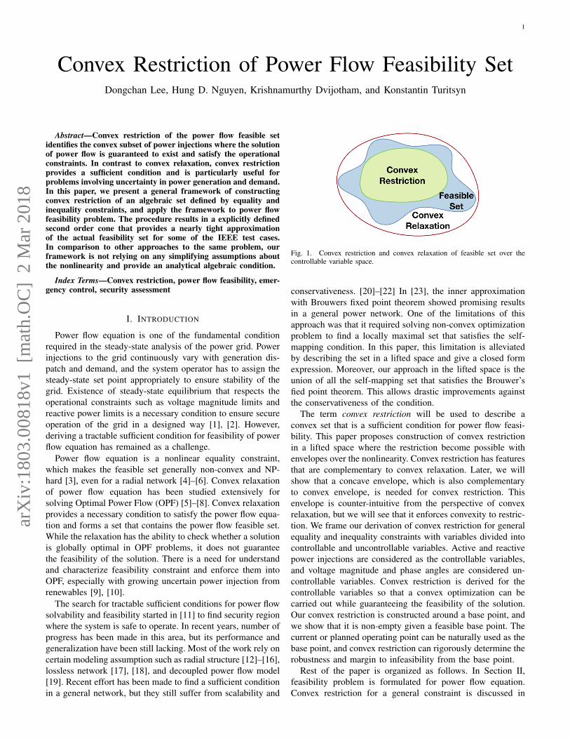
1
Convex Restriction of Power Flow Feasibility SetDongchan Lee, Hung D. Nguyen, Krishnamurthy Dvijotham, and Konstantin Turitsyn
Abstract—Convex restriction of the power flow feasible setidentifies the convex subset of power injections where the solutionof power flow is guaranteed to exist and satisfy the operationalconstraints. In contrast to convex relaxation, convex restrictionprovides a sufficient condition and is particularly useful forproblems involving uncertainty in power generation and demand.In this paper, we present a general framework of constructingconvex restriction of an algebraic set defined by equality andinequality constraints, and apply the framework to power flowfeasibility problem. The procedure results in a explicitly definedsecond order cone that provides a nearly tight approximationof the actual feasibility set for some of the IEEE test cases.In comparison to other approaches to the same problem, ourframework is not relying on any simplifying assumptions aboutthe nonlinearity and provide an analytical algebraic condition.
Index Terms—Convex restriction, power flow feasibility, emer-gency control, security assessment
I. INTRODUCTION
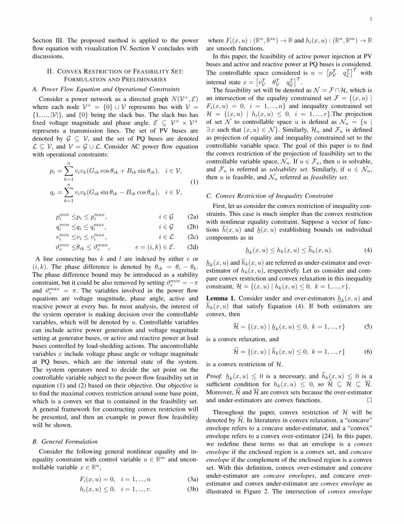
Power flow equation is one of the fundamental conditionrequired in the steady-state analysis of the power grid. Powerinjections to the grid continuously vary with generation dis-patch and demand, and the system operator has to assign thesteady-state set point appropriately to ensure stability of thegrid. Existence of steady-state equilibrium that respects theoperational constraints such as voltage magnitude limits andreactive power limits is a necessary condition to ensure secureoperation of the grid in a designed way [1], [2]. However,deriving a tractable sufficient condition for feasibility of powerflow equation has remained as a challenge.
Power flow equation is a nonlinear equality constraint,which makes the feasible set generally non-convex and NP-hard [3], even for a radial network [4]–[6]. Convex relaxationof power flow equation has been studied extensively forsolving Optimal Power Flow (OPF) [5]–[8]. Convex relaxationprovides a necessary condition to satisfy the power flow equa-tion and forms a set that contains the power flow feasible set.While the relaxation has the ability to check whether a solutionis globally optimal in OPF problems, it does not guaranteethe feasibility of the solution. There is a need for understandand characterize feasibility constraint and enforce them intoOPF, especially with growing uncertain power injection fromrenewables [9], [10].
The search for tractable sufficient conditions for power flowsolvability and feasibility started in [11] to find security regionwhere the system is safe to operate. In recent years, number ofprogress has been made in this area, but its performance andgeneralization have been still lacking. Most of the work rely oncertain modeling assumption such as radial structure [12]–[16],lossless network [17], [18], and decoupled power flow model[19]. Recent effort has been made to find a sufficient conditionin a general network, but they still suffer from scalability and
Fig. 1. Convex restriction and convex relaxation of feasible set over thecontrollable variable space.
conservativeness. [20]–[22] In [23], the inner approximationwith Brouwers fixed point theorem showed promising resultsin a general power network. One of the limitations of thisapproach was that it required solving non-convex optimizationproblem to find a locally maximal set that satisfies the self-mapping condition. In this paper, this limitation is alleviatedby describing the set in a lifted space and give a closed formexpression. Moreover, our approach in the lifted space is theunion of all the self-mapping set that satisfies the Brouwer’sfied point theorem. This allows drastic improvements againstthe conservativeness of the condition.
The term convex restriction will be used to describe aconvex set that is a sufficient condition for power flow feasi-bility. This paper proposes construction of convex restrictionin a lifted space where the restriction become possible withenvelopes over the nonlinearity. Convex restriction has featuresthat are complementary to convex relaxation. Later, we willshow that a concave envelope, which is also complementaryto convex envelope, is needed for convex restriction. Thisenvelope is counter-intuitive from the perspective of convexrelaxation, but we will see that it enforces convexity to restric-tion. We frame our derivation of convex restriction for generalequality and inequality constraints with variables divided intocontrollable and uncontrollable variables. Active and reactivepower injections are considered as the controllable variables,and voltage magnitude and phase angles are considered un-controllable variables. Convex restriction is derived for thecontrollable variables so that a convex optimization can becarried out while guaranteeing the feasibility of the solution.Our convex restriction is constructed around a base point, andwe show that it is non-empty given a feasible base point. Thecurrent or planned operating point can be naturally used as thebase point, and convex restriction can rigorously determine therobustness and margin to infeasibility from the base point.
Rest of the paper is organized as follows. In Section II,feasibility problem is formulated for power flow equation.Convex restriction for a general constraint is discussed in
arX
iv:1
803.
0081
8v1
[m
ath.
OC
] 2
Mar
201
8
2
Section III. The proposed method is applied to the powerflow equation with visualization IV. Section V concludes withdiscussions.
II. CONVEX RESTRICTION OF FEASIBILITY SET:FORMULATION AND PRELIMINARIES
A. Power Flow Equation and Operational Constraints
Consider a power network as a directed graph N(V+, E)where each node V+ = {0} ∪ V represents bus with V ={1, ..., |V|}, and {0} being the slack bus. The slack bus hasfixed voltage magnitude and phase angle. E ⊆ V+ × V+
represents a transmission lines. The set of PV buses aredenoted by G ⊆ V , and the set of PQ buses are denotedL ⊆ V , and V = G ∪ L. Consider AC power flow equationwith operational constraints:
pi =
n∑k=1
vivk(Gik cos θik +Bik sin θik), i ∈ V,
qi =
n∑k=1
vivk(Gik sin θik −Bik cos θik), i ∈ V,(1)
pmini ≤pi ≤ pmaxi , i ∈ G (2a)
qmini ≤qi ≤ qmaxi , i ∈ G (2b)
vmini ≤vi ≤ vmaxi , i ∈ L (2c)
ϑmine ≤θik ≤ ϑmaxe , e = (i, k) ∈ E . (2d)
A line connecting bus k and l are indexed by either e or(i, k). The phase difference is denoted by θik = θi − θk.The phase difference bound may be introduced as a stabilityconstraint, but it could be also removed by setting ϑmine = −πand ϑmaxe = π. The variables involved in the power flowequations are voltage magnitude, phase angle, active andreactive power at every bus. In most analysis, the interest ofthe system operator is making decision over the controllablevariables, which will be denoted by u. Controllable variablescan include active power generation and voltage magnitudesetting at generator buses, or active and reactive power at loadbuses controlled by load-shedding actions. The uncontrollablevariables x include voltage phase angle or voltage magnitudeat PQ buses, which are the internal state of the system.The system operators need to decide the set point on thecontrollable variable subject to the power flow feasibility set inequation (1) and (2) based on their objective. Our objective isto find the maximal convex restriction around some base point,which is a convex set that is contained in the feasibility set.A general framework for constructing convex restriction willbe presented, and then an example in power flow feasibilitywill be shown.
B. General Formulation
Consider the following general nonlinear equality and in-equality constraint with control variable u ∈ Rm and uncon-trollable variable x ∈ Rn,
Fi(x, u) = 0, i = 1, ..., n (3a)hi(x, u) ≤ 0, i = 1, ..., r. (3b)
where Fi(x, u) : (Rn,Rm)→ R and hi(x, u) : (Rn,Rm)→ Rare smooth functions.
In this paper, the feasibility of active power injection at PVbuses and active and reactive power at PQ buses is considered.The controllable space considered is u =
[pTV qTL
]Twith
internal state x =[vTV θTV qTG
]T.
The feasibility set will be denoted as N = F ∩H, which isan intersection of the equality constrained set F = {(x, u) |Fi(x, u) = 0, i = 1, ..., n} and inequality constrained setH = {(x, u) | hi(x, u) ≤ 0, i = 1, ..., r}.The projectionof set N to controllable space u is defined as Nu = {u |∃x such that (x, u) ∈ N}. Similarly, Hu and Fu is definedas projection of equality and inequality constrained set to thecontrollable variable space. The goal of this paper is to findthe convex restriction of the projection of feasibility set to thecontrollable variable space, Nu. If u ∈ Fu, then u is solvable,and Fu is referred as solvability set. Similarly, if u ∈ Nu,then u is feasible, and Nu referred as feasibility set.
C. Convex Restriction of Inequality Constraint
First, let us consider the convex restriction of inequality con-straints. This case is much simpler than the convex restrictionwith nonlinear equality constraint. Suppose a vector of func-tions h(x, u) and h(x, u) establishing bounds on individualcomponents as in
hk(x, u) ≤ hk(x, u) ≤ hk(x, u). (4)
hk(x, u) and hk(x, u) are referred as under-estimator and over-estimator of hk(x, u), respectively. Let us consider and com-pare convex restriction and convex relaxation in this inequalityconstraint, H = {(x, u) | hk(x, u) ≤ 0, k = 1, ..., r}.
Lemma 1. Consider under and over-estimators hk(x, u) andhk(x, u) that satisfy Equation (4). If both estimators areconvex, then
H = {(x, u) | hk(x, u) ≤ 0, k = 1, ..., r} (5)
is a convex relaxation, and
H = {(x, u) | hk(x, u) ≤ 0, k = 1, ..., r} (6)
is a convex restriction of H.
Proof. hk(x, u) ≤ 0 is a necessary, and hk(x, u) ≤ 0 is asufficient condition for hk(x, u) ≤ 0, so H ⊆ H ⊆ H.Moreover, H andH are convex sets because the over-estimatorand under-estimators are convex functions.
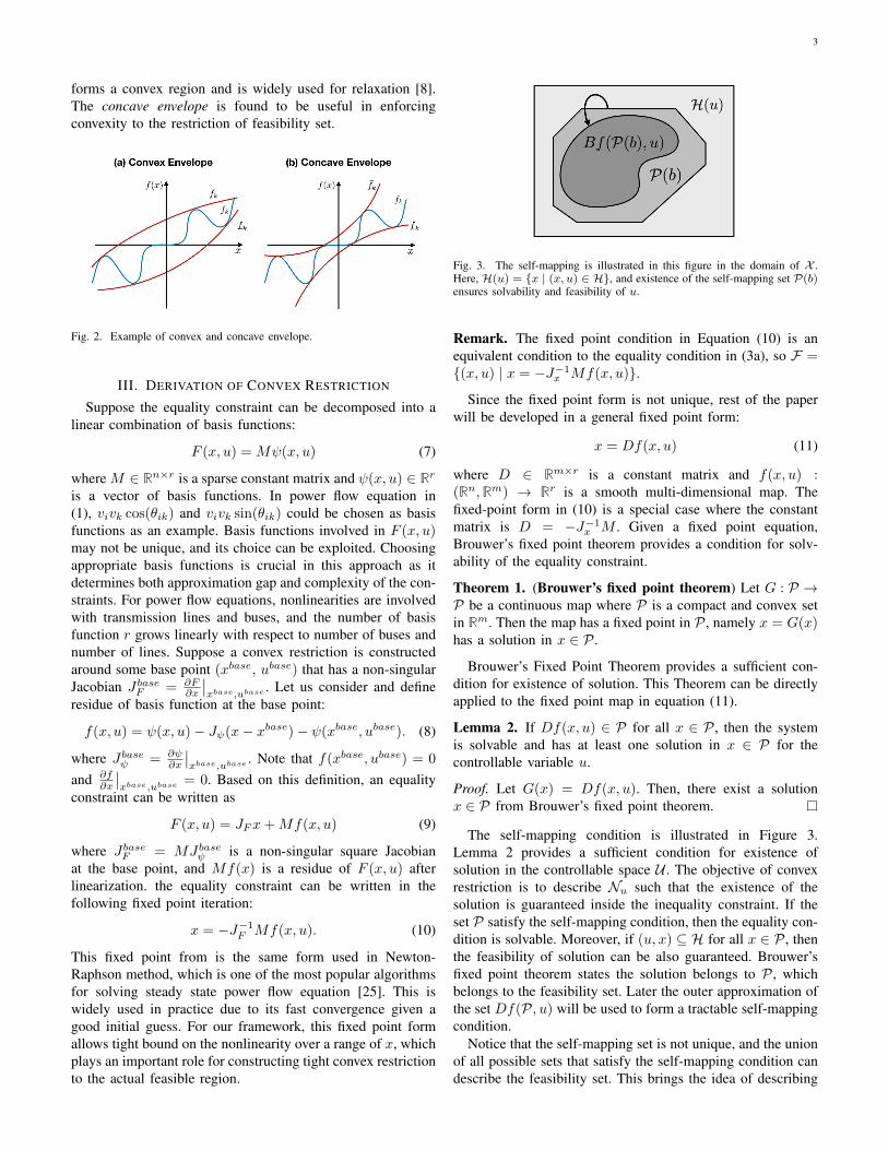
Throughout the paper, convex restriction of H will bedenoted by H. In literatures in convex relaxation, a “concave”envelope refers to a concave under-estimator, and a “convex”envelope refers to a convex over-estimator [24]. In this paper,we redefine these terms so that an envelope is a convexenvelope if the enclosed region is a convex set, and concaveenvelope if the complement of the enclosed region is a convexset. With this definition, convex over-estimator and concaveunder-estimator are concave envelopes, and concave over-estimator and convex under-estimator are convex envelope asillustrated in Figure 2. The intersection of convex envelope
3
forms a convex region and is widely used for relaxation [8].The concave envelope is found to be useful in enforcingconvexity to the restriction of feasibility set.
Fig. 2. Example of convex and concave envelope.
III. DERIVATION OF CONVEX RESTRICTION
Suppose the equality constraint can be decomposed into alinear combination of basis functions:
F (x, u) = Mψ(x, u) (7)
where M ∈ Rn×r is a sparse constant matrix and ψ(x, u) ∈ Rr
is a vector of basis functions. In power flow equation in(1), vivk cos(θik) and vivk sin(θik) could be chosen as basisfunctions as an example. Basis functions involved in F (x, u)may not be unique, and its choice can be exploited. Choosingappropriate basis functions is crucial in this approach as itdetermines both approximation gap and complexity of the con-straints. For power flow equations, nonlinearities are involvedwith transmission lines and buses, and the number of basisfunction r grows linearly with respect to number of buses andnumber of lines. Suppose a convex restriction is constructedaround some base point (xbase, ubase) that has a non-singularJacobian JbaseF = ∂F
∂x
∣∣xbase,ubase . Let us consider and define
residue of basis function at the base point:
f(x, u) = ψ(x, u)− Jψ(x− xbase)− ψ(xbase, ubase). (8)
where Jbaseψ = ∂ψ∂x
∣∣xbase,ubase . Note that f(xbase, ubase) = 0
and ∂f∂x
∣∣xbase,ubase = 0. Based on this definition, an equality
constraint can be written as
F (x, u) = JFx+Mf(x, u) (9)
where JbaseF = MJbaseψ is a non-singular square Jacobianat the base point, and Mf(x) is a residue of F (x, u) afterlinearization. the equality constraint can be written in thefollowing fixed point iteration:
x = −J−1F Mf(x, u). (10)
This fixed point from is the same form used in Newton-Raphson method, which is one of the most popular algorithmsfor solving steady state power flow equation [25]. This iswidely used in practice due to its fast convergence given agood initial guess. For our framework, this fixed point formallows tight bound on the nonlinearity over a range of x, whichplays an important role for constructing tight convex restrictionto the actual feasible region.
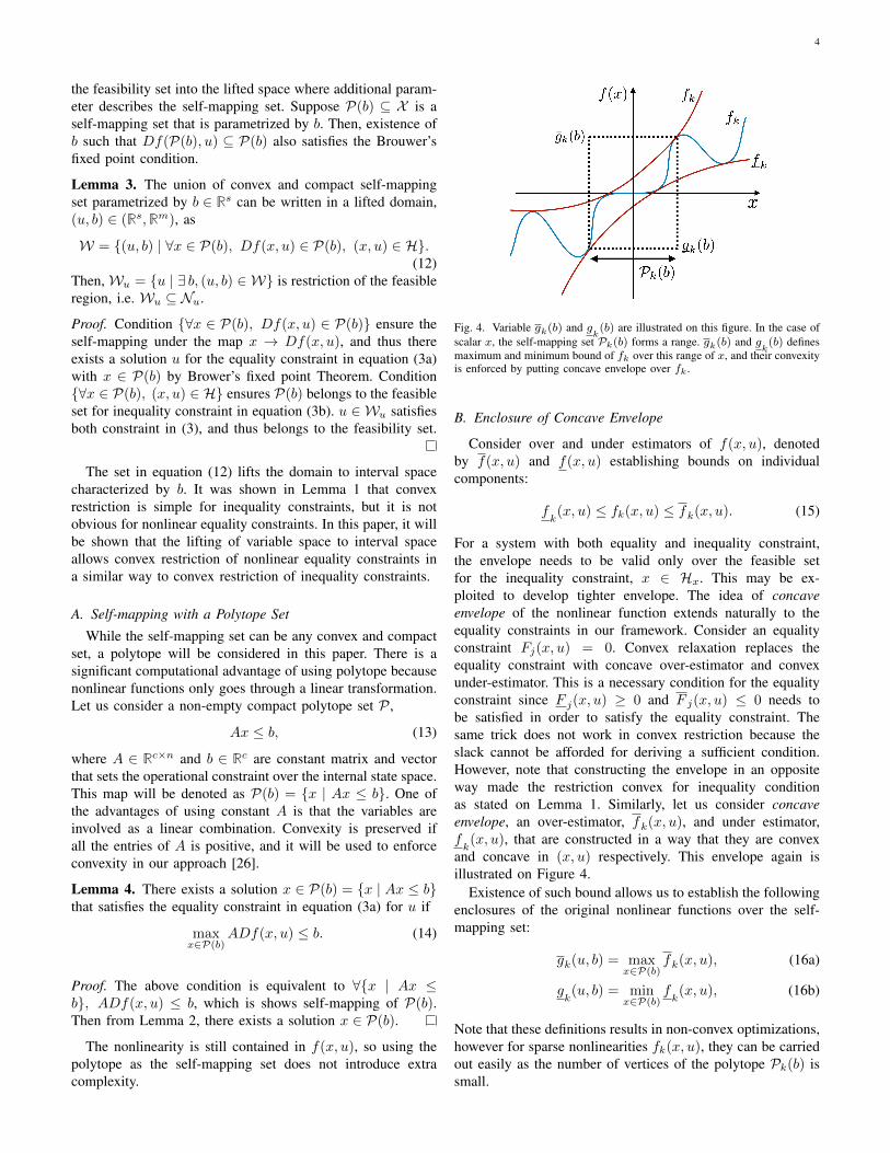
Fig. 3. The self-mapping is illustrated in this figure in the domain of X .Here, H(u) = {x | (x, u) ∈ H}, and existence of the self-mapping set P(b)ensures solvability and feasibility of u.
Remark. The fixed point condition in Equation (10) is anequivalent condition to the equality condition in (3a), so F ={(x, u) | x = −J−1
x Mf(x, u)}.
Since the fixed point form is not unique, rest of the paperwill be developed in a general fixed point form:
x = Df(x, u) (11)
where D ∈ Rm×r is a constant matrix and f(x, u) :(Rn,Rm) → Rr is a smooth multi-dimensional map. Thefixed-point form in (10) is a special case where the constantmatrix is D = −J−1
x M . Given a fixed point equation,Brouwer’s fixed point theorem provides a condition for solv-ability of the equality constraint.
Theorem 1. (Brouwer’s fixed point theorem) Let G : P →P be a continuous map where P is a compact and convex setin Rm. Then the map has a fixed point in P , namely x = G(x)has a solution in x ∈ P .
Brouwer’s Fixed Point Theorem provides a sufficient con-dition for existence of solution. This Theorem can be directlyapplied to the fixed point map in equation (11).
Lemma 2. If Df(x, u) ∈ P for all x ∈ P , then the systemis solvable and has at least one solution in x ∈ P for thecontrollable variable u.
Proof. Let G(x) = Df(x, u). Then, there exist a solutionx ∈ P from Brouwer’s fixed point theorem.
The self-mapping condition is illustrated in Figure 3.Lemma 2 provides a sufficient condition for existence ofsolution in the controllable space U . The objective of convexrestriction is to describe Nu such that the existence of thesolution is guaranteed inside the inequality constraint. If theset P satisfy the self-mapping condition, then the equality con-dition is solvable. Moreover, if (u, x) ⊆ H for all x ∈ P , thenthe feasibility of solution can be also guaranteed. Brouwer’sfixed point theorem states the solution belongs to P , whichbelongs to the feasibility set. Later the outer approximation ofthe set Df(P, u) will be used to form a tractable self-mappingcondition.
Notice that the self-mapping set is not unique, and the unionof all possible sets that satisfy the self-mapping condition candescribe the feasibility set. This brings the idea of describing
4
the feasibility set into the lifted space where additional param-eter describes the self-mapping set. Suppose P(b) ⊆ X is aself-mapping set that is parametrized by b. Then, existence ofb such that Df(P(b), u) ⊆ P(b) also satisfies the Brouwer’sfixed point condition.
Lemma 3. The union of convex and compact self-mappingset parametrized by b ∈ Rs can be written in a lifted domain,(u, b) ∈ (Rs,Rm), as
W = {(u, b) | ∀x ∈ P(b), Df(x, u) ∈ P(b), (x, u) ∈ H}.(12)
Then,Wu = {u | ∃ b, (u, b) ∈ W} is restriction of the feasibleregion, i.e. Wu ⊆ Nu.
Proof. Condition {∀x ∈ P(b), Df(x, u) ∈ P(b)} ensure theself-mapping under the map x → Df(x, u), and thus thereexists a solution u for the equality constraint in equation (3a)with x ∈ P(b) by Brower’s fixed point Theorem. Condition{∀x ∈ P(b), (x, u) ∈ H} ensures P(b) belongs to the feasibleset for inequality constraint in equation (3b). u ∈ Wu satisfiesboth constraint in (3), and thus belongs to the feasibility set.
The set in equation (12) lifts the domain to interval spacecharacterized by b. It was shown in Lemma 1 that convexrestriction is simple for inequality constraints, but it is notobvious for nonlinear equality constraints. In this paper, it willbe shown that the lifting of variable space to interval spaceallows convex restriction of nonlinear equality constraints ina similar way to convex restriction of inequality constraints.
A. Self-mapping with a Polytope Set
While the self-mapping set can be any convex and compactset, a polytope will be considered in this paper. There is asignificant computational advantage of using polytope becausenonlinear functions only goes through a linear transformation.Let us consider a non-empty compact polytope set P ,
Ax ≤ b, (13)
where A ∈ Rc×n and b ∈ Rc are constant matrix and vectorthat sets the operational constraint over the internal state space.This map will be denoted as P(b) = {x | Ax ≤ b}. One ofthe advantages of using constant A is that the variables areinvolved as a linear combination. Convexity is preserved ifall the entries of A is positive, and it will be used to enforceconvexity in our approach [26].
Lemma 4. There exists a solution x ∈ P(b) = {x | Ax ≤ b}that satisfies the equality constraint in equation (3a) for u if
maxx∈P(b)
ADf(x, u) ≤ b. (14)
Proof. The above condition is equivalent to ∀{x | Ax ≤b}, ADf(x, u) ≤ b, which is shows self-mapping of P(b).Then from Lemma 2, there exists a solution x ∈ P(b).
The nonlinearity is still contained in f(x, u), so using thepolytope as the self-mapping set does not introduce extracomplexity.
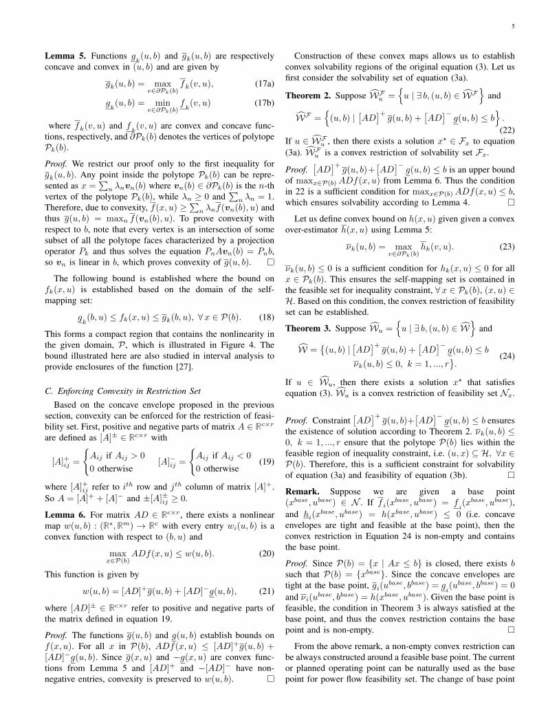
Fig. 4. Variable gk(b) and gk(b) are illustrated on this figure. In the case of
scalar x, the self-mapping set Pk(b) forms a range. gk(b) and gk(b) defines
maximum and minimum bound of fk over this range of x, and their convexityis enforced by putting concave envelope over fk .
B. Enclosure of Concave Envelope
Consider over and under estimators of f(x, u), denotedby f(x, u) and f(x, u) establishing bounds on individualcomponents:
fk(x, u) ≤ fk(x, u) ≤ fk(x, u). (15)
For a system with both equality and inequality constraint,the envelope needs to be valid only over the feasible setfor the inequality constraint, x ∈ Hx. This may be ex-ploited to develop tighter envelope. The idea of concaveenvelope of the nonlinear function extends naturally to theequality constraints in our framework. Consider an equalityconstraint Fj(x, u) = 0. Convex relaxation replaces theequality constraint with concave over-estimator and convexunder-estimator. This is a necessary condition for the equalityconstraint since F j(x, u) ≥ 0 and F j(x, u) ≤ 0 needs tobe satisfied in order to satisfy the equality constraint. Thesame trick does not work in convex restriction because theslack cannot be afforded for deriving a sufficient condition.However, note that constructing the envelope in an oppositeway made the restriction convex for inequality conditionas stated on Lemma 1. Similarly, let us consider concaveenvelope, an over-estimator, fk(x, u), and under estimator,fk(x, u), that are constructed in a way that they are convex
and concave in (x, u) respectively. This envelope again isillustrated on Figure 4.
Existence of such bound allows us to establish the followingenclosures of the original nonlinear functions over the self-mapping set:
gk(u, b) = maxx∈P(b)
fk(x, u), (16a)
gk(u, b) = min
x∈P(b)fk(x, u), (16b)
Note that these definitions results in non-convex optimizations,however for sparse nonlinearities fk(x, u), they can be carriedout easily as the number of vertices of the polytope Pk(b) issmall.
5
Lemma 5. Functions gk(u, b) and gk(u, b) are respectively
concave and convex in (u, b) and are given by
gk(u, b) = maxv∈∂Pk(b)
fk(v, u), (17a)
gk(u, b) = min
v∈∂Pk(b)fk(v, u) (17b)
where fk(v, u) and fk(v, u) are convex and concave func-
tions, respectively, and ∂Pk(b) denotes the vertices of polytopePk(b).
Proof. We restrict our proof only to the first inequality forgk(u, b). Any point inside the polytope Pk(b) can be repre-sented as x =
∑n λnvn(b) where vn(b) ∈ ∂Pk(b) is the n-th
vertex of the polytope Pk(b), while λn ≥ 0 and∑n λn = 1.
Therefore, due to convexity, f(x, u) ≥∑n λnf(vn(b), u) and
thus g(u, b) = maxn f(vn(b), u). To prove convexity withrespect to b, note that every vertex is an intersection of somesubset of all the polytope faces characterized by a projectionoperator Pk and thus solves the equation PnAvn(b) = Pnb,so vn is linear in b, which proves convexity of g(u, b).
The following bound is established where the bound onfk(x, u) is established based on the domain of the self-mapping set:
gk(b, u) ≤ fk(x, u) ≤ gk(b, u), ∀x ∈ P(b). (18)
This forms a compact region that contains the nonlinearity inthe given domain, P , which is illustrated in Figure 4. Thebound illustrated here are also studied in interval analysis toprovide enclosures of the function [27].
C. Enforcing Convexity in Restriction Set
Based on the concave envelope proposed in the previoussection, convexity can be enforced for the restriction of feasi-bility set. First, positive and negative parts of matrix A ∈ Rc×r
are defined as [A]± ∈ Rc×r with
[A]+ij =
{Aij if Aij > 0
0 otherwise[A]−ij =
{Aij if Aij < 0
0 otherwise(19)
where [A]+ij refer to ith row and jth column of matrix [A]+.So A = [A]+ + [A]− and ±[A]±ij ≥ 0.
Lemma 6. For matrix AD ∈ Rc×r, there exists a nonlinearmap w(u, b) : (Rs,Rm) → Rc with every entry wi(u, b) is aconvex function with respect to (b, u) and
maxx∈P(b)
ADf(x, u) ≤ w(u, b). (20)
This function is given by
w(u, b) = [AD]+g(u, b) + [AD]−g(u, b), (21)
where [AD]± ∈ Rc×r refer to positive and negative parts ofthe matrix defined in equation 19.
Proof. The functions g(u, b) and g(u, b) establish bounds onf(x, u). For all x in P(b), ADf(x, u) ≤ [AD]+g(u, b) +[AD]−g(u, b). Since g(x, u) and −g(x, u) are convex func-tions from Lemma 5 and [AD]+ and −[AD]− have non-negative entries, convexity is preserved to w(u, b).
Construction of these convex maps allows us to establishconvex solvability regions of the original equation (3). Let usfirst consider the solvability set of equation (3a).
Theorem 2. Suppose WFu ={u | ∃ b, (u, b) ∈ WF
}and
WF ={
(u, b) |[AD
]+g(u, b) +
[AD
]−g(u, b) ≤ b
}.
(22)If u ∈ WFu , then there exists a solution x? ∈ Fx to equation(3a). WFu is a convex restriction of solvability set Fx.
Proof.[AD
]+g(u, b)+
[AD
]−g(u, b) ≤ b is an upper bound
of maxx∈P(b)ADf(x, u) from Lemma 6. Thus the conditionin 22 is a sufficient condition for maxx∈P(b)ADf(x, u) ≤ b,which ensures solvability according to Lemma 4.
Let us define convex bound on h(x, u) given given a convexover-estimator h(x, u) using Lemma 5:
νk(u, b) = maxv∈∂Pk(b)
hk(v, u). (23)
νk(u, b) ≤ 0 is a sufficient condition for hk(x, u) ≤ 0 for allx ∈ Pk(b). This ensures the self-mapping set is contained inthe feasible set for inequality constraint, ∀x ∈ Pk(b), (x, u) ∈H. Based on this condition, the convex restriction of feasibilityset can be established.
Theorem 3. Suppose Wu ={u | ∃ b, (u, b) ∈ W
}and
W ={
(u, b) |[AD
]+g(u, b) +
[AD
]−g(u, b) ≤ b
νk(u, b) ≤ 0, k = 1, ..., r}.
(24)
If u ∈ Wu, then there exists a solution x? that satisfiesequation (3). Wu is a convex restriction of feasibility set Nx.
Proof. Constraint[AD
]+g(u, b)+
[AD
]−g(u, b) ≤ b ensures
the existence of solution according to Theorem 2. νk(u, b) ≤0, k = 1, ..., r ensure that the polytope P(b) lies within thefeasible region of inequality constraint, i.e. (u, x) ⊆ H, ∀x ∈P(b). Therefore, this is a sufficient constraint for solvabilityof equation (3a) and feasibility of equation (3b).
Remark. Suppose we are given a base point(xbase, ubase) ∈ N . If f i(x
base, ubase) = fi(xbase, ubase),
and hi(xbase, ubase) = h(xbase, ubase) ≤ 0 (i.e. concave
envelopes are tight and feasible at the base point), then theconvex restriction in Equation 24 is non-empty and containsthe base point.
Proof. Since P(b) = {x | Ax ≤ b} is closed, there exists bsuch that P(b) = {xbase}. Since the concave envelopes aretight at the base point, gi(u
base, bbase) = gi(ubase, bbase) = 0
and νi(ubase, bbase) = h(xbase, ubase). Given the base point isfeasible, the condition in Theorem 3 is always satisfied at thebase point, and thus the convex restriction contains the basepoint and is non-empty.
From the above remark, a non-empty convex restriction canbe always constructed around a feasible base point. The currentor planned operating point can be naturally used as the basepoint for power flow feasibility set. The change of base point
6
can be also explored to construct convex restriction around thedesired region.
IV. CONVEX RESTRICTION OF POWER FLOW FEASIBILITYSET
In this section, convex restriction is constructed for ACpower flow equation in polar coordinate. The fixed pointform of the power flow equation is not unique, but the polarrepresentation of power flow equation is chosen. The polarrepresentation includes the voltage magnitude explicitly inthe equation so it is easier to ensure feasibility of voltagemagnitude limits. AC power flow equation in equation (1) canbe written in complex plane as follows:
pi + jqi =∑k
Y Hik vivke−jθik , i ∈ V, (25)
where Yik = Gik + jBik, and Y Hik is a conjugate of Yik.Suppose the feasible base point if provided by θbase and vbase.Let ∆θ = θ− θbase and ∆v = v− vbase. Let the deviation ofphase difference be θik = θbaseik + ∆θik, then
pi + jqi =∑k
(Y Hik e
−jθbaseik
)vivke
−j∆θik , i ∈ V, (26)
where the base point phase is combined with the admittancematrix. This can be expressed with trigonometric functions fori ∈ V ,
pi =∑k∈V\i
vivk(Gik cos ∆ϑe + Bik sin ∆ϑe) + Giiv2i
qi =∑k∈V\i
vivk(Gik sin ∆ϑe − Bik cos ∆ϑe)− Biiv2i ,
(27)
where Gik+jBik = Y Hik e−jθbase
ik and ∆ϑe = ∆θi−∆θk, e =(i, k). The advantage of using equation (27) over (1) is thatthe concave envelope over trigonometric function is tighterand easier to derive when the base point is at the zero of thetrigonometric functions. From the power flow equation, basisfunctions can be recognized by identifying sparse nonlineari-ties,
ψ(x, u) =
pVqL
vfrvto cos ∆ϑvfrvto sin ∆ϑ
v2Lv2G
. (28)
where vfr and vto are voltages at the from and to end oftransmission line respectively. The equality condition overactive power balance at every bus and reactive power balanceat PQ buses will be enforced. Let the uncontrollable variablesbe the deviation of voltage magnitude and phase deviation,x =
[∆θTV ∆vTL
]. The phase at the slack bus is fixed to
zero and the voltage magnitude at PV buses are also fixed.The reactive power balance at PV buses will be placed asthe inequality condition to represent reactive power limit.With the basis function in (28), the equality constraint isF (x, u) = Mψ(x, u) = 0 where
M =
[I|V| 0 −GE+
V −BE−V −GdL −GdG0 I|L| BE+
L −GE−L BdL BdG
](29)
where I|V| ∈ R|V|×|V| is an identity matrix and 0 is a matrixwith zero entries of appropriate size. Moreover,
GE+le =
Gik if l = i
Gik if l = k
0 otherwiseGE−le =
Gik if l = i
−Gik if l = k
0 otherwise(30)
for l ∈ V and e = (i, k) ∈ E . BE± are defined in the same wayby replacing Gik with Bik. Gd and Bd are diagonal matriceswith its diagonal elements equal to diagonals of G and B,respectively. GE+
V denotes selecting only rows i ∈ V fromGE+. Residues of basis functions are computed using equation(8),
f(x, u) =
pV − pbaseVqL − pbaseV
vfrvto(cos ∆ϑ− 1)− vbasefr ∆vto −∆vfrvbaseto
vfrvto sin ∆ϑ− vbasefr vbaseto ∆ϑ
v2L − 2vbaseL ∆vL −
(vbaseL
)20|G|
,(31)
where a product notation is overloaded to element-wise prod-uct. For example, vfrvto cos ∆ϑ is element-wise product ofvfr, vto, and cos ∆ϑ. The operational constraint on the voltagemagnitude and phase can be written as Ax ≤ bmax where
A =
ETV 00 I|L|−ETV 0
0 −I|L|
and bmax =
∆ϑmaxV∆vmaxL−∆ϑminV−∆vminL
(32)
where ∆ϑmin/max = ϑmin/max − ϑbase and ∆vmin/max =vmin/max − vbase. EV is the incidence matrix with columnschosen for only non-slack buses. The reactive power limitconstraint on PV buses can be written as Cf(x, u) ≤ d where
C =
[0 0 −BE+
G GE−G −BdL −BdG0 0 BE+
G −GE−G BdL BdG
](33)
and d =[(∆qmaxG )T −(∆qminG )T
]T. Operational constraint
over the active power at every bus and reactive power at loadbuses will not be considered. These constraints only add upperand lower bound over u, which does not add any interestingfeatures. The inequality constrained set is then H = {(x, u) |Ax ≤ bmax, Cf(x, u) ≤ d}. The matrix A will be also usedfor the self-mapping set, P = {x | Ax ≤ b}. Therefore,P ⊆ H if b ≤ bmax and [C]+g(u, b) + [C]−g(u, b) ≤ d. Thetrigonometric terms and its product with voltage magnitudesare bounded effectively with the phase angle differences andvoltage magnitudes, and tight concave envelopes can be de-rived with such self-mapping set. Quadratic concave envelopeswill be derived for bilinear and trigonometric functions, andthe convex restriction will be constructed as a second ordercone.
A. Quadratic concave envelopeThe main nonlinearities involved in the power flow equation
in polar coordinates are the bilinear, trilinear and trigonomet-ric functions. The concave envelopes of these functions aredeveloped as building blocks.
7
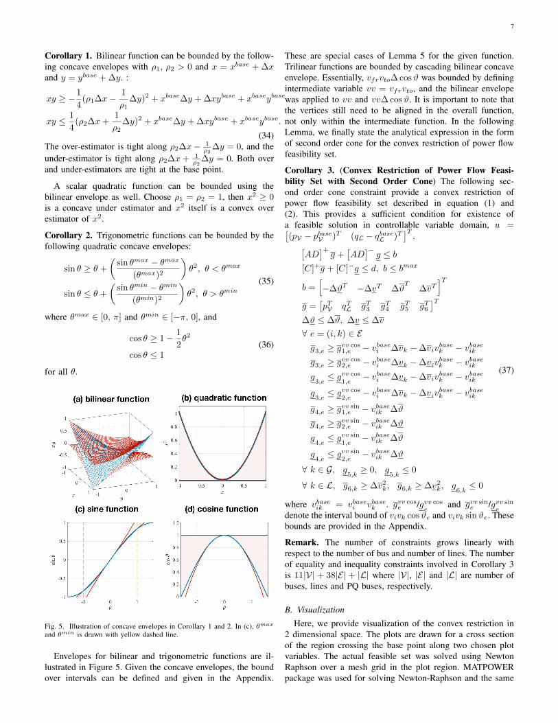
Corollary 1. Bilinear function can be bounded by the follow-ing concave envelopes with ρ1, ρ2 > 0 and x = xbase + ∆xand y = ybase + ∆y. :
xy ≥ −1
4(ρ1∆x− 1
ρ1∆y)2 + xbase∆y + ∆xybase + xbaseybase
xy ≤ 1
4(ρ2∆x+
1
ρ2∆y)2 + xbase∆y + ∆xybase + xbaseybase.
(34)The over-estimator is tight along ρ2∆x− 1
ρ2∆y = 0, and the
under-estimator is tight along ρ2∆x + 1ρ2
∆y = 0. Both overand under-estimators are tight at the base point.
A scalar quadratic function can be bounded using thebilinear envelope as well. Choose ρ1 = ρ2 = 1, then x2 ≥ 0is a concave under estimator and x2 itself is a convex overestimator of x2.
Corollary 2. Trigonometric functions can be bounded by thefollowing quadratic concave envelopes:
sin θ ≥ θ +
(sin θmax − θmax
(θmax)2
)θ2, θ < θmax
sin θ ≤ θ +
(sin θmin − θmin
(θmin)2
)θ2, θ > θmin
(35)
where θmax ∈ [0, π] and θmin ∈ [−π, 0], and
cos θ ≥ 1− 1
2θ2
cos θ ≤ 1(36)
for all θ.
Fig. 5. Illustration of concave envelopes in Corollary 1 and 2. In (c), θmax
and θmin is drawn with yellow dashed line.
Envelopes for bilinear and trigonometric functions are il-lustrated in Figure 5. Given the concave envelopes, the boundover intervals can be defined and given in the Appendix.
These are special cases of Lemma 5 for the given function.Trilinear functions are bounded by cascading bilinear concaveenvelope. Essentially, vfrvto∆ cosϑ was bounded by definingintermediate variable vv = vfrvto, and the bilinear envelopewas applied to vv and vv∆ cosϑ. It is important to note thatthe vertices still need to be aligned in the overall function,not only within the intermediate function. In the followingLemma, we finally state the analytical expression in the formof second order cone for the convex restriction of power flowfeasibility set.
Corollary 3. (Convex Restriction of Power Flow Feasi-bility Set with Second Order Cone) The following sec-ond order cone constraint provide a convex restriction ofpower flow feasibility set described in equation (1) and(2). This provides a sufficient condition for existence ofa feasible solution in controllable variable domain, u =[(pV − pbaseV )T (qL − qbaseL )T
]T.[
AD]+g +
[AD
]−g ≤ b
[C]+g + [C]−g ≤ d, b ≤ bmax
b =[−∆ϑT −∆vT ∆ϑ
T∆vT
]Tg =
[pTV qTL gT3 gT4 gT5 gT6
]T∆ϑ ≤ ∆ϑ, ∆v ≤ ∆v
∀ e = (i, k) ∈ Eg3,e ≥ gvv cos
1,e − vbasei ∆vk −∆vivbasek − vbaseik
g3,e ≥ gvv cos2,e − vbasei ∆vk −∆viv
basek − vbaseik
g3,e≤ gvv cos
1,e− vbasei ∆vk −∆viv
basek − vbaseik
g3,e≤ gvv cos
2,e− vbasei ∆vk −∆viv
basek − vbaseik
g4,e ≥ gvv sin1,e − vbaseik ∆ϑ
g4,e ≥ gvv sin2,e − vbaseik ∆ϑ
g4,e≤ gvv sin
1,e− vbaseik ∆ϑ
g4,e≤ gvv sin
2,e− vbaseik ∆ϑ
∀ k ∈ G, g5,k≥ 0, g
5,k≤ 0
∀ k ∈ L, g6,k ≥ ∆v2k, g6,k ≥ ∆v2
k, g6,k≤ 0
(37)
where vbaseik = vbasei vbasek . gvv cose /gvv cos
eand gvv sin
e /gvv sine
denote the interval bound of vivk cosϑe and vivk sinϑe. Thesebounds are provided in the Appendix.
Remark. The number of constraints grows linearly withrespect to the number of bus and number of lines. The numberof equality and inequality constraints involved in Corollary 3is 11|V| + 38|E| + |L| where |V|, |E| and |L| are number ofbuses, lines and PQ buses, respectively.
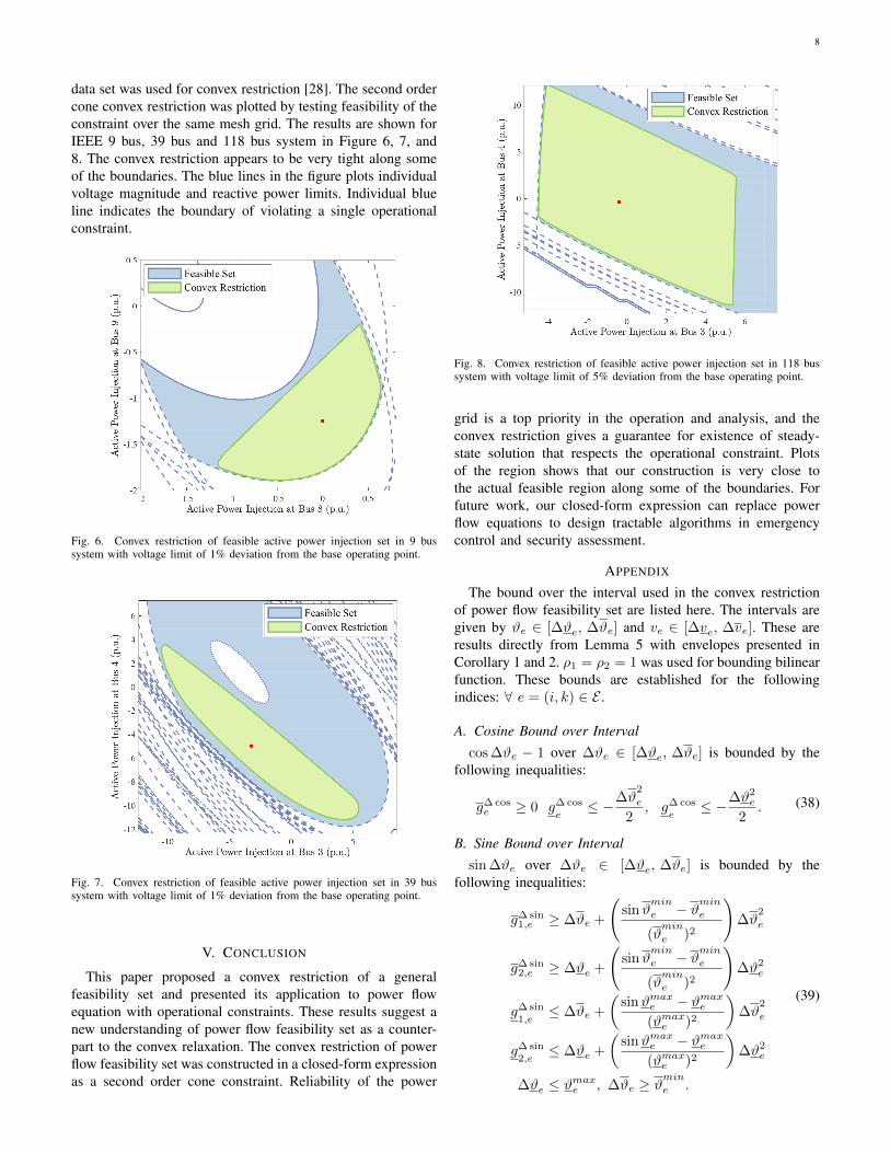
B. Visualization
Here, we provide visualization of the convex restriction in2 dimensional space. The plots are drawn for a cross sectionof the region crossing the base point along two chosen plotvariables. The actual feasible set was solved using NewtonRaphson over a mesh grid in the plot region. MATPOWERpackage was used for solving Newton-Raphson and the same
8
data set was used for convex restriction [28]. The second ordercone convex restriction was plotted by testing feasibility of theconstraint over the same mesh grid. The results are shown forIEEE 9 bus, 39 bus and 118 bus system in Figure 6, 7, and8. The convex restriction appears to be very tight along someof the boundaries. The blue lines in the figure plots individualvoltage magnitude and reactive power limits. Individual blueline indicates the boundary of violating a single operationalconstraint.
Fig. 6. Convex restriction of feasible active power injection set in 9 bussystem with voltage limit of 1% deviation from the base operating point.
Fig. 7. Convex restriction of feasible active power injection set in 39 bussystem with voltage limit of 1% deviation from the base operating point.
V. CONCLUSION
This paper proposed a convex restriction of a generalfeasibility set and presented its application to power flowequation with operational constraints. These results suggest anew understanding of power flow feasibility set as a counter-part to the convex relaxation. The convex restriction of powerflow feasibility set was constructed in a closed-form expressionas a second order cone constraint. Reliability of the power
Fig. 8. Convex restriction of feasible active power injection set in 118 bussystem with voltage limit of 5% deviation from the base operating point.
grid is a top priority in the operation and analysis, and theconvex restriction gives a guarantee for existence of steady-state solution that respects the operational constraint. Plotsof the region shows that our construction is very close tothe actual feasible region along some of the boundaries. Forfuture work, our closed-form expression can replace powerflow equations to design tractable algorithms in emergencycontrol and security assessment.
APPENDIX
The bound over the interval used in the convex restrictionof power flow feasibility set are listed here. The intervals aregiven by ϑe ∈ [∆ϑe, ∆ϑe] and ve ∈ [∆ve, ∆ve]. These areresults directly from Lemma 5 with envelopes presented inCorollary 1 and 2. ρ1 = ρ2 = 1 was used for bounding bilinearfunction. These bounds are established for the followingindices: ∀ e = (i, k) ∈ E .
A. Cosine Bound over Intervalcos ∆ϑe − 1 over ∆ϑe ∈ [∆ϑe, ∆ϑe] is bounded by the
following inequalities:
g∆ cose ≥ 0 g∆ cos
e≤ −∆ϑ
2
e
2, g∆ cos
e≤ −∆ϑ2
e
2. (38)
B. Sine Bound over Intervalsin ∆ϑe over ∆ϑe ∈ [∆ϑe, ∆ϑe] is bounded by the
following inequalities:
g∆ sin1,e ≥ ∆ϑe +
(sinϑ
min
e − ϑmine
(ϑmin
e )2
)∆ϑ
2
e
g∆ sin2,e ≥ ∆ϑe +
(sinϑ
min
e − ϑmine
(ϑmin
e )2
)∆ϑ2
e
g∆ sin1,e
≤ ∆ϑe +
(sinϑmaxe − ϑmaxe
(ϑmaxe )2
)∆ϑ
2
e
g∆ sin2,e
≤ ∆ϑe +
(sinϑmaxe − ϑmaxe
(ϑmaxe )2
)∆ϑ2
e
∆ϑe ≤ ϑmaxe , ∆ϑe ≥ ϑ
min
e .
(39)

9
C. Bilinear Bound over Interval
∆vi∆vk − vbaseik over ∆vi ∈ [∆vi, ∆vi] is bounded by thefollowing inequalities:
g∆vv1,e ≥
1
4(∆vi + ∆vk)2 + vbasei ∆vk + ∆viv
basek
g∆vv2,e ≥
1
4(∆vi + ∆vk)2 + vbasei ∆vk + ∆viv
basek
g∆vv1,e≤ −1
4(∆vi −∆vk)2 + vbasei ∆vk + ∆viv
basek
g∆vv2,e≤ −1
4(∆vi −∆vk)2 + vbasei ∆vk + ∆viv
basek
g∆vve≤ g∆vv
1,e, g∆vv
e≤ g∆vv
2,e
g∆vve ≥ g∆vv
1,e , g∆vve ≥ g∆vv
2,e
(40)
where vbaseik = vbasei vbasek .
D. vivk cos θik Bound over Interval
∆vi∆vk cos θik − vbaseik over ∆vi ∈ [∆vi, ∆vi] and ∆vi ∈[∆vi, ∆vi] is bounded by the following inequalities:
gvv cos1,e ≥ g∆vv
1,e , gvv cos2,e ≥ g∆vv
2,e
gvv cos1,e
≤ −1
4(g∆vve,1− g∆ cos
e)2 + vbaseik g∆ cos
e+ g∆vv
e,1+ vbaseik
gvv cos2,e
≤ −1
4(g∆vve,2− g∆ cos
e)2 + vbaseik g∆ cos
e+ g∆vv
e,2+ vbaseik .
(41)
E. vivk sin θik Bound over Interval
∆vi∆vk sin θik over ∆vi ∈ [∆vi, ∆vi] and ∆vi ∈[∆vi, ∆vi] is bounded by the following inequalities:
gvv sin1,e ≥ 1
4(g∆vve + g∆ sin
1,e )2 + vbaseik g∆ sin1,e
gvv sin2,e ≥ 1
4(g∆vve + g∆ sin
2,e )2 + vbaseik g∆ sin2,e
gvv sin1,e
≤ −1
4(g∆vve− g∆ sin
1,e)2 + vbaseik g∆ sin
1,e
gvv sin2,e
≤ −1
4(g∆vve− g∆ sin
2,e)2 + vbaseik g∆ sin
2,e.
(42)
REFERENCES
[1] T. Van Cutsem and C. Vournas, Voltage stability of electric powersystems. Springer Science & Business Media, 1998, vol. 441.
[2] P. Kundur, N. J. Balu, and M. G. Lauby, Power system stability andcontrol. McGraw-hill New York, 1994, vol. 7.
[3] B. C. Lesieutre and I. A. Hiskens, “Convexity of the set of feasibleinjections and revenue adequacy in ftr markets,” IEEE Transactions onPower Systems, vol. 20, no. 4, pp. 1790–1798, 2005.
[4] K. Lehmann, A. Grastien, and P. Van Hentenryck, “Ac-feasibility ontree networks is np-hard,” IEEE Transactions on Power Systems, vol. 31,no. 1, pp. 798–801, 2016.
[5] S. H. Low, “Convex relaxation of optimal power flow—part i: For-mulations and equivalence,” IEEE Transactions on Control of NetworkSystems, vol. 1, no. 1, pp. 15–27, 2014.
[6] ——, “Convex relaxation of optimal power flow—part ii: Exactness,”IEEE Transactions on Control of Network Systems, vol. 1, no. 2, pp.177–189, 2014.
[7] J. Lavaei and S. H. Low, “Zero duality gap in optimal power flowproblem,” IEEE Transactions on Power Systems, vol. 27, no. 1, pp.92–107, 2012.
[8] C. Coffrin, H. L. Hijazi, and P. Van Hentenryck, “The qc relaxation:A theoretical and computational study on optimal power flow,” IEEETransactions on Power Systems, vol. 31, no. 4, pp. 3008–3018, 2016.
[9] B. Cui and X. A. Sun, “A new voltage stability-constrained optimalpower flow model: Sufficient condition, socp representation, and relax-ation,” arXiv preprint arXiv:1705.10372, 2017.
[10] D. K. Molzahn, “Computing the feasible spaces of optimal power flowproblems,” IEEE Transactions on Power Systems, vol. 32, no. 6, pp.4752–4763, 2017.
[11] F. Wu and S. Kumagai, “Steady-state security regions of power systems,”IEEE Transactions on Circuits and Systems, vol. 29, no. 11, pp. 703–711, 1982.
[12] S. Bolognani and S. Zampieri, “On the existence and linear approxima-tion of the power flow solution in power distribution networks,” IEEETransactions on Power Systems, vol. 31, no. 1, pp. 163–172, 2016.
[13] S. Yu, H. D. Nguyen, and K. S. Turitsyn, “Simple certificate ofsolvability of power flow equations for distribution systems,” in Power& Energy Society General Meeting, 2015 IEEE. IEEE, 2015, pp.1–5.
[14] C. Wang, A. Bernstein, J.-Y. Le Boudec, and M. Paolone, “Explicit con-ditions on existence and uniqueness of load-flow solutions in distributionnetworks,” IEEE Transactions on Smart Grid, 2016.
[15] ——, “Existence and uniqueness of load-flow solutions in three-phasedistribution networks,” IEEE Transactions on Power Systems, vol. 32,no. 4, pp. 3319–3320, 2017.
[16] K. Dvijotham, E. Mallada, and J. W. Simpson-Porco, “High-voltagesolution in radial power networks: Existence, properties, and equivalentalgorithms,” IEEE control systems letters, vol. 1, no. 2, pp. 322–327,2017.
[17] J. W. Simpson-Porco, “A theory of solvability for lossless power flowequations–part i: Fixed-point power flow,” IEEE Transactions on Controlof Network Systems, 2017.
[18] ——, “A theory of solvability for lossless power flow equations–partii: Conditions for radial networks,” IEEE Transactions on Control ofNetwork Systems, 2017.
[19] J. W. Simpson-Porco, F. Dorfler, and F. Bullo, “Voltage collapse incomplex power grids,” Nature communications, vol. 7, p. 10790, 2016.
[20] K. Dvijotham and K. Turitsyn, “Construction of power flow feasibilitysets,” arXiv preprint arXiv:1506.07191, 2015.
[21] K. Dvijotham, H. Nguyen, and K. Turitsyn, “Solvability regions ofaffinely parameterized quadratic equations,” IEEE Control Systems Let-ters, vol. 2, no. 1, pp. 25–30, 2018.
[22] H.-D. Chiang and C.-Y. Jiang, “Feasible region of optimal powerflow: Characterization and applications,” IEEE Transactions on PowerSystems, vol. 33, no. 1, pp. 236–244, 2018.
[23] H. D. Nguyen, K. Dvijotham, and K. Turitsyn, “Inner approximationsof power flow feasibility sets,” arXiv preprint arXiv:1708.06845, 2017.
[24] M. Tawarmalani, J.-P. P. Richard, and C. Xiong, “Explicit convexand concave envelopes through polyhedral subdivisions,” MathematicalProgramming, vol. 138, no. 1-2, pp. 531–577, 2013.
[25] D. Mehta, D. K. Molzahn, and K. Turitsyn, “Recent advances incomputational methods for the power flow equations,” in AmericanControl Conference (ACC), 2016. IEEE, 2016, pp. 1753–1765.
[26] S. Boyd and L. Vandenberghe, Convex optimization. Cambridgeuniversity press, 2004.
[27] R. E. Moore, R. B. Kearfott, and M. J. Cloud, Introduction to intervalanalysis. Siam, 2009, vol. 110.
[28] R. D. Zimmerman, C. E. Murillo-Sanchez, and R. J. Thomas, “Mat-power: Steady-state operations, planning, and analysis tools for powersystems research and education,” IEEE Transactions on power systems,vol. 26, no. 1, pp. 12–19, 2011.