Embed Size (px)
Citation preview

Convex Relaxations for Robust Identification of Hybrid Models
A Dissertation Presented
by
Necmiye Ozay
to
The Department of Electrical and Computer Engineering
in partial fulfillment of the requirements
for the degree of
Doctor of Philosophy
in
Electrical Engineering
Northeastern University
Boston, Massachusetts
July 2010

The dissertation of Necmiye Ozay was read and approved∗ by the following:
Mario Sznaier
Professor of Electrical and Computer Engineering, Northeastern University
Dissertation Adviser
Chair of Committee
Dana H. Brooks
Professor of Electrical and Computer Engineering, Northeastern University
Dissertation Reader
Octavia I. Camps
Professor of Electrical and Computer Engineering, Northeastern University
Dissertation Reader
Constantino M. Lagoa
Professor of Electrical Engineering, The Pennsylvania State University
Dissertation Reader
Gilead Tadmor
Professor of Electrical and Computer Engineering, and Mathematics, Northeastern University
Dissertation Reader
Ali Abur
Professor of Electrical and Computer Engineering, Northeastern University
Department Head
∗ Signatures are on file in the Graduate School.
Abstract
Northeastern University
Department of Electrical and Computer Engineering
Doctor of Philosophy in Electrical Engineering
Convex Relaxations for Robust Identification of Hybrid Models
by Necmiye Ozay
In order to extract useful information from a data set, it is necessary to understand the underlying
model. This dissertation addresses two of the main challenges in identification of such models. First,
the data is often generated by multiple, unknown number of sources; that is, the underlying model is
usually a mixture model or hybrid model. This requires solving the identification and data association
problems simultaneously. Second, the data is usually corrupted by noise necessitating robust identi-
fication schemes. Motivated by these challenges we consider the problem of robust identification of
hybrid models that interpolate the data within a given noise bound. In particular, for static data we try
to fit affine subspace arrangements or more generally a mixture of algebraic surfaces to the data; and
for dynamic data we try to infer the underlying switched affine dynamical system. Clearly, as stated,
these problems admit infinitely many solutions. For instance, one can always find a trivial hybrid
model with as many submodels/subspaces as the number of data points (i.e. one submodel/subspace
per data point). In order to regularize the problem, we define suitable a priori model sets and objec-
tive functions that seek ”simple” models. Although this leads to generically NP-Hard problems, we
develop computationally efficient algorithms based on convex relaxations.
Additionally, we discuss a related problem: robust model (in)validation for affine hybrid systems.
Before a given system description, obtained either from first principles or an identification step, can be
used to design controllers, it must be validated using additional experimental data. In this dissertation,
we show that the invalidation problem for switched affine systems can be solved within a similar
framework by exploiting a combination of elements from convex analysis and the classical theory of
moments.
Finally, the effectiveness of the proposed methods are illustrated using both simulations and several
non-trivial applications in computer vision such as video and dynamic texture segmentation, two-view
motion segmentation and human activity analysis. In all cases the proposed methods significantly
outperform existing approaches both in terms of accuracy and resilience to noise.

Acknowledgements
First and foremost, I would like to thank my adviser, Professor Mario Sznaier for his support in all
aspects of my graduate life. His guidance, encouragement and enthusiasm made this journey quite fun
for me. I am especially thankful to him for giving me the independence to pursue my own research
ideas but also being there with “crazy” ideas whenever I got stuck. His being a great teacher, technical
expertise, attention to mathematical rigor and broad vision have been and will be a constant source of
inspiration for me.
I would like to thank Professor Octavia Camps who introduced me to the fields of computer vision
and pattern recognition. Her expertise and suggestions have been very useful in finding interesting
computer vision applications for hybrid system identification algorithms developed in this dissertation.
I would also like to express my gratitude to Professor Constantino Lagoa of Penn State. My research
has benefited a lot from discussions and interactions with him.
I am very grateful to Professor Dana Brooks and Professor Gilead Tadmor for serving on my disser-
tation committee and for their insightful comments on my work. I would also like to thank Professor
Brooks for letting me sit in his group meetings.
I feel very fortunate to meet with great friends during my graduate studies. I had a very pleasant start
to my studies in the U.S. thanks to two special friends, Roberto Lublinerman and Dimitris Zarpalas
who have been a great source of support and encouragement. I would also like to thank my lab mates
at the Robust Systems Laboratory at Northeastern for their help and support, and for all the fun times
we spent together chatting about this and that (and sometimes about research). In particular, Mustafa
Ayazoglu helped generating some of the simulation data and figures in this dissertation (he can even
print videos on an eps file). My thanks also go to the CDSP gang and Ms. Joan Pratt for their
friendship, the pizza parties and the wonderful times with the dragonboat team (go go go Huskies!!).
I am also grateful to Sila Kurugol not only for being a very close friend but also for our collaboration
on medical image segmentation.
I want to take this opportunity to thank my professors and teachers back in Turkey for providing me
with a solid education and background. I would also like to thank my closest friends, particularly
Bahar, Dilek and Gugu, for being next to me whenever I need, despite the physical distance.
Finally, my greatest appreciation goes to my family, especially to my parents Kafiye and Hami for
their endless love and support, and for being on the other end of the webcam each and every day.
iii

Contents
Abstract ii
Acknowledgements iii
List of Figures vii
List of Tables ix
Abbreviations x
Symbols xi
1 Introduction 1
1.1 Contributions and Outline . . . . . . . . . . . . . . . . . . . . . . . . . . . . . . . . . 3
2 Convex Relaxations 5
2.1 Background Results on Sparsification . . . . . . . . . . . . . . . . . . . . . . . . . . 6
2.1.1 Sparse Signal Recovery . . . . . . . . . . . . . . . . . . . . . . . . . . . . . 6
2.1.2 Matrix Rank Minimization . . . . . . . . . . . . . . . . . . . . . . . . . . . . 8
2.2 The Problem of Moments and Polynomial Optimization . . . . . . . . . . . . . . . . . 10
2.2.1 The Problem of Moments . . . . . . . . . . . . . . . . . . . . . . . . . . . . 10
2.2.1.1 One Dimensional Case . . . . . . . . . . . . . . . . . . . . . . . . 10
2.2.1.2 Multi-Dimensional Case . . . . . . . . . . . . . . . . . . . . . . . . 11
2.2.2 Polynomial Optimization via Moments . . . . . . . . . . . . . . . . . . . . . 14
2.2.2.1 Exploiting the Sparse Structure . . . . . . . . . . . . . . . . . . . . 15
3 Identification of a Class of Hybrid Dynamical Systems 17
3.1 Introduction and Motivation . . . . . . . . . . . . . . . . . . . . . . . . . . . . . . . 17
3.2 Definitions . . . . . . . . . . . . . . . . . . . . . . . . . . . . . . . . . . . . . . . . . 19
3.3 Problem Statement . . . . . . . . . . . . . . . . . . . . . . . . . . . . . . . . . . . . 20
iv

Contents v
3.4 A Sparsification Approach . . . . . . . . . . . . . . . . . . . . . . . . . . . . . . . . 21
3.4.1 Main Results . . . . . . . . . . . . . . . . . . . . . . . . . . . . . . . . . . . 21
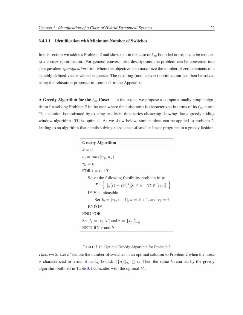
3.4.1.1 Identification with Minimum Number of Switches . . . . . . . . . . 22
A Greedy Algorithm for the ℓ∞ Case: . . . . . . . . . . . . . . . . . . 22
Identifiability of the Switches and Convergence of the Greedy Algorithm: 23
The Case of General Convex Noise Descriptions: . . . . . . . . . . . . 26
Extension to Multi-input Multi-output Models: . . . . . . . . . . . . . 27
Extension to Multidimensional Models: . . . . . . . . . . . . . . . . . 28
3.4.1.2 Identification with Minimum Number of Submodels: . . . . . . . . 29
3.4.2 Examples . . . . . . . . . . . . . . . . . . . . . . . . . . . . . . . . . . . . . 31
3.4.3 Applications: Segmentation of Video Sequences. . . . . . . . . . . . . . . . . 40
Video-Shot Segmentation: . . . . . . . . . . . . . . . . . . . . . . . . 41
Dynamic Textures: . . . . . . . . . . . . . . . . . . . . . . . . . . . . 42
3.5 A Moments-Based Convex Optimization Approach . . . . . . . . . . . . . . . . . . . 43
3.5.1 Main Results . . . . . . . . . . . . . . . . . . . . . . . . . . . . . . . . . . . 46
3.5.1.1 A Moments Based Convex Relaxation: . . . . . . . . . . . . . . . . 46
3.5.2 Illustrative Examples . . . . . . . . . . . . . . . . . . . . . . . . . . . . . . . 50
3.5.2.1 Academic Example: . . . . . . . . . . . . . . . . . . . . . . . . . . 50
3.5.2.2 A Practical Example: Human Activity Segmentation: . . . . . . . . 51
4 Model (In)validation for a Class of Hybrid Dynamical Systems 56
4.1 Introduction and Motivation . . . . . . . . . . . . . . . . . . . . . . . . . . . . . . . 56
4.2 (In)validating MIMO SARX Models . . . . . . . . . . . . . . . . . . . . . . . . . . . 57
4.2.1 Problem Statement . . . . . . . . . . . . . . . . . . . . . . . . . . . . . . . . 58
4.2.2 A Convex Certificate for (In)validating MIMO SARX Models . . . . . . . . . 58
4.3 Numerical Considerations . . . . . . . . . . . . . . . . . . . . . . . . . . . . . . . . 62
4.4 Illustrative Examples . . . . . . . . . . . . . . . . . . . . . . . . . . . . . . . . . . . 64
4.4.1 Academic Examples . . . . . . . . . . . . . . . . . . . . . . . . . . . . . . . 64
4.4.2 A Practical Example: Activity Monitoring . . . . . . . . . . . . . . . . . . . . 66
4.5 Conclusions . . . . . . . . . . . . . . . . . . . . . . . . . . . . . . . . . . . . . . . . 67
5 Clustering Data into Multiple Unknown Subspaces 69
5.1 Sequential Sparsification for Change Detection . . . . . . . . . . . . . . . . . . . . . 70
5.1.1 Introduction and Motivation . . . . . . . . . . . . . . . . . . . . . . . . . . . 70
5.1.2 Segmentation via Sparsification . . . . . . . . . . . . . . . . . . . . . . . . . 71
5.1.3 Applications . . . . . . . . . . . . . . . . . . . . . . . . . . . . . . . . . . . 73
5.1.3.1 Video Segmentation: . . . . . . . . . . . . . . . . . . . . . . . . . . 73
5.1.3.2 Segmentation of Dynamic Textures: . . . . . . . . . . . . . . . . . 74
5.1.4 Experiments . . . . . . . . . . . . . . . . . . . . . . . . . . . . . . . . . . . 74
5.1.4.1 Video Segmentation: . . . . . . . . . . . . . . . . . . . . . . . . . . 74
5.1.4.2 Temporal Segmentation of Dynamic Textures: . . . . . . . . . . . . 76
5.2 GPCA with Denoising: A Moments-Based Convex Approach . . . . . . . . . . . . . . 80

Contents vi
5.2.1 Introduction and Motivation . . . . . . . . . . . . . . . . . . . . . . . . . . . 80
5.2.2 Problem Statement . . . . . . . . . . . . . . . . . . . . . . . . . . . . . . . . 82
5.2.3 Main Results . . . . . . . . . . . . . . . . . . . . . . . . . . . . . . . . . . . 83
5.2.3.1 A Convex Relaxation . . . . . . . . . . . . . . . . . . . . . . . . . 85
5.2.3.2 Extension to Quadratic Surfaces . . . . . . . . . . . . . . . . . . . 87
5.2.3.3 Handling Outliers . . . . . . . . . . . . . . . . . . . . . . . . . . . 88
5.2.4 Experiments . . . . . . . . . . . . . . . . . . . . . . . . . . . . . . . . . . . 89
5.2.4.1 Synthetic Data . . . . . . . . . . . . . . . . . . . . . . . . . . . . . 89
5.2.4.2 2-D motion Estimation and Segmentation . . . . . . . . . . . . . . 91
5.2.4.3 Two View Perspective Motion Segmentation . . . . . . . . . . . . . 93
6 Conclusions and Future Work 96
A Sparsity Related Proofs 98
A.1 Proof of Lemma 1 . . . . . . . . . . . . . . . . . . . . . . . . . . . . . . . . . . . . . 98
A.2 Proof of Lemma 2 . . . . . . . . . . . . . . . . . . . . . . . . . . . . . . . . . . . . . 99
B Recovering the Parameters of the Model in GPCA 102
Bibliography 104
Vita 112
List of Publications 113
List of Figures
3.1 True and estimated parameter sequences for parameter a1(σt) for Example 3. . . . . . 34
3.2 Each histogram shows the frequency of estimated number of submodels for different
noise levels. (a) ǫ = 0.05, (b) ǫ = 0.1, (c) ǫ = 0.25, (d) ǫ = 0.5. The true number of
submodels is s = 3. . . . . . . . . . . . . . . . . . . . . . . . . . . . . . . . . . . . 35
3.3 Median of parameter estimation error ∆n versus noise level ǫ. Error bars indicate the
median absolute deviation. . . . . . . . . . . . . . . . . . . . . . . . . . . . . . . . . 38
3.4 Results for detecting switches in a 2-D system. Left: Original segmentation (i.e. σi,j).
Middle: Output of the system in (3.28). Difference in frequency content of output
values corresponding to the two different submodels can be inferred from the texture.
Right: Resulting segmentation. . . . . . . . . . . . . . . . . . . . . . . . . . . . . . . 39
3.5 Results for detecting switches (i.e. estimating σi,j) in a texture image. Left: Original
image. Middle: GPCA segmentation. Right: Segmentation via proposed method. . . . 40
3.6 Video Segmentation Results. Left Column: Ground truth segmentation (jumps cor-
respond to cuts and slanted lines correspond to gradual transitions). Right Column:
Changes detected with different methods. Value 0 corresponds to frames within a
segment and value 1 corresponds to the frames in transitions. . . . . . . . . . . . . . . 42
3.7 Sample dynamic texture patches. Top: smoke, Bottom: river . . . . . . . . . . . . . . 43
3.8 Results for detecting change in dynamics only. Top: Smoke sequence concatenated
with transposed dynamics. Bottom: River sequence concatenated with reversed dy-
namics. . . . . . . . . . . . . . . . . . . . . . . . . . . . . . . . . . . . . . . . . . . 44
3.9 Clustering via GPCA. . . . . . . . . . . . . . . . . . . . . . . . . . . . . . . . . . . . 51
3.10 Clustering via moments-based method. . . . . . . . . . . . . . . . . . . . . . . . . . . 52
3.11 Absolute error for GPCA identification. . . . . . . . . . . . . . . . . . . . . . . . . . 53
3.12 Absolute error for moments-based identification. . . . . . . . . . . . . . . . . . . . . 54
3.13 Sample frames from the video. . . . . . . . . . . . . . . . . . . . . . . . . . . . . . . 54
3.14 Activity segmentation via GPCA. . . . . . . . . . . . . . . . . . . . . . . . . . . . . 55
3.15 Activity segmentation via moments-based method. . . . . . . . . . . . . . . . . . . . 55
4.1 Problem Setup. The coefficient matrices of the submodels Gi and a bound on the noise
are known a priori. The experimental data consists of input/output measurements, u
and y. The mode signal σt and noise sequence η are unknown. . . . . . . . . . . . . . 59
4.2 Training sequence used in identification of the submodel (A1) for walking. . . . . . . . 67
vii
List of Figures viii
4.3 Top row: Walk, wait, walk sequence (not invalidated). Second row: Running sequence
(invalidated). Third row: Walk, jump sequence (invalidated). Last row: Jumping
sequence (invalidated). . . . . . . . . . . . . . . . . . . . . . . . . . . . . . . . . . . 68
5.1 Video Segmentation Results. First and third row: Ground truth segmentation. Second
and last row: Changes detected with different methods. Value 0 corresponds to frames
within a segment and value 1 corresponds to the frames in transitions. . . . . . . . . . 77
5.2 Sample dynamic texture patches. From left to right: water, flame, steam. . . . . . . . . 78
5.3 Results for detecting change in dynamics only. Top: Smoke sequence concatenated
with transposed dynamics. Bottom: River sequence concatenated with reversed dy-
namics. . . . . . . . . . . . . . . . . . . . . . . . . . . . . . . . . . . . . . . . . . . 79
5.4 An image pair with 3 relocated objects with noisy correspondences superimposed. . . . 80
5.5 Sample segmentation results and mean misclassification rates. (a): GPCA segmenta-
tion (mean misclassification rate: 31.1%). (b): RGPCA segmentation (mean misclas-
sification rate 14.9%). (c): Proposed algorithm (mean misclassification rate 3.7%).
The image size is 600 × 800 and the noise level is ±10 pixels. . . . . . . . . . . . . . 81
5.6 Example using synthetic data laying on two planes in R3. Here the red stars and blue
plus signs indicate the original (noisy) and the denoised data points, respectively. . . . 91
5.7 Fitting errors for GPCA, RGPCA and moments-based methods for the example in
Fig. 5.6. . . . . . . . . . . . . . . . . . . . . . . . . . . . . . . . . . . . . . . . . . . 92
5.8 Example using synthetic data lying on two lines (blue and green) and a plane (trans-
parent red) in R3. Here the red stars and blue plus signs indicate the original (noisy)
and the denoised data points, respectively. . . . . . . . . . . . . . . . . . . . . . . . . 93
5.9 Example using synthetic data lying on two planes in R3. Here the red stars and blue
plus signs indicate the original (noisy) and the denoised data points, respectively. Cyan
circles indicate the points identified as outliers. . . . . . . . . . . . . . . . . . . . . . 94
5.10 Two perspective images of points on teapot surfaces. . . . . . . . . . . . . . . . . . . 95
5.11 (a)-(b) First and second images with moments-based segmentation superimposed, 10
misclassified points. (c) Segmentation with the method in [1], 29 misclassified points. . 95
5.12 (a)-(b) First and second images with moments-based segmentation superimposed (
9.06% misclassification rate). (c) Segmentation with the method in [1] (42.90% mis-
classification rate). . . . . . . . . . . . . . . . . . . . . . . . . . . . . . . . . . . . . 95
List of Tables
3.1 Optimal Greedy Algorithm for Problem 2 . . . . . . . . . . . . . . . . . . . . . . . . 22
3.2 Algorithm for Problem 3 . . . . . . . . . . . . . . . . . . . . . . . . . . . . . . . . . 30
3.3 Minimum number of submodel estimation error statistics for different noise levels.
The results for sparsification is given both with formulation (3.23) and with formula-
tion (3.24) in parantheses. . . . . . . . . . . . . . . . . . . . . . . . . . . . . . . . . . 36
3.4 Normalized parameter identification error statistics of minimum number of submodels
problem with different noise level. The results for sparsification is given both with
formulation (3.23) and with formulation (3.24) in parantheses. . . . . . . . . . . . . . 37
3.5 Rand Indices that show the quality of mode signal estimates. . . . . . . . . . . . . . . 37
3.6 Error measure ∆n that shows the quality of parameter estimates. . . . . . . . . . . . . 38
3.7 Rand indices for video-shot segmentation . . . . . . . . . . . . . . . . . . . . . . . . 41
3.8 Estimated and true values of parameters . . . . . . . . . . . . . . . . . . . . . . . . . 51
4.1 Invalidation results for example 2. The values of p were respectively −3.8441e−008,
−8.2932e − 009, 0.8585, −5.4026e − 008, −1.5490e − 007 and 0.7566. . . . . . . . 65
4.2 Invalidation results for example 3. The values of p were respectively 0.0724, 0.0035,
−5.1810e − 007, 0.0737, 0.0034 and −1.4930e − 007. . . . . . . . . . . . . . . . . . 65
4.3 Invalidation results for example 4. The values of p were ,respectively, 0.8963, 0.0997,
0.0080, 0.0308, 2.8638e − 004, 2.9069e − 006 and 6.2061e − 006. . . . . . . . . . . 65
4.4 Invalidation results for activity monitoring. The values of p were, respectively, −2.3303e−008, 2.3707e − 005, 5.0293e − 007, and 1.5998e − 006. . . . . . . . . . . . . . . . . 67
5.1 Rand indices . . . . . . . . . . . . . . . . . . . . . . . . . . . . . . . . . . . . . . . . 76
5.2 Results on Dynamic Texture Database . . . . . . . . . . . . . . . . . . . . . . . . . . 78
5.3 Synthetic Data Results. D and dk denote the dimension of the ambient space and
subspaces, respectively. N shows the number of samples per subspace. ǫ denotes the
true noise level. The last three columns show the mean and median (in parenthesis)
fitting errors. . . . . . . . . . . . . . . . . . . . . . . . . . . . . . . . . . . . . . . . 90
5.4 Misclassification rates for perspective motion segmentation examples. . . . . . . . . . 94
ix

Abbreviations
ARX Auto-Regressive Exogenous
SARX Switched Affine Auto-Regressive Exogenous
LCCDE Linear Constant Coefficient Difference Equation
ASCDE Affine Switched Coefficient Difference Equation
SISO Single-Input Single-Output
MIMO Multi-Input Multi-Output
LMI Linear Matrix Inequality
SVD Singular Value Decomposition
PCA Principal Component Analysis
GPCA Generalized Principal Component Analysis
RGPCA Robust Generalized Principal Component Analysis
HQSA Hybrid Quadratic Surface Analysis
LP Linear Programming
SDP Semi-definite Programming
NP Non-deterministic Polynomial-time
SOS Sum of Squares
x

Symbols
R, Z set of real numbers, integers
x a vector in RN
M a matrix in Rn×m
‖x‖p p-norm in RN , that is ‖x‖p
.= p
√
∑Ni=1 xp
i
‖x‖∞ ∞-norm of the vector x ∈ RN , that is ‖x‖∞
.= supi |xi|
{x(t)}Tt=1,{x} a vector valued sequence of length T where each x(t) ∈ R
N
‖{x}‖p ℓp norm of a vector valued sequence ‖{x}‖p.=(
∑Ti=1 ‖x(i)‖p
p
)1/p
‖{x}‖0 ℓo-quasinorm.= number of non-zero vectors in the sequence (i.e. cardinality of the
set {t ∈ Z|x(t) 6= 0, t ∈ [1, T ]})
I identity matrix of appropriate dimension
traceM trace of the matrix M
M � N the matrix M− N is positive semidefinite.
R[x1, . . . , xn] the ring of polynomials in n variables over R. R[x] may be used when n is clear
from the context.
Nn positive integers up to n, i.e. Nn.= {1, . . . , n}
∧ (∨) logical AND (OR)
< M,N > trace(MT N)
PnD set of nth degree multivariate polynomials in D variables. n and D may be omitted
when clear from the context.
xi

To my parents, Kafiye and Hami
xii

Chapter 1
Introduction
Hybrid models are abundant in a wide range of applications and processes. In dynamical systems
community hybrid systems, systems characterized by the interaction of both continuous and discrete
dynamics, have been the subject of considerable attention during the past decade. These systems arise
naturally in many different contexts, e.g. biological systems ([2, 3], etc.), systems incorporating logi-
cal and continuous elements ([4, 5]), manufacturing ([6]), automotive ([7]), etc, and in addition, affine
hybrid systems can be used to approximate nonlinear dynamics. Computer vision and pattern recogni-
tion communities have also extensively considered subspace arrangements ([8, 9, 10, 11]) and mixture
models ([12, 13, 14]) in various segmentation/clustering applications such as affine motion segmenta-
tion, face clustering under varying illumination, image, video and dynamic texture segmentation.
In this dissertation, we consider the problem of parametric identification of hybrid models. In partic-
ular, for dynamic input/output data we try to infer the underlying switched affine dynamical system
(i.e. a time–varying system that switches among a finite number of linear time invariant subsystems
according to a discrete mode signal); and for static data we try to fit a union of affine subspaces (i.e.
affine subspace arrangement) or more generally a mixture of algebraic surfaces to the data. The main
challenge in both problems is that one needs to solve the identification and data association problems
simultaneously. For switched affine dynamical systems, if we knew the mode signal (i.e. we knew
which submodel was active at which time instants), then we can treat the problem as the identification
of linear time–invariant systems. Conversely, if we knew the parameters of the submodels, then we
could use model invalidation techniques to find which model is valid for each time instant. Similarly
for static data, if we knew which data points came from the same subspace, then we could easily fit
a subspace to those points. On the other hand if the subspaces were known, each data point could
1
Chapter 1. Introduction 2
be assigned to the subspace closest to it. Identification of hybrid models is a hard problem mainly
due to this chicken-and-egg nature. Moreover, taking into account the fact that the data is usually
corrupted by noise makes the problem even more challenging. We try to address these challenges with
the proposed robust identification schemes.
Also, unless additional constraints are imposed, the identification problem admits infinitely many
solutions. For instance, one can always find a trivial hybrid model with as many submodels/subspaces
as the number of data points (i.e. one submodel/subspace per data point). In order to regularize the
problem, we define suitable a priori model sets and objective functions that seek “simple” models.
Hence, we recast the problem into an optimization form. Although this leads to generically non-convex
NP-Hard problems, we develop computationally efficient algorithms based on convex relaxations.
Convex optimization problems constitute a special class of mathematical optimization problems for
which there are efficient polynomial time algorithms that are guaranteed to converge1 to a global
optimum [15]. Convex relaxations can be used to approximate (in some cases, even exactly solve
for) the global optimum of a non-convex problem in a principled way. With this in mind, we try to
convexify our problems and make use of the powerful tools developed for convex optimization.
We also consider a related problem: robust model (in)validation for affine hybrid systems. Before a
given system description, obtained either from first principles or an identification step, can be used to
design controllers, it must be validated using additional experimental data. Considering the inherent
difficulties in hybrid system identification, an invalidation step becomes even more crucial for such
systems. We show that the invalidation problem for switched affine systems can be solved within a
similar framework by exploiting a combination of elements from convex analysis and the classical
theory of moments.
In addition to developing hybrid identification and (in)validation schemes, we show that many in-
teresting problems in computer vision can be robustly and efficiently solved within a hybrid iden-
tification/(in)validation framework. In particular, we apply the proposed methods in video and dy-
namic/static texture segmentation, two-view motion segmentation and human activity analysis. In all
cases the proposed methods significantly outperform existing approaches both in terms of accuracy
and resilience to noise.
1More precisely, one can get a solution arbitrarily close to the global optimum, in polynomial time.
Chapter 1. Introduction 3
1.1 Contributions and Outline
The main contributions of this dissertation are:
• Reformulation of the problems of identification of switched ARX systems with minimum num-
ber of switches and minimum number of submodels as sparsification problems, making a con-
nection between sparse signal recovery and hybrid system identification. This reformulation
enables efficient convex optimization based solution methods.
• An exact switch detection algorithm for SARX systems with ℓ∞ bounded noise. A notion of
switch identifiability is presented together with necessary and sufficient conditions for identifi-
ability of switches purely from input/output data.
• Derivation of the convex envelop for the function that counts the nonzeros vectors in a vec-
tor valued sequences which lead to a convex relaxation for sparsity problems involving vector
valued sequences.
• Reformulation of identification of switched ARX systems with known number of submodels
and ℓ∞ bounded noise as a matrix rank minimization problem where all the matrices involved
are affine in decision variables. This problem can be solved by using efficient convex relaxations
for rank minimization.
• An extension of moment-based polynomial optimization method for the case where the function
to be minimized is not a polynomial function (i.e. rank). In hybrid system identification problem
considered, keeping the rank objective instead of a more complicated equivalent polynomial
objective function, it is possible to better utilize the problem structure to significantly reduce the
computational complexity.
• Convex certificates for robust (in)validation of multi-input multi-output SARX models and re-
casting activity monitoring problem as a hybrid model invalidation problem.
• Application of hybrid system identification to several non-trival problems in computer vision
establishing the fact that hybrid dynamical models provide a compact representation for complex
data streams that are generated by multiple sources or for which the underlying process varies
with time. Also in all cases, the proposed approaches are shown to outperform the state-of-the-
art techniques currently used in the computer vision field.

Chapter 1. Introduction 4
• A sparsification based method, which takes into account the order dependency, for clustering
noise corrupted data that lie on a mixture of subspaces and its applications in video and dynamic
texture segmentation.
• A moments-based convex method for segmentation of multiple algebraic surfaces from noisy
sample data points. This method is applied to the problems of simultaneous 2-D two view mo-
tion segmentation and motion segmentation from two perspective views. Simulations and real
examples illustrate that our formulation substantially reduces the noise sensitivity of existing
approaches.
The rest of the dissertation is organized as follows. We start with a summary of convex relaxations
used through out the dissertation in Chapter 2. The proposed methods are discussed in two main parts.
First we discuss the dynamic case and then we present parallel results on the static case. Specifically, in
Chapter 3, we consider the problem of identification of switched affine dynamical systems. A general
introduction to this problem is presented in Section 3.1. In Sections 3.2 and 3.3, some relevant defini-
tions are given and the problem is formally stated, respectively. We propose two different approaches
for this problem. The sparsification–based approach is introduced in Section 3.4; and the moments–
based approach is introduced in Section 3.5. The problem of model (in)validation for switched affine
dynamical systems together with the proposed solution is presented in Chapter 4. Chapter 5 addresses
the problem of segmentation of affine subspace arrangements or more generally mixture of algebraic
surfaces. In Section 5.1, we present the sparsification method for clustering data into an unknown
number of affine subspaces where the sequential nature of the data is relevant. The motivation for
this problem is given in Section 5.1.1 and main results are presented in Section 5.1.2. In Section 5.2,
we present a polynomial kernel denoising method and discuss its application in segmentation of noise
corrupted data lying on a mixture of algebraic surfaces. Each chapter includes an example section
illustrating the applications of the proposed methods and their advantages against existing algorithms.
Finally, Chapter 6 concludes the dissertation with some remarks and directions for future research.
Chapter 2
Convex Relaxations
Convex optimization is a special class of mathematical optimization problems for which there are ef-
ficient polynomial time algorithms that are guaranteed to converge to a global minimum [15]. Least
squares, linear programming, semidefinite programming, second order cone programming are all con-
vex optimization problems. If a problem can be formulated as a convex problem, it can reliably and
efficiently solved, for instance, using interior point methods. There are free optimization packages (i.e.
solvers) such as SEDUMI [16] and SDPT3 [17] for solving convex programs. Moreover, user-friendly
modeling languages such as CVX [18] and YALMIP [19] make these solvers accessible for a wide
range of users.
On the contrary to convex problems, non-convex problems usually have lots of local minima where
solution algorithms are likely to get trapped if not initialized properly. Convex relaxations can be used
to approximate (in some cases, even exactly solve for) the global optimum of a non-convex problem
in a principled way. In some cases, they can also be used to find bounds on the global optimum or to
provide a good initial point for gradient search.
In this dissertation, we recast identification and invalidation problems into appropriate optimization
problems. Unfortunately, these problems are usually non-convex and NP-Hard. Nevertheless, re-
sorting to convex relaxations, we obtain efficient solutions. In what follows some important convex
relaxations, which play a central role in deriving our main results, are summarized. It is important to
note that this chapter is by no means a comprehensive treatment of the subject. Rather, it aims at giving
the basic intuition behind each relaxation together with readily usable, relaxed, convex formulations
that will help the reader understand the development in the proceeding chapters. We refer to several
5
Chapter 2. Convex Relaxations 6
relevant publications where one can find an in-depth treatment of each relaxation. More details are
provided for the cases where modifying the existing theory was necessary to make it suitable for our
problem.
2.1 Background Results on Sparsification
2.1.1 Sparse Signal Recovery
In this section, we present the background results on the problem of sparse signal recovery [20, 21,
22] that motivate the approach pursued in sections 3.4 and 5.1. We also provide some necessary
modifications to the standard sparsification results so that they are applicable the problems considered
in this dissertation.
Sparse signal recovery problem can be stated as: given some linear measurements y = Ax of a
discrete signal x ∈ Rn where A ∈ R
m×n, m ≪ n, find the sparsest signal x∗ consistent with
the measurements. In terms of the ℓ0 quasinorm (i.e. ‖ · ‖o satisfies all of the norm axioms except
homogeneity since ‖cx‖o = ‖x‖o for all non-zero scalars c), this problem can be recast into the
following optimization form:
min ‖x‖o subject to : y = Ax (2.1)
It is well known that the problem above is at least generically NP–complete ([23, 24]). Two fundamen-
tal questions in sparse signal recovery are: (i) the uniqueness of the sparse solution, (ii) existence of
efficient algorithms for finding such a signal. In the past few years it has been shown that if the matrix
A satisfies the so-called restricted isometry property (RIP), the solution is unique and can be recovered
efficiently by several algorithms. These algorithms fall into two main categories: greedy algorithms
(e.g. orthogonal matching pursuit [25, 26, 27]) and ℓ1-based convex relaxation (also known as basis
pursuit [20, 21, 22]). In this thesis we follow the latter approach which is based on replacing ‖x‖o
in the optimization above by ‖x‖1. The idea behind this relaxation is the fact that the ℓ1 norm is the
convex envelope of the ℓ0 norm, and thus, in a sense, minimizing the former yields the best convex
relaxation to the (non-convex) problem of minimizing the latter. Moreover, as shown in [20, 21, 22],
this relaxation is stable and robust to noise. That is, even when only noisy linear measurements are
available, if RIP holds for A, which is true with high probability for random matrices, recovery of the
correct support of the original signal and approximating the true value within a factor of the noise are
Chapter 2. Convex Relaxations 7
possible by solving:
min ‖x‖1 subject to : ‖y − Ax‖ ≤ ǫ (2.2)
where ǫ is a bound on the norm of noise. This formulation arises naturally in many engineering appli-
cations such as magnetic resonance imaging, radar signal processing and image processing. Moreover,
existence of efficient algorithms to solve this problem led to the compressed sensing framework which
enabled speeding up signal acquisition considerably since the original sparse signal can be recon-
structed using relatively few measurements. We refer the interested reader to the recent survey paper
[28] for a comprehensive treatment of the subject.
In hybrid system identification, we will pursue a similar approach. However, we will work with
sparsification problems in the space of vector valued finite1 sequences
S ={
{g(t)}Tt=t0
| g(t) ∈ Rd}
rather than with vectors x ∈ RN . This change requires extending the theory behind the ℓ1-norm relax-
ation to the space S . To this effect, begin by noting that the number of non-zero elements (i.e. vectors)
in {g} ∈ S (i.e. ‖{g}‖0) is the same as in ‖g‖0 where g = [‖g(to)‖ , . . . , ‖g(T )‖]T ∈ RT−to+1. This
suggests the use of ‖g‖1 =∑
t ‖g(t)‖ as a convex objective function with an appropriate choice of
the norm ‖g(t)‖. In particular, we will use ‖g(t)‖∞. The theoretical support for this intuitive choice
is provided next.
Lemma 1. The convex envelope of the ℓ0-norm of a vector valued sequence on ‖{g}‖∞ ≤ 1 is given
by
‖{g}‖0,env ,∑
t
‖g(t)‖∞. (2.3)
Proof. Given in the Appendix A.1.
A related line of results recently appeared in compressed sensing/sparse signal recovery community
for structured sparsity (see for instance [29, 30, 31]).
Next, we provide a sufficient condition for exactness of the convex envelope based relaxation for the
vector valued case. The original sparsity problem we would like to solve has the following form:
1Since the experimental data consists of only finite samples, we consider finite sequences. However, with appropriate
modifications the discussions in this section can easily be extended to deal with infinite sequences.
Chapter 2. Convex Relaxations 8
ming(t) ‖{g(t)}‖0
s.t Ag = y(2.4)
where {g(t)}Tt=1 is a vector valued sequence with g(t) ∈ Rd. g ∈ RdT is a vector formed by
stacking the elements of {g(t)}Tt=1. Assume the minimum number of switches is k and the above
problem (2.4) has a unique optimizer {go(t)}Tt=1 with k non-zero elements. Next, consider the convex
envelope based relaxation:
ming(t)
∑Tt=1 ||g(t)||∞
s.t Ag = y(2.5)
Now, define the constants c1, c2 such that
c1||g||22 ≤ ||Ag||22 ≤ c2||g||
22 (2.6)
where c1 is the maximum and c2 is the minimum of all scalars such that these inequalities hold for all
2k-sparse {g(t)}Tt=1.
Lemma 2. Let go and g1 be the arguments of the optimal solutions of problems (2.4) and (2.5),respectively.
If for the matrix A, the coefficients defined in (2.6) satisfy
c1
c2>
T + dk2
T + dk2 + 4k(2.7)
then, the problems (2.4) and (2.5) are equivalent (i.e. go = g1).
Proof. Given in the Appendix A.2.
2.1.2 Matrix Rank Minimization
Through out this dissertation, we recast several problems into a matrix rank minimization form. This
problem is closely related to sparsification in that ℓ0-norm minimization is a special case of matrix
rank minimization where the matrix whose rank to be minimized is a diagonal matrix. Since rank
minimization can be reduced to a sparsification problem which is NP-Hard, it follows that rank mini-
mization as well is generically NP-Hard. However, as recalled next, efficient convex relaxations exist

Chapter 2. Convex Relaxations 9
when the constraint set is convex. Most of the material presented in this section is from [32, 33, 34];
and further details can be found therein.
The problem of rank minimization over convex sets can be formally stated as follows:
minimize rank X
subject to X ∈ C(2.8)
where X ∈ Rm×n is the optimization variable and C is the convex constraint set.
A well-known convex relaxation for rank minimization is to replace rank objective with the nuclear
norm objective. Nuclear norm is indeed the convex envelope of rank on the set of bounded matrices
[32]; and is equal to sum of singular values. That is:
‖X‖nuc.=
min(m,n)∑
i=1
σi(X) (2.9)
where σi(X) is the ith largest singular value of X.
Remark 1. A few interesting observations on nuclear norm are in order. First, as stated earlier, for
diagonal matrices, rank minimization corresponds to ℓ0-norm minimization. Similarly, for this specific
case, nuclear norm reduces to ℓ1-norm. Second, for positive semidefinite matrices, nuclear norm
corresponds to the trace of the matrix. Hence, this relaxation is also known as trace heuristic.
By employing nuclear norm relaxation, (2.8) can be relaxed to the following convex program:
minimize ‖X‖nuc
subject to X ∈ C. (2.10)
Moreover, by exploiting the so called semidefinite embedding lemma ([33]), problem (2.10) can be
converted to an equivalent semidefinite program as follows:
minimize trace Y + traceZ
subject to
[
Y X
XT Z
]
� 0
X ∈ C
(2.11)
which can be solved using of-the-shelf semidefinite programming solvers.

Chapter 2. Convex Relaxations 10
A crucial property of this relaxation is that when the convex set C is made up of a system of linear
equalities (i.e. C = {X|A(X) = b)} where A is a linear transformation), there exist some sufficient
conditions for the exactness of the relaxation ([35]). In particular, as shown in [35], if the matrix rep-
resentation of A satisfies a version of RIP, which holds true with high probability for certain families
of random matrices, the minimizers of (2.11) and (2.8) are the same.
2.2 The Problem of Moments and Polynomial Optimization
In this section, we recall some results from the classical theory of moments and their use in polynomial
optimization. In particular, linear matrix inequality based characterization of moment sequences can
be used to recast non-convex polynomial optimization problems as convex semidefinite programming
problems (see the recent paper [36] for an excellent survey on this subject). These techniques play a
key role in establishing the main results of sections 3.5, 4 and 5.2.
2.2.1 The Problem of Moments
2.2.1.1 One Dimensional Case
Given a sequence of scalars {mi}ni=1, the problem of moments is to determine whether there exist
a probability measure in R that has {mi} as its first n moments (see references [37, 38, 39] for a
historical review and details of the problem). In particular, in the section 3.5 we are interested in
probability measures that are supported on bounded symmetric intervals of the real line. This problem
is known as truncated Hausdorff moment problem. The following theorem provides necessary and
sufficient conditions for the existence of such a measure.
Theorem 1. Given a sequence {mi : i = 1, 2, . . . , n}, there exists a probability measure supported on
[−ǫ, ǫ] such that
mi = Eµ(xi) =
∫ ǫ
−ǫxiµ(dx)
if and only if
• when n = 2k + 1 (odd case), the following holds
ǫM(0, 2k) � M(1, 2k + 1) (2.12)
Chapter 2. Convex Relaxations 11
M(1, 2k + 1) � −ǫM(0, 2k) (2.13)
• when n = 2k (even case), the following holds
M(0, 2k) � 0 (2.14)
ǫ2M(0, 2k − 2) � M(2, 2k) (2.15)
where M(i, i + 2j) is the (j + 1) by (j + 1) Hankel matrix formed from the moments, that is:
M(i, i + 2j).=
mi mi+1 . . . mi+j
mi+1 . ..
. ..
mi+j+1
... . ..
. .. ...
mi+j . . . . . . mi+2j
, (2.16)
and where m0 = 1.
Proof. Direct application of Theorem III.2.3 and Theorem III.2.4 in [38].
2.2.1.2 Multi-Dimensional Case
In this section, we consider probability measures supported in certain subsets of RD. There is an
important difference in passing from one-dimensional distributions to multi-dimensional distributions.
Note that in the one dimensional case, the truncated moment sequences can be exactly characterized
with finite-sized linear matrix inequalities. However, in multi-dimensional case such a semidefinite
characterization, in general, requires infinite LMIs. Nevertheless, it is possible to obtain arbitrarily
good approximations by using a truncated version of the infinite LMIs.
Let K be a closed subset of RD and let α be a multi–index (i.e. α ∈ N
D) representing the powers of a
monomial in D variables. Given a sequence of scalars {mα}, the K-moment problem is to determine
whether there exists a probability measure µ supported on K such that it has each mα as its αth
moment. That is:
mα = Eµ(xα) =
∫
Kxαµ(dx) (2.17)
where xα = xα11 xα2
2 · · · xαD
D .
Chapter 2. Convex Relaxations 12
First, we are interested in the case where K is the ǫ-ball. The following theorem taken from [40]
provides necessary and sufficient conditions for the existence of a probability measure that is supported
on a ball of radius ǫ centered at the origin.
Theorem 2. Let p =∑
α cαxα ∈ P denote a generic (multivariate) polynomial. Given a sequence
m.= {mα}, there exists a linear functional E : P → R such that
E(p) =∑
α
cαmα (2.18)
and {mα} are the moments of a distribution supported on ‖x‖2 ≤ ǫ, if and only if the following two
conditions hold for all p ∈ P:
E(p2) ≥ 0 (2.19)
E((ǫ2 − (x21 + . . . + x2
D))p2) ≥ 0 (2.20)
Remark 2. The conditions given in the above theorem consist of infinite semidefinite quadratic forms
which can be converted into (infinite) linear matrix inequalities (LMIs) in the moment variables {mα}.
Next, we briefly discuss how to build a matrix representation of a given sequence m that contains
all the moments up to order 2d. Although the order of the subsequence is immaterial, for the sake
of clarity of presentation, we arrange the moments according to a graded reverse lexicographic order
(grevlex) of the corresponding monomials so that we have 0 = α(1) < . . . < α(Md), where Md.=
(
d + D
D
)
is the number of moments in RD up to order d. Then, the moment conditions take the
form:
L(d)(m) � 0
K(d)(ǫ,m) � 0(2.21)
where
L(d)(i, j) = mα(i)+α(j) for all i, j ≤ Md
K(d)(i, j) = (ǫ2mα(i)+α(j) − mα(i)+α(j)+(2,0,...,0)−
. . . − mα(i)+α(j)+(0,...,0,2))for all i, j ≤ Md−1
It can be shown [41] that the linear matrix inequalities in equation (2.21) are necessary conditions for
the existence of a measure µ supported in the ǫ-ball that has the sequence m as its moments. Moreover,
as d ↑ ∞, (2.21) becomes equivalent to conditions (2.19)–(2.20) in Theorem 2; hence it is sufficient
Chapter 2. Convex Relaxations 13
as well. Thus, it is possible to get progressively better approximations to the infinite dimensional
conditions (2.19)–(2.20) with finite dimensional LMIs by increasing the size of the moment matrices
(i.e. by increasing d) [41]. It is also worth noting that if as d increases, the rank of the moment
matrices stops increasing, the so-called flat extension property ([42]) is satisfied. In this case, the finite
dimensional conditions (2.21) corresponding to this value of d are necessary and sufficient for the
existence of a measure supported in the ǫ ball.
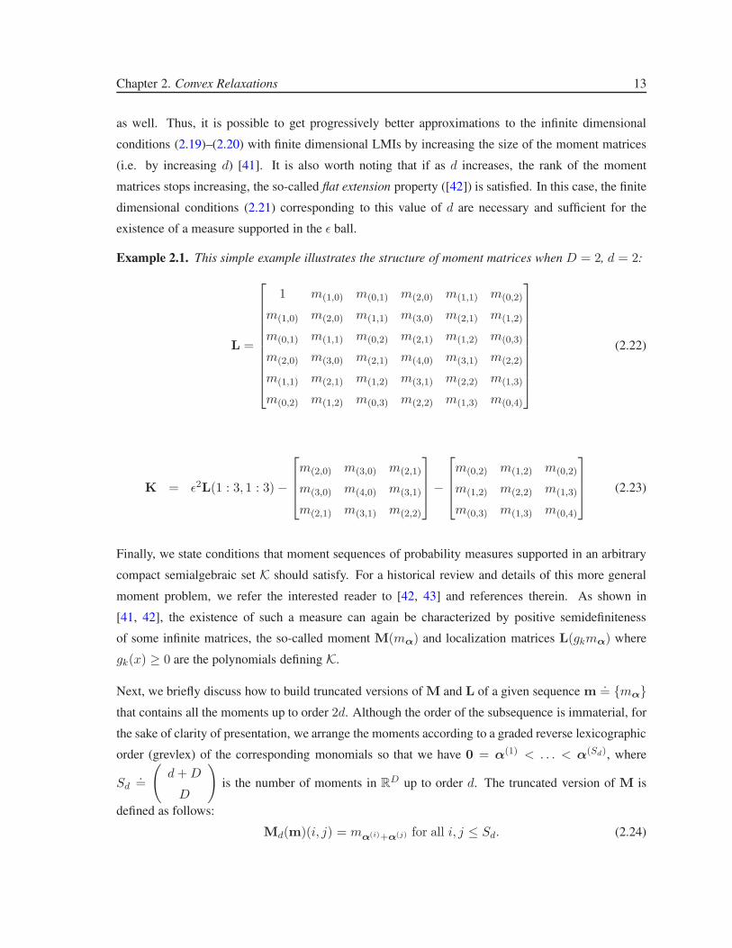
Example 2.1. This simple example illustrates the structure of moment matrices when D = 2, d = 2:
L =
1 m(1,0) m(0,1) m(2,0) m(1,1) m(0,2)
m(1,0) m(2,0) m(1,1) m(3,0) m(2,1) m(1,2)
m(0,1) m(1,1) m(0,2) m(2,1) m(1,2) m(0,3)
m(2,0) m(3,0) m(2,1) m(4,0) m(3,1) m(2,2)
m(1,1) m(2,1) m(1,2) m(3,1) m(2,2) m(1,3)
m(0,2) m(1,2) m(0,3) m(2,2) m(1,3) m(0,4)
(2.22)
K = ǫ2L(1 : 3, 1 : 3) −
m(2,0) m(3,0) m(2,1)
m(3,0) m(4,0) m(3,1)
m(2,1) m(3,1) m(2,2)
−
m(0,2) m(1,2) m(0,2)
m(1,2) m(2,2) m(1,3)
m(0,3) m(1,3) m(0,4)
(2.23)
Finally, we state conditions that moment sequences of probability measures supported in an arbitrary
compact semialgebraic set K should satisfy. For a historical review and details of this more general
moment problem, we refer the interested reader to [42, 43] and references therein. As shown in
[41, 42], the existence of such a measure can again be characterized by positive semidefiniteness
of some infinite matrices, the so-called moment M(mα) and localization matrices L(gkmα) where
gk(x) ≥ 0 are the polynomials defining K.
Next, we briefly discuss how to build truncated versions of M and L of a given sequence m.= {mα}
that contains all the moments up to order 2d. Although the order of the subsequence is immaterial, for
the sake of clarity of presentation, we arrange the moments according to a graded reverse lexicographic
order (grevlex) of the corresponding monomials so that we have 0 = α(1) < . . . < α(Sd), where
Sd.=
(
d + D
D
)
is the number of moments in RD up to order d. The truncated version of M is
defined as follows:
Md(m)(i, j) = mα(i)+α(j) for all i, j ≤ Sd. (2.24)

Chapter 2. Convex Relaxations 14
Let gk(x) =∑
β gk,β(l)xβ(l)be one of the defining polynomials of K with coefficients gk,β(l) and
degree δk, then the corresponding truncated localization matrix is defined as:
Ld(gkm)(i, j) =∑
β gk,β(l)mβ(l)+α(i)+α(j)
for all i, j ≤ Sd−⌊
δk2
⌋
(2.25)
2.2.2 Polynomial Optimization via Moments
This section reviews some results from [41] that relate polynomial optimization to the problem of
moments. Specifically, consider the problem of minimizing a real valued polynomial:
p∗K := minx∈K
p(x) (P1)
where K ⊂ RD is a compact set defined by polynomial inequalities. This problem is usually non-
convex, hence hard to solve. Next, we consider a related problem:
p∗K := minµ∈P(K)
∫
p(x)µ(dx) := minµ∈P(K)
Eµ [p(x)] (P2)
where P(K) is the space of finite Borel signed measures on K. Although (P2) is an infinite dimensional
problem, it is, in contrast to (P1), convex. The next result, taken from [41], establishes the relation
between the two problems:
Theorem 3. Problems (P1) and (P2) are equivalent; that is:
• p∗K = p∗K.
• If x∗ is a global minimizer of (P1), then µ∗ = δx∗ (the Dirac at x∗) is a global minimizer of
(P2).
• For every optimal solution µ∗ of (P2), p(x) = p∗, µ∗ almost everywhere.
Proof. See Proposition 2.1 in [41].
One direct consequence of this theorem is that when combined with the LMI-based characterizations
of moments presented in Section 2.2.1, it is possible to convert the infinite dimensional problem (P2) in
measures (or equivalently, the polynomial optimization problem (P1)) to a semidefinite programming
Chapter 2. Convex Relaxations 15
problem in the moments. When probability measures are supported on compact intervals (i.e. one
dimensional case), (P2) can be reduced to a finite dimensional LMI optimization problem in the mo-
ments. In the more general multidimensional case, it is possible to obtain asymptotically convergent
SDP relaxations. To this effect, define
p∗d = minm
∑
α pαmα
s.t.
Md(m) � 0,
Ld(gkm) � 0, k = 1, . . . , ng
(2.26)
where moment Md(m) and localization Ld(gkm) matrices are as defined in equations (2.24) and
(2.25).
Theorem 4. As d → ∞, p∗d ↑ p∗K.
Proof. See [41].
2.2.2.1 Exploiting the Sparse Structure
The next property will play a key role in reducing the computational complexity of problem (P1) by
exploiting its structure.
Definition 1. Let K ∈ RD be a semialgebraic set defined by ng polynomials gk. Let Ik ⊂ {1, . . . ,D}
be the set of indices of variables such that each gk contains variables from some Ik and assume that
the objective function p can be partitioned as p = p1 + . . . + pl where each pj contains only variables
from some Ik. If there exists a reordering Ik′ of Ik such that for every k′ = 1, . . . , d − 1:
Ik′+1 ∩k′
⋃
j=1
Ij ⊆ Is for some s ≤ k′ (2.27)
then the running intersection property is satisfied.
For the case of generic polynomials and constraints, solving problem (P1) using the method of mo-
ments requires considering moments and localization matrices containing O(D2d) variables. On the
other hand, if the running intersection property holds, it can be shown [44, 45] that it is possible to
define ng sets of smaller sized matrices each containing only variables in Ik (i.e. number of vari-
ables is O(κ2d), where κ is the number of elements in the maximum cardinality set among Ik’s). In

Chapter 2. Convex Relaxations 16
many practical applications, including the one considered in Chapter 4, κ ≪ n. Hence, exploiting
the sparse structure substantially reduces the number of variables in the optimization (and hence the
computational complexity), while still providing convergent relaxations.

Chapter 3
Identification of a Class of Hybrid
Dynamical Systems
3.1 Introduction and Motivation
Hybrid systems, systems characterized by the interaction of both continuous and discrete dynamics,
have been the subject of considerable attention during the past decade. These systems arise naturally
in many different contexts, e.g. biological systems, systems incorporating logical and continuous el-
ements, manufacturing, etc, and in addition, can be used to approximate nonlinear dynamics. As a
result of this research, an extensive body of results is now available addressing issues such as control-
lability/observability, stability analysis and control synthesis. However, applying these results requires
using an explicit model of the system under consideration. While in some cases these models can be
obtained from first principles, many practical applications require identifying the system from a com-
bination of experimental data and some a priori information. This has prompted a substantial research
effort devoted towards developing a framework for input/output identification of hybrid systems. As a
result, several methods have been proposed addressing different aspects of the problem (see the excel-
lent tutorial paper [46] for a summary of the main issues and recent developments in the field). While
successful in many situations, a common feature of these methods is the computational complexity
entailed in dealing with noisy measurements: in this case algebraic procedures [47] lead to noncon-
vex optimization problems, while optimization methods lead to generically NP–hard problems, either
necessitating the use of relaxations [48] or restricted to small size problems [49].
17
Chapter 3. Identification of a Class of Hybrid Dynamical Systems 18
Motivated by the computational complexity noted above, in the first portion of this dissertation we pro-
pose a new framework to the problem of set membership identification of a class of hybrid systems:
switched affine models. Specifically, given noisy input/output data and some minimal a priori infor-
mation about the set of admissible plants, our goal is to identify a suitable set of affine models along
with a switching sequence that can explain the available experimental information, while optimizing a
performance criteria (either minimum number of plants or minimum number of switches). Our main
result shows that this problem can be reduced to a sparsification form, where the goal is to minimize
the number of non–zero elements of a given vector sequence. Although in principle this leads to an
NP-hard problem, efficient convex relaxations can be obtained by exploiting recent results on sparse
signal recovery based on ℓ1-norm minimization [20, 21]. Then, we illustrate these results using two
non-trivial problems arising in computer vision applications: segmentation of video sequences and
of dynamic textures. As shown there, application of the proposed techniques outperforms existing
state-of-the-art techniques.
In the second part, we consider the hybrid system identification problem when the number of subsys-
tems is known. In this case we propose a moments-based convex optimization approach. The starting
point is the algebraic geometric procedure due to Vidal et al. [47, 50]. In the case of noiseless mea-
surements, the (unknown) parameters of each subsystem are recovered from the null space of a matrix
V(r) constructed from the input/output data r via a nonlinear embedding (the Veronese map). In the
case of noisy data, the entries of this matrix depend polynomially on the unknown noise terms. Thus,
finding a model in the consistency set (e.g. a model that interpolates the data within the unknown noise
level) is equivalent to finding an admissible noise sequence η that renders the matrix V(r) is rank de-
ficient, and a vector c in its null space. However, this is not a trivial problem, given the polynomial
dependence noted above. The main result of this section shows that the problem of jointly finding η
and c is equivalent to minimizing the rank of a matrix whose entries are affine in the optimization vari-
ables, subject to a convex constraint imposing that these variables are the moments of an (unknown)
probability distribution function with finite support. This results is achieved by using first an idea
similar to that of [41] relating polynomial optimization and the problem of moments, to eliminate the
polynomial dependence on the optimization variables, albeit at the price of introducing infinitely many
constraints. The structure of the problem, and in particular the independence of the noise terms, can
then be exploited to decouple this problem into several finite dimensional smaller ones, each involving
only the moments of a one–dimensional distribution. Combining these ideas with a convex relaxation,
similar to log-det heuristic of [51], that aims at dropping the rank of V by one and estimating a vector
in its nullspace, allows for recasting the original problem into a semidefinite optimization form that
Chapter 3. Identification of a Class of Hybrid Dynamical Systems 19
can be solved efficiently. We illustrate the performance of the proposed method with one academic
and one practical example.
3.2 Definitions
In this section we will consider switched autoregressive exogenous (SARX) hybrid affine models of
the form:
y(t) =
na∑
i=1
ai(σt)y(t − i) +
nc∑
i=1
ci(σt)u(t − i) + f(σt) + η(t) (3.1)
where u, y and η denote the input, output and noise, respectively, and where t ∈ [to, T ]. The discrete
variable σt ∈ {1, . . . , s}–the mode of the system– indicates which of the s submodels is active at time
t. The time instants where the value of σt changes are called discrete transitions or switches. These
switches partition the interval [t0, T ] into a discrete hybrid time set [52], τ = {Ii}ki=0, such that σt is
constant within each subinterval Ii = [τi, τ′i ] and different in consecutive intervals. In the sequel we
denote by τi and τ ′i the beginning and ending times of the ith interval, respectively. Clearly, τ satisfies:
• τ0 = t01 and τ ′
k = T ,
• τi ≤ τ ′i = τi+1 − 1,
and the number of switches is equal to k.
An equivalent representation of (3.1) is:
y(t) = p(σt)T r(t) + η(t) (3.2)
where r(t) = [y(t−1), . . . , y(t−na), u(t−1), . . . , u(t−nc), 1]T is the regressor vector and p(σt) =
[a1(σt), . . . , ana(σt), c1(σt), . . . , cnc(σt), f(σt)]T is the unknown coefficient vector at time t.
1Since it is not possible to deduce information for t < max(na, nc) when the initial conditions are unknown, in the
identification problem we take t0 = max(na, nc).
Chapter 3. Identification of a Class of Hybrid Dynamical Systems 20
3.3 Problem Statement
In this section we consider the problem of identifying switched autoregressive exogenous (SARX)
hybrid affine models from experimental measurements corrupted by noise. From a set-membership
point of view, this problem can be formally stated as follows:
Problem 1. [Consistency] Given input/output data over the interval [t0, T ], and a bound ǫ on the ℓp
norm of the noise (i.e. ‖η‖ ≤ ǫ), find a hybrid affine model of the form (3.1) that is consistent with the
a priori information and experimental data.
It is clear that this problem, though ensuring consistency, is not well-posed and has infinitely many
solutions. For instance, one can always find a trivial hybrid model with T − t0 + 1 submodels or one
model with a large order that perfectly fits the data. This situation can be partially avoided by imposing
upper bounds ny and nu on the order of each of the terms on the right hand side of (3.1), e.g. na ≤ ny
and nc ≤ nu for some known ny, nu. Still, even in this case the problem admits multiple solutions.
More interesting problems can be posed by using the existing degrees of freedom to optimize suitable
performance criteria.
One such criterion is to minimize the number of switches (i.e. minimum k), subject to consistency.
Practical situations where this problem is relevant arise for instance in segmentation problems in com-
puter vision and medical image processing, where it is desired to maximize the size of regions (roughly
equivalent to minimizing the number of boundaries), and in fault-detection, in cases where it is desired
to minimize the number of false alarms.2 This criterion may also be useful when the piecewise con-
stant mode signal σt is known to satisfy a dwell-time constraint (i.e. the time between any consecutive
switches is bounded below by a dwell-time) or an average dwell-time constraint (i.e. the number of
switches in any given interval is bounded above by its length normalized by an average dwell-time,
plus a chatter bound)3. The formal statement of the identification problem with this criterion is as
follows:
Problem 2. [Minimum Number of Switches] Given input/output data over the interval [t0, T ], and
bounds ǫ > ‖η‖p, nu ≥ nc and ny ≥ na on the ℓp norm of the noise and the order of the regressors,
respectively, find a hybrid affine model of the form (3.1) that is consistent with the a priori information
and that can explain the experimental data with the minimum number of switches.
2A similar problem is considered in econometrics society [53] where a dynamic programming approach is developed for
a fixed number of switches (i.e. when k is known).3These are the discrete-time counterparts of some sets of mode signals defined in [54]. Detailed definitions of different
sets of mode signals can be found therein.

Chapter 3. Identification of a Class of Hybrid Dynamical Systems 21
An alternative is to try to find the minimum number of submodels (i.e. minimum s) capable of ex-
plaining the data record. This criterion, used in [48], leads to the following identification problem:
Problem 3. [Minimum Number of Submodels] Given input/output data over the interval [t0, T ], and
bounds ǫ, ny, nu on the norm of the noise and regressor orders, find a hybrid affine model of the
form (3.1) with minimum number of submodels that is consistent with the a priori information and
experimental data.
3.4 A Sparsification Approach
In this section, we develop identification schemes where we pose an optimization problem that is in
the form of a sparse signal recovery problem. In Section 2.1, we present some background results on
sparsification and their extensions that will be used to recast the identification problem into a convex
optimization form.
3.4.1 Main Results
In this section we show that both, Problems 2 and 3, can be converted into an equivalent sparsification
form where the objective is to maximize the number of zero elements of a suitably defined vector
valued sequence. While in principle maximizing sparsity is a generically non-convex, hard to solve
problem, recent developments in sparse signal recovery reveal that efficient, computationally tractable
relaxations can be obtained by exploiting elements from convex analysis. To this effect, we start by
defining a time varying parameter vector p(t) ∈ Rny+nu+1. Replacing p(σt) in (3.2) with p(t),
allows for recasting the consistency problem into the following feasibility form:
find p(t)
s.t y(t) − r(t)Tp(t) = η(t) ∀t
‖{η}‖∗ ≤ ǫ
(3.3)
where ‖.‖∗ denotes a suitable norm, specified according to the problem under consideration, and where
ǫ is an upper bound on the noise level. Thus, restricting problems 2 and 3 to the feasible set of (3.3)
guarantees consistency.
Chapter 3. Identification of a Class of Hybrid Dynamical Systems 22
3.4.1.1 Identification with Minimum Number of Switches
In this section we address Problem 2 and show that in the case of ℓ∞ bounded noise, it can be reduced
to a convex optimization. For general convex noise descriptions, the problem can be converted into
an equivalent sparsification form where the objective is to maximize the number of zero elements of a
suitably defined vector valued sequence. The resulting (non–convex) optimization can then be solved
using the relaxation proposed in Lemma 1 in the Appendix.
A Greedy Algorithm for the ℓ∞ Case: In the sequel we propose a computationally simple algo-
rithm for solving Problem 2 in the case where the noise term is characterized in terms of its ℓ∞ norm.
This solution is motivated by existing results in time series clustering showing that a greedy sliding
window algorithm [55] is optimal. As we show below, similar ideas can be applied to problem 2,
leading to an algorithm that entails solving a sequence of smaller linear programs in a greedy fashion.
Greedy Algorithm
k = 0
t0 = max(ny, nu)
τk = t0
FOR i = t0 : T
Solve the following feasibility problem in p:
F :{
∣
∣y(t) − r(t)T p∣
∣ ≤ ǫ ∀t ∈ [τk, i]}
IF F is infeasible
Set Ik = [τk, i − 1], k = k + 1, and τk = i
END IF
END FOR
Set Ik = [τk, T ] and τ = {Ij}kj=0
RETURN τ and k
TABLE 3.1: Optimal Greedy Algorithm for Problem 2
Theorem 5. Let k∗ denote the number of switches in an optimal solution to Problem 2 when the noise
is characterized in terms of an ℓ∞ bound: ‖{η}‖∞ ≤ ǫ. Then the value k returned by the greedy
algorithm outlined in Table 3.1 coincides with the optimal k∗.

Chapter 3. Identification of a Class of Hybrid Dynamical Systems 23
Proof. Assume τ∗ = {I ∗i }k∗
i=0 is the discrete hybrid time set corresponding to an optimal solution with
k∗ switches. Let τ = {Ii}ki=0 and k be the pair of values returned by the greedy algorithm. In order
to establish that the proposition is true, it is enough to show that if τi ∈ I∗j then τ ′
i ≥ τ ′j∗. Then, an
induction step shows that, τ ′i ≥ τ ′
i∗ ∀i ∈ {0, . . . , k∗} implying k ≤ k∗.
Since τ∗ is optimal (hence feasible), p∗(t) is constant in each subinterval I∗. In particular, there
exists pj such that for all t ∈ I∗j , p∗(t) = pj and
∣
∣y(t) − r(t)T pj
∣
∣ ≤ ǫ. When τi ∈ I∗j , the same
pj is a feasible solution of F in the (τ ′j∗)th iteration of the greedy algorithm since τi ∈ I
∗j implies
[τi, τ′j∗] ⊆ I
∗j . Therefore, the algorithm will continue to the next iteration without entering the if
condition within the for loop, which implies τ ′i ≥ τ ′
j∗.
Next, we show by induction that for all i ≤ k, there exists j ≥ i such that τ ′i ≥ τ ′
j∗, hence τ ′
i ≥ τ ′i∗:
• For i = 0: τ0 = τ∗0 ∈ I
∗0 ⇒ τ ′
0 ≥ τ ′0∗.
• For i = m: Assume ∃j ≥ m s.t. τ ′m ≥ τ ′
j∗.
• For i = m + 1: From the previous line and properties of hybrid time sets, we have that τm+1 =
τ ′m + 1 > τ ′
m ≥ τ ′j∗ ⇒ ∃l > j (or equivalently ∃l ≥ j + 1) s.t. τm+1 ∈ I
∗l ⇒ τ ′
m+1 ≥ τ ′l∗ ≥
τ ′j+1
∗. Since j ≥ m implies j + 1 ≥ m + 1, this proves the induction hypothesis.
Using the fact that T = τ ′k = τ ′
k∗
∗and the result of the induction particularly at i = k leads to
τ ′k ≥ τ ′
k∗ ⇒ τ ′
k∗
∗ ≥ τ ′k∗ ⇒ k∗ ≥ k.
Since by construction the result of the greedy algorithm is feasible for problem 2 and k∗ is the mini-
mum solution of the problem, k∗ ≤ k. Therefore, k∗ = k.
Remark 3. By construction, the greedy algorithm pushes the end points of each interval forward in
time as much as possible (i.e. τ ′i is as large as possible). Similarly, running the algorithm backwards
(i.e. i = T : t0) would push the start points of intervals (equivalently, end points of previous intervals)
backward in time as much as possible. Therefore, running it once backwards and once forwards, it is
possible to bracket the true locations of the switches.
Identifiability of the Switches and Convergence of the Greedy Algorithm: In this section, we
address the issue of identifiability of the switches from input output data. We first present a necessary
and sufficient condition under which the switches can be exactly identified in a noiseless setup. Later,
Chapter 3. Identification of a Class of Hybrid Dynamical Systems 24
we show that when these identifiability conditions hold, the greedy algorithm given in Table 3.1 finds
the exact switching times for sufficiently small noise levels (i.e., as ǫ → 0).
Definition 2. Let τ = {Ii}ki=0 be a hybrid time set corresponding to a particular trajectory of a switched
linear ARX system. τ is said to be causally identifiable if whenever σt−1 6= σt, it is possible to detect
the switch as soon as y(t) is observed.
Definition 3. Given the current regressor vector r(t), two submodels with parameter vectors p1 and
p2 are one-step indistinguishable from r(t) if r(t)T (p1 − p2) = 0.
The next result presents a necessary and sufficient condition for a switching sequence to be causally
identifiable from input output data. Here, for notational simplicity, we define Rt0,t1 = [r(t0), r(t0 +
1), . . . , r(t1)], Yt0,t1 = [y(t0), y(t0 + 1), . . . , y(t1)]T and Nt0,t1 = [η(t0), η(t0 + 1), . . . , η(t1)]
T .
Lemma 3. If r(τi+1) ∈ range(
Rτi,τ ′
i
)
then rT (τi+1) [pi+1 − pi] = constant for all pairs (pi,pi+1)
satisfying
Yτi,τ ′
i= RT
τi,τ ′
ipi
y(τi+1) = rT (τi+1)pi+1
(3.4)
Proof. Since r(τi+1) ∈ range(
Rτi,τ ′
i
)
then rT (τi+1) = vTRTτi,τ ′
ifor some v 6= 0. Consider now
two pairs (pi,pi+1) and (pi, pi+1) satisfying (3.4). Then
rT (τi+1) [pi+1 − pi] − rT (τi+1) [pi+1 − pi] = rT (τi+1) [pi − pi]
= vT[
RTτi,τ ′
ipi − RT
τi,τ ′
ipi
]
= 0
where the last equality follows from the first equality in (3.4).
Theorem 6. In the noise free case, τ = {Ii}ki=0 is causally identifiable from input/output data if and
only if the following two conditions hold for all i:
rT (τi+1) [pi+1 − pi] 6= 0 (3.5)
r(τi+1) ∈ range(
Rτi,τ ′
i
)
(3.6)
Proof. Necessity: Clearly (3.5) is necessary for the switch to be detectable. To show that (3.6) is also
necessary, assume that it fails. Then rT (τi+1)R⊥τi,τ ′
i
.= vT 6= 0, where R⊥
τi,τ ′
idenotes a basis for the
orthogonal complement of Rτi,τ ′
i. Define:
p.= pi +
y(τi+1) − rT (τi+1)pi
‖v‖2R⊥
τi,τ ′
iv
Chapter 3. Identification of a Class of Hybrid Dynamical Systems 25
Simple algebra shows that p satisfies Yτi,τ ′
i= RT
τi,τ ′
ip and y(τi+1) = rT (τi+1)p. It follows that the
model
y(t) = rT (t)p (3.7)
can explain all the data in the interval [τi, τi+1], and thus the switch is not causally detectable from the
input/output data alone.
Sufficiency: Since rT (τi+1) [pi+1 − pi] 6= 0, it follows, from Lemma 3, that there does not exist a
single p such that (3.7) holds for all t ∈ [τi, τi+1]. Hence the switch is causally detectable from the
input/output sequences {u, y}.
Remark 4. The results about formalizes the intuition that a switch is causally detectable if and only
in the two modes involved are not one–step indistinguishable and no new modes of the present model
have been excited at the last time step (condition (3.6)). In addition, it can be shown that conditions
(3.5)–(3.6) are equivalent to
rank[Yτi,τi+1 RTτi,τi+1
] > rank[RTτi,τi+1
] (3.8)
However, the former are easier to generalize to the noisy case.
The next result shows that if the identifiability conditions (3.5)–(3.6) hold, the greedy algorithm finds
the exact switches for sufficiently small noise levels.
Theorem 7. If a hybrid time set τ is causally identifiable, then there exists a noise level ǫ0 such that
greedy algorithm finds the switches correctly whenever the noise level ǫ is below ǫ0.
Proof. In order to show that the greedy algorithm correctly identifies the hybrid time set τ , we need
to show that
∥
∥y(τi+1) − r(τi+1)T p∥
∥ > ǫ (3.9)
for all p such that
RTτi,τ ′
ip = Yτi,τ ′
i+ Nτi,τ ′
i(3.10)
or, equivalently∥
∥r(τi+1)T pi+1 − r(τi+1)
Tp∥
∥ ≥ 2ǫ for all p that satisfy (3.10). Since τ is identifiable
by hypothesis, it follows from Theorem 6 that for i ∈ {I}, r(τi+1) ∈ range(
Rτi,τ ′
i
)
. Hence,
r(τi+1) = Rτi,τ ′
iλ for some λ 6= 04 and ‖r(τi+1)‖2 ≥ σRi
‖λ‖2, where σRidenotes the smallest
4If Rτi,τ ′
idoes not have full column rank, this representation is not unique. In this case, we choose λ∗ with minimum
2-norm.
Chapter 3. Identification of a Class of Hybrid Dynamical Systems 26
(non–zero) singular value of Rτi,τ ′
i. It follows that, for all (p, p that satisfy (3.10) we have
r(τi+1)T (p− p) = λTRT
τi,τ ′
i(p− p) = λT
(
Nτi,τ ′
i− Nτi,τ ′
i
)
Hence
∣
∣r(τi+1)T (p− p)
∣
∣ ≤ ‖λ‖2
√
(τi − τi+1)2ǫ ≤ 2‖r(τi+1)‖2
√
(τi − τi+1)
σR
ǫ.= b(ǫ) (3.11)
In addition, identifiability of τ implies that
∥
∥r(τi+1)Tpi+1 − r(τi+1)
T pi
∥
∥ = γi > 0 (3.12)
From (3.11) and (3.12), it follows that, if the noise level ǫ satisfies
ǫ < mini∈{I}
σRiγi
2(
‖r(τi+1)‖2
√
(τi − τi+1) + σRi
) (3.13)
then (3.9) holds for all i ∈ {I} and hence all switches will be correctly detected by the greedy
algorithm.
The Case of General Convex Noise Descriptions: In the case of general noise descriptions η ∈ N
all samples are coupled through the noise description. This requires the use of batch algorithms that
consider all available data, as opposed to the greedy one used in the ℓ∞ case. As we show next,
in this case the problem can be reduced to a sparsification form and efficiently reduced to a convex
optimization using the tools described in the Appendix. The starting point it to consider the sequence
of first order differences of the time varying parameters p(t), given by
g(t) = p(t) − p(t + 1) (3.14)
Clearly, since a non-zero element of this sequence corresponds to a switch, the sequence should be
sparse having only k non-zero elements out of T − t0. Thus, with this definition, Problem 2 is equiv-
alent to the following (non–convex) sparsification problem:
Chapter 3. Identification of a Class of Hybrid Dynamical Systems 27
minp(t) ‖{p(t) − p(t − 1)}‖0
s.t y(t) − r(t)T p(t) ∈ N ∀t(3.15)
From Lemma 1 in the Appendix, it follows that a convex relaxation can be obtained replacing ‖.‖o
by ‖.‖1. A better heuristic can be obtained by adapting to this case the iterative weighted ℓ1 heuristic
proposed in ([51, 56, 57]). This requires solving, at each iteration, the following convex program:
minimizez,p∑
t w(k)t zt
subject to ‖p(t) − p(t − 1)‖∞ ≤ zt ∀t
y(t) − r(t)Tp(t) ∈ N ∀t
(3.16)
where w(k)t = (z
(k)t + δ)−1 and where z
(k)t denotes the optimal solution at the kth iteration, with
z(0) = [1, 1, . . . , 1]T , and δ is a (small) regularization constant.
In the first iteration, this method solves the standard ℓ1-norm relaxation. Then at each subsequent
iteration, it increases the weight w(k)t associated with the small z
(k)t s, thus pushing these elements
further towards zero.
Remark 5. Algorithm (3.16) requires solving m linear programs with (ny + nu + 2) × (T − t0 + 1)
variables and 2(ny +nu +2)×(T − t0 +1) inequality constraints, where m is the number of iterations
required for convergence of the weighted ℓ1-norm relaxation, typically around 5. On the other hand,
the greedy algorithm requires solving (T − t0 + 1) linear programs with only (ny + nu + 1) variables
and at most 2(T − t0 + 1) inequality constraints (the worst case scenario is when a single parameter
value is feasible for the entire [t0, T ] interval). Thus, in cases where both algorithms are applicable
(e.g. when the noise is characterized in terms of its ℓ∞ norm), the greedy algorithm is preferable from
a computational complexity standpoint.
Extension to Multi-input Multi-output Models: It is straight forward to extend the sparsity based
identification procedure with minimum number of switches criterion to multi–input multi–output
(MIMO) models. Consider the MIMO switched ARX model with mu inputs and my outputs:
y(t) =
na∑
i=1
Ai(σt)y(t − i) +
nc∑
i=1
Ci(σt)u(t − i) + f(σt) + η(t) (3.17)
where y ∈ Rmy , u ∈ R
mu are outputs and inputs, Ai ∈ Rmy×my , Ci ∈ R
my×mu and f ∈ Rmy
are coefficient matrices, and η ∈ Rmy is the noise, respectively. It is possible to solve for coefficient

Chapter 3. Identification of a Class of Hybrid Dynamical Systems 28
matrices in a similar manner as in (3.16). Particularly, the following modification steps are required: (i)
define time varying coefficient matrices (i.e. Ai(t), Ci(t) and f(t)) (ii) form p(t) ∈ Rm2
y+mymu+my
by stacking the elements of the coefficient matrices at time t into a column vector, and (iii) replace the
regressor equation in (3.16) with the multivariate regressor corresponding to (3.17).
Extension to Multidimensional Models: In this section we consider the identification of hybrid
multidimensional systems (i.e. hybrid systems where the process dynamics depend on more than
one indeterminate). In particular, systems that are governed by affine switched-coefficient difference
equations (ASCDEs) are considered. ASCDE is a generalization of the so-called linear constant-
coefficient difference equations (LCCDEs) ([58]). An n-dimensional ASCDE has the following form:
y(t1, . . . , tn) =∑
(k1,...,kn)∈Raak1,...,kn
(σt1,...,tn)y(t1 − k1, . . . , tn − kn)
+∑
(k1,...,kn)∈Rcck1,...,kn
(σt1,...,tn)u(t1 − k1, . . . , tn − kn)
+f(σt1,...,tn) + η(t1, . . . , tn)
(3.18)
where y is the output; u is the input; η is noise; σt1,...,tn ∈ {1, . . . , s} is the discrete mode signal as
before. Ra,Rc ⊂ Zn are coefficient support regions; and ak1,...,kn
(σt1,...,tn), ck1,...,kn(σt1,...,tn) and
fk1,...,kn(σt1,...,tn) are the coefficients to be identified.
3-D models of this form in noise-free setup are considered in [59] for spatiotemporal segmentation.
Such a model can be useful in approximating the behavior of a wave traveling in an inhomogeneous
space or the images where different regions of the image are occupied by different textures.
As a shorthand notation, we denote the indeterminate in vector form, i.e. t = [t1, . . . , tn] ∈ Zn. Let
D ⊂ Zn denote the domain over which experimental measurements are collected. The interior of the
domain can be prescribed as:
int(D) = {t ∈ D| t − k ∈ D ∀k ∈ Ra ∀k ∈ Rc} (3.19)
Now, we can define the set of neighboring indices as a set of unordered pairs:
I ={{
t, t}
|∥
∥t − t∥
∥
1= 1, and t, t ∈ int(D)
}
. (3.20)
A switch is defined between neighboring indices. That is, we say that there is a switch whenever
σt 6= σt for{
t, t}
∈ I (analogous to 1D case where switches are defined between t and t + 1). A
Chapter 3. Identification of a Class of Hybrid Dynamical Systems 29
multidimensional hybrid “time” set is a partition {Pi} of int(D) such that within each part (where we
call the elements of partition as parts or segments) σt is constant and it is different between neighboring
parts (Pi and Pj are called neighboring parts if there exists{
t, t}
∈ I such that t ∈ Pi and t ∈ Pj).
As in the 1D case, identification of a system of the form (3.18) is ill-posed since for example one can
choose a partition where each part consists of a single t. We are interested in finding a partition with
minimum number of switches (this corresponds to minimizing the boundary of the segments in image
segmentation problem). In order to minimize the number of switches, one should consider sparsifying
the following difference sequence:
g(i) = p(t) − p(t),{
t, t}
∈ I (3.21)
where p(t) = [ak1(σt), . . . , akna(σt), ck1(σt), . . . , cknc
(σt), f(σt)], and i = 1, . . . , |I| is an index
counting the elements of I . Then, the identification problem can be written as:
minp(t) ‖{g(i)}‖0
s.t Equation (3.18)
‖{η}‖∗ ≤ ǫ
(3.22)
which can be solved, exactly as in the 1D case, with the weighted ℓ1 norm approximation.
3.4.1.2 Identification with Minimum Number of Submodels:
In this section, motivated by an idea used in [48], we present an iterative procedure for solving Problem
3. The main idea is to find one submodel at a time, along with the associated parameter vector p,
through the solution of a sparsification problem. This is accomplished by finding a parameter vector p
that makes∣
∣y(t) − r(t)T p∣
∣ ≤ ǫ feasible for as many time instants t as possible. Equivalently, defining
g(t) = p(t) − p, the goal is to maximize sparsity of g(t) leading to the following optimization
problem:
minp(t),p ‖{p(t) − p}‖0
s.t∣
∣y(t) − r(t)T p(t)∣
∣ ≤ ǫ ∀t(3.23)

Chapter 3. Identification of a Class of Hybrid Dynamical Systems 30
Algorithm for Minimum # of Submodels
t0 = max(ny, nu)
N1 = {t0, . . . , T}
l = 0
WHILE Nl+1 6= ∅
Let l = l + 1
Find pl by solving the re–weighted ℓ1 optimization:
minzt,p(t),p
∑
t w(k)t zt
subject to ‖p(t) − p‖∞ ≤ zt ∀t ∈ Nl∣
∣y(t) − r(t)T p(t)∣
∣ ≤ ǫ ∀t ∈ Nl
where w(k)j = (z
(k)j + δ)−1 are weights with z
(k)j the arguments of the optimal solu-
tion in kth iteration and z(0) = [1, 1, . . . , 1]T ; and δ is the regularization constant.
Let i = 1
WHILE i < l
Let Kil ={
t ∈ Ni :∣
∣y(t) − r(t)T pl
∣
∣ ≤ ǫ}
IF #Kil > #Ki
Let pi = pl and l = i
END IF
Let i = i+1
END WHILE
Let Kl ={
t ∈ Nl :∣
∣y(t) − r(t)T pl
∣
∣ ≤ ǫ}
Let Nl+1 = Nl \ Kl
END WHILE
RETURN s = l and Ki, i = 1, . . . , s
TABLE 3.2: Algorithm for Problem 3
Then, we can eliminate the time instants t for which g(t) is zero, and solve the same problem with the
rest of the t’s up until all data points are clustered. The number of times (3.23) is solved gives an upper
bound on the minimum number of submodels s. Combining this idea with a refinement step similar to
the one proposed in [48] to re-estimate parameter values and reassign, if needed, data points, leads to
the overall algorithm listed in Table 3.2, where minimization of ‖.‖0 is (approximately) accomplished
through the use of the weighted ℓ1 norm minimization relaxation.
Next, we briefly discuss an alternative formulation of the problem (3.23). The main idea is similar
to that of above that is, to find a parameter vector p that makes[
y(t) − r(t)T p]
∈ N feasible for as

Chapter 3. Identification of a Class of Hybrid Dynamical Systems 31
many time instants t as possible. Equivalently, if we define e(t) = y(t)− r(t)T p+ η(t), the goal is to
maximize sparsity of e(t) leading to the following optimization problem:
mine(t),p ‖{e(t)}‖0
s.t[
e(t) − y(t) + r(t)T p]
∈ N ∀t(3.24)
We define, Rt0,T = [r(t0), r(t0+1), . . . , r(T )], y = [y(t0), y(t0+1), . . . , y(T )]T and e = [e(t0), e(t0+
1), . . . , e(T )]T . Assuming noise is characterized with a norm bound, we obtain the following sparsifi-
cation problem:
mine ‖e‖0
s.t
∥
∥
∥
∥
∥
[I Rt0,T ]
[
e
p
]
− y
∥
∥
∥
∥
∥
∗
≤ ǫ(3.25)
The advantage of this formulation over (3.23) is that instead of having a time dependent parameter
vector p(t), we just have the error sequence e(t) as unknowns. Hence, as long as number of outputs
ny is smaller than order of the regressor nc + na, there are less variables in optimization. The other
advantage is that problem (3.25) has the same form as standard sparse recovery problems for single
output systems.
Remark 6. While consistent numerical experience shows that the idea of finding one system at a time
works well in practice, counterexamples are available where it overestimates the number of systems.
This is due to its greedy nature that tends to assign as many points as possible to the parameters
found earlier, possibly resulting in the later need to use additional parameter values in order to explain
unassigned data points. At this point the issues of existence of conditions under which the greedy
algorithm is indeed optimal and bounds on its worst case performance are open research questions.
3.4.2 Examples
Example 1: This example illustrates the fact that dwell–time constraints are not necessary for identifi-
ability of the switches. Consider three autonomous systems (σt ∈ {1, 2, 3}) of the form:
yt = a1(σt)yt−1 + a2(σt)yt−2 + a3(σt)yt−3

Chapter 3. Identification of a Class of Hybrid Dynamical Systems 32
with
[a1(1), a2(1), a3(1)] = [−3, 2, 1]
[a1(2), a2(2), a3(2)] =[
13 , 1
3 , 13
]
[a1(3), a2(3), a3(3)] = [2,−1, 1]
and
σt =
1, t ∈ [1, 4]
2, t = 5
3, t = 6
The trajectory corresponding to the initial conditions y0 = 0, y−1 = 7, y−2 = −12, is given by
2, 1, 1, 1, 1, 2. Thus, the rank condition (3.8) evaluated at t = 6 yields
rank
[
1 1 1 1
2 1 1 1
]
= rank
[
1 1 1
1 1 1
]
+ 1
which implies that it is possible to detect the switch from t = 5 to t = 6 although the system remains
in σt = 2 for only one time instant.
Example 2: The goal of this example is to illustrate that noiseless switch identifiability does not imply
that mode switches are identifiable under arbitrarily small noise. To this effect consider a system with
2 submodels: the first corresponds to p1 =[
1/3 1/3 1/3]
, and is active for t=1,2. The second
corresponds to p2 =[
1 −1 2]
and is active for t=3. The trajectory corresponding to the initial
conditions r(1) =[
1 1 1]
and no external input is given by y(1) = 1, y(2) = 1 and y(3) = 2. In
this case the associated matrices satisfy:
rank
1 1 1 1
1 1 1 1
2 1 1 1
> rank
1 1 1
1 1 1
1 1 1
Hence the switch is causally identifiable. However, adding the noise sequence η(1) = ǫ, η(2) = 0,
η(3) = 0 leads to the trajectory: y(1) = 1 + ǫ, y(2) = 1 + ǫ3 , y(3)=2 − 2 ǫ
3 . In this case the
corresponding matrices satisfy:
rank
1 + ǫ 1 1 1
1 + ǫ3 1 + ǫ 1 1
2 − 2 ǫ3 1 + ǫ
3 1 + ǫ 1
= rank
1 1 1
1 + ǫ 1 1
1 + ǫ3 1 + ǫ 1
∀ǫ > 0
Chapter 3. Identification of a Class of Hybrid Dynamical Systems 33
Hence, the switch is not identifiable, regardless of how small ǫ is. This is due to the fact that in this
case condition (3.6) fails since r(3) =[
1 + ǫ3 1 + ǫ 1
]T6∈ range
[
1 1 1
1 + ǫ 1 1
]T
.
Example 3: In this example, we considered input/output data generated by a hybrid system that
switched among the following two ARX submodels:
y(t) = 0.2y(t − 1) + 0.24y(t − 2) + 2u(t − 1); t ∈ [1, 25] ∪ [51, 75]
y(t) = −1.4y(t − 1) − 0.53y(t − 2) + u(t − 1); t ∈ [26, 50] ∪ [76, 100]
with ‖η‖∞ = 0.5. The goal here was to identify a model that explained the experimental data record
with the fewest possible number of switches. Figure 3.1 compares the performance of sparsification-
based (both the ℓ1-based algorithm (3.15) and the greedy algorithm of Table 3.1) against the algebraic
method and the bounded error method. As shown there, the sparsification based methods correctly
estimated the parameters and number of switches, while the other two failed to do so. The running
times for ℓ1-based, greedy, algebraic and bounded error methods are 5.9, 40.5, 1.1 and 17.9 seconds
respectively. Additional examples illustrating the use of sparsification to find the minimum number of
switches are given in section 3.4.3.
For this example, ǫo in (3.13) was found to be 0.3136 which corresponds to 4.15% of the maximum
absolute value of the output y(t). Note that the analysis in section 3.4.1.1 is worst-case, meaning for
all noise values below ǫo = 0.3136, the greedy algorithm finds the correct switches. Even though the
noise level in our example was 0.5 which was above ǫo, greedy algorithm was still capable of correctly
detecting the switches.
Example 4: This example considers the problem of estimating the minimum number of systems and
investigates the effects of noise level on algorithm performance. The data used corresponded to the
trajectories of 100 randomly generated SARX models of the form:
y(t) = a1(σt)y(t − 1) + a2(σt)y(t − 2) + c1(σt)u(t − 1) + η(t) (3.26)
with
σt =
1, t ∈ [1, 60]
2, t ∈ [61, 120]
3, t ∈ [121, 180]
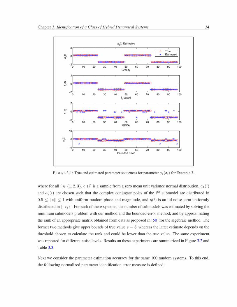
Chapter 3. Identification of a Class of Hybrid Dynamical Systems 34
0 10 20 30 40 50 60 70 80 90 100−2
0
2
a1(t) Estimates
a1(t
)
Greedy
True
Estimated
0 10 20 30 40 50 60 70 80 90 100−2
0
2
a1(t
)
l1 based
0 10 20 30 40 50 60 70 80 90 100−2
0
2
a1(t
)
GPCA
0 10 20 30 40 50 60 70 80 90 100−10
0
10
a1(t
)
Bounded Error
FIGURE 3.1: True and estimated parameter sequences for parameter a1(σt) for Example 3.
where for all i ∈ {1, 2, 3}, c1(i) is a sample from a zero mean unit variance normal distribution, a1(i)
and a2(i) are chosen such that the complex conjugate poles of the ith submodel are distributed in
0.5 ≤ ‖z‖ ≤ 1 with uniform random phase and magnitude, and η(t) is an iid noise term uniformly
distributed in [−ǫ, ǫ]. For each of these systems, the number of submodels was estimated by solving the
minimum submodels problem with our method and the bounded-error method; and by approximating
the rank of an appropriate matrix obtained from data as proposed in [50] for the algebraic method. The
former two methods give upper bounds of true value s = 3, whereas the latter estimate depends on the
threshold chosen to calculate the rank and could be lower than the true value. The same experiment
was repeated for different noise levels. Results on these experiments are summarized in Figure 3.2 and
Table 3.3.
Next we consider the parameter estimation accuracy for the same 100 random systems. To this end,
the following normalized parameter identification error measure is defined:
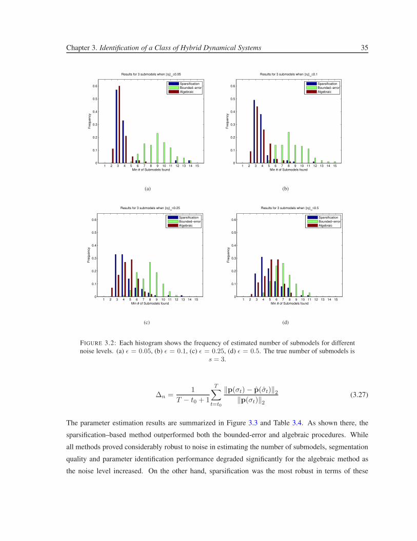
Chapter 3. Identification of a Class of Hybrid Dynamical Systems 35
1 2 3 4 5 6 7 8 9 10 11 12 13 14 150
0.1
0.2
0.3
0.4
0.5
0.6
Min # of Submodels found
Fre
qu
en
cy
Results for 3 submodels when ||η||∞
≤0.05
Sparsification
Bounded−error
Algebraic
(a)
1 2 3 4 5 6 7 8 9 10 11 12 13 14 150
0.1
0.2
0.3
0.4
0.5
0.6
Min # of Submodels found
Fre
qu
en
cy
Results for 3 submodels when ||η||∞
≤0.1
Sparsification
Bounded−error
Algebraic
(b)
1 2 3 4 5 6 7 8 9 10 11 12 13 14 150
0.1
0.2
0.3
0.4
0.5
0.6
Min # of Submodels found
Fre
qu
en
cy
Results for 3 submodels when ||η||∞
≤0.25
Sparsification
Bounded−error
Algebraic
(c)
1 2 3 4 5 6 7 8 9 10 11 12 13 14 150
0.1
0.2
0.3
0.4
0.5
0.6
Min # of Submodels found
Fre
qu
en
cy
Results for 3 submodels when ||η||∞
≤0.5
Sparsification
Bounded−error
Algebraic
(d)
FIGURE 3.2: Each histogram shows the frequency of estimated number of submodels for different
noise levels. (a) ǫ = 0.05, (b) ǫ = 0.1, (c) ǫ = 0.25, (d) ǫ = 0.5. The true number of submodels is
s = 3.
∆n =1
T − t0 + 1
T∑
t=t0
‖p(σt) − p(σt)‖2
‖p(σt)‖2
(3.27)
The parameter estimation results are summarized in Figure 3.3 and Table 3.4. As shown there, the
sparsification–based method outperformed both the bounded-error and algebraic procedures. While
all methods proved considerably robust to noise in estimating the number of submodels, segmentation
quality and parameter identification performance degraded significantly for the algebraic method as
the noise level increased. On the other hand, sparsification was the most robust in terms of these

Chapter 3. Identification of a Class of Hybrid Dynamical Systems 36
Noise Level ǫ Absolute Error Sparsification Bounded-Error Algebraic
0.05
Mean 1.40 (0.99) 6.20 0.52
Standard deviation 3.48 (2.66) 2.09 0.77
Median 0 (0) 6 0
Median absolute deviation 0 (0) 1 0
0.1
Mean 0.84 (1.04) 5.64 0.87
Standard deviation 1.36 (2.20) 2.03 1.02
Median 1 (0.5) 5 1
Median absolute deviation 1 (0.5) 1 1
0.25
Mean 1.59 (1.95) 4.84 1.60
Standard deviation 2.17 (2.31) 1.61 1.16
Median 1 (1) 5 1
Median absolute deviation 1 (1) 1 1
0.5
Mean 1.93 (2.39) 4.07 2.18
Standard deviation 1.65 (2.11) 1.58 1.25
Median 2 (2) 4 2
Median absolute deviation 1 (1) 1 1
TABLE 3.3: Minimum number of submodel estimation error statistics for different noise levels.
The results for sparsification is given both with formulation (3.23) and with formulation (3.24) in
parantheses.
performance criteria. The bounded-error method performed relatively poorly when estimating the
number of submodels. Even though it clustered most of the data in the largest three submodels, it also
generated superfluous submodels with parameter values far from the true values.
Among the two sparsification formulations (3.23) and (3.24) (results shown in parantheses in Tables
3.3 and 3.4 for the latter), we did not observe a significant difference in terms of these performance
criteria, with (3.23) performing slightly better. Also, although problem (3.24) involves less variables,
it required more iterations of the algorithm given in Table 3.2. Hence, the overall computation times
were also similar.
Example 5: For the next example, we present more numerical results on a single system. In particular,
we considered input/output data generated by an SARX system of the form (3.26) with the same mode
signal σt and coefficients:
[a1(1), a2(1), c1(1)] = [−1.6758, −0.8292, 1.8106]
[a1(2), a2(2), c1(2)] = [−0.8402, −0.6770, 0.2150]
[a1(3), a2(3), c1(3)] = [1.0854, −0.9501, 0.6941].
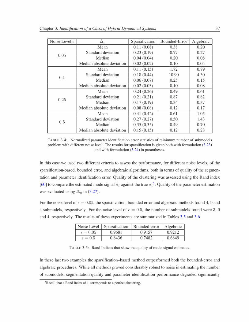
Chapter 3. Identification of a Class of Hybrid Dynamical Systems 37
Noise Level ǫ ∆n Sparsification Bounded-Error Algebraic
0.05
Mean 0.11 (0.08) 0.38 0.20
Standard deviation 0.23 (0.19) 0.77 0.27
Median 0.04 (0.04) 0.20 0.08
Median absolute deviation 0.02 (0.02) 0.10 0.05
0.1
Mean 0.11 (0.15) 1.72 0.79
Standard deviation 0.18 (0.44) 10.90 4.30
Median 0.06 (0.07) 0.25 0.15
Median absolute deviation 0.02 (0.03) 0.10 0.08
0.25
Mean 0.24 (0.26) 0.49 0.61
Standard deviation 0.21 (0.21) 0.87 0.82
Median 0.17 (0.19) 0.34 0.37
Median absolute deviation 0.08 (0.08) 0.12 0.17
0.5
Mean 0.41 (0.42) 0.61 1.05
Standard deviation 0.27 (0.27) 0.50 1.43
Median 0.35 (0.35) 0.49 0.70
Median absolute deviation 0.15 (0.15) 0.12 0.28
TABLE 3.4: Normalized parameter identification error statistics of minimum number of submodels
problem with different noise level. The results for sparsification is given both with formulation (3.23)
and with formulation (3.24) in parantheses.
In this case we used two different criteria to assess the performance, for different noise levels, of the
sparsification-based, bounded error, and algebraic algorithms, both in terms of quality of the segmen-
tation and parameter identification error. Quality of the clustering was assessed using the Rand index
[60] to compare the estimated mode signal σt against the true σt5. Quality of the parameter estimation
was evaluated using ∆n in (3.27).
For the noise level of ǫ = 0.05, the sparsification, bounded error and algebraic methods found 4, 9 and
4 submodels, respectively. For the noise level of ǫ = 0.5, the number of submodels found were 3, 9
and 4, respectively. The results of these experiments are summarized in Tables 3.5 and 3.6.
Noise Level Sparsification Bounded-error Algebraic
ǫ = 0.05 0.9681 0.9157 0.9212
ǫ = 0.5 0.8436 0.7482 0.6849
TABLE 3.5: Rand Indices that show the quality of mode signal estimates.
In these last two examples the sparsification–based method outperformed both the bounded-error and
algebraic procedures. While all methods proved considerably robust to noise in estimating the number
of submodels, segmentation quality and parameter identification performance degraded significantly
5Recall that a Rand index of 1 corresponds to a perfect clustering.
Chapter 3. Identification of a Class of Hybrid Dynamical Systems 38
0 0.1 0.2 0.3 0.4 0.50
0.2
0.4
0.6
0.8
1
Noise Level, ||η||∞
Para
mete
r E
stim
ation E
rror
Sparsification
Bounded error
Algebraic
FIGURE 3.3: Median of parameter estimation error ∆n versus noise level ǫ. Error bars indicate the
median absolute deviation.
Noise Level Sparsification Bounded-error Algebraic
ǫ = 0.05 0.0699 0.2883 0.0504
ǫ = 0.5 0.1459 0.8604 0.9245
TABLE 3.6: Error measure ∆n that shows the quality of parameter estimates.
for the algebraic method as the noise level increased. On the other hand, sparsification was the most
robust in terms of these performance criteria. The bounded-error method performed relatively poorly
when estimating the number of submodels. Even though it clustered most of the data in the largest
three submodels, it also generated superfluous submodels with parameter values far from the true
values.
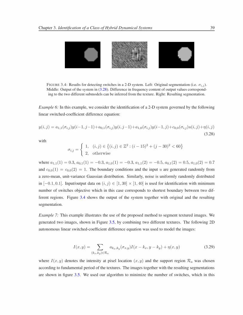
Chapter 3. Identification of a Class of Hybrid Dynamical Systems 39
FIGURE 3.4: Results for detecting switches in a 2-D system. Left: Original segmentation (i.e. σi,j ).
Middle: Output of the system in (3.28). Difference in frequency content of output values correspond-
ing to the two different submodels can be inferred from the texture. Right: Resulting segmentation.
Example 6: In this example, we consider the identification of a 2-D system governed by the following
linear switched-coefficient difference equation:
y(i, j) = a1,1(σi,j)y(i−1, j−1)+a0,1(σi,j)y(i, j−1)+a1,0(σi,j)y(i−1, j)+c0,0(σi,j)u(i, j)+η(i, j)
(3.28)
with
σi,j =
{
1, (i, j) ∈{
(i, j) ∈ Z2 : (i − 15)2 + (j − 30)2 < 60
}
2, otherwise
where a1,1(1) = 0.3, a0,1(1) = −0.3, a1,0(1) = −0.3, a1,1(2) = −0.5, a0,1(2) = 0.5, a1,0(2) = 0.7
and c0,0(1) = c0,0(2) = 1. The boundary conditions and the input u are generated randomly from
a zero-mean, unit-variance Gaussian distribution. Similarly, noise is uniformly randomly distributed
in [−0.1, 0.1]. Input/output data on (i, j) ∈ [1, 30] × [1, 40] is used for identification with minimum
number of switches objective which in this case corresponds to shortest boundary between two dif-
ferent regions. Figure 3.4 shows the output of the system together with original and the resulting
segmentation.
Example 7: This example illustrates the use of the proposed method to segment textured images. We
generated two images, shown in Figure 3.5, by combining two different textures. The following 2D
autonomous linear switched-coefficient difference equation was used to model the images:
I(x, y) =∑
(kx,ky)∈Ra
akx,ky(σx,y)I(x − kx, y − ky) + η(x, y) (3.29)
where I(x, y) denotes the intensity at pixel location (x, y) and the support region Ra was chosen
according to fundamental period of the textures. The images together with the resulting segmentations
are shown in figure 3.5. We used our algorithm to minimize the number of switches, which in this
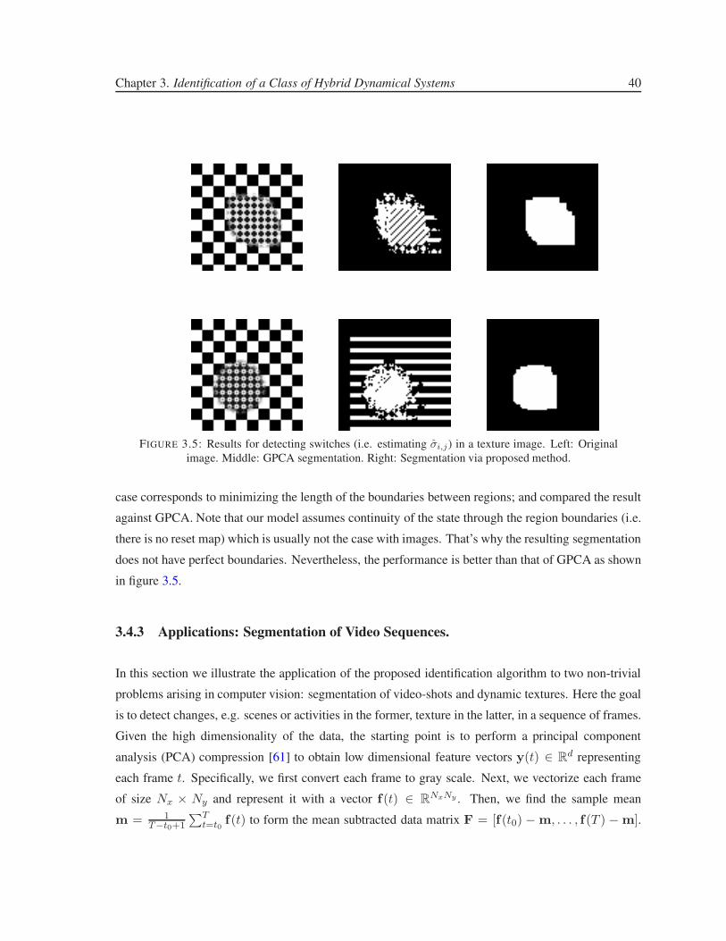
Chapter 3. Identification of a Class of Hybrid Dynamical Systems 40
FIGURE 3.5: Results for detecting switches (i.e. estimating σi,j) in a texture image. Left: Original
image. Middle: GPCA segmentation. Right: Segmentation via proposed method.
case corresponds to minimizing the length of the boundaries between regions; and compared the result
against GPCA. Note that our model assumes continuity of the state through the region boundaries (i.e.
there is no reset map) which is usually not the case with images. That’s why the resulting segmentation
does not have perfect boundaries. Nevertheless, the performance is better than that of GPCA as shown
in figure 3.5.
3.4.3 Applications: Segmentation of Video Sequences.
In this section we illustrate the application of the proposed identification algorithm to two non-trivial
problems arising in computer vision: segmentation of video-shots and dynamic textures. Here the goal
is to detect changes, e.g. scenes or activities in the former, texture in the latter, in a sequence of frames.
Given the high dimensionality of the data, the starting point is to perform a principal component
analysis (PCA) compression [61] to obtain low dimensional feature vectors y(t) ∈ Rd representing
each frame t. Specifically, we first convert each frame to gray scale. Next, we vectorize each frame
of size Nx × Ny and represent it with a vector f(t) ∈ RNxNy . Then, we find the sample mean
m = 1T−t0+1
∑Tt=t0
f(t) to form the mean subtracted data matrix F = [f(t0) − m, . . . , f(T ) − m].
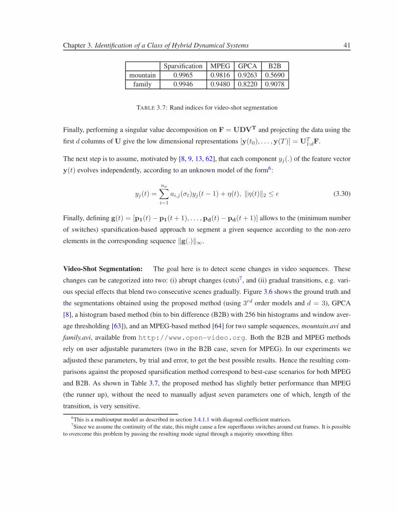
Chapter 3. Identification of a Class of Hybrid Dynamical Systems 41
Sparsification MPEG GPCA B2B
mountain 0.9965 0.9816 0.9263 0.5690
family 0.9946 0.9480 0.8220 0.9078
TABLE 3.7: Rand indices for video-shot segmentation
Finally, performing a singular value decomposition on F = UDVT and projecting the data using the
first d columns of U give the low dimensional representations [y(t0), . . . ,y(T )] = UT1:dF.
The next step is to assume, motivated by [8, 9, 13, 62], that each component yj(.) of the feature vector
y(t) evolves independently, according to an unknown model of the form6:
yj(t) =
na∑
i=1
ai,j(σt)yj(t − 1) + η(t), ‖η(t)‖2 ≤ ǫ (3.30)
Finally, defining g(t) = [p1(t)− p1(t + 1), . . . ,pd(t)−pd(t + 1)] allows to the (minimum number
of switches) sparsification-based approach to segment a given sequence according to the non-zero
elements in the corresponding sequence ‖g(.)‖∞.
Video-Shot Segmentation: The goal here is to detect scene changes in video sequences. These
changes can be categorized into two: (i) abrupt changes (cuts)7, and (ii) gradual transitions, e.g. vari-
ous special effects that blend two consecutive scenes gradually. Figure 3.6 shows the ground truth and
the segmentations obtained using the proposed method (using 3rd order models and d = 3), GPCA
[8], a histogram based method (bin to bin difference (B2B) with 256 bin histograms and window aver-
age thresholding [63]), and an MPEG-based method [64] for two sample sequences, mountain.avi and
family.avi, available from http://www.open-video.org. Both the B2B and MPEG methods
rely on user adjustable parameters (two in the B2B case, seven for MPEG). In our experiments we
adjusted these parameters, by trial and error, to get the best possible results. Hence the resulting com-
parisons against the proposed sparsification method correspond to best-case scenarios for both MPEG
and B2B. As shown in Table 3.7, the proposed method has slightly better performance than MPEG
(the runner up), without the need to manually adjust seven parameters one of which, length of the
transition, is very sensitive.
6This is a multioutput model as described in section 3.4.1.1 with diagonal coefficient matrices.7Since we assume the continuity of the state, this might cause a few superfluous switches around cut frames. It is possible
to overcome this problem by passing the resulting mode signal through a majority smoothing filter.
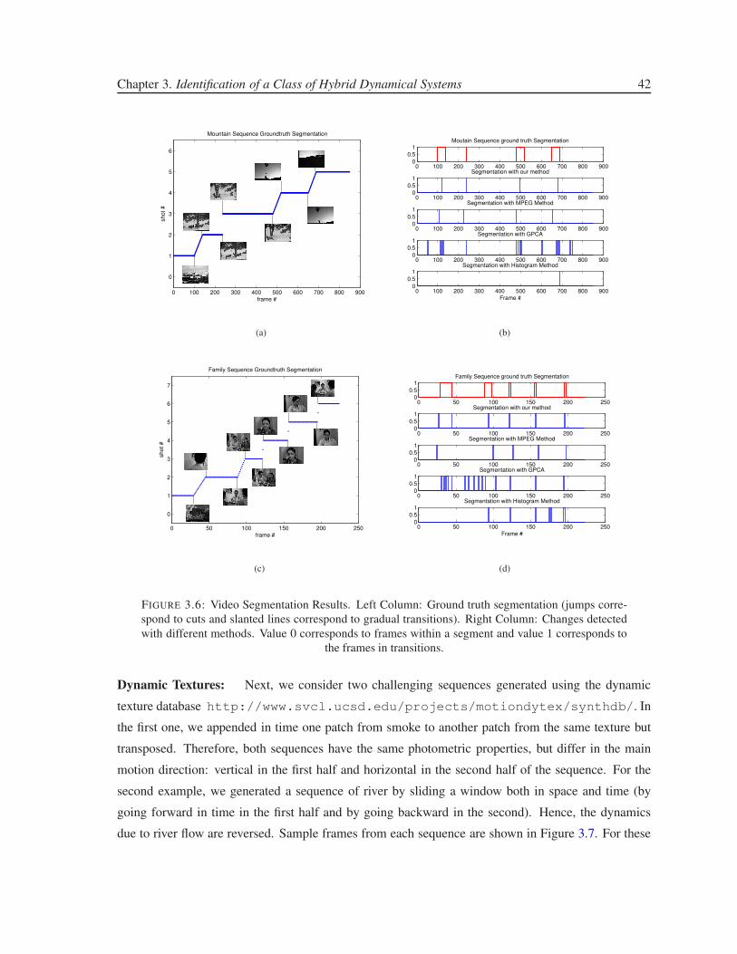
Chapter 3. Identification of a Class of Hybrid Dynamical Systems 42
0 100 200 300 400 500 600 700 800 900
0
1
2
3
4
5
6
Mountain Sequence Groundtruth Segmentation
frame #
sh
ot
#
(a)
0 100 200 300 400 500 600 700 800 9000
0.5
1Moutain Sequence ground truth Segmentation
0 100 200 300 400 500 600 700 800 9000
0.5
1Segmentation with our method
0 100 200 300 400 500 600 700 800 9000
0.5
1Segmentation with MPEG Method
0 100 200 300 400 500 600 700 800 9000
0.5
1Segmentation with GPCA
0 100 200 300 400 500 600 700 800 9000
0.5
1Segmentation with Histogram Method
Frame #
(b)
0 50 100 150 200 250
0
1
2
3
4
5
6
7
Family Sequence Groundtruth Segmentation
frame #
sh
ot
#
(c)
0 50 100 150 200 2500
0.5
1Family Sequence ground truth Segmentation
0 50 100 150 200 2500
0.5
1Segmentation with our method
0 50 100 150 200 2500
0.5
1Segmentation with MPEG Method
0 50 100 150 200 2500
0.5
1Segmentation with GPCA
0 50 100 150 200 2500
0.5
1Segmentation with Histogram Method
Frame #
(d)
FIGURE 3.6: Video Segmentation Results. Left Column: Ground truth segmentation (jumps corre-
spond to cuts and slanted lines correspond to gradual transitions). Right Column: Changes detected
with different methods. Value 0 corresponds to frames within a segment and value 1 corresponds to
the frames in transitions.
Dynamic Textures: Next, we consider two challenging sequences generated using the dynamic
texture database http://www.svcl.ucsd.edu/projects/motiondytex/synthdb/. In
the first one, we appended in time one patch from smoke to another patch from the same texture but
transposed. Therefore, both sequences have the same photometric properties, but differ in the main
motion direction: vertical in the first half and horizontal in the second half of the sequence. For the
second example, we generated a sequence of river by sliding a window both in space and time (by
going forward in time in the first half and by going backward in the second). Hence, the dynamics
due to river flow are reversed. Sample frames from each sequence are shown in Figure 3.7. For these

Chapter 3. Identification of a Class of Hybrid Dynamical Systems 43
FIGURE 3.7: Sample dynamic texture patches. Top: smoke, Bottom: river
sequences both histogram and MPEG methods failed to detect the cut since the only change is in the
dynamics. On the other hand, the proposed method (using 5th order models and d = 3) correctly
segmented both sequences. These results are summarized in Figure 3.8.
3.5 A Moments-Based Convex Optimization Approach
In this section we consider the problem of identifying hybrid systems from noisy input/output data
when the number of subsystems is known. In the noise free case, Vidal et al. [47, 50] proposed a
closed form solution to this problem. However, noise enters their formulation polynomially leading
to a nonconvex problem. In this section, by using ideas from polynomial optimization we reformulate
the problem in terms of probability distributions and moments. Our formulation, which is shown to be
equivalent to the original non-convex problem, requires to solve a rank minimization subject to LMI
constraints. Finally, we resort to a convex relaxation for dropping the rank to obtain a semidefinite
programming problem that can be solved efficiently.
The problem of interest here can formally be stated as follows:
Problem 4. Given input/output data over the interval [1, T ], a bound on the ℓ∞ norm of the noise
(i.e. ‖η‖∞ ≤ ǫ), and the number of submodels s, find a hybrid linear model of the form (3.1) that is
consistent with the a priori information and experimental data.
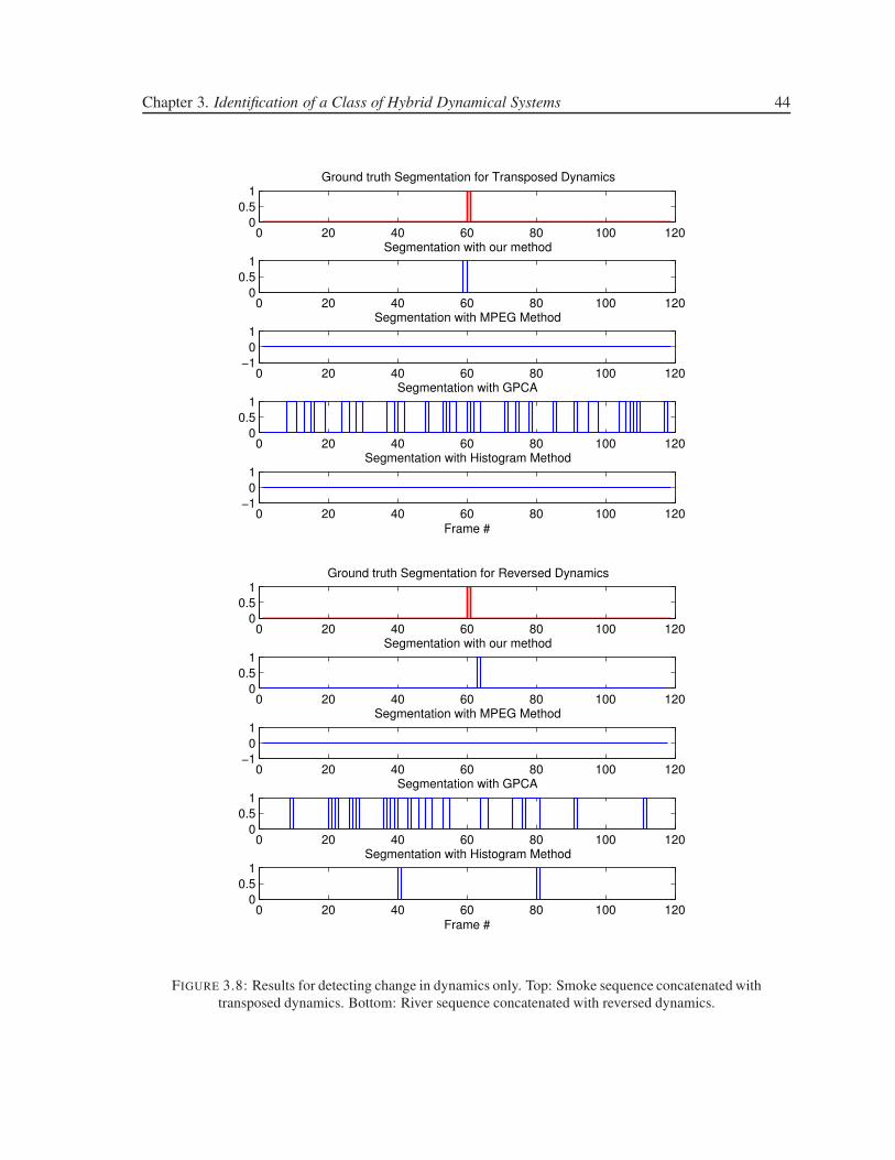
Chapter 3. Identification of a Class of Hybrid Dynamical Systems 44
0 20 40 60 80 100 1200
0.5
1Ground truth Segmentation for Transposed Dynamics
0 20 40 60 80 100 1200
0.5
1Segmentation with our method
0 20 40 60 80 100 120−1
0
1Segmentation with MPEG Method
0 20 40 60 80 100 1200
0.5
1Segmentation with GPCA
0 20 40 60 80 100 120−1
0
1Segmentation with Histogram Method
Frame #
0 20 40 60 80 100 1200
0.5
1Ground truth Segmentation for Reversed Dynamics
0 20 40 60 80 100 1200
0.5
1Segmentation with our method
0 20 40 60 80 100 120−1
0
1Segmentation with MPEG Method
0 20 40 60 80 100 1200
0.5
1Segmentation with GPCA
0 20 40 60 80 100 1200
0.5
1Segmentation with Histogram Method
Frame #
FIGURE 3.8: Results for detecting change in dynamics only. Top: Smoke sequence concatenated with
transposed dynamics. Bottom: River sequence concatenated with reversed dynamics.
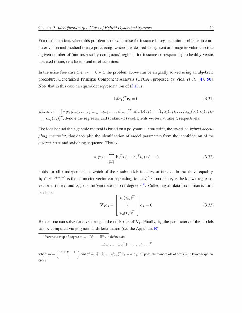
Chapter 3. Identification of a Class of Hybrid Dynamical Systems 45
Practical situations where this problem is relevant arise for instance in segmentation problems in com-
puter vision and medical image processing, where it is desired to segment an image or video clip into
a given number of (not necessarily contiguous) regions, for instance corresponding to healthy versus
diseased tissue, or a fixed number of activities.
In the noise free case (i.e. ηt = 0 ∀t), the problem above can be elegantly solved using an algebraic
procedure, Generalized Principal Component Analysis (GPCA), proposed by Vidal et al. [47, 50].
Note that in this case an equivalent representation of (3.1) is:
b(σt)Trt = 0 (3.31)
where rt = [−yt, yt−1, . . . , yt−na , ut−1, . . . , ut−nc ]T and b(σt) = [1, a1(σt), . . . , ana(σt), c1(σt),-
. . . , cnc(σt)]T , denote the regressor and (unknown) coefficients vectors at time t, respectively.
The idea behind the algebraic method is based on a polynomial constraint, the so-called hybrid decou-
pling constraint, that decouples the identification of model parameters from the identification of the
discrete state and switching sequence. That is,
ps(r) =
s∏
i=1
(biT rt) = cs
T νs(rt) = 0 (3.32)
holds for all t independent of which of the s submodels is active at time t. In the above equality,
bi ∈ Rna+nc+1 is the parameter vector corresponding to the ith submodel, rt is the known regressor
vector at time t, and νs(.) is the Veronese map of degree s 8. Collecting all data into a matrix form
leads to:
Vscs.=
νs(rt0)T
...
νs(rT )T
cs = 0 (3.33)
Hence, one can solve for a vector cs in the nullspace of Vs. Finally, bi, the parameters of the models
can be computed via polynomial differentiation (see the Appendix B).
8Veronese map of degree s, νs : Rn → R
m, is defined as:
νs([x1, . . . , xn]T ) = [. . . , ξs, . . .]T
where m =
(
s + n − 1s
)
and ξs .= x
s1
1 xs2
2 . . . xsn
n ,∑
si = s, e.g. all possible monomials of order s, in lexicographical
order.

Chapter 3. Identification of a Class of Hybrid Dynamical Systems 46
3.5.1 Main Results
In the presence of noise, the approach outlined above breaks down, since conditions (3.32) and (3.33)
no longer hold. Indeed, the noisy equivalent of (3.32) is given by:
ps(r, η) =
s∏
i=1
(biT rt) = cs
T νs(rt) = 0 (3.34)
where rt = [−yt + ηt, yt−1, . . . , yt−na , ut−1, . . . , ut−nc ]T . Proceeding as in the noiseless case, a
“noisy” data matrix Vs(r, η) can be built. However, finding the coefficients of each subsystem entails
now finding both an admissible noise sequence ηo and a vector co in the nullspace of Vs(r, ηo) such
that
Vs(r, ηo)co = 0 (3.35)
Since Vs is a polynomial function of the unknown noise terms η(t), this approach leads to a com-
putationally very challenging nonlinear, nonconvex optimization problem. However, as we show in
the sequel, by exploiting the method of the moments, (3.35) can be recast into a constrained rank
minimization form which in turn can be relaxed to an efficient convex optimization. We recall some
background results on polynomial optimization and problem of moments, which will be used to recast
the identification problem into a convex optimization form, in Appendices 2.2.1 and 2.2.2.
3.5.1.1 A Moments Based Convex Relaxation:
Consider the following rank minimization problem:
minimizeηt rankVs(rt, ηt)
subject to ‖ηt‖∞ ≤ ǫ(3.36)
Clearly, Problem 4 is solvable if and only if (3.36) admits a rank deficient solution. Indeed, in the case
where the order of each subsystem is precisely (na, nc) and Vs has generically full column rank (e.g.
enough data points have been collected from each subsystem), then there exists a noise sequence ηot
such that the right null space of Vs(rt, ηot ) has dimension 1. When some of the subsystems have order
lower than (na, nc) or the number of subsystems is overestimated, the dimension of the nullspace
of Vs is higher than 1 (see [47] for details). In that sense, minimizing the rank of Vs amounts to
searching for the simplest model that explains the data.
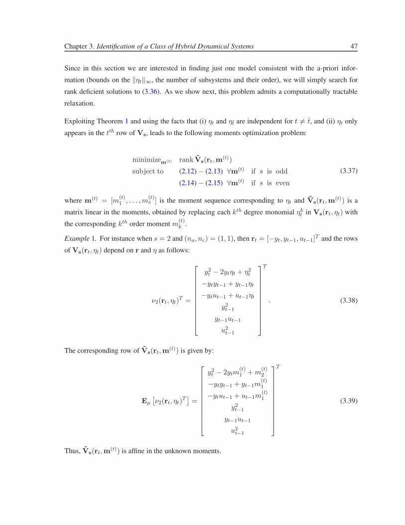
Chapter 3. Identification of a Class of Hybrid Dynamical Systems 47
Since in this section we are interested in finding just one model consistent with the a-priori infor-
mation (bounds on the ‖ηt‖∞, the number of subsystems and their order), we will simply search for
rank deficient solutions to (3.36). As we show next, this problem admits a computationally tractable
relaxation.
Exploiting Theorem 1 and using the facts that (i) ηt and ηt are independent for t 6= t, and (ii) ηt only
appears in the tth row of Vs, leads to the following moments optimization problem:
minimizem(t) rank Vs(rt,m(t))
subject to (2.12) − (2.13) ∀m(t) if s is odd
(2.14) − (2.15) ∀m(t) if s is even
(3.37)
where m(t) = [m(t)1 , . . . ,m
(t)s ] is the moment sequence corresponding to ηt and Vs(rt,m
(t)) is a
matrix linear in the moments, obtained by replacing each kth degree monomial ηkt in Vs(rt, ηt) with
the corresponding kth order moment m(t)k .
Example 1. For instance when s = 2 and (na, nc) = (1, 1), then rt = [−yt, yt−1, ut−1]T and the rows
of Vs(rt, ηt) depend on r and η as follows:
ν2(rt, ηt)T =
y2t − 2ytηt + η2
t
−ytyt−1 + yt−1ηt
−ytut−1 + ut−1ηt
y2t−1
yt−1ut−1
u2t−1
T
. (3.38)
The corresponding row of Vs(rt,m(t)) is given by:
Eµ
[
ν2(rt, ηt)T]
=
y2t − 2ytm
(t)1 + m
(t)2
−ytyt−1 + yt−1m(t)1
−ytut−1 + ut−1m(t)1
y2t−1
yt−1ut−1
u2t−1
T
(3.39)
Thus, Vs(rt,m(t)) is affine in the unknown moments.
Chapter 3. Identification of a Class of Hybrid Dynamical Systems 48
Note that Theorem 3 cannot be directly applied to show the equivalence of (3.36) and (3.37) since
rank is not a polynomial function. Nevertheless, as we show next, a result similar to Theorem 3 can
be obtained:
Theorem 8. There exists a rank deficient solution to problem (3.36) if and only if there exists a rank
deficient solution to problem (3.37). Moreover, if c belongs to the nullspace of the solution of (3.37)
then there exists a noise value η∗ with ‖η∗‖∞ ≤ ǫ such that c belongs to the nullspace of Vs(rt, η∗).
Proof. Assume that the minimum rank r1 in (3.36) is achieved by some sequence η∗t . Then Vs(rt,m∗(t))
with m∗(t) = [η∗t , (η∗t )2, . . . , (η∗t )s] (i.e. all distributions have point support) has rank r1 and m∗(t)
satisfies the LMI constraints. Hence the minimum rank obtained by solving (3.37) is less than or equal
to the minimum rank obtained by solving (3.36).
Consider now an optimal solution m∗(t) of (3.37). Note that, from Theorem 1, this guarantees the
existence of T measures µ∗(t), each supported on [−ǫ, ǫ]. Let c be in the nullspace of Vs(rt,m∗(t))
(i.e. Vs(rt,m∗(t))c = 0). Thus, for each row of Vs, Eµ∗(t) [νs(rt, ηt)] c = Eµ∗(t) [νs(rt, ηt)c] = 0.
By noting that νs(rt, ηt)c is a polynomial function of ηt (hence continuous) and µ∗(t) is supported on
[−ǫ, ǫ], we can invoke the mean value theorem for integration to conclude that there exist η∗t ∈ [−ǫ, ǫ]
for all t such that νs(rt, η∗t )c = 0.
Thus, whenever the nullspace of the solution of (3.36) is non-trivial, so is that of (3.37), which proves
the theorem.
An alternative way of obtaining an equivalent moment–based problem to (3.36) when Vs(rt, ηt) is
known to be rank deficient by one is to define the equivalent polynomial objective function
det[VsT (rt, ηt)Vs(rt, ηt)]. However, in this case one would need higher order (possibly infinite num-
ber of) moments of a multidimensional distribution since it is not clear how to exploit the indepen-
dence of noise terms while keeping the problem linear in moments. Although the rank objective is
non-convex, it has following advantages: (i) the equivalent moment based problem is finite dimen-
sional (i.e. it requires only finite moment matrices); (ii) there are efficient convex relaxations for
rank minimization; and (iii) extracting solutions requires only solving for the roots of a polynomial
in one variable whereas for the case with multidimensional distributions this is a non-trivial task. We
eloborate on the last two points next.
Although rank minimization is an NP–Hard problem, efficient convex relaxations are available. In
particular, good approximate solutions can be obtained by using a log–det heuristic [51] that relaxes
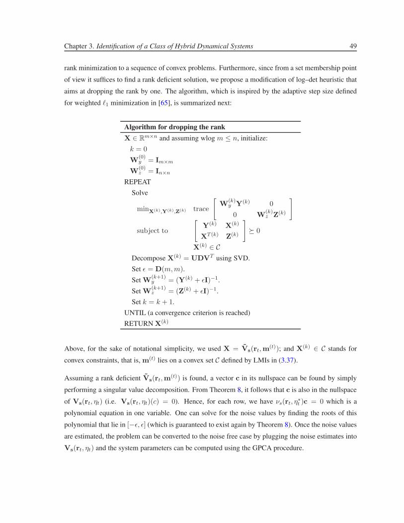
Chapter 3. Identification of a Class of Hybrid Dynamical Systems 49
rank minimization to a sequence of convex problems. Furthermore, since from a set membership point
of view it suffices to find a rank deficient solution, we propose a modification of log–det heuristic that
aims at dropping the rank by one. The algorithm, which is inspired by the adaptive step size defined
for weighted ℓ1 minimization in [65], is summarized next:
Algorithm for dropping the rank
X ∈ Rm×n and assuming wlog m ≤ n, initialize:
k = 0
W(0)y = Im×m
W(0)z = In×n
REPEAT
Solve
minX(k),Y(k),Z(k) trace
[
W(k)y Y(k) 0
0 W(k)z Z(k)
]
subject to
[
Y(k) X(k)
XT (k) Z(k)
]
� 0
X(k) ∈ C
Decompose X(k) = UDVT using SVD.
Set ǫ = D(m,m).
Set W(k+1)y = (Y(k) + ǫI)−1.
Set W(k+1)z = (Z(k) + ǫI)−1.
Set k = k + 1.
UNTIL (a convergence criterion is reached)
RETURN X(k)
Above, for the sake of notational simplicity, we used X = Vs(rt,m(t)); and X(k) ∈ C stands for
convex constraints, that is, m(t) lies on a convex set C defined by LMIs in (3.37).
Assuming a rank deficient Vs(rt,m(t)) is found, a vector c in its nullspace can be found by simply
performing a singular value decomposition. From Theorem 8, it follows that c is also in the nullspace
of Vs(rt, ηt) (i.e. Vs(rt, ηt)(c) = 0). Hence, for each row, we have νs(rt, η∗t )c = 0 which is a
polynomial equation in one variable. One can solve for the noise values by finding the roots of this
polynomial that lie in [−ǫ, ǫ] (which is guaranteed to exist again by Theorem 8). Once the noise values
are estimated, the problem can be converted to the noise free case by plugging the noise estimates into
Vs(rt, ηt) and the system parameters can be computed using the GPCA procedure.
Chapter 3. Identification of a Class of Hybrid Dynamical Systems 50
Remark 7. When the number of the submodels s is unknown, it is possible to search for minimum
number of submodels that explains the data. This can be accomplished with a simple iteration on s;
starting with s = 1 and increasing s up until a rank deficient solution to the problem (3.37) is found.
3.5.2 Illustrative Examples
In this section we use both an academic and a practical example to illustrate the effectiveness of the
proposed method.
3.5.2.1 Academic Example:
Consider a hybrid system that switches among the following three ARX subsystems
yt = 0.2yt−1 + 0.24yt−2 + 2ut−1 + ηt (Submodel 1)
yt = −1.4yt−1 − 0.53yt−2 + ut−1 + ηt (Submodel 2)
yt = 1.7yt−1 − 0.72yt−2 + 0.5ut−1 + ηt (Submodel 3)
modeled as
yt = p1(σt)yt−1 + p2(σt)yt−2 + p3(σt)ut−1 + ηt. (3.40)
where σt ∈ {1, 2, 3} depending on which model is active at time t. Experimental data was obtained
by running a simulation for T = 96 time steps with ‖η‖∞ = 0.25 where σt = 1 for t = [1, 32],
σt = 2 for t = [33, 64] and σt = 3 for t = [65, 96]. The parameter values used for the simulation are
shown in Table 3.8 together with the results obtained by our robust version of the algebraic method and
the original algebraic method of [50]. Figures 3.9 and 3.10 show the clustering of data into different
submodels. As seen there, the proposed method outperforms the method in [50]. Figures 3.11 and 3.12
show the absolute error given the identified model. The error values are quite large for the method in
[50] whereas they mostly satisfy the prior bound of ‖η‖∞ = 0.25 for the new method. Indeed, in
the latter case, the error exceeds the bound only at a single time instant. This is due to the convex
relaxation used to solve the original algebraic problem.
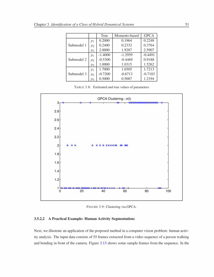
Chapter 3. Identification of a Class of Hybrid Dynamical Systems 51
True Moments-based GPCA
Submodel 1
p1 0.2000 0.1964 0.2248
p2 0.2400 0.2332 0.3764
p3 2.0000 1.9287 2.5907
Submodel 2
p1 -1.4000 -1.2959 -0.4491
p2 -0.5300 -0.4469 0.9188
p3 1.0000 1.0315 1.5262
Submodel 3
p1 1.7000 1.6505 1.7213
p2 -0.7200 -0.6713 -0.7103
p3 0.5000 0.5007 1.2194
TABLE 3.8: Estimated and true values of parameters
0 20 40 60 80 1001
1.2
1.4
1.6
1.8
2
2.2
2.4
2.6
2.8
3
GPCA Clustering− σ(t)
FIGURE 3.9: Clustering via GPCA.
3.5.2.2 A Practical Example: Human Activity Segmentation:
Next, we illustrate an application of the proposed method in a computer vision problem: human activ-
ity analysis. The input data consists of 55 frames extracted from a video sequence of a person walking
and bending in front of the camera. Figure 3.13 shows some sample frames from the sequence. In the
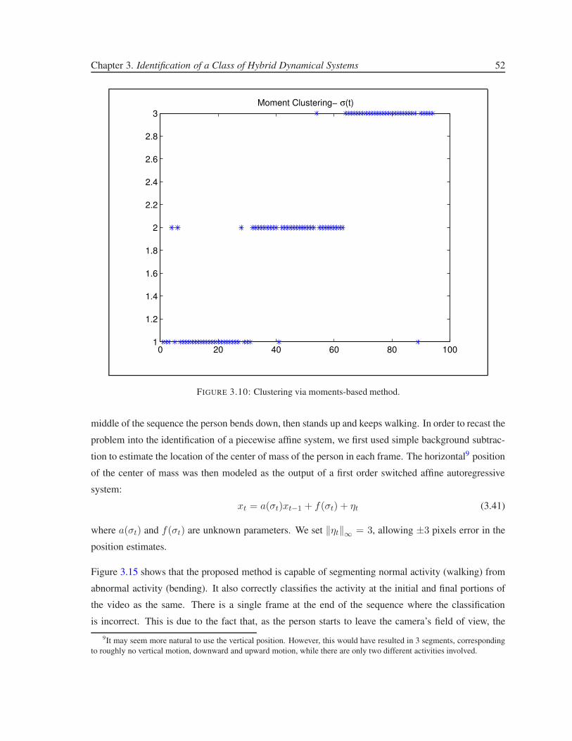
Chapter 3. Identification of a Class of Hybrid Dynamical Systems 52
0 20 40 60 80 1001
1.2
1.4
1.6
1.8
2
2.2
2.4
2.6
2.8
3
Moment Clustering− σ(t)
FIGURE 3.10: Clustering via moments-based method.
middle of the sequence the person bends down, then stands up and keeps walking. In order to recast the
problem into the identification of a piecewise affine system, we first used simple background subtrac-
tion to estimate the location of the center of mass of the person in each frame. The horizontal9 position
of the center of mass was then modeled as the output of a first order switched affine autoregressive
system:
xt = a(σt)xt−1 + f(σt) + ηt (3.41)
where a(σt) and f(σt) are unknown parameters. We set ‖ηt‖∞ = 3, allowing ±3 pixels error in the
position estimates.
Figure 3.15 shows that the proposed method is capable of segmenting normal activity (walking) from
abnormal activity (bending). It also correctly classifies the activity at the initial and final portions of
the video as the same. There is a single frame at the end of the sequence where the classification
is incorrect. This is due to the fact that, as the person starts to leave the camera’s field of view, the
9It may seem more natural to use the vertical position. However, this would have resulted in 3 segments, corresponding
to roughly no vertical motion, downward and upward motion, while there are only two different activities involved.
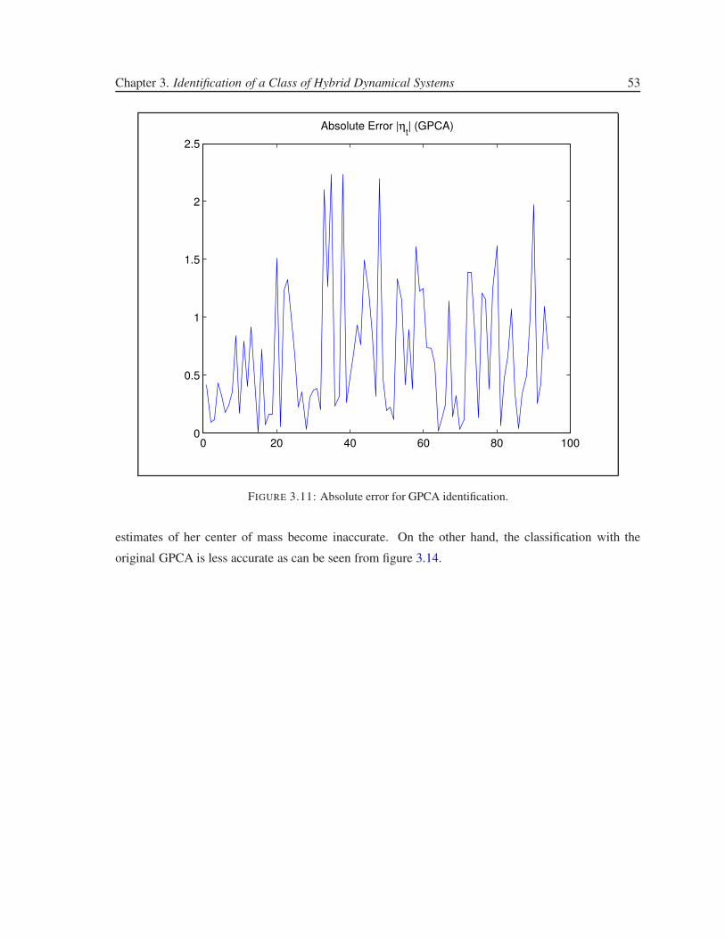
Chapter 3. Identification of a Class of Hybrid Dynamical Systems 53
0 20 40 60 80 1000
0.5
1
1.5
2
2.5
Absolute Error |ηt| (GPCA)
FIGURE 3.11: Absolute error for GPCA identification.
estimates of her center of mass become inaccurate. On the other hand, the classification with the
original GPCA is less accurate as can be seen from figure 3.14.

Chapter 3. Identification of a Class of Hybrid Dynamical Systems 54
0 20 40 60 80 1000
0.05
0.1
0.15
0.2
0.25
0.3
0.35
Absolute Error |ηt| (Moment)
FIGURE 3.12: Absolute error for moments-based identification.
frame 8 frame 23 frame 33 frame 50
FIGURE 3.13: Sample frames from the video.
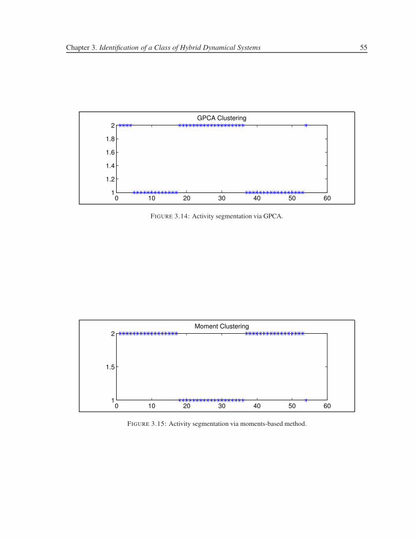
Chapter 3. Identification of a Class of Hybrid Dynamical Systems 55
0 10 20 30 40 50 601
1.2
1.4
1.6
1.8
2GPCA Clustering
FIGURE 3.14: Activity segmentation via GPCA.
0 10 20 30 40 50 601
1.5
2Moment Clustering
FIGURE 3.15: Activity segmentation via moments-based method.
Chapter 4
Model (In)validation for a Class of
Hybrid Dynamical Systems
4.1 Introduction and Motivation
As mentioned in the previous Chapter, hybrid systems, dynamical systems where continuous and
discrete states interact, are ubiquitous in many different contexts. Thus, during the past few years, a
considerable research effort has been devoted to the problem of identifying hybrid systems, leading
to several methods (see the excellent tutorial paper [46] for a summary of the main issues and recent
developments in the field). Since the identification problem is generically NP-Hard, the majority of
existing identification algorithms, including the ones presented in Chapter 3, are based on heuristics or
relaxations ([48, 66, 67, 68, 69]). Hence, a crucial step before using the resulting models, is to check
their validity against additional experimental data. Model (in)validation of Linear Time Invariant
(LTI) systems has been extensively addressed in the past two decades and both time and frequency
domain results are available in the literature (see for instance [70, 71, 72] and references therein). A
related line of research is model (in)validation of Linear Parameter Varying (LPV) systems ([73, 74])
where it is assumed that parameter values are measurable during the experiment and used as part of
a posteriori data during the (in)validation step. Finally, (in)validation of continuous-time nonlinear
models was addressed in [75] using sum of squares methods and barrier functions. However, to the
best of our knowledge, similar results for discrete-time switched linear systems with unknown switches
has not been considered, with the main difficulty here being the combination of noisy measurements
and an unknown mode signal.
56
Chapter 4. Model (In)validation for a Class of Hybrid Dynamical Systems 57
The main result of this chapter is a necessary and sufficient condition for a multi-input multi-output
switched affine autoregressive exogenous model to be (in)validated by the experimental data. Specif-
ically, given a nominal model and experimental input/output data, we provide certificates for the ex-
istence/nonexistence of a switching sequence such that the resulting output sequence interpolates the
given experimental data within a given noise bound. The starting point to obtain such certificates is to
recast the (in)validation problem as one of checking whether a semialgebraic set is empty. By using a
combination of recent results on moments-based sparse polynomial optimization and duality we show
that emptiness of this set is equivalent to strict positivity of the solution of a related, convex optimiza-
tion problem. In principle, checking this condition requires solving a sequence of convex optimization
problems involving increasingly large matrices. However, as we show in this chapter, if in the process
of solving these problems either a positive solution is found or the rank of certain matrices formed
using the solution to the dual problem ceases to increase (the so-called flat extension property), then
the process terminates with either an invalidation or a consistency certificate. A salient feature of the
proposed approach is its ability to exploit the inherently sparse structure of the optimization problem
to substantially reduce its computational complexity.
In the second portion of the chapter, these results are illustrated both with academic examples and a
non-trivial problem arising in computer vision: activity monitoring. Typically, a visual surveillance
system captures high volume data streams from multiple cameras. However, interesting (e.g. ab-
normal) activities are rare. Thus, it is important to be able to automatically eliminate the “normal”
behavior and trigger an appropriate response when something potentially interesting or “abnormal”
occurs. As we show in Section 4.4.2, this problem can be recast into a piecewise–affine model invali-
dation form and solved using the framework developed in this chapter.
4.2 (In)validating MIMO SARX Models
In this section we formally state the problem under consideration and show that it can be reduced to a
polynomial optimization over a semialgebraic set. In turn, this allows for exploiting the results briefly
discussed in section 2.2.1 to obtain computationally tractable (in)validation certificates.

Chapter 4. Model (In)validation for a Class of Hybrid Dynamical Systems 58
4.2.1 Problem Statement
In this chapter, we consider multi-input, multi-output (MIMO) switched affine autoregressive exoge-
nous (SARX) models of the form:
yt =∑na
k=1 Ak(σt)yt−k
+∑nc
k=1 Ck(σt)ut−k + f(σt)
yt = yt + ηt
(4.1)
where ut ∈ Rnu is the input, yt ∈ R
ny is the measured output corrupted by the noise ηt ∈ Rny ,
and σt ∈ Ns is the discrete mode signal indicating which of the s submodels is active at time
t. We do not make any dwell-time assumptions, hence the mode signal σt can switch arbitrar-
ily among the s submodels Gi, each of which is associated with the set of its coefficient matrices
{A1(i), . . . ,Ana(i),C1(i), . . . ,Cnc(i), f(i)}.
The model (in)validation problem for the setup described above and shown in Figure 4.1 can be for-
mally stated as follows:
Problem 5. Given a nominal hybrid model of the form (4.1) together with its s submodels G1, . . . , Gs,
an a priori bound ǫ on noise, and experimental data {ut, yt}Tt=t0 , determine whether or not the a
priori information and the a posteriori experimental data are consistent, i.e. whether the consistency
set
T (η, σ) = {||ηt||∞ ≤ ǫ, σt ∈ Ns
subject to (4.1) ∀t ∈ [t0, T ]}
is nonempty.
Since T (η, σ) contains all possible noise and mode signal sequences that can explain the observed
data, clearly establishing that T (η, σ) = ∅ is equivalent to invalidating the model.
4.2.2 A Convex Certificate for (In)validating MIMO SARX Models
Next, we present the main result of the chapter, showing that a necessary and sufficient condition for
the model to be invalidated by the experimental data is strict positivity of the solution to a related
convex optimization problem. We begin by constructing a semialgebraic set T ′(η) and showing its
equivalence, in a sense to become clear later, to the consistency set T (η, σ). To this effect, assume
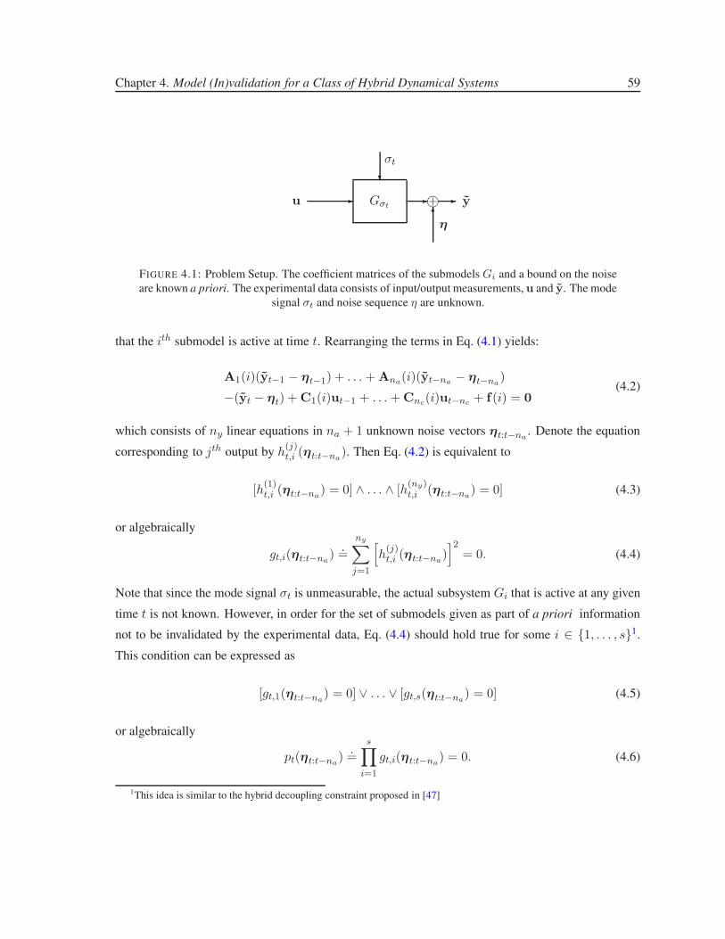
Chapter 4. Model (In)validation for a Class of Hybrid Dynamical Systems 59
-u
?
σt
Gσt- h+ - y
6η
FIGURE 4.1: Problem Setup. The coefficient matrices of the submodels Gi and a bound on the noise
are known a priori. The experimental data consists of input/output measurements, u and y. The mode
signal σt and noise sequence η are unknown.
that the ith submodel is active at time t. Rearranging the terms in Eq. (4.1) yields:
A1(i)(yt−1 − ηt−1) + . . . + Ana(i)(yt−na − ηt−na)
−(yt − ηt) + C1(i)ut−1 + . . . + Cnc(i)ut−nc + f(i) = 0(4.2)
which consists of ny linear equations in na + 1 unknown noise vectors ηt:t−na. Denote the equation
corresponding to jth output by h(j)t,i (ηt:t−na
). Then Eq. (4.2) is equivalent to
[h(1)t,i (ηt:t−na
) = 0] ∧ . . . ∧ [h(ny)t,i (ηt:t−na
) = 0] (4.3)
or algebraically
gt,i(ηt:t−na)
.=
ny∑
j=1
[
h(j)t,i (ηt:t−na
)]2
= 0. (4.4)
Note that since the mode signal σt is unmeasurable, the actual subsystem Gi that is active at any given
time t is not known. However, in order for the set of submodels given as part of a priori information
not to be invalidated by the experimental data, Eq. (4.4) should hold true for some i ∈ {1, . . . , s}1.
This condition can be expressed as
[gt,1(ηt:t−na) = 0] ∨ . . . ∨ [gt,s(ηt:t−na
) = 0] (4.5)
or algebraically
pt(ηt:t−na)
.=
s∏
i=1
gt,i(ηt:t−na) = 0. (4.6)
1This idea is similar to the hybrid decoupling constraint proposed in [47]
Chapter 4. Model (In)validation for a Class of Hybrid Dynamical Systems 60
Next we use the equalities above to define a semialgebraic set and establish its relationship with the
consistency set T :
Proposition 1. Let
T ′(η).=
{
η | ft,j(η(j)t ) ≥ 0 ∀t ∈ [0, T ], j ∈ Nnyand
pt(ηt:t−na) = 0 ∀t ∈ [na, T ]
}
.
where
ft,j(η(j)t )
.= ǫ2 −
[
η(j)t
]2
Then, T (η, σ) is empty if and only if T ′(η) is empty.
Proof. Follows from the construction of T ′(η) and the fact that |η(j)t | ≤ ǫ ⇐⇒ ft,j(η
(j)t ) ≥ 0
At this point, one can use the Positivstellenstaz and derive sum of squares certificates for the emptiness
of T ′(η), as proposed in [76]. However, as we show next, adopting a dual approach based on the theory
of moments allows for exploiting the inherently sparse structure of the problem. In order to pursue
this approach, start by considering the following optimization problem:
o∗ = minη
∑Tt=na
pt(ηt:t−na)
s.t.
ft,j(η(j)t ) ≥ 0 ∀t ∈ [0, T ], j ∈ Nny .
(4.7)
Note that o∗ ≥ 0, since the objective function in (4.7) is a sum of squares polynomial2 . Further, if
T ′(η) is non-empty, then there exist a noise sequence η∗ for which (4.7) attains its minimum o∗ = 0.
Equivalently, o∗ > 0 ⇐⇒ T ′(η) = ∅.
Proposition 2. Problem (4.7) above satisfies the running intersection property.
Proof. Consider the T − na + 1 subsets Ik of the variables η0:T where each Ik contains only the
variables ηk:k+na. One can associate each ft,j with I0 for t ≤ na and with It−na for t > na. The
collection Ikj formed by repeating each Ik, ny times, satisfies (2.27) hence the running intersection
property in Definition 1 holds.
2since it is formed by multiplication and addition of SOS polynomials in (4.4), and the cone of SOS polynomials is
closed under these operations.
Chapter 4. Model (In)validation for a Class of Hybrid Dynamical Systems 61
Next, we use results from the theory of moments to obtain a convex problem where the objective and
constraints have affine (rather than polynomial) dependence on the data and exploits sparsity. Consider
the related moments-based optimization:
d∗N = minm
∑Tt=na
lt(mt−na:t)
s.t.
MN (mt−na:t) � 0 ∀t ∈ [na, T ]
LN (ft,jmt−na:t) � 0 ∀t ∈ [na + 1, T ], j ∈ Nny
LN (ft,jm0:na) � 0 ∀t ∈ [0, na], j ∈ Nny
(4.8)
where each lt is the linear functional of moments defined as lt(mt−na:t).= E
{
pt(ηt:t−na)}
, E de-
notes expectation and where MN and LN are the moments and localization matrices associated with a
truncated moments sequence containing terms up to order 2N with N ≥ s. Clearly d∗N ≥ 0, since the
objective function in (4.7) is a sum of squares polynomial, and, from Theorem 4, d∗N ↑ o∗ as N → ∞.
These observations lead to the following necessary and sufficient conditions for (in)validation:
Proposition 3. The following statements are equivalent:
(i) The consistency set T ′(η) is empty
(ii) There exists some finite No such that d∗No> 0
(iii) The solution r∗ to the following optimization problem is strictly greater than zero:
r∗ = minm
∑Tt=na
lt(mt−na:t)
s.t.
Ms(mt−na:t) � 0 ∀t ∈ [na, T ]
rank [Ms(mt−na:t)] = 1 ∀t ∈ [na, T ]
Ls(ft,jmt−na:t) � 0 ∀t ∈ [na + 1, T ], j ∈ Nny
Ls(ft,jm0:na) � 0 ∀t ∈ [0, na], j ∈ Nny
(4.9)
where each of the T − na + 1 moments sequences mt−na:t, t ∈ [na, T ], contains moments up
to order 2s (i.e. two times number of submodels).
Proof. (i)⇔(ii) Recall that T ′(η) = ∅ ⇐⇒ o∗ > 0. Since d∗N ↑ o∗ as N → ∞, if o∗ > 0, there exist
No such that d∗No> 0. On the other hand, if d∗No
> 0 then o∗ > 0 since d∗No< o∗. Hence, T ′(η) is
empty.
Chapter 4. Model (In)validation for a Class of Hybrid Dynamical Systems 62
(i)⇔(iii) To prove this equivalence, we show that r∗ in (4.9) is equal to o∗ in (4.7). Assume η∗ is an
optimizer of (4.7), then the moments of the distribution µ∗ with point support at η∗ is feasible for (4.9)
with the same objective value which implies r∗ ≤ o∗. On the other hand, if m∗ is a minimizer of
(4.9), the rank condition implies that there is a corresponding measure µ∗ with point support, say at
η∗. Since this value of η∗ is a feasible point of (4.7), o∗ ≤ r∗. Therefore, r∗ = o∗ from which we
conclude that r∗ > 0 is equivalent to (i).
Note that by forming a single block diagonal matrix containing all LMI constraints in (4.8), it can be
transformed into the standard dual form of semidefinite programs. That is:
d∗N = infm bTm + co
s.t.∑
α∈I Aαmα � C
(4.10)
where I is the set of the multi-indexes of all moments that occur in (4.8) except the zeroth moment
m0 = 1 which is used to form the constant terms C and co.
Remark 8. It is important to highlight the reduction achieved by employing the running intersec-
tion property while forming the optimization problem (4.8). The conventional moment relaxation
of order N in [41] would require O((Tny + ny)2N ) variables with a moment matrix of the size
(
N + Tny + ny
Tny + ny
)
. On the other hand, (4.8) involves only O((nany + ny)2N ) variables with
T − na + 1 moment matrices of the size
(
N + nany + ny
nany + ny
)
where, in general, the length of the
experimental data T is substantially larger than the order of the regressor na (i.e. na ≪ T ).
4.3 Numerical Considerations
From Proposition 3 it follows that (in)validation/validation certificates can be obtained, for instance,
by solving a sequence of problems with increasing N until either a solution with d∗ > 0 is found
(in which case the data invalidates the model) or condition (iii) fails, in which case the data record
is consistent with the model and a-priori information. However, a potential numerical difficulty here
stems from the fact that in practice d∗ = 0 is never reached since there is no closed form solution to
the problem and numerical solvers terminate when the duality gap drops below a certain level. Thus,
from a practical standpoint, more useful conditions can be obtained by examining the primal problem,
Chapter 4. Model (In)validation for a Class of Hybrid Dynamical Systems 63
which can be written as
p∗N = maxX < C,X > +co
s.t.
< Aα,X >= bα ∀α ∈ I
X � 0
(4.11)
where, without loss of generality, X can be chosen to have the same block-diagonal structure that
Aαs and C. Note that, from duality, p∗N ≤ d∗N , and hence p∗N > 0 provides an invalidation certificate.
In fact if problem (4.11) is feasible, strong duality holds [44]. Thus p∗N > 0 is strictly equivalent to
d∗N > 0, leading to the following result:
Proposition 4. The consistency set T ′(η) is empty if and only if p∗No> 0 for some finite No.
Proof. Follows directly from strong duality and Proposition 3.
Let dN and pN be the numerical solutions to problems (4.8) and (4.11) respectively, obtained using
a standard SDP solver. As noted before, in practice, one always has dN > 0. Thus it can be hard
to ascertain whether conditions (ii) or (iii) in Proposition 3 fail. On the other hand, p > 0 is an
invalidation certificate.
Remark 9. A certificate that the existing data record is consistent with the model and a priori as-
sumptions can be obtained by resorting to a variation of the so-called flat extension property for
sparse polynomial optimization stated in [44]. In particular, if for some N , p ≤ 0 and the dual
solution satisfies rank[
MN (m∗0:na
)]
= 1; rank[
MN (m∗t−na:t−1)
]
= 1 and rank[
MN (m∗t−na:t)
]
=
rank[
MN−2(m∗t−na:t)
]
∀t ∈ [na, T ] where m∗ denotes an optimal solution of (4.8), then this certi-
fies that o∗ = d∗N = 0; hence T ′(η) is not empty.
Remark 10. It is also worth pointing out that all of the results above (including the running intersection
property) hold true in the presence of bounded parametric model uncertainty. For instance, if ai(k, l)
is an entry in one of the coefficient matrices of the ith submodel, it is possible to use ai(k, l) + δi(k, l)
with |δi(k, l)| ≤ δ∗ in the a priori model. This only requires additional variables in the optimization
problem.

Chapter 4. Model (In)validation for a Class of Hybrid Dynamical Systems 64
4.4 Illustrative Examples
In this section we illustrate the effectiveness of the proposed method both using academic examples
and a computer vision application. In all cases, we used the moments relaxation corresponding to
N = s and the resulting SDP problem was solved using SEDUMI [16].
4.4.1 Academic Examples
We consider the ARX submodels:
yt = 0.2yt−1 + 0.24yt−2 + 2ut−1 (G1)
yt = −1.4yt−1 − 0.53yt−2 + ut−1 (G2)
yt = 1.7yt−1 − 0.72yt−2 + 0.5ut−1 (G3)
and the measurement equation:
yt = yt + ηt. (4.12)
We ran different sets of simulations investigating different sources of model mismatch. In all cases,
we collected input/output data {ut, yt} for t ∈ [0, 96] and tried to (in)validate the a priori model.
In all experiments, when we used data inconsistent with the a priori information, p∗ turned out to
be positive. Hence, we correctly invalidated the model in each of such cases. On the other hand,
whenever the a priori information was consistent with a posteriori data, we had p∗ < 0.
Example 2. (Submodel mismatch) For the first set of experiments, we generated input/output data using
different subsets of {G1, G2, G3} with a random switching sequence σt and with uniform random
noise ||ηt|| ≤ 0.5. The noise used in the experiments was within the a priori noise bound. We
used both correct and incorrect a priori submodel sets. Hence, the model should be invalid when a
submodel that is not contained in the a priori submodel set is used in the actual experiment. The
results are summarized in Table 4.1.
Example 3. (Noise bound mismatch) For this example, we generated input/output data using different
subsets of {G1, G2, G3} with a random switching sequence σt and with uniform random noise ||ηt|| ≤
ǫ. The a priori submodel set and the actual submodel set used in the experiment were the same. The
source of invalidation was the actual noise level exceeding the a priori bound. The results of this set
of experiments are summarized in Table 4.2.
Chapter 4. Model (In)validation for a Class of Hybrid Dynamical Systems 65
A priori Actual Result
G1, G2, G3 G1, G2, G3 not invalidated
G1, G2, G3 G1, G2 not invalidated
G1, G2 G1, G2, G3 invalidated
G1, G2 G2 not invalidated
G1, G2, G3 G1 not invalidated
G1, G2 G2, G3 invalidated
TABLE 4.1: Invalidation results for example 2. The values of p were respectively −3.8441e − 008,
−8.2932e− 009, 0.8585, −5.4026e− 008, −1.5490e− 007 and 0.7566.
Submodels A priori ǫ Actual ǫ Result
G1, G2, G3 0.5 1 invalidated
G1, G2, G3 0.8 1 invalidated
G1, G2, G3 1.2 1 not invalidated
G1, G2 0.5 1 invalidated
G1, G2 0.8 1 invalidated
G1, G2 1.2 1 not invalidated
TABLE 4.2: Invalidation results for example 3. The values of p were respectively 0.0724, 0.0035,
−5.1810e− 007, 0.0737, 0.0034 and −1.4930e− 007.
Example 4. (Submodel perturbation) For this set of experiments, we generated input/output data by
perturbing the coefficients of a priori submodels {G1, G2, G3}, and again using a random switching
sequence σt and uniformly sampled random noise ||ηt|| ≤ 0.5. We denote the submodel whose
coefficient values are perturbed by e percent of their original values as Gi + ∆e. This case is more
challenging than the one considered in Example 2 since the dynamics are similar. Nevertheless, we
could invalidate in each of our trials. The results for this example are summarized in Table 4.3.
A priori Actual Result
G1, G2, G3 G1 + ∆5, G2 + ∆5, G3 + ∆5 invalidated
G1, G2, G3 G1 + ∆2, G2 + ∆2, G3 + ∆2 invalidated
G1, G2, G3 G1 + ∆1, G2 + ∆1, G3 + ∆1 invalidated
G1, G2 G1 + ∆5, G2 + ∆5 invalidated
G1, G2 G1 + ∆2, G2 + ∆2 invalidated
G1, G2 G1 + ∆1, G2 + ∆1 invalidated
G1, G2 G1 + ∆2 invalidated
TABLE 4.3: Invalidation results for example 4. The values of p were ,respectively, 0.8963, 0.0997,
0.0080, 0.0308, 2.8638e− 004, 2.9069e− 006 and 6.2061e− 006.
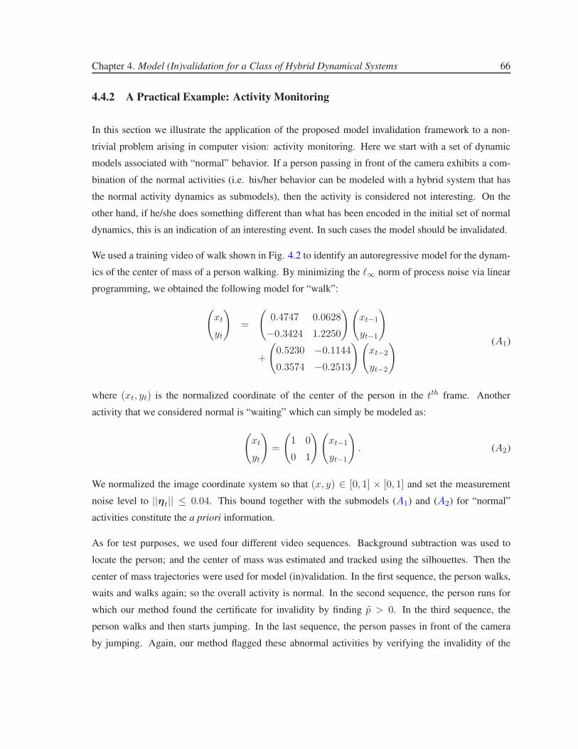
Chapter 4. Model (In)validation for a Class of Hybrid Dynamical Systems 66
4.4.2 A Practical Example: Activity Monitoring
In this section we illustrate the application of the proposed model invalidation framework to a non-
trivial problem arising in computer vision: activity monitoring. Here we start with a set of dynamic
models associated with “normal” behavior. If a person passing in front of the camera exhibits a com-
bination of the normal activities (i.e. his/her behavior can be modeled with a hybrid system that has
the normal activity dynamics as submodels), then the activity is considered not interesting. On the
other hand, if he/she does something different than what has been encoded in the initial set of normal
dynamics, this is an indication of an interesting event. In such cases the model should be invalidated.
We used a training video of walk shown in Fig. 4.2 to identify an autoregressive model for the dynam-
ics of the center of mass of a person walking. By minimizing the ℓ∞ norm of process noise via linear
programming, we obtained the following model for “walk”:
(
xt
yt
)
=
(
0.4747 0.0628
−0.3424 1.2250
)(
xt−1
yt−1
)
+
(
0.5230 −0.1144
0.3574 −0.2513
)(
xt−2
yt−2
) (A1)
where (xt, yt) is the normalized coordinate of the center of the person in the tth frame. Another
activity that we considered normal is “waiting” which can simply be modeled as:
(
xt
yt
)
=
(
1 0
0 1
)(
xt−1
yt−1
)
. (A2)
We normalized the image coordinate system so that (x, y) ∈ [0, 1] × [0, 1] and set the measurement
noise level to ||ηt|| ≤ 0.04. This bound together with the submodels (A1) and (A2) for “normal”
activities constitute the a priori information.
As for test purposes, we used four different video sequences. Background subtraction was used to
locate the person; and the center of mass was estimated and tracked using the silhouettes. Then the
center of mass trajectories were used for model (in)validation. In the first sequence, the person walks,
waits and walks again; so the overall activity is normal. In the second sequence, the person runs for
which our method found the certificate for invalidity by finding p > 0. In the third sequence, the
person walks and then starts jumping. In the last sequence, the person passes in front of the camera
by jumping. Again, our method flagged these abnormal activities by verifying the invalidity of the
Chapter 4. Model (In)validation for a Class of Hybrid Dynamical Systems 67
frame4 frame15 frame26 frame38 frame49
FIGURE 4.2: Training sequence used in identification of the submodel (A1) for walking.
models. Sample frames from the sequences are shown in Fig. 4.3 and the results are summarized in
Table 4.4.
A priori Actual Result
walk, wait walk, wait not invalidated
walk, wait run invalidated
walk, wait walk, jump invalidated
walk, wait jump invalidated
TABLE 4.4: Invalidation results for activity monitoring. The values of p were, respectively,
−2.3303e− 008, 2.3707e− 005, 5.0293e− 007, and 1.5998e− 006.
4.5 Conclusions
In this chapter we considered the model (in)validation problem for switched ARX systems with un-
known switches. Given a nominal model, a bound on the measurement noise and experimental input
output data, we provided a necessary and sufficient condition that certifies the existence/nonexistence
of admissible noise and switching sequences such that the resulting output sequence interpolates the
given experimental data within the noise bound. In principle, computing these certificates entails solv-
ing a sequence of convex optimization problems involving increasingly large matrices. However, as
we show here, if in the process of solving these problems either a positive solution is found or the so-
called flat extension property holds, then the process terminates with a certificate that either the model
has been invalidated (first case) or that the experimental data is indeed consistent with the model and
a–priori information. By using duality, the proposed approach exploits the inherently sparse structure
of the optimization problem to substantially reduce its computational complexity. The effectiveness of
the proposed method was illustrated using both academic examples and a non-trivial problem arising
in computer vision: activity monitoring.
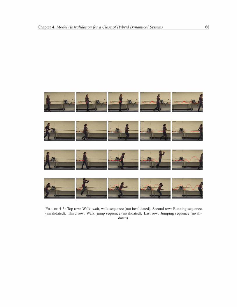
Chapter 4. Model (In)validation for a Class of Hybrid Dynamical Systems 68
frame5 frame20 frame30 frame45 frame63
frame2 frame7 frame14 frame19 frame24
frame4 frame16 frame28 frame40 frame55
frame4 frame15 frame27 frame40 frame55
FIGURE 4.3: Top row: Walk, wait, walk sequence (not invalidated). Second row: Running sequence
(invalidated). Third row: Walk, jump sequence (invalidated). Last row: Jumping sequence (invali-
dated).
Chapter 5
Clustering Data into Multiple Unknown
Subspaces
In this chapter, we deal with static data and we try to cluster the data such that the data within each
cluster lie on a subspace of the ambient space. This type of subspace clustering is relevant to many
computer vision problems such as affine motion segmentation, face clustering under varying illumi-
nation, and image, video and dynamic texture segmentation. The subspace clustering problem and the
problem of switched affine dynamical system identification have a quite similar structure. Hence, as
we show next, methods developed for one can be easily modified to be used for the other. In particular,
in section 5.1, we consider the case where temporal (spatial) ordering of the data points matters and
show that utilizing the order dependence it is possible to develop more robust segmentation algorithms
based on sparsification. In the second part (section 5.2), we consider the case where ordering does not
matter. We build upon an algebraic method ([8]) which is quite sensitive to noise and show that it is
possible to significantly reduce the noise resilience by combining elements from convex analysis and
the problem of moments. Extensions to algebraic surfaces other than subspaces are also presented.
69
Chapter 5. Clustering Data into Multiple Unknown Subspaces 70
5.1 Sequential Sparsification for Change Detection
5.1.1 Introduction and Motivation
Change detection is a very general concept that is encountered in many areas of computer vision.
From edge detection to video segmentation or image segmentation, a variety of computer vision tasks
can be considered as change detection problems with different interpretations of change. Hence, we
believe that a general purpose change detection method with only a few adjustable parameters will be
valuable. This section takes a step in this direction by exploiting sparsification based optimization.
Under the assumption that there exists an underlying piecewise affine model (e.g. vectors are clustered
in different subspaces), our main objective is to find when the model changes from one mode to another
and, at the same time, learn the parameters of the model. Hybrid piecewise affine models [8, 9] and
mixture models [12, 13, 14] have been the object of considerable attention in the past few years.
Although some of the work (for instance [13]) assumes a fixed number of models, one of the main
problems when working with hybrid models is that the number of models is usually unknown. [8]
provides a closed form algebraic solution for the noise free case, but the estimation of the number of
models usually fails when the data is noisy. As we show in this section, assuming a bound on the noise
level, allows for recasting the problem into a robust optimization form where the objective is to find
the minimum number of clusters (i.e. the simplest model to represent the data). A second point where
our method departs from existing clustering techniques is that we make explicit use of the sequential
nature of the data. For example, neighboring pixels in an image or consecutive frames in a video
sequence are more likely to be within the same segment, and thus imposing continuity of the clusters
leads to improved robustness.
Our main result shows that the robust segmentation problem can be recast into a change detection
form, where the goal is to detect points where the underlying hybrid model switches modes, or, equiv-
alently, to detect changes in the affine parameters describing the model. In principle, detecting these
changes can be hard when the measurements are corrupted by noise. However, as we show, this can be
robustly accomplished by searching for models that explain the observed data with the lowest possible
number of switches (e.g. looking for segmentations that maximize the length of subsequences). This
is equivalent to searching for descriptions that maximize the sparsity of the vector of first order tem-
poral parameter differences, since each non-zero element of this vector corresponds to a switch. This
allows us to proceed as in the dynamic case (see Section 3.4 for details). By exploiting the recently

Chapter 5. Clustering Data into Multiple Unknown Subspaces 71
developed results on signal sparsification, we obtain efficient, computationally tractable segmentation
algorithms.
5.1.2 Segmentation via Sparsification
In this section we consider the problem of segmenting vector valued sequences {x(t)}Tt=0 that are
generated by an affine parametric hybrid model with unknown parameters. Specifically, the models
that we consider have the following form:
H : f(
pσ(t), {x(k)}t+jk=t−i
)
= 0 (5.1)
where f is an affine function1 of the parameter vector pσ(t) which takes values from a finite unknown
set according to a piecewise constant function σ(t). Here i and j are positive integers that account for
the memory of the model (e.g. j = 0 corresponds to a causal model, or i = j = 0 corresponds to a
memoryless model).
We say that there exists a change at time t if σ(t) 6= σ(t + 1). Hence segmentation of a given
sequence into subsequences is equivalent to finding how many times and when these changes occur.
The segmentation problem can be formally stated as follows:
Problem 6. Given a sequence{
x(t) ∈ Rd}T
t=1generated by a hybrid parametric model H of the
form (5.1) find the minimum number of segments (i.e. subsequences) {Si}Ni=1 where on each Si =
{x(t)}Ti+1−1t=Ti
, σ(t) is constant and T1 = 1, TN+1 − 1 = T .
This is a difficult problem, since neither the segmentation nor the parameters of the hybrid model are
known. In order to overcome this difficulty, we consider the sequence of first order differences of the
time varying parameters p(t), given by
g(t) = p(t) − p(t + 1) (5.2)
Clearly, since a non-zero element of this sequence corresponds to a change, the sequence should be
sparse having only N −1 non-zero elements out of T . Next, in order to account for noise we introduce
a noise term η(t), satisfying ‖η‖∗ ≤ ǫ, where ‖.‖∗ denotes a norm relevant to the specific problem
1That is:
f(
pσ(t), {x(k)}t+j
k=t−i
)
= A(x)pσ(t) + b(x)
Chapter 5. Clustering Data into Multiple Unknown Subspaces 72
under consideration and ǫ is an upper bound on the noise level. In this context, Problem 6 can be recast
as an optimization problem as follows:
minimizep(t),η(t) ‖{g}‖l0
subject to f(
p(t), {x(k)}t+jk=t−i
)
= η(t) ∀t
‖{η}‖∗ ≤ ǫ
(5.3)
2 Here l0 is a quasinorm that counts non-zero elements (i.e. minimizing l0 norm is the same as
maximizing sparsity) and can be approximated by the l1 norm, leading to a linear cost function. When
f is an affine function of p(t), (5.3) has a convex feasibility set F . Thus, using the l1 norm leads to
a convex, computationally tractable relaxation. Further, Fazel et al. proposed an iterative procedure
in [51] and [56] to improve the solution obtained by the l1-norm relaxation. In the sequel, we adopt
this heuristic to solve Problem (5.3). This heuristic solves, at each iteration, the following weighted
l1-norm minimization on the convex feasible set F :
minimizez,g,p,η∑T−1
t=1 w(k)t zt
subject to ‖g(t)‖∞ ≤ zt ∀t
f(
p(t), {x(k)}t+jk=t−i
)
= η(t) ∀t
‖{η}‖∗ ≤ ǫ
(5.4)
where w(k)i = (z
(k)i +δ)−1 are weights with z
(k)i being the arguments of the optimal solution at the kth
iteration and z(0) = [1, 1, . . . , 1]T ; and where δ is a very small regularization constant that determines
what should be considered zero.
The choice of ∗, the norm by which the noise is characterized, is very important and should be done
according to the application in hand. For instance if finding anomalies is desired, l∞-norm performs
well. The change detection algorithm highlights the outliers in the data when l∞-norm is used, since
it looks for local errors. On the other hand, when a bound on the l1 or l2-norm of the noise is used,
the change detection algorithm is more robust to outliers and it favors the continuity of the segments
(i.e. longer subsequences). Moreover, the noise level in different segments are not the same in most
of the applications. Another advantage of using a global noise bound given by l1 or l2-norm is that the
optimization problem adjusts the noise distribution among the segments automatically.
2If f(0, ·) is the zero function, (5.3) has a trivial solution p(t) = 0 for all t. To overcome this problem, we work with
models where f(0, ·) is not the zero function.
Chapter 5. Clustering Data into Multiple Unknown Subspaces 73
5.1.3 Applications
5.1.3.1 Video Segmentation:
Segmenting and indexing video sequences have drawn a significant attention due to the increasing
amounts of data in digital video databases. Systems that are capable of segmenting video and ex-
tracting key frames that could summarize the video content can substantially simplify browsing these
databases over a network and retrieving important content. An analysis of the performances of early
shot change detection algorithms is given in [63]. The methods analyzed in [63] can be categorized
into two major groups: i) methods based on histogram distances, and ii) methods based on variations
of MPEG coefficients. A recent comprehensive study is given in [77] where a formal framework for
evaluation is also developed. Other methods include those where scene segmentation is based on im-
age mosaicking [78, 79] or frames are segmented according to underlying subspace structure [80].
Formally, the video segmentation problem can be stated as the following instance of Problem 6:
Problem 7. Given the frames{
I(t) ∈ RD}T
t=1, find N segments (i.e. subsequences) {Si}
Ni=1 where
N is unknown and Si = {I(t)}Ti+1−1t=Ti
with T1 = 1, TN+1 − 1 = T , are generated by an underlying
hybrid model.
Since the number of pixels D is usually much larger than the dimension of the subspace where the
frames are embedded, it is reasonable to project the data to a lower dimensional space using PCA:
I(t) 7−→ x(t) ∈ Rd.
Assuming that each x(t) within the same segment lies on the same hyperplane not passing through the
origin3 leads to the following hybrid model:
H1 : f(
pσ(t),x(t))
= pTσ(t)x(t) − 1 = 0 (5.5)
Thus, in this context algorithm (5.4) can be directly used to robustly segment the video sequence. It
is also worth stressing that as a by-product of our method we can also perform key frame extraction
by selecting I(t) corresponding to the minimum ‖η(t)‖ value in a segment (e.g. the frame with the
smallest fitting error) as a good representative of the entire segment.
3Note that this always can be assumed without loss of generality due to the presence of noise in the data.

Chapter 5. Clustering Data into Multiple Unknown Subspaces 74
The content of a video sequence usually changes in a variety of different ways. For instance: the
camera can switch between different scenes (e.g. shots); the activity within the scene can change over
time; objects or people can enter or exit the scene, etc. There is a hierarchy in the level of segmentation
one would require. The noise level ǫ can be used as a tuning knob in this sense.
5.1.3.2 Segmentation of Dynamic Textures:
Modeling, recognition, synthesis and segmentation of dynamic textures have drawn a significant atten-
tion in recent years (e.g. see for instance [13, 62, 81, 82]). In the case of segmentation tasks, the most
commonly used models are mixture models, which are consistent with our hybrid model framework.
In our sequential sparsification framework, the problem of temporal segmentation of dynamic textures
reduces to the same mathematical problem as problem 7, with the difference that now the underlying
hybrid model should take the dynamics into account. First, dimensionality reduction is performed via
PCA (I(t) 7−→ y(t) ∈ Rd) and then the reduced-order data is assumed to satisfy a simple causal
autoregressive model similar to the one in [62]. Specifically, the hybrid model we use is:
H2 : f(
pσ(t), {y(k)}tk=t−n
)
= pTσ(t)
y(t − n)...
y(t)
− 1 = 0 (5.6)
where n is the regressor order. This model, which can be considered as a step driven ARX model, was
found to be effective experimentally4 .
5.1.4 Experiments
5.1.4.1 Video Segmentation:
To evaluate the proposed method for video segmentation, we used three different video sequences
(roadtrip.avi, mountain.avi, drama.avi and family.avi) available from http://-
www.open-video.org. The original mpeg files were decompressed, converted to grayscale and
title frames were removed. Each sequence shows a different characteristic on the transition from one
4The independent term 1 here accounts for an exogenous driving signal. Normalizing the value of this signal to 1,
essentially amounts to absorbing its dynamics into the coefficients p of the model. This allows for detecting both changes
in the coefficients of the model and in the statistics of the driving signal.

Chapter 5. Clustering Data into Multiple Unknown Subspaces 75
shot to the other. The camera is mostly non-stationary, either shaking or moving. We applied sequen-
tial subspace identification, GPCA, a histogram based method and an MPEG method for segmenting
the sequences. For the first two methods, we preprocessed each frame by downsampling it by four and
projecting to R3 using principal component analysis (PCA). For histogram based method, we used
bin to bin difference (B2B) with 256 bin histograms and window average thresholding as suggested in
[63]. This method has two different parameters. MPEG method [64] is based on DC-difference im-
ages. This method requires seven different parameters, one of which is very sensitive to the length of
the gradual transitions. In our experiments we adjusted the parameters of both methods, by trial and
error, to get the best possible results. Hence the resulting comparisons against the proposed sequential-
sparsification method correspond to best-case scenarios for both MPEG and B2B.
In the roadtrip sequence, the shot changes are in the form of cuts. The first three segments, captured
in a moving car, have frames switching between the driver and views of country side through the car
windows. The last segment, captured from outside the car, shows the car passing by and moving away
so that there is an extreme change in the view angle. Figure 5.1(c) shows the results for this sequence.
The mountain sequence consists of five shots, connected via three gradual transitions and one cut.
The transitions are in the form of approximately forty frames long dissolving effect. Figure 5.1(b)
shows our groundtruth segmentation together with the initial and final frames of each shot. The results
obtained by applying different methods are shown in 5.1(d).
In fact, drama sequence consists of a single shot. However, the semantic meaning of the sequence
changes as the actors and actresses enter and exit the scene. Hence, it is still desirable to segment the
video so that the whole story can be summarized by using just one frame from each segment. Figure
5.1(e) shows the groundtruth segmentation5 together with some key frames. The sequence starts with
an empty room, then the first actor enters the empty room during the first transition. The first actor
leaves the scene between frames 234 and 273. After approximately 20 frames of empty room, the
second actor, the actress and the first actor enter the scene. Hence, three people are in the room during
segment 3. In the final transition the second actor exits leaving the first actor and the actress back in
the room. The segmentation results for this sequence are also show in 5.1(g).
Family sequence consists of six shots, connected via gradual transitions of different lengths as shown
in Figure 5.1(f). The segmentation results for this sequence are given in Figure 5.1(h).
Finally, Table 5.1 shows the Rand indices [60] corresponding to the clustering results obtained using
the different methods, providing a quantitative criteria for comparison. Since Rand index does not
5Since the segments are not well defined in this case, the groundtruth segmentation is not unique.
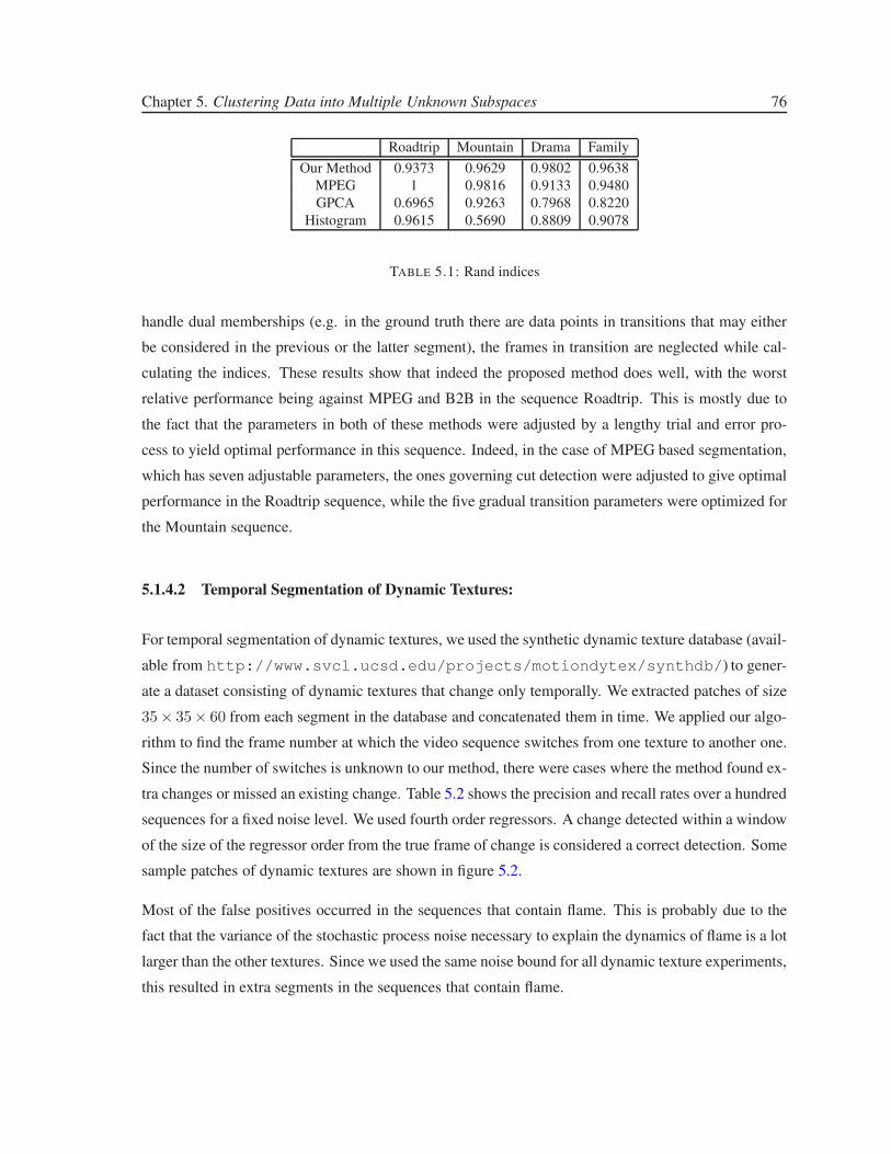
Chapter 5. Clustering Data into Multiple Unknown Subspaces 76
Roadtrip Mountain Drama Family
Our Method 0.9373 0.9629 0.9802 0.9638
MPEG 1 0.9816 0.9133 0.9480
GPCA 0.6965 0.9263 0.7968 0.8220
Histogram 0.9615 0.5690 0.8809 0.9078
TABLE 5.1: Rand indices
handle dual memberships (e.g. in the ground truth there are data points in transitions that may either
be considered in the previous or the latter segment), the frames in transition are neglected while cal-
culating the indices. These results show that indeed the proposed method does well, with the worst
relative performance being against MPEG and B2B in the sequence Roadtrip. This is mostly due to
the fact that the parameters in both of these methods were adjusted by a lengthy trial and error pro-
cess to yield optimal performance in this sequence. Indeed, in the case of MPEG based segmentation,
which has seven adjustable parameters, the ones governing cut detection were adjusted to give optimal
performance in the Roadtrip sequence, while the five gradual transition parameters were optimized for
the Mountain sequence.
5.1.4.2 Temporal Segmentation of Dynamic Textures:
For temporal segmentation of dynamic textures, we used the synthetic dynamic texture database (avail-
able from http://www.svcl.ucsd.edu/projects/motiondytex/synthdb/) to gener-
ate a dataset consisting of dynamic textures that change only temporally. We extracted patches of size
35× 35× 60 from each segment in the database and concatenated them in time. We applied our algo-
rithm to find the frame number at which the video sequence switches from one texture to another one.
Since the number of switches is unknown to our method, there were cases where the method found ex-
tra changes or missed an existing change. Table 5.2 shows the precision and recall rates over a hundred
sequences for a fixed noise level. We used fourth order regressors. A change detected within a window
of the size of the regressor order from the true frame of change is considered a correct detection. Some
sample patches of dynamic textures are shown in figure 5.2.
Most of the false positives occurred in the sequences that contain flame. This is probably due to the
fact that the variance of the stochastic process noise necessary to explain the dynamics of flame is a lot
larger than the other textures. Since we used the same noise bound for all dynamic texture experiments,
this resulted in extra segments in the sequences that contain flame.
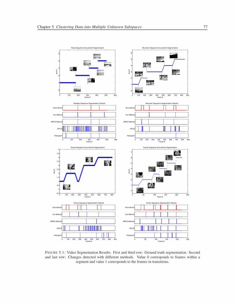
Chapter 5. Clustering Data into Multiple Unknown Subspaces 77
0 100 200 300 400 500 600
0
1
2
3
4
5
Road Sequence Groundtruth Segmentation
frame #
shot #
0 100 200 300 400 500 600 700 800 900
0
1
2
3
4
5
6
Mountain Sequence Groundtruth Segmentation
frame #
shot #
Groundtruth
Roadtrip Sequence Segmentation Results
Our Method
MPEG Method
GPCA
0 100 200 300 400 500 600
Histogram
Frame #
Groundtruth
Mountain Sequence Segmentation Results
Our Method
MPEG Method
GPCA
0 100 200 300 400 500 600 700 800 900
Histogram
Frame #
0 100 200 300 400 500 600 700 800−0.5
0
0.5
1
1.5
2
2.5
3
3.5
4
4.5
5Drama Sequence Groundtruth Segmentation
frame #
shot #
0 50 100 150 200 250
0
1
2
3
4
5
6
7
Family Sequence Groundtruth Segmentation
frame #
shot #
Groundtruth
Drama Sequence Segmentation Results
Our Method
MPEG Method
GPCA
0 100 200 300 400 500 600 700 800 900
Histogram
Frame #
Groundtruth
Family Sequence Segmentation Results
Our Method
MPEG Method
GPCA
0 50 100 150 200 250
Histogram
Frame #
FIGURE 5.1: Video Segmentation Results. First and third row: Ground truth segmentation. Second
and last row: Changes detected with different methods. Value 0 corresponds to frames within a
segment and value 1 corresponds to the frames in transitions.

Chapter 5. Clustering Data into Multiple Unknown Subspaces 78
FIGURE 5.2: Sample dynamic texture patches. From left to right: water, flame, steam.
Sequence Type Precision Recall
Two Different Textures 0.8384 0.9167
Three Different Textures 0.7362 0.6061
TABLE 5.2: Results on Dynamic Texture Database
Next, we consider two more challenging sequences. In the first one, we appended in time one patch
from smoke to another patch from the same texture but transposed. Therefore, both sequences have
the same photometric properties, but differ in the main motion direction: vertical in the first half and
horizontal in the second half of the sequence. For the second example, we generated a sequence of
river by sliding a window both in space and time (by going forward in time in the first half and by
going backward in the second). Hence, dynamics due to river flow are reversed. For these sequences
both histogram and MPEG methods fail to detect the cut since the only change is in the dynamics. On
the other hand, the proposed method correctly segments both sequences. These results are summarized
in Figure 5.3.
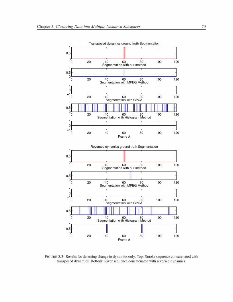
Chapter 5. Clustering Data into Multiple Unknown Subspaces 79
0 20 40 60 80 100 1200
0.5
1Transposed dynamics ground truth Segmentation
0 20 40 60 80 100 1200
0.5
1Segmentation with our method
0 20 40 60 80 100 120−1
0
1Segmentation with MPEG Method
0 20 40 60 80 100 1200
0.5
1Segmentation with GPCA
0 20 40 60 80 100 120−1
0
1Segmentation with Histogram Method
Frame #
0 20 40 60 80 100 1200
0.5
1Reversed dynamics ground truth Segmentation
0 20 40 60 80 100 1200
0.5
1Segmentation with our method
0 20 40 60 80 100 120−1
0
1Segmentation with MPEG Method
0 20 40 60 80 100 1200
0.5
1Segmentation with GPCA
0 20 40 60 80 100 1200
0.5
1Segmentation with Histogram Method
Frame #
FIGURE 5.3: Results for detecting change in dynamics only. Top: Smoke sequence concatenated with
transposed dynamics. Bottom: River sequence concatenated with reversed dynamics.
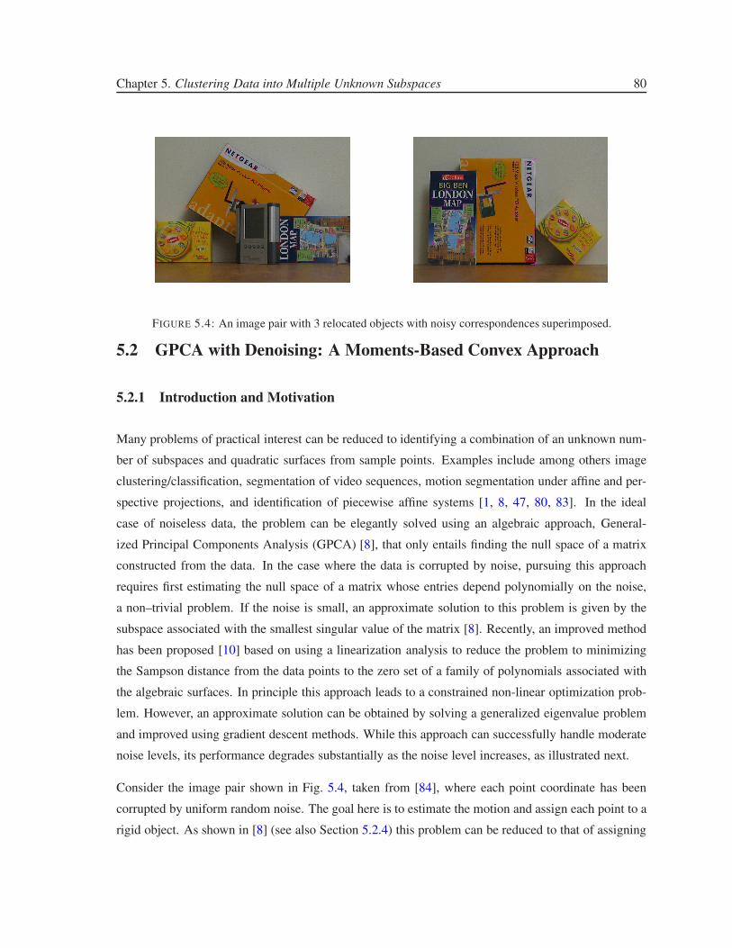
Chapter 5. Clustering Data into Multiple Unknown Subspaces 80
FIGURE 5.4: An image pair with 3 relocated objects with noisy correspondences superimposed.
5.2 GPCA with Denoising: A Moments-Based Convex Approach
5.2.1 Introduction and Motivation
Many problems of practical interest can be reduced to identifying a combination of an unknown num-
ber of subspaces and quadratic surfaces from sample points. Examples include among others image
clustering/classification, segmentation of video sequences, motion segmentation under affine and per-
spective projections, and identification of piecewise affine systems [1, 8, 47, 80, 83]. In the ideal
case of noiseless data, the problem can be elegantly solved using an algebraic approach, General-
ized Principal Components Analysis (GPCA) [8], that only entails finding the null space of a matrix
constructed from the data. In the case where the data is corrupted by noise, pursuing this approach
requires first estimating the null space of a matrix whose entries depend polynomially on the noise,
a non–trivial problem. If the noise is small, an approximate solution to this problem is given by the
subspace associated with the smallest singular value of the matrix [8]. Recently, an improved method
has been proposed [10] based on using a linearization analysis to reduce the problem to minimizing
the Sampson distance from the data points to the zero set of a family of polynomials associated with
the algebraic surfaces. In principle this approach leads to a constrained non-linear optimization prob-
lem. However, an approximate solution can be obtained by solving a generalized eigenvalue problem
and improved using gradient descent methods. While this approach can successfully handle moderate
noise levels, its performance degrades substantially as the noise level increases, as illustrated next.
Consider the image pair shown in Fig. 5.4, taken from [84], where each point coordinate has been
corrupted by uniform random noise. The goal here is to estimate the motion and assign each point to a
rigid object. As shown in [8] (see also Section 5.2.4) this problem can be reduced to that of assigning
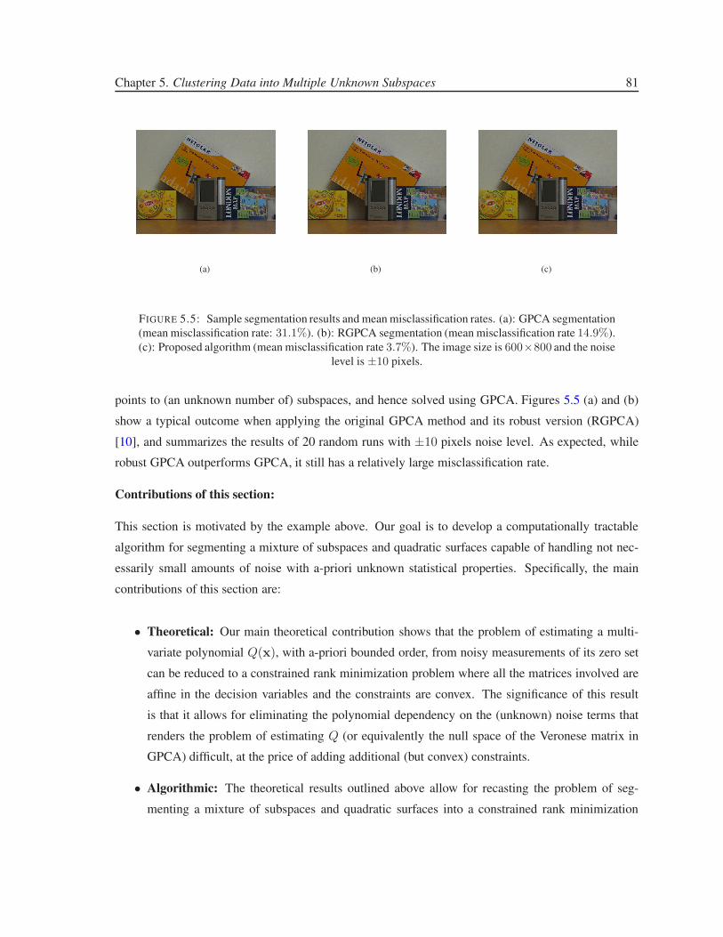
Chapter 5. Clustering Data into Multiple Unknown Subspaces 81
(a) (b) (c)
FIGURE 5.5: Sample segmentation results and mean misclassification rates. (a): GPCA segmentation
(mean misclassification rate: 31.1%). (b): RGPCA segmentation (mean misclassification rate 14.9%).
(c): Proposed algorithm (mean misclassification rate 3.7%). The image size is 600×800 and the noise
level is ±10 pixels.
points to (an unknown number of) subspaces, and hence solved using GPCA. Figures 5.5 (a) and (b)
show a typical outcome when applying the original GPCA method and its robust version (RGPCA)
[10], and summarizes the results of 20 random runs with ±10 pixels noise level. As expected, while
robust GPCA outperforms GPCA, it still has a relatively large misclassification rate.
Contributions of this section:
This section is motivated by the example above. Our goal is to develop a computationally tractable
algorithm for segmenting a mixture of subspaces and quadratic surfaces capable of handling not nec-
essarily small amounts of noise with a-priori unknown statistical properties. Specifically, the main
contributions of this section are:
• Theoretical: Our main theoretical contribution shows that the problem of estimating a multi-
variate polynomial Q(x), with a-priori bounded order, from noisy measurements of its zero set
can be reduced to a constrained rank minimization problem where all the matrices involved are
affine in the decision variables and the constraints are convex. The significance of this result
is that it allows for eliminating the polynomial dependency on the (unknown) noise terms that
renders the problem of estimating Q (or equivalently the null space of the Veronese matrix in
GPCA) difficult, at the price of adding additional (but convex) constraints.
• Algorithmic: The theoretical results outlined above allow for recasting the problem of seg-
menting a mixture of subspaces and quadratic surfaces into a constrained rank minimization

Chapter 5. Clustering Data into Multiple Unknown Subspaces 82
problem. Although in principle rank minimization problems are NP hard, this is a very active
research area in optimization, and in the past few years a number of efficient convex relaxations
have been proposed. Since all matrices involved are affine in the decision variables, the result-
ing overall problem is convex and can be efficiently solved, leading to a tractable segmentation
algorithm. As we illustrate in this section, this algorithm performs well, even in the presence of
substantial noise. An example of this situation is shown in Figure 5.5 (c).
5.2.2 Problem Statement
Let A.= S1∪S2∪ . . . Sn denote an arrangement of subspaces Sk embedded in an ambient space of di-
mension D. To this arrangement of subspaces one can associate a set VnA of homogeneous multivariate
polynomials Qj(x) of degree n that has A as its zero set, that is:
VnA
.= {Qj(x) ∈ Pn : Qj(x) = 0 ⇐⇒ x ∈ A} .
Following [10], in the sequel we will refer to the set VnA as the set of vanishing polynomials of the
arrangement A. Note that each polynomial Qj(x) can be written as Qj = νn(x)T cj , where the vector
cj ∈ Rm, m =
(n+D−1D−1
)
, contains the coefficients of the vanishing polynomial in appropriate order.
It follows that given Np noiseless samples x1, . . . ,xNp ∈ A, the vectors cj span the null space N of
the matrix V(x) =[
νn(x1) νn(x2) . . . νn(xNp)]T
. Thus these vectors (and hence a basis for VnA)
can be found via a simple singular value decomposition of V(x). On the other hand, in the case of
noisy samples xi = xi + ηi the matrix V depends polynomially on the noise ηi. Thus, when ‖η‖ is
not small, the procedure outlined above no longer works, even when replacing the null space N of V
with the subspace associated with its smallest singular values.
Our goal is to develop a computationally tractable algorithm (and the supporting theory) that allows
for estimating both the set of vanishing polynomials and the subspaces from samples corrupted by (not
necessarily small) noise. Specifically, we address the following problem:
Problem 8. [Polynomial estimation and subspace segmentation] Given a (sufficiently dense) set of
noisy samples xi = xi + ηi of points xi drawn from an arrangement of subspaces A, and a–
priori bounds on the number of subspaces, n, and the norm of noise ‖ηi‖2 ≤ ǫ:
1.- Estimate a basis for VnA, the set of vanishing polynomials of A of degree up to n.
2.- Estimate a subspace S⊥k normal to each subspace Sk.
Chapter 5. Clustering Data into Multiple Unknown Subspaces 83
3.- For each noisy sample xi find a subspace Sk, a point xi ∈ Sk and an admissible noise ηi,
‖ηi‖ ≤ ǫ such that xi = xi + ηi.
Our main result establishes that the problem above can be reduced to a constrained rank minimization
problem where all the matrices involved are affine in the optimization variables. Once this result is es-
tablished, tractable algorithms can be obtained by appealing to recently introduced convex relaxations
of rank minimization problems.
5.2.3 Main Results
In this section we present the main theoretical result of the section that allows for recasting Problem
8 into a constrained rank minimization form that can be further relaxed to a convex semi-definite
optimization problem.
Theorem 9. Let {Qj(x)} denote the set of polynomials of an arrangement of subspaces A and denote
by nq its dimension. Consider a set of measurements corrupted by norm-bounded noise
xi = xi + ηi, i = 1, 2 . . . , Np (5.7)
where xi ∈ A and ‖ηi||2 ≤ ǫ. Then:
1. If nq > 1, there exists an admissible noise sequence ηi and Np points xi satisfying (5.7) and
such that Qj(xi) = 0 if and only if there exist Np sequences mi.= {mα} such that the following
conditions hold:
rank{
M(x,m1, . . . ,mNp)}
= h − nq (5.8)
Li(mi) � 0, i = 1, . . . , Np (5.9)
Ki(ǫ,mi) � 0, i = 1, . . . , Np (5.10)
rank(Li(mi)) = 1, i = 1, . . . , Np (5.11)
where h =(
n+D−1D−1
)
; M.= E(V)6 and Li and Ki are the moment matrices, defined in (2.21),
associated with ηi (i.e. the noise affecting the ith sample point).
6Here the expectation operator E acts elementwise on V(x) = V(x − η). That is, M is constructed by replacing all
the monomials in the noise terms η in V(x − η) with the corresponding moments.
Chapter 5. Clustering Data into Multiple Unknown Subspaces 84
2. If nq = 1, e.g. when all the subspaces Sk have dimension D− 1, then the rank constraint (5.11)
is no longer required (e.g only (5.8)-(5.10) need to be enforced.)
Proof. First, if there exits a noise sequence η∗i such that
Qj(xi − η∗i ) = νn(xi − η∗
i )Tcj = 0 for all i, j,
then, the moments mi of the atomic probability measures µi with
Probµi(ηi = η∗
i ) = 1, Probµi(ηi 6= η∗
i ) = 0.
trivially satisfy (5.8) through (5.11) and the vectors cj span the null space of the matrix M(x,m1, . . . ,mNp).
To prove the converse, lets first look at part 1. We start by noting that rank(Li) = 1 is equivalent to the
existence of an unique atomic measure µi with one atom whose moments are equal to mi (see [42])
and, hence, there exist η∗i such that
Probµi(ηi = η∗
i ) = 1, Probµi(ηi 6= η∗
i ) = 0.
Therefore, for this measure, one has
V(x − η∗) = M(x,m1, . . . ,mNp).
Note that (5.10) implies that ‖η∗i ‖2 ≤ ǫ. Given this, let cj be linearly independent vectors which span
the null space of the matrix V(x−η∗). To conclude this part of the proof, define Qj(xi) = νn(xi)Tcj
and xi.= xi − η∗
i . From the reasoning above it follows that
Qj(xi) = νn(xi)T cj = νn(xi − η∗
i )Tcj = 0 for all i, j.
We now turn our attention to part 2. Since condition (5.11) might not be satisfied, the measures µi
compatible with the moment sequences mi are not necessarily atomic measures. However, equa-
tion (5.8) implies that N , the null space of the matrix M(x,m1, . . . ,mNp), has dimension one. Let c
span N , i.e.,
M(x,m1, . . . ,mNp)c = 0.
Chapter 5. Clustering Data into Multiple Unknown Subspaces 85
Linearity of expectation implies that
Eµi[νn(xi − ηi)
T c] = 0.
Therefore, there exist η+i and η−
i within the noise bounds such that
νn(xi − η+i )T c ≥ 0 and νn(xi − η−
i )T c ≤ 0.
Since νn(xi − ηi)T c is a polynomial and, hence, a continuous function of ηi, there exists a η∗
i such
that
νn(xi − η∗i )
T c = 0.
The proof is concluded by defining the unique (up to a multiplying constant) vanishing polynomial
Q(xi) = νn(xi)Tc which, given the reasoning above, satisfies
Q(xi) = νn(xi)Tc = νn(xi − η∗
i )T c = 0 for all i.
Remark 11. Note that, without the rank constraint (5.11), a finite order approximation in (5.9) and (5.10)
only leads to necessary conditions for mi to be moments of a probability distribution. Hence, imple-
menting the approach in part 2 with these truncated matrices only provides an approximation of the
true Q(·). However, the approximation converges to the true solution as the moment approximation
order increases.
5.2.3.1 A Convex Relaxation
Although there are a few methods to solve rank constrained semidefinite programs (see for instance
[85]), these are usually computationally intensive and do not have convergence guarantees. For this
reason, we proceed by relaxing the conditions in order to obtain a convex program that approximates
the original problem and that can be efficiently solved with off–the–shelf solvers. To this end, we first
consider the following problem:
minimizemirank
{
M(x,m1, . . . ,mNp)}
subject to L⌈n
2 ⌉i (mi) � 0 i = 1, . . . , Np
K⌈n
2 ⌉i (ǫ,mi) � i = 1, . . . , Np
(5.12)
Chapter 5. Clustering Data into Multiple Unknown Subspaces 86
where we truncate the moment matrices such that they only contain the moments up to order n (n+1 if
n is odd) which is the maximum order of the noise monomials appearing in the embedded data matrix
V.
Equation (5.12) is an affine matrix rank minimization problem subject to convex constraints. Although
rank minimization is an NP–Hard problem, efficient convex relaxations are available. In particular,
good approximate solutions can be obtained by using a log–det heuristic [51] that relaxes rank mini-
mization to a sequence of convex problems7. Inspired by the adaptive step size defined for weighted
ℓ1 minimization in [65], the following problem is solved at each iteration:
minm1:Np ,Y,Z trace(W(k)y Y) + trace(W
(k)z Z)
subject to
[
Y M(m1:Np)
M(m1:Np)T Z
]
� 0
L⌈n
2 ⌉i (mi) � 0, K
⌈n2 ⌉
i (mi) � 0 i = 1, . . . , Np
(5.13)
where W(k+1)y = (Y(k) + λkI)
−1, W(k+1)z = (Z(k) + λkI)
−1 are weights with Y(k),Z(k) being the
arguments of the optimal solution in the kth iteration; λk, the regularization parameter, is set to the
(h−nq+1)th largest singular value of current optimal M in iteration k; and W(0)y , W
(0)z are initialized
with identity matrices8. Note that the matrices M, L and K are affine in the moment variables mi as
defined in Theorem 9, and Y and Z are symmetric positive definite auxiliary variables. Hence, (5.13)
is a convex semidefinite program.
Remark 12. Although when nq > 1, the relaxation is less tight since we drop the rank–constraints
on the moment matrices, in practice the moment matrices found by solving (5.13) are close to rank
1. Hence approximating them with rank 1 matrices using a singular value decomposition (SVD) gives
satisfactory results (for example see Fig. 5.8).
After solving (5.13), it is possible to extract an admissible noise sequence from the moment matrix L
as described in [87]. In particular, when Li has rank 1, one can retrieve the noise from the elements of
the first singular vector of Li corresponding to first order moments. Once an admissible noise sequence
is obtained, we denoise the data and proceed with segmentation using polynomial differentiation as in
[8].
7Although there are very recent faster algorithms for rank minimization (e.g. [86]), they currently cannot handle semidef-
inite constraints.8The first iteration solves the nuclear norm heuristic. Then each iteration aims to reduce the rank further through the
weighting scheme. In our experiments, the convergence is typically achieved within the first 10 iterations.

Chapter 5. Clustering Data into Multiple Unknown Subspaces 87
5.2.3.2 Extension to Quadratic Surfaces
In this section we briefly present a straightforward extension of our moments-based approach to the
segmentation of a mixture of quadratic surfaces discussed in [1]. In particular, we are interested in
the class of problems that arises in the context of motion segmentation from two perspective views,
given the point correspondences [1, 88, 89]. The main idea is that point correspondences of a single
rigid body satisfy the epipolar constraint xT1 Fx2 = 0 9 where F ∈ R
3×3 is the fundamental matrix and
xj = (xj , yj, 1)T for j = 1, 2, are the corresponding points in two views in homogeneous coordinates.
In the case of n rigid objects, all point correspondences satisfy
n∏
i=1
xT1 Fjx2 = 0. (5.14)
Let z = (x1, y1, x2, y2)T be a joint vector of corresponding pairs and define the perspective embedding
of degree 2n, π2n(z) : R4 → R
m, m =(2+n
n
)2as
π2n(z).=
xα
(1)1
1 yα
(1)2
1 xα
(1)3
2 yα
(1)4
2...
xα
(m)1
1 yα
(m)2
1 xα
(m)3
2 yα
(m)4
2
where the exponents of the monomials satisfy α(k)1 + α
(k)2 ≤ n, α
(k)3 + α
(k)4 ≤ n for all k = 1, . . . ,m.
As in section 5.2.2, we can associate with Eq. (5.14) a polynomial Qj(z) = cTj π2n(z) where cj is
the coefficient vector. It follows that, given Np noiseless corresponding pairs z1, . . . , zNp , the vectors
cj span the null space N of the embedded data matrix P(z) =[
π2n(z1) π2n(z2) . . . π2n(zNp)]T
.
In the noisy case, P(z) depends polynomially on the noise η. However, as before, we can resort to
moments–based rank minimization of E(P) to find a noise sequence η∗ that renders P rank deficient
and obtain its null space (and hence Qj). Once the data is denoised using η∗, we proceed as in [1].
First, we form the mutual contraction subspaces between different pairs (zk, zl) from the derivatives
and hessians of polynomials Qj . Applying spectral clustering to the similarity matrix built from the
subspace angles between mutual contraction subspaces leads then to the desired segmentation.
9As shown in [90], this equation can be written as a quadratic form in the joint image space.
Chapter 5. Clustering Data into Multiple Unknown Subspaces 88
5.2.3.3 Handling Outliers
Upto this point, we assume that the data is only corrupted by norm bounded noise. However, this
assumption could be quite conservative in many real-world problems due to the existence of outliers
that do not belong to any of the algebraic surfaces. One way of eliminating outliers is proposed in
[10] where authors use methods from robust statistics such as influence functions and multivariate
trimming. In this section, we propose a different approach. Namely, we take a step towards handling
outliers in a principled way within our optimization framework. For simplicity of exposition, we
consider the setup in Problem 8 with the addition of outlying data points. The extension to more
general algebraic surfaces follows similar lines.
We call the sample point xj an outlier if the Euclidean distance of xj to the subspace arrangement A
is more than the noise bound ǫ, and an inlier otherwise. The index sets corresponding to inliers and
outliers are denoted by Iin ⊆ {1, . . . , Np} and Iout = {1, . . . , Np} \Iin, respectively. Let Vin be the
matrix whose rows are νn(xi)T for all i ∈ Iin. Then, for all j ∈ Iout and for any noise value ηj with
‖ηj‖2 ≤ ǫ, νn(xj − ηj)T will not be in the row space of Vin. Thus, if we form M as in Theorem
9, M will have some “outlying” rows corresponding to outliers. In order to have a rank deficient
M, we should compensate for the outliers. With this observation in mind, we consider the following
optimization problem:
minm1:Np ,E ‖E‖rs
subject to rank{
M(x,m1, . . . ,mNp) + E}
= h − nq
Li(mi) � 0, i = 1, . . . , Np
Ki(ǫ,mi) � 0, i = 1, . . . , Np
rank(Li(mi)) = 1, i = 1, . . . , Np
(5.15)
where ‖E‖rs counts the number of non-zero rows in E (i.e. row sparsity) and the rest is the same as in
Equations (5.8)-(5.11). Essentially, non-zero rows of E correspond to outlying data points, hence in a
sense (5.15) looks for a compatible model with minimum number of outliers.
As before, we start by relaxing the rank constraints. We drop the rank constraints on Li’s and move
the constraint on M + E to the objective with a Lagrange multiplier:
minimizemi,E rank{
M(x,m1, . . . ,mNp) + E}
+ γ ‖E‖rs
subject to L⌈n
2 ⌉i (mi) � 0 i = 1, . . . , Np
K⌈n
2 ⌉i (ǫ,mi) � i = 1, . . . , Np
(5.16)
Chapter 5. Clustering Data into Multiple Unknown Subspaces 89
Row sparsity is a non-convex function; it is indeed equivalent to sparsity in vector valued sequences
if we treat each row Ei of the matrix E as a vector in the sequence. Hence, the relaxation developed
in Lemma 1 can be applied in this case as well. As for the rank, nuclear norm relaxation can be used.
On top of these relaxations, we adopt the weigthing scheme to obtain following convex program:
minm1:Np ,Y,Z trace(W(k)y Y) + trace(W
(k)z Z) + γ(k)
∑Np
i=1 w(k)i ‖Ei‖∞
subject to
[
Y M(m1:Np) + E
M(m1:Np)T + ET Z
]
� 0
L⌈n
2 ⌉i (mi) � 0, K
⌈n2 ⌉
i (mi) � 0 i = 1, . . . , Np
(5.17)
where W(k+1)y = (Y(k) +λkI)
−1, W(k+1)z = (Z(k) +λkI)
−1, w(k+1)i = 1
∥
∥
∥E(k)i
∥
∥
∥
∞
+δare weights with
Y(k), Z(k) and E(k) being the arguments of the optimal solution in the kth iteration; the regularization
parameter λk is set to the (h − nq + 1)th largest singular value of current optimal M + E in iteration
k; and δ is another small regularization constant. W(0)y , W
(0)z are initialized with identity matrices;
and w(0)i = 1/
√
Np for all i. Lagrange multiplier γ(0) is a tuning parameter that regulates the amount
of outliers. A small value of γ(0) would allow lots of data points to be classified as outliers, whereas a
large value might result in too few outliers preventing the algorithm to find a rank deficient solution.
Once γ(0) is appropriately initialized, γ(k) is set to γ(k) = γ(0)
∥
∥
∥W(k)y
∥
∥
∥
2+∥
∥
∥W(k)z
∥
∥
∥
2
2∥
∥
∥[w
(k)1 ,...,w
(k)Np
]∥
∥
∥
2
so that the effect of
rank minimization term and row sparsity term are approximately constant all through the iterations.
5.2.4 Experiments
In this section we illustrate the ability of the proposed method to deal with relatively large noise using
both synthetic and real data. The data we use here is taken from the literature and thus publicly
available.10
5.2.4.1 Synthetic Data
Example 1: First, we use synthetic data to investigate the performance of the moments–based method
for different number of subspaces, different subspace dimensions and different noise levels. For each
set of examples, we generated 20 random instances of the problem data with data points lying on a
subspace arrangement corrupted by random noise in the direction of subspace normals with uniform
10A reference implementation is provided at http://www.coe.neu.edu/∼necmiye/cvpr10.htm
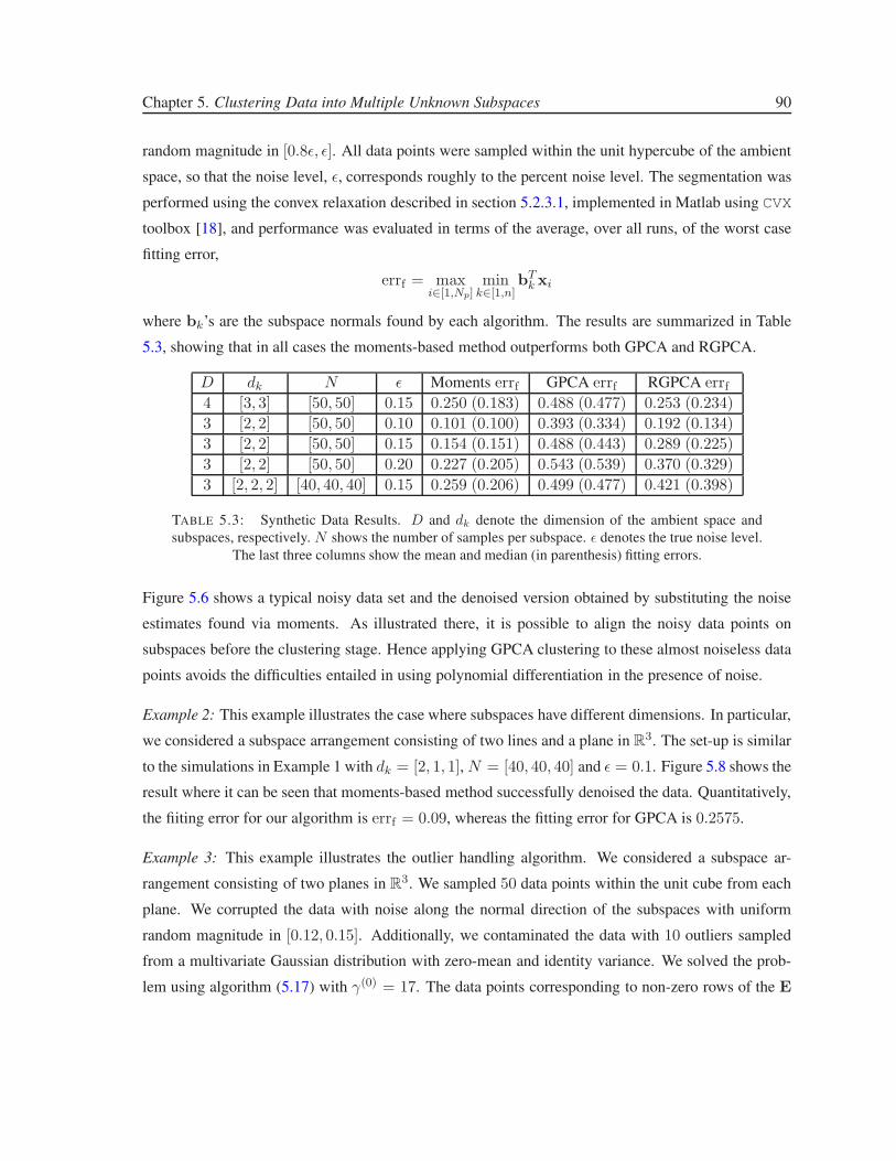
Chapter 5. Clustering Data into Multiple Unknown Subspaces 90
random magnitude in [0.8ǫ, ǫ]. All data points were sampled within the unit hypercube of the ambient
space, so that the noise level, ǫ, corresponds roughly to the percent noise level. The segmentation was
performed using the convex relaxation described in section 5.2.3.1, implemented in Matlab using CVX
toolbox [18], and performance was evaluated in terms of the average, over all runs, of the worst case
fitting error,
errf = maxi∈[1,Np]
mink∈[1,n]
bTk xi
where bk’s are the subspace normals found by each algorithm. The results are summarized in Table
5.3, showing that in all cases the moments-based method outperforms both GPCA and RGPCA.
D dk N ǫ Moments errf GPCA errf RGPCA errf4 [3, 3] [50, 50] 0.15 0.250 (0.183) 0.488 (0.477) 0.253 (0.234)
3 [2, 2] [50, 50] 0.10 0.101 (0.100) 0.393 (0.334) 0.192 (0.134)
3 [2, 2] [50, 50] 0.15 0.154 (0.151) 0.488 (0.443) 0.289 (0.225)
3 [2, 2] [50, 50] 0.20 0.227 (0.205) 0.543 (0.539) 0.370 (0.329)
3 [2, 2, 2] [40, 40, 40] 0.15 0.259 (0.206) 0.499 (0.477) 0.421 (0.398)
TABLE 5.3: Synthetic Data Results. D and dk denote the dimension of the ambient space and
subspaces, respectively. N shows the number of samples per subspace. ǫ denotes the true noise level.
The last three columns show the mean and median (in parenthesis) fitting errors.
Figure 5.6 shows a typical noisy data set and the denoised version obtained by substituting the noise
estimates found via moments. As illustrated there, it is possible to align the noisy data points on
subspaces before the clustering stage. Hence applying GPCA clustering to these almost noiseless data
points avoids the difficulties entailed in using polynomial differentiation in the presence of noise.
Example 2: This example illustrates the case where subspaces have different dimensions. In particular,
we considered a subspace arrangement consisting of two lines and a plane in R3. The set-up is similar
to the simulations in Example 1 with dk = [2, 1, 1], N = [40, 40, 40] and ǫ = 0.1. Figure 5.8 shows the
result where it can be seen that moments-based method successfully denoised the data. Quantitatively,
the fiiting error for our algorithm is errf = 0.09, whereas the fitting error for GPCA is 0.2575.
Example 3: This example illustrates the outlier handling algorithm. We considered a subspace ar-
rangement consisting of two planes in R3. We sampled 50 data points within the unit cube from each
plane. We corrupted the data with noise along the normal direction of the subspaces with uniform
random magnitude in [0.12, 0.15]. Additionally, we contaminated the data with 10 outliers sampled
from a multivariate Gaussian distribution with zero-mean and identity variance. We solved the prob-
lem using algorithm (5.17) with γ(0) = 17. The data points corresponding to non-zero rows of the E
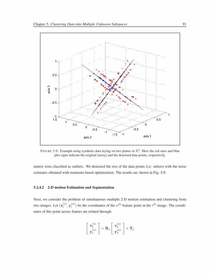
Chapter 5. Clustering Data into Multiple Unknown Subspaces 91
FIGURE 5.6: Example using synthetic data laying on two planes in R3. Here the red stars and blue
plus signs indicate the original (noisy) and the denoised data points, respectively.
matrix were classified as outliers. We denoised the rest of the data points (i.e. inliers) with the noise
estimates obtained with moments-based optimization. The results are shown in Fig. 5.9.
5.2.4.2 2-D motion Estimation and Segmentation
Next, we consider the problem of simultaneous multiple 2-D motion estimation and clustering from
two images. Let (x(n)i ,y
(n)i ) be the coordinates of the nth feature point in the ith image. The coordi-
nates of this point across frames are related through
[
x(n)1
y(n)1
]
= Rj
[
x(n)2
y(n)2
]
+ Tj

Chapter 5. Clustering Data into Multiple Unknown Subspaces 92
0 20 40 60 80 1000
0.05
0.1
0.15
0.2
0.25
0.3
0.35Fitting Errors wrt Subspaces found
moment
gpca
rgpca
true
FIGURE 5.7: Fitting errors for GPCA, RGPCA and moments-based methods for the example in
Fig. 5.6.
where (Rj ,Tj) are the rotation and translation matrices of the motion of the jth object. Rearranging
shows that the vectors, f (n) = [x(n)1 ,y
(n)1 ,x
(n)2 ,y
(n)2 , 1]T corresponding to points belonging to the
same object j lay on a 3 dimensional subspace in R5. If multiple objects with different motions are
present, each lays in a different subspace and thus, in the noiseless case, can be segmented using
GPCA [8].
The image pair shown in Fig. 5.4 is taken from [84]. We manually marked the feature correspondences
and then added uniform random noise to each feature point coordinate in both images. We formed the
vectors f (n), and projected them to R4 using a 5× 4 matrix with orthonormal columns. Note that such
a projection preserves the subspace clusters with probability 1. Specifically, we performed an SVD
of the matrix F = [f (1), . . . , f (N)] = UDVT ) and projected the data using the first 4 columns of U
(i.e.X = UT1:4F). Finally, we applied our method, GPCA and RGPCA to cluster these 4-D vectors
in X. The results, along with a typical segmentation, are summarized in Fig. 5.5, showing that the
moments–based algorithm yields a substantially lower misclassification rate.
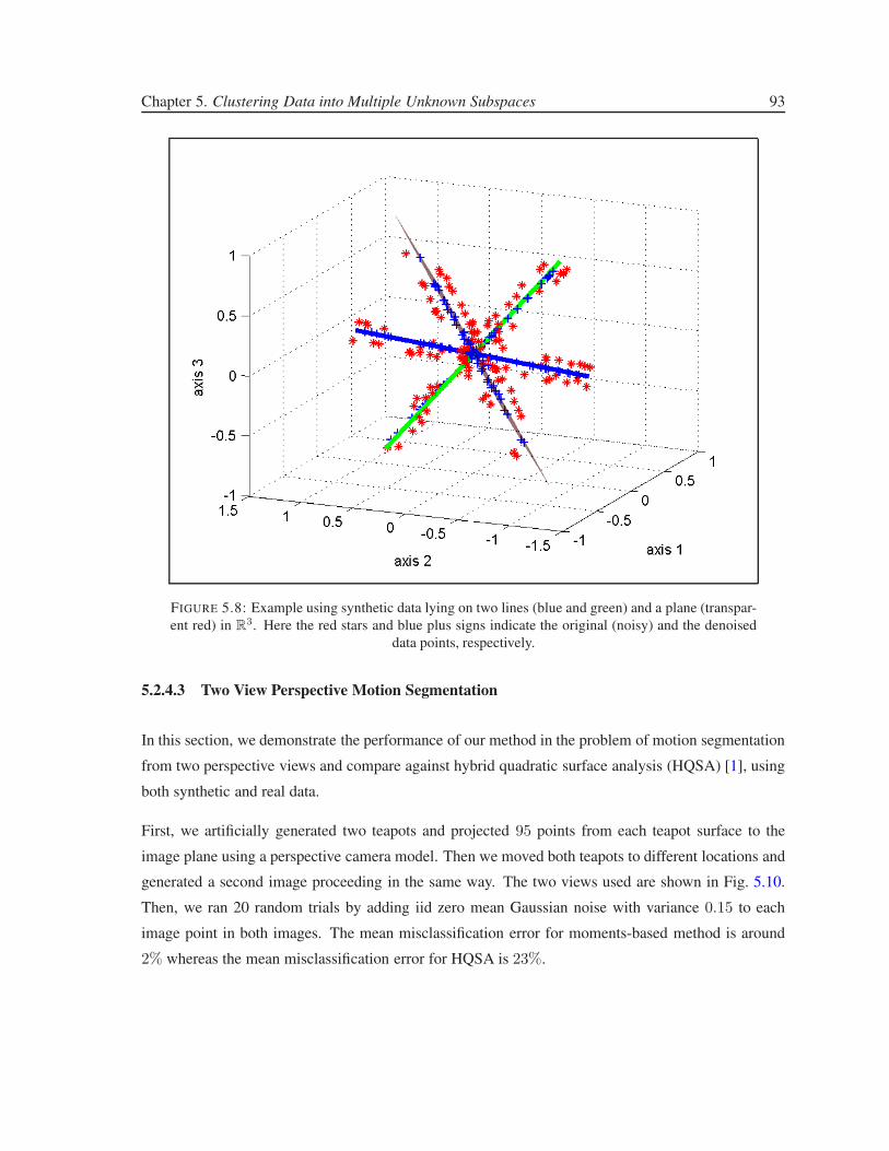
Chapter 5. Clustering Data into Multiple Unknown Subspaces 93
FIGURE 5.8: Example using synthetic data lying on two lines (blue and green) and a plane (transpar-
ent red) in R3. Here the red stars and blue plus signs indicate the original (noisy) and the denoised
data points, respectively.
5.2.4.3 Two View Perspective Motion Segmentation
In this section, we demonstrate the performance of our method in the problem of motion segmentation
from two perspective views and compare against hybrid quadratic surface analysis (HQSA) [1], using
both synthetic and real data.
First, we artificially generated two teapots and projected 95 points from each teapot surface to the
image plane using a perspective camera model. Then we moved both teapots to different locations and
generated a second image proceeding in the same way. The two views used are shown in Fig. 5.10.
Then, we ran 20 random trials by adding iid zero mean Gaussian noise with variance 0.15 to each
image point in both images. The mean misclassification error for moments-based method is around
2% whereas the mean misclassification error for HQSA is 23%.

Chapter 5. Clustering Data into Multiple Unknown Subspaces 94
FIGURE 5.9: Example using synthetic data lying on two planes in R3. Here the red stars and blue plus
signs indicate the original (noisy) and the denoised data points, respectively. Cyan circles indicate the
points identified as outliers.
Next we consider two real examples. Figure 5.11 shows two piles of boxes that are moved in two
different directions. This example is taken from [91]. We used the first and ninth frames of the
sequence as our two perspective views. The missing tracks were ignored. In the resulting segmentation
HQSA misclassifies 29 points whereas the moments-based approach misclassifies only 10 points.
Since our model takes into account only additive noise and this is not the only source of error, the final
classification is not perfect. However, the moments-based approach still outperforms HQSA. For the
next example, we used as perspective views the first and last frames of the “truck2”’ sequence from
the Hopkins 155 dataset [92]. In this case, the misclassification rate for the moments-based approach
is 9.06% (it only misclassifies the left rear wheel as background). On the other hand, HQSA has a
misclassification rate of 42.90%, clustering half of the points on the truck as background.
Sequence Moments-based HQSA
teapot 2.1% 23.42%
boxes 4.05% 11.74%
truck2 9.06% 42.90%
TABLE 5.4: Misclassification rates for perspective motion segmentation examples.
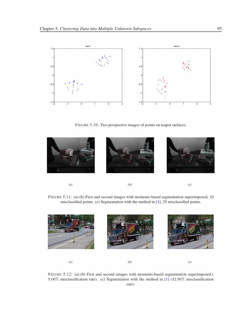
Chapter 5. Clustering Data into Multiple Unknown Subspaces 95
−2 −1 0 1 2 3−1.5
−1
−0.5
0
0.5
1
1.5view 1
−2 −1 0 1 2 3−1.5
−1
−0.5
0
0.5
1
1.5view 2
FIGURE 5.10: Two perspective images of points on teapot surfaces.
(a) (b) (c)
FIGURE 5.11: (a)-(b) First and second images with moments-based segmentation superimposed, 10
misclassified points. (c) Segmentation with the method in [1], 29 misclassified points.
(a) (b) (c)
FIGURE 5.12: (a)-(b) First and second images with moments-based segmentation superimposed (
9.06% misclassification rate). (c) Segmentation with the method in [1] (42.90% misclassification
rate).

Chapter 6
Conclusions and Future Work
We consider the problem of robustly identifying hybrid models from data and minimal a priori as-
sumptions on the model sets and noise level. While this problem is known to be generically NP-hard,
we show that efficient convex relaxations can be obtained by recasting it into an optimization form.
Our main results show that, when an explanation with the minimum number of switches is sought (a
problem relevant for instance in the context of segmentation), the problem can be recast into a sparsi-
fication form and efficiently solved using recently introduced relaxations. A similar idea can be also
used when minimizing the number of submodels. However, in this case, while usually working well in
practice, the sparsification approach is suboptimal. We then consider a related problem when the num-
ber of submodels is known. For this case we develop a moments–based convex optimization approach.
We present parallel results for segmentation of subspace arrangements and more generally algebraic
surfaces. The problem of model (in)validation for switched affine systems is also formulated as an
optimization problem from which it is possible to get convex certificates. The advantages of the pro-
posed techniques over existing methods are illustrated using both simulation examples and non-trivial
problems arising in computer vision. As shown there, while most existing methods perform well in
noiseless scenarios, sparsification–based or moments–based techniques are more robust to noise.
There are some open problems and possible extensions of the proposed methods that have not been
addressed in this dissertation. Future work will include:
• Convergence Analysis: It is important to analyze the convergence properties of proposed iden-
tification schemes. We are currently trying to answer the following questions: “Under what
conditions, does a given algorithm find the true system or segmentation?”; “Is there a noise
96

Chapter 6. Conclusions and Future Work 97
level, below which, the algorithms are guaranteed to converge?”. We have some preliminary
convergence results for the the greedy algorithm for minimum number of switches problem.
Future work will include extending these results to other problems and algorithms.
• Robust Control of Switched Linear Systems: The ultimate goal in system identification is usually
to obtain a model so that one can design controllers. There are some very recent results on
control of switching linear systems [93] and L2 induced norm characterization [94] of such
systems. Another direction for future research is to exploit these results for robust control of
switched linear systems.
• Segmentation of 2-D Images and Arbitrary Graphs: Similar to multidimensional extension in
dynamical case, our results in static case can be extended to perform unsupervised segmentation
of natural or medical images. The idea is to form an uncertain graph with nodes on each pixel
and potential edges connecting each neighboring pixels. Each node can be associated with a
value, which is an invariant of the segments (e.g. this could be the intensity if we presume that
the intensity is almost constant within each segment, or a statistics derived from some local
neighborhood of the pixel) plus an uncertainty. Then each potential edge can be associated
with a weight that is the difference of the values of the two nodes connected by that edge.
Sparsifing the weights of this graph will result in a segmentation with least complex boundary.
We have some preliminary results in this direction where we used the intensity values of the
low frequency components of the images as invariants. The future work will include extending
these result to different frequency scales by identifying relevant invariants and also developing
methods to reduce computational complexity so that it can be applied to larger images/graphs
efficiently.
• Improving Computational Efficiency: Although there are efficient algorithms to solve generic
LPs or SDPs, it is possible to achieve further speed-ups or solve larger-scale problems by using
specially designed optimization algorithms that take into account the specific problem struc-
ture. Such algorithms start appearing both for ℓ1-norm minimization (sparsification) and nu-
clear norm minimization (rank minimization). In this thesis, we just used of-the-shelf convex
programming solvers. In the future, we will incorporate the recently developed fast sparsifi-
cation and rank minimization algorithms (with modifications if necessary) with the methods
proposed in this thesis to further improve computational efficiency.
Appendix A
Sparsity Related Proofs
A.1 Proof of Lemma 1
In order to prove the lemma, we need some preliminary results from convex analysis. For a function
f : C → R, where C ⊆ Rn, the conjugate f⋆ is defined as
f⋆(y) = supx∈C
(〈x, y〉 − f(x))
Under some technical conditions (see [95] Theorem 1.3.5), which are met here, the conjugate of the
conjugate (i.e. f⋆⋆) gives the convex envelope of the function f .
The proof proceeds now along the lines of that of the Theorem 1 in [32], by computing ‖x‖∗∗o , x ∈ S .
The isomorphism I from S to Rd(T−to+1), which simply stacks the elements of the sequence into a
column vector, naturally induces an inner product on S as 〈x, y〉 = 〈I(x),I(y)〉 =∑T
t=1 xT (t)y(t).
For f : S → R, f(x) = ‖x‖0, the conjugate function in C.= ‖x‖∞ ≤ 1 is:
f∗(y) = sup‖x‖∞≤1 {〈x, y〉 − f(x)}
=∑
i∈λ ‖y(i)‖1 − |λ|(A.1)
98
Appendix A. Sparsity Related Proofs 99
where λ = {j : ‖y(j)‖1 > 1, j ∈ {1, 2, . . . , T}} is an index set and |λ| is its cardinality.
f∗∗(z) = supy∈S {〈y, z〉 − f∗(y)}
= supy∈S
{∑
i∈λ y(i)T z(i)
+∑
i/∈λ y(i)T z(i) −∑
i∈λ ‖y(i)‖1 + |λ|}
= supy∈S
{∑
i∈λ y(i)T [z(i) − sign(y(i))]
+∑
i/∈λ y(i)T z(i) + |λ|}
(A.2)
Here we consider two cases:
1) If ‖z‖∞ > 1, it is possible to choose y such that the first term in (A.2) grows unboundedly and
f∗∗(z) → ∞. So the domain of f∗∗ is ‖z‖∞ ≤ 1.
2) If ‖z‖∞ ≤ 1, the first term in the last line of (A.2) is nonpositive. So to maximize the first
term, y(i) values should be chosen small in absolute value for i ∈ λ. Keeping in mind the bounds
imposed on y(i) values by λ, the maximum value of the second term is∑
i/∈λ ‖z(i)‖∞. Similarly,
supy
{∑
i∈λ y(i)T [z(i) − sign(y(i))] + |λ|}
=∑
i∈λ [‖z(i)‖∞ − 1]+ |λ| =∑
i∈λ ‖z(i)‖∞. Hence,
f∗∗(z) =∑T
i=1 ‖z(i)‖∞ .(A.3)
A.2 Proof of Lemma 2
Let g1 = go + h be the solution of the relaxed problem (2.5) and let Io = {t|go(t) 6= 0} be the
indeces of non-zeros elements. From the optimality of g1:
T∑
t=1
||g1(t)||∞ =
T∑
t=1
||go(t) + h(t)||∞ =∑
t∈Io
||go(t) + h(t)||∞ +∑
t/∈Io
||h(t)||∞ ≤T∑
t=1
||go(t)||∞
(A.4)
From the last inequality:
∑
t∈Io||go(t)||∞ −
∑
t∈Io||h(t)||∞ +
∑
t/∈Io||h(t)||∞ ≤
∑Tt=1 ||go(t)||∞
∑
t/∈Io||h(t)||∞ ≤
∑
t∈Io||h(t)||∞
(A.5)
Appendix A. Sparsity Related Proofs 100
Since both g1 and go are feasible, Ah = 0 which implies
AhIo = −AhIco
(A.6)
where hIo(Ico) is the restriction of h to Io(Ic
o , complement of Io). Consider a partition of Ico in to
disjoint sets of cardinality k, Ico = ∪l
j=1Icoj where l ≤ ⌈(T − k)/k⌉. From Eq. (2.6), for all j, we
have:
c1||hIo ± hIcoj||22 ≤ ||AhIo ± AhIc
oj||22 ≤ c2||hIo ± hIc
oj||22 (A.7)
From parallelogram identity:
< AhIo ,AhIcoj
> =||AhIo+AhIc
oj||22−||AhIo−AhIc
oj||22
4
≤c2||hIo+hIc
oj||22−c1||hIo−hIc
oj||22
4
(A.8)
and
− < AhIo ,AhIcoj
> =||AhIo−AhIc
oj||22−||AhIo+AhIc
oj||22
4
≤c2||hIo−hIc
oj||22−c1||hIo+hIc
oj||22
4
=(c2−c1)(||hIo ||
22+||hIc
oj||22)
4
(A.9)
From Eq. (A.6):
||AhIo ||22 = − < AhIo ,AhIc
o> = − < AhIo ,A
∑
j hIcoj
>
= −∑l
j=1 < AhIo ,AhIcoj
>
≤∑l
j=1
(c2−c1)(||hIo ||22+||hIc
oj||22)
4
= c2−c14 (l||hIo ||
22 +
∑lj=1 ||hIc
oj||22)
= c2−c14 (l||hIo ||
22 + ||hIc
o||22)
(A.10)
Now using the norm equivalence identities and eq. (A.5), we have
||hIco||22 =
∑
t∈Ico||h(t)||22
≤∑
t∈Icod||h(t)||2∞
≤ d(
∑
t∈Ico||h(t)||∞
)2
≤ d(∑
t∈Io||h(t)||∞
)2
≤ d(∑
t∈Io||h(t)||2
)2
≤ dk||hIo ||22
(A.11)

Appendix A. Sparsity Related Proofs 101
Following from eq. (A.10):
c1||hIo ||22 ≤ ||AhIo ||
22 ≤ (c2−c1)(l+dk)
4 ||hIo ||22
≤(c2−c1)(⌈T−k
k ⌉+dk)
4 ||hIo ||22
(A.12)
If c1 >(c2−c1)(⌈ T−k
k ⌉+dk)
4 , then we can conclude hIo = 0 which implies hIco
= 0 and g1 = go.
Therefore, a sufficient condition for exactness is:
c1
c2>
T + dk2
T + dk2 + 4k(A.13)
Appendix B
Recovering the Parameters of the Model
in GPCA
Here we recall, for ease of reference, the polynomial differentiation based procedure proposed in [50]
to recover the parameters of the model once cs is computed. The derivative of ps(r) at a point r is
given by
Dps(r) =δps(r)
δr=
s∑
i=1
∏
j 6=i
(bjT r)bi (B.1)
Since biT r = 0 when r is generated by the ith submodel (i.e. σt(r) = i), it follows from (B.1) that
the parameter vector is given by:
bi =Dps(r)
eT Dps(r)
∣
∣
∣
∣
σt(r)=i
(B.2)
where eT = [1, 0, . . . , 0].
Since, in general, the association of data points with submodels σt(r) is unknown, one can use the
following heuristic function, suggested in [8], to choose one point from each submodel {rti}si=1:
rti−1 = argminrt:Dps(rt)6=0
|ps(rt)|‖Dps(rt)‖
+ δ∣
∣(biT rt) · · · (bs
T rt)∣
∣+ δ(B.3)
where δ > 0 is a small number to avoid division by zero in noise free case.
102

Appendix B. Recovering the Parameters of the Model in GPCA 103
Finally, given the parameter vectors {bi}si=1, the mode signal can be computed as follows:
σt = argmini=1,...,s
(biT rt)
2. (B.4)

Bibliography
[1] S. Rao, A. Y. Yang, A. Wagner, and Y. Ma, “Segmentation of hybrid motions via hybrid quadratic
surface analysis,” in ICCV, pp. 2–9, 2005.
[2] R. Alur, C. Belta, F. Ivanicic, V. Kumar, M. Mintz, G. J. Pappas, H. Rubin, and J. Schug, “Hybrid
modeling and simulation of biomolecular networks,” in HSCC, pp. 19–32, 2001.
[3] H. de Jong, J.-L. Gouze, C. Hernandez, M. Page, S. Tewfik, and J. Geiselmann, “Hybrid model-
ing and simulation of genetic regulatory networks: A qualitative approach,” in HSCC, pp. 267–
282, 2003.
[4] A. Bemporad, “Efficient conversion of mixed logical dynamical systems into an equivalent piece-
wise affine form,” Automatic Control, IEEE Transactions on, vol. 49, pp. 832–838, May 2004.
[5] A. Bemporad and M. Morari, “Control of systems integrating logic, dynamics, and constraints,”
Automatica, vol. 35, pp. 407–427, 1999.
[6] D. Pepyne and C. Cassandras, “Optimal control of hybrid systems in manufacturing,” Proceed-
ings of the IEEE, vol. 88, pp. 1108–1123, Jul 2000.
[7] A. Balluchi, L. Benvenuti, M. di Benedetto, C. Pinello, and A. Sangiovanni-Vincentelli, “Au-
tomotive engine control and hybrid systems: challenges and opportunities,” Proceedings of the
IEEE, vol. 88, pp. 888–912, Jul 2000.
[8] R. Vidal, Y. Ma, and S. Sastry, “Generalized principal component analysis (gpca),” IEEE Trans-
actions on Pattern Analysis and Machine Intelligence, vol. 27, pp. 1945–1959, December 2005.
[9] W. Hong, J. Wright, K. Huang, and Y. Ma, “Multiscale hybrid linear models for lossy image
representation,” IEEE Transactions on Image Processing, vol. 15, pp. 3655–3671, December
2006.
104
Bibliography 105
[10] Y. Ma, A. Yang, D. H., and F. R., “Estimation of subspace arrangements with applications in
modeling and segmenting mixed data,” SIAM Review, vol. 50, pp. 413–458, 2008.
[11] J. Ho, M.-H. Yang, J. Lim, K.-C. Lee, and D. J. Kriegman, “Clustering appearances of objects
under varying illumination conditions,” in CVPR (1), pp. 11–18, 2003.
[12] M. Tipping and C. Bishop, “Mixtures of probabilistic principal component analysers,” Neural
Computation, vol. 11, pp. 443–482, 1999.
[13] A. B. Chan and N. Vasconcelos, “Mixtures of dynamic textures,” in IEEE International Confer-
ence on Computer Vision, vol. 1, pp. 641–647, 2005.
[14] O. Rotem, H. Greenspan, and J. Goldberger, “Combining region and edge cues for image seg-
mentation in a probabilistic gaussian mixture framework,” in CVPR07, pp. 1–8, 2007.
[15] S. Boyd and L. Vandenberghe, Convex Optimization. Cambridge Univ. Press, 2004.
[16] J. F. Sturm, “Using sedumi 1.02, a matlab toolbox for optimization over symmetric cones,” 1999.
[17] R. H. Tutuncu, K. C. Toh, and M. J. Todd, “Solving semidefinite-quadratic-linear programs using
sdpt3,” Mathematical Programming Ser. B, vol. 95, pp. 189–217, 2003.
[18] M. Grant and S. Boyd, “CVX: Matlab software for disciplined convex programming.” (web page
and software), June 2009. http://stanford.edu/∼boyd/cvx.
[19] J. Lofberg, “Yalmip : A toolbox for modeling and optimization in MATLAB,” in Proceedings of
the CACSD Conference, 2004.
[20] D. L. Donoho, M. Elad, and V. N. Temlyakov, “Stable recovery of sparse overcomplete repre-
sentations in the presence of noise,” IEEE Transactions on Information Theory, vol. 52, no. 1,
pp. 6–18, 2006.
[21] J. A. Tropp, “Just relax: convex programming methods for identifying sparse signals in noise,”
IEEE Transactions on Information Theory, vol. 52, no. 3, pp. 1030–1051, 2006.
[22] E. J. Candes, J. K. Romberg, and T. Tao, “Stable signal recovery from incomplete and inaccurate
measurements,” Communications on Pure and Applied Mathematics, vol. 59, pp. 1207–1223,
August 2006.
[23] B. K. Natarajan, “Sparse approximate solutions to linear systems,” SIAM Journal on Computing,
vol. 24, no. 2, pp. 227–234, 1995.
Bibliography 106
[24] E. Amaldi and V. Kann, “On the approximability of minimizing nonzero variables or unsatisfied
relations in linear systems,” Theoretical Computer Science, vol. 209, no. 1–2, pp. 237–260, 1998.
[25] J. A. Tropp, “Greed is good: algorithmic results for sparse approximation,” IEEE Transactions
on Information Theory, vol. 50, no. 10, pp. 2231–2242, 2004.
[26] J. A. Tropp and A. C. Gilbert, “Signal recovery from random measurements via orthogonal
matching pursuit,” IEEE Trans. Inform. Theory, vol. 53, pp. 4655–4666, 2007.
[27] D. Needell and R. Vershynin, “Uniform uncertainty principle and signal recovery via regular-
ized orthogonal matching pursuit,” Foundations of Computational Mathematics, vol. 9, no. 3,
pp. 317–334, 2009.
[28] A. M. Bruckstein, D. L. Donoho, and M. Elad, “From sparse solutions of systems of equations
to sparse modeling of signals and images,” SIAM Review, vol. 51, no. 1, pp. 34 – 81, 2009.
[29] Y. Zhang, “On theory of compressive sensing via ℓ1-minimization: Simple derivations and ex-
tensions,” tech. rep., Rice University, 2008.
[30] Y. C. Eldar and M. Mishali, “Robust recovery of signals from a structured union of subspaces,”
Information Theory, IEEE Transactions on, vol. 55, pp. 5302 –5316, nov. 2009.
[31] M. Stojnic, F. Parvaresh, and B. Hassibi, “On the reconstruction of block-sparse signals with an
optimal number of measurements,” Signal Processing, IEEE Transactions on, vol. 57, pp. 3075
–3085, aug. 2009.
[32] M. Fazel, H. Hindi, and S. Boyd, “A rank minimization heuristic with application to minimum
order system approximation,” in American Control Conference, 2001.
[33] M. Fazel, Matrix Rank Minimization with Applications. PhD thesis, Stanford University, 2002.
[34] M. Fazel, H. Hindi, and S. Boyd, “Rank minimization and applications in system theory,” in
American Control Conference, pp. 3273–3278, 2004.
[35] B. Recht, M. Fazel, and P. A. Parrilo, “Guaranteed minimum-rank solutions of linear matrix
equations via nuclear norm minimization.” preprint.
[36] M. Laurent, Emerging Applications of Algebraic Geometry, ch. Sums of squares, moment matri-
ces and optimization over polynomials, pp. 157–270. Springer, 2009.

Bibliography 107
[37] J. A. Shohat and J. D. Tamarkin, The Problem of Moments. Math. Surveys I, Providence, RI:
American Mathematical Society, 1943.
[38] M. G. Krein and A. A. Nudelman, The Markov Moment Problem and Extremal Problems, vol. 50
of Translations of Mathematical Monographs. Providence, RI: American Mathematical Society,
1977.
[39] R. E. Curto and L. A. Fialkow, “Recursiveness, positivity, and truncated moment problems,”
Houston J. Math, vol. 17, pp. 603–635, 1991.
[40] J. L. McGregor, “Solvability criteria for certain n-dimensional moment problems,” Journal of
Approximation Theory, vol. 30, pp. 315–333, 1980.
[41] J. Lasserre, “Global optimization with polynomials and the problem of moments,” SIAM J. Op-
timization, vol. 11, pp. 796–817, 2001.
[42] R. E. Curto and L. A. Fialkow, “Truncated k-moment problems in several variables,” Journal of
Operator Theory, vol. 54, no. 1, pp. 189–226, 2005.
[43] K. Schmudgen, “The k-moment problem for compact semi-algebraic sets,” Mathematische An-
nalen, vol. 289, no. 1, pp. 203–206, 1991.
[44] J. Lasserre, “Convergent sdp-relaxations in polynomial optimization with sparsity,” SIAM J. Op-
timization, vol. 17, no. 3, pp. 822–843, 2006.
[45] H. Waki, S. Kim, M. Kojima, and M. Muramatsu, “Sums of squares and semidefinite program
relaxations for polynomial optimization problems with structured sparsity,” SIAM J. on Opti-
mization, vol. 17, no. 1, pp. 218–242, 2006.
[46] S. Paoletti, A. Juloski, G. Ferrari-Trecate, and R. Vidal, “Identification of hybrid systems: A
tutorial,” European Journal of Control, vol. 13, no. 2, pp. 242–260, 2007.
[47] Y. Ma and R. Vidal, “A closed form solution to the identification of hybrid arx models via the
identification of algebraic varieties,” in Hybrid Systems Computation and Control, pp. 449–465,
March 2005.
[48] A. Bemporad, A. Garulli, S. Paoletti, and A. Vicino, “A bounded-error approach to piecewise
affine system identification,” IEEE Transactions on Automatic Control, vol. 50, no. 10, pp. 1567–
1580, 2005.

Bibliography 108
[49] J. Roll, A. Bemporad, and L. Ljung, “Identification of piesewise affine systems via mixed-integer
programming,” Automatica, vol. 40, pp. 37–50, 2004.
[50] R. Vidal, S. Soatto, Y. Ma, and S. Sastry, “An algebraic geometric approach to the identification
of linear hybrid systems,” in IEEE Conference on Decision and Control, pp. 167–172, Dec. 2003.
[51] M. Fazel, H. Hindi, and S. Boyd, “Log-det heuristic for matrix rank minimization with applica-
tions to hankel and euclidean distance matrices,” in American Control Conference, 2003.
[52] J. Lygeros, K. H. Johansson, S. N. Simic, J. Zhang, and S. S. Sastry, “Dynamical properties of
hybrid automata,” IEEE Transactions on Automatic Control, vol. 48, no. 1, pp. 2–17, 2003.
[53] Z. Qu and P. Perron, “Estimating and testing structural changes in multivariate regressions,”
Econometrica, vol. 75, pp. 459–502, 2007.
[54] J. P. Hespanha, “Uniform stability of switched linear systems: Extensions of lasalle’s invariance
principle,” IEEE Transactions on Automatic Control, vol. 49, no. 4, pp. 470–482, 2004.
[55] A. Gionis and H. Mannila, “Segmentation algorithms for time series and sequence data,” in SIAM
International Conference on Data Mining, 2005. Tutorial.
[56] M. Lobo, M. Fazel, and S. Boyd, “Portfolio optimization with linear and fixed transaction costs,”
Annals of Operations Research, vol. 152, no. 1, pp. 376–394, 2007.
[57] E. J. Candes, M. Wakin, and S. Boyd, “Enhancing sparsity by reweighted l1 minimization,” tech.
rep., California Institute of Technology, 2007.
[58] J. W. Woods, Multidimensional Signal, Image and Video Processing and Coding. Academic
Press, 2006.
[59] R. Vidal, “Identification of spatial-temporal switched arx systems,” in IEEE Conference on De-
cision and Control, pp. 4675–4680, Dec. 2007.
[60] W. M. Rand, “Objective criteria for the evaluation of clustering methods,” Journal of the Ameri-
can Statistical Association, vol. 66, pp. 846–850, 1971.
[61] R. O. Duda, P. E. Hart, and D. G. Stork, Pattern Classification. Wiley & Sons, Inc., second ed.
[62] L. Cooper, J. Liu, and K. Huang, “Spatial segmentation of temporal texture using mixture linear
models,” in Workshop on Dynamical Vision, pp. 142–150, 2005.

Bibliography 109
[63] U. Gargi, R. Kasturi, and S. H. Strayer, “Performance characterization of video-shot-change
detection methods,” IEEE Transactions on Circuits and Systems for Video Technology, vol. 10,
no. 1, pp. 1–13, 2000.
[64] B.-L. Y. and B. Liu, “A unified approach to temporal segmentation of motion jpeg and mpeg
compressed video,” in International Conference on Multimedia Computing and Systems, pp. 81–
88, May 1995.
[65] E. J. Candes, M. Wakin, and S. Boyd, “Enhancing sparsity by reweighted l1 minimization,”
Journal of Fourier Analysis and Applications, vol. 14, no. 5, pp. 877–905, 2008.
[66] N. Ozay, M. Sznaier, C. Lagoa, and O. Camps, “A sparsification approach to set member-
ship identification of a class of affine hybrid systems,” in Proc. 47th IEEE Conf. Dec. Control,
pp. 123–130, 2008.
[67] G. Ferrari-Trecate, M. Muselli, D. Liberati, and M. Morari, “A clustering technique for the iden-
tification of piecewise affine systems,” Automatica, vol. 39, pp. 205–217, 2003.
[68] N. Ozay, C. Lagoa, and M. Sznaier, “Robust identification of switched affine systems via
moments-based convex optimization,” in Proc. 48th IEEE Conf. Dec. Control, pp. 4686–4691,
2009.
[69] C. Feng, C. Lagoa, and M. Sznaier, “Hybrid system identification via sparse polynomial opti-
mization,” in American Control Conference, 2010. (to appear).
[70] K. Poolla, P. Khargonekar, A. Tikku, J. Krause, and K. Nagpal, “A time domain approach to
model validation,” IEEE Transactions on Automatic Control, vol. 39, no. 5, pp. 951–959, 1994.
[71] J. Chen, “Frequency-domain tests for validation of linear fractional uncertain models,” IEEE
Transactions on Automatic Control, vol. 42, pp. 748–760, June 1997.
[72] R. Sanchez Pena and M. Sznaier, Robust Systems Theory and Applications. Wiley & Sons, Inc.,
1998.
[73] M. Sznaier and M. C. Mazzaro, “An lmi approach to control-oriented identification and model
(in) validation of lpv systems,” Automatic Control, IEEE Transactions on, vol. 48, pp. 1619–
1624, sept. 2003.
[74] F. Bianchi and R. Sanchez Pena, “Robust identification/invalidation in an lpv framework,” Inter-
national Journal of Robust and Nonlinear Control, vol. 20, pp. 301–312, Mar. 2009.
Bibliography 110
[75] S. Prajna, “Barrier certificates for nonlinear model validation,” Automatica, vol. 42, no. 1,
pp. 117–126, 2006.
[76] P. A. Parrilo, “Semidefinite programming relaxations for semialgebraic problems,” Mathematical
Programming Ser. B, vol. 96, no. 2, pp. 293–320, 2003.
[77] J. Yuan, H. Wang, L. Xiao, W. Zheng, J. Li, F. Lin, and B. Zhang, “A formal study of shot
boundary detection,” IEEE Transactions on Circuits and Systems for Video Technology, vol. 17,
pp. 168–186, February 2007.
[78] M. Osian and L. Van Gool, “Video shot characterization,” Machine Vision and Applications,
vol. 15, pp. 172–177, July 2004.
[79] N. Petrovic, A. Ivanovic, and N. Jojic, “Recursive estimation of generative models of video,” in
CVPR06, pp. I: 79–86, 2006.
[80] L. Lu and R. Vidal, “Combined central and subspace clustering for computer vision applications,”
in International Conference on Machine Learning, pp. 593–600, 2006.
[81] G. Doretto, A. Chiuso, Y. Wu, and S. Soatto, “Dynamic textures,” IJCV, vol. 51, pp. 91–109,
February 2003.
[82] A. Ghoreyshi and R. Vidal, “Segmenting dynamic textures with ising descriptors, arx models
and level sets,” in WDV06, pp. 127–141, 2006.
[83] J. Ho, M.-H. Yang, J. Lim, K.-C. Lee, and D. J. Kriegman, “Clustering appearances of objects
under varying illumination conditions,” in CVPR (1), pp. 11–18, 2003.
[84] O. Tuzel, R. Subbarao, and P. Meer, “Simultaneous multiple 3d motion estimation via mode
finding on lie groups,” in ICCV, pp. 18–25, 2005.
[85] R. Orsi, U. Helmke, and J. B. Moore, “A newton-like method for solving rank constrained linear
matrix inequalities,” Automatica, vol. 42, pp. 1875–1882, 2006.
[86] J. F. Cai, E. J. Candes, and Z. Shen, “A singular value thresholding algorithm for matrix comple-
tion.” preprint.
[87] D. Henrion and J.-B. Lasserre, Positive Polynomials in Control, ch. Detecting global optimality
and extracting solutions in GloptiPoly, pp. 293–310. Springer, 2005.
Bibliography 111
[88] R. Vidal, Y. Ma, S. Soatto, and S. Sastry, “Two-view multibody structure from motion,” IJCV,
vol. 68, no. 1, pp. 7–25, 2006.
[89] K. Schindler and D. Suter, “Two-view multibody structure-and-motion with outliers through
model selection,” IEEE Trans. Pattern Anal. Mach. Intell., vol. 28, no. 6, pp. 983–995, 2006.
[90] P. Anandan and S. Avidan, “Integrating local affine into global projective images in the joint
image space,” in ECCV (1), pp. 907–921, 2000.
[91] K. Schindler, D. Suter, and H. Wang, “A model selection framework for multibody structure-
and-motion of image sequences,” IJCV, vol. 79, no. 2, pp. 159–177, 2008.
[92] R. Tron and R. Vidal, “A benchmark for the comparison of 3-d motion segmentation algorithms,”
in CVPR, 2007.
[93] F. Blanchini, S. Miani, and F. Mesquine, “A separation principle for linear switching systems and
parametrization of all stabilizing controllers,” Automatic Control, IEEE Transactions on, vol. 54,
pp. 279–292, Feb. 2009.
[94] K. Hirata and J. P. Hespanha, “L2-induced gain analysis for a class of switched systems.” Sub-
mitted to conference publication, Mar. 2009.
[95] J.-B. Hiriart-Urruty and C. Lemarechal, Convex Analysis and Minimization Algortihms II:
Advanced Theory and Bundle Methods, vol. 306 of Grundlehrer der mathematischen Wis-
senschaften. Springer-Verlag, 1993.

Vita
Necmiye Ozay received the B.S. degree in Electrical and Electronics Engineering from Bogazici Uni-
versity, Istanbul in 2004 and the M.S. degree in Electrical Engineering from the Pennsylvania State
University, University Park, PA in 2006. Currently she is a Ph.D. candidate at Electrical and Com-
puter Engineering Department at Northeastern University, Boston, MA. In summer 2008, she was a
research intern at GE Global Research, Niskayuna, NY. She has also held short term visiting positions
at Sabanci University, Istanbul in 2005 and Polytechnic University of Catalunya, Barcelona in 2008.
Her research interests lie at the broad interface of system identification, convex optimization, control
theory, and computer vision. She received the IEEE Control Systems Society Conference on Decision
and Control Best Student Paper Award in 2008 and the IEEE Computer Society Biometrics Workshop
Best Paper Honorable Mention Award in 2009. She is a student member of the IEEE and SIAM.
112
List of Publications
The following list includes all the papers published or submitted for publication by the author during
her graduate studies. Papers denoted by * are directly related to the line of research presented in this
dissertation.
*N. Ozay, M. Sznaier, and C. M. Lagoa, “Model (In)validation of Switched ARX Systems with Un-
known Switches and its Application to Activity Monitoring”, Submitted for conference publication,
March 2010.
*C. Feng, C. M. Lagoa, N. Ozay, and M. Sznaier, “Hybrid System Identification: An SDP Approach”,
Submitted for conference publication, March 2010.
S. Kurugol, N. Ozay, J. G. Dy, G. C. Sharp, and D. Brooks, “Locally Deformable Shape Model
to Improve 3D Level Set based Esophagus Segmentation”, Proc. 20th International Conference on
Pattern Recognition (ICPR), Istanbul, August 2010. (to appear)
*N. Ozay, M. Sznaier, C. M. Lagoa, and O. Camps, “GPCA with Denoising: A Moments-Based
Convex Approach”, Proc. IEEE Conference on Computer Vision and Pattern Recognition (CVPR),
San Francisco, CA, June 2010. (to appear)
*N. Ozay, M. Sznaier, C. M. Lagoa, and O. Camps, “A Sparsification Approach to Set Membership
Identification of Switched Affine Systems”, Submitted for journal publication, May 2009.
*M. Sznaier, O. Camps, N. Ozay, T. Ding, G. Tadmor and D. Brooks, “The role of dynamics in ex-
tracting information sparsely encoded in high dimensional data streams”, in Dynamics of Information
Systems: Theory and Applications (eds. M.J. Hirsch, P.M. Pardalos and R. Murphey), Springer 2010.
113

List of Publications 114
*N. Ozay, C. M. Lagoa, and M. Sznaier,“Robust identification of switched affine systems via moments-
based convex optimization”, Proc. 48th IEEE Conference on Decision and Control (CDC), Shanghai,
P.R. China, December 2009.
N. Ozay, Y. Tong, F. W. Wheeler, and X. Liu, “Improving Face Recognition with a Quality-based
Probabilistic Framework”, Proc. IEEE Computer Society Workshop on Biometrics (in conjunction
with CVPR 2009), pages 134-141, June 2009.
*N. Ozay, M. Sznaier, C. M. Lagoa, and O. Camps, “A Sparsification Approach to Set Membership
Identification of a Class of Affine Hybrid Systems”, Proc. 47th IEEE Conference on Decision and
Control (CDC), pages 123-130, December 2008.
*N. Ozay, M. Sznaier, and O. Camps, “Sequential Sparsification for Change Detection”, Proc. IEEE
Conference on Computer Vision and Pattern Recognition (CVPR), Anchorage, Alaska, June 2008.
N. Ozay, and M. Sznaier, “A Pessimistic Approach to Frequency Domain Model (In)Validation”, Proc.
46th IEEE Conference on Decision and Control (CDC), pages 4895-4900, December 2007.
M. Sznaier, C. M. Lagoa, and N. Ozay, “Risk-adjusted output feedback receding horizon control of
constrained linear parameter varying systems”, International Journal of Robust and Nonlinear Control
(Special issue on Nonlinear Model Predictive Control), 17(17):1614-1633, 2007.
M. Sznaier, C. M. Lagoa, and N. Ozay, “Risk-adjusted output feedback receding horizon control
of constrained linear parameter varying systems”, Proc. European Control Conference (ECC), Kos,
Greece, July 2007.
R. Lublinerman, N. Ozay, D. Zarpalas, and O. Camps, “Activity Recognition from Silhouettes Us-
ing Linear Systems and Model (In)validation Techniques”, Proc. 18th International Conference on
Pattern Recognition (ICPR), pages 347-350, August 2006.