Embed Size (px)
Citation preview
Convex Optimization and Extensions, witha View Toward Large-Scale Problems
Wenbo Gao
Submitted in partial fulfillment of therequirements for the degree of
Doctor of Philosophyunder the Executive Committee
of the Graduate School of Arts and Sciences
COLUMBIA UNIVERSITY
2020

© 2020
Wenbo Gao
All Rights Reserved
Abstract
Convex Optimization and Extensions, with a View Toward
Large-Scale Problems
Wenbo Gao
Machine learning is a major source of interesting optimization problems of current interest.
These problems tend to be challenging because of their enormous scale, which makes it difficult
to apply traditional optimization algorithms. We explore three avenues to designing algorithms
suited to handling these challenges, with a view toward large-scale ML tasks. The first is to
develop better general methods for unconstrained minimization. The second is to tailor methods
to the features of modern systems, namely the availability of distributed computing. The third is
to use specialized algorithms to exploit specific problem structure.
Chapters 2 and 3 focus on improving quasi-Newton methods, a mainstay of unconstrained
optimization. In Chapter 2, we analyze an extension of quasi-Newton methods wherein we use
block updates, which add curvature information to the Hessian approximation on a
higher-dimensional subspace. This defines a family of methods, Block BFGS, that form a
spectrum between the classical BFGS method and Newton’s method, in terms of the amount of
curvature information used. We show that by adding a correction step, the Block BFGS method
inherits the convergence guarantees of BFGS for deterministic problems, most notably a
Q-superlinear convergence rate for strongly convex problems. To explore the tradeoff between
reduced iterations and greater work per iteration of block methods, we present a set of numerical
experiments.
In Chapter 3, we focus on the problem of step size determination. To obviate the need for line
searches, and for pre-computing fixed step sizes, we derive an analytic step size, which we call
curvature-adaptive, for self-concordant functions. This adaptive step size allows us to generalize
the damped Newton method of Nesterov to other iterative methods, including gradient descent
and quasi-Newton methods. We provide simple proofs of convergence, including superlinear
convergence for adaptive BFGS, allowing us to obtain superlinear convergence without line
searches.
In Chapter 4, we move from general algorithms to hardware-influenced algorithms. We consider a
form of distributed stochastic gradient descent that we call Leader SGD, which is inspired by the
Elastic Averaging SGD method. These methods are intended for distributed settings where
communication between machines may be expensive, making it important to set their consensus
mechanism. We show that LSGD avoids an issue with spurious stationary points that affects
EASGD, and provide a convergence analysis of LSGD. In the stochastic strongly convex setting,
LSGD converges at the rate O( 1k) with diminishing step sizes, matching other distributed
methods. We also analyze the impact of varying communication delays, stochasticity in the
selection of the leader points, and under what conditions LSGD may produce better search
directions than the gradient alone.
In Chapter 5, we switch again to focus on algorithms to exploit problem structure. Specifically,
we consider problems where variables satisfy multiaffine constraints, which motivates us to apply
the Alternating Direction Method of Multipliers (ADMM). Problems that can be formulated with
such a structure include representation learning (e.g with dictionaries) and deep learning. We
show that ADMM can be applied directly to multiaffine problems. By extending the theory of
nonconvex ADMM, we prove that ADMM is convergent on multiaffine problems satisfying
certain assumptions, and more broadly, analyze the theoretical properties of ADMM for general
problems, investigating the effect of different types of structure.

Table of Contents
List of Tables . . . . . . . . . . . . . . . . . . . . . . . . . . . . . . . . . . . . . . . . . . vi
List of Figures . . . . . . . . . . . . . . . . . . . . . . . . . . . . . . . . . . . . . . . . . . vii
Acknowledgments . . . . . . . . . . . . . . . . . . . . . . . . . . . . . . . . . . . . . . . . viii
Dedication . . . . . . . . . . . . . . . . . . . . . . . . . . . . . . . . . . . . . . . . . . . . ix
Preface . . . . . . . . . . . . . . . . . . . . . . . . . . . . . . . . . . . . . . . . . . . . . . 1
Chapter 1: Introduction . . . . . . . . . . . . . . . . . . . . . . . . . . . . . . . . . . . . 2
1.1 Improving General Optimization Methods . . . . . . . . . . . . . . . . . . . . . . 5
1.1.1 Curvature in Quasi-Newton methods . . . . . . . . . . . . . . . . . . . . . 6
1.1.2 Step Sizes for Self-Concordant Functions . . . . . . . . . . . . . . . . . . 8
1.2 Making use of Distributed Computing . . . . . . . . . . . . . . . . . . . . . . . . 9
1.3 Algorithms for Structured Problems . . . . . . . . . . . . . . . . . . . . . . . . . 10
Chapter 2: Block BFGS Methods . . . . . . . . . . . . . . . . . . . . . . . . . . . . . . . 12
2.1 Introduction . . . . . . . . . . . . . . . . . . . . . . . . . . . . . . . . . . . . . . 12
2.2 Preliminaries . . . . . . . . . . . . . . . . . . . . . . . . . . . . . . . . . . . . . 15
2.3 Block quasi-Newton Methods . . . . . . . . . . . . . . . . . . . . . . . . . . . . . 16
i

2.3.1 Block BFGS . . . . . . . . . . . . . . . . . . . . . . . . . . . . . . . . . . 16
2.3.2 Rolling Block BFGS . . . . . . . . . . . . . . . . . . . . . . . . . . . . . 20
2.4 Convergence of Block BFGS . . . . . . . . . . . . . . . . . . . . . . . . . . . . . 20
2.5 Superlinear Convergence of Block BFGS . . . . . . . . . . . . . . . . . . . . . . 27
2.6 Modified Block BFGS for Non-Convex Optimization . . . . . . . . . . . . . . . . 41
2.7 Numerical Experiments . . . . . . . . . . . . . . . . . . . . . . . . . . . . . . . . 43
2.7.1 Convex Experiments . . . . . . . . . . . . . . . . . . . . . . . . . . . . . 44
2.7.2 Non-Convex Experiments . . . . . . . . . . . . . . . . . . . . . . . . . . 47
2.8 Concluding Remarks . . . . . . . . . . . . . . . . . . . . . . . . . . . . . . . . . 50
2.9 Supplementary: Details of Experiments . . . . . . . . . . . . . . . . . . . . . . . 50
2.9.1 Logistic Regression Tests (2.7.1) . . . . . . . . . . . . . . . . . . . . . . . 50
2.9.2 Log Barrier QP Tests (2.7.1) . . . . . . . . . . . . . . . . . . . . . . . . . 51
2.9.3 Hyperbolic Tangent Loss Tests (2.7.2) . . . . . . . . . . . . . . . . . . . . 51
Chapter 3: Superlinear Convergence Without Line Searches for Self-Concordant Functions 52
3.1 Introduction . . . . . . . . . . . . . . . . . . . . . . . . . . . . . . . . . . . . . . 52
3.2 Preliminaries . . . . . . . . . . . . . . . . . . . . . . . . . . . . . . . . . . . . . 55
3.3 Self-Concordant Functions . . . . . . . . . . . . . . . . . . . . . . . . . . . . . . 55
3.4 Curvature-Adaptive Step Sizes . . . . . . . . . . . . . . . . . . . . . . . . . . . . 58
3.5 Scaled Gradient Methods . . . . . . . . . . . . . . . . . . . . . . . . . . . . . . . 61
3.5.1 Adaptive Gradient Descent . . . . . . . . . . . . . . . . . . . . . . . . . . 62
3.5.2 Adaptive L-BFGS . . . . . . . . . . . . . . . . . . . . . . . . . . . . . . . 63
3.6 Adaptive BFGS . . . . . . . . . . . . . . . . . . . . . . . . . . . . . . . . . . . . 64
ii

3.6.1 Superlinear Convergence of Adaptive BFGS . . . . . . . . . . . . . . . . . 64
3.7 Hybrid Step Selection . . . . . . . . . . . . . . . . . . . . . . . . . . . . . . . . . 70
3.8 Application to Stochastic Optimization . . . . . . . . . . . . . . . . . . . . . . . . 71
3.9 Numerical Experiments . . . . . . . . . . . . . . . . . . . . . . . . . . . . . . . . 72
3.9.1 Deterministic Methods . . . . . . . . . . . . . . . . . . . . . . . . . . . . 72
3.9.2 Stochastic Methods . . . . . . . . . . . . . . . . . . . . . . . . . . . . . . 78
Chapter 4: Distributed Optimization: The Leader Stochastic Gradient Descent Algorithm . 83
4.1 Introduction . . . . . . . . . . . . . . . . . . . . . . . . . . . . . . . . . . . . . . 83
4.2 Motivating Example: Matrix Factorization . . . . . . . . . . . . . . . . . . . . . . 87
4.3 Definitions and Preliminaries . . . . . . . . . . . . . . . . . . . . . . . . . . . . . 89
4.4 Stationary Points of EASGD . . . . . . . . . . . . . . . . . . . . . . . . . . . . . 91
4.5 Convergence Rates for Stochastic Convex Optimization . . . . . . . . . . . . . . . 92
4.6 Stochastic Convex Optimization with Communication Delay . . . . . . . . . . . . 95
4.7 Stochastic Leader Selection . . . . . . . . . . . . . . . . . . . . . . . . . . . . . . 97
4.8 Nonconvex Optimization . . . . . . . . . . . . . . . . . . . . . . . . . . . . . . . 102
4.9 Quantifiable Improvements of LGD . . . . . . . . . . . . . . . . . . . . . . . . . 103
4.10 A Drawback of LSGD: Implicit Variance Reduction . . . . . . . . . . . . . . . . . 109
Chapter 5: Solving Structured Problems with Multiaffine ADMM . . . . . . . . . . . . . . 112
5.1 Introduction . . . . . . . . . . . . . . . . . . . . . . . . . . . . . . . . . . . . . . 112
5.1.1 Organization of this paper . . . . . . . . . . . . . . . . . . . . . . . . . . 115
5.1.2 Notation and Definitions . . . . . . . . . . . . . . . . . . . . . . . . . . . 115
5.2 Multiaffine Constrained Problems . . . . . . . . . . . . . . . . . . . . . . . . . . 116
iii
5.3 Examples of Applications . . . . . . . . . . . . . . . . . . . . . . . . . . . . . . . 118
5.3.1 Representation Learning . . . . . . . . . . . . . . . . . . . . . . . . . . . 118
5.3.2 Non-Convex Reformulations of Convex Problems . . . . . . . . . . . . . . 119
5.3.3 Max-Cut . . . . . . . . . . . . . . . . . . . . . . . . . . . . . . . . . . . . 120
5.3.4 Risk Parity Portfolio Selection . . . . . . . . . . . . . . . . . . . . . . . . 120
5.3.5 Training Neural Networks . . . . . . . . . . . . . . . . . . . . . . . . . . 121
5.4 Main Results . . . . . . . . . . . . . . . . . . . . . . . . . . . . . . . . . . . . . 122
5.4.1 Assumptions and Main Results . . . . . . . . . . . . . . . . . . . . . . . . 123
5.4.2 Discussion of Assumptions . . . . . . . . . . . . . . . . . . . . . . . . . . 127
5.5 Preliminaries . . . . . . . . . . . . . . . . . . . . . . . . . . . . . . . . . . . . . 133
5.5.1 General Subgradients and First-Order Conditions . . . . . . . . . . . . . . 133
5.5.2 Multiaffine Maps . . . . . . . . . . . . . . . . . . . . . . . . . . . . . . . 135
5.5.3 Smoothness, Convexity, and Coercivity . . . . . . . . . . . . . . . . . . . 139
5.5.4 Distances and Translations . . . . . . . . . . . . . . . . . . . . . . . . . . 140
5.5.5 K-Ł Functions . . . . . . . . . . . . . . . . . . . . . . . . . . . . . . . . . 142
5.6 General Properties of ADMM . . . . . . . . . . . . . . . . . . . . . . . . . . . . . 144
5.6.1 General Objective and Constraints . . . . . . . . . . . . . . . . . . . . . . 144
5.6.2 General Objective and Multiaffine Constraints . . . . . . . . . . . . . . . . 149
5.6.3 Separable Objective and Multiaffine Constraints . . . . . . . . . . . . . . . 154
5.7 Convergence Analysis of Multiaffine ADMM . . . . . . . . . . . . . . . . . . . . 156
5.7.1 Proof of Theorem 5.4.1 . . . . . . . . . . . . . . . . . . . . . . . . . . . . 156
5.7.2 Proof of Theorem 5.4.3 . . . . . . . . . . . . . . . . . . . . . . . . . . . . 162
5.7.3 Proof of Theorem 5.4.5 . . . . . . . . . . . . . . . . . . . . . . . . . . . . 165
iv

5.8 Supplementary: Alternate Deep Neural Net Formulation . . . . . . . . . . . . . . 165
5.9 Supplementary: Formulations with Closed-Form Subproblems . . . . . . . . . . . 166
5.9.1 Representation Learning . . . . . . . . . . . . . . . . . . . . . . . . . . . 166
5.9.2 Risk Parity Portfolio Selection . . . . . . . . . . . . . . . . . . . . . . . . 167
References . . . . . . . . . . . . . . . . . . . . . . . . . . . . . . . . . . . . . . . . . . . . 180
v
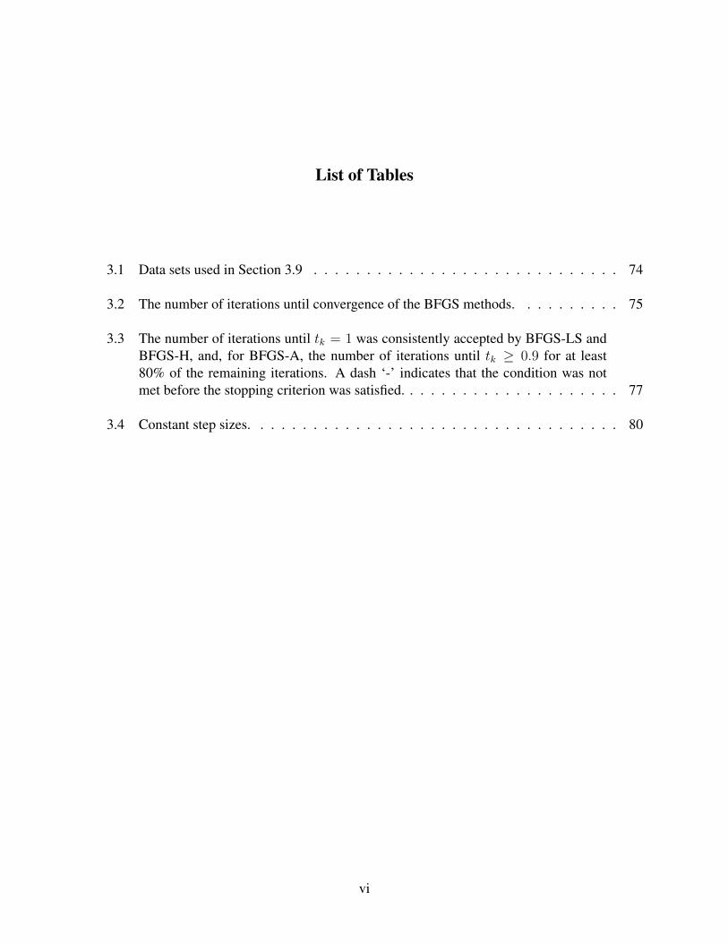
List of Tables
3.1 Data sets used in Section 3.9 . . . . . . . . . . . . . . . . . . . . . . . . . . . . . 74
3.2 The number of iterations until convergence of the BFGS methods. . . . . . . . . . 75
3.3 The number of iterations until tk = 1 was consistently accepted by BFGS-LS andBFGS-H, and, for BFGS-A, the number of iterations until tk ≥ 0.9 for at least80% of the remaining iterations. A dash ‘-’ indicates that the condition was notmet before the stopping criterion was satisfied. . . . . . . . . . . . . . . . . . . . . 77
3.4 Constant step sizes. . . . . . . . . . . . . . . . . . . . . . . . . . . . . . . . . . . 80
vi
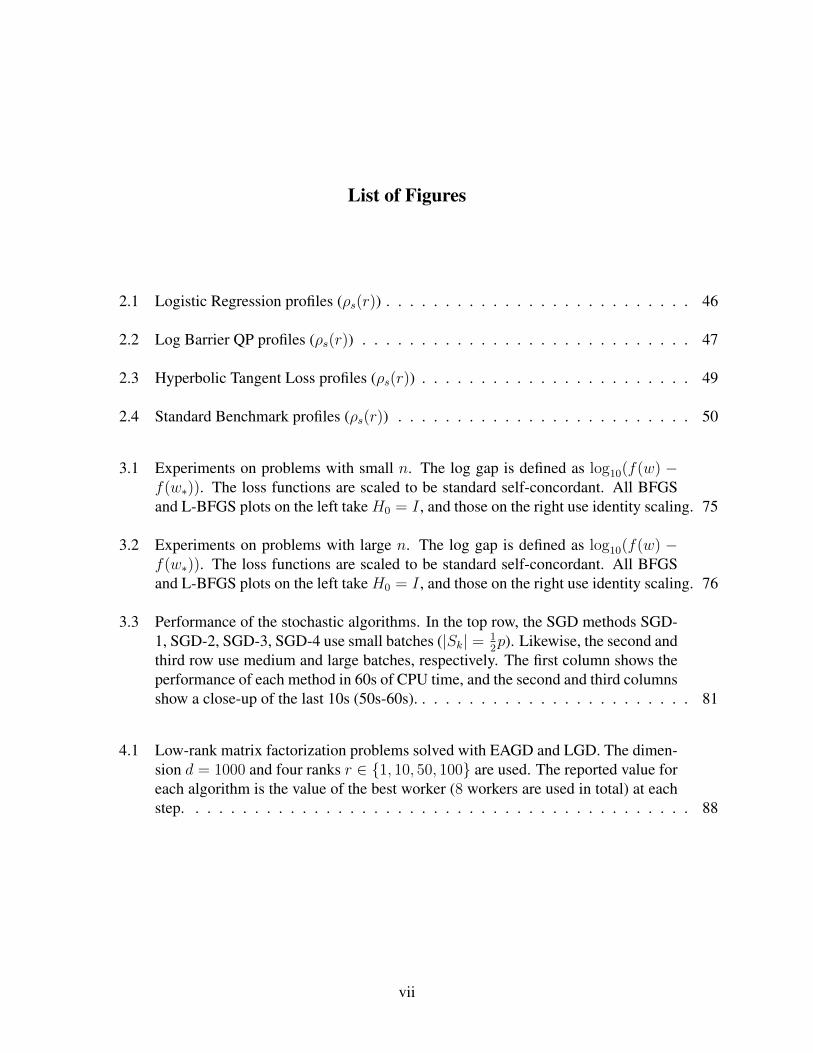
List of Figures
2.1 Logistic Regression profiles (ρs(r)) . . . . . . . . . . . . . . . . . . . . . . . . . . 46
2.2 Log Barrier QP profiles (ρs(r)) . . . . . . . . . . . . . . . . . . . . . . . . . . . . 47
2.3 Hyperbolic Tangent Loss profiles (ρs(r)) . . . . . . . . . . . . . . . . . . . . . . . 49
2.4 Standard Benchmark profiles (ρs(r)) . . . . . . . . . . . . . . . . . . . . . . . . . 50
3.1 Experiments on problems with small n. The log gap is defined as log10(f(w) −f(w∗)). The loss functions are scaled to be standard self-concordant. All BFGSand L-BFGS plots on the left take H0 = I , and those on the right use identity scaling. 75
3.2 Experiments on problems with large n. The log gap is defined as log10(f(w) −f(w∗)). The loss functions are scaled to be standard self-concordant. All BFGSand L-BFGS plots on the left take H0 = I , and those on the right use identity scaling. 76
3.3 Performance of the stochastic algorithms. In the top row, the SGD methods SGD-1, SGD-2, SGD-3, SGD-4 use small batches (|Sk| = 1
2p). Likewise, the second and
third row use medium and large batches, respectively. The first column shows theperformance of each method in 60s of CPU time, and the second and third columnsshow a close-up of the last 10s (50s-60s). . . . . . . . . . . . . . . . . . . . . . . . 81
4.1 Low-rank matrix factorization problems solved with EAGD and LGD. The dimen-sion d = 1000 and four ranks r ∈ 1, 10, 50, 100 are used. The reported value foreach algorithm is the value of the best worker (8 workers are used in total) at eachstep. . . . . . . . . . . . . . . . . . . . . . . . . . . . . . . . . . . . . . . . . . . 88
vii

Acknowledgements
First, my deep gratitude to my advisor, Don Goldfarb. This journey would not have been possible
without his guidance, in research and in life. Don’s work, which has shaped modern optimization,
is an inspiration to me, and I can only hope to be as prolific. I am honored to be his student.
I thank my other collaborators: Frank E. Curtis and Anna Choromanska, for interesting problems
and excellent papers;
Krzysztof Choromanski, for introducing me, with his usual inexhaustible energy, to exciting new
areas of reinforcement learning;
Xingyou Song, Laura Graesser, and Vikas Sindhwani, for fruitful collaborations and great times
during my Google internship.
I thank Dan Bienstock and Shipra Agrawal, for serving on my committee, and for the inspiration
of their work.
I thank the department staff for handling administrative matters. In particular, thanks to Liz
Morales for going above and beyond.
I thank my friends; a better group you could not find. In no particular order: RR, RX, AC, RJ,
MO, FL, CZ, ZQ, EB, FF, SY, GXY, JL, MU, JZ, AZ, KG, MH, RS, SY, YT, MX, BY, and AL.
Finally, my gratitude to my parents, Min Li and Luomin Gao, for supporting me throughout my
life. Nothing would have been possible without you.
viii

To my parents.
ix

Preface
The main chapters of this thesis are closely adapted from published papers:
• Chapter 2 is based on the article Block BFGS Methods [1], SIAM Journal on Optimization
28(2), 2018. This article is joint with Donald Goldfarb.
• Chapter 3 is based on Quasi-Newton Methods: Superlinear Convergence without Line
Searches for Self-Concordant Functions [2], Optimization Methods and Software 34(1),
2018. This article is joint with Donald Goldfarb.
• Chapter 4 is based on Leader Stochastic Gradient Descent for Distributed Training of Deep
Learning Models [3], Advances in Neural Information Processing Systems 32, 2019. This
article is joint with Yunfei Teng, Francois Chalus, Donald Goldfarb, Anna Choromanska,
and Adrian Weller. The results in Chapter 4 are the work of the author.
• Chapter 5 is based on ADMM for Multiaffine Constrained Optimization [4], Optimization
Methods and Software 35(2), 2020. This article is joint with Donald Goldfarb and Frank E.
Curtis.
1

Chapter 1: Introduction
The field of optimization has progressed enormously in the past century. The advent of elec-
tronic computers, and the subsequent rapid growth in computing power, made mathematical mod-
eling and optimization applicable to a vast number of new problems. Though modern methods
are based on the same fundamental principles that date back to the invention of calculus, many
new challenges have arisen as the scale and complexity of optimization problems grows, with ever
more ambitious problems entering the realm of tractability over time. This calls for new advances
in optimization methods, in parallel with improvements in computer hardware.
The predecessors of modern optimization methods have a long history, and arose in the con-
text of solving systems of equations in physics, rather than optimization per se. Gradient descent,
which is now ubiquitous and perhaps the most fundamental method, was described (in an early
form) by Cauchy in his 1847 paper [5] on computing orbits of astronomical bodies. The method
now known as Newton’s method, or the Newton-Raphson method, was developed by Viète [6],
Newton [7, 8] and Raphson [9] as an algorithm for solving nonlinear systems of equations, mo-
tivated again by astronomy (in Newton’s case). Simpson [10] was perhaps the first to explicitly
identify that Newton’s method could be used for function maximization by solving the system
f ′(x) = 0. A detailed survey of the history of Newton’s method is available in [11].
Both gradient descent and Newton’s method continue to be powerful and useful methods. How-
ever, using the basic version of these algorithms on modern problems is often impractical. In recent
years, many optimization problems of interest have originated in machine learning. Without delv-
ing deeply into the statistical origins of machine learning, which is beyond the scope of this thesis,
these problems can often be formulated as:
minxf(x) = Eξ`(x; ξ)
2
where x ∈ Rn is the decision variable, ξ is a random variable that typically represents different
members of an underlying population, and `(x; ξ) is a loss function measuring the performance of
the parameters x on the instance ξ. In practice, the population distribution of ξ is not available, and
we instead perform empirical risk minimization (ERM), minimizing the empirical loss:
minx∈Rn
f(x) =1
N
N∑i=1
`(x; ξi)
where ξ1, . . . , ξN is a set of data points.
The number of parameters (n) is often extremely large. Indeed, the most successful class of ma-
chine learning algorithms, deep learning, make use of heavily over-parameterized models. Break-
throughs in computer vision [12] and natural language processing [13] have used increasingly large
models; the Resnet-1202 network [12] has 19.4 million parameters, and BERT-LARGE [13] has
340 million parameters. Recent experiments show that deep learning often exhibits a ‘double de-
scent’ curve [14], which defies the classical tradeoff between bias and variance. Instead, a new
regime exists when the number of model parameters exceeds the ‘interpolation threshold’; below
the threshold, generalization performance follows the classical U-shaped curve, but then descends
again as the model size grows further. Practitioners often favor larger models, especially in natural
language processing, where state-of-the-art models may have sizes in the range of one to ten billion
parameters (e.g. [15]).
Another challenge arises because the number of data points N is often large, and indeed, must
be for machine learning to be effective. This makes it prohibitively time-consuming to evaluate
the full average 1N
∑Ni=1 `(x; ξi) over all N points, or the average of the gradients. Instead, it
is standard to use a stochastic method, which at each iteration subsamples a minibatch of the
data points and estimates the function or gradient over the minibatch. This algorithm, stochastic
gradient descent (SGD), is the underlying tool that enables machine learning [16, 17]. The use of
minibatches opens up new avenues, from exploiting hardware to most efficiently parallelize over
data, to adapting algorithms to mitigate the additional stochasticity from subsampling.
3
The problems arising from machine learning often have several features which makes it difficult
to directly apply classical optimization algorithms.
1. When the number of parmameters is large, it is impossible to use any implementation of
Newton’s method which stores a dense Hessian matrix. A model with 108 parameters has
roughly 12· 1016 entries1 which requires 10 quadrillion bytes of memory if each entry is
stored as a half-precision floating point number.
2. Loss functions induced by ERM are often highly nonconvex, and even when convex, can
be very ill-conditioned. Gradient descent is known to converge extremely slowly on such
problems.
In this thesis, we focus on three different approaches to enhancing and extending optimization
methods to handle the challenges of large-scale problems. We first introduce the approaches here
and provide a brief summary. In the following sections, we describe each approach in greater
detail, which also serves as an overview of the chapters of this thesis.
Enhanced General Algorithms Gradient descent, BFGS, and Newton’s method are all instances
of general methods for unconstrained optimization problems. That is, they apply to any
problem of the form
minx∈Rn
f(x)
where f is assumed only to be smooth to a sufficient order. Under certain conditions, such
as (strong) convexity, it can be shown that these methods are convergent, and at a particular
rate. In Section 1.1, we focus on quasi-Newton methods, and describe techniques for better
general-purpose quasi-Newton algorithms. The two main aspects we consider are increasing
the use of curvature and better step size selection.
Distributed Computing The performance of sequential algorithms is inherently bounded by phys-
ical limitations on processor speed, which may be approaching [18]. To surpass these limits,
1Assuming we store only the upper triangle of the Hessian.
4

there has been an increased focus on the use of parallel and distributed computing to make
use of widely available computers, which individually may not be very powerful. The strat-
egy of using distributed commodity hardware instead of expensive specialized systems is
often efficient and more practical [19]. However, parallel and distributed algorithms are also
inherently more complicated than sequential algorithms, with the new mechanic of commu-
nication. While there is a straightforward way to parallelize Stochastic Gradient Descent for
machine learning using the data-parallel paradigm, this technique incurs high communica-
tion costs which is ill-suited for computers distributed over a network. In Section 1.2, we
discuss a new distributed SGD method with multiple independent copies of the parameters,
allowing for reduced communication costs.
Structured Problems Problems often belong to classes which have additional structure beyond
the general problem min f(x). An important example is linear programming (LP), where
the objective and constraints consist of linear functions. Extremely efficient specialized algo-
rithms exist for LP which take advantage of the linear structure. The class of ERM problems
can also be considered as a structured class, with algorithms specifically designed to exploit
the finite-sum nature of the objective function to obtain speedups over batch gradient descent
[20, 21, 22].
In Section 1.3, we consider a different class of structured problems, namely those with a sep-
arable structure amenable to the alternating direction method of multipliers (ADMM). Our
interest is in generalizing ADMM to problems where variables are coupled in a multiaffine
fashion, which arises when learning representations from data.
1.1 Improving General Optimization Methods
General optimization methods are those which do not rely on any special properties of the
problem to be solved. As mentioned above, two of the most important examples, which are closely
linked with the history of optimization, are gradient descent and Newton’s method.
5
These methods can be viewed as part of a larger spectrum. Gradient descent is a first-order
method in that it assumes the objective function to be differentiable, and uses only the value of the
objective function (the zero-th order) and the gradient. Newton’s method is a second-order method
which assumes the objective function to be twice differentiable, and uses both the gradient and
the Hessian. Neither method is unambiguously superior to the other across all problems. A trade-
off exists between the convergence rate and the computational expense per step. While gradient
descent can achieve only a sublinear or linear rate of convergence, each step is typically fast to
compute, whereas Newton’s method can achieve (local) quadratic convergence at the expense of
computing the Hessian and solving the Newton system.
Quasi-Newton (QN) methods exist between these two extremes. A QN method maintains an
approximation Bk of the Hessian and generates steps by solving the Newton system using its
Hessian approximation, i.e
xk+1 = xk − λkB−1k ∇f(xk)
The most successful quasi-Newton method is BFGS [23, 24, 25, 26], which uses a particular
updating scheme for the matrices Bk. BFGS itself is part of a spectrum of QN methods known as
the Broyden class [27], which includes BFGS as one endpoint and the DFP method [28, 29] as the
other2. The methods of the Broyden class aim to incorporate information about the true Hessian
action along one dimension into the approximation Bk, using a rank-two update matrix.
There are two main ingredients to improving quasi-Newton methods:
• How can we best make use of curvature information in the matrix Bk?
• How do we select the step sizes λk?
1.1.1 Curvature in Quasi-Newton methods
The idea of increasing the amount of curvature information stored in the Hessian approximation
dates back to Schnabel [30], who considered systems of secant equations. However, this approach
2The DFP method is the first known quasi-Newton method.
6
had technical limitations and received little attention until it was revisited for machine learning
problems in [31]. A major point of divergence in [31], which overcame the technical issues of
[30], was the use of the true Hessian action ∇2f(xk) · sk on the vector sk as opposed to the
gradient difference ∇f(xk + sk) − ∇f(xk). This was proposed in an earlier work on stochastic
L-BFGS for machine learning [32], who noted that using a subsampled stochastic Hessian action
produced better results than differencing subsampled stochastic gradients. It was also noted that
in many machine learning problems, the (subsampled) Hessian-vector product ∇2f(xk) · dk could
be computed in roughly the same time as the subsampled gradient, making it practical to use even
for problems with a large number of parameters. This led to the Stochastic Block L-BFGS method
of [31], which proposed performing BFGS updates with higher-dimensional systems BkDk =
∇2f(xk)Dk, where Dk = [d1 . . . dq] is a column matrix of q directions.
This leads to a new spectrum of QN methods, which we call Block BFGS, with varying amounts
of curvature information, depending on the number q of directions in the update. For q = 1, we
recover a rank-two update similar to the classical BFGS method, whereas q = n is equivalent to
Newton’s method. Intermediate values of q allow us to trade off between using more second-order
information, and having to compute more Hessian-vector products.
While the q = n case is generally equivalent to Newton’s method (it holds if the Hessian andDk
are both nonsingular), the q = 1 case is not equivalent to BFGS. In the original BFGS method, the
gradient difference∇f(xk + dk)−∇f(xk) is guaranteed to have certain useful properties because
of the Armijo-Wolfe line search used to find λk. Replacing it by the Hessian action ∇2f(xk) · dk
does not guarantee the same properties hold. This leaves unanswered the question of whether
Block BFGS, even with q = 1, is convergent, and at what rates.
This is the topic addressed in Chapter 2. We show that with a minor modification to detect de-
generacy of Dk, the Block BFGS method is globally convergent on convex problems, and recovers
the Q-superlinear convergence of BFGS for strongly convex problems. We also perform several
experiments to compare different methods in the Block BFGS family, and explore the tradeoff
between using more curvature, and computational time.
7
1.1.2 Step Sizes for Self-Concordant Functions
Selecting the step size λk is crucial for good performance. Two common strategies are line
searches and constant step sizes. A line search is an algorithm which returns a step λk guaranteed
to satisfy certain conditions; a commonly used type is Armijo-Wolfe line search which has two
conditions (2.2.1) and (2.2.2). In contrast, the constant step size strategy selects a single λ and
fixes λk = λ for all steps.
Both strategies have advantages and drawbacks. Line search is adaptive to the local region
of the objective function, and can take larger steps to speed up convergence when appropriate.
However, it requires additional computation at each step, including multiple evaluations of the
objective function and its gradient at various candidate points. For large-scale problems in machine
learning (large N ), even the evaluations of the loss function are generally too costly, making line
search impractical.
The constant step size approach requires no additional computation during the running of the
algorithm, but instead offloads the effort to the meta-problem of setting the hyperparameter λ.
Moreover, using a constant λ may be inefficient, since the iterates may move between regions of
high and low curvature, for which vastly different step sizes are appropriate. This may result in
convergence speed being degraded.
Our goal is to find an analytic step size which is both computationally efficient and has useful
convergence guarantees. This is the question addressed in Chapter 3. We take a cue from the
damped Newton method of Nesterov [33], which is a globally convergent Newton method for the
class of self-concordant functions. Note that the original Newton method uses λk = 1 and is only
locally convergent, even for strongly convex functions [34]. We extend the step size of the damped
Newton method to a curvature-adaptive step size which can be applied to any iterative optimization
method, including gradient descent and BFGS in particular. Our curvature-adaptive step size has
a simple analytic expression, and requires only a single Hessian-vector product to evaluate. We
show that gradient descent and BFGS retain their convergence guarantees with this step size, and
compare it against other schemes in both the deterministic and stochastic settings.
8
1.2 Making use of Distributed Computing
Making effective use of hardware is essential for good performance. Part of the recent success
of machine learning can be attributed to the rise of hardware acceleration, such as using GPUs [35,
36]. Though originally designed for other applications, these accelerators are optimized for fast
numerical linear algebra, which is also the core operation of deep learning.
The same algorithm may be implemented in different ways, with dramatic differences in real
computing time. Consider for example the basic SGD algorithm, which uses the gradient of the
loss function on a random minibatch of size m. The gradient ∇`(x; ξi) for a particular sample ξi
is independent of that for any other sample ξj , and hence can be parallelized. For systems which
support it, computing the gradients of the samples in parallel yields an almostm-fold speedup over
sequentially computing the gradients. On a device such as a GPU, parallelism exists at multiple
levels, for both speeding up primitive operations such as matrix multiplication, and for parallelizing
over data samples.
This strategy of parallelizing calculations over samples is known as data parallelism, and is
supported by almost all major deep learning frameworks [36]. However, its scalability in terms
of the number of machines is ultimately limited by factors such as the communication cost, and
the reduced generalization of large minibatches, which must be mitigated by other techniques
[37]. Instead, we may consider algorithms which allow for different machines (or workers) to
keep independent copies of the model parameters, and perform local training. Our starting point
for such algorithms is Elastic Averaging SGD (EASGD) [38], which solves a global variable
consensus problem:
minx(1),...,x(p),x
1
p
p∑i=1
Eξ`(x(i); ξ) +ρ
2‖x(i) − x‖2. (1.2.1)
Each of the p workers has its own set of the parameters x(i), and are coupled by the penalty
function ‖x(i) − x‖2. A central machine (or coordinator) maintains x, the consensus variable,
which is responsible for maintaining consistency between the workers.
The EASGD method is powerful, but has several disadvantages in theory and practice which
9
arise from its design. The consensus variable x is a decision variable, which causes the global
objective function (1.2.1) to have spurious stationary points. This is especially apparent when the
underlying loss function f has many symmetries, and the workers are attracted to different local
minima.
In Chapter 4, we consider an alternate scheme called Leader SGD (LSGD), where the consen-
sus variable is no longer a decision variable, but rather is computed from the worker x(1), . . . , x(p)
by estimating the best parameters. We show that LSGD avoids certain pitfalls of EASGD, and
analyze the convergence of EASGD. We show that EASGD matches the convergence rate of other
distributed SGD algorithms, and study its properties under various levels of stochasticity and com-
munication delay.
1.3 Algorithms for Structured Problems
We are interested in problems which are amenable to ADMM. A motivating example is the
separable problem having the form minx∈Rn f(x)+g(x) where f, g are individually straightforward
to minimize, but their sum is not. An instance which arises often in machine learning is the use of
regularization; for instance, we may have
minx∈Rn
1
N
N∑i=1
`(x; ξ) + ‖x‖p.
This type of problem can be solved with the ADMM method, which is specialized for separable
objective functions with linearly constrained variables:
minx,y∈Rn
f(x) + g(y)
s.t. x = y
A comprehensive survey of ADMM and its applications can be found in [39].
Existing work on ADMM has focused on the case of linear constraints. However, variables
are often coupled in more complex ways. When learning representations of data, it is often neces-
10
sary to learn both the set of representatives as well as the actual representation of the given data
corresponding. This is typically a bilinear operation, such as convolution. For example, noisy ob-
servations B can be modeled as the result of applying a convolution A to an underlying signal X ,
and we aim to recover both the convolutional kernel and the signal given access to the observation.
The variables then satisfy the relation A ∗ X = Y , where ∗ denotes a convolution. While this
constraint alone makes it ill-posed to recover A and X , sparsity assumptions on X make this a
well-defined optimization problem. Observe that when A is fixed, the resulting equation becomes
linear in X , and likewise for A when X is fixed. This suggests that ADMM may be applicable to
solving this problem.
In Chapter 5, we investigate the properties of ADMM for problems where the constraints are
multiaffine. For such problems, ADMM can be applied in the same way as for linearly-constrained
problems, since the subproblems have the same structure when minimizing for each variable in
turn. We show that under similar assumptions as those used for the analysis of linearly-constrained
nonconvex ADMM, we obtain convergence of ADMM when applied to multiaffine problems, and
present examples of problems with a multiaffine structure.
11

Chapter 2: Block BFGS Methods
2.1 Introduction
The classical BFGS method [23, 24, 26, 25] is perhaps the best known quasi-Newton method
for minimizing an unconstrained function f(x). These methods iteratively proceed along search
directions dk = −B−1k ∇f(xk), where Bk is an approximation to the Hessian ∇2f(xk) at the
current iterate xk. Quasi-Newton methods differ primarily in the manner in which they update
the approximation Bk. The BFGS method constructs an update Bk+1 that is the nearest matrix to
Bk (in a variable metric) satisfying the secant equation Bk+1(xk+1 − xk) = ∇f(xk+1)−∇f(xk)
[23]. This can be interpreted as modifying Bk to act like∇2f(x) along the step xk+1 − xk, so that
successive updates induce Bk to resemble ∇2f(x) along the search directions.
A natural extension of the classical BFGS method is to incorporate information about ∇2f(x)
along multiple directions in each update. This further improves the accuracy of the local Hessian
approximation, allowing one to obtain better search directions. Early work in this area includes
the development by Schnabel [30] of quasi-Newton methods that satisfy multiple (say, q) secant
equations Bk+1s(i)k = ∇f(xk+1)−∇f(xk+1− s(i)
k ) for directions s(1)k , . . . , s
(q)k . This approach has
the disadvantage that the resulting update is generally not symmetric, and considerable modifica-
tions are required to ensure Bk remains positive definite. Consequently, there appears to have been
little interest in quasi-Newton methods with block updates in the years following Schnabel’s initial
report.
More recently, a stochastic quasi-Newton method with block updates was introduced by Gower,
Goldfarb, and Richtárik [31]. Their approach constructs an update which satisfies sketching equa-
tions of the form
Bk+1s(i)k = ∇2f(xk+1)s
(i)k
12

for multiple directions s(i)k . By using sketching equations instead of secant equations, the update
is guaranteed to remain symmetric, and in the case where f(x) is convex, positive definite. The
sketching equations can be thought of as ‘tangent’ equations that requireBk+1 to incorporate infor-
mation about the Hessian∇2f(xk+1) at the most recent point xk+1, as opposed to information about
the average of∇2f(x) between two points, i.e, along a secant. Consequently, in terms of the infor-
mation used, the block updating formula is Newton-like rather than secant-like. A Hessian-vector
product ∇2f(xk+1)s(i)k can generally be computed much faster than the full Hessian ∇2f(xk+1),
and the operation of computing ∇2f(xk+1)s(i)k for multiple directions s(1)
k , . . . , s(q)k can be done in
parallel.
Computing the Hessian-vector products∇2f(xk+1)s(i)k , referred to as Hessian actions, involves
additional work beyond that of classical BFGS updates, where the gradients can be reused to com-
pute ∇f(xk+1)−∇f(xk). However, the increased cost of block updates may be justified in order
to obtain better search directions, for the same reason that Newton’s method often outperforms
gradient descent: the greater cost per iteration is compensated by convergence in fewer iterations,
in regions where the curvature can be used effectively. Our numerical experiments in Section 7
explored this trade-off, and we found that using block updates did result in performance gains on
many problems.
Other experiments indicate that quasi-Newton methods using Hessian actions and block up-
dates are promising for empirical risk minimization problems arising from machine learning.
Byrd, Hansen, Nocedal, and Yuan [32] proposed a stochastic limited-memory algorithm Stochas-
tic Quasi-Newton (SQN), in which the secant equation is replaced by a sub-sampled sketching
equation Bk+1sk = ∇2f(xk+1)sk (here ∇2f(x) denotes a sub-sampled Hessian). The authors
[32] remark that using the sub-sampled Hessian action avoids harmful effects from gradient dif-
ferencing in the stochastic setting. In [31], a stochastic limited-memory method Stochastic Block
L-BFGS, using block updates, outperformed other state-of-the-art methods when applied to large-
scale logistic regression problems.
In this paper, we introduce a deterministic quasi-Newton method Block BFGS. The key fea-
13
ture of Block BFGS is the inclusion of information about ∇2f(x) along multiple directions, by
enforcing that Bk+1 satisfies the sketching equations for a subset of previous search directions. We
show that this method, performed with inexact Armijo-Wolfe line searches, has the same conver-
gence properties as the classical BFGS method. Namely, if f is twice differentiable, convex, and
bounded below, and the gradient of f is Lipschitz continuous, then Block BFGS converges. If,
in addition, f is strongly convex and the Hessian of f is Lipschitz continuous, then Block BFGS
achieves Q-superlinear convergence. Note that we use a slightly modified notion of Q-superlinear
convergence: we prove that the sequence of quotients ‖x(i+1)k − x∗‖/‖x(i)
k − x∗‖, with possibly a
small number of terms removed, converges to 0. The precise statement of this result is given in
Theorem 2.5.1. We also note that our convergence results can easily be extended to block versions
of the restricted Broyden class of quasi-Newton methods as in [27].
These results fill a gap in the theory of quasi-Newton methods, as updates based on the Hessian
action have previously only been used within limited-memory methods, for which the analysis is
significantly simpler. Because of its limited-memory nature, the Stochastic Block L-BFGS method
in [31] is only proved to be R-linearly convergent (in expectation, when using a fixed step size).
For this method, as is the case for the deterministic L-BFGS method [40], the convergence rate
that is proved is worse than the rate for gradient descent (GD), even though in practice, L-BFGS
almost always converges far more rapidly than GD. We believe that our proof of the Q-superlinear
convergence of Block BFGS in this paper provides a rationale for the superior performance of the
Stochastic Block L-BFGS method, and behavior of deterministic limited-memory Block BFGS
methods as well.
Block BFGS can also be applied to non-convex functions. We show that if f has bounded
Hessian, then Block BFGS converges to a stationary point of f . Modified forms of the classical
BFGS method also have natural extensions to block updates, so modified block quasi-Newton
methods are applicable in the non-convex setting.
The paper is organized as follows. Section 2.2 contains preliminaries and describes Armijo-
Wolfe inexact line searches. In Section 2.3, we formally define the Block BFGS method and several
14

variants. In Section 2.4 and Section 2.5 respectively, we show that Block BFGS converges, and
converges superlinearly, for f satisfying appropriate conditions. In Section 2.6, we show that Block
BFGS converges for suitable non-convex functions, and describe several other modifications to
adapt Block BFGS for non-convex optimization. In Section 2.7, we present the results of numerical
experiments for several classes of convex and non-convex problems.
2.2 Preliminaries
The following notation will be used. The objective function of n variables is denoted by f :
Rn → R. We write g(x) for the gradient∇f(x) and G(x) for the Hessian∇2f(x). For a sequence
xk, fk = f(xk) and gk = g(xk). However, we deliberately use Gk = G(xk+1) to simplify the
update formula.
The norm ‖ · ‖ denotes the L2 norm, or for matrices, the L2 operator norm. The Frobenius
norm will be explicitly indicated as ‖ · ‖F . Angle brackets 〈·, ·〉 denote the standard inner product
〈x, y〉 = yTx and the trace inner product 〈X, Y 〉 = Tr(Y TX). We use either notation 〈x, y〉 or yTx
as is convenient. The symbol Σn denotes the space of n × n symmetric matrices, and denotes
the Löwner partial order; hence A 0 means A is positive definite.
An LΣLT decomposition is a factorization of a positive definite matrix into a product LΣLT ,
where L is lower triangular with ones on the diagonal, and Σ = Diag(σ21, . . . , σ
2n). This is com-
monly called an LDLT decomposition in the literature, but we write Σ in place of D as we use D
to denote a matrix whose columns are previous search directions.
In the pseudocode for our algorithm, size(A, 1) and size(A, 2) denote the number of rows
and columns of a matrix A respectively. The ij-entry of a matrix A will be denoted by Aij . We
use Col(A) to denote the linear space spanned by the columns of A. By convention, a sum over an
empty index set is equal to 0.
Our inexact line search selects step sizes λk satisfying the Armijo-Wolfe conditions: for param-
15

eters α, β with 0 < α < 12
and α < β < 1, the step satisfies
f(xk + λkdk) ≤ f(xk) + αλk〈gk, dk〉 (2.2.1)
〈g(xk + λkdk), dk〉 ≥ β〈gk, dk〉. (2.2.2)
Furthermore, our line search always selects λk = 1 whenever this step size is admissible. This is
important in the analysis of superlinear convergence in Section 2.5.
2.3 Block quasi-Newton Methods
In this section, we introduce Block BFGS, a quasi-Newton method with block updates, and
several variants.
2.3.1 Block BFGS
Algorithm 1 Block BFGS
input: x(1)1 , B1, q
1: for k = 1, 2, 3 . . . do2: for i = 1, . . . , q do3: d
(i)k ← −B
−1k g
(i)k
4: λ(i)k ← LINESEARCH(x
(i)k , d
(i)k )
5: s(i)k ← λ
(i)k d
(i)k
6: x(i+1)k ← x
(i)k + s
(i)k
7: end for8: Gk ← G(x
(q+1)k )
9: Sk ← [s(1)k . . . s
(q)k ]
10: Dk ← FILTERSTEPS(Sk, Gk)11: if Dk is not empty then12: Bk+1 ← Bk −BkDk(D
TkBkDk)
−1DTkBk +GkDk(D
TkGkDk)
−1DTkGk
13: else14: Bk+1 ← Bk
15: end if16: x
(1)k+1 ← x
(q+1)k
17: end for
16

Algorithm 2 FILTERSTEPS
input: Sk, Gk output: Dk parameters: threshold τ > 01: Initialize Dk ← Sk, i← 12: while i ≤ size(Dk, 2) do3: σ2
i ← [DTkGkDk]ii −
∑i−1j=1 L
2ijΣjj
4: si ← column i of Dk
5: if σ2i ≥ τ‖si‖2 then
6: Σii ← σ2i
7: Lii ← 18: for j = i+ 1, . . . ,size(Dk, 2) do9: Lji ← 1
Σii([DT
kGkDk]ji −∑i−1
k=1 LikLjkΣkk)10: end for11: i← i+ 112: else13: Delete column i from Dk and row i from L14: end if15: end while
Block BFGS (Algorithm 1) takes q steps in each block, using a fixed Hessian approximation
Bk. We may also take a varying number of steps, bounded above by q, but we assume every
block contains q steps to simplify the presentation. We use a subscript k for the block index, and
superscripts (i) for the steps within each block. The k-th block contains the iterates x(1)k , . . . , x
(q+1)k ,
and x(1)k+1 = x
(q+1)k . At each point x(i)
k , the step direction is d(i)k = −B−1
k g(i)k , and line search is
performed to obtain a step size λ(i)k . We take a step s(i)
k = λ(i)k d
(i)k . The angle between s(i)
k and−g(i)k
is denoted θ(i)k . As Bk is positive definite, θ(i)
k ∈ [0, π2).
After taking q steps, the matrix Bk is updated. Let Gk = G(x(q+1)k ) denote the Hessian at
the final iterate, and form the matrix Sk = [s(1)k . . . s
(q)k ]. We apply the FILTERSTEPS procedure
(Algorithm 2) to Sk, which returns a subset Dk of the columns of Sk satisfying σ2i ≥ τ‖si‖2,
where si is the i-th column of Dk and σ2i is the i-th diagonal entry of the LΣLT decomposition
of DTkGkDk. τ > 0 is a parameter which controls the strictness of the filtering; a small value of
τ permits Dk to contain steps that are closer to being linearly dependent, as well as steps with
smaller curvature. In essence, FILTERSTEPS iteratively computes the LΣLT decomposition of
STk GkSk and discards columns of Sk corresponding to small diagonal entries, with the remaining
columns forming Dk.
17
Define qk to be the number of columns of Dk. If Dk is the empty matrix (all columns were
removed), then no update is performed and Bk+1 = Bk. If Dk is not empty, the matrix Bk is
updated to have the same action as the Hessian Gk on the column space of Dk, or equivalently,
Bk+1Dk = GkDk. (2.3.1)
Let D = Dk, G = Gk. The formula for the update is given by
Bk+1 = Bk −BkD(DTBkD)−1DTBk +GD(DTGD)−1DTG. (2.3.2)
This formula is invariant under a change of basis of Col(Dk), so we can choose Dk to be any
matrix with the same column space. To see this, observe that a change of basis is given by DkP
for an invertible q × q matrix P . The update (2.3.2) for the matrix DkP is given by
Bk+1 = Bk −BkDP (P TDTBkDP )−1P TDTBk +GDP (P TDTGDP )−1P TDTG
= Bk −BkD(DTBkD)−1DTBk +GD(DTGD)−1DTG.
On the other hand, the matrix Dk obtained from filtering Sk is not invariant under a change of
basis of Sk, and it is possible to control the number of columns removed by selecting an appro-
priate basis for Sk. We chose to take Sk = [s(1)k . . . s
(q)k ] in order to retain control over the ratio
det(DTkGkDk)/ det(DT
kBkDk), which is crucial for our theoretical analysis. We also note that in
[31], two other choices for the columns ofDk were studied for use in the Stochastic Block L-BFGS
method, and the results reported there showed that the choice Dk = [s(1)k . . . s
(q)k ] worked best.
As is the case for standard quasi-Newton updates, there are many possible updates that satisfy
equation (2.3.1). The specific Block BFGS update (2.3.2) is derived as follows. Let Hk = B−1k be
the approximation of the inverse Hessian. In contrast with the classical BFGS update, the update
(2.3.2) is chosen so that Hk+1 is the nearest matrix to Hk in a weighted norm, satisfying the system
of sketching equations Hk+1GkDk = Dk rather than a set of secant equations. That is, Hk+1 is the
18
solution to the minimization problem
minH∈Rn×n
‖H −Hk‖Gk
s.t H = HT , HGkDk = Dk
(2.3.3)
where ‖ · ‖Gkis the norm ‖X‖Gk
= Tr(XGkXTGk). This norm is induced by an inner product,
so Hk+1 is an orthogonal projection onto the subspace H ∈ Σn : HGkDk = Dk. In analogy
with the classical BFGS update, Hk+1 has a simple formula in terms of block updates, which was
obtained in [30].
Theorem 2.3.1. The Block BFGS update of Hk is given by
Hk+1 = D(DTGD)−1DT + (I −D(DTGD)−1DTG)Hk(I −GD(DTGD)−1DT ). (2.3.4)
Taking the inverse yields formula (2.3.2). Moreover, as shown in [30], we have
Lemma 2.3.2. If Bk (Hk) and DTkGkDk are positive definite, then the Block BFGS update (2.3.2)
for Bk+1 ((2.3.4) for Hk+1) is positive definite.
Proof. Our proof is adapted from Theorem 3.1 of [30]. Let z ∈ Rn, and define w = DTk z, v =
z −GkDk(DTkGkDk)
−1w. Using formula (2.3.4), we find that
zTHk+1z = wT (DTkGkDk)
−1w + vTHkv
so zTHk+1z ≥ 0. Furthermore, zTHk+1z = 0 only if both w = 0 and v = 0, in which case z = 0.
Hence Hk+1 is positive definite.
In Section 2.4, we show that Block BFGS converges even if Bk = Bk+1 = . . . is stationary. In
Section 2.5, we show that when f is strongly convex, the parameter τ can be naturally chosen so
an update is always performed, and the convergence is superlinear.
In theory, FILTERSTEPS is required to ensure that the update (2.3.2) exists. However, in prac-
tice, one is unlikely to encounter linearly dependent directions, or directions lying exactly in the
19

null space of Gk. Thus, one may omit FILTERSTEPS unless there is reason to believe that Gk is
singular and problems will arise. However, filtering may improve numerical stability, by removing
nearly linearly dependent steps from Dk.
2.3.2 Rolling Block BFGS
Block BFGS uses the same matrix Bk throughout each block of q steps. We could also add
information from these steps immediately, at the cost of doing far more updates. This variant,
Rolling Block BFGS, performs a block update after every step, using a subset Dk of the previous
q steps. Dk is formed by adding sk as the first column of Dk−1, removing sk−q if present, and
filtering.
In general, one might consider schemes for interleaving standard BFGS updates with periodic
block updates, to capture additional second-order information.
2.4 Convergence of Block BFGS
In this section we prove that Block BFGS with inexact Armijo-Wolfe line searches converges
under the same conditions as does the classical BFGS method. These conditions are given in
Assumption 1.
Assumption 1
1. f is convex, twice differentiable, and bounded below.
2. For all x in the level set Ω = x ∈ Rn : f(x) ≤ f(x1), the Hessian satisfies G(x) MI ,
or equivalently, g(x) is Lipschitz continuous with Lipschitz constant M .
The main goal of this section is to prove the following theorem. The concept of our proof is
similar to the analysis given by Powell [41] for the classical BFGS method.
Theorem 2.4.1. Let f be a function satisfying Assumption 1, and let xk∞k=1 denote the sequence
of all iterates produced by Block BFGS. Then lim infk ‖gk‖ = 0.
20

We begin by proving several lemmas. The first two are well known; see [27, 41].
Lemma 2.4.2.∑∞
k=1〈−gk, sk〉 <∞, and therefore 〈−gk, sk〉 → 0.
Proof. From the Armijo condition (2.2.1), 〈−gk, sk〉 = λk〈−gk, dk〉 ≤ (1/α)(fk − fk+1). As f is
bounded below,
∞∑k=1
〈−gk, sk〉 ≤ (1/α)∞∑k=1
(fk − fk+1) ≤ (1/α)(f1 − limk→∞
fk) <∞.
Lemma 2.4.3. If the gradient g(x) is Lipschitz continuous with constant M , then for c1 = 1−βM
, we
have ‖sk‖ ≥ c1‖gk‖ cos θk.
Proof. Let yk = gk+1 − gk. From the Wolfe condition (2.2.2),
〈yk, sk〉 = 〈gk+1, sk〉 − 〈gk, sk〉 ≥ (1− β)〈−gk, sk〉.
By the Lipschitz continuity of the gradient, ‖yk‖ ≤M‖sk‖. Therefore
(1− β)‖gk‖‖sk‖ cos θk = (1− β)〈−gk, sk〉 ≤ 〈yk, sk〉 ≤M‖sk‖2
yielding ‖sk‖ ≥ c1‖gk‖ cos θk.
It is possible that Dk is empty for all k ≥ k0, and no further updates are made to Bk0 . This
may occur, for example, if G(x) has arbitrarily small eigenvalues and τ is chosen to be large. In
this case, Block BFGS is equivalent to a scaled gradient method xk+1 = xk − λkB−1k0gk with Bk0
a constant positive-definite matrix, for all k ≥ k0, which is well-known to converge to a stationary
point.
For the remainder of this section, we assume that there is an infinite sequence of updates.
In fact, we may further assume that an update is made for every k, as one can verify that the
propositions of this section continue to hold when we restrict our arguments to the subsequence
21
of Bk for which updates are made. This simplifies the notation. Note, however, that the same
cannot simply be assumed in Section 2.5. The results in that section do not hold if updates are
skipped. However, in Section 2.5 we are able to choose τ so as to guarantee that an update is made
for every k.
Lemma 2.4.4. Let c3 = Tr(B1) + qM . Then for all k,
Tr(Bk) ≤ c3k andk∑j=1
Tr(DTj B
2jDj(D
Tj BjDj)
−1) ≤ c3k
Proof. Clearly Tr(B1) ≤ c3. Define Ej = G12j Dj , and let Pj = Ej(E
Tj Ej)
−1ETj be the orthogonal
projection onto Col(Ej), so that GjDj(DTj GjDj)
−1DTj Gj = G
12j PjG
12j . For k ≥ 1, we expand
Tr(Bk+1) using Equation (2.3.2):
0 < Tr(Bk+1) = Tr(B1) +k∑j=1
Tr(G12j PjG
12j )−
k∑j=1
Tr(DTj B
2jDj(D
Tj BjDj)
−1)
≤ Tr(B1) + k(qM)−k∑j=1
Tr(DTj B
2jDj(D
Tj BjDj)
−1)
where the first inequality follows from the positive definiteness of Bk+1 (Lemma 2.3.2) and the
second inequality follows since rank(Pj) ≤ q, and ‖G12j PjG
12j ‖ ≤ ‖Gj‖‖Pj‖ ≤ M . This shows
Tr(Bk+1) ≤ c3(k + 1) and∑k
j=1 Tr(DTj B
2jDj(D
Tj BjDj)
−1) ≤ c3k.
Lemma 2.4.5. Let s(i)k be a step included in Dk. Then
λ(i)k ‖g
(i)k ‖2
〈−g(i)k , s
(i)k 〉≤ Tr(DT
kB2kDk(D
TkBkDk)
−1)
Proof. By the Gram-Schmidt process applied to the columns of Dk, we can find a set of Bk-
conjugate vectors v1, . . . , vqk spanning Col(Dk) with v1 = s(i)k . Using the matrix [v1 . . . vqk ] for
22

Dk, we have
DTkBkDk = Diag(〈s(i)
k ,−λ(i)k g
(i)k 〉, 〈v2, Bkv2〉, . . . , 〈vqk , Bkvqk〉)
and therefore
Tr(DTkB
2kDk(D
TkBkDk)
−1) =
qk∑`=1
[DTkB
2kDk]``[D
TkBkDk]
−1``
=(λ
(i)k ‖g
(i)k ‖)2
λ(i)k 〈−g
(i)k , s
(i)k 〉
+
qk∑`=2
‖Bkv`‖2
〈v`, Bkv`〉≥ λ
(i)k ‖g
(i)k ‖2
〈−g(i)k , s
(i)k 〉
We may assume without loss of generality that Dk = [s(1)k . . . s
(qk)k ].
Corollary 2.4.6.k∏j=1
qj∏i=1
λ(i)j ‖g
(i)j ‖2
〈−g(i)j , s
(i)j 〉≤ (qc3)qk
Proof. Let qk =∑k
j=1 qj , and note that k ≤ qk ≤ qk. Hence, from Lemmas 2.4.4 and 2.4.5,
1
qk
k∑j=1
qj∑i=1
λ(i)j ‖g
(i)j ‖2
〈−g(i)j , s
(i)j 〉≤ qk
qkc3 ≤ qc3
Applying the arithmetic mean-geometric mean (AM-GM) inequality,
(k∏j=1
qj∏i=1
λ(i)j ‖g
(i)j ‖2
〈−g(i)j , s
(i)j 〉
)≤ (qc3)qk ≤ (qc3)qk.
Lemma 2.4.7. det(Bk) ≤(c3kn
)nfor all k.
Proof. By Lemma 2.4.4, Tr(Bk) ≤ c3k. Recall that the trace is equal to the sum of the eigenvalues,
and the determinant to the product. Applying the AM-GM inequality to the eigenvalues of Bk, we
obtain det(Bk) ≤(c3kn
)n.
23
We will need the following two classical results from matrix theory; see [42].
Sylvester’s Determinant Identity Let A ∈ Rn×m, B ∈ Rm×n. Then
det(In + AB) = det(Im +BA)
Sherman-Morrison-Woodbury Formula Let A ∈ Rn×n and C ∈ Rk×k be invertible, and U ∈
Rn×k, V ∈ Rk×n. If A + UCV and C−1 + V A−1U are invertible, then (A + UCV )−1 = A−1 −
A−1U(C−1 + V A−1U)−1V A−1.
Lemma 2.4.8.
det(Bk+1) =det(DT
kGkDk)
det(DTkBkDk)
det(Bk)
Proof. Let B = Bk, B+ = Bk+1, D = Dk, G = Gk. Then
det(B+) = det(B) det(I +B−12GD(DTGD)−1DTGB−
12 −B
12D(DTBD)−1DTB
12 ).
Define X = B−12GD(DTGD)−1DTGB−
12 and Y = DTGD +DTGB−1GD. Note that I +X is
invertible since X 0 and I 0, and Y is invertible since DTGD 0. Thus, we can write
det(B+) = det(B) det(I +X) det(I − (I +X)−1B12D(DTBD)−1DTB
12 ).
Applying Sylvester’s determinant identity to each term,
det(I +X) = det(I + (DTGB−12 )(B−
12GD(DTGD)−1)) = det(Y ) det(DTGD)−1
det(I − (I +X)−1B12D(DTBD)−1DTB
12 ) = det(I −DTB
12 (I +X)−1B
12D(DTBD)−1)
Applying the Sherman-Morrison-Woodbury formula to I+X withU = B−12GD,C = (DTGD)−1, V =
DTGB−12 , we obtain (I +X)−1 = I −B− 1
2GDY −1DTGB−12 , so
det(I − (I +X)−1B12D(DTBD)−1DTB
12 ) = det(DTGD)2 det(Y )−1 det(DTBD)−1.
24
Thus det(B+) = det(B) det(DTGD) det(DTBD)−1 as desired.
Lemma 2.4.9.
det(Bk+1) ≥
(qk∏i=1
1
λi
)(τc1)qk det(Bk)
Proof. Recall that the columns ofDk satisfy σ2i ≥ τ‖s(i)
k ‖2, where σi is the i-th diagonal element of
the LΣLT decomposition of DTkGkDk. We have det(DT
kGkDk) =∏qk
i=1 σ2i and det(DT
kBkDk) ≤∏qki=1[DT
kBkDk]ii =∏qk
i=1〈s(i)k ,−λ
(i)k g
(i)k 〉. By Lemma 2.4.8,
det(Bk+1) = det(Bk)det(DT
kGkDk)
det(DTkBkDk)
≥ det(Bk)
∏qki=1 τ‖s
(i)k ‖2∏qk
i=1〈s(i)k ,−λ
(i)k g
(i)k 〉≥ det(Bk)
qk∏i=1
τ
λ(i)k
‖s(i)k ‖
‖g(i)k ‖ cos θ
(i)k
.
By Lemma 2.4.3, ‖s(i)k ‖‖g(i)k ‖ cos θ
(i)k
≥ c1. Hence det(Bk+1) ≥(
qk∏i=1
1
λ(i)k
)(τc1)qk det(Bk).
Corollary 2.4.10.
det(Bk+1) ≥ (τc1)qk det(B1)k∏j=1
qj∏i=1
1
λ(i)j
Corollary 2.4.11. There exists a constant c4 such that for all k,
k∏j=1
qj∏i=1
‖g(i)j ‖2
〈−g(i)j , s
(i)j 〉≤ ck4
Proof. Multiplying the inequalities of Corollary 2.4.6 and Lemma 2.4.7, we obtain
(k∏j=1
qj∏i=1
λ(i)j ‖g
(i)j ‖2
〈−g(i)j , s
(i)j 〉
)(det(Bk+1)
det(B1)
)≤ (qc3)qk
((c3(k + 1)/n)n
det(B1)
)≤ ρk1
25

for some constant ρ1. Using the lower bound of Corollary 2.4.10, we also obtain
(k∏j=1
qj∏i=1
λ(i)j ‖g
(i)j ‖2
〈−g(i)j , s
(i)j 〉
)(det(Bk+1)
det(B1)
)≥
(k∏j=1
qj∏i=1
λ(i)j ‖g
(i)j ‖2
〈−g(i)j , s
(i)j 〉
)· (τc1)qk
k∏j=1
qj∏i=1
1
λ(i)j
= (τc1)qk
(k∏j=1
qj∏i=1
‖g(i)j ‖2
〈−g(i)j , s
(i)j 〉
)
Take c4 = ρ1(τc1)q
, whence∏k
j=1
∏qji=1
‖g(i)j ‖2
〈−g(i)j ,s(i)j 〉≤ ck4.
Finally, we can establish our main result.
Proof. (of Theorem 2.4.1) Assume to the contrary that ‖g(i)k ‖ is bounded away from zero. Lemma
2.4.2 implies that 〈g(i)k ,−s
(i)k 〉 → 0. Thus, there exists k0 such that for k ≥ k0, ‖g(i)k ‖
2
〈g(i)k ,−s(i)k 〉>
c4 + 1. This contradicts Corollary 2.4.11, as∏k
j=1
∏qji=1
‖g(i)j ‖2
〈−g(i)j ,s(i)j 〉≤ ck4 for all k. We conclude that
lim infk ‖gk‖ = 0.
A similar analysis shows that Rolling Block BFGS (Section 2.3.2) converges.
Theorem 2.4.12. Assume f satisfies Assumption 1. Then the sequence gk∞k=1 produced by
Rolling Block BFGS satisfies lim infk ‖gk‖ = 0.
Proof. By the calculations for Corollary 2.4.6, we have∏k
j=1λj‖gj‖2〈−gj ,sj〉 ≤ ck3.
Dk is produced by adding column sk to Dk−1, removing sk−q if present, and then running
Algorithm 2. Without loss of generality, assume that Dk = [sk . . . sk−qk+1]. By definition, Bk
satisfies BkDk−1 = Gk−1Dk−1. Thus, we have
det(DTkBkDk) ≤
qk−1∏i=0
〈sk−i, Bksk−i〉 = 〈sk, Bksk〉qk−1∏i=1
〈sk−i, Gk−1sk−i〉
which gives an analogue of Lemma 2.4.9:
det(Bk+1) ≥∏qk−1
i=0 τ‖sk−i‖2
〈sk,−λkgk〉∏qk−1
i=1 〈sk−i, Gk−1sk−i〉det(Bk) ≥
1
λk
c1τq
M q−1det(Bk).
26
Thus det(Bk+1) ≥(c1τq
Mq−1
)kdet(B1)
∏kj=1
1λk
. The remainder of the proof follows exactly as in
the proofs of Corollary 2.4.11 and Theorem 2.4.1.
2.5 Superlinear Convergence of Block BFGS
In this section we show that Block BFGS converges Q-superlinearly under the same conditions
as does BFGS, namely, that f is strongly convex in a neighborhood of its minimizer, and its Hessian
is Lipschitz continuous. We use the characterization of superlinear convergence given by Dennis
and Moré [43], and employ an argument similar to the analysis used by Griewank and Toint [44]
for partitioned quasi-Newton updates. The following conditions, which strengthen Assumption 1,
will apply to f throughout this section.
Assumption 2
1. f is convex and twice differentiable, with G(x) MI on the level set x ∈ Rn : f(x) ≤
f(x1).
2. f has a minimizer x∗ for which G(x∗) is non-singular. Note that this implies x∗ is unique.
3. G(x) is Lipschitz in a neighborhood of x∗, with Lipschitz constant µ.
Since Assumption 2 is stronger than Assumption 1, Theorem 2.4.1 implies that the iterates
produced by Block BFGS converge to the unique stationary point x∗. The continuity of G(x) and
the fact that G(x∗) is non-singular imply that f is strongly convex in a neighborhood S of x∗.
Superlinear convergence is an asymptotic property, so we may restrict our attention to the tail of
the sequence xk, contained in S. That is, we may assume without loss of generality that all
iterates xk lie in a region S on which f is strongly convex, with
mI G(x) MI ∀x ∈ S
for constants 0 < m ≤M .
27

In this section, we assume τ ≤ m, where τ is the parameter in FILTERSTEPS. Since σ21 =
[STk GkSk]11 = 〈s(1)k , Gks
(1)k 〉 ≥ m‖s(1)
k ‖2, the first column of Dk is never removed by FILTER-
STEPS. This guarantees that an update is always performed. The choice of τ is important and
can impact superlinear convergence; we give a detailed discussion in the remarks concluding this
section.
Theorem 2.5.1. Let f be a function satisfying Assumption 2. Block BFGS convergesQ-superlinearly
along the subsequence of steps in Dk; that is,
limk→∞i∈Dk
‖x(i+1)k − x∗‖‖x(i)
k − x∗‖= 0.
To clarify the statement of this theorem, the quotients ‖x(i+1)k − x∗‖/‖x(i)
k − x∗‖ in the subse-
quence are those for which s(i)k is inDk. If every step is included inDk, then we haveQ-superlinear
convergence for the sequence of points x(i)k in the usual sense. To give an example of the con-
trary, suppose the step s(2)10 is removed by filtering; then the quotient ‖x(3)
10 −x∗‖/‖x(2)10 −x∗‖ is not
captured in the subsequence. In theory, one step is guaranteed per block Dk, but we note that in
practice, Dk contains all or nearly all steps for every k.
We begin by showing that Block BFGS converges R-linearly. The first three lemmas are well
known; see [27, 41]. These three lemmas apply to every step, and thus we write xk+1 for the iterate
immediately following xk, instead of using superscripts.
Lemma 2.5.2. For c1 = 1−βM
and c2 = 2(1−α)m
,
c1‖gk‖ cos θk ≤ ‖sk‖ ≤ c2‖gk‖ cos θk
Proof. By Taylor’s theorem, there exists a point x on the line segment joining xk, xk+1 such that
f(xk+1) = f(xk) + 〈gk, sk〉 + 12sTkG(x)sk. From (2.2.1), f(xk+1) − f(xk) ≤ α〈gk, sk〉, so (1 −
α)〈−gk, sk〉 ≥ 12sTkG(x)sk ≥ 1
2m‖sk‖2. Rearranging yields ‖sk‖ ≤ c2‖gk‖ cos θk. The lower
bound was shown in Lemma 2.4.3.
28

This next lemma is known as the Polya-Łojasiewicz inequality and is standard [41]. We give
an alternate proof here.
Lemma 2.5.3. For any x ∈ S, ‖g(x)‖2 ≥ 2m(f(x)− f∗).
Proof. The result is immediate if x = x∗, so assume x 6= x∗. By Taylor’s theorem, there exists
a point x on the line segment joining x, x∗ such that f(x∗) = f(x) + g(x)T (x∗ − x) + 12(x∗ −
x)TG(x)(x∗ − x), in which case
g(x)T (x− x∗) = f(x)− f∗ +1
2(x∗ − x)TG(x)(x∗ − x) ≥ f(x)− f∗ +
1
2m‖x− x∗‖2.
Using the Cauchy-Schwarz inequality, we find that ‖g(x)‖‖x− x∗‖ ≥ f(x)− f∗ + 12m‖x− x∗‖2.
Applying the AM-GM inequality and squaring yields ‖g(x)‖2 ≥ 2m(f(x)− f∗).
Lemma 2.5.4.
fk+1 − f∗ ≤ (1− 2αmc1 cos2 θk)(fk − f∗)
Proof. The Armijo condition (2.2.1) and Lemma 2.5.2 imply that
fk+1 − fk ≤ α〈gk, sk〉 = −α‖gk‖‖sk‖ cos θk ≤ −αc1‖gk‖2 cos2 θk.
By Lemma 2.5.3, ‖gk‖2 ≥ 2m(fk − f∗). Hence fk+1 − f∗ ≤ (1− 2αmc1 cos2 θk) (fk − f∗).
Define rk = ‖x(q+1)k − x∗‖. R-linear convergence implies that the errors rk diminish to zero
rapidly enough that∑∞
k=1 rk <∞, a key property.
Theorem 2.5.5. There exists δ < 1 such that f(x(q+1)k )−f∗ ≤ δk(f(x
(1)1 )−f∗), and thus
∑∞k=1 rk <
∞.
Proof. From Lemma 2.4.11,∏k
j=1
∏qji=1
‖g(i)j ‖
‖s(i)j ‖ cos θ(i)j
≤ ck4. Lemma 2.5.2 gives the upper bound
‖s(i)j ‖ ≤ c2‖g(i)
j ‖ cos θ(i)j . Substituting, we find
k∏j=1
qj∏i=1
cos2 θ(i)j ≥
(1
cq2c4
)k.
29
From this, we see that at least 12k of the angles must satisfy cos2 θ
(i)j ≥
(1
cq2c4
)2
.
By Lemma 2.5.4, f(x(i+1)k )− f∗ ≤ (1− 2αmc1 cos2 θk)(f(x
(i)k )− f∗). Using our bound on the
angles,
f(x(q+1)k )− f∗ ≤
(1− 2αmc1
(1
cq2c4
)2) 1
2k
(f(x(1)1 )− f∗).
Hence, we may take δ =(
1− 2αmc1c2q2 c24
)1/2
. The strong convexity of f implies that 12m‖x− x∗‖2 ≤
f(x)−f∗ ≤ 12M‖x−x∗‖2, so we have rk ≤ (
√δ)k√
Mm‖x(1)
1 −x∗‖. Therefore∑∞
k=1 rk <∞.
The classical BFGS method is invariant under a linear change of coordinates. It is easy to
verify that Block BFGS also has this invariance, so we may assume without loss of generality that
G(x∗) = I . This greatly simplifies the following calculations. Given that Theorem 2.4.1 implies
that Block BFGS converges, we will also assume that the iterates lie in the region around x∗ where
G(x) is Lipschitz continuous.
Lemma 2.5.6. For any v ∈ Rn, ‖(Gk − I)v‖ ≤ µrk‖v‖.
Proof. Since G(x∗) = I ,
‖(Gk − I)v‖ ≤ ‖G(x(q+1)k )−G(x∗)‖‖v‖ ≤ µ‖x(q+1)
k − x∗‖‖v‖ = µrk‖v‖.
The following notion is useful in our analysis. Define Bk+1 to be the matrix obtained by
performing a Block BFGS update on Bk with Gk = G(x∗). Since we assumed G(x∗) = I , we
have the explicit formula
Bk+1 = Bk −BkDk(DTkBkDk)
−1DTkBk +Dk(D
TkDk)
−1DTk
and its inverse Hk+1 is given by
Hk+1 = Dk(DTkDk)
−1DTk + (I −Dk(D
TkDk)
−1DTk )Hk(I −Dk(D
TkDk)
−1DTk ).
30
Lemma 2.5.7. Let B = Bk, B = Bk+1, D = Dk. Define the following orthogonal projections:
1. P = B12D(DTBD)−1DTB
12 , the projection onto Col(B
12D).
2. PD = D(DTD)−1DT , the projection onto Col(D).
3. PB = BD(DTB2D)−1DTB, the projection onto Col(BD).
Then
‖B − I‖2F − ‖B − I‖2
F = ‖PB −B12PB
12‖2
F + 2 Tr(B(B12PB
12 )− (B
12PB
12 )2)
Furthermore, Tr(B(B12PB
12 )− (B
12PB
12 )2) ≥ 0, and thus ‖B − I‖F ≤ ‖B − I‖F .
Proof. Expand the Frobenius norm and use the identity Tr(BPD) = Tr(B12PB
12PD) to obtain
‖B − I‖2F − ‖B − I‖2
F = 2 Tr(B(B12PB
12 ))− Tr((B
12PB
12 )2)− 2 Tr(B
12PB
12 )
− Tr(P 2D) + 2 Tr(PD)
= 2 Tr(B(B12PB
12 ))− 2 Tr((B
12PB
12 )2)
+ Tr((B12PB
12 )2)− 2 Tr(B
12PB
12 ) + Tr(I)
− Tr(P 2D) + 2 Tr(PD)− Tr(I)
Factoring the above equation produces
‖B − I‖2F − ‖B − I‖2
F = ‖I −B12PB
12‖2
F − ‖I − PD‖2F + 2 Tr(B(B
12PB
12 )− (B
12PB
12 )2).
Let P⊥B be the projection onto the orthogonal complement of Col(BD); hence I = PB + P⊥B .
Since 〈P⊥B , B12PB
12 〉 = Tr(P⊥BBD(DTBD)−1DTB) = 0, we have ‖I − B 1
2PB12‖2
F = ‖PB −
B12PB
12‖2
F + ‖P⊥B ‖2F . The Frobenius norm of an orthogonal projection is equal to the square root
of its rank, and thus
‖I −B12PB
12‖2
F −‖I −PD‖2F = ‖PB−B
12PB
12‖2
F + ‖P⊥B ‖2F −‖I −PD‖2
F = ‖PB−B12PB
12‖2
F
31

This gives the desired equation. Now, observe that
Tr(B(B12PB
12 )− (B
12PB
12 )2) = Tr(BPB(I − P ))
= Tr((I − P )BPB(I − P )) ≥ 0
where in the second equality we have used that I−P is the orthogonal projection onto Col(B12D)⊥,
and is therefore idempotent. This proves ‖B − I‖F ≤ ‖B − I‖F .
Intuitively, Bk+1 and Hk+1 should be closer approximations of I than Bk and Hk. This is made
precise in the next lemma.
Lemma 2.5.8. ‖Bk+1 − I‖F ≤ ‖Bk − I‖F and ‖Hk+1 − I‖F ≤ ‖Hk − I‖F .
Proof. That ‖Bk+1 − I‖F ≤ ‖Bk − I‖F was shown in Lemma 2.5.7. Clearly ‖Hk+1 − I‖F ≤
‖Hk − I‖F , as Hk+1 is defined as the orthogonal projection of Hk onto the subspace of matrices
H ∈ Σn : HDk = Dk, which contains I (see (2.3.3)).
Lemma 2.5.9. There exists an index k0 and constants κ1, κ2 such that ‖Bk+1 − Bk+1‖F ≤ κ1rk
and ‖Hk+1 − Hk+1‖F ≤ (‖Hk − I‖F + 1)κ2rk for all k ≥ k0.
Proof. Define ∆k = (Gk − I)Dk. For brevity, let B = Bk+1, H = Hk+1, H = Hk, D =
Dk, G = Gk, and ∆ = ∆k. We may assume the columns of D are orthonormal, so DTD = I .
By Lemma 2.5.6, every column δi of ∆ satisfies ‖δi‖ ≤ µrk, which gives the useful bounds
‖∆‖, ‖∆T‖ ≤ µ√qrk. This stems from the fact that a matrix A of rank q satisfies ‖A‖ = ‖AT‖ ≤
‖A‖F ≤√q‖A‖, which we will use frequently.
To prove the first inequality, we write
‖Bk+1 − B‖F = ‖GD(DTGD)−1DTG−DDT‖F
= ‖GD(I +DT∆)−1DTG−DDT‖F .
32

By the Sherman-Morrison-Woodbury formula, (I + DT∆)−1 = I − DT (I + ∆DT )−1∆. Let
X = I + ∆DT . Inserting this expression and using the triangle inequality, we have
‖GD(I +DT∆)−1DTG−DDT‖F = ‖GDDTG−DDT −GDDTX−1∆DTG‖F
≤ ‖GDDTG−DDT‖F + ‖GDDTX−1∆DTG‖F
By a routine calculation,
‖GDDTG−DDT‖F = ‖∆∆T + ∆DT +D∆T‖F ,
hence ‖GDDTG−DDT‖F ≤ ρ2rk for some constant ρ2.
To bound the Frobenius norm of the other term, we bound its operator norm. Since ∆k → 0 as
rk → 0, there exists an index k0 such that for k ≥ k0,
1. ‖X − I‖ ≤ 12, so ‖X−1‖ ≤ 2, and
2. ‖G− I‖ ≤ 1, so ‖G‖ ≤ 2
in which case ‖GDDTX−1∆DTG‖ ≤ ρ3rk for some ρ3. Taking κ1 = ρ2 +√qρ3, we then have
‖Bk+1 − B‖F ≤ κ1rk for all k ≥ k0.
A similar analysis applies to ‖Hk+1 − H‖F . Using the triangle inequality,
‖Hk+1 − H‖F ≤ ‖D(DTGD)−1DT −DDT‖F
+ ‖(D(DTGD)−1DTG−DDT )H +H(GD(DTGD)−1DT −DDT )‖F
+ ‖D(DTGD)−1DTGHGD(DTGD)−1DT −DDTHDDT‖F
We bound each of the three terms. As before, (DTGD)−1 = I−DTX−1∆, so we have ‖D(DTGD)−1DT−
DDT‖F = ‖DDTX−1∆DT‖F . For k ≥ k0, ‖X−1‖ ≤ 2, so ‖D(DTGD)−1DT −DDT‖F ≤ ρ4rk
for some ρ4.
33

For the second term, observe that
GD(DTGD)−1DT −DDT = ∆DT −DDTX−1∆DT −∆DX−1∆DT .
Hence, the norm of the second term is bounded above by ρ5rk‖H‖ for some ρ5.
Finally, we bound the operator norm of the third term. Factoring out D and DT on the left and
right, we can write the inside term as
DTGHGD −DTHD − (DTX−1∆DTGHGD +DTGHGDDTX−1∆)
+DTX−1∆DTGHGDDTX−1∆.
Since DTGHGD −DTHD = ∆THD + DTH∆ + ∆TH∆, the operator norm of the third term
is bounded above by ρ6rk‖H‖ for some ρ6. Adding together the three terms, there is a constant κ2
with ‖Hk+1 − H‖F ≤ (‖Hk − I‖F + 1)κ2rk.
Since superlinear convergence is an asymptotic property, we may assume k0 = 1 in Lemma 2.5.9.
We will also need the following technical result from [43].
Lemma 2.5.10 (3.3 of [43]). Let νk and δk be sequences of non-negative numbers such that
νk+1 ≤ (1 + δk)νk + δk and∑∞
k=1 δk <∞. Then νk converges.
Corollary 2.5.11. ‖Bk − I‖F∞k=1 and ‖Hk − I‖F∞k=1 converge, and are therefore uniformly
bounded. As an immediate corollary, ‖Bk‖F∞k=1 and ‖Hk‖F∞k=1 are also uniformly bounded.
Proof. By Lemma 2.5.8 and Lemma 2.5.9, we have
‖Hk+1 − I‖F ≤ ‖Hk+1 − Hk+1‖F + ‖Hk+1 − I‖F ≤ (1 + κ2rk)‖Hk − I‖F + κ2rk
Set νk = ‖Hk − I‖F and δk = κ2rk in Lemma 2.5.10. Since∑∞
k=1 rk < ∞, the sequence
‖Hk − I‖F converges. The same reasoning applies to ‖Bk − I‖F.
34
Lemma 2.5.12. Recall the notation introduced in Lemma 2.5.7: Pk is the orthogonal projection
onto Col(B12kDk), and PBk
the orthogonal projection onto Col(BkDk). Define the quantities ϕk, ψk
to be
ϕk = ‖PBk−B
12k PkB
12k ‖
2F
ψk = Tr(Bk(B12k PkB
12k )− (B
12k PkB
12k )2)
Then limk→∞
ϕk = 0 and limk→∞
ψk = 0.
Proof. We first bound ‖Bk+1−I‖2F in terms of ‖Bk+1−I‖2
F . By Lemma 2.5.9, ‖Bk+1−Bk+1‖F ≤
κ1rk. Let κ3 = 2κ1 maxk‖Bk−I‖F; by Corollary 2.5.11, the maximum exists. Using the triangle
inequality, we have
‖Bk+1 − I‖2F ≥ (‖Bk+1 − I‖F − ‖Bk+1 − Bk+1‖F )2
= ‖Bk+1 − I‖2F − 2‖Bk+1 − I‖F‖Bk+1 − Bk+1‖F + ‖Bk+1 − Bk+1‖2
F
≥ ‖Bk+1 − I‖2F − κ3rk.
By Lemma 2.5.7, ‖Bk − I‖2F − ‖Bk+1 − I‖2
F ≥ 0. Summing over k and telescoping, we find that
∞∑k=1
(‖Bk − I‖2
F − ‖Bk+1 − I‖2F
)≤
∞∑k=1
(‖Bk − I‖2
F − ‖Bk+1 − I‖2F
)+ κ3rk+1
≤ ‖B1 − I‖2F + κ3
∞∑k=1
rk+1 <∞
from which we deduce that ‖Bk − I‖2F − ‖Bk+1 − I‖2
F → 0. Expressed in terms of ϕk and ψk,
Lemma 2.5.7 states that ‖Bk − I‖2F − ‖Bk+1 − I‖2
F = ϕk + 2ψk and ϕk, ψk ≥ 0. Hence ϕk, ψk
converge to 0.
Note that Lemma 2.5.12 does not imply that ‖Bk−I‖F → 0, since it is possible for lim sup ‖Bk+1−
I‖F > 0. It is well-known that for the classical BFGS method, the Hessian approximation Bk
might not converge to the Hessian at the optimal solution.
35

Lemma 2.5.13. For any wk ∈ Col(Dk),
(1− wTkB
2kwk
wTkBkwk
)2
≤ ϕk and 0 ≤ wTkB3kwk
wTkBkwk−(wTkB
2kwk
wTkBkwk
)2
≤ ϕk + ψk,
where ϕk, ψk are defined in Lemma 2.5.12. Consequently, for any sequence wk∞k=1 with wk ∈
Col(Dk), we have limk→∞
wTk B
2kwk
wTk Bkwk
= 1 and limk→∞
wTk B
3kwk
wTk Bkwk
= 1.
Proof. For a fixed k, let B = Bk, D = Dk, and let ∆ = (DTB2D)−1 − (DTBD)−1. Recall the
definitions of P, PB from Lemma 2.5.7. We can write
ϕk = ‖PB −B12PB
12‖2
F = Tr((BD∆DTB)2) = Tr(DTB2D∆DTB2D∆)
= Tr((I −DTB2D(DTBD)−1)2)
Take a Bk-orthogonal basis v1, . . . , vqk for Col(Dk) with v1 = wk. The i-th diagonal entry of
(I −DTB2D(DTBD)−1)2 is then
(1− vTi B
2vivTi Bvi
)2
+∑j 6=i
(vTi B2vj)
2
vTi BvivTj Bvj
Since every term is non-negative, we conclude that(
1− wTk B
2wk
wTk Bwk
)2
≤ ϕk, which proves the first
statement. Also, notice that∑qk
i=1
∑j 6=i
(vTi B2vj)2
vTi BvivTj Bvj
≤ ϕk.
Next, write Tr(B(B12PB
12 )) = Tr(DTB3D(DTBD)−1) and Tr((B
12PB
12 )2) = Tr((DTB2D(DTBD)−1)2).
Again taking a Bk−orthogonal basis v1, . . . , vqk, we have
Tr(DTB3D(DTBD)−1) =
qk∑i=1
vTi B3vi
vTi Bvi
Tr((DTB2D(DTBD)−1)2) =
qk∑i=1
(vTi B
2vivTi Bvi
)2
+
qk∑i=1
∑j 6=i
(vTi B2vj)
2
vTi BvivTj Bvj
36
Thus
Tr(B(B12PB
12 )− (B
12PB
12 )2) =
qk∑i=1
(vTi B
3vivTi Bvi
−(vTi B
2vivTi Bvi
)2)−
qk∑i=1
∑j 6=i
(vTi B2vj)
2
vTi BvivTj Bvj
≥qk∑i=1
(vTi B
3vivTi Bvi
−(vTi B
2vivTi Bvi
)2)− ϕk
By the Cauchy-Schwarz inequality applied to vTB2v = 〈B 12v,B
32v〉, we have vTB3v
vTBv≥(vTB2vvTBv
)2
for every v ∈ Rn. Hence 0 ≤ wTk B
3wk
wTk Bwk
−(wT
k B2wk
wTk Bwk
)2
≤ ϕk + ψk. The limits then follow from
Lemma 2.5.12, since ϕk, ψk → 0.
Corollary 2.5.14. Given any wk ∈ Col(Dk),
‖(Bk − I)wk‖‖wk‖
≤√
2ϕk + ψk
Consequently, for any sequence wk∞k=1 with wk ∈ Col(Dk),
limk→∞
‖(Bk − I)wk‖‖wk‖
= 0
Proof. By Lemma 2.5.13 and a routine calculation,
‖B12k (Bk − I)wk‖
‖B12k wk‖
=
√wTkB
3kwk
wTkBkwk− 2
wTkB2kwk
wTkBkwk+ 1
=
√wTkB
3kwk
wTkBkwk−(wTkB
2kwk
wTkBkwk
)2
+
(1− wTkB
2kwk
wTkBkwk
)2
≤√
2ϕk + ψk
Since ‖Bk‖, ‖Hk‖ are uniformly bounded by Corollary 2.5.11, the result follows.
Lemma 2.5.15. A step size of λk = 1 is eventually admissible for steps dk included in Dk.
Proof. We check that λk = 1 satisfies the Armijo-Wolfe conditions for all sufficiently large k. Let
α and β be the Armijo-Wolfe parameters and choose a constant γ such that 0 < γ <12−α
1−α . By
37
Corollary 2.5.14, for all sufficiently large k, the steps dk ∈ Col(Dk) satisfy
‖(Bk − I)dk‖‖dk‖
≤ γ (2.5.1)
in which case 〈gk, dk〉 = 〈gk + dk, dk〉 − ‖dk‖2 ≤ −(1− γ)‖dk‖2.
By Taylor’s theorem, there exists a point xk on the line segment joining xk, xk + dk with
f(xk + dk) = f(xk) + 〈gk, dk〉 + 12dTkG(xk)dk. Since f(xk) ≤ f(x
(q+1)k−1 ), the strong convexity of
f implies that ‖xk− x∗‖ ≤√M/m rk−1. Hence, taking ρ7 = µ
√M/m, we have ‖G(xk)− I‖ ≤
µ‖xk − x∗‖ ≤ ρ7(rk−1 + ‖dk‖). For the step size λk = 1,
f(xk + dk)− f(xk) = α〈gk, dk〉+ (1− α)〈gk, dk〉+1
2dTkG(x)dk
≤ α〈gk, dk〉 − ((1− α)(1− γ)− 1/2− (ρ7/2)(rk−1 + ‖dk‖)) ‖dk‖2
Since (1− α)(1− γ)− 1/2 > 0 and rk−1 + ‖dk‖ → 0, a step size of λk = 1 satisfies the Armijo
condition (2.2.1) for all sufficiently large k.
Next, apply Taylor’s theorem to the function t 7→ 〈g(xk + tdk), dk〉 to obtain a point xk on the
line segment joining xk, xk+dk with 〈g(xk+dk), dk〉 = 〈gk, dk〉+dTkG(xk)dk. Choosing γ = β2−β
in (2.5.1), Corollary 2.5.14 implies that for sufficiently large k, 〈−gk, dk〉 = 〈gk + dk,−dk〉 +
‖dk‖2 ≤ (1− 12β)−1‖dk‖2. We can also take k large enough so that 1− ρ7(rk−1 + ‖dk‖) ≥ 0, and
we then have
〈g(xk + dk), dk〉 ≥ 〈gk, dk〉+ (1− ρ7(rk−1 + ‖dk‖))‖dk‖2
≥ (β/2 + (1− β/2)ρ7(rk−1 + ‖dk‖))〈gk, dk〉
Thus, the Wolfe condition (2.2.2) is satisfied for all sufficiently large k.
Lemma 2.5.15 applies only to steps dk included in Dk. However, since Block BFGS does not
prefer any particular step for inclusion in Dk, it is likely that eventually λk = 1 is admissible for
all steps. This issue reveals a subtle artifact of the proof method, and we return to discuss it in the
38
remark after the following proof of Theorem 2.5.1.
Proof. (of Theorem 2.5.1) Let s(i)k be any step included in Dk. To simplify the notation, we write
x = x(i)k , x
+ = x(i+1)k , g = g
(i)k , g
+ = g(i+1)k , and d = d
(i)k , s = s
(i)k . By Lemma 2.5.15, eventually
λ = 1 is admissible for all steps in Dk, so s = d. From the triangle inequality, ‖d‖ ≤ ‖x− x∗‖+
‖x+ − x∗‖, so‖g+‖‖d‖
≥ m‖x+ − x∗‖‖x− x∗‖+ ‖x+ − x∗‖
. (2.5.2)
Next, write
‖(Bk − I)d‖‖d‖
=‖g(x+ d)− g(x)−G(x∗)d− g(x+ d)‖
‖d‖
≥ ‖g(x+ d)‖‖d‖
− ‖g(x+ d)− g(x)−G(x∗)d‖‖d‖
.
By continuity of the Hessian, the second term converges to 0. Thus, Corollary 2.5.14 implies that
‖g+‖‖d‖ = ‖g(x+d)‖
‖d‖ → 0. We deduce from (2.5.2) that
‖x+ − x∗‖‖x− x∗‖
→ 0.
Hence, we have Q-superlinear convergence along the subsequence of steps in Dk.
The same argument, with minimal alteration, applies to Rolling Block BFGS.
Remarks
1. As we observed earlier, the choice to include s(1)k in Dk is arbitrary. The proof of The-
orem 2.5.1 holds with any selection rule for Dk as long as it guarantees∑∞
k=1 rk < ∞.
Therefore, it is likely that Theorem 2.5.1 and Lemma 2.5.15 apply to all steps. That is, even-
tually λk = 1 is admissible for all steps and ‖x(i+1)k −x∗‖‖x(i)k −x∗‖
→ 0. In fact, by selecting Dk in a
particular way, we can ensure that eventually λk = 1 is admissible for all steps.
Corollary 2.5.16. Suppose that Dk is constructed to always contain a step for which λk = 1
39

is not admissible, whenever such a step exists in the k-th block. Then λk = 1 is eventually
admissible for all steps.
Proof. When executing the k-th update, we specifically set the first column of Dk to a step
dk from the k-th block for which λk = 1 is not admissible, if any such step exists. If we
could find such a step dk for infinitely many k, then this process would produce an infinite
sequence of steps dk ∈ Col(Dk) for which λk = 1 is never eventually admissible. This
contradicts Lemma 2.5.15.
However, Corollary 2.5.16 does not show that in general, λk = 1 is eventually admissible for
all steps, as it only holds when we select steps in an adversarial manner. This example high-
lights an interesting dichotomy arising from our proof method. On one hand, Theorem 2.5.1
and Lemma 2.5.15 are retrospective and apply to any sequence Dk that we select. This
strongly suggests that they should hold for all steps. On the other hand, the method of proof
(based on analyzing the convergence of ‖Bk − I‖2F − ‖Bk+1 − I‖2
F ) makes use only of the
steps in Dk, and thus can only prove things about the steps in Dk.
2. The parameter τ has no equivalent in the classical BFGS method, and enforces a lower
bound on the curvature of steps used in the update. If τ is chosen to be too large, then it is
possible that Bk is not updated on some iterations; in this case, the convergence rate will not
be superlinear. A sufficient condition for Bk to be updated on every iteration, and hence for
superlinear convergence, is to take τ ≤ m, but this requires knowledge of a lower bound on
m, the least eigenvalue of the Hessian.
This issue can be avoided if f is strongly convex on the entire level set Ω = x ∈ Rn :
f(x) ≤ f(x1), by using a slightly modified version of FILTERSTEPS. Instead of τ , the
user selects any τ ′ > 0. The first step s(1)k is unconditionally included in Dk, and then
subsequent steps s(2)k , . . . , s
(q+1)k are included only if the condition σ2
i > τ ′‖s(i)k ‖2 holds.
Since σ21 = 〈s(1)
k , Gks(1)k 〉 ≥ m‖s(1)
k ‖2, every entry of Σ satisfies σi ≥ τ‖s(i)k ‖2 for τ =
40
minτ ′,m > 0, and thus the condition for convergence is satisfied. This guarantees Q-
superlinear convergence for any choice of τ ′, although larger τ ′ reduces the number of steps
in Dk (see Theorem 2.5.1).
2.6 Modified Block BFGS for Non-Convex Optimization
Convergence theory for the classical BFGS method does not extend to non-convex functions.
However, with minor modifications, BFGS performs well for non-convex optimization and can be
shown to converge in some cases. Modifications that have been studied include:
1. Cautious Updates (Li and Fukushima, [45])
A BFGS update is performed only if yTk sk‖sk‖2
≥ ε‖gk‖α, where ε, α are parameters.
2. Modified Updates (Li and Fukushima, [46])
The secant equation is modified to Bk+1sk = zk, where zk = yk + rksk and the parameter rk
is chosen so that zTk sk ≥ ε‖sk‖2.
3. Damped BFGS (ell, [47])
The secant equation is modified to Bk+1sk = zk, where zk = θkyk + (1 − θk)Bksk, and for
0 < φ < 1, the damping constant θk is determined by
θk =
1, if yTk sk ≥ φsTkBksk
(1−φ)sTkBksksTkBksk−yTk sk
, otherwise
This is perhaps the most widely used modified BFGS method. Unfortunately, no global
convergence proof is known for this method.
We show Block BFGS converges for non-convex functions, and describe analogous modifica-
tions for block updates. The next theorem provides a framework for proving convergence in the
non-convex setting.
41

Theorem 2.6.1. Assume f is twice differentiable and −MI G(x) MI for all x in the convex
hull of the level set x ∈ Rn : f(x) ≤ f(x1). Suppose that Gk∞k=1 is a sequence of symmetric
matrices satisfying, for all k, the conditions
1. −MI Gk MI
2. For some constant η > 0, the matrixDk produced by FILTERSTEPS(Sk, Gk) satisfiesDTk GkDk
ηDTkDk
Then we may perform Block BFGS using the updates
Bk+1 = Bk −BkDk(DTkBkDk)
−1DTkBk + GkDk(D
Tk GkDk)
−1DTk Gk
and Block BFGS converges in the sense that lim infk ‖gk‖ = 0.
Proof. The proof follows that of Theorem 2.4.1, with several changes. First, note that Lemma 2.3.2
implies that Bk+1 remains positive definite, since FILTERSTEPS ensures that DTk GkDk is positive
definite. Observe that Lemma 2.4.3 continues to hold, as the condition −MI G(x) MI for
all x in the convex hull of the level set implies that the gradient g is Lipschitz with constant M . In
Lemma 2.4.4, take the constant c3 to be c3 = Tr(B1) + qM2
ηand notice that
Tr(GjDj(DTj GjDj)
−1DTj Gj) ≤
1
ηTr(GjDj(D
Tj Dj)
−1DTj Gj) ≤
qM2
η
where the last inequality follows becauseDj(DTj Dj)
−1DTj is the orthogonal projection onto Col(Dj)
and has rank qj ≤ q, and ‖GjDj(DTj Dj)
−1DTj Gj‖ ≤ ‖Gj‖2 = M2.
The remainder of the proof is similar to Theorem 2.4.1.
Lemma 2.6.2. Assume f is twice differentiable and −MI G(x) MI for all x in the level set
x ∈ Rn : f(x) ≤ f(x1). If DTkGkDk satisfies σ2
i ≥ τ‖si‖2, where σi is the i-th diagonal entry
of the LΣLT decomposition of DTkGkDk, then DT
kGkDk ηDTkDk for η = τq
qqMq−1 .
42
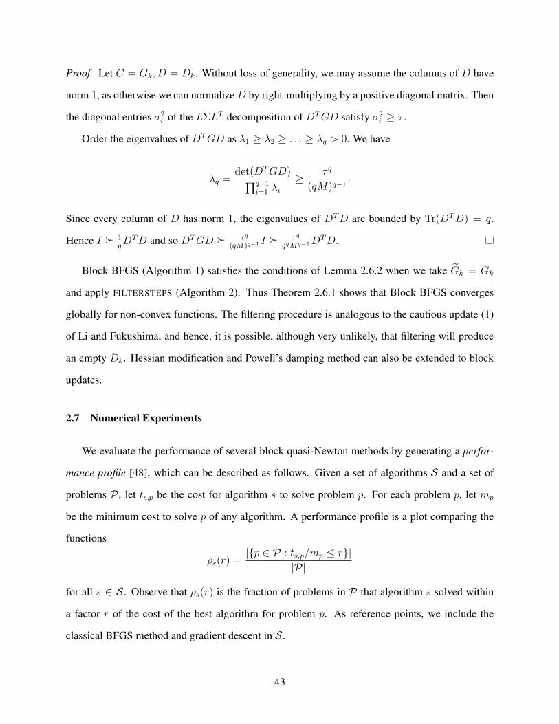
Proof. Let G = Gk, D = Dk. Without loss of generality, we may assume the columns of D have
norm 1, as otherwise we can normalizeD by right-multiplying by a positive diagonal matrix. Then
the diagonal entries σ2i of the LΣLT decomposition of DTGD satisfy σ2
i ≥ τ .
Order the eigenvalues of DTGD as λ1 ≥ λ2 ≥ . . . ≥ λq > 0. We have
λq =det(DTGD)∏q−1
i=1 λi≥ τ q
(qM)q−1.
Since every column of D has norm 1, the eigenvalues of DTD are bounded by Tr(DTD) = q.
Hence I 1qDTD and so DTGD τq
(qM)q−1 I τq
qqMq−1DTD.
Block BFGS (Algorithm 1) satisfies the conditions of Lemma 2.6.2 when we take Gk = Gk
and apply FILTERSTEPS (Algorithm 2). Thus Theorem 2.6.1 shows that Block BFGS converges
globally for non-convex functions. The filtering procedure is analogous to the cautious update (1)
of Li and Fukushima, and hence, it is possible, although very unlikely, that filtering will produce
an empty Dk. Hessian modification and Powell’s damping method can also be extended to block
updates.
2.7 Numerical Experiments
We evaluate the performance of several block quasi-Newton methods by generating a perfor-
mance profile [48], which can be described as follows. Given a set of algorithms S and a set of
problems P , let ts,p be the cost for algorithm s to solve problem p. For each problem p, let mp
be the minimum cost to solve p of any algorithm. A performance profile is a plot comparing the
functions
ρs(r) =|p ∈ P : ts,p/mp ≤ r|
|P|
for all s ∈ S . Observe that ρs(r) is the fraction of problems in P that algorithm s solved within
a factor r of the cost of the best algorithm for problem p. As reference points, we include the
classical BFGS method and gradient descent in S .
43

For our inexact line search, we used the function WolfeLineSearch from minFunc [49], a
mature and widely used Matlab library for unconstrained optimization. The line search parameters
were α = 0.1 and β = 0.75, and WolfeLineSearchwas configured to use interpolation with an
initial step size λ = 1 (options LS_type = 1,LS_init = 0,LS_interp = 1,LS_multi =
0).
From preliminary experiments, we found that large values of q tend to increase numerical
errors, eventually leading to search directions dk that are not descent directions. This effect is par-
ticularly pronounced when q ≥√n. The experiments in [31] also obtained the best performance
when bn1/4c ≤ q ≤√n. In creating performance profiles, we opted for q = bn1/3c.
2.7.1 Convex Experiments
We compared the methods listed below.
1. BFGS
2. Block BFGS Variant 1, or B-BFGS1
Block BFGS (Algorithm 1). We store the full inverse Hessian approximation Hk and com-
pute dk = −Hkgk by a matrix-vector product. We do not perform FILTERSTEPS, so the
update (2.3.4) uses all steps.
3. Block BFGS Variant 2, or B-BFGS2
Block BFGS (Algorithm 1), with Algorithm 2 and τ = 10−3. As in B-BFGS1, the full
Hessian approximation Hk is stored. Hk is updated by (2.3.4) using the steps returned by
Algorithm 2.
4. Block BFGS with q = 1, or B-BFGS-q1
This compares the effect of using a single sketching equation as in Block BFGS updates
versus using the standard secant equation of BFGS updates.
5. Rolling Block BFGS, or RB-BFGS
44
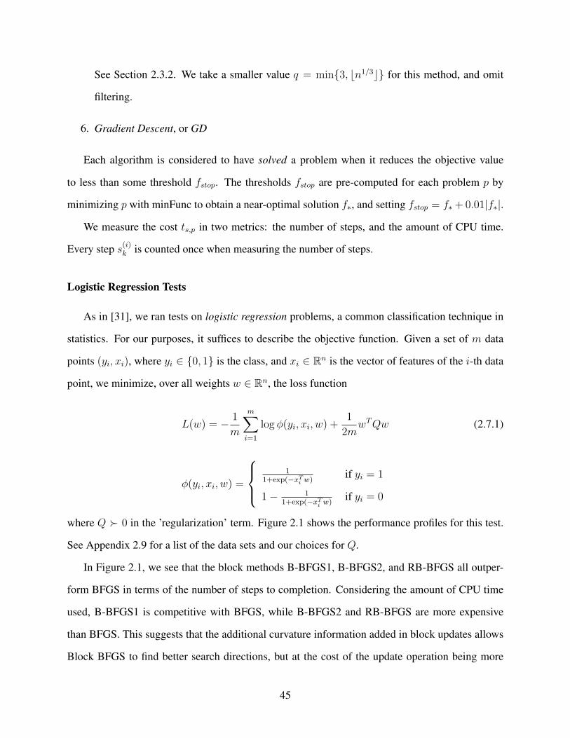
See Section 2.3.2. We take a smaller value q = min3, bn1/3c for this method, and omit
filtering.
6. Gradient Descent, or GD
Each algorithm is considered to have solved a problem when it reduces the objective value
to less than some threshold fstop. The thresholds fstop are pre-computed for each problem p by
minimizing p with minFunc to obtain a near-optimal solution f∗, and setting fstop = f∗+ 0.01|f∗|.
We measure the cost ts,p in two metrics: the number of steps, and the amount of CPU time.
Every step s(i)k is counted once when measuring the number of steps.
Logistic Regression Tests
As in [31], we ran tests on logistic regression problems, a common classification technique in
statistics. For our purposes, it suffices to describe the objective function. Given a set of m data
points (yi, xi), where yi ∈ 0, 1 is the class, and xi ∈ Rn is the vector of features of the i-th data
point, we minimize, over all weights w ∈ Rn, the loss function
L(w) = − 1
m
m∑i=1
log φ(yi, xi, w) +1
2mwTQw (2.7.1)
φ(yi, xi, w) =
1
1+exp(−xTi w)if yi = 1
1− 11+exp(−xTi w)
if yi = 0
where Q 0 in the ’regularization’ term. Figure 2.1 shows the performance profiles for this test.
See Appendix 2.9 for a list of the data sets and our choices for Q.
In Figure 2.1, we see that the block methods B-BFGS1, B-BFGS2, and RB-BFGS all outper-
form BFGS in terms of the number of steps to completion. Considering the amount of CPU time
used, B-BFGS1 is competitive with BFGS, while B-BFGS2 and RB-BFGS are more expensive
than BFGS. This suggests that the additional curvature information added in block updates allows
Block BFGS to find better search directions, but at the cost of the update operation being more
45
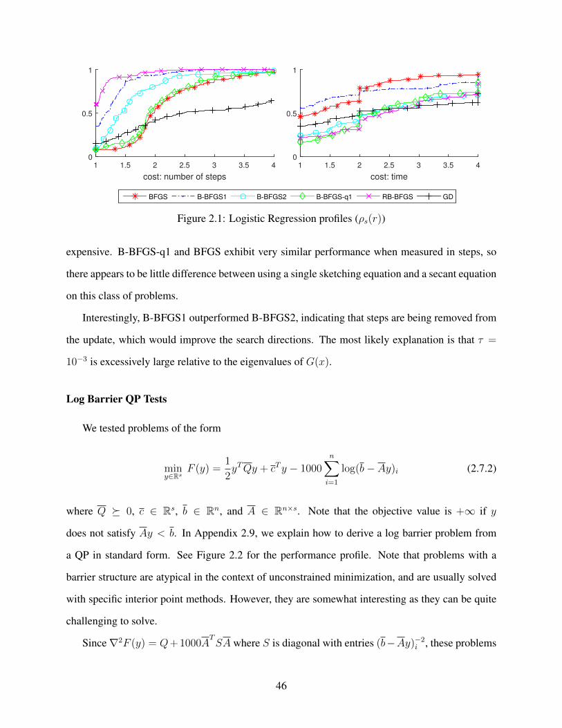
cost: number of steps
1 1.5 2 2.5 3 3.5 40
0.5
1
BFGS B-BFGS1 B-BFGS2 B-BFGS-q1 RB-BFGS GD
cost: time
1 1.5 2 2.5 3 3.5 40
0.5
1
Figure 2.1: Logistic Regression profiles (ρs(r))
expensive. B-BFGS-q1 and BFGS exhibit very similar performance when measured in steps, so
there appears to be little difference between using a single sketching equation and a secant equation
on this class of problems.
Interestingly, B-BFGS1 outperformed B-BFGS2, indicating that steps are being removed from
the update, which would improve the search directions. The most likely explanation is that τ =
10−3 is excessively large relative to the eigenvalues of G(x).
Log Barrier QP Tests
We tested problems of the form
miny∈Rs
F (y) =1
2yTQy + cTy − 1000
n∑i=1
log(b− Ay)i (2.7.2)
where Q 0, c ∈ Rs, b ∈ Rn, and A ∈ Rn×s. Note that the objective value is +∞ if y
does not satisfy Ay < b. In Appendix 2.9, we explain how to derive a log barrier problem from
a QP in standard form. See Figure 2.2 for the performance profile. Note that problems with a
barrier structure are atypical in the context of unconstrained minimization, and are usually solved
with specific interior point methods. However, they are somewhat interesting as they can be quite
challenging to solve.
Since∇2F (y) = Q+ 1000ATSA where S is diagonal with entries (b−Ay)−2
i , these problems
46
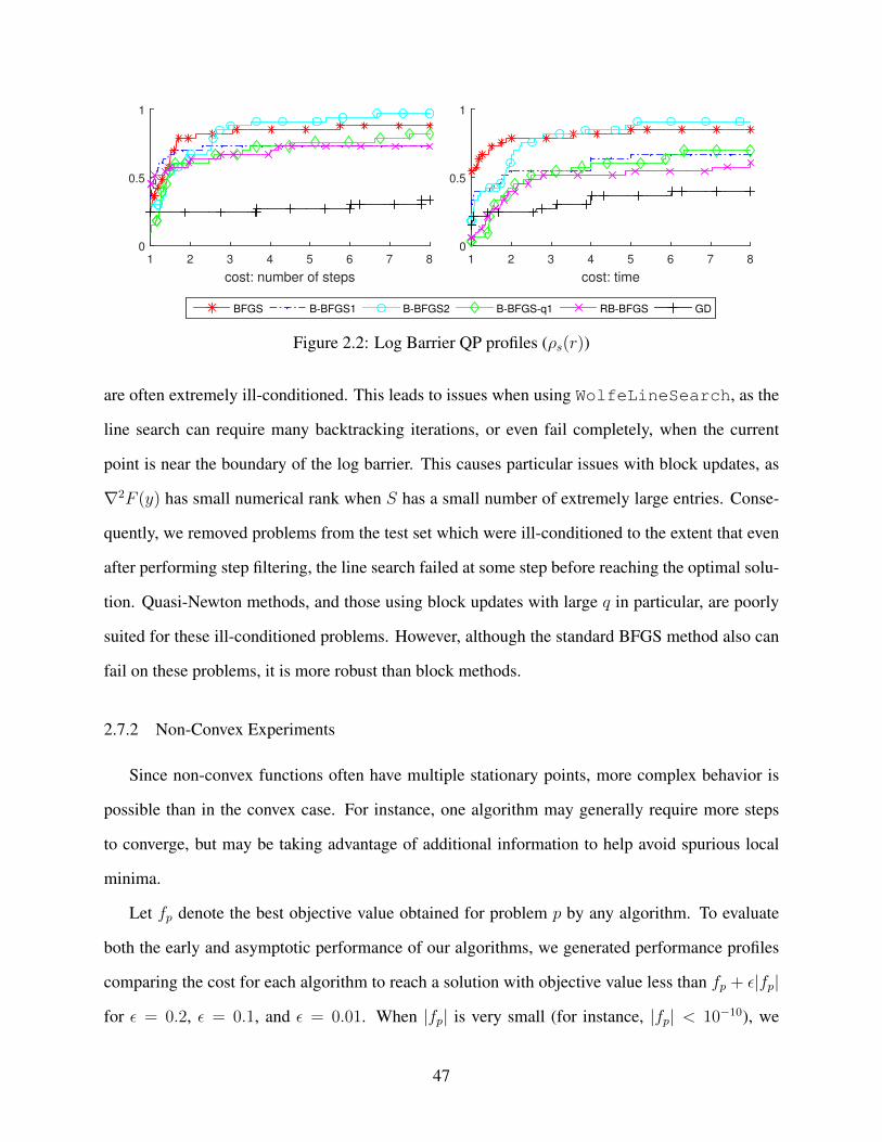
cost: number of steps
1 2 3 4 5 6 7 80
0.5
1
BFGS B-BFGS1 B-BFGS2 B-BFGS-q1 RB-BFGS GD
cost: time
1 2 3 4 5 6 7 80
0.5
1
Figure 2.2: Log Barrier QP profiles (ρs(r))
are often extremely ill-conditioned. This leads to issues when using WolfeLineSearch, as the
line search can require many backtracking iterations, or even fail completely, when the current
point is near the boundary of the log barrier. This causes particular issues with block updates, as
∇2F (y) has small numerical rank when S has a small number of extremely large entries. Conse-
quently, we removed problems from the test set which were ill-conditioned to the extent that even
after performing step filtering, the line search failed at some step before reaching the optimal solu-
tion. Quasi-Newton methods, and those using block updates with large q in particular, are poorly
suited for these ill-conditioned problems. However, although the standard BFGS method also can
fail on these problems, it is more robust than block methods.
2.7.2 Non-Convex Experiments
Since non-convex functions often have multiple stationary points, more complex behavior is
possible than in the convex case. For instance, one algorithm may generally require more steps
to converge, but may be taking advantage of additional information to help avoid spurious local
minima.
Let fp denote the best objective value obtained for problem p by any algorithm. To evaluate
both the early and asymptotic performance of our algorithms, we generated performance profiles
comparing the cost for each algorithm to reach a solution with objective value less than fp + ε|fp|
for ε = 0.2, ε = 0.1, and ε = 0.01. When |fp| is very small (for instance, |fp| < 10−10), we
47

essentially have fp = 0 and treat all solutions with objective value within 10−10 as being optimal.
We compared four different algorithms for non-convex minimization:
1. Damped BFGS, or D-BFGS
Damped BFGS with φ = 0.2 (see Section 2.6).
2. Block BFGS, or B-BFGS
Block BFGS (Algorithm 1) with q = bn1/3c and τ = 10−5.
3. Block BFGS with q = 1, or B-BFGS-q1
Block BFGS (Algorithm 1) with q = 1 and τ = 10−5.
4. Gradient Descent, or GD
Hyperbolic Tangent Loss Tests
This is also a classification technique; however, unlike the logistic regression problems in Sec-
tion 2.7.1, these problems are generally non-convex. Given a set of m data points (yi, xi) where
yi ∈ 0, 1 is the class, and xi ∈ Rn the features, we seek to minimize over w ∈ Rn the loss
function
L(w) =1
m
m∑i=1
(1− tanh(yix
Ti w)
)+
1
2m‖w‖2
Figure 2.3 presents performance profiles for ε = 0.2, 0.1, 0.01, with cost measured in both steps
and CPU time. See Appendix 2.9 for a list of the data sets.
B-BFGS and gradient descent perform well at first, making rapid progress to within 0.2|fp| of
fp in the fewest number of steps. B-BFGS continues to converge quickly, generally requiring the
fewest steps to reach 0.1|fp| and 0.01|fp| of fp, while gradient descent is overtaken by BFGS and
B-BFGS-q1.
Surprisingly, all four algorithms used nearly the same amount of CPU time, with each algorithm
completing a majority of problems after using only 1% more time than the fastest algorithm.
48

cost: number of steps
1 2 3 40
0.5
1
cost: number of steps
1 2 3 40
0.5
1
cost: number of steps
1 2 3 40
0.5
1
cost: time
1 1.005 1.010
0.5
1
cost: time
1 1.005 1.010
0.5
1
cost: time
1 1.005 1.010
0.5
1
D-BFGS B-BFGS B-BFGS-q1 GD
ǫ = 0.2 ǫ = 0.1 ǫ = 0.01
ǫ = 0.2 ǫ = 0.1 ǫ = 0.01
Figure 2.3: Hyperbolic Tangent Loss profiles (ρs(r))
Standard Benchmark Tests
This test used 19 functions from the test collection of Andrei [50], many of which originate
from the CUTEst test set. The functions are listed below, with the number of variables n in paren-
theses:
arwhead (300), bdqrtic (200), cube (400), diag1 (250), dixonprice (200), edensch
(300), eg2 (400), explin2 (200), fletchcr (400), genhumps (250), indef (250), mccormick
(400), raydan1 (400), rosenbrock (300), sine (400), sinquad (400), tointgss (200),
trid (200), whiteholst (300).
The gradients and Hessians were computed using the automatic differentiation program ADi-
Gator [51].
For each of these functions, we generated 6 random starting points and tested the 4 algorithms
using each starting point, for a total of 114 problems. Figure 2.4 presents performance profiles for
ε = 0.2, 0.1, 0.01, with cost measured in steps. We see from Figure 2.4 that D-BFGS consistently
outperforms B-BFGS-q1, which suggests that Powell’s damping method is superior to cautious
updates.
49
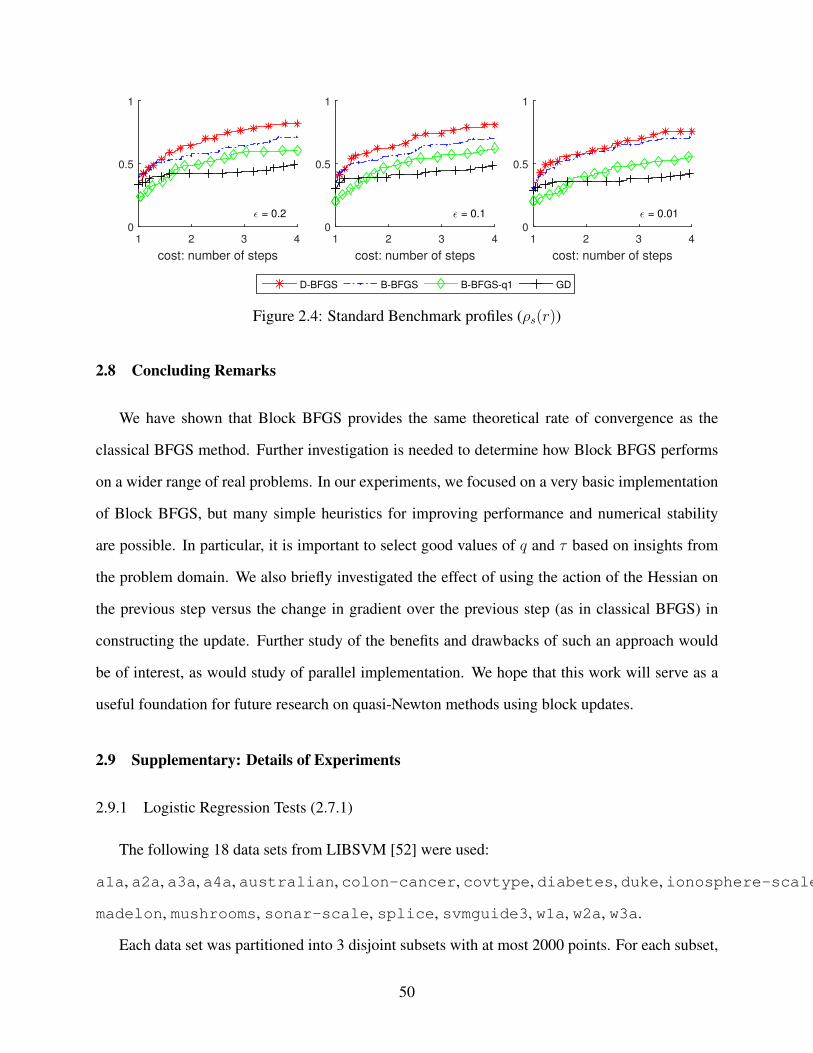
cost: number of steps
1 2 3 40
0.5
1
cost: number of steps
1 2 3 40
0.5
1
cost: number of steps
1 2 3 40
0.5
1
D-BFGS B-BFGS B-BFGS-q1 GD
ǫ = 0.2 ǫ = 0.1 ǫ = 0.01
Figure 2.4: Standard Benchmark profiles (ρs(r))
2.8 Concluding Remarks
We have shown that Block BFGS provides the same theoretical rate of convergence as the
classical BFGS method. Further investigation is needed to determine how Block BFGS performs
on a wider range of real problems. In our experiments, we focused on a very basic implementation
of Block BFGS, but many simple heuristics for improving performance and numerical stability
are possible. In particular, it is important to select good values of q and τ based on insights from
the problem domain. We also briefly investigated the effect of using the action of the Hessian on
the previous step versus the change in gradient over the previous step (as in classical BFGS) in
constructing the update. Further study of the benefits and drawbacks of such an approach would
be of interest, as would study of parallel implementation. We hope that this work will serve as a
useful foundation for future research on quasi-Newton methods using block updates.
2.9 Supplementary: Details of Experiments
2.9.1 Logistic Regression Tests (2.7.1)
The following 18 data sets from LIBSVM [52] were used:
a1a, a2a, a3a, a4a, australian, colon-cancer, covtype, diabetes, duke, ionosphere-scale,
madelon, mushrooms, sonar-scale, splice, svmguide3, w1a, w2a, w3a.
Each data set was partitioned into 3 disjoint subsets with at most 2000 points. For each subset,
50

we have a problem of the form (2.7.1) with the standard L2 regularizer Q = I , producing 54
standard problems. An additional 96 problems with Q = I + Q′ were produced by adding a
randomly generated convex quadraticQ′ to one of the standard problems. Two such problems were
produced for each standard problem, except those from duke and colon-cancer (omitted for
problem size).
2.9.2 Log Barrier QP Tests (2.7.1)
Given a convex quadratic program minx∈Rn1
2xTQx + cTx | Ax = b, x ≥ 0, we derive a log
barrier QP problem as follows. Taking a basis N for the null space of A (of dimension s), and a
solution Ax0 = b, x0 ≥ 0, the given QP is equivalent to miny∈Rs1
2yTQy + cTy | Ay ≤ b, where
Q = NTQN, c = NT (c + Qx0), b = x0 and A = −N . Replacing the constraint by a log barrier
−µ∑n
i=1 log(b− Ay)i (with µ = 1000), we obtain problem (2.7.2).
This test included 43 problems in total. There were 35 log barrier problems derived from the
QP test collection of Maros and Mészáros [53]:
cvxqp1_m, cvxqp1_s, cvxqp2_m, cvxqp2_s, cvxqp3_m, cvxqp3_s, dual1, dual2,
dual3, dual4, primal1, primal3, primal4, primalc1, primalc2, primalc5, primalc8,
q25fv47, qbeaconf, qgrow15, qgrow22, qgrow7, qisrael, qscagr7, qscfxm1, qscfxm2,
qscfxm3, qscorpio, qscrs8, qsctap1, qsctap3, qshare1b, qship08l, stadat1,
stadat2.
An additional 8 problems were derived from the following LP problems in the COAP collection
[54]: adlittle, agg, agg2, agg3, bnl1, brandy, fffff800, ganges.
2.9.3 Hyperbolic Tangent Loss Tests (2.7.2)
This test used the same data sets as the logistic regression test, with duke omitted because of
large problem size (n = 7130). As in the logistic regression test, each data set was partitioned into
3 subsets with at most 2000 points, producing 51 loss functions. For each loss function, we tried 4
random starting points, for a total of 204 problems.
51

Chapter 3: Superlinear Convergence Without Line Searches for
Self-Concordant Functions
3.1 Introduction
We are concerned in this paper with iterative optimization algorithms, which at each step, first
select a direction dk and then determine a step size tk. Such algorithms, which are usually referred
to as line search algorithms, need to choose an appropriate step size tk to perform well, both in
theory and in practice.
Theoretical proofs of global convergence generally assume one of the following approaches
for selecting the step sizes:
1. The step sizes are obtained from line searches.
2. The step size is a constant, often chosen ‘sufficiently small’.
Inexact line searches, and in particular those that choose steps that satisfy the Armijo-Wolfe con-
ditions, or just the latter combined with backtracking, are usually performed and work well in
practice. However, they can be costly to perform, and are often prohibitively costly for many
common objective functions such as those that arise in machine learning, computer vision, and
natural language processing. Moreover, in stochastic optimization algorithms, line searches based
on stochastic function values and gradients, which are only estimates of the true quantities (see
Section 3.8), can be meaningless. In contrast, constant step sizes tk = t for all k require no addi-
tional computation beyond selecting t, but determining an appropriate constant t may be difficult.
The value of t required in the theoretical analysis is often too small for practical purposes, and
moreover, is impossible to compute without knowledge of unknown parameters (e.g. the Lips-
chitz constant of ∇f ). A single constant step size may also be highly suboptimal, as the iterates
52

transition between regions with different curvature.
The basic idea for a step size determined by the local curvature of the objective function f
was developed by Nesterov, who introduced the damped Newton method [33]. This idea is closely
related to a well-behaved class of functions known as self-concordant functions [55], which we
define in Section 3.3. When applied to a self-concordant function f , the damped Newton method
is globally convergent and locally converges quadratically. These results were extended in recent
work.
1. Tran-Dinh et al. [56] propose a proximal framework for composite self-concordant min-
imization, which includes proximal damped Newton, proximal quasi-Newton, and proxi-
mal gradient descent. They establish that proximal damped Newton is globally convergent
and locally quadratically convergent, and that proximal damped gradient descent is globally
convergent and locally linearly convergent. However, they do not propose a proximal quasi-
Newton algorithm or prove global convergence for a generic version of such an algorithm.
2. Zhang and Xiao [57] propose a distributed method for self-concordant empirical loss func-
tions, based on the damped Newton method, and establish its convergence.
3. Lu [58] proposes a randomized block proximal damped Newton method for composite self-
concordant minimization, and establishes its convergence.
While the damped Newton method has been extensively studied, no comparable theory ex-
ists for quasi-Newton methods in the self-concordant setting. It is well known that for convex
functions, proving global convergence for the BFGS method [59, 25, 23, 26] with inexact line
searches is far more challenging than proving global convergence for scaled gradient methods,
and that a similar statement holds for the Q-superlinear convergence of the BFGS method applied
to strongly convex functions compared with, for example, proving Q-quadratic convergence of
Newton’s method. With regard to Q-superlinear convergence, it is well known [41] that if the the
largest eigenvalue of the Hessian of the objective is bounded above, and if the sum of the distances
of the iterates generated by the BFGS method from the global minimizer is finite, then the BFGS
53
method converges Q-superlinearly. We note that Tran-Dinh et al. [56] give a proof of this local
result for their “pure"-proximal-BFGS method (i.e., one that uses a step size of 1 on every iteration
and starts from a point “close" to the global minimizer), but they do not prove that this method
generates iterates satisfying the required conditions. This leaves open the question of how to de-
sign a globally convergent “dampled” version of the BFGS method for self-concordant functions.
In particular, we wish to avoid assuming either the Dennis-Moré condition [43] or the summability
of the distances to the global minmizer, since these conditions are extremely strong, verging on
being tautological, as assumptions.
In this paper we extend the theory of self-concordant minimization developed by Nesterov and
Nemirovski [55] and further developed by Tran-Dinh et al. [56]. Our focus here is mainly on
filling the gap in this theory for quasi-Newton methods. To simplify the presentation, we consider
only quasi-Newton methods that use the BFGS update, although our results apply to all methods in
the Broyden class of quasi-Newton methods other than the DFP method [28, 29]. We introduce a
framework for non-composite optimization; i.e., we do not consider proximal methods as in [56].
The key feature of this framework is a step size that is optimal with respect to an upper bound on
the decrease in the objective value, which we call the curvature-adaptive step size. We use the term
curvature-adaptive, or simply adaptive, to refer to this step size choice or to methods that employ
it, so as not to confuse such methods with damped BFGS updating methods (e.g., see [60, §18.3]),
which are unrelated.
We first prove that scaled gradient methods that use the curvature-adaptive step size are glob-
ally R-linearly convergent on strongly convex self-concordant functions. We note that in [56],
this step size is also identified, but that the R-linear convergence is only proved locally. We then
prove our main result, on quasi-Newton methods: that the BFGS method, using this step size, is
globally convergent for functions that are self-concordant, bounded below, and have a bounded
Hessian, and furthermore, is Q-superlinearly convergent when the function is strongly convex and
self-concordant. For completeness, we then present several numerical experiments which shed in-
sight on the behavior of adaptive methods. These show that for deterministic optimization, using
54

curvature-based step sizes in quasi-Newton methods is dominated by using inexact line searches,
whereas in stochastic settings, using curvature-based step sizes is very helpful compared to con-
stant step sizes.
Our paper is organized as follows. In Section 3.2, we introduce the notation and assump-
tions that we use throughout the paper. In Section 3.3, we define the class of self-concordant
functions and describe their essential properties. In Section 3.4, we introduce our framework for
self-concordant minimization and provide a derivation of what we call the curvature-adaptive step
size, which extends the curvature-based step size obtained in [56] for proximal gradient methods.
In Section 3.5, we apply our approach to scaled gradient methods, and give a simple proof that
these methods are globally R-linearly convergent on strongly convex self-concordant functions.
In Section 3.6, we present our main results. Specifically, we prove there that the BFGS method
with curvature-adaptive step sizes is globally and Q-superlinearly convergent. In Section 3.8, we
discuss stochastic extensions of adaptive methods. In Section 3.9.1, we present numerical ex-
periments testing our new methods on logistic regression problems in the deterministic setting.
In Section 3.9.2, we provide a numerical example of solving an online stochastic problem using
stochastic adaptive methods.
3.2 Preliminaries
We use f : Rn → R to denote the objective function, and g(·), G(·) denote the gradient ∇f(·)
and Hessian ∇2f(·), respectively. In the context of a sequence of points xk∞k=0, we write gk for
g(xk) and Gk for G(xk). Unless stated otherwise, the function f is assumed to have continuous
third derivatives (as f is generally assumed to be self-concordant), which we write as f ∈ C3.
The norm ‖ · ‖ denotes the 2-norm, and when applied to a matrix, the operator 2-norm.
3.3 Self-Concordant Functions
The notion of self-concordant functions was first introduced by Nesterov and Nemirovski [55]
for their analysis of Newton’s method in the context of interior-point methods. Nesterov [33]
55
provides a clear exposition and motivates self-concordancy by observing that, while Newton’s
method is invariant under affine transformations, the convergence analysis makes use of norms
which are not invariant. To remedy this, Nesterov and Nemirovski replace the Euclidean norm by
an invariant local norm, and replace the assumption of Lipschitz continuity of the Hessian G(x) by
the self-concordancy of f .
Definition. Let f be a convex function. The local norm of h ∈ Rn at a point x where G(x) 0 is
given by
‖h‖x =√hTG(x)h.
Definition. A closed convex function f : Rn → R is self-concordant if f ∈ C3 and there exists a
constant κ such that for every x ∈ Rn and every h ∈ Rn, we have
|∇3f(x)[h, h, h]| ≤ κ(∇2f(x)[h, h])3/2.
If κ = 2, f is standard self-concordant. Any self-concordant function can be scaled to be standard
self-concordant; the scaled function 14κ2f is standard self-concordant. Hence, we assume all self-
concordant functions have κ = 2, unless stated otherwise.
There is also an equivalent definition which is frequently useful.
Theorem 3.3.1 (Lemma 4.1.2, [33]). A closed convex function f is self-concordant if and only if
for every x ∈ Rn and all u1, u2, u3 ∈ Rn, we have
|∇3f(x)[u1, u2, u3]| ≤ 23∏i=1
‖ui‖x.
The next inequalities are fundamental for self-concordant functions. These results are well
known (see [33, §4.1.4]), but for completeness, we provide a proof.
Lemma 3.3.2. Let f be standard self-concordant and strictly convex, and let x ∈ Rn and 0 6= d ∈
56
Rn. Let δ = ‖d‖x. Then for all t ≥ 0,
f(x+ td) ≥ f(x) + tg(x)Td+ δt− log(1 + δt) (3.3.1)
and
g(x+ td)Td ≥ g(x)Td+δ2t
1 + δt. (3.3.2)
For all 0 ≤ t < 1δ,
f(x+ td) ≤ f(x) + tg(x)Td− δt− log(1− δt) (3.3.3)
and
g(x+ td)Td ≤ g(x)Td+δ2t
1− δt. (3.3.4)
Proof. Define φ : R → R by φ(t) = dT∇2f(x + td)d. Since f has continuous third deriva-
tives, φ(t) is continuously differentiable and from the definition of self-concordancy, its derivative
satisfies
|φ′(t)| = |∇3f(x+ td)[d, d, d]| ≤ 2(∇2f(x+ td)[d, d])3/2 = 2φ(t)3/2. (3.3.5)
Moreover, since f is strictly convex and d 6= 0, φ(t) > 0 for all t. Therefore, from (3.3.5),
| ddtφ(t)−1/2| = 1
2|φ(t)−3/2φ′(t)| ≤ 1.
Defining ψ(s) = ddtφ(t)−1/2
∣∣t=s
, the above inequality is equivalent to |ψ(s)| ≤ 1. By Taylor’s
Theorem, there exists a point u ∈ (0, t) such that φ(t)−1/2 − φ(0)−1/2 = tψ(u). Since |ψ(u)| ≤ 1,
we deduce that
φ(0)−1/2 − t ≤ φ(t)−1/2 ≤ φ(0)−1/2 + t.
Note that δ = φ(0)1/2. Rearranging the upper bound, we find that for all t ≥ 0,
φ(t) ≥ δ2
(1 + δt)2. (3.3.6)
57

Similarly, we find that for 0 ≤ t < 1δ,
φ(t) ≤ δ2
(1− δt)2. (3.3.7)
Integrating (3.3.6) yields the inequalities (3.3.1), (3.3.2), and integrating (3.3.7) produces (3.3.3),
(3.3.4).
3.4 Curvature-Adaptive Step Sizes
We define a general framework for an iterative method with step sizes determined by the local
curvature. At each step, we compute a descent direction dk = −Hkgk, where Hk is a positive
definite matrix, and a step size
tk =ρk
(ρk + δk)δk,
where
δk = ‖dk‖xk
and
ρk = gTkHkgk.
We then advance to the point xk+1 = xk + tkdk.
We will refer to the above step size tk as the curvature-adaptive step size, or simply the adaptive
step size. A method within our framework will be referred to as an adaptive method. A generic
method in this framework is specified in Algorithm 3.
Note that this framework encompasses several classical methods. When Hk = I for all k, the
resulting method is gradient descent. When Hk = G−1k , we recover the damped Newton method
proposed by Nesterov. WhenHk is an approximation ofG−1k obtained by applying a quasi-Newton
updating formula, the resulting method is a quasi-Newton method. In particular, we will focus on
the case where Hk evolves according to the BFGS update formula. We also note that in all variants
other than the damped Newton method, we do not access the full Hessian matrixGk at any step, but
58
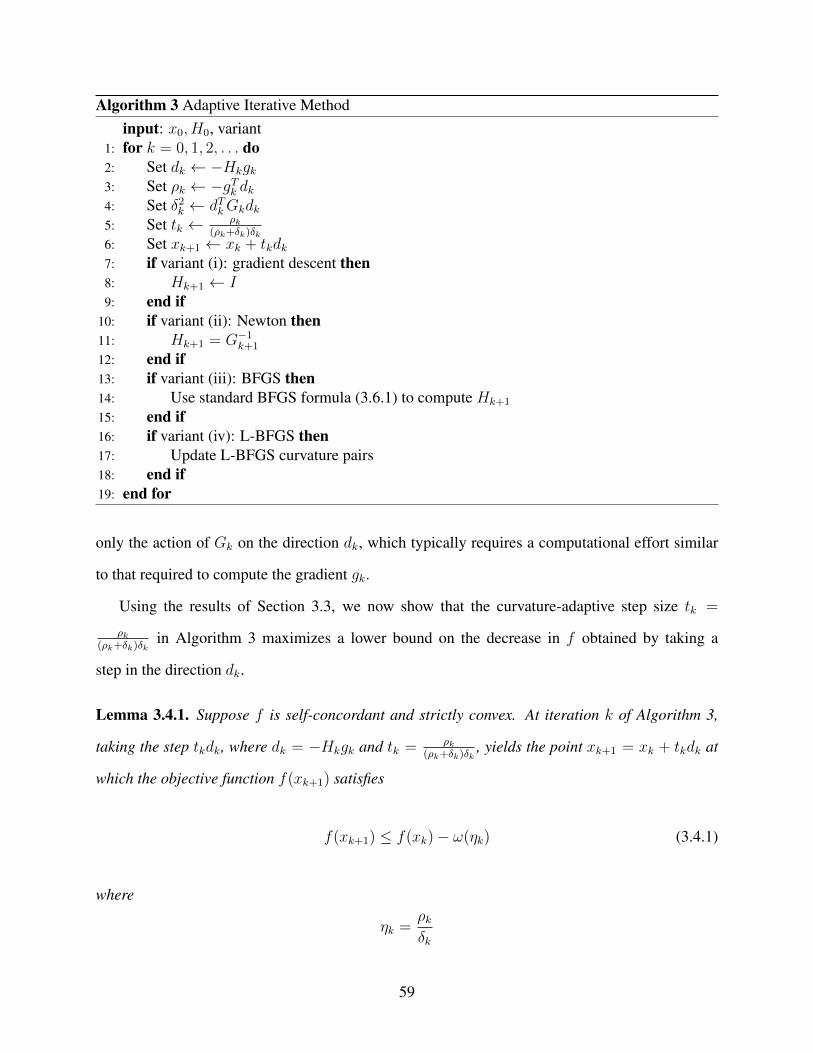
Algorithm 3 Adaptive Iterative Methodinput: x0, H0, variant
1: for k = 0, 1, 2, . . . do2: Set dk ← −Hkgk3: Set ρk ← −gTk dk4: Set δ2
k ← dTkGkdk5: Set tk ← ρk
(ρk+δk)δk6: Set xk+1 ← xk + tkdk7: if variant (i): gradient descent then8: Hk+1 ← I9: end if
10: if variant (ii): Newton then11: Hk+1 = G−1
k+1
12: end if13: if variant (iii): BFGS then14: Use standard BFGS formula (3.6.1) to compute Hk+1
15: end if16: if variant (iv): L-BFGS then17: Update L-BFGS curvature pairs18: end if19: end for
only the action of Gk on the direction dk, which typically requires a computational effort similar
to that required to compute the gradient gk.
Using the results of Section 3.3, we now show that the curvature-adaptive step size tk =
ρk(ρk+δk)δk
in Algorithm 3 maximizes a lower bound on the decrease in f obtained by taking a
step in the direction dk.
Lemma 3.4.1. Suppose f is self-concordant and strictly convex. At iteration k of Algorithm 3,
taking the step tkdk, where dk = −Hkgk and tk = ρk(ρk+δk)δk
, yields the point xk+1 = xk + tkdk at
which the objective function f(xk+1) satisfies
f(xk+1) ≤ f(xk)− ω(ηk) (3.4.1)
where
ηk =ρkδk
59

and ω : R→ R is the function ω(z) = z − log(1 + z).
Moreover, the step size tk minimizes the upper bound (3.3.3) on f(xk+1) provided by Lemma 3.3.2.
Proof. We fix the index k and omit the subscripts for brevity. First, observe that
0 ≤ t =ρ
(ρ+ δ)δ<
1
δ.
Therefore, we can apply inequality (3.3.3) to f(x + td). Noting that ρ = −gTd, (3.3.3) can be
written as f(x + td) ≤ f(x)−∆(t) where ∆(·) is defined to be the function ∆(τ) = (ρ + δ)τ +
log(1− δτ). For the curvature-adaptive step size t, it is easily verified that
∆(t) = ∆
(ρ
(ρ+ δ)δ
)=ρ
δ+ log
(δ
ρ+ δ
)=ρ
δ− log
(1 +
ρ
δ
)= ω(η).
Furthermore, for 0 ≤ τ < 1δ, ddτ
∆(τ) = ρ + δ − δ1−δτ and d2
dτ2∆(τ) = − δ2
(1−δτ)2. We find that
ddτ
∆(t) = 0 and d2
dτ2∆(t) ≤ 0, which implies that ∆ is maximized at τ = t = ρ
(ρ+δ)δ.
Since ω(η) = η − log(1 + η) is positive for all η > 0, it follows that if lim supk ηk > 0, then
f(xk)→ −∞. This simple fact will be crucial in our convergence analysis.
Lemma 3.4.2. If, in addition to the assumptions in Lemma 3.4.1, f is bounded below, then ηk =
ρkδk→ 0 for any of the adaptive variants in Algorithm 3.
Proof. By Lemma 3.4.1, f(xk) satisfies f(xk) ≤ f(x0)−∑k−1
j=0 ω(ηj). Suppose that lim supk ηk >
0. Since the function ω(η) is positive and monotonically increasing for η > 0, we have lim supk ω(ηk) =
ω(lim supk ηk) > 0. Hence f(xk)→ −∞, a contradiction.
In terms of gk, Hk, and Gk, the adaptive step size tk can be expressed as
tk =gTkHkgk
gTkHkGkHkgk + gTkHkgk√gTkHkGkHkgk
.
This formula relates tk to the local curvature. When the curvature of f in the direction dk = −Hkgk
is relatively flat, the local norm ‖dk‖xk =√gTkHkGkHkgk is small, and the adaptive step size tk
60
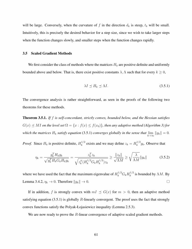
will be large. Conversely, when the curvature of f in the direction dk is steep, tk will be small.
Intuitively, this is precisely the desired behavior for a step size, since we wish to take larger steps
when the function changes slowly, and smaller steps when the function changes rapidly.
3.5 Scaled Gradient Methods
We first consider the class of methods where the matricesHk are positive definite and uniformly
bounded above and below. That is, there exist positive constants λ,Λ such that for every k ≥ 0,
λI Hk ΛI. (3.5.1)
The convergence analysis is rather straightforward, as seen in the proofs of the following two
theorems for these methods.
Theorem 3.5.1. If f is self-concordant, strictly convex, bounded below, and the Hessian satisfies
G(x) MI on the level set Ω = x : f(x) ≤ f(x0), then any adaptive method (Algorithm 3) for
which the matrices Hk satisfy equation (3.5.1) converges globally in the sense that limk→∞‖gk‖ = 0.
Proof. Since Hk is positive definite, H1/2k exists and we may define zk = H
1/2k gk. Observe that
ηk =gTkHkgk√
gTkHkGkHkgk=
zTk zk√zTk (H
1/2k GkH
1/2k )zk
≥ ‖zk‖√ΛM
≥√
λ
ΛM‖gk‖ (3.5.2)
where we have used the fact that the maximum eigenvalue of H1/2k GkH
1/2k is bounded by ΛM . By
Lemma 3.4.2, ηk → 0. Therefore ‖gk‖ → 0.
If in addition, f is strongly convex with mI G(x) for m > 0, then an adaptive method
satisfying equation (3.5.1) is globally R-linearly convergent. The proof uses the fact that strongly
convex functions satisfy the Polyak-Łojasiewicz inequality (Lemma 2.5.3).
We are now ready to prove the R-linear convergence of adaptive scaled gradient methods.
61

Theorem 3.5.2. If f is self-concordant and strongly convex (so there exist constants 0 < m ≤ M
such that mI G(x) MI for all x ∈ Ω), then an adaptive method (Algorithm 3) for which
the matrices Hk satisfy equation (3.5.1) is globally R-linearly convergent. That is, there exists a
positive constant γ < 1 such that f(xk+1)− f(x∗) ≤ γ(f(xk)− f(x∗)) for all k.
Proof. Since ηk → 0 by Lemma 3.4.2, the sequence ηk∞k=0 is bounded. Let Γ = supk ηk < ∞,
and let c = 12(1+Γ)
. Observe that ω(z) = z − log(1 + z) ≥ cz2 for 0 ≤ z ≤ Γ, as ω(0) = 0 and
ddz
(ω(z)− cz2) = z(1−2c−2cz)1+z
, which is non-negative for 0 ≤ z ≤ Γ. Hence, since ηk ≤ Γ for all k,
we have
f(xk+1)− f(x∗) ≤ f(xk)− f(x∗)− ω(ηk) ≤ f(xk)− f(x∗)− cη2k
≤ f(xk)− f(x∗)−cλ
ΛM‖g(xk)‖2
≤(
1− λm
Λ(1 + Γ)M
)(f(xk)− f(x∗))
where the first line follows from inequality (3.3.3), the second from inequality (3.5.2), and the third
from Lemma 2.5.3. Taking γ = 1− λmΛ(1+Γ)M
, we obtain the desired R-linear convergence.
3.5.1 Adaptive Gradient Descent
When Hk = I for all k in Algorithm 3, the method corresponds to gradient descent with adap-
tive step sizes that incorporate second-order information. This strategy for selecting analytically
computable step sizes may have several advantages in practice. Using second-order information al-
lows a better local model of the objective function. The classical analysis of gradient descent with
a fixed step size also generally requires a sufficiently small step size in order to guarantee conver-
gence. This step size is a function of the Lipschitz constant for the gradient g(x), which is either
unknown or impractical to compute. The step size needed to ensure convergence in theory is also
often impractically tiny, leading to slow convergence in practice. For the class of self-concordant
functions, an adaptive step size can be easily computed without knowledge of any constants, and
still provides a theoretical guarantee of convergence, which is a significant advantage.
62
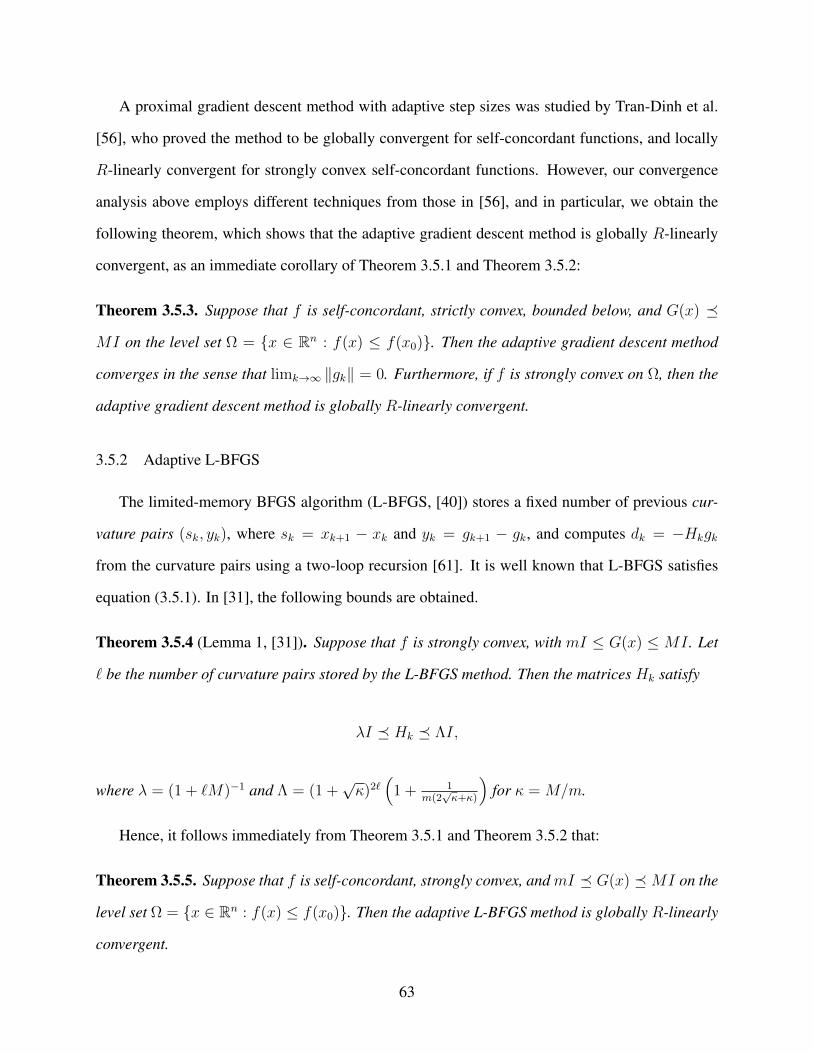
A proximal gradient descent method with adaptive step sizes was studied by Tran-Dinh et al.
[56], who proved the method to be globally convergent for self-concordant functions, and locally
R-linearly convergent for strongly convex self-concordant functions. However, our convergence
analysis above employs different techniques from those in [56], and in particular, we obtain the
following theorem, which shows that the adaptive gradient descent method is globally R-linearly
convergent, as an immediate corollary of Theorem 3.5.1 and Theorem 3.5.2:
Theorem 3.5.3. Suppose that f is self-concordant, strictly convex, bounded below, and G(x)
MI on the level set Ω = x ∈ Rn : f(x) ≤ f(x0). Then the adaptive gradient descent method
converges in the sense that limk→∞ ‖gk‖ = 0. Furthermore, if f is strongly convex on Ω, then the
adaptive gradient descent method is globally R-linearly convergent.
3.5.2 Adaptive L-BFGS
The limited-memory BFGS algorithm (L-BFGS, [40]) stores a fixed number of previous cur-
vature pairs (sk, yk), where sk = xk+1 − xk and yk = gk+1 − gk, and computes dk = −Hkgk
from the curvature pairs using a two-loop recursion [61]. It is well known that L-BFGS satisfies
equation (3.5.1). In [31], the following bounds are obtained.
Theorem 3.5.4 (Lemma 1, [31]). Suppose that f is strongly convex, with mI ≤ G(x) ≤ MI . Let
` be the number of curvature pairs stored by the L-BFGS method. Then the matrices Hk satisfy
λI Hk ΛI,
where λ = (1 + `M)−1 and Λ = (1 +√κ)2`
(1 + 1
m(2√κ+κ)
)for κ = M/m.
Hence, it follows immediately from Theorem 3.5.1 and Theorem 3.5.2 that:
Theorem 3.5.5. Suppose that f is self-concordant, strongly convex, andmI G(x) MI on the
level set Ω = x ∈ Rn : f(x) ≤ f(x0). Then the adaptive L-BFGS method is globally R-linearly
convergent.
63
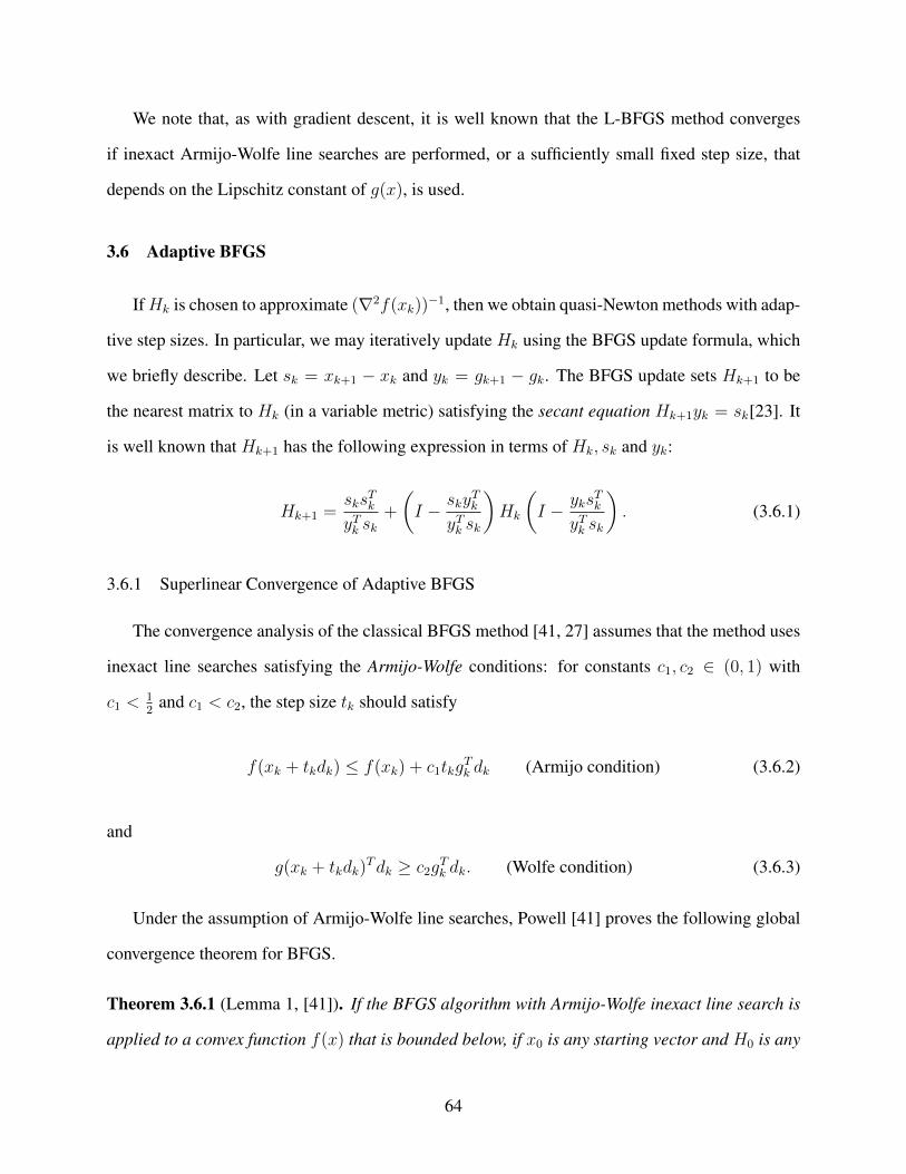
We note that, as with gradient descent, it is well known that the L-BFGS method converges
if inexact Armijo-Wolfe line searches are performed, or a sufficiently small fixed step size, that
depends on the Lipschitz constant of g(x), is used.
3.6 Adaptive BFGS
IfHk is chosen to approximate (∇2f(xk))−1, then we obtain quasi-Newton methods with adap-
tive step sizes. In particular, we may iteratively update Hk using the BFGS update formula, which
we briefly describe. Let sk = xk+1 − xk and yk = gk+1 − gk. The BFGS update sets Hk+1 to be
the nearest matrix to Hk (in a variable metric) satisfying the secant equation Hk+1yk = sk[23]. It
is well known that Hk+1 has the following expression in terms of Hk, sk and yk:
Hk+1 =sks
Tk
yTk sk+
(I − sky
Tk
yTk sk
)Hk
(I − yks
Tk
yTk sk
). (3.6.1)
3.6.1 Superlinear Convergence of Adaptive BFGS
The convergence analysis of the classical BFGS method [41, 27] assumes that the method uses
inexact line searches satisfying the Armijo-Wolfe conditions: for constants c1, c2 ∈ (0, 1) with
c1 <12
and c1 < c2, the step size tk should satisfy
f(xk + tkdk) ≤ f(xk) + c1tkgTk dk (Armijo condition) (3.6.2)
and
g(xk + tkdk)Tdk ≥ c2g
Tk dk. (Wolfe condition) (3.6.3)
Under the assumption of Armijo-Wolfe line searches, Powell [41] proves the following global
convergence theorem for BFGS.
Theorem 3.6.1 (Lemma 1, [41]). If the BFGS algorithm with Armijo-Wolfe inexact line search is
applied to a convex function f(x) that is bounded below, if x0 is any starting vector and H0 is any
64
positive definite matrix, and if the Hessian G(x) satisfies G(x) MI for all x in the level set
Ω = x : f(x) ≤ f(x0), then the limit
lim infk→∞
‖gk‖ = 0 (3.6.4)
is obtained.
In our setting, f is a self-concordant and strictly convex function that is bounded below and
satisfies G(x) MI . In order to prove that adaptive BFGS is convergent in the sense of the
limit (3.6.4), it suffices to show that the adaptive step sizes tk satisfy the Armijo condition for
any c1 <12, and eventually satisfy the Wolfe condition for any c2 < 1 (i.e. there exists some k0
such that the Wolfe condition is satisfied for all k ≥ k0). Specifically, we prove the following two
theorems that apply to every adaptive method described by Algorithm 3.
Theorem 3.6.2. Let f be self-concordant and strictly convex. The curvature-adaptive step size
tk = ρk(ρk+δk)δk
satisfies the Armijo condition for any c1 ≤ 12.
Proof. Let c1 ≤ 12. We aim to prove that f(xk+1) ≤ f(xk) + c1tkg
Tk dk. By Lemma 3.4.1,
f(xk+1) ≤ f(xk)− ω(ηk). Therefore, it suffices to prove that
ω(ηk) ≥ −1
2tkg
Tk dk.
For brevity, we omit the index k. Notice that
−tgTd = tgTHg = tρ =ρ2
(ρ+ δ)δ=
ρ2/δ2
ρ/δ + 1=
η2
1 + η.
Therefore, we must prove that for η ≥ 0,
ω(η) = η − log(1 + η) ≥ 1
2
η2
1 + η.
65

Define ζ(z) = z − log(1 + z)− 12z2
1+z. Observe that ζ(0) = 0 and
d
dzζ(z) = 1− 1
1 + z− 1
2
z2 + 2z
(1 + z)2=
1
2
z2
(1 + z)2.
Since ddzζ(z) ≥ 0 for all z ≥ 0, we conclude that ω(η) ≥ 1
2η2
1+ηfor all η ≥ 0. This completes the
proof.
Theorem 3.6.3. Let f be self-concordant, strictly convex, and bounded below. Suppose that
xk∞k=0 is a sequence of iterates generated by Algorithm 3. For any 0 < c2 < 1, there exists
an index k0 such that for all k ≥ k0, the curvature-adaptive step size tk satisfies the Wolfe condi-
tion.
Proof. We aim to prove that gTk+1dk ≥ c2gTk dk. This is equivalent to g(xk+tkdk)
Tdk−g(xk)Tdk ≥
−(1− c2)g(xk)Tdk = (1− c2)ρk. By inequality (3.3.2) with δ = δk and t = tk, we have
g(xk + tkdk)Tdk − g(xk)
Tdk ≥δ2ktk
1 + δktk=
δkρk2ρk + δk
=1
1 + 2ηkρk. (3.6.5)
Since f is bounded below, Lemma 3.4.2 implies that η → 0, and hence there exists some k0 such
that 11+2ηk
≥ 1− c2 for all k ≥ k0.
Note that the assumption of strict convexity also implies that yTk sk > 0, so the BFGS update is
well-defined.
We can now immediately apply Theorem 3.6.1 to deduce that adaptive BFGS is convergent.
Since there always exists an index k0 such that the Armijo-Wolfe conditions are satisfied for all
k ≥ k0, we can consider the subsequent iterates xk∞k=k0as arising from the classical BFGS
method with initial matrix Hk0 .
Theorem 3.6.4. Let f be self-concordant, strictly convex, bounded below, whose Hessian satisfies
G(x) MI for all x ∈ Ω. Then for the adaptive BFGS method, lim infk→∞ ‖gk‖ = 0.
It is also possible to directly prove Theorem 3.6.4 by analyzing the evolution of the trace and
66
determinant of Hk, but the resulting proof, which is quite long, does not provide clarity on the
essential properties of the adaptive step size.
It is well known that if the objective function f is strongly convex, then the classical BFGS
method converges Q-superlinearly. Let us now assume that f is strongly convex, so there exist
constants 0 < m ≤M with mI G(x) MI for all x ∈ Ω. Let x∗ denote the unique minimizer
of f .
Theorem 3.6.5 (Lemma 4, [41]). Let f be strongly convex, and let xk∞k=0 be the sequence of
iterates generated by the BFGS method with inexact Armijo-Wolfe line searches. Then∑∞
k=0 ‖xk−
x∗‖ <∞.
Since the adaptive step size tk eventually satisfies the Armijo-Wolfe conditions, the same holds
for BFGS with adaptive step sizes.
Theorem 3.6.6. Let f be self-concordant and strongly convex. The sequence of iterates xk∞k=0
produced by adaptive BFGS satisfies∑∞
k=0 ‖xk − x∗‖ <∞.
In the proof of superlinear convergence for the classical BFGS method, it is assumed that the
Hessian G(x) is Lipschitz continuous. However, it is unnecessary to make this assumption in our
setting, as G(x) is necessarily Lipschitz when f is self-concordant and G(x) is bounded above.
This fact is not difficult to establish, but we provide a proof for completeness.
Theorem 3.6.7. If f is self-concordant and satisfies G(x) MI for all x ∈ Ω, then G(x) is
Lipschitz continuous on Ω, with constant 2M3/2.
Proof. Let x, y ∈ Ω, and let e = x− y. Let v ∈ Rn be any unit vector. By Taylor’s Theorem, we
have
vTG(x)v = vTG(y)v +
∫ 1
0
∇3f(y + τe)[v, v, e]dτ.
67
Hence, by Theorem 3.3.1,
|vT (G(x)−G(y))v| ≤∫ 1
0
|∇3f(y + τe)[v, v, e]|dτ
≤ 2
∫ 1
0
vTG(y + τe)v√eTG(y + τe)edτ
≤ 2
∫ 1
0
M3/2‖e‖dτ = 2M3/2‖x− y‖.
Therefore, the eigenvalues of G(x)−G(y) are bounded in norm by 2M3/2‖x− y‖. It follows that
‖G(x)−G(y)‖ ≤ 2M3/2‖x− y‖, so G(x) is Lipschitz continuous.
It is well known that the BFGS method is invariant under an affine change of coordinates, so
we may assume without loss of generality that G(x∗) = I . This corresponds to considering the
function f(x) = f(G(x∗)−1/2x) and performing a change of coordinates x = G(x∗)
1/2x. By [33,
Theorem 4.1.2], the function f is also self-concordant, with the same κ as for f .
To complete the proof of superlinear convergence, we use results established by Dennis and
Moré [43] and Griewank and Toint [44]. In [44, §4], Griewank and Toint prove that, given Theo-
rem 3.6.6 and Lipschitz continuity of G(x) (Theorem 3.6.7), the following limit holds:
limk→∞
‖(Bk − I)dk‖‖dk‖
= 0 (3.6.6)
Furthermore, the argument in [44] shows that both ‖Bk‖∞k=0 and ‖Hk‖∞k=0 are bounded. Writ-
ing Bkdk = −gk and −dk = Hkgk, and using the fact that ‖dk‖ ≤ ‖Hk‖‖gk‖ ≤ Γ‖gk‖, where Γ is
an upper bound on the sequence of norms ‖Hk‖∞k=0, we have an equivalent limit
limk→∞
‖Hkgk − gk‖‖gk‖
= 0 (3.6.7)
This enables us to prove that the adaptive step sizes tk converge to 1, which is necessary for
superlinear convergence.
Theorem 3.6.8. The curvature-adaptive step sizes tk in the adaptive BFGS method converge to 1.
68

Proof. We omit the index k for brevity, and define u = Hg − g. Since t can be expressed as
t = η/δ1+η
, and we have from Lemma 3.4.2 that η → 0, it suffices to show that ηδ
converges to 1.
η
δ=
ρ
δ2=
gTHg
gTHGHg
=gTg + gTu
gTGg + 2gTGu+ uTGu
=1 + gTu
gT g
gTGggT g
+ 2gTGugT g
+ uTGugT g
The limit (3.6.7) implies that ‖u‖‖g‖ → 0. Hence, the Cauchy-Schwarz inequality and the upper
bound G(x) MI imply that gTugT g
, gTGugT g
, uTGugT g
converge to 0. Since G = G(xk) and xk → x∗, we
have G→ I , and therefore gTGggT g→ 1. It follows that η
δ, and therefore t, converges to 1.
We now make a slight modification to the Dennis-Moré characterization of superlinear conver-
gence. Using the triangle inequality twice and the fact that G(x∗) = I , we obtain
‖(Bk − I)sk)‖‖sk‖
=‖tkgk+1 − tkgk −G(x∗)sk − tkgk+1‖
‖sk‖
≥ tk‖gk+1‖‖sk‖
− ‖tkgk+1 − tkgk − tkG(x∗)sk − (1− tk)G(x∗)sk‖‖sk‖
≥ tk‖gk+1‖‖sk‖
−tk‖∫ 1
0(G(xk + τsk)−G(x∗))skdτ‖
‖sk‖− |1− tk|
‖G(x∗)sk‖‖sk‖
.
Rearranging, and applying Theorem 3.6.7,
‖gk+1‖‖sk‖
≤ 1
tk
‖(Bk − I)sk)‖‖sk‖
+ 2M3/2 max‖xk − x∗‖, ‖xk+1 − x∗‖+|1− tk|tk
M. (3.6.8)
Since xk → x∗ by Theorem 3.6.4 and tk → 1 by Theorem 3.6.8, both of the latter terms con-
verge to 0. Finally, equation (3.6.6) implies that ‖(Bk−I)sk‖‖sk‖
converges to 0, so it follows from
equation (3.6.8) that ‖gk+1‖‖sk‖
converges to 0.
69

Since f is strongly convex, ‖g(x)‖ ≥ m‖x− x∗‖. Hence, we find that
‖gk+1‖‖sk‖
≥ m‖xk+1 − x∗‖‖xk+1 − x∗‖+ ‖xk − x∗‖
,
which implies that ‖xk+1−x∗‖‖xk−x∗‖
→ 0. Thus, we have the following:
Theorem 3.6.9. Suppose that f is self-concordant, and strongly convex on Ω = x ∈ Rn : f(x) ≤
f(x0). Then the adaptive BFGS method converges Q-superlinearly.
By the same reasoning, the results in [27] and [44] imply that these convergence theorems also
hold for the adaptive versions of the quasi-Newton methods in Broyden’s convex class, with the
exception of the DFP method. The adaptive versions of the Block BFGS methods proposed in [1]
can also be shown to be Q-superlinearly convergent.
3.7 Hybrid Step Selection
Consider the damped Newton method of Nesterov, which is obtained by setting Hk = G−1k .
This yields ρk = gTkG−1k gk and δk =
√gkG
−1k GkG
−1k gk =
√ρ, whence η = ρ/δ = δ. The
curvature-adaptive step size t then reduces to
t =η/δ
1 + η=
1
1 + δ.
When δ is large (for example, if the initial point x0 is chosen poorly), then the curvature-adaptive
step size may be very small, even when the inverse Hessian approximation Hk is good. This
conservatism is the price of the curvature-adaptive step size guaranteeing global convergence (in
contrast to Newton’s method, which is not globally convergent, and to gradient descent, which
may diverge if the step size is too large). A small step tkdk is likely to result in tk+1 also being
small1. Thus, when the initial δ is large, a method using adaptive step sizes may produce a long
succession of small steps. This suggests the following heuristic for selecting step sizes:
1. Select a set Tk of candidate step sizes for tk.
70
2. At step k, test the elements of Tk in order until a candidate step size is found which satisfies
the Armijo condition (3.6.2).
3. If no element of Tk satisfies the Armijo condition, then set tk to be the adaptive step size.
For instance, in our numerical experiments reported in Section 3.9, we take Tk to be (1, 14, 1
16) for
all k. This allows the method to take steps of size tk = 1 when 1 satisfies the Armijo condition,
which is desirable for reducing the number of iterations needed before superlinear convergence
kicks in.
We refer to this scheme as hybrid step selection. For a proper choice of Tk, hybrid step selection
avoids the disadvantage of exclusively using adaptive step sizes, where the step size may be small
for many iterations. It will also generally be more efficient to compute than a full line search, since
no more than |Tk| candidate step sizes are tested before switching to the adaptive step size.
3.8 Application to Stochastic Optimization
The adaptive step size can readily be extended to stochastic optimization methods. Consider a
problem of the form
L(w) =1
N
N∑i=1
fi(w) + h(w). (3.8.1)
If N is extremely large, as is often the case in machine learning, simply evaluating L(w) is an
expensive operation, and line search is entirely impractical. To solve problems of the form (3.8.1),
stochastic algorithms such as Stochastic Gradient Descent (SGD, [16]) select a random subset Sk
of f1, . . . , fN at step k and compute the gradient for the subsampled problem
L(Sk)(w) =1
|Sk|∑fi∈Sk
fi(w) + h(w) (3.8.2)
1As an illustrative example, consider applying the damped Newton method to the quadratic function f(x) =12‖x‖
2. Since dk = −xk and δk = ‖xk‖, we have tk = 11+‖xk‖ and xk+1 = ‖xk‖
1+‖xk‖xk. If ‖x0‖ is large, then itis clear that the damped Newton method will take many tiny steps until ‖xk‖ is sufficiently reduced. This is in starkcontrast to Newton’s method, which reaches the minimizer after a single step.
71

as an approximation to the gradient of the loss function (3.8.1), and take a step using an empirically
determined small and decreasing step size. In variance-reduced versions of SGD such as SVRG
[20], it is common to use a constant step size, determined through experimentation. The curvature-
adaptive step size has two desirable properties in this setting: it eliminates the need to select a
step size through ad-hoc experimentation, and it incorporates second-order information, which is
currently not exploited by most stochastic algorithms.
A detailed discussion of the theory of curvature-adaptive step sizes in the stochastic setting is
beyond our current scope, as it depends heavily on the theory of empirical processes. A conver-
gence analysis of stochastic gradient descent and stochastic BFGS with our adaptive step size can
be found in [62].
There is currently also little work on algorithms exploiting the finite sum structure (3.8.1),
which can provably attain superlinear convergence. Aside from [62], we are only aware of the
Newton Incremental Method (NIM) of Rodomanov and Kropotov [63], and the DiSCO method
of Zhang and Xiao [57], both of which are based on Newton’s method. These methods require
additional memory of the order O(N), which is often substantial.
3.9 Numerical Experiments
3.9.1 Deterministic Methods
To compare our adaptive methods to classical algorithms, we solve several binary classification
problems using logistic regression. In these problems, the objective function to be minimized has
the form
L(w) =1
N
N∑i=1
log(1 + exp(−yixTi w)) +1
2N‖w‖2
2. (3.9.1)
where the training data (x1, y1), . . . , (xN , yN) consists of feature vectors xi ∈ Rn and classifica-
tions yi ∈ −1,+1. Zhang and Xiao [57] showed that the logistic regression objective function
L(w) is self-concordant.
Theorem 3.9.1 (Lemma 1, [57]). Let B = maxi ‖xi‖. The scaled function B2N4L(w) is standard
72
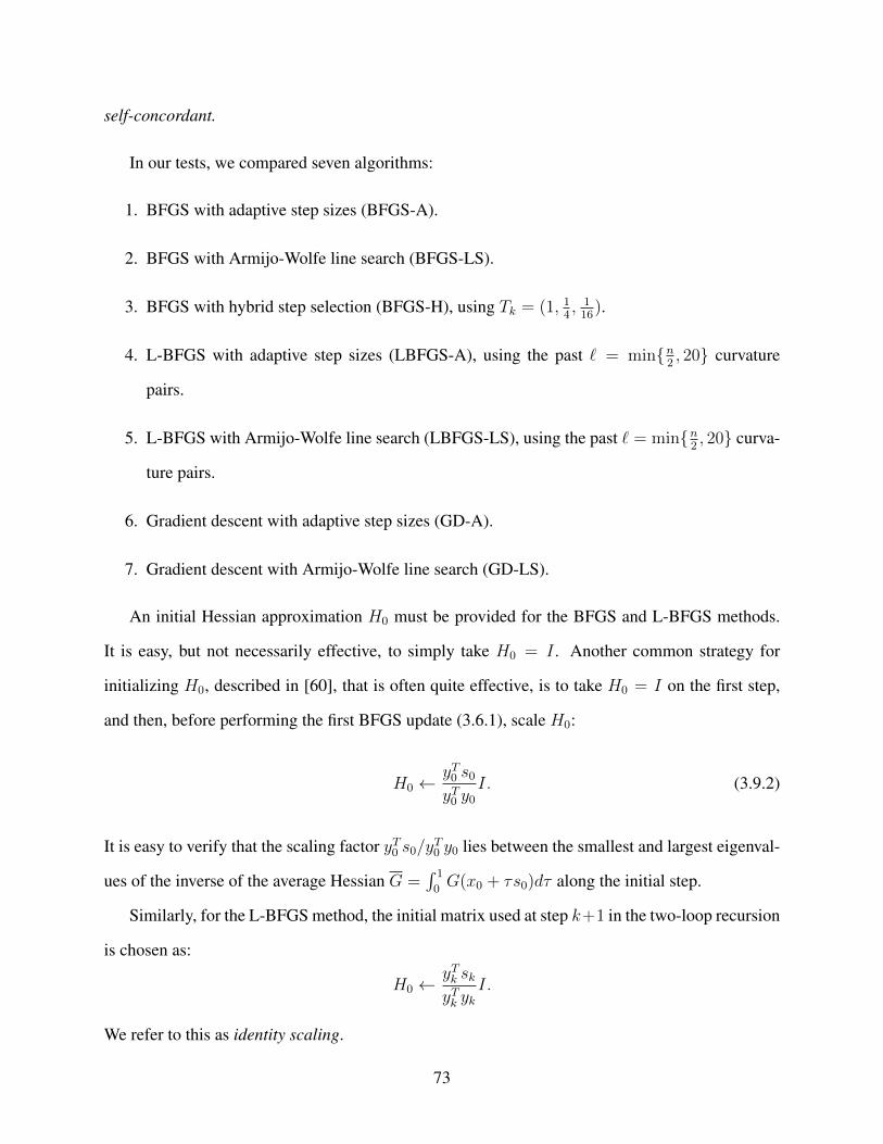
self-concordant.
In our tests, we compared seven algorithms:
1. BFGS with adaptive step sizes (BFGS-A).
2. BFGS with Armijo-Wolfe line search (BFGS-LS).
3. BFGS with hybrid step selection (BFGS-H), using Tk = (1, 14, 1
16).
4. L-BFGS with adaptive step sizes (LBFGS-A), using the past ` = minn2, 20 curvature
pairs.
5. L-BFGS with Armijo-Wolfe line search (LBFGS-LS), using the past ` = minn2, 20 curva-
ture pairs.
6. Gradient descent with adaptive step sizes (GD-A).
7. Gradient descent with Armijo-Wolfe line search (GD-LS).
An initial Hessian approximation H0 must be provided for the BFGS and L-BFGS methods.
It is easy, but not necessarily effective, to simply take H0 = I . Another common strategy for
initializing H0, described in [60], that is often quite effective, is to take H0 = I on the first step,
and then, before performing the first BFGS update (3.6.1), scale H0:
H0 ←yT0 s0
yT0 y0
I. (3.9.2)
It is easy to verify that the scaling factor yT0 s0/yT0 y0 lies between the smallest and largest eigenval-
ues of the inverse of the average Hessian G =∫ 1
0G(x0 + τs0)dτ along the initial step.
Similarly, for the L-BFGS method, the initial matrix used at step k+1 in the two-loop recursion
is chosen as:
H0 ←yTk skyTk yk
I.
We refer to this as identity scaling.
73
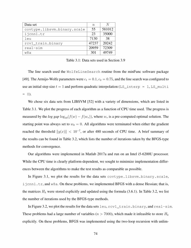
Data set n Ncovtype.libsvm.binary.scale 55 581012ijcnn1.tr 23 35000leu 7130 38rcv1_train.binary 47237 20242real-sim 20959 72309w8a 301 49749
Table 3.1: Data sets used in Section 3.9
The line search used the WolfeLineSearch routine from the minFunc software package
[49]. The Armijo-Wolfe parameters were c1 = 0.1, c2 = 0.75, and the line search was configured to
use an initial step size t = 1 and perform quadratic interpolation (LS_interp = 1, LS_multi
= 0).
We chose six data sets from LIBSVM [52] with a variety of dimensions, which are listed in
Table 3.1. We plot the progress of each algorithm as a function of CPU time used. The progress is
measured by the log gap log10(f(w)− f(w∗)), where w∗ is a pre-computed optimal solution. The
starting point was always set to w0 = 0. All algorithms were terminated when either the gradient
reached the threshold ‖g(x)‖ < 10−7, or after 480 seconds of CPU time. A brief summary of
the results can be found in Table 3.2, which lists the number of iterations taken by the BFGS-type
methods for convergence.
Our algorithms were implemented in Matlab 2017a and run on an Intel i5-6200U processor.
While the CPU time is clearly platform-dependent, we sought to minimize implementation differ-
ences between the algorithms to make the test results as comparable as possible.
In Figure 3.1, we plot the results for the data sets covtype.libsvm.binary.scale,
ijcnn1.tr, and w8a. On these problems, we implemented BFGS with a dense Hessian; that is,
the matrices Hk were stored explicitly and updated using the formula (3.6.1). In Table 3.2, we list
the number of iterations used by the BFGS-type methods.
In Figure 3.2, we plot the results for the data sets leu, rcv1_train.binary, and real-sim.
These problems had a large number of variables (n > 7000), which made it infeasible to store Hk
explicitly. On these problems, BFGS was implemented using the two-loop recursion with unlim-
74
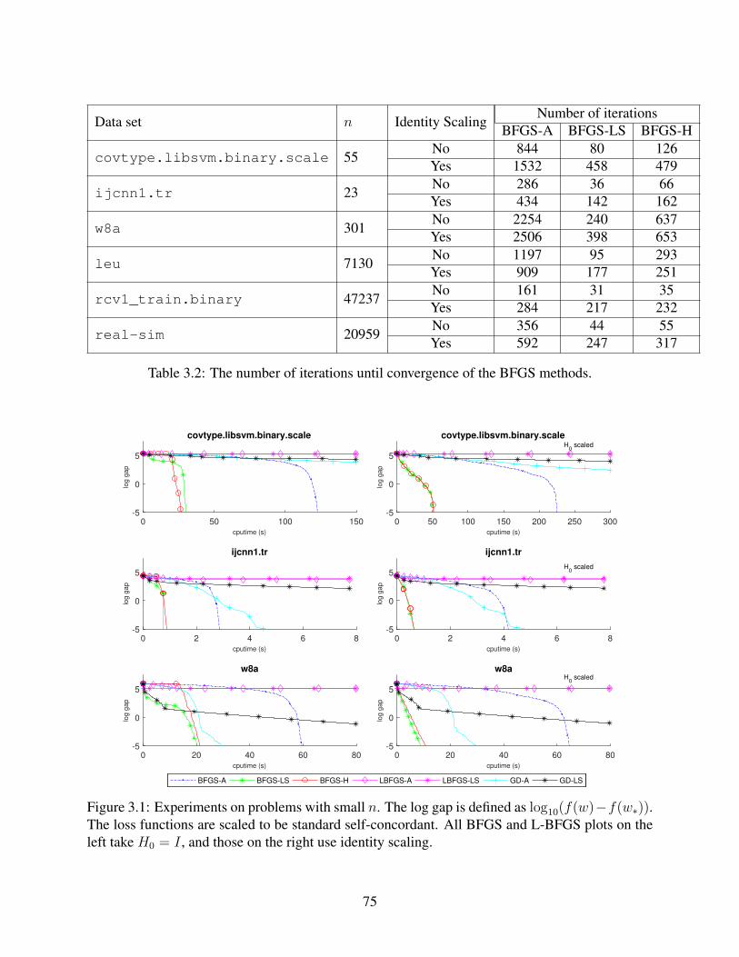
Data set n Identity ScalingNumber of iterations
BFGS-A BFGS-LS BFGS-H
covtype.libsvm.binary.scale 55No 844 80 126Yes 1532 458 479
ijcnn1.tr 23No 286 36 66Yes 434 142 162
w8a 301No 2254 240 637Yes 2506 398 653
leu 7130No 1197 95 293Yes 909 177 251
rcv1_train.binary 47237No 161 31 35Yes 284 217 232
real-sim 20959No 356 44 55Yes 592 247 317
Table 3.2: The number of iterations until convergence of the BFGS methods.
0 50 100 150cputime (s)
-5
0
5
log g
ap
covtype.libsvm.binary.scale
BFGS-A BFGS-LS BFGS-H LBFGS-A LBFGS-LS GD-A GD-LS
0 50 100 150 200 250 300cputime (s)
-5
0
5
log g
ap
covtype.libsvm.binary.scale
BFGS-A BFGS-LS BFGS-H LBFGS-A LBFGS-LS GD-A GD-LS
0 2 4 6 8cputime (s)
-5
0
5
log g
ap
ijcnn1.tr
BFGS-A BFGS-LS BFGS-H LBFGS-A LBFGS-LS GD-A GD-LS
0 2 4 6 8cputime (s)
-5
0
5
log g
ap
ijcnn1.tr
BFGS-A BFGS-LS BFGS-H LBFGS-A LBFGS-LS GD-A GD-LS
0 20 40 60 80cputime (s)
-5
0
5
log g
ap
w8a
BFGS-A BFGS-LS BFGS-H LBFGS-A LBFGS-LS GD-A GD-LS
0 20 40 60 80cputime (s)
-5
0
5
log g
ap
w8a
BFGS-A BFGS-LS BFGS-H LBFGS-A LBFGS-LS GD-A GD-LS
H0 scaled
H0 scaled
H0 scaled
Figure 3.1: Experiments on problems with small n. The log gap is defined as log10(f(w)−f(w∗)).The loss functions are scaled to be standard self-concordant. All BFGS and L-BFGS plots on theleft take H0 = I , and those on the right use identity scaling.
75
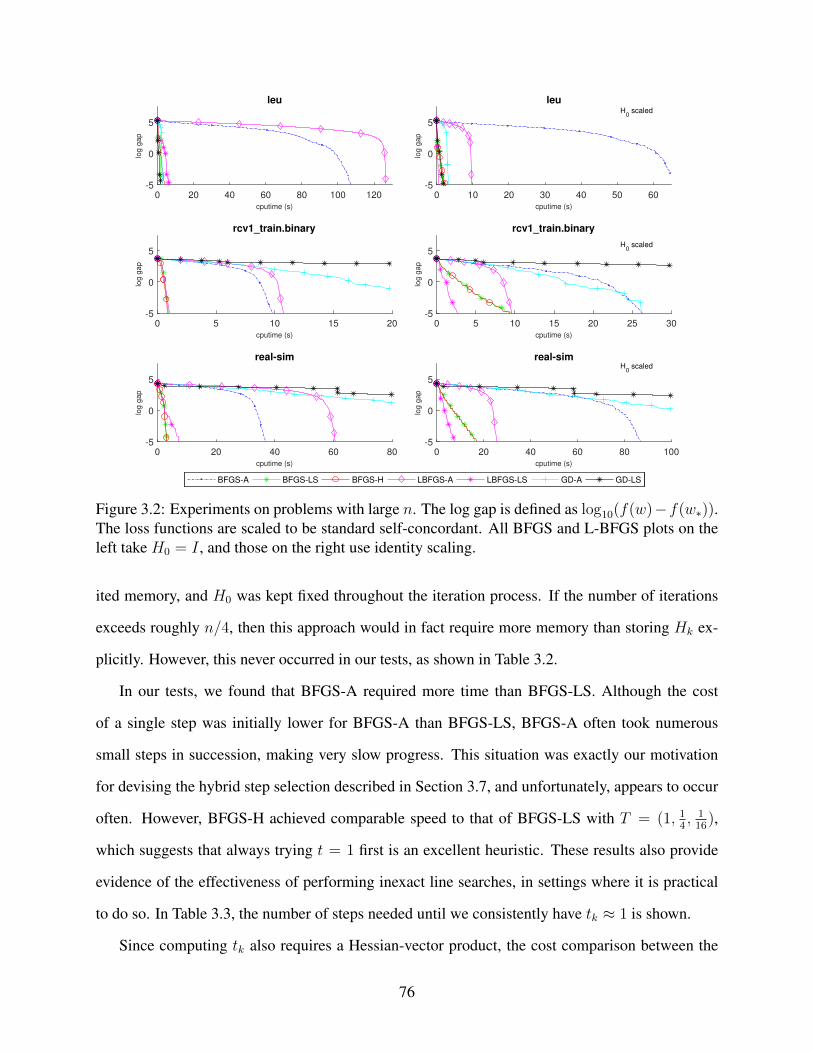
0 20 40 60 80 100 120cputime (s)
-5
0
5
log g
ap
leu
BFGS-A BFGS-LS BFGS-H LBFGS-A LBFGS-LS GD-A GD-LS
0 10 20 30 40 50 60cputime (s)
-5
0
5
log g
ap
leu
BFGS-A BFGS-LS BFGS-H LBFGS-A LBFGS-LS GD-A GD-LS
0 5 10 15 20cputime (s)
-5
0
5
log g
ap
rcv1_train.binary
BFGS-A BFGS-LS BFGS-H LBFGS-A LBFGS-LS GD-A GD-LS
0 5 10 15 20 25 30cputime (s)
-5
0
5
log g
ap
rcv1_train.binary
BFGS-A BFGS-LS BFGS-H LBFGS-A LBFGS-LS GD-A GD-LS
0 20 40 60 80cputime (s)
-5
0
5
log g
ap
real-sim
BFGS-A BFGS-LS BFGS-H LBFGS-A LBFGS-LS GD-A GD-LS
0 20 40 60 80 100cputime (s)
-5
0
5
log g
ap
real-sim
BFGS-A BFGS-LS BFGS-H LBFGS-A LBFGS-LS GD-A GD-LS
H0 scaled
H0 scaled
H0 scaled
Figure 3.2: Experiments on problems with large n. The log gap is defined as log10(f(w)−f(w∗)).The loss functions are scaled to be standard self-concordant. All BFGS and L-BFGS plots on theleft take H0 = I , and those on the right use identity scaling.
ited memory, and H0 was kept fixed throughout the iteration process. If the number of iterations
exceeds roughly n/4, then this approach would in fact require more memory than storing Hk ex-
plicitly. However, this never occurred in our tests, as shown in Table 3.2.
In our tests, we found that BFGS-A required more time than BFGS-LS. Although the cost
of a single step was initially lower for BFGS-A than BFGS-LS, BFGS-A often took numerous
small steps in succession, making very slow progress. This situation was exactly our motivation
for devising the hybrid step selection described in Section 3.7, and unfortunately, appears to occur
often. However, BFGS-H achieved comparable speed to that of BFGS-LS with T = (1, 14, 1
16),
which suggests that always trying t = 1 first is an excellent heuristic. These results also provide
evidence of the effectiveness of performing inexact line searches, in settings where it is practical
to do so. In Table 3.3, the number of steps needed until we consistently have tk ≈ 1 is shown.
Since computing tk also requires a Hessian-vector product, the cost comparison between the
76
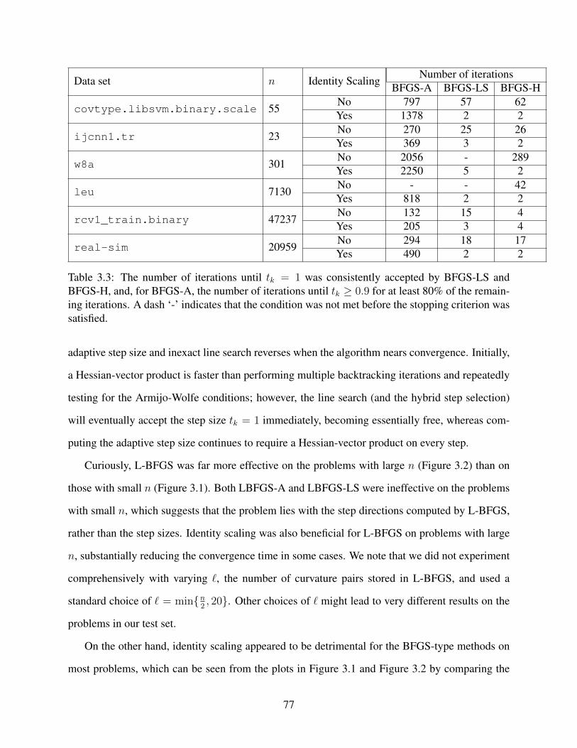
Data set n Identity ScalingNumber of iterations
BFGS-A BFGS-LS BFGS-H
covtype.libsvm.binary.scale 55No 797 57 62Yes 1378 2 2
ijcnn1.tr 23No 270 25 26Yes 369 3 2
w8a 301No 2056 - 289Yes 2250 5 2
leu 7130No - - 42Yes 818 2 2
rcv1_train.binary 47237No 132 15 4Yes 205 3 4
real-sim 20959No 294 18 17Yes 490 2 2
Table 3.3: The number of iterations until tk = 1 was consistently accepted by BFGS-LS andBFGS-H, and, for BFGS-A, the number of iterations until tk ≥ 0.9 for at least 80% of the remain-ing iterations. A dash ‘-’ indicates that the condition was not met before the stopping criterion wassatisfied.
adaptive step size and inexact line search reverses when the algorithm nears convergence. Initially,
a Hessian-vector product is faster than performing multiple backtracking iterations and repeatedly
testing for the Armijo-Wolfe conditions; however, the line search (and the hybrid step selection)
will eventually accept the step size tk = 1 immediately, becoming essentially free, whereas com-
puting the adaptive step size continues to require a Hessian-vector product on every step.
Curiously, L-BFGS was far more effective on the problems with large n (Figure 3.2) than on
those with small n (Figure 3.1). Both LBFGS-A and LBFGS-LS were ineffective on the problems
with small n, which suggests that the problem lies with the step directions computed by L-BFGS,
rather than the step sizes. Identity scaling was also beneficial for L-BFGS on problems with large
n, substantially reducing the convergence time in some cases. We note that we did not experiment
comprehensively with varying `, the number of curvature pairs stored in L-BFGS, and used a
standard choice of ` = minn2, 20. Other choices of ` might lead to very different results on the
problems in our test set.
On the other hand, identity scaling appeared to be detrimental for the BFGS-type methods on
most problems, which can be seen from the plots in Figure 3.1 and Figure 3.2 by comparing the
77
CPU time needed for convergence. For instance, on the data set covtype.libsvm.binary.scale,
the time to convergence for BFGS-A increased from 120s to 225s, and from 25s to 50s for BFGS-
LS and BFGS-H. In fact, identity scaling was beneficial for the BFGS-A method only on the data
set leu. The data set leu appears to be quite different from the other problems tested. The num-
ber of training samples for leu was m = 38, while for all other problems, m was at least 20,000.
Moreover, gradient descent with Armijo-Wolfe line search (GD-LS) was among the fastest meth-
ods on leu, while on the other test problems it was significantly outperformed by BFGS. The
iteration counts shown in Table 3.2 and Table 3.3 also indicate that identity scaling worsened
the performance of the BFGS methods on every problem except leu. Curiously, performing
identity scaling led to BFGS-H accepting tk = 1 at a much earlier iteration on all problems,
yet the total CPU time used by BFGS-H was longer for covtype.libsvm.binary.scale,
rcv1.train.binary, and real-sim.
GD-A was surprisingly effective, outperforming GD-LS on every problem except for leu.
This is somewhat surprising (in light of the performance of BFGS-A and BFGS-LS), and suggests
that the curvature-adaptive step size may be useful for selecting hyperparameters for first-order
methods.
3.9.2 Stochastic Methods
The experiments presented here are derived from the experiments in [62, §4]. Several stochastic
algorithms are tested on an online least-squares problem of the form
minw
E(Y −XTw)2 +1
2λ‖w‖2.
Online refers to the method of sampling: we can only access (X, Y ) by calling an oracle at each
iteration k, which returns |Sk| i.i.d instances of (X, Y ). The model for (X, Y ) has the following
specification:
• X has a multivariate normal distribution N(0,Σ), where Σ is the covariance matrix of the
78
w8a data set (see Table 3.1).
• Y = XTβ+ ε, where β is deterministic and sparse (80% sparsity) and ε ∼ N(0, 1) is a noise
component.
Since our model is based on the w8a data set, the dimension ofw is p = 300, and the regularizer
is set to λ = 1p.
We compare the following algorithms. For a deterministic method M , the corresponding
stochastic M method takes the step of the underlying M method, but computed from the em-
pirical objective function (3.8.2) sampled at each iteration. The convergence of these methods2 is
analyzed in [62]. In summary, the stochastic adaptive gradient descent method returns an ε-optimal
solution in expectation afterO(log(ε−1)) iterations when |Sk| is chosen as a constant (depending on
ε), and stochastic adaptive BFGS convergesR-superlinearly with probability 1 when |Sk| increases
superlinearly.
SBFGS-A The stochastic adaptive BFGS method. At each iteration, an adaptive BFGS step is
computed from the empirical objective function (3.8.2). The BFGS update is computed
from the pair (dk, Gkdk) which is more stable than using the pair (sk, yk) with the difference
yk of sampled gradients (see [32, 31]).
SBFGS-1 The stochastic BFGS method with constant step size α1. The step size α1 is given in
Table 3.4.
SN-A Nesterov’s stochastic damped Newton method [33].
SN-1 The stochastic Newton method with constant step size α1.
SGD-A Stochastic adaptive gradient descent.
SGD-i Stochastic gradient descent with constant step size αi for i = 1, . . . , 4 (Table 3.4).
2Note: the stochastic adaptive BFGS analyzed in [62] is slightly different, as it incorporates an additional Wolfecondition test.
79
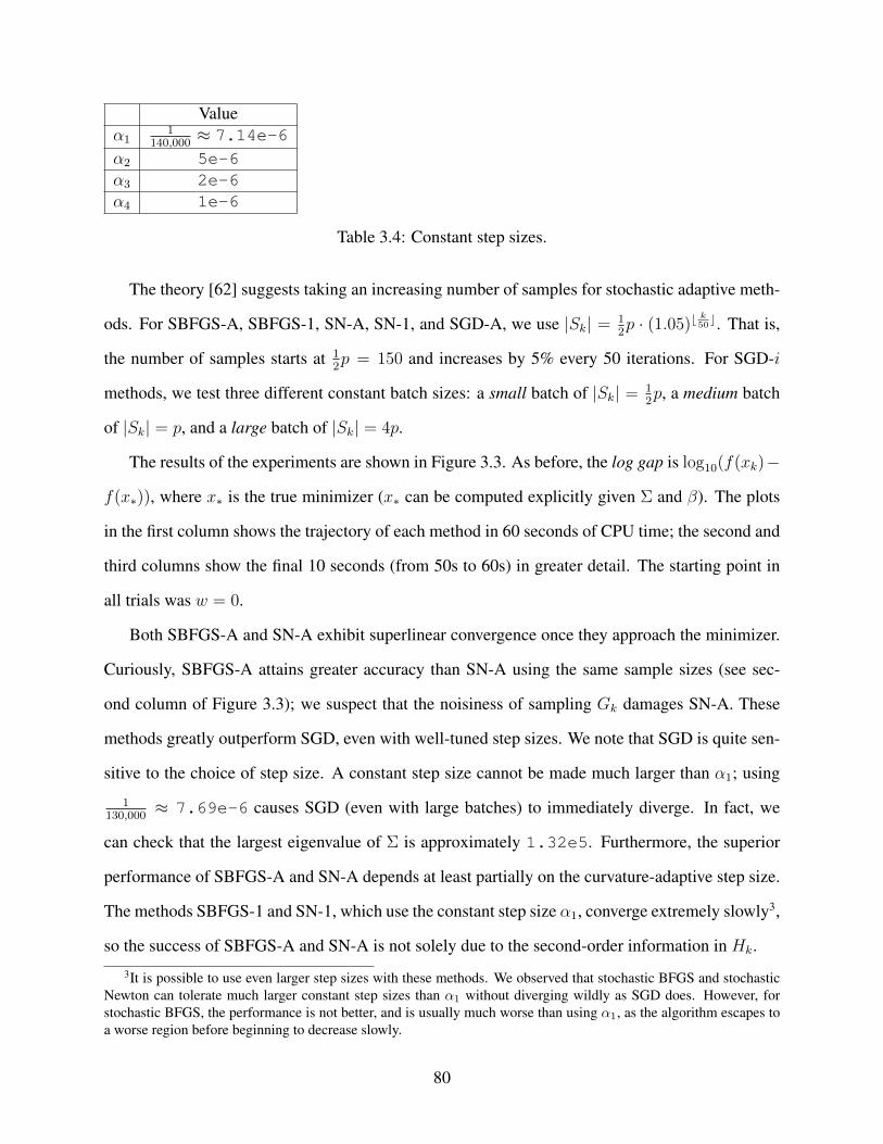
Valueα1
1140,000
≈ 7.14e-6
α2 5e-6α3 2e-6α4 1e-6
Table 3.4: Constant step sizes.
The theory [62] suggests taking an increasing number of samples for stochastic adaptive meth-
ods. For SBFGS-A, SBFGS-1, SN-A, SN-1, and SGD-A, we use |Sk| = 12p · (1.05)b
k50c. That is,
the number of samples starts at 12p = 150 and increases by 5% every 50 iterations. For SGD-i
methods, we test three different constant batch sizes: a small batch of |Sk| = 12p, a medium batch
of |Sk| = p, and a large batch of |Sk| = 4p.
The results of the experiments are shown in Figure 3.3. As before, the log gap is log10(f(xk)−
f(x∗)), where x∗ is the true minimizer (x∗ can be computed explicitly given Σ and β). The plots
in the first column shows the trajectory of each method in 60 seconds of CPU time; the second and
third columns show the final 10 seconds (from 50s to 60s) in greater detail. The starting point in
all trials was w = 0.
Both SBFGS-A and SN-A exhibit superlinear convergence once they approach the minimizer.
Curiously, SBFGS-A attains greater accuracy than SN-A using the same sample sizes (see sec-
ond column of Figure 3.3); we suspect that the noisiness of sampling Gk damages SN-A. These
methods greatly outperform SGD, even with well-tuned step sizes. We note that SGD is quite sen-
sitive to the choice of step size. A constant step size cannot be made much larger than α1; using
1130,000
≈ 7.69e-6 causes SGD (even with large batches) to immediately diverge. In fact, we
can check that the largest eigenvalue of Σ is approximately 1.32e5. Furthermore, the superior
performance of SBFGS-A and SN-A depends at least partially on the curvature-adaptive step size.
The methods SBFGS-1 and SN-1, which use the constant step size α1, converge extremely slowly3,
so the success of SBFGS-A and SN-A is not solely due to the second-order information in Hk.
3It is possible to use even larger step sizes with these methods. We observed that stochastic BFGS and stochasticNewton can tolerate much larger constant step sizes than α1 without diverging wildly as SGD does. However, forstochastic BFGS, the performance is not better, and is usually much worse than using α1, as the algorithm escapes toa worse region before beginning to decrease slowly.
80
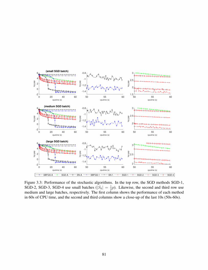
0 20 40 60cputime (s)
-2
0
2
4
6
log g
ap
(small SGD batch)
SBFGS-A SGD-A SN-A SBFGS-1 SN-1 SGD-1 SGD-2 SGD-3 SGD-4
0 20 40 60cputime (s)
-2
0
2
4
6
log g
ap
(medium SGD batch)
SBFGS-A SGD-A SN-A SBFGS-1 SN-1 SGD-1 SGD-2 SGD-3 SGD-4
0 20 40 60cputime (s)
-2
0
2
4
6
log g
ap
(large SGD batch)
SBFGS-A SGD-A SN-A SBFGS-1 SN-1 SGD-1 SGD-2 SGD-3 SGD-4
50 55 60cputime (s)
-1.4
-1.2
-1
-0.8
log g
ap
50 55 60cputime (s)
-1.4
-1.2
-1
-0.8
log g
ap
50 55 60cputime (s)
-1.4
-1.2
-1
-0.8
log g
ap
50 55 60cputime (s)
1.5
2
2.5
3
log g
ap
50 55 60cputime (s)
2
2.5
3
log g
ap
50 55 60cputime (s)
2
2.5
3
log g
ap
Figure 3.3: Performance of the stochastic algorithms. In the top row, the SGD methods SGD-1,SGD-2, SGD-3, SGD-4 use small batches (|Sk| = 1
2p). Likewise, the second and third row use
medium and large batches, respectively. The first column shows the performance of each methodin 60s of CPU time, and the second and third columns show a close-up of the last 10s (50s-60s).
81

SGD-A was slower than SGD with tuned step sizes. We found that the initial adaptive step
size was 1e-8, which explains the relatively slow convergence of SGD-A. It is also worth noting
that even with a small initial sample, SGD-A never produced an overly large step size causing it to
diverge or oscillate, something which is not strictly guaranteed by the theory.
We have not touched on the subject of variance reduction, which is generally crucial, though
not particularly relevant when considering the results in Figure 3.3. Good variance reduction tech-
niques will be important for designing an effective, general-purpose solver based on SBFGS-A,
SN-A, or indeed, any other of the stochastic algorithms tested.
82

Chapter 4: Distributed Optimization: The Leader Stochastic Gradient
Descent Algorithm
4.1 Introduction
The advent of increasingly large data and models has led to the use of parallel and distributed
computing for machine learning [36, 64]. A number of algorithms [65, 38, 66, 67] and systems
(DOWNPOUR, Horovod) [68, 69] have been proposed for specifically taking advantage of paral-
lelism. Consider again the loss function encountered in a typical supervised learning problem:
minxf(x) =
1
N
N∑i=1
`(x; ξi)
where bothN , the size of the training data ξ1, . . . , ξN, as well as the dimension d of the model pa-
rameters x, may be large. A straightforward way to parallelize the standard Stochastic Gradient De-
scent (SGD) algorithm is data parallelism: given p parallel workers, the minibatch B at each step
is partitioned into p sets B1, . . . , Bp, and each worker computes the gradient gj =∑ξi∈Bj
∇`(x; ξi).
A central coordinator then aggregates the gradients and computes the stochastic gradient∑p
j=1 gj
for SGD, performing an update and communicating new parameters x+ to the workers.
The data-parallel strategy is simple and easy to implement. However, it has two notable draw-
backs. The first is that it quickly encounters limits to parallelism. The limiting factor is the size
of the minibatch: a well-known empirical phenomenon is that generalization is often poor when
using SGD with large minibatches [70, 71]. This is not entirely understood, and is often attributed
to the flat minima theory, which hypothesizes that local minima belonging to ‘flatter’ regions of
the loss landscape result in better generalization. Algorithms have been proposed to modify SGD
to converge to such ‘flat’ minima [72, 73]. Another common strategy is to increase the step size
83

when using large minibatches [74, 37].
The second drawback of data parallelism is the frequency of communication. At every step,
each worker must communicate the gradient of its assigned subset to the central coordinator, and
the coordinator then must communicate updated parameters to every worker. Though these op-
erations have efficient implementations and are specifically supported by computing frameworks
such as MPI (via the reduce and scatter operations), requiring synchronization between all work-
ers and the coordinator can lead to significant and unpredictable communication delays in practice.
Allowing less strict synchronization leads to ‘asynchronous’ algorithms which have convergence
guarantees under various assumptions on the delay [75, 76], it is still often unclear whether such
delay models are realistic or whether good performance is obtained in practice.
In a data-parallel algorithm, there is a single set of model parameters shared by all the work-
ers at each step. Another paradigm for distributed optimization allows for multiple independent
instances of the parameters being separately optimized. Unlike data-parallel algorithms, these
algorithms can allow for reduced communication, because we do not require that the separate in-
stances of the model share weights at every point in time. A key algorithm of this type is Elastic
Averaging SGD [38, 77], which uses an L2-penalty to enforce a ‘soft’ consensus between the mod-
els on separate workers. To specify this algorithm, assume that we have p independent workers,
each having its own copy x(i) of the parameters, and let f(·) denote the common objective func-
tion. In the machine learning context, note that f denotes the total loss f(x) = 1N
∑Ni=1 `(x; ξi) –
we assume each worker to have access to the same training dataset ξ1, . . . , ξN. Finally, let x be
another decision variable, which we call the consensus variable. Each worker performs the update
x(i)k+1 = x
(i)k − η(∇f(x
(i)k ) + λ(x
(i)k − xk)).
It is not hard to see that this corresponds to performing a gradient descent step with respect to x(i)
for the loss function
f(x) +λ
2‖x− x‖2.
84

In the stochastic case (for SGD instead of GD), the gradient ∇f(x(i)) is replaced by a stochastic
gradient estimate. In parallel to the workers updating their parameters x(i)k , the consensus variable
in EASGD is updated by a moving average of the model parameters:
xk+1 = (1− β)xk + β
(1
p
p∑i=1
x(i)k
)
In practice, we can reduce communication by performing multiple gradient steps for each set
of parameters x(i), and either holding the consensus variable xk fixed to its value at step k, or
including the consensus term λ(x(i)k − xk) only for the very first step. Since each worker can
perform SGD independently for f(x(i)), the only communication is a periodic gather operation to
average the worker parameters. This variant is called the Asynchronous EASGD.
EASGD has been successfully applied to deep learning [38], and is widely used in industry1.
It is interesting that EASGD has proven to be effective for deep learning, a problem domain where
the loss function is typically highly nonconvex, while the known convergence analysis only applies
to convex problems. In fact, we can show that for nonconvex problems, EASGD has stationary
points which are “spurious” in the sense of not corresponding to stationary points of the underlying
objective function f .
Proposition 4.1.1. Let p = 2. There exists a Lipschitz differentiable function f : R→ R such that
for every 0 < λ ≤ 1, there exists a point (xλ, yλ, 0) which is a stationary point of EASGD with
parameter λ, but none of xλ, yλ, 0 is a stationary point of f .
We prove this proposition in the next section.
To see how this can theoretical pitfall can impact convergence, observe that on nonconvex
problems, the workers x(i) may converge towards different local minima, causing the consensus
variable (which converges to the average of the worker parameters) to pull the workers in the
wrong direction. In particular, when the objective landscape is symmetric, the consensus variable
can become permanently trapped at a local maximum in between the local minima. Symmetry
1Personal communication.
85
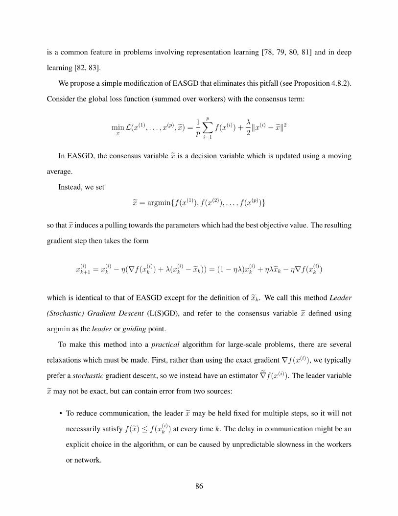
is a common feature in problems involving representation learning [78, 79, 80, 81] and in deep
learning [82, 83].
We propose a simple modification of EASGD that eliminates this pitfall (see Proposition 4.8.2).
Consider the global loss function (summed over workers) with the consensus term:
minxL(x(1), . . . , x(p), x) =
1
p
p∑i=1
f(x(i)) +λ
2‖x(i) − x‖2
In EASGD, the consensus variable x is a decision variable which is updated using a moving
average.
Instead, we set
x = argminf(x(1)), f(x(2)), . . . , f(x(p))
so that x induces a pulling towards the parameters which had the best objective value. The resulting
gradient step then takes the form
x(i)k+1 = x
(i)k − η(∇f(x
(i)k ) + λ(x
(i)k − xk)) = (1− ηλ)x
(i)k + ηλxk − η∇f(x
(i)k )
which is identical to that of EASGD except for the definition of xk. We call this method Leader
(Stochastic) Gradient Descent (L(S)GD), and refer to the consensus variable x defined using
argmin as the leader or guiding point.
To make this method into a practical algorithm for large-scale problems, there are several
relaxations which must be made. First, rather than using the exact gradient ∇f(x(i)), we typically
prefer a stochastic gradient descent, so we instead have an estimator ∇f(x(i)). The leader variable
x may not be exact, but can contain error from two sources:
• To reduce communication, the leader x may be held fixed for multiple steps, so it will not
necessarily satisfy f(x) ≤ f(x(i)k ) at every time k. The delay in communication might be an
explicit choice in the algorithm, or can be caused by unpredictable slowness in the workers
or network.
86
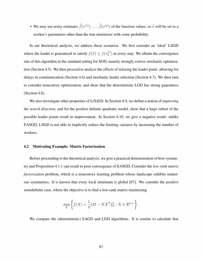
• We may use noisy estimates f(x(1)), . . . , f(x(p)) of the function values, so x will be set to a
worker’s parameters other than the true minimizer with some probability.
In our theoretical analysis, we address these scenarios. We first consider an ‘ideal’ LSGD
where the leader is guaranteed to satisfy f(x) ≤ f(x(i)k ) at every step. We obtain the convergence
rate of this algorithm in the standard setting for SGD, namely strongly convex stochastic optimiza-
tion (Section 4.5). We then proceed to analyze the effects of relaxing the leader point: allowing for
delays in communication (Section 4.6) and stochastic leader selection (Section 4.7). We then turn
to consider nonconvex optimization, and show that the deterministic LGD has strong guarantees
(Section 4.8).
We also investigate other properties of L(S)GD. In Section 4.9, we define a notion of improving
the search direction, and for the positive definite quadratic model, show that a large subset of the
possible leader points result in improvement. In Section 4.10, we give a negative result: unlike
EASGD, LSGD is not able to implicitly reduce the limiting variance by increasing the number of
workers.
4.2 Motivating Example: Matrix Factorization
Before proceeding to the theoretical analysis, we give a practical demonstration of how symme-
try and Proposition 4.1.1 can result in poor convergence of EASGD. Consider the low-rank matrix
factorization problem, which is a nonconvex learning problem whose landscape exhibits numer-
ous symmetries. It is known that every local minimum is global [67]. We consider the positive
semidefinite case, where the objective is to find a low-rank matrix minimizing
minX
f(X) =
1
4‖M −XXT‖2
F : X ∈ Rd×r.
We compare the (deterministic) EAGD and LGD algorithms. It is routine to calculate that
87
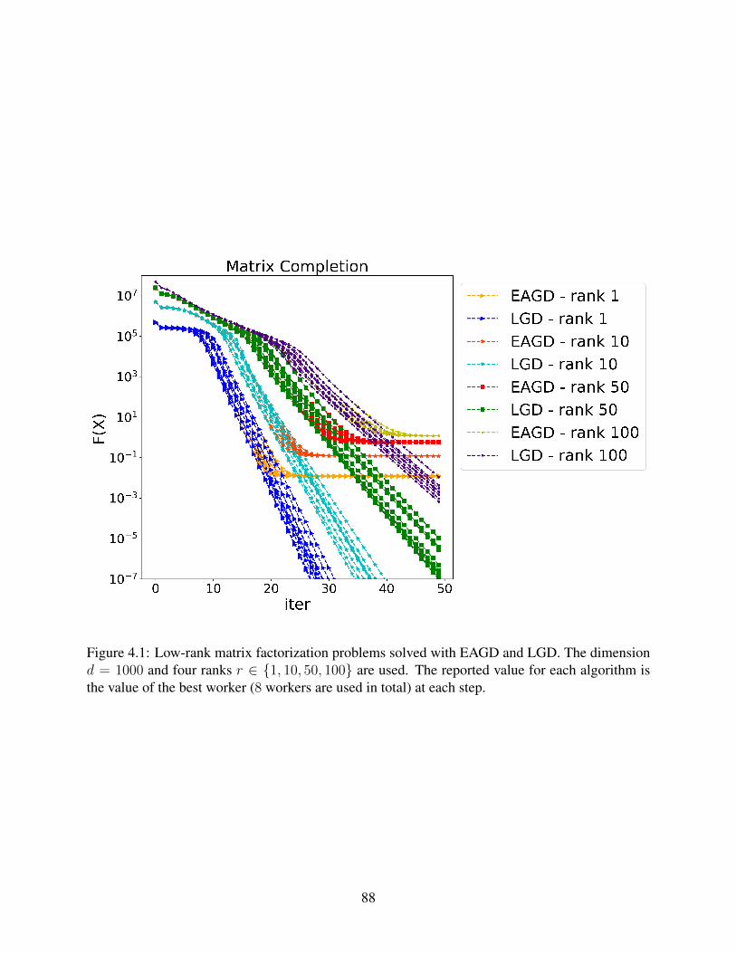
Figure 4.1: Low-rank matrix factorization problems solved with EAGD and LGD. The dimensiond = 1000 and four ranks r ∈ 1, 10, 50, 100 are used. The reported value for each algorithm isthe value of the best worker (8 workers are used in total) at each step.
88

∇F (X) = (XXT −M)X . The EASGD and LSGD updates for X can be expressed as
X+ = (1− ηλ)X + ηλZ − η∇F (X).
For EASGD, Z = X , and X is updated by
X+ = (1− pηλ)X + pηλ
(1
p
p∑i=1
X i
).
For LSGD, Z = argminF (X1), . . . , F (Xp), and is updated at the beginning of every step.
For four choices of the rank r, we generated 10 random instances of the matrix completion
problem, and solved each with EAGD and LGD, initialized from the same starting points (we use
8 workers). For each algorithm, we report the progress of the best objective value at each iteration,
over all workers. Figure 4.1 shows the results across 10 random experiments for each rank.
It is clear that EAGD slows down significantly as it approaches a minimizer. Typically, the
center X of EAGD is close to the average of the workers, which is a poor solution for the matrix
completion problem when the workers are approaching different local minimizers, even though all
local minimizers are globally optimal. This induces a pull on each node away from the minimizers,
which makes it extremely difficult for EAGD to attain a solution of high accuracy. In comparison,
LGD does not have this issue.
4.3 Definitions and Preliminaries
Throughout our proofs in this section, we will often consider a more general form of the al-
gorithm where the consensus variable is replaced by an arbitrary point z. That is, we optimize
L(x(1), . . . , x(p)) =1
p
p∑i=1
f(x(i)) +λ
2‖x(i) − z‖2 (4.3.1)
where z may be given by weaker properties.
A L(S)GD step (with respect to a given z) is a (stochastic) gradient step applied to L: writing
89
z = x at a particular (x(1), . . . , x(p)), the step in the variable x(i) is
η(∇f(x(i)) + λ(x(i) − z)).
The deterministic LGD algorithm uses the exact gradient ∇f(x(i)) = ∇f(x(i)), and the stochastic
LSGD algorithm samples an unbiased estimator with E[∇f(x(i))] = ∇f(x(i)). This estimator is
assumed to satisfy standard growth conditions on its variance, which are given in the analysis.
Observe that if z is defined as the standard LSGD point argminf(x(1), . . . , x(p), then for the
index i such that z = x(i), the step for x(i) reduces to a gradient step.
To reduce communication costs in the distributed setting, we may choose to infrequently update
the leader. For each time k, the variable x(i) will take bi(k) L(S)GD steps, using the same leader
fixed from the beginning (alternately, we compare the leader with the function value of x(i) only).
This number bi(k) is the communication period. Typically, bi(k) is constant for all workers i and
all steps k, and we simply write τ for the communication period.
After each variable takes its bi(k) steps, the function values are computed and the next leader
is detremined. Let x(k) denote the leader for the k-th period, and let x(i)k,j denote the value of the
variable x(i) after taking j steps in the period k.
In practice, we may use multiple leaders to increase locality and reduce communication costs,
such as in the group method described in [3]. This arises because of natural clustering in the
hardware, and heterogeneity in communication costs. For example, a standard setup consists of
multiple machines for which communication is expensive, but with each machine having multiple
GPUs internally for which data transfer is fast between GPUs. For our theory, it suffices to consider
having only one leader. The formulation with multiple leaders (for one variable) is given by
minxf(x) +
λ1
2‖x− z1‖2 + . . .+
λc2‖x− zc‖2
However, this is equivalent to minimizing f(x) + Λ2‖x − z‖2, where Λ =
∑ci=1 λi and z =
1Λ
∑ci=1 λizi. Thus, for our theoretical analysis, we may reduce to the case of a single leader.
90
4.4 Stationary Points of EASGD
We first prove Proposition 4.1.1, which shows that EASGD can converge to spurious stationary
points when the objective function is nonconvex.
Proposition. Let p = 2. There exists a Lipschitz differentiable function f : R → R such that
for every 0 < λ ≤ 1, there exists a point (xλ, yλ, 0) which is a stationary point of EASGD with
parameter λ, but none of xλ, yλ, 0 is a stationary point of f .
Proof. Define f(x) by
f(x) =
ex+1 if x < −1
q(x) if − 1 ≤ x ≤ 1
e−x+1 if x > 1
where q(x) = a6x6 + . . . + a1x + a0 is a sixth-degree polynomial. For f to be Lipschitz dif-
ferentiable, we will select q(x) to make f twice continuously differentiable, with bounded sec-
ond derivative. To make f twice continuously differentiable, we must have q(1) = 1, q′(1) =
−1, q′′(1) = 1 and q(−1) = −1, q′(−1) = 1, q′′(−1) = −1. Since we aim to have f ′(0) 6= 0, we
also will require f ′(0) = q′(0) = 1. The existence of q is equivalent to the solvability of the linear
system
1 1 1 1 1 1 1
1 −1 1 −1 1 −1 1
6 5 4 3 2 1 0
6 −5 4 −3 2 −1 0
30 20 12 6 2 0 0
30 −20 12 −6 2 0 0
0 0 0 0 0 0 1
a6
a5
a4
a3
a2
a1
a0
=
1
−1
−1
1
1
−1
1
which is easily seen to be solvable. Thus, we deduce that such a function f exists.
Suppose that we have two workers, and write x = x(1), y = x(2). Assume also that we have
exact gradients (so the problem is deterministic). It remains to show that for any 0 < λ ≤ 1,
91
there exists a stationary point (x, y, 0) of EASGD. When the consensus variable satisfies x = 0,
the first-order condition for x yields f ′(x) + λx = 0. Since λ ≤ 1, we have λ(1) + f ′(1) ≤ 0.
For x ≥ 1, f ′(x) = −e−x+1 is an increasing function, so f ′(x) + λx is increasing, and we deduce
that there exists a solution yλ ≥ 1 with λyλ + f ′(yλ) = 0. By symmetry, −yλ ≤ −1 satisfies
f ′(−yλ) + λ(−yλ) = 0, since f ′(x) = ex+1 for x ≤ −1.
Since xλ = −yλ, the EASGD update of the consensus variable yields
x+ = (1− β)x+β
2(xλ + yλ)
= (1− β)x = 0
Hence, (−yλ, yλ, 0) is a stationary point of EASGD, but none of −yλ, yλ, 0 are stationary
points of f .
4.5 Convergence Rates for Stochastic Convex Optimization
Our key technical result is that LSGD satisfies a similar one-step descent in expectation as
SGD, with an additional term corresponding to the pull of the leader. To provide a unified analysis
of ‘pure’ LSGD as well as more practical variants where the leader is updated infrequently or with
errors, we consider a general iteration x+ = x−η(g(x)+λ(x−z)), where z is an arbitrary guiding
point; that is, z may not be the minimizer of x(1), . . . , x(p), nor even satisfy f(z) ≤ f(x(i)). Since
the nodes operate independently except when updating z, we may analyze LSGD steps for each
node individually, and we write x = x(i) for brevity.
Assumption 1 f is M -Lipschitz-differentiable and m-strongly convex, which is to say, the gradi-
ent ∇f satisfies ‖∇f(x)−∇f(y)‖ ≤M‖x− y‖, and f satisfies
f(y) ≥ f(x) +∇f(x)T (y − x) +m
2‖y − x‖2.
We write x∗ for the unique minimizer of f , and κ := Mm
for the condition number of f .
92
Lemma 4.5.1 (One-Step Descent). Let f satisfy Assumption 1, and let g(x) be an unbiased esti-
mator for∇f(x) with variance Var(g(x)) ≤ σ2 + ν‖∇f(x)‖2.
Fix an initial point x, and let z be another point, with δ := x− z. We take a LSGD step
x+ = x− η(g(x) + λ(x− z)).
Then each step of LSGD satisfies:
Ef(x+) ≤ f(x)− η
2(1− ηM(ν + 1))‖∇f(x)‖2 (4.5.1)
− η
4λ(m− 2ηMλ)‖δ‖2
− η√λ√2
(√m− ηM
√2λ)‖∇f(x)‖‖δ‖
− ηλ(f(x)− f(z)) +η2
2Mσ2
Hence, for sufficiently small η, λ with η ≤ (2M(ν + 1))−1 and ηλ ≤ (2κ)−1, η√λ ≤ (κ
√2m)−1,
we have
Ef(x+)− f(x∗) ≤ (1−mη)(f(x)− f(x∗))− ηλ(f(x)− f(z)) +η2M
2σ2 (4.5.2)
Proof. The proof is similar to the convergence analysis of SGD. We take a Taylor expansion at the
point x:
f(x+) = f(x)− η∇f(x)T (g(x) + λδ) +η2
2(g(x) + λδ)TG(g(x) + λδ)
whereG = ∇2f(x′) for some x′ between x, x+. Taking the expectation and using Eg(x) = ∇f(x),
Ef(x+) = f(x)− η‖∇f(x)‖2 − ηλ∇f(x)T δ +η2λ2
2δTGδ + η2λ∇f(x)TGδ +
η2
2E[g(x)TGg(x)]
93
Taking another Taylor expansion along the direction −δ, observe that
f(z) = f(x)−∇f(x)T δ +1
2δT Gδ ≥ f(x)−∇f(x)T δ +
m
2‖δ‖2
from which we deduce that −∇f(x)T δ ≤ −(f(x)− f(z) + m2‖δ‖2). Substituting this above, and
splitting both the terms η‖∇f(x)‖2, η2mλ‖δ‖2 in half, we obtain
Ef(x+) = f(x)− η
2‖∇f(x)‖2 +
η2
2E[g(x)TGg(x)]
− η
4mλ‖δ‖2 +
η2
2λ2δTGδ
− η
2‖∇f(x)‖2 − η
4mλ‖δ‖2 + η2λ∇f(x)TGδ
− ηλ(f(x)− f(z))
We proceed to bound each line. For the first line, the standard bias-variance decomposition
yields
E[g(x)TGg(x)] ≤ME‖g(x)‖2 ≤M((ν + 1)‖∇f(x)‖2 + σ2)
and so
−η2‖∇f(x)‖2 +
η2
2E[g(x)TGg(x)] ≤ −η
2(1− ηM(ν + 1))‖∇f(x)‖2 +
η2
2Mσ2
For the second line, using G MI again, we have η2
2λ2δTGδ ≤ η2M
2λ2‖δ‖2. Hence,
−η4mλ‖δ‖2 +
η2
2λ2δTGδ ≤ −η
4λ(m− 2ηMλ)‖δ‖2
For the third line, we apply the inequality a2 + b2 ≥ 2ab to obtain
η
2‖∇f(x)‖2 +
η
4mλ‖δ‖2 ≥ η√
2
√mλ‖∇f(x)‖‖δ‖
On the other hand, the Cauchy-Schwarz inequality yields ∇f(x)TGδ = (G1/2∇f(x))T (G1/2δ) ≤
94
M‖∇f(x)‖‖δ‖. Hence
−η2‖∇f(x)‖2 − η
4mλ‖δ‖2 + η2λ∇f(x)TGδ ≤ −η
√λ√2
(√m− ηM
√2λ)‖∇f(x)‖‖δ‖
Combining these inequalities yields the desired result.
From this result, we can then demonstrate a sublinear convergence rate for LSGD, which holds
whenever the leader is chosen so that its value is lower than the other workers.
Theorem 4.5.2. Let f satisfy Assumption 1. Suppose that the leader zk is always chosen so that
f(zk) ≤ f(xk). If η, λ are fixed so that η ≤ (2M(ν+ 1))−1 and ηλ ≤ (2κ)−1, η√λ ≤ (κ
√2m)−1,
then
lim supk→∞
Ef(xk)− f(x∗) ≤ 1
2ηκσ2.
If η decreases at the rate ηk = Θ( 1k), then Ef(xk)− f(x∗) = O( 1
k).
Proof. This result follows (4.5.2) and Theorems 4.6 and 4.7 of [17].
The O( 1k) rate of LSGD matches that of comparable distributed methods. Both Hogwild [65]
and EASGD achieve a rate of O( 1k) on strongly convex objective functions. We note that conver-
gence rates have not been analyzed for many distributed algorithms (including DOWNPOUR [68]
and Parle [66]).
One may ask whether LSGD may surpass the 1k
sublinear convergence rate on strongly concex
functions. However, the Ω( 1k) lower bound obtained in [84] also applies to LSGD, since we may
view each LSGD iteration as making p calls to a stochastic first-order oracle.
4.6 Stochastic Convex Optimization with Communication Delay
In practice, communication between distributed machines is costly. The LSGD algorithm has a
communication period τ for which the leader is only updated every τ iterations, so each node can
run independently during that period. This τ is allowed to differ between nodes, and over time,
95
which captures the asynchronous and multi-leader variants of LSGD. We write xk,j for the j-th step
during the k-th period. It may occur that f(z) > f(xk,j) for some k, j, that is, the current solution
xk,j is now better than the last selected leader. In this case, the leader term λ(x− z) may no longer
be beneficial, and instead simply pulls x toward z. There is no general way to determine how many
steps are taken before this event. However, once f(x) ≤ f(z), we can show that subsequent LSGD
steps will not make the solution worse than the stale leader z, up to gradient noise. This is captured
by the following corollary:
Corollary 4.6.1. If f(x) ≤ f(z), then
Ef(x+) ≤ f(z) +η2
2Mσ2
− η
2(1− ηM(ν + 1))‖∇f(x)‖2 − η
4λ(m− 2ηMλ)‖δ‖2
− η√λ√2
(√m− ηM
√2λ)‖∇f(x)‖‖δ‖
Proof. Follows from Lemma 4.5.1.
Corollary 4.6.2. In the deterministic case, once we reach a point with f(x) ≤ f(z), then f(x+) ≤
f(z) as well.
Suppose we simply continue to run the LSGD algorithm with fixed z. As τ goes to infinity,
LSGD converges to the minimizer of ψ(x) = f(x) + λ2‖x− z‖2, which is quantifiably better than
z as captured in Lemma 4.6.3. Together, these facts show that LSGD is safe to use with long
communication periods as long as the original leader is good.
Lemma 4.6.3. Let f be twice differentiable and strongly convex, with mI ∇2f(x) for m > 0,
and let x∗ be the minimizer of f . Fix a constant λ and any point z, and define the function ψ(x) =
f(x) + λ2‖x − z‖2. Since ψ is strongly convex, it has a unique minimizer w. The minimizer w
satisfies2
f(w)− f(x∗) ≤ λ
m+ λ(f(z)− f(x∗)) (4.6.1)
2If we also assume that f is Lipschitz differentiable (that is,∇2f(x) MI), then we can obtain a similar inequalityto the second directly from the first, but this is generally weaker than the bound given here.
96

and
‖w − x∗‖2 ≤ λ2
m(m+ λ)‖z − x∗‖2 (4.6.2)
Proof. The first-order condition for w implies that ∇f(w) + λ(w − z) = 0, so λ2‖w − z‖2 =
‖∇f(w)‖2. Combining this with the Polyak-Łojasiewicz inequality, we obtain
λ
2‖w − z‖2 =
1
2λ‖∇f(w)‖2 ≥ m
λ(f(w)− f(x∗))
We have ψ(w) ≤ ψ(z) = f(z), so f(w) − f(x∗) ≤ f(z) − f(x∗) − λ2‖w − z‖2. Substituting,
f(w)− f(x∗) ≤ f(z)− f(x∗)− mλ
(f(w)− f(x∗)), which yields the first inequality.
We also have ψ(w) = f(w) + λ2‖w − z‖2 ≤ ψ(x∗) = f(x∗) + λ
2‖x∗ − z‖2, whence f(w) −
f(x∗) ≤ λ2(‖x∗ − z‖2 − ‖w − z‖2). Hence, we have
f(w)− f(x∗) ≤ λ
2(‖x∗ − z‖2 − ‖w − z‖2)
≤ λ
2‖z − x∗‖2 − m
λ(f(w)− f(x∗))
so f(w) − f(x∗) ≤ λ2
2(m+λ)‖z − x∗‖2. Finally, f(w) − f(x∗) ≥ m
2‖w − x∗‖2, which yields the
result.
The theoretical results here and in Section 4.5 address two fundamental instances of the LSGD
algorithm: the ‘synchronous’ case where communication occurs each round, and the ‘infinitely
asynchronous’ case where communication periods are arbitrarily long. For unknown periods τ >
1, it is difficult to demonstrate general quantifiable improvements beyond Corollary 4.6.1.
4.7 Stochastic Leader Selection
We analyze the impact of selecting the leader with errors. In practice, it is often costly to
evaluate f(x), as in deep learning. Instead, we estimate the values f(x(i)), and then select z as the
variable having the smallest estimate.
Formally, suppose that we have an unbiased estimator f(x) of f(x), with uniformly bounded
97

variance. At each step, a single sample y1, . . . , yp is drawn from each estimator f(x(1)), . . . , f(x(p)),
and then z = x(i) : yi = miny1, . . . , yp. We refer to this as stochastic leader selection.
We first bound the probability of selecting an incorrect leader. The result rests on the following
technical lemma. We state it in terms of general random variables; in the context of LSGD leaders,
we have µi = f(x(i)k ) and Yi = f(x
(i)k ), and select the leader z = µ.
Lemma 4.7.1. Let µ1 ≤ µ2 ≤ . . . ≤ µp. Suppose that Y1, . . . , Yp is a collection of independent
random variables with EYi = µi and Var(Yi) ≤ σ2. Let µ = µm where m = argminY1, . . . , Yp.
Then
Pr(µ ≥ µk) ≤ 4σ2
p∑i=k
1
(µi − µ1)2
Therefore, for any a ≥ 0,
Pr(µ ≥ µ1 + a) ≤ 4σ2 p
a2.
Proof. In order for µm ≥ µk, we must have Yj ≤ Y1 for some j ≥ k. Thus, µ ≥ µk is a subset
of the event Y1 ≥ minYk, . . . , Yp. Taking the union bound,
Pr(Y1 ≥ minYk, . . . , Yp) ≤p∑i=k
Pr(Y1 ≥ Yi)
Applying Chebyshev’s inequality to Y1 − Yi, and noting that Var(Y1 − Yi) ≤ 4σ2, we have
Pr(Y1 − Yi ≥ 0) ≤ Pr(|Y1 − Yi − (µi − µ1)| ≥ µi − µ1) ≤ 4σ2
(µi − µ1)2
Using this, we can obtain a bound on Eµ.
Lemma 4.7.2. Let µ be defined as in Lemma 4.7.1. Then
Eµ− µ1 ≤ 4√pσ
Proof. Recall that the expected value of a nonnegative random variable Z can be expressed as
98
EZ =∫∞
0Pr(Z ≥ t)dt. We apply this to the variable µ− µ1. Using Lemma 4.7.1, we obtain, for
any a > 0,
Eµ− µ1 =
∫ ∞0
Pr(µ− µ1 ≥ t)dt =
∫ a
0
Pr(µ− µ1 ≥ t)dt+
∫ ∞a
Pr(µ∗ − µ1 ≥ t)dt
≤ a+
∫ ∞a
Pr(µ− µ1 ≥ t)dt
≤ a+
∫ ∞a
4σ2 p
t2dt = a+ 4σ2 p
a
The AM-GM inequality implies that a+ 4σ2 pa≥ 4√pσ, with equality when a = 2
√pσ.
Corollary 4.7.3. Assume without loss of generality that f(x(1)) ≤ . . . ≤ f(x(p)). Suppose that we
have unbiased estimators f(x(1)), . . . , f(x(p)) for the true function values, with uniformly bounded
variance Var(f(x(i)) ≤ σ2f . Then the stochastic leader satisfies
Ef(z) ≤ f(x(1)) + 4√pσf .
As a corollary of Corollary 4.7.3, we can show that stochastic leader selection has the effect of
increasing the limiting variance of LSGD.
Proposition 4.7.4. Suppose that LSGD has a gradient estimator with Var(g(x)) ≤ σ2+ν‖∇f(x)‖2
and function estimator with supx Var(f(x)) ≤ σ2f . Then, taking the expectation with respect to the
gradient estimator and the approximate leader, we have
Ef(x+) ≤ f(x) + 4ηλ√pσf +
η2
2Mσ2
− η
2(1− ηM(ν + 1))‖∇f(x)‖2 − η
4λ(m− 2ηMλ)‖δ‖2
− η√λ√2
(√m− ηM
√2λ)‖∇f(x)‖‖δ‖
99
Proof. From Lemma 4.5.1, we obtain
Ef(x+) ≤ f(x)− η
2(1− ηM(ν + 1))‖∇f(x)‖2
− η
4λ(m− 2ηMλ)‖δ‖2
− η√λ√2
(√m− ηM
√2λ)‖∇f(x)‖‖δ‖
− ηλ(f(x)− Ef(z)) +η2
2Mσ2
Note that in the last line, we have Ef(z) because z is now stochastic. By Corollary 4.7.3, Ef(z) ≤
µ1 + 4√pσf , where µ1 ≤ f(x). Hence f(x)− Ef(z) ≥ f(x)− µ1 − 4
√pσf ≥ −4
√pσf , and so
−ηλ(f(x)− Ef(z)) ≤ 4ηλ√pσf .
Observe that the effect of the stochastic leader is an increase of 4ηλ√pσf in the constant error
term. Since the new additive error is of order η rather than η2, we cannot guarantee convergence
with ηk = Θ( 1k), unless λk is also decreasing3. By a similar analysis as Theorem 4.5.2, we obtain
the following for LSGD with stochastic leader selection:
Theorem 4.7.5. Let f satisfy Assumption 1. Suppose that LSGD has a gradient estimator with
Var(g(x)) ≤ σ2 + ν‖∇f(x)‖2 and function estimator with supx Var(f(x)) ≤ σ2f .
If η, λ are fixed so that η ≤ (2M(ν + 1))−1 and ηλ ≤ (2κ)−1, η√λ ≤ (κ
√2m)−1, then
lim supk→∞
Ef(xk)− f(x∗) ≤ 1
2ηκσ2 +
4
mλ√pσf .
If η, λ decrease at the rate ηk = Θ( 1k), λk = Θ( 1
k), then Ef(xk)− f(x∗) = O( 1
k).
Proof. Interpret the term 4ηλ√pσf as additive noise. Note that if ηk, λk = Θ( 1
k), then ηλ = Θ( 1
k2).
The proof is then similar to Theorem 4.5.2 and follows from Theorems 4.6 and 4.7 of [17].
An unfortunate fact is that the error is of order O(√p), which grows as the number of workers
increases. Interestingly, it turns out that error of order Ω(√p) is tight for the problem of selecting
3For intuition, note that∑∞
n=11n is divergent.
100

a minimizer from a single estimation of random variables (Lemma 4.7.2).
Proposition 4.7.6. For each p ≥ 2 and all σ > 0, there exists µ1 ≤ µ2 ≤ . . . ≤ µp and unbiased
estimators Yi of µi with Var(Yi) ≤ σ2 such that
Eµ− µ1 ≥ (1− exp(−1/12))√pσ
Proof. Let µ1 = 0 and µ2 = . . . = µp =√pσ. Let Y1 = 0 with probability 1 and Y2, . . . , Yp i.i.d
with the following 3-point distribution:
−σ with probability 1
6p
√pσ with probability 1− 1
3p
2√pσ + σ with probability 1
6p
It is easy to verify that EYi =√pσ and Var(Yi) = σ2
3p(√p+ 1)2 ≤ σ2 (when p ≥ 2).
We have µ =√pσ if any of Y2, . . . , Yp takes the value −σ. Considering the complement, we
have
Pr(Y2, . . . , Yp ≥√pσ) =
(1− 1
6p
)p−1
≤ exp
(− 1
6p(p− 1)
)≤ exp(−1/12)
Thus, Pr(µ =√pσ) ≥ 1− exp(−1/12) and we obtain Eµ− µ1 ≥ (1− exp(−1/12))
√pσ.
We note that this lower bound is only effective when√pσ is smaller than the largest difference
µp − µ1. In particular, the construction of the counterexample no longer holds if we require that
µp ≤ B uniformly for all p. This may occur for stochastic leader selection if it is known a priori
that the objective function is bounded, e.g. |f(x)| ≤ B for all x ∈ Rn. Clearly we then have
upper bounds on the possible values of the estimator Yi = f(x(i)) which take precedence when√pσf ≥ B.
101
4.8 Nonconvex Optimization
In this section, we consider nonconvex optimization with the deterministic LGD. We first show
that LGD avoids the ‘spurious’ local minimizer problem that affects EASGD. This is formalized
in Proposition 4.8.2.
For each i, let Ωi = x ∈ Rn : f(x(i)) < min f(x(j)) : j 6= i. That is, Ωi is the set of points
on which x(i) is the unique minimizer. Define Ω =⋃pi=1 Ωi.
Proposition 4.8.1. Ωi is open.
Proof. This follows immediately from the continuity of f .
Proposition 4.8.2. Let x∗ = (w(1), . . . , w(p)) ∈ Ωi be a stationary point of the LGD objective
function. Then∇f (i)(w(i)) = 0.
Proof. This follows from the fact that on Ωi, ∂∂x(i)L∣∣w(i) = ∇f (i)(w(i)).
Next, we consider the deterministic version of the algorithm and its properties for nonconvex
functions. It can be shown that for the deterministic algorithm LGD with any choice of finite
communication periods, there will always be some variable x(i) such that lim inf ‖∇f(x(i)k )‖ = 0.
Lemma 4.8.3. Let f be Lipschitz differentiable, with Lipschitz constant M . If the gradient descent
stepsize η < 2M
, then ‖∇f(x)‖2 ≤ α(f(x)− f(x+)), where α = 2η(2−ηM)
.
Proof. By Taylor expansion,
f(x+) = f(x)− η∇f(x)T∇f(x) +η2
2∇f(x)T G∇f(x)
≤ f(x)− η‖∇f(x)‖2 +η2
2M‖∇f(x)‖2
= f(x)− η
2(2− ηM)‖∇f(x)‖2
Rearranging yields the desired result.
102

Lemma 4.8.4. Let xk denote the leader at the end of the k-th period. If the LGD stepsize is chosen
so that ηi < Mi, then f(xk) ≤ f(xk−1).
Proof. Assume that xk−1 = x(1)k−1. Since x(1) is the leader during the k-th period, the LGD steps
for x(1) are gradient descent steps. By Lemma 4.8.3, η1 has been chosen so that gradient descent
on f (1) is monotonically decreasing, so we know that f (1)(x(1)k ) ≤ f (1)(x
(1)k−1). Hence f(xk) ≤
f (1)(x(1)k ) ≤ f (1)(x
(1)k−1) = f(xk−1).
Proposition 4.8.5. Assume that f is bounded below and M -Lipschitz differentiable. If the LGD
step sizes are selected so that ηi < 2Mi
, then for every i such that x(i) is the leader infinitely often,
lim infk ‖∇f(x(i)k )‖ = 0.
Proof. Without loss of generality, we assume it to be x(1). Let τ(1), τ(2), . . . denote the periods
where x(1) is the leader, with b(k) steps in the period τ(k). By Lemma 4.8.4, f(x(1)τ(k+1)) ≤ f(x
(1)τ(k)),
since the objective value of the leaders is monotonically decreasing. Now, by Lemma 4.8.3, we
have∑b(k)−1
i=0 ‖∇f(x(1)τ(k),i)‖2 ≤ α(f(x
(1)τ(k),0)−f(x
(1)τ(k),b(k))) = α(f(x
(1)τ(k))−f(x
(1)τ(k+1))). Since f is
bounded below, and the sequence f(x(1)τ(k)) is monotonically decreasing, we must have f(x
(1)τ(k))−
f(x(1)τ(k+1))→ 0. Therefore, we must have ‖∇f(x
(1)τ(k),i)‖ → 0.
Note that there necessarily exists an index i such that x(i) is the leader infinitely often.
It follows that the deterministic LGD algorithm is convergent in the following sense:
min1≤i≤p
lim infk→∞
‖∇f(x(i)k )‖ = 0.
Interestingly, while we proved this result under the assumption of exact gradients and exact leaders,
it holds under arbitrary finite communication delays.
4.9 Quantifiable Improvements of LGD
In this section, we discuss how LGD can obtain better search directions than gradient descent.
In general, it is difficult to determine when the LGD step will satisfy f(x−η(∇f(x)+λ(x−z))) ≤
103
f(x − η∇f(x)), since this depends on the precise combination of f, x, z, η, λ, and moreover, the
maximum allowable value of η is different for LGD and gradient descent. Instead, we measure the
goodness of a search direction by the angle it forms with the Newton direction
dN(x) = −(∇2f(x))−1∇f(x).
The Newton method is locally quadratically convergent around local minimizers with non-singular
Hessian, and converges in a single step for quadratic functions if η = 1. Hence, we consider it
desirable to have search directions that are close to dN .
Let θ(u, v) denote the angle between u, v, which is the angle θ ∈ [0, π] such that cos(θ(u, v)) =
uT v‖u‖‖v‖ . Let dz = −(∇f(x)+λ(x−z)) be the LGD direction4 with leader z, and dG(x) = −∇f(x).
The angle improvement set is the set of leaders
Iθ(x, λ) = z : f(z) ≤ f(x), θ(dz, dN(x)) ≤ θ(dG(x), dN(x))
for which the angle between dz and dN is smaller than the angle between the gradient and dN . The
set of all candidate leaders is E = z : f(z) ≤ f(x). We aim to show that a large subset of
leaders in E belong to Iθ(x, λ).
In this section, we consider the positive definite quadratic f(x) = 12xTAx with condition
number κ and dG(x) = −Ax, dN(x) = −x. We use the n-dimensional volume Vol(·) to measure
the relative size of sets: an ellipsoid E given by E = x : xTAx ≤ 1 has volume Vol(E) =
det(A)−1/2 Vol(Sn), where Sn is the unit ball. We show that Vol(Iθ(x, λ)) ≥ 12
Vol(E) in two
settings: where λ is small, and where A is ill-conditioned.
First, we analyze Iθ(x, λ) with small λ, for arbitrary convex A. Define the cone with center d
and angle θc is defined to be
cone(d, θc) = x : xTd ≥ 0, θ(x, d) ≤ θc.4Note that we use η = 1 in the LGD step dz since we may equivalently rescale λ when measuring angles.
104
We record the following facts about cones which will be useful.
Proposition 4.9.1. Let C ⊆ cone(d, θc). If y is a point such that sy ∈ C for some s ≥ 0, then
y ∈ cone(d, θc).
Proof. This follows immediately from the fact that θ(y, d) = θ(sy, d) for all s ≥ 0.
Proposition 4.9.2. Let C = cone(d, θc) with θc > 0. The outward normal vector at the point
x ∈ ∂C is given by Nx = x − ‖x‖cos(θc)‖d‖d. Moreover, if v satisfies NT
x v < 0, then for sufficiently
small positive λ, x+ λv ∈ cone(d, θc).
Proof. The first statement follows from the second, by the supporting hyperplane theorem.
Write γ = cos(θc). LetNx = x− ‖x‖γ‖d‖d, and let v be a unit vector withNT
x v = xTv− ‖x‖γ‖d‖d
Tv <
0. The angle satisfies
cos(θ(x+ λv, d)) =dT (x+ λv)
‖d‖‖x+ λv‖=
dTx+ λdTv
‖d‖√‖x‖2 + λ2‖v‖2 + 2λxTv
Differentiating, the numerator g(λ) of ∂∂λ
cos(θ(x+ λv, d)) is given by
g(λ) = ‖x‖2vTd− xTvxTd+ λ · (2vTdxTd+ ‖v‖2(λv − x)Td− λ‖v‖2vTd− xTvvTd)
Evaluating at λ = 0 and using xTv − ‖x‖γ‖d‖d
Tv < 0, we obtain
g(0) = ‖x‖2vTd− xTvxTd = ‖x‖2vTd− xTv(γ‖x‖‖d‖)
= ‖x‖(‖x‖vTd− γ‖d‖xTv) > 0.
Therefore, for small positive λ, we have cos(θ(x + λv, d)) > cos(θ(x, d)) = γ, so x + θv ∈
cone(d, θc).
We show that as λ→ 0, at least half of the level set f(z) ≤ f(x) belongs to Iθ(x, λ).
105
Proposition 4.9.3. Let x be any point such that θx = θ(dG(x), dN(x)) > 0, and let E = z :
f(z) ≤ f(x). Let C = cone(−x, θx), and let Nx be the outward normal −∇f(x) + ‖∇f(x)‖cos(θx)‖x‖x of
the cone C at the point −∇f(x). Then
⋃λ>0
Iθ(x, λ) ⊇ E ∩ z : NTx z < NT
x x (4.9.1)
and consequently, limλ→0 Vol(Iθ(x, λ)) ≥ 12
Vol(E).
Proof. First, note that if λ2 ≤ λ1, then for all z with−∇f(x) +λ1z ∈ C, we also have−∇f(x) +
λ2z ∈ C by the convexity of C. Therefore Iθ(x, λ2) ⊇ Iθ(x, λ1), so limλ→0 Vol(Iθ(x, λ)) exists.
We first prove the second statement. For any normal vector h and β > 0, Vol(E ∩ z : hT z <
β) ≥ 12
Vol(E), since the center 0 ∈ z : hT z < β. The result follows because NTx x > 0.
To prove (4.9.1), observe that z ∈ Iθ(x, λ) if equivalent to−∇f(x)+λ(z−x) ∈ cone(−x, θc).
By Proposition 4.9.2, there exists λ > 0 with−∇f(x)+λ(z−x) ∈ cone(−x, θc) ifNTx (z−x) < 0.
Hence, it follows that every point in E ∩ z : NT z < NTx is contained in Iθ(x, λ) for some
λ > 0.
Proposition 4.9.3 implies that many leaders z improve the angle of the step direction when λ
is small. The case where we do not allow λ to shrink is more difficult to analyze. However, for
points where the gradient direction is close to orthogonal to the Newton direction, we can show
that the entire half-space E ∩z : xT z ≤ 0 ⊆ Iθ(x, λ) for any λ. These points where the gradient
and Newton direction are ‘near-orthogonal’ are also precisely those points where using the leader
direction dz may be most useful. WhenA is well-conditioned and the gradient is already very close
to the Newton direction5, there is little benefit to using dz. Hence, we consider ill-conditioned A.
For r ≥ 2, define
Sr =
x : cos(θ(dG(x), dN(x))) =
r√κ
5In particular, if A = αI , we have dG(x) = dN (x) at every point and no improvement is possible.
106
or equivalently,
Sr =
x : tan(θ(dG(x), dN(x))) =
√κ
r2− 1
.6
The set Sr comprises the directions x where the angle between the gradient and Newton steps is
large. The next proposition shows that Sr is nontrivial.
Proposition 4.9.4. There exists a direction x such that cos(θ(dG(x), dN(x))) = 2(√κ+√κ−1)−1.
Thus, for all r ≥ 2, there exists a direction x with cos(θ(dG(x), dN(x))) ≤ r√κ
.
Proof. Take x =√
αn
α1+αne1 +
√α1
α1+αnen. It is easy to verify that cos(θ(dG, dN)) = 2(
√κ +
√κ−1)−1.
Proposition 4.9.5. For any x, let θx = θ(dG(x), dN(x)). We have
max‖z‖2 : f(z) ≤ f(x), zTx = 0 ≤ κ cos(θx)‖x‖2
Proof. Form the maximization problem
maxz
zT z
zTAz ≤ xTAx
zTx = 0
The KKT conditions for this problem imply that the solution satisfies z − µ1Az − µ2x = 0, for
Lagrange multipliers µ1 ≥ 0, µ2. Since zTx = 0, we obtain zT z = µ1zTAz, and thus 1
M≤ µ1 ≤
1m
. Since f(z) ≤ f(x), we find that zT z ≤ 1mxTAx. Using cos(θx) = xTAx
‖x‖‖Ax‖ , we obtain
zT z ≤ 1
mcos(θx)‖x‖‖Ax‖ ≤ κ cos(θx)‖x‖2.
We are now ready to prove that Iθ(x, λ) is large for particular Sr.
6Note that increasing r corresponds to decreasing angles.
107

Proposition 4.9.6. LetRκ = r : r√κ+ r3/2
κ1/4≤ 1. Consider f(x) = 1
2xTAxwith condition number
κ. Let x ∈ Sr for r ∈ Rκ, and let E = y : f(y) ≤ f(x), E2 = z ∈ E : zTx ≤ 0, θx =
θ(dG(x), dN(x)). Then for all z ∈ E2 and any λ ≥ 0, the LGD direction dz = −(∇f(x)+λ(x−z))
satisfies θ(dz, dN(x)) ≤ θx. Thus, E2 ⊆ Iθ(x, λ), and therefore Vol(Iθ(x, λ)) ≥ Vol(E2) =
12
Vol(E).
Proof. Define D2 = z − x : z ∈ E27. The set of possible LGD directions with z ∈ E2 is given
by D3 = −∇f(x) + λδ : δ ∈ D2, λ ≥ 0. Since dN(x) = −x, our desired result is equivalent to
D3 ⊆ cone(−x, θx).
Define the subsetD′2 = z−x : z ∈ E2, xT z = 0. We claim that it suffices to prove thatD′2 ⊆
cone(−x, θx). To see this, consider any λδ for λ ≥ 0 and δ ∈ D2. We have xT (λδ) = λxT (z−x) ≤
−λxTx < 0, so there exists a scalar s with xT (sλδ) = −xTx, whence sλδ ∈ D′2 ⊆ cone(−x, θx).
By Proposition 4.9.1, λδ ∈ cone(−x, θx). Since −∇f(x) ∈ cone(−x, θx), convexity implies that
−∇f(x)λδ ∈ cone(−x, θx). Thus, D′2 ⊆ cone(−x, θx) implies that D3 ⊆ cone(−x, θx).
To complete the proof, let δ = z − x ∈ D′2 and observe that cos(θ(δ, dN(x))) = xT (x−z)‖x‖‖x−z‖ . By
Proposition 4.9.5 and the definition of Sr,
max‖z‖ : z ∈ E2, zTx = 0 ≤
√κ√
cos(θx)‖x‖ =√rκ1/4‖x‖
We compute that
xT (x− z)− r√κ‖x‖‖x− z‖ ≥ ‖x‖2 − r√
κ(‖x‖2 + ‖x‖‖z‖)
≥ ‖x‖2 − r√κ‖x‖2 − r√
κ‖x‖(√rκ1/4‖x‖)
≥(
1− r√κ− r3/2
κ1/4
)‖x‖2 ≥ 0
By the definition of Rκ, this is nonnegative, and thus θ(δ, dN(x)) ≤ θx. This completes the proof.
7Note the sign change from x− z to z − x here.
108

Note that Propositions 4.9.3 and 4.9.6 apply only to convex functions, or in the neighborhoods
of local minimizers where the objective function is locally convex. In nonconvex landscapes,
the Newton direction may point towards saddle points [85], which is undesirable; however, since
Propositions 4.9.3 and 4.9.6 do not apply in this situation, these results do not imply that LSGD
has harmful behavior. For nonconvex problems, our intuition is that many candidate leaders lie in
directions of negative curvature, which would actually lead away from saddle points, but this is
significantly harder to analyze since the set of candidates is unbounded a priori.
4.10 A Drawback of LSGD: Implicit Variance Reduction
Elastic Averaging SGD implicitly yields variance reduction when the number of workers p
increases. One example of this is [77, Corollary 3.1.1], which shows that when applied to a one-
dimensional quadratic function, the EASGD consensus variable x has limiting mean-squared error
of order O(1p).
This is perhaps to be expected, since x is updated towards the average of the worker variables.
We do not expect LSGD to have the same property, and indeed, we can construct a counterexample
which shows that it does not. In Proposition 4.10.1, we show that when the algorithm hyperparam-
eters η, λ are fixed, there exists ε > 0 such that a LSGD update x+ = x − η∇f(x) − ηλ(x − z)
never brings x+ into the interval (−ε, ε). It follows that regardless of the number of workers p, none
of the worker parameters will enter a fixed interval around the minimizer, and hence the limiting
variance is independent of the number of workers.
Proposition 4.10.1. Let f(x) = 12x2. For any suitable choice of hyperparameters η, λ8, there
exists a gradient estimator g(x) and ε > 0 such that |x(i)k | ≥ ε for every worker i and all iterations
k. In particular, ε is independent of the number of workers.
Proof. Our strategy will be to exhibit an estimator g(x) and a threshold ε > 0 with the property that
for any point x and leader z with f(z) ≤ f(x), the updated point x+ satisfies |x+| ≥ ε. It follows
8In particular, when η, λ are small.
109

that if we define f0 = min|x(1)0 |, . . . , |x
(p)0 |9, then taking ε = minf0, ε, we have |x(i)
k | ≥ ε for
all workers i and all iterations k.
We define the estimator g(x) by
g(x) =
∇f(x)− σ,∇f(x) + σ with equal probability, if |x| ≤ α
∇f(x) if |x| > α
To define ε and α, we assume that η + 2ηλ < 1. Choose ε so that
0 < ε ≤ σ
2
η(1− η − 2ηλ)
1− η − ηλ
and then take α = ε1−η−2ηλ
. These values are chosen so that the inequalities ε + (1 − η)α ≤ ησ
and ε+ ηλα ≤ ησ hold.
Suppose first that x > α. Since z ≥ −x, the update satisfies
x+ = x− η(x+ λ(x− z)) ≥ (1− η − ηλ)x+ ηλ(−x)
> (1− η − 2ηλ)α = ε
Similarly, if x < −α, we obtain x+ < −ε.
Next, suppose that 0 ≤ x ≤ α. By definition of g, either g(x) = x+ σ or g(x) = x− σ. When
g(x) = x+ σ, using that z ≤ x, we have
x+ = x− η(x+ σ + λ(x− z)) ≤ (1− η − ηλ)x− ησ + ηλx
≤ (1− η)α− ησ ≤ −ε
9Assume that x(i)0 6= 0 for the initial points, i.e. we do not pick the minimizer as an initial point.
110
When g(x) = x− σ, using z ≥ −x ≥ −α, we have
x+ = x− η(x− σ + λ(x− z)) = (1− η − ηλ)x+ ησ + ηλz
≥ ησ − ηλα ≥ ε
Similarly, if−α ≤ x ≤ 0, we obtain x+ ≤ −ε when g(x) = x+σ and x+ ≥ ε when g(x) = x−σ.
This completes the proof.
Note that [77, Corollary 3.1.1] requires that λ → 0 as p → ∞ (expressed in our notation), in
order to maintain the convergence of x. To see that the counterexample in Proposition 4.10.1 still
holds when λ → 0, observe that the constructed estimator g(x) for λ0 yields the same bounds if
the LSGD update is made with any λ ≤ λ0.
111

Chapter 5: Solving Structured Problems with Multiaffine ADMM
5.1 Introduction
The alternating direction method of multipliers (ADMM) is an iterative method which, in
its original form, solves linearly-constrained separable optimization problems with the following
structure:
(P0)
infx,y
f(x) + g(y)
Ax+By − b = 0.
The augmented Lagrangian L of the problem (P0), for some penalty parameter ρ > 0, is defined
to be
L(x, y, w) = f(x) + g(y) + 〈w,Ax+By − b〉+ρ
2‖Ax+By − b‖2.
In iteration k, with the iterate (x(k), y(k), w(k)), ADMM takes the following steps:
1. Minimize L(x, y(k), w(k)) with respect to x to obtain x(k+1).
2. Minimize L(x(k+1), y, w(k)) with respect to y to obtain y(k+1).
3. Set w(k+1) ← w(k) + ρ(Ax(k+1) +By(k+1) − b).
ADMM was first proposed [86, 87] for solving variational problems, and was subsequently
applied to convex optimization problems with two blocks as in (P0). Several techniques can be
used to analyze this case, including an operator-splitting approach [88, 89, 90]. The survey arti-
cles [91, 39] provide convergence proofs from several viewpoints, and discuss numerous applica-
tions of ADMM. More recently, there has been considerable interest in extending ADMM conver-
gence guarantees when solving problems with multiple blocks and nonconvex objective functions.
112
ADMM directly extends to the problem
(P1)
inf
x1,x2,...,xnf1(x1) + f2(x2) + . . .+ fn(xn)
A1x1 + A2x2 + . . .+ Anxn − b = 0
by minimizing L(x1, . . . , xn, w) with respect to x1, x2, . . . , xn successively. The multiblock prob-
lem turns out to be significantly different from the classical 2-block problem, even when the objec-
tive function is convex; for example, [92] exhibits an example with n = 3 blocks and f1, f2, f3 ≡ 0
for which ADMM diverges for any value of ρ. Under certain conditions, the unmodified 3-block
ADMM does converge. In [93], it is shown that if f3 is strongly convex with condition num-
ber κ ∈ [1, 1.0798) (among other assumptions), then 3-block ADMM is globally convergent. If
f1, . . . , fn are all strongly convex, and ρ > 0 is sufficiently small, then [94] shows that multiblock
ADMM is convergent. Other works along these lines include [95, 96, 97].
In the absence of strong convexity, modified versions of ADMM have been proposed that can
accommodate multiple blocks. In [98] a new type of 3-operator splitting is introduced that yields
a convergent 3-block ADMM (see also [99] for a proof that a ‘lifting-free’ 3-operator extension of
Douglas-Rachford splitting does not exist). Convergence guarantees for multiblock ADMM can
also be achieved through variants such as proximal ADMM, majorized ADMM, linearized ADMM
[100, 101, 102, 103, 104, 105], and proximal Jacobi ADMM [102, 106, 107].
ADMM has also been extended to problems with nonconvex objective functions. In [108],
it is proved that ADMM converges when the problem (P1) is either a nonconvex consensus or
sharing problem, and [109] proves convergence under more general conditions on f1, . . . , fn and
A1, . . . , An. Proximal ADMM schemes for nonconvex, nonsmooth problems are considered in
[110, 111, 112, 105]. More references on nonconvex ADMM, and comparisons of the assumptions
used, can be found in [109].
In all of the work mentioned above, the system of constraints C(x1, . . . , xn) = 0 is assumed to
be linear. Consequently, when all variables other than xi have fixed values, C(x1, . . . , xn) becomes
an affine function of xi. However, this holds for more general constraints C(·) in the much larger
113

class of multiaffine maps (see Section 5.2). Thus, it seems reasonable to expect that ADMM would
behave similarly when the constraints C(x1, . . . , xn) = 0 are permitted to be multiaffine. To be
precise, consider a more general problem than (P1) of the form
(P2)
inf
x1,x2,...,xnf(x1, . . . , xn)
C(x1, . . . , xn) = 0.
The augmented Lagrangian for (P2) is
L(x1, . . . , xn, w) = f(x1, . . . , xn) + 〈w,C(x1, . . . , xn)〉+ρ
2‖C(x1, . . . , xn)‖2,
and ADMM for solving this problem is specified in Algorithm 4.
Algorithm 4 ADMM
Input: (x01, . . . , x
0n), w0, ρ
for k = 0, 1, 2, . . . dofor i = 1, . . . , n do
Compute x(k+1)i ∈ argminxi L(x
(k+1)1 , . . . , x
(k+1)i−1 , xi, x
(k)i+1, . . . , x
(k)n , w(k))
end forw(k+1) ← w(k) + ρC(x
(k+1)1 , . . . , x
(k+1)n )
end for
While many problems can be modeled with multiaffine constraints, existing work on ADMM
for solving multiaffine constrained problems appears to be limited. Boyd et al. [39] propose solving
the nonnegative matrix factorization problem formulated as a problem with biaffine constraints,
i.e.,
(NMF1)
infZ,X,Y
12‖Z −B‖2
Z = XY,X ≥ 0, Y ≥ 0,
by applying ADMM with alternating minimization on the blocks Y and (X,Z). The convergence
of ADMM employed to solve the (NMF1) problem appears to have been an open question until a
proof was given in [113]1. A method derived from ADMM has also been proposed for optimizing1[113] shows that every limit point of ADMM for the problem (NMF) is a constrained stationary point, but does
not show that such limit points necessarily exist.
114
a biaffine model for training deep neural networks [114]. For general nonlinear constraints, a
framework for “monitored” Lagrangian-based multiplier methods was studied in [115].
In this paper, we establish the convergence of ADMM for a broad class of problems with
multiaffine constraints. Our assumptions are similar to those used in [109] for nonconvex ADMM;
in particular, we do not make any assumption about the iterates generated by the algorithm. Hence,
these results extend the applicability of ADMM to a larger class of problems which naturally
have multiaffine constraints. Moreover, we prove several results about ADMM in Section 5.6 that
hold in even more generality, and thus may be useful for analyzing ADMM beyond the setting
considered here.
5.1.1 Organization of this paper
In Section 5.2, we define multilinear and multiaffine maps, and specify the precise structure
of the problems that we consider. In Section 5.3, we provide several examples of problems that
can be formulated with multiaffine constraints. In Section 5.4, we state our assumptions and main
results (i.e., Theorems 5.4.1, 5.4.3 and 5.4.5). In Section 5.5, we present a collection of necessary
technical material. In Section 5.6, we prove several results about ADMM that hold under weak
conditions on the objective function and constraints. Finally, in Section 5.7, we complete the proof
of our main convergence theorems (Theorems 5.4.1, 5.4.3 and 5.4.5), by applying the general
techniques developed in Section 5.6. ?? contains proofs of technical lemmas. Section 5.8 presents
an alternative biaffine formulation for deep neural network training. Section 5.9 presents additional
formulations of problems where all ADMM subproblems have closed-form solutions.
5.1.2 Notation and Definitions
We consider only finite-dimensional real vector spaces. The symbols E,E1, . . . ,En denote
finite-dimensional Hilbert spaces, equipped with inner products 〈·, ·〉. By default, we use the stan-
dard inner product on Rn and the trace inner product 〈X, Y 〉 = Tr(Y TX) on the matrix space.
Unless otherwise specified, the norm ‖ · ‖ is always the induced norm of the inner product. When
115
A is a matrix or linear map, ‖A‖op denotes the L2 operator norm, and ‖A‖∗ denotes the nuclear
norm (the sum of the singular values of A). Fixed bases are assumed, so we freely use various
properties of a linear map A that depend on its representation (such as ‖A‖op), and view A as a
matrix as required.
For f : Rn → R ∪ ∞, the effective domain dom(f) is the set x : f(x) < ∞. The image
of a function f is denoted by Im(f). Similarly, when A is a linear map represented by a matrix,
Im(A) is the column space of A. We use Null(A) to denote the null space of A. The orthogonal
complement of a linear subspace U is denoted U⊥.
To distinguish the derivatives of smooth (i.e., continuously differentiable) functions from sub-
gradients, we use the notation ∇X for partial differentiation with respect to X , and reserve the
symbol ∂ for the set of general subgradients (Section 5.5.1); hence, the use of ∇f serves as a re-
minder that f is assumed to be smooth. A function f is Lipschitz differentiable if it is differentiable
and its gradient is Lipschitz continuous.
When X is a tuple of variables X = (X0, . . . , Xn), we write X 6=` for (Xi : i 6= `). Similarly,
X>` and X<` represent (Xi : i > `) and (Xi : i < `) respectively.
We use the term constrained stationary point for a point satisfying necessary first-order opti-
mality conditions; this is a generalization of the Karush-Kuhn-Tucker (KKT) necessary conditions
to nonsmooth problems. For the problem minxf(x) : C(x) = 0, where C is smooth and f
possesses general subgradients, x∗ is a constrained stationary point if C(x∗) = 0 and there exists
w∗ with 0 ∈ ∂f(x∗) +∇C(x∗)Tw∗.
5.2 Multiaffine Constrained Problems
The central objects of this paper are multilinear and multiaffine maps, which generalize linear
and affine maps.
Definition 5.2.1. A mapM : E1 ⊕ . . . ⊕ En → E is multilinear if, for all i ≤ n and all points
116
(X1, . . . , X i−1, X i+1, . . . , Xn) ∈⊕
j 6=iEj , the mapMi : Ei → E given by
Xi 7→ M(X1, . . . , X i−1, Xi, X i+1, . . . , Xn)
is linear. Similarly,M is multiaffine if the mapMi is affine for all i and all points of⊕
j 6=i Ej . In
particular, when n = 2, we say thatM is bilinear/biaffine.
We consider the convergence of ADMM for problems of the form:
(P )
infX ,Z
φ(X ,Z)
A(X , Z0) +Q(Z>) = 0,
where X = (X0, . . . , Xn), Z = (Z0,Z>), Z> = (Z1, Z2),
φ(X ,Z) = f(X ) + ψ(Z)
and A(X , Z0) +Q(Z>) =
A1(X , Z0) +Q1(Z1)
A2(X ) +Q2(Z2)
with A1 and A2 being multiaffine maps and Q1 and Q2 being linear maps. The augmented La-
grangian L(X ,Z,W), with penalty parameter ρ > 0, is given by
L(X ,Z,W) = φ(X ,Z) + 〈W , A(X , Z0) +Q(Z>)〉+ρ
2‖A(X , Z0) +Q(Z>)‖2,
whereW = (W1,W2) are Lagrange multipliers.
We prove that Algorithm 4 converges to a constrained stationary point under certain assump-
tions on φ,A, and Q, which are described in Section 5.4. Moreover, since the constraints are
nonlinear, there is a question of constraint qualifications, which we address in Lemma 5.5.4.
We adopt the following notation in the context of ADMM. The variables in the k-th iteration
are denotedX (k),Z(k),W(k) (withX(k)i , Z
(k)i ,W
(k)i for the i-th variable in each component). When
analyzing a single iteration, the index k is omitted, and we write X = X(k) and X+ = X(k+1).
117
Similarly, we write L(k) = L(X (k),Z(k),W(k)) and will refer to L = L(k) and L+ = L(k+1) for
values within a single iteration.
5.3 Examples of Applications
In this section, we describe several problems with multiaffine constraints, and show how they
can be formulated and solved by ADMM. Many important applications of ADMM involve intro-
ducing auxiliary variables so that all subproblems have closed-form solutions; we describe several
such reformulations in section 5.9 that have this property.
5.3.1 Representation Learning
Given a matrix B of data, it is often desirable to represent B in the form B = X ∗Y , where ∗ is
a bilinear map and the matrices X, Y have some desirable properties. Two important applications
follow:
1. Nonnegative matrix factorization (NMF) [116, 117] expressesB as a product of nonnegative
matrices X ≥ 0, Y ≥ 0.
2. Inexact dictionary learning (DL) [118] expresses every element ofB as a sparse combination
of atoms from a dictionary X . It is typically formulated as
(DL)
infX,Y
ιS(X) + ‖Y ‖1 + µ2‖XY −B‖2,
where ιS is the indicator function for the set S of matrices whose columns have unit L2 norm,
and here ‖Y ‖1 is the entrywise 1-norm∑
i,j |Yij|. The parameter µ is an input that sets the
balance between trying to recover B with high fidelity versus finding Y with high sparsity.
Problems of this type can be modeled with bilinear constraints. As already mentioned in Sec-
tion 5.1, [39, 113] propose the bilinear formulation (NMF1) for nonnegative matrix factorization.
118
The inexact dictionary learning problem can similarly be formulated as:
(DL1)
infZ,X,Y
ιS(X) + ‖Y ‖1 + 12‖Z −B‖2
Z = XY.
Other variants of dictionary learning such as convolutional dictionary learning (CDL), that
cannot readily be handled by the method in [118], have a biaffine formulation which is nearly
identical to (DL1), and can be solved using ADMM. For more information on dictionary learning,
see [119, 78, 79, 118, 120].
5.3.2 Non-Convex Reformulations of Convex Problems
Recently, various low-rank matrix and tensor recovery problems have been shown to be effi-
ciently solvable by applying first-order methods to nonconvex reformulations of them. For exam-
ple, the convex Robust Principal Component Analysis (RPCA) [121, 122] problem
(RPCA1)
infL,S‖L‖∗ + λ‖S‖1
L+ S = B
can be reformulated as the biaffine problem
(RPCA2)
infU,V,S
12(‖U‖2
F + ‖V ‖2F ) + λ‖S‖1
UV T + S = B
U ∈ Rm×k, V ∈ Rn×n, S ∈ Rm×n
as long as k ≥ rank(L∗), where L∗ is an optimal solution of (RPCA1). See [123] for a proof
of this, and applications of the factorization UV T to other problems. This is also related to the
Burer-Monteiro approach [124] for semidefinite programming. We remark that (RPCA2) does not
satisfy all the assumptions needed for the convergence of ADMM (see A 1.3 and Section 5.4.2),
so slack variables must be added.
119
5.3.3 Max-Cut
Given a graph G = (V,E) and edge weights w ∈ RE , the (weighted) maximum cut problem is
to find a subset U ⊆ V so that∑
u∈U,v/∈Uwuv is maximized. This problem is well-known to be NP-
hard [125]. An approximation algorithm using semidefinite programming can be shown to achieve
an approximation ratio of roughly 0.878 [126]. Applying the Burer-Monteiro approach [124] to the
max-cut semidefinite program [126] with a rank-one constraint, and introducing a slack variable
(see A 1.2), we obtain the problem
(MC1)
supZ,x,y,s
12
∑uv∈E
wuv(1− Zuv) + µ12
∑u∈V
(Zuu − 1)2 + µ22‖s‖2
Z = xyT , x− y = s.
It is easy to verify that all subproblems have very simple closed-form solutions.
5.3.4 Risk Parity Portfolio Selection
Given assets indexed by 1, . . . , n, the goal of risk parity portfolio selection is to construct a
portfolio weighting x ∈ Rn in which every asset contributes an equal amount of risk. This can be
formulated with quadratic constraints; see [127] for details. The feasibility problem in [127] is
(RP)
xi(Σx)i = xj(Σx)j ∀i, j
a ≤ x ≤ b, x1 + . . .+ xn = 1
where Σ is the (positive semidefinite) covariance matrix of the asset returns, and a and b con-
tain lower and upper bounds on the weights, respectively. The authors in [127] introduce a vari-
able y = x and solve (RP) using ADMM by replacing the quadratic risk-parity constraint by a
fourth-order penalty function f(x, y, θ) =∑n
i=1(xi(Σy)i − θ)2. To rewrite this problem with a
bilinear constraint, let denote the Hadamard product (x y)i = xiyi and let P be the matrix 0 0
en−1 −In−1
, where en is the all-ones vector of length n. Let X be the set of permissible
120
portfolio weights X = x ∈ Rn : a ≤ x ≤ b ∩ x ∈ Rn : eTnx = 1, and let ιX be its indicator
function. Then we obtain the problem
(RP1)
infx,y,z,s
ιX(x) + µ2(‖z‖2 + ‖s‖2)
P (x y) = z
y − Σx = s
where we have introduced a slack variable s (see A 1.2).
5.3.5 Training Neural Networks
An alternating minimization approach is proposed in [114] for training deep neural networks.
By decoupling the linear and nonlinear elements of the network, the backpropagation required to
compute the gradient of the network is replaced by a series of subproblems which are easy to solve
and readily parallelized. For a network with L layers, let X` be the matrix of edge weights for
1 ≤ ` ≤ L, and let a` be the output of the `-th layer for 0 ≤ ` ≤ L− 1. Deep neural networks are
defined by the structure a` = h(X`a`−1), where h(·) is an activation function, which is often taken
to be the rectified linear unit (ReLU) h(z) = maxz, 0. The splitting used in [114] introduces
new variables z` for 1 ≤ ` ≤ L so that the network layers are no longer directly connected, but are
instead coupled through the relations z` = X`a`−1 and a` = h(z`).
Let E(·, ·) be an error function, and R a regularization function on the weights. Given a matrix
of labeled training data (a0, y), the learning problem is
(DNN1)
inf
X`,a`,z`E(zL, y) +R(X1, . . . , XL)
z` −X`a`−1 = 0 for 1 ≤ ` ≤ L
a` − h(z`) = 0 for 1 ≤ ` ≤ L− 1.
The algorithm proposed in [114] does not include any regularization R(·), and replaces both
sets of constraints by quadratic penalty terms in the objective, while maintaining Lagrange multi-
121

pliers only for the final constraint zL = WLaL−1. However, since all of the equations z` = X`a`−1
are biaffine, we can include them in a biaffine formulation of the problem:
(DNN2)
inf
X`,a`,z`E(zL, y) +R(X1, . . . , XL) + µ
2
L−1∑=1
(a` − h(z`))2
z` −X`a`−1 = 0 for 1 ≤ ` ≤ L.
To adhere to our convergence theory, it would be necessary to apply smoothing (such as Nes-
terov’s technique [128]) when h(z) is nonsmooth, as is the ReLU. Alternatively, the ReLU can be
replaced by an approximation using nonnegativity constraints (see Section 5.8). In practice [114,
§7], using the ReLU directly yields simple closed-form solutions, and appears to perform well
experimentally. However, no proof of the convergence of the algorithm in [114] is provided.
5.4 Main Results
In this section, we state our assumptions and main results. We will show that ADMM (Algo-
rithm 5) applied to solve a multiaffine constrained problem of the form (P ) (refer to page 117)
produces a bounded sequence (X(k),Z(k))∞k=0, and that every limit point (X ∗,Z∗) is a con-
strained stationary point. While there are fairly general conditions under which Z∗ satisfies first-
order optimality conditions (see Assumption 1 and the corresponding discussion in Section 5.4.2
of tightness), the situation with X ∗ is more complicated because of the many possible structures of
multiaffine maps. Accordingly, we divide the convergence proof into two results. Under one broad
set of assumptions, we prove that limit points exist, are feasible, and that Z∗ is a blockwise con-
strained stationary point for the problem with X fixed at X ∗ (Theorem 5.4.1). Then, we present
a set of easily-verifiable conditions under which (X ∗,Z∗) is also a constrained stationary point
(Theorem 5.4.3). If the augmented Lagrangian has additional geometric properties (namely, the
Kurdyka-Łojasiewicz property (Section 5.5.5)), then (X(k),Z(k))∞k=0 converges to a single limit
point (X ∗,Z∗) (Theorem 5.4.5).
122

Algorithm 5 ADMM
Input: (X(0)0 , . . . , X
(0)n ), (Z
(0)0 , Z
(0)1 , Z
(0)2 ), (W
(0)1 ,W
(0)2 ), ρ
for k = 0, 1, 2, . . . dofor i = 0, . . . , n do
Compute X(k+1)i ∈ argminXi
L(X(k+1)0 , . . . , X
(k+1)i−1 , Xi, X
(k)i+1, . . . , X
(k)n ,Z(k),W(k))
end forCompute Z(k+1) ∈ argminZ L(X (k+1),Z,W(k))W(k+1) ←W(k) + ρ(A(X (k+1), Z0
(k+1)) +Q(Z>(k+1)))end for
5.4.1 Assumptions and Main Results
We consider two sets of assumption for our analysis. We provide intuition and further discus-
sion of them in Section 5.4.2. (See Section 5.5 for definitions related to convexity and differentia-
bility.)
Assumption 1. Solving problem (P ) (refer to page 117), the following hold.
A 1.1. For sufficiently large ρ, every ADMM subproblem attains its optimal value.
A 1.2. Im(Q) ⊇ Im(A).
A 1.3. The following statements regarding the objective function φ and Q2 hold:
1. φ is coercive on the feasible region Ω = (X ,Z) : A(X , Z0) +Q(Z>) = 0.
2. ψ(Z) can be written in the form
ψ(Z) = h(Z0) + g1(ZS) + g2(Z2)
where
(a) h is proper, convex, and lower semicontinuous.
(b) ZS represents either Z1 or (Z0, Z1) and g1 is (m1,M1)-strongly convex. That is, either
g1(Z1) is a strongly convex function of Z1 or g1(Z0, Z1) is a strongly convex function
of (Z0, Z1).
123
(c) g2 is M2-Lipschitz differentiable.
3. Q2 is injective.
While Assumption 1 may appear to be complicated, it is no stronger than the conditions used
in analyzing nonconvex, linearly-constrained ADMM. A detailed comparison is given in Sec-
tion 5.4.2.
Under Assumption 1, Algorithm 5 produces a sequence which has limit points, and every limit
point (X (∗),Z(∗)) is feasible with Z(∗) a constrained stationary point for problem (P ) with X fixed
to X ∗.
Theorem 5.4.1. Suppose that Assumption 1 holds. For sufficiently large ρ, the sequence (X (k),Z(k),W(k))∞k=0
produced by ADMM is bounded, and therefore has limit points. Every limit point (X ∗,Z∗,W∗)
satisfies A(X ∗, Z∗0)+Q(Z∗>) = 0. There exists a sequence v(k) ∈ ∂ZL(X (k),Z(k),W(k)) such that
v(k) → 0, and thus
0 ∈ ∂Zψ(Z∗) + CTX ∗W∗ (5.4.1)
where CX ∗ is the linear map Z 7→ A(X ∗, Z0) + Q(Z>) and CTX ∗ is its adjoint. That is, Z∗ is a
constrained stationary point for the problem
minZψ(Z) : A(X ∗, Z0) +Q(Z>) = 0.
Remark 5.4.2. Let σ := λmin(QT2Q2) 2 and κ1 := M1
m1. One can check that it suffices to choose ρ
so that
σρ
2− M2
2
σρ>M2
2and ρ > max
2M1κ1
λ++(QT1Q1)
,1
2(M1 +M2) max
σ−1,
(1 + 2κ1)2
λ++(QT1Q1)
.
(5.4.2)
Note that Assumption 1 makes very few assumptions about f(X ) and the map A as a function
of X , other than that A is multiaffine. In Section 5.6, we develop general techniques for prov-
2See Section 5.5.4 for the definition of λmin and λ++.
124
ing that (X ∗,Z∗) is a constrained stationary point. We now present an easily checkable set of
conditions, that ensure that the requirements for those techniques are satisfied.
Assumption 2. Solving problem (P ), Assumption 1 and the following hold.
A 2.1. The function f(X ) splits into
f(X ) = F (X0, . . . , Xn) +n∑i=0
fi(Xi)
where F is MF -Lipschitz differentiable, the functions f0, f1, . . ., and fn are proper and lower
semicontinuous, and each fi is continuous on dom(fi).
A 2.2. For each 1 ≤ ` ≤ n,3 at least one of the following two conditions4 holds:
1. (a) F (X0, . . . , Xn) is independent of X`.
(b) f`(X`) satisfies a strengthened convexity condition (Definition 5.5.15).
2. (a) Viewing A(X , Z0)+Q(Z>) = 0 as a system of constraints 5 , there exists an index r(`)
such that in the r(`)-th constraint,
Ar(`)(X , Z0) = R`(X`) + A′`(X 6=`, Z0)
for an injective linear map R` and a multiaffine map A′`. In other words, the only term
in Ar(`) that involves X` is an injective linear map R`(X`).
(b) f` is either convex or M`-Lipschitz differentiable.
A 2.3. At least one of the following holds for Z0:
3Note that we have deliberately excluded ` = 0. A 2.2 is not required to hold for X0.4That is, either (1a) and (1b) hold, or (2a) and (2b) hold.5As an illustrative example, a problem may be formulated with constraints X0X1+Z1 = 0, X0+P1(X1)+Z2 =
0, X0X2 + Z3 = 0, P2(X2) + Z4 = 0, where P1, P2 are injective linear maps. The notation A(X , Z0) + Q(Z>)denotes the concatenation of these equations, which can also be seen naturally as a system of four constraints. In thiscase, the indices r(`) ∈ 1, 2, 3, 4, and A 2.2(2a) is satisfied by the second constraint X0 +P1(X1)+Z2 = 0 for thevariables X0, X1 (i.e. r(0) = r(1) = 2 and R0 = I,R1 = P1), and by the fourth constraint P2(X2)+Z4 = 0 for X2.
125
1. h(Z0) satisfies a strengthened convexity condition (Definition 5.5.15).
2. Z0 ∈ ZS , so g1(ZS) is a strongly convex function of Z0 and Z1.
3. Viewing A(X , Z0) + Q(Z>) = 0 as a system of constraints, there exists an index r(0) such
that Ar(0)(X , Z0) = R0(Z0) + A′0(X ) for an injective linear map R0 and multiaffine map
A′0.
With these additional assumptions on f and A, we have that every limit point (X ∗,Z∗) is a
constrained stationary point of problem (P ).
Theorem 5.4.3. Suppose that Assumption 2 holds (and hence, Assumption 1 and Theorem 5.4.1).
Then for sufficiently large ρ, there exists a sequence v(k) ∈ ∂L(X (k),Z(k),W(k)) with v(k) → 0,
and thus every limit point (X ∗,Z∗) is a constrained stationary point of problem (P ). Thus, in
addition to (5.4.1), X ∗ satisfies, for each 0 ≤ i ≤ n,
0 ∈ ∇XiF (X ∗) + ∂Xi
fi(X∗i ) + ATXi,(X ∗6=i,Z
∗0 )W∗ (5.4.3)
where AXi,(X ∗6=i,Z∗0 ) is the Xi-linear term of X 7→ A(X , Z0) evaluated at (X ∗6=i, Z∗0) (see Defini-
tion 5.5.6) and ATXi,(X ∗6=i,Z∗0 ) is its adjoint. That is, for each 0 ≤ i ≤ n, X∗i is a constrained
stationary point for the problem
minXi
F (X ∗6=i, Xi) + fi(Xi) : A(X ∗6=i, Xi, Z∗0) +Q(Z∗>) = 0.
Remark 5.4.4. One can check that it suffices to choose ρ so that, in addition to (5.4.2), we have
ρ > maxλ−1min(RT
` R`)(µ` + MF ), where the maximum is taken over all ` for which A 2.2(2)
holds, and
µ` =
0 if f` convex
M` if f` nonconvex, Lipschitz differentiable.
It is well-known that when the augmented Lagrangian has a geometric property known as the
Kurdyka-Łojasiewicz (K-Ł) property (see Section 5.5.5), which is the case for many optimization
126

problems that occur in practice, then results such as Theorem 5.4.3 can typically be strengthened
because the limit point is unique.
Theorem 5.4.5. Suppose that L(X ,Z,W) is a K-Ł function. Suppose that Assumption 2 holds,
and furthermore, that A 2.2(2) holds for all X0, X1, . . . , Xn6, and A 2.3(2) holds. Then for suffi-
ciently large ρ, the sequence (X (k),Z(k),W(k))∞k=0 produced by ADMM converges to a unique
constrained stationary point (X ∗,Z∗,W∗).
In Section 5.6, we develop general properties of ADMM that hold without relying on Assump-
tion 1 or Assumption 2. In Section 5.7, the general results are combined with Assumption 1 and
then with Assumption 2 to prove Theorem 5.4.1 and Theorem 5.4.3, respectively. Finally, we
prove Theorem 5.4.5 assuming that the augmented Lagrangian is a K-Ł function. The results of
Section 5.6 may also be useful for analyzing ADMM, since the assumptions required are weak.
5.4.2 Discussion of Assumptions
Assumptions 1 and 2 are admittedly long and somewhat involved. In this section, we will dis-
cuss them in detail and explore the extent to which they are tight. Again, we wish to emphasize that
despite the additional complexity of multiaffine constraints, the basic content of these assumptions
is fundamentally the same as in the linear case. There is also a relation between Assumption 2
and proximal ADMM, by which A 2.2(2) can be viewed as introducing a proximal term. This is
described in Section 5.4.2.
Assumption 1.1
This assumption is necessary for ADMM (Algorithm 5) to be well-defined. We note that this
can fail in surprising ways; for instance, the conditions used in [39] are insufficient to guarantee
that the ADMM subproblems have solutions. In [129], an example is constructed which satisfies
the conditions in [39], and yet the ADMM subproblem fails to attain its (finite) optimal value.
6Note that X0 is included here, unlike in Assumption 2.
127
Assumption 1.2
The condition that Im(Q) ⊇ Im(A) plays a crucial role at multiple points in our analysis be-
cause Z>, a subset of the final block of variables, has a close relation to the dual variables W .
It would greatly broaden the scope of ADMM, and simplify modeling, if this condition could
be relaxed, but unfortunately this condition is tight for general problems. The following exam-
ple demonstrates that ADMM is not globally convergent when A 1.2 does not hold, even if the
objective function is strongly convex.
Theorem 5.4.6. Consider the problem
minx,yx2 + y2 : xy = 1.
If the initial point is (x(0), 0, w(0)), or if w(k) = ρ for some k, then the ADMM sequence satisfies
(x(k), y(k))→ (0, 0) and w(k) → −∞.
Proof. The augmented Lagrangian of this problem isL(x, y, w) = x2+y2+w(xy−1)+ ρ2(xy−1)2,
and thus ∂∂xL(x, y, w) = x(2 + ρy2) + y(w − ρ). If y = 0 or w = ρ, the minimizer of the x-
subproblem is x+ = 0. Likewise, if x = 0, then y+ = 0. Hence, if either y(k) = 0 or w(k) = ρ,
we have (x(j), y(j)) = (0, 0) for all j > k. The multiplier update is then w+ = w − ρ, so
w(k) → −∞.
Even for linearly-constrained, convex, multiblock problems, this condition7 is close to indis-
pensable. When all the other assumptions except A 1.2 are satisfied, ADMM can still diverge if
Im(Q) 6⊇ Im(A). In fact, [92, Thm 3.1] exhibits a simple 3-block convex problem with objective
function φ ≡ 0 on which ADMM diverges for any ρ. This condition is used explicitly [109, 110,
112] and implicitly [108] in other analyses of multiblock (nonconvex) ADMM.
7For linear constraints A1x1 + . . .+Anxn = b, the equivalent statement is that Im(An) ⊇⋃n−1
i=1 Im(Ai).
128
Assumption 1.3
This assumption posits that the entire objective function φ is coercive on the feasible region,
and imposes several conditions on the term ψ(Z) for the final block Z .
Let us first consider the conditions on ψ. The block Z is composed of three sub-blocks
Z0, Z1, Z2, and ψ(Z) decomposes as h(Z0) + g1(ZS) + g2(Z2), where ZS represents either Z1
or (Z0, Z1). There is a distinction between Z0 and Z> = (Z1, Z2): namely, Z0 may be coupled
with the other variables X in the nonlinear function A, whereas Z> appears only in the linear
function Q(Z>) which satisfies Im(Q) ⊇ Im(A).
To understand the purpose of this assumption, consider the following ‘abstracted’ assumptions,
which are implied by A 1.3:
M1 The objective is Lipschitz differentiable with respect to a ‘suitable’ subset of Z .
M2 ADMM yields sufficient decrease [130] when updating Z . That is, for some ‘suitable’ subset
Z of Z and some ε > 0, we have L(X+,Z,W)− L(X+,Z+,W) ≥ ε‖Z − Z+‖2.
A ‘suitable’ subset of Z is one whose associated images in the constraints satisfies A 1.2. By
design, our formulation (P ) uses the subset Z> = (Z1, Z2) in this role. M1 follows from the fact
that g1, g2 are Lipschitz differentiable, and the other conditions in A 1.3 are intended to ensure that
M2 holds. For instance, the strong convexity assumption in A 1.3(2) ensures that M2 holds with
respect to Z1 regardless of the properties of Q1. The concept of sufficient decrease for descent
methods is discussed in [130].
To connect this to the classical linearly-constrained problem, observe that an assumption cor-
responding to M1 is:
AL For the problem (P1) (see page 113), fn(xn) is Lipschitz differentiable.
Thus, in this sense Z> alone corresponds to the final block in the linearly-constrained case. In the
multiaffine setting, we can add a sub-block Z0 to the final block Z , a nonsmooth term h(Z0) to the
129
objective function and a coupled constraint A1(X , Z0), but only to a limited extent: the interaction
of the final block Z with these elements is limited to the variables Z0.
As with A 1.2, it would expand the scope of ADMM if AL, or the corresponding M1, could
be relaxed. However, we find that for nonconvex problems, AL cannot readily be relaxed even in
the linearly-constrained case, where AL is a standard assumption [109, 110, 112]. Furthermore,
an example is given in [109, 36(a)] of a 2-block problem in which the function f2(x2) = ‖x2‖1
is nonsmooth, and it is shown that ADMM diverges for any ρ when initialized at a given point.
Thus, we suspect that AL/M1 is tight for general problems, though it may be possible to prove
convergence for specific structured problems not satisfying M1.
M1 often has implications for modeling. When a constraintC(X ) = 0 fails to have the required
structure, one can introduce a new slack variable Z, and replace that constraint by C(X ) − Z =
0, and add a term g(Z) to the objective function to penalize Z. Because of M1, exact penalty
functions such as λ‖Z‖1 or the indicator function of 0 fail to satisfy A 1.3, so this reformulation
is not exact. Based on the above discussion, this may be a limitation inherent to ADMM (as
opposed to merely an artifact of existing proof techniques).
We turn now to M2. Note that AL corresponds only to M1, which is why A 1.3 is more
complicated than AL. There are two main sub-assumptions within A 1.3 that ensure M2: that g1 is
strongly convex in Z1, and the mapQ2 is injective. These assumptions are not tight8 since M2 may
hold under alternative hypotheses. On the other hand, we are not aware of other assumptions that
are as comparably simple and apply with the generality of A 1.3; hence we have chosen to adopt
the latter. For example, if we restrict the problem structure by assuming that the sub-block Z0 is
not present, then the condition that g1 is strongly convex can be relaxed to the weaker condition
that∇2g1(Z1)+ρQT1Q1 mI for m > 0. However, even in the absence of A 1.3, one might show
that specific problems, or classes of structured problems, satisfy the sufficient decrease property,
using the general principles of ADMM outlined in Section 5.6.
Property M2 often arises implicitly when analyzing ADMM. In some cases, such as [108,
8in the sense that this exact assumption is always necessary and cannot be replaced.
130
131], it follows either from strong convexity of the objective function, or because An = I (and
is thus injective). Proximal and majorized versions of ADMM are considered in [112, 110] and
add quadratic terms which force M2 to be satisfied. The approach in [109], by contrast, takes a
different approach and uses an abstract assumption which relates ‖Ak(x+k − xk)‖2 to ‖x+
k − xk‖2;
in our experience, it is difficult to verify this abstract assumption in general, except when other
properties such as strong convexity or injectivity of Ak hold.
Finally, we remark on the coercivity of φ over the feasible region. It is common to assume
coercivity (see, e.g. [110, 109]) to ensure that the sequence of iterates is bounded, which implies
that limit points exist. In many applications, such as (DL) (Section 5.3.1), φ is independent of some
of the variables. However, φ can still be coercive over the feasible region. For the variable-splitting
formulation (DL3), this holds because of the constraints X = X ′ + X ′′ and Y = Y ′ + Y ′′. The
objective function is coercive in X ′, X ′′, Y ′, and Y ′′, and therefore X and Y cannot diverge on the
feasible region.
Assumption 2.1
The key element of this assumption is that X0, . . . , Xn may only be coupled by a Lipschitz
differentiable function F (X0, . . . , Xn), and the (possibly nonsmooth) terms f0(X0), . . . , fn(Xn)
must be separable. This type of assumption is also used in previous works such as [132, 112, 109].
Assumption 2.2, 2.3
We have grouped A 2.2, A 2.3 together here because their motivation is the same. Our goal is to
obtain conditions under which the convergence of the function differencesL(X+<`, X`,X>`,Z,W)−
L(X+<`, X
+` ,X>`,Z,W) implies that ‖X`−X+
` ‖ → 0 (and likewise for Z0). This can be viewed as
a much weaker analogue of the sufficient decrease property M2. In A 2.2 and A 2.3, we have pre-
sented several alternatives under which this holds. Under A 2.2(1) and A 2.3(1), the strengthened
131

convexity condition (Definition 5.5.15), it is straightforward to show that
L(X+<`, X`,X>`,Z,W)− L(X+
<`, X+` ,X>`,Z,W) ≥ ∆(‖X` −X+
` ‖) (5.4.4)
(and likewise for Z0), where ∆(t) is the 0-forcing function arising from strengthened convexity.
For A 2.2(2) and A 2.3(2), the inequality (5.4.4) holds with ∆(t) = at2, which is the sufficient
decrease condition of [130]. Note that having ∆(t) ∈ O(t2) is important for proving convergence
in the K-Ł setting, hence the additional hypotheses in Theorem 5.4.5.
As with A 1.3, the assumptions in A 2.2 and A 2.3 are not tight, because (5.4.4) may occur un-
der different conditions. We have chosen to use this particular set of assumptions because they are
easily verifiable, and fairly general. The general results of Section 5.6 may be useful in analyzing
ADMM for structured problems when the particular conditions of A 2.2 are not satisfied.
Connection with proximal ADMM
When modeling, one may always ensure that A 2.2(2a) is satisfied for X` by introducing a
new variable Z3 and a new constraint X` = Z3. This may appear to be a trivial reformulation
of the problem, but it in fact promotes regularity of the ADMM subproblem in the same way as
introducing a positive semidefinite proximal term.
Generalizing this trick, let S be positive semidefinite, with square root S1/2. Consider the con-
straint√
2ρS1/2(X` − Z3) = 0. The term of the augmented Lagrangian induced by this constraint
is ‖X` − Z3‖2S , where ‖ · ‖S is the seminorm ‖X‖2
S = 〈X,SX〉 induced by S. To see this, let W0
be the Lagrange multiplier corresponding to this constraint.
Lemma 5.4.7. If W 03 is initialized to 0, then for all k ≥ 1, Zk
3 = Xk` and W k
3 = 0. Consequently,
the constraint√
2ρS1/2(X` − Z3) = 0 is equivalent to adding a proximal term ‖X` −Xk
` ‖2S to the
minimization problem for X`.
Proof. We proceed by induction. Since Z3 is part of the final block and W k3 = 0, the minimization
problem for Zk+13 is minZ3 ‖S1/2(Z3 −Xk+1
` )‖2, for which Zk+13 = Xk+1
` is an optimal solution.
132
The update for W k+13 is then W k+1
3 = ρ(Xk+1` − Zk+1
3 ) = 0.
Note that proximal ADMM is often preferable to ADMM in practice [133, 134]. ADMM sub-
problems, which may have no closed-form solution because of the linear mapping in the quadratic
penalty term, can often be transformed into a pure proximal mapping with a closed-form solution,
by adding a suitable proximal term. Several applications of this approach are developed in [134].
Furthermore, for proximal ADMM, the conditions on fi in A 2.2(2b) can be slightly weakened, by
modifying Lemma 5.6.9 and Corollary 5.7.3 (see Remark 5.6.11) to account for the proximal term
as in [112].
5.5 Preliminaries
This section is a collection of definitions, terminology, and technical results which are not
specific to ADMM. Proofs of the results in this section can be found in ??, or in the provided
references. The reader may wish to proceed directly to Section 5.6 and return here for details as
needed.
5.5.1 General Subgradients and First-Order Conditions
In order to unify our treatment of first-order conditions, we use the notion of general subgradi-
ents, which generalize gradients and subgradients. When f is smooth or convex, the set of general
subgradients consists of the ordinary gradient or subgradients, respectively. Moreover, some useful
functions that are neither smooth nor convex such as the indicator function of certain nonconvex
sets possess general subgradients.
Definition 5.5.1. Let G be a closed and convex set. The tangent cone TG(x) of G at the point
x ∈ G is the set of directions TG(x) = cl(y − x : y ∈ G). The normal cone NG(x) is the set
NG(x) = v : 〈v, y − x〉 ≤ 0 ∀y ∈ G.
Definition 5.5.2 ([135], 8.3). Let f : Rn → R ∪ ∞ and x ∈ dom(f). A vector v is a regular
subgradient of f at x, indicated by v ∈ ∂f(x), if f(y) ≥ f(x) + 〈v, y − x〉 + o(‖y − x‖) for
133
all y ∈ Rn. A vector v is a general subgradient, indicated by v ∈ ∂f(x), if there exist sequences
xn → x and vn → v with f(xn) → f(x) and vn ∈ ∂f(xn). A vector v is a horizon subgradient,
indicated by v ∈ ∂∞f(x), if there exist sequences xn → x, λn → 0, and vn ∈ ∂f(xn) with
f(xn)→ f(x) and λnvn → v.
The properties of the general subgradient can be found in [135, §8].
Under the assumption that the objective function is proper and lower semicontinuous, the
ADMM subproblems will satisfy a necessary first-order condition.
Lemma 5.5.3 ([135], 8.15). Let f : Rn → R ∪ ∞ be proper and lower semicontinuous over a
closed setG ⊆ Rn. Let x ∈ G be a point at which the following constraint qualification is fulfilled:
the set ∂∞f(x) of horizon subgradients contains no vector v 6= 0 such that −v ∈ NG(x). Then,
for x to be a local optimum of f over G, it is necessary that 0 ∈ ∂f(x) +NG(x).
For our purposes, it suffices to note that when G = Rn, the constraint qualification is trivially
satisfied because NG(x) = 0. In the context of ADMM, this implies that the solution of each
ADMM subproblem satisfies the first-order condition 0 ∈ ∂L.
Problem (P ) has nonlinear constraints, and thus it is not guaranteed a priori that its minimizers
satisfy first-order necessary conditions, unless a constraint qualification holds. However, Assump-
tion 1 implies that the constant rank constraint qualification (CRCQ) [136, 137] is satisfied by
(P ), and minimizers of (P ) will therefore satisfy first-order necessary conditions as long as the
objective function is suitably regular. This follows immediately from A 1.2 and the following
lemma.
Lemma 5.5.4. Let C(x, z) = A(x) + Qz, where A(x) is smooth and Q is a linear map with
Im(Q) ⊇ Im(A). Then for any points x, z, and any vector w, (∇C(x, z))Tw = 0 if and only if
QTw = 0.
Proof. Observe that ∇C(x, z) =
(∇A(x) Q
). The condition Im(Q) ⊇ Im(A) implies that
for every x, Im(Q) ⊇ Im(∇A(x)), and thus Null(QT ) ⊆ Null((∇A(x))T ). The result follows
immediately.
134

5.5.2 Multiaffine Maps
Every multiaffine map can be expressed as a sum of multilinear maps and a constant. This
provides a useful concrete representation.
Lemma 5.5.5. Let M(X1, . . . , Xn) be a multiaffine map. Then, M can be written in the form
M(X1, . . . , Xn) = B +∑m
j=1Mj(Dj) where B is a constant, and eachMj(Dj) is a multilinear
map of a subset Dj ⊆ (X1, . . . , Xn).
Proof. We proceed by induction on n. When n = 1, a multiaffine map is an affine map, so
M(X1) = A(X1) + B as desired. Suppose now that the desired result holds for any multiaffine
map of n− 1 variables. Given a subset S ⊆ 1, . . . , n, let XS denote the point with (XS)j = Xj
for j ∈ S, and (XS)j = 0 for j /∈ S. That is, the variables not in S are set to 0 in XS . Consider the
multiaffine map N given by
N (X1, . . . , Xn) =M(X1, . . . , Xn) +∑|S|≤n−1
(−1)n−|S|M(XS)
where the sum runs over all subsets S ⊆ 1, . . . , n with |S| ≤ n − 1. Since XS 7→ M(XS) is a
multiaffine map of |S| variables, the induction hypothesis implies thatM(XS) can be written as a
sum of multilinear maps. Hence, it suffices to show that N (X1, . . . , Xn) is multilinear, in which
caseM(X1, . . . , Xn) = N (X1, . . . , Xn)−∑
S(−1)n−|S|M(XS) is a sum of multilinear maps.
We verify the condition of multilinearity. Take k ∈ 1, . . . , n, and write U = (Xj : j 6= k).
Since M is multiaffine, there exists a linear map AU(Xk) such that M(U,Xk) = AU(Xk) +
M(U, 0). Hence, we can write
M(U,Xk + λYk) =M(U,Xk) + λM(U, Yk)− λM(U, 0). (5.5.1)
135
By the definition of N , N (U,Xk + λYk) is equal to
M(U,Xk + λYk) +∑k∈S
(−1)n−|S|M(US\k, Xk + λYk) +∑k/∈S
(−1)n−|S|M(US, 0)
where the sum runs over S with |S| ≤ n − 1. Making the substitution (5.5.1) for every S with
k ∈ S, we find that N (U,Xk + λYk) is equal to
M(U,Xk) + λM(U, Yk)− λM(U, 0) (5.5.2)
+∑k∈S
(−1)n−|S|(M(US\k, Xk) + λM(US\k, Yk)− λM(US\k, 0))
+∑k/∈S
(−1)n−|S|M(US, 0)
Our goal is to show that N (U,Xk + λYk) = N (U,Xk) + λN (U, Yk). Since
N (U, Yk) =M(U, Yk) +∑k∈S
(−1)n−|S|M(US\k, Yk) +∑k/∈S
(−1)n−|S|M(US, 0)
we add and subtract λ∑
k/∈S(−1)n−|S|M(US, 0) in (5.5.2) to obtain the desired expressionN (U,Xk)+
λN (U, Yk), minus a residual term
λ
(M(U, 0) +
∑k∈S
(−1)n−|S|M(US\k, 0) +∑k/∈S
(−1)n−|S|M(US, 0)
)
It suffices to show the term in parentheses is 0.
There is exactly one set S with k /∈ S with |S| = n − 1, and for this set, US = U . For this S,
the termsM(U, 0) and (−1)n−(n−1)M(US, 0) cancel out. The remaining terms are
∑k∈S,|S|≤n−1
(−1)n−|S|M(US\k, 0) +∑
k/∈S,|S|≤n−2
(−1)n−|S|M(US, 0) (5.5.3)
There is a bijective correspondence between S : k /∈ S, |S| ≤ n−2 and S : k ∈ S, |S| ≤ n−1
136

given by S ↔ S ∪ k. Since |S ∪ k| = |S|+ 1, (5.5.3) becomes
∑k/∈S,|S|≤n−2
((−1)n−|S|−1 + (−1)n−|S|)M(US, 0) = 0
which completes the proof.
Let M(X1, . . . , Xn, Y ) be multiaffine, with Y a particular variable of interest, and X =
(X1, . . . , Xn) the other variables. By Lemma 5.5.5, grouping the multilinear termsMj depending
on whether Y is one of the arguments ofMj , we have
M(X1, . . . , Xn, Y ) = B +
m1∑j=1
Mj(Dj, Y ) +m∑
j=m1+1
Mj(Dj) (5.5.4)
where each Dj ⊆ (X1, . . . , Xn).
Definition 5.5.6. LetM(X1, . . . , Xn, Y ) have the structure (5.5.4). Let FY be the space of func-
tions from Y → Im(M). Let θj : Dj → FY be the map9 given by (θj(X))(Y ) = Mj(Dj, Y ).
Here, we use the notation θj(X) for θj(Dj), with Dj taking the values in X . Finally, letMY,X =∑m1
j=1 θj(X).
We callMY,X the Y -linear term ofM (evaluated at X).
To motivate this definition, observe that whenX is fixed, the map Y 7→ M(X, Y ) is affine, with
the linear component given byMY,X and the constant term given byBX = B+∑m
j=m1+1Mj(Dj).
When analyzing the ADMM subproblem in Y , a multiaffine constraint M(X, Y ) = 0 becomes
the linear constraintMY,X(Y ) = −BX .
The definition of multilinearity immediately shows the following.
Lemma 5.5.7. θj is a multilinear map of Dj . For every X , θj(X) is a linear map of Y , and thus
MY,X is a linear map of Y .
Example. ConsiderM(X1, X2, X3, X4) = X1X2X3+X2X3X4+X2+B = 0 for square matrices
X1, X2, X3, X4. Taking Y = X3 as the variable of focus, and X = (X1, X2, X4), we have9When j > m1, θj(X) is a constant map of Y .
137
(θ1(X))(Y ) = X1X2Y , (θ2(X))(Y ) = X2Y X4, (θ3(X))(Y ) = X2, (θ4(X))(Y ) = B, and thus
MY,X is the linear map Y 7→ X1X2Y +X2Y X4.
Our general results in Section 5.6 require smooth constraints, which holds for multiaffine maps.
Lemma 5.5.8. Multiaffine maps are smooth, and in particular, biaffine maps are Lipschitz differ-
entiable.
Proof. We prove two auxiliary lemmas, from which Lemma 5.5.8 follows as a corollary.
Lemma 5.5.9. LetM be a multilinear map. There exists a constant σM such that ‖M(X1, . . . , Xn)‖ ≤
σM∏‖Xi‖.
Proof. We proceed by induction on n. When n = 1,M is linear. Suppose it holds for any multilin-
ear map of up to n− 1 blocks. Given U = (X1, . . . , Xn−1), letMU be the linear mapMU(Xn) =
M(U,Xn), and let F be the family of linear maps F = MU : ‖X1‖ = 1, . . . , ‖Xn−1‖ = 1.
Now, given Xn, let MXn be the multilinear map MXn(U) = M(U,Xn). By induction, there
exists some σXn forMXn . For every Xn, we see that
supF‖MU(Xn)‖ = sup‖M(X1, . . . , Xn)‖ : ‖X1‖ = 1, . . . , ‖Xn−1‖ = 1
= sup‖X1‖=1,...,‖Xn−1‖=1
‖MXn(U)‖ ≤ σXn <∞
Thus, the uniform boundedness principle [138] implies that
σM := supF‖MU‖op = sup
‖X1‖=1,...,‖Xn‖=1
‖M(X1, . . . , Xn)‖ <∞
Given any X1, . . . , Xn, we then have ‖M(X1, . . . , Xn)‖ ≤ σM∏‖Xi‖.
Lemma 5.5.10. Let M(X1, . . . , Xn) be a multilinear map with X = (X1, . . . , Xn) and X ′ =
(X ′1, . . . , X′n) being two points with the property that, for all i, ‖Xi‖ ≤ d, ‖X ′i‖ ≤ d, and ‖Xi −
X ′i‖ ≤ ε. Then ‖M(X)−M(X ′)‖ ≤ nσMdn−1ε, where σM is from Lemma 5.5.9.
138

Proof. For each 0 ≤ k ≤ n, let X ′′k = (X1, . . . , Xk, X′k+1, . . . , X
′n). By Lemma 5.5.9, ‖M(X ′′k )−
M(X ′′k−1)‖ = ‖M(X1, . . . , Xk−1, Xk−X ′k, X ′k+1, . . . , X′n)‖ is bounded by σMdn−1‖Xk−X ′k‖ ≤
σMdn−1ε. Observe that M(X) − M(X ′) =
∑nk=1M(X ′′k ) − M(X ′′k−1), and thus we obtain
‖M(X)−M(X ′)‖ ≤ nσMdn−1ε.
5.5.3 Smoothness, Convexity, and Coercivity
Definition 5.5.11. A function g is M -Lipschitz differentiable if g is differentiable and its gradient
is Lipschitz continuous with modulus M , i.e. ‖∇g(x)−∇g(y)‖ ≤M‖x− y‖ for all x, y.
A function g is (m,M)-strongly convex if g is convex, M -Lipschitz differentiable, and satisfies
g(y) ≥ g(x) + 〈∇g(x), y−x〉+ m2‖y−x‖2 for all x and y. The condition number of g is κ := M
m.
Lemma 5.5.12. If g isM -Lipschitz differentiable, then |g(y)−g(x)−〈∇g(x), y−x〉| ≤ M2‖y−x‖2.
Lemma 5.5.13. If g(·, ·) is M -Lipschitz differentiable, then for any fixed y, the function hy(·) =
g(·, y) is M -Lipschitz differentiable. If g(·, ·) is (m,M)-strongly convex, then hy(·) is (m,M)-
strongly convex.
Definition 5.5.14. A function φ is said to be coercive on the set Ω if for every sequence xk∞k=1 ⊆
Ω with ‖xk‖ → ∞, then φ(xk)→∞.
Definition 5.5.15. A function ∆ : R → R is 0-forcing if ∆ ≥ 0, and any sequence tk has
∆(tk) → 0 only if tk → 0. A function f is said to satisfy a strengthened convexity condition if
there exists a 0-forcing function ∆ such that for any x, y, and any v ∈ ∂f(x), f satisfies
f(y)− f(x)− 〈v, y − x〉 ≥ ∆(‖y − x‖). (5.5.5)
Remark 5.5.16. The strengthened convexity condition is stronger than convexity, but weaker than
strong convexity. An example is given by higher-order polynomials of degree d composed with the
Euclidean norm, which are not strongly convex for d > 2. An example is the function f(x) = ‖x‖32,
139

which is not strongly convex but does satisfy the strengthened convexity condition. This function
appears in the context of the cubic-regularized Newton method [139]. We note that ADMM can be
applied to solve the nonconvex cubic-regularized Newton subproblem
minx
1
2xTAx+ bTx+
µ
3‖x‖3
2
by performing the splitting minx,y
q(x) + h(y) for q(x) = 12xTAx+ bTx and h(y) = µ
3‖x‖3
2.
Since we will subsequently show (Theorem 5.4.1) that the sequence of ADMM iterates is
bounded, the strengthened convexity condition can be relaxed. It would be sufficient to assume
that for every compact set G, a 0-forcing function ∆G exists so that (5.5.5) holds with ∆G when-
ever x, y ∈ G.
5.5.4 Distances and Translations
Definition 5.5.17. For a symmetric matrix S, let λmin(S) be the minimum eigenvalue of S, and let
λ++(S) be the minimum positive eigenvalue of S.
Lemma 5.5.18. Let R be a matrix and y ∈ Im(R). Then ‖y‖2 ≤ λ−1++(RTR)‖RTy‖2.
Proof. Let y = Rs, so the desired inequality is ‖RTRs‖2 = (Rs)TRRT (Rs) ≥ λ++(RTR)‖Rs‖2.
Since RRT and RTR have the same positive eigenvalues, it suffices to show that Rs is orthogonal
to Null(RRT ). This is immediate, since Null(RRT ) = Null(RT ) = Col(R)⊥.
Lemma 5.5.19. Let A be a matrix, and b, c ∈ Im(A). There exists a constant αA with dist(x :
Ax = b, x : Ax = c) ≤ αA‖b− c‖. Furthermore, we may take αA ≤√λ−1
++(AAT ).
Proof. Let Ar be a submatrix of A obtained by taking a maximal linearly independent subset of
rows, so Ar has full row rank and ATr (ArATr )−1 exists. Let br, cr be the submatrices of b, c having
rows corresponding toAr. It is easy to verify thatA(ATr (ArATr )−1br) = b andA(ATr (ArA
Tr )−1cr) =
c. Let ∆ = br−cr, and note that ‖∆‖ ≤ ‖b−c‖. Then dist(U1,U2)2 ≤ 〈ATr (ArATr )−1∆, ATr (ArA
Tr )−1∆〉 =
〈∆, (ArATr )−1∆〉 ≤ ‖(ArATr )−1‖op‖b− c‖2. Hence we may take α =√‖(ArATr )−1‖op.
140
Lemma 5.5.20. Let g be a (m,M)-strongly convex function with condition number κ = Mm
, let
C be a closed and convex set with C1 = a + C and C2 = b + C being two translations of C, let
δ = ‖b − a‖, and let x∗ = argming(x) : x ∈ C1 and y∗ = argming(y) : y ∈ C2. Then,
‖x∗ − y∗‖ ≤ (1 + 2κ)δ.
Proof. Let d = b − a, and define δ = ‖d‖. Define x′ = y∗ − d ∈ C1, y′ = x∗ + d ∈ C2, and
s = x′ − x∗ ∈ TC1(x∗). Let σ = g(y′) − g(x∗). We can express σ as σ =∫ 1
0∇g(x∗ + td)Td dt.
Since∇g is Lipschitz continuous with constant M , we have
g(y∗)− g(x′) =
∫ 1
0
∇g(x′ + td)Td dt
= σ +
∫ 1
0
(∇g(x′ + td)−∇g(x∗ + td))Td dt
and thus |g(y∗) − g(x′) − σ| ≤∫ 1
0‖∇g(x′ + td) −∇g(x∗ + td)‖‖d‖ dt ≤ M‖s‖δ, by Lipschitz
continuity of∇g. Therefore g(y∗) ≥ g(x′) +σ−M‖s‖δ. Since g is differentiable and C1 is closed
and convex, x∗ satisfies the first-order condition∇g(x∗) ∈ −NC1(x∗). Hence, since s ∈ TC1(x∗) =
NC1(x∗), we have g(x′) ≥ g(x∗) + 〈∇g(x∗), s〉 + m
2‖s‖2 ≥ g(x∗) + m
2‖s‖2. Combining these
inequalities, we have g(y∗) ≥ g(x∗) + σ + m2‖s‖2 −M‖s‖δ. Since y∗ attains the minimum of g
over C2, g(y′) ≥ g(y∗). Thus
g(y′) = g(x∗) + σ ≥ g(y∗) ≥ g(x∗) + σ +m
2‖s‖2 −M‖s‖δ
We deduce that m2‖s‖2−M‖s‖δ ≤ 0, so ‖s‖ ≤ 2κδ. Since y∗−x∗ = s+ d, we have ‖x∗− y∗‖ ≤
‖s‖+ ‖d‖ ≤ δ + 2κδ = (1 + 2κ)δ.
Lemma 5.5.21. Let h be a (m,M)-strongly convex function, A a linear map of x, and C a closed
and convex set. Let b1, b2 ∈ Im(A), and consider the sets U1 = x : Ax + b1 ∈ C and U2 =
x : Ax + b2 ∈ C, which we assume to be nonempty. Let x∗ = argminh(x) : x ∈ U1
and y∗ = argminh(y) : y ∈ U2. Then, there exists a constant γ, depending on κ and A but
independent of C, such that ‖x∗ − y∗‖ ≤ γ‖b2 − b1‖.
141

Proof. Note that x ∈ U1 is equivalent to Ax ∈ −b1 + C, and thus U1 = A−1(−b1 + C), where
A−1(S) = x : Ax ∈ S is the preimage of a set S underA. Since U1 is the preimage of the closed,
convex set −b1 + C under a linear map, U1 is closed and convex. Similarly, U2 = A−1(−b2 + C) is
closed and convex.
We claim that U1,U2 are translates. Since b1, b2 ∈ Col(A), we can find d such thatAd = b1−b2.
Given x ∈ U1, A(x + d) ∈ −b2 + C, so x + d ∈ U2, and thus U1 + d ⊆ U2. Conversely, given
y ∈ U2, A(y − d) ∈ −b1 + C, so y − d ∈ U1 and U1 + d ⊇ U2. Hence U2 = U1 + d. Applying
Lemma 5.5.20 to U1,U2, we find that ‖x∗− y∗‖ ≤ (1 + 2κ)‖d‖. We may choose d to be a solution
of minimum norm satisfying Ad = b1 − b2; applying Lemma 5.5.19 to the spaces x : Ax = 0
and x : Ax = b1 − b2, we see that ‖d‖ ≤ α‖b1 − b2‖, where α depends only on A. Hence
‖x∗ − y∗‖ ≤ (1 + 2κ)α‖b2 − b1‖.
5.5.5 K-Ł Functions
Definition 5.5.22. Let f be proper and lower semicontinuous. The domain dom(∂f) of the general
subgradient mapping is the set x : ∂f(x) 6= ∅.
Definition 5.5.23 ([130], 2.4). A function f : Rn → R ∪ ∞ is said to have the Kurdyka-
Łojasiewicz (K-Ł) property at x ∈ dom(∂f) if there exist η ∈ (0,∞], a neighborhood U of x, and
a continuous concave function ϕ : [0, η)→ R such that:
1. ϕ(0) = 0
2. ϕ is smooth on (0, η)
3. For all s ∈ (0, η), ϕ′(s) > 0
4. For all y ∈ U ∩ w : f(x) < f(w) < f(x) + η, the Kurdyka-Łojasiewicz inequality holds:
ϕ′(f(y)− f(x)) dist(0, ∂f(x)) ≥ 1
142
A proper, lower semicontinuous function f that satisfies the K-Ł property at every point of dom(∂f)
is called a K-Ł function.
A large class of K-L functions is provided by the semialgebraic functions, which include many
functions of importance in optimization.
Definition 5.5.24 ([130], 2.1). A subset S of Rn is (real) semialgebraic if there exists a finite
number of real polynomial functions Pij, Qij : Rn → R such that
S =
p⋃j=1
q⋂i=1
x ∈ Rn : Pij(x) = 0, Qij(x) < 0.
A function f : Rn → Rm is semialgebraic if its graph (x, y) ∈ Rn+m : f(x) = y is a real
semialgebraic subset of Rn+m.
The set of semialgebraic functions is closed under taking finite sums and products, scalar prod-
ucts, and composition. The indicator function of a semialgebraic set is a semialgebraic function,
as is the generalized inverse of a semialgebraic function. More examples can be found in [140].
The key property of K-Ł functions is that if a sequence xk∞k=0 is a ‘descent sequence’ with
respect to a K-Ł function, then limit points of xk are necessarily unique. This is formalized by
the following;
Theorem 5.5.25 ([130], 2.9). Let f : Rn → R be a proper and lower semicontinuous function.
Consider a sequence xk∞k=0 satisfying the properties:
H1 There exists a > 0 such that for each k, f(xk+1)− f(xk) ≤ −a‖xk+1 − xk‖2.
H2 There exists b > 0 such that for each k, there existswk+1 ∈ ∂f(xk+1) with ‖wk+1‖ ≤ b‖xk+1−
xk‖.
If f is a K-Ł function, and x∗ is a limit point of xk with f(xk)→ f(x∗), then xk → x∗.
143

5.6 General Properties of ADMM
In this section, we will derive results that are inherent properties of ADMM, and require
minimal conditions on the structure of the problem. We first work in the most general setting
where C in the constraint C(U0, . . . , Un) = 0 may be any smooth function, the objective function
f(U0, . . . , Un) is proper and lower semicontinuous, and the variables U0, . . . , Un may be cou-
pled. We then specialize to the case where the constraint C(U0, . . . , Un) is multiaffine, which al-
lows us to quantify the changes in the augmented Lagrangian using the subgradients of f . Finally,
we specialize to the case where the objective function splits into F (U0, . . . , Un) +∑n
i=0 gi(Ui)
for a smooth coupling function F , which allows finer quantification using the subgradients of the
augmented Lagrangian.
The results given in this section hold under very weak conditions; hence, these results may be
of independent interest, as tools for analyzing ADMM in other settings.
5.6.1 General Objective and Constraints
In this section, we consider
inf
U0,...,Un
f(U0, . . . , Un)
C(U0, . . . , Un) = 0.
The augmented Lagrangian is given by
L(U0, . . . , Un,W ) = f(U0, . . . , Un) + 〈W,C(U0, . . . , Un)〉+ρ
2‖C(U0, . . . , Un)‖2
and ADMM performs the updates as in Algorithm 4. We assume only the following.
Assumption 3. The following hold.
A 3.1. For sufficiently large ρ, every ADMM subproblem attains its optimal value.
A 3.2. C(U0, . . . , Un) is smooth.
144

A 3.3. f(U0, . . . , Un) is proper and lower semicontinuous.
This assumption ensures that the argmin in Algorithm 4 is well-defined, and that the first-order
condition in Lemma 5.5.3 holds at the optimal point. The results in this section are extensions
of similar results for ADMM in the classical setting (linear constraints, separable objective func-
tion), so it is interesting that the ADMM algorithm retains many of the same properties under the
generality of Assumption 3.
Lemma 5.6.1. Let U = (U0, . . . , Un) denote the set of all variables. The ADMM update of the
dual variable W increases the augmented Lagrangian such that L(U+,W+) − L(U+,W ) =
ρ‖C(U+)‖2 = 1ρ‖W − W+‖2. If ‖W − W+‖ → 0, then ∇WL(U (k),W (k)) → 0 and every
limit point U∗ of U (k)∞k=0 satisfies C(U∗) = 0.
Proof. The dual update is given by W+ = W + ρC(U+). Thus, we have
L(U+,W+)− L(U+,W ) = 〈W+ −W,C(U+)〉 = ρ‖C(U+)‖2 =1
ρ‖W −W+‖2.
For the second statement, observe that ∇WL(U ,W ) = C(U). From the dual update, we have
W+−W = ρC(U+). Hence ‖C(U+)‖ = 1ρ‖W −W+‖ → 0. It follows that∇WL(U (k),W (k))→
0 and, by continuity of C, any limit point U∗ of U (k)∞k=0 satisfies C(U∗) = 0.
Consider the ADMM update of the primal variables. ADMM minimizes L(U0, . . . , Un,W )
with respect to each of the variables U0, . . . , Un in succession. Let Y = Uj be a particular variable
of focus, and let U = U 6=j = (Ui : i 6= j) denote the other variables. For fixed U , let fU(Y ) =
f(U, Y ). When Y is given, we let U< denote the variables that are updated before Y , and U> the
variables that are updated after Y . The ADMM subproblem for Y is
minYL(U, Y,W ) = min
YfU(Y ) + 〈W,C(U, Y )〉+
ρ
2‖C(U, Y )‖2.
145
Lemma 5.6.2. The general subgradient of L(U, Y,W ) with respect to Y is given by
∂YL(U, Y,W ) = ∂fU(Y ) + (∇YC(U, Y ))TW + ρ(∇YC(U, Y ))TC(U, Y )
where ∇YC(U, Y ) is the Jacobian of Y 7→ C(U, Y ) and (∇YC(U, Y ))T is its adjoint.
Defining V (U, Y,W ) = (∇YC(U, Y ))TW+ρ(∇YC(U, Y ))TC(U, Y ), the function V (U, Y,W )
is continuous, and ∂YL(U, Y,W ) = ∂fU(Y ) + V (U, Y,W ). The first-order condition satisfied by
Y + is therefore
0 ∈ ∂fU+< ,U>
(Y +) + (∇YC(U+< , Y
+, U>))TW + ρ(∇YC(U+< , Y
+, U>))TC(U+< , Y
+, U>)
= ∂fU+< ,U>
(Y +) + V (U+< , Y
+, U>,W ).
Proof. Since 〈W,C(U, Y )〉+ ρ2‖C(U, Y )‖2 is smooth, [135, 8.8(c)] implies that
∂YL(U, Y,W ) = ∂fU(Y ) +∇Y 〈W,C(U, Y )〉+∇Y
(ρ2‖C(U, Y )‖2
)= ∂fU(Y ) + (∇YC(U, Y ))TW + ρ(∇YC(U, Y ))TC(U, Y ).
For the next results, we add the following assumption.
Assumption 4. The function f has the form f(U0, . . . , Un) = F (U0, . . . , Un)+∑n
i=0 gi(Ui), where
F is smooth and each gi is continuous on dom(gi).
Lemma 5.6.3. Suppose that Assumptions 3 and 4 hold. The general subgradient ∂YL(U (k+1), Y (k+1),W (k+1))
contains
V (U(k+1)< , Y (k+1), U
(k+1)> ,W (k+1))− V (U
(k+1)< , Y (k+1), U
(k)> ,W (k))
+∇Y F (U(k+1)< , Y (k+1), U
(k+1)> )−∇Y F (U
(k+1)< , Y (k+1), U
(k)> ).
146
Proof. Let gy denote the separable term in Y (that is, if Y = Uj , then gy = gj). By Lemma 5.6.2,
0 ∈ ∂fUk+1< ,Uk
>(Y k+1) + V (Uk+1
< , Y k+1, Uk>,W
k)
= ∇Y F (U(k+1)< , Y (k+1), U
(k)> ) + ∂gy(Y
(k+1)) + V (Uk+1< , Y k+1, Uk
>,Wk).
Hence,
−(∇Y F (U(k+1)< , Y (k+1), U
(k)> ) + V (Uk+1
< , Y k+1, Uk>,W
k)) ∈ ∂gy(Y (k+1)). (5.6.1)
In addition, by Lemma 5.6.2,
∂YL(U (k+1), Y (k+1),W (k+1))
= ∂gy(Y(k+1)) +∇Y F (U
(k+1)< , Y (k+1), U
(k+1)> ) + V (U
(k+1)< , Y (k+1), U (k+1),W (k+1)).
Combining this with (5.6.1) implies the desired result.
Applying this to ∂YL(U (k(s)), Y (k(s)),W (k(s))), we obtain the subgradient
v(s) := V (U(k(s))< , Y (k(s)), U
(k(s))> ,W (k(s)))− V (U
(k(s))< , Y (k(s)), U
(k(s)−1)> ,W (k(s)−1))
+∇Y F (U(k(s))< , Y (k(s)), U
(k(s))> )−∇Y F (U
(k(s))< , Y (k(s)), U
(k(s)−1)> ).
Since (U (k(s)), Y (k(s)),W (k(s)))∞s=0 converges, and ‖U (k+1)> −U (k)
> ‖ → 0 and ‖W (k+1)−W (k)‖ →
0 by assumption, there exists a compact setB containing the points U (k(s))< , U
(k(s)−1)> , Y (k(s),),W (k(s)),W (k(s)−1)∞s=0.
V and ∇Y F are continuous, so it follows that V and ∇Y F are uniformly continuous over B. It
follows that when s is sufficiently large,
V (U(k(s))< , Y (k(s)), U
(k(s))> ,W (k(s)))− V (U
(k(s))< , Y (k(s)), U
(k(s)−1)> ,W (k(s)−1))
and
∇Y F (U(k(s))< , Y (k(s)), U
(k(s))> )−∇Y F (U
(k(s))< , Y (k(s)), U
(k(s)−1)> )
147
can be made arbitrarily small. This completes the proof.
Consider any limit point (U∗, Y ∗,W ∗) of ADMM. If ‖W+ −W‖ → 0 and ‖U+> − U>‖ → 0,
then for any subsequence (U (k(s)), Y (k(s)),W (k(s)))∞s=0 converging to (U∗, Y ∗,W ∗), there exists
a sequence v(s) ∈ ∂YL(U (k(s)), Y (k(s)),W (k(s))) with v(s) → 0.
Lemma 5.6.4. Suppose that Assumptions 3 and 4 hold. Let (U∗, Y ∗,W ∗) be a feasible limit
point. By passing to a subsequence converging to the limit point, let (U (s), Y (s),W (s)) be a
subsequence of the ADMM iterates with (U (s), Y (s),W (s)) → (U∗, Y ∗,W ∗). Suppose that there
exists a sequence vs such that v(s) ∈ ∂YL(U (s), Y (s),W (s)) for all s and v(s) → 0. Then
0 ∈ ∂gy(Y ∗)+∇Y F (U∗, Y ∗)+(∇YC(U∗, Y ∗))TW ∗, so (U∗, Y ∗,W ∗) is a constrained stationary
point.
Proof. We require the following simple fact.
Lemma 5.6.5. Let f : Rn → R∪∞. Suppose that we have sequences xk → x and vk ∈ ∂f(xk)
such that f(xk)→ f(x) and vk → v. Then v ∈ ∂f(x).
This result would follow by definition if vk ∈ ∂f(xk), but instead we have vk ∈ ∂f(xk).
However, for each k, there exists sequences xj,k → xk and vj,k ∈ ∂f(xj,k) with f(xj,k) → f(xk)
and vj,k → vk. By a simple approximation, we can select subsequences ys → x, zs ∈ ∂f(ys) with
f(ys)→ f(x), zs → v.
Proof (of Lemma 5.6.4). By Lemma 5.6.2, ∂YL(U (s), Y (s),W (s)) = ∂gy(Y(s))+∇Y F (U (s), Y (s))+
V (U (s), Y (s),W (s)). Since V is continuous, the sequence V (U (s), Y (s),W (s)) converges to
V (U∗, Y ∗,W ∗), which is equal to (∇YC(U∗, Y ∗))TW ∗ because (U∗, Y ∗,W ∗) is feasible. Like-
wise, ∇Y F (U (s), Y (s)) converges to∇Y F (U∗, Y ∗).
Since v(s) ∈ ∂YL(U (s), Y (s),W (s)) for all s and v(s) → 0, we deduce that there exists a se-
quence v(s)y such that v(s)
y ∈ ∂gy(Y (s)) for all s and v(s)y → −(∇Y F (U∗, Y ∗)+(∇YC(U∗, Y ∗))TW ∗).
Hence, by Lemma 5.6.510 applied to gy and the sequences Y (s) and v(s)y , we find−(∇Y F (U∗, Y ∗)+
10The assumption that each gi is continuous on dom(gi) was introduced in Assumption 4 to ensure that gy(Y s)→gy(Y
∗), which is required to obtain the general subgradient ∂gy(Y ∗).
148
(∇YC(U∗, Y ∗))TW ∗) ∈ ∂gy(Y ∗), as desired.
Corollary 5.6.6. If Assumptions 3 and 4 hold, and ‖U (k+1)` −U (k)
` ‖ → 0 for ` ≥ 1, and ‖W (k+1)−
W (k)‖ → 0, then every limit point is a constrained stationary point.
Proof. If ‖W (k+1) − W (k)‖ → 0 and ‖U (k+1)` − U
(k)` ‖ → 0 for all ` ≥ 1, then the conditions
of Lemma 5.6.3 are satisfied for all blocks U0, . . . , Un. Thus, Lemma 5.6.1 implies that U∗ is
feasible, and by Lemma 5.6.4, (U∗,W ∗) satisfies the first-order conditions. Note that we do not
need to assume ‖U (k+1)0 − U (k)
0 ‖ → 0 because U0 is not part of U> for any block.
Remark 5.6.7. The assumption that the successive differences Ui − U+i converge to 0 is used in
analyses of nonconvex ADMM such as [141, 142]. Corollary 5.6.6 shows that this is a very strong
assumption: it alone implies that every limit point of ADMM is a constrained stationary point,
even when f and C only satisfy Assumptions 3 and 4.
5.6.2 General Objective and Multiaffine Constraints
In this section, we assume that f satisfies Assumption 3 and that C is multiaffine. Note that we
do not use Assumption 4 in this section.
As in Section 5.6.1, let Y be a particular variable of focus, and U the remaining variables.
We let fU(Y ) = f(U, Y ). Since C(U, Y ) is multiaffine, the resulting function of Y when U is
fixed is an affine function of Y . Therefore, we have C(U, Y ) = CU(Y ) − bU for a linear map
CU and a constant bU . The Jacobian of the constraints is then ∇YC(U, Y ) = CU with adjoint
(∇YC(U, Y ))T = CTU such that the relation 〈W,CU(Y )〉 = 〈CT
UW,Y 〉 holds.
Corollary 5.6.8. Taking ∇YC(U, Y ) = CU in Lemma 5.6.2, the general subgradient of Y 7→
L(U, Y,W ) is given by ∂YL(U, Y,W ) = ∂fU(Y )+CTUW+ρCT
U (CU(Y )−bU). Thus, the first-order
condition for Y 7→ L(U, Y,W ) at Y + is given by 0 ∈ ∂fU(Y +) + CTUW + ρCT
U (CU(Y +)− bU).
Using this corollary, we can prove the following.
149

Lemma 5.6.9. The change in the augmented Lagrangian when the primal variable Y is updated
to Y + is given by
L(U, Y,W )− L(U, Y +,W ) = fU(Y )− fU(Y +)− 〈v, Y − Y +〉+ρ
2‖CU(Y )− CU(Y +)‖2
for some v ∈ ∂fU(Y +).
Proof. Expanding L(U, Y,W )− L(U, Y +,W ), the change is equal to
fU(Y )− fU(Y +) + 〈W,CU(Y )− CU(Y +)〉+ρ
2(‖CU(Y )− bU‖2 − ‖CU(Y +)− bU‖2)
= fU(Y )− fU(Y +) + 〈W,CU(Y )− CU(Y +)〉 (5.6.2)
+ ρ〈CU(Y )− CU(Y +), CU(Y +)− bU〉+ρ
2‖CU(Y )− CU(Y +)‖2.
To derive (5.6.2), we use the identity ‖Q − P‖2 − ‖R − P‖2 = ‖Q − R‖2 + 2〈Q − R,R − P 〉
which holds for any elements P,Q,R of an inner product space. Next, observe that
〈W,CU(Y )− CU(Y +)〉+ ρ〈CU(Y )− CU(Y +), CU(Y +)− bU〉
= 〈CU(Y )− CU(Y +),W + ρ(CU(Y +)− bU)〉
= 〈Y − Y +, CTU (W + ρ(CU(Y +)− bU))〉
From Corollary 5.6.8, v = CTUW + ρCT
U (CU(Y +)− bU)) ∈ −∂fU(Y +). Hence
L(U, Y,W )− L(U, Y +,W ) = f(Y )− f(Y +)− 〈v, Y − Y +〉+ρ
2‖CU(Y )− CU(Y +)‖2.
Remark 5.6.10. The proof of Lemma 5.6.9 provides a hint as to why ADMM can be extended
naturally to multiaffine constraints, but not to arbitrary nonlinear constraints. When C(U, Y ) = 0
is a general nonlinear system, we cannot manipulate the difference of squares (5.6.2) to arrive at
the first-order condition for Y +, which uses the crucial fact∇YC(U, Y ) = CU .
150

Remark 5.6.11. If we introduce a proximal term ‖Y − Y k‖2S , the change in the augmented La-
grangian satisfies L(U, Y,W ) − L(U, Y +,W ) ≥ ‖Y − Y +‖2S , regardless of the properties of f
and C11. This is usually stronger than Lemma 5.6.9. Hence, one can generally obtain convergence
of proximal ADMM under weaker assumptions than ADMM.
Our next lemma shows a useful characterization of Y +.
Lemma 5.6.12. It holds that Y + = argminY fU(Y ) : CU(Y ) = CU(Y +).
Proof. For any two points Y1 and Y2 with CU(Y1) = CU(Y2), it follows that L(U, Y1,W ) −
L(U, Y2,W ) = fU(Y1) − fU(Y2). Hence Y +, the minimizer of Y 7→ L(U, Y,W ) with U and
W fixed, must satisfy fU(Y +) ≤ fU(Y ) for all Y with CU(Y ) = CU(Y +). That is, Y + =
argminY fU(Y ) : CU(Y ) = CU(Y +).
We now show conditions under which the sequence of computed augmented Lagrangian values
is bounded below.
Lemma 5.6.13. Suppose that Y represents the final block of primal variables updated in an ADMM
iteration and that f is bounded below on the feasible region. Consider the following condition:
Condition 5.6.14. The following two statements hold true.
1. Y can be partitioned12 into sub-blocks Y = (Y0, Y1) such that there exists a constant MY
such that, for any U , Y0, Y1, Y ′1 , and v ∈ ∂fU(Y0, Y1),
fU(Y0, Y′
1)− fU(Y0, Y1)− 〈v, (Y0, Y′
1)− (Y0, Y1)〉 ≤ MY
2‖Y ′1 − Y1‖2.
11To see this, define the prox-Lagrangian LP (U, Y,W,O) = L(U, Y,W )+‖Y −O‖2S . By definition, Y + decreasesthe prox-Lagrangian, so LP (U, Y +,W, Y k) ≤ LP (U, Y k,W, Y k) = L(U, Y,W ) and the desired result follows.
12To motivate the sub-blocks (Y0, Y1) in Condition 5.6.14, one should look to the decomposition of ψ(Z) in As-sumption 1, where we can take Y0 = Z0 and Y1 = Z>. Intuitively, Y1 is a sub-block such that ψ is a smoothfunction of Y1, and which is ‘absorbing’ in the sense that for any U+ and Y +
0 , there exists Y1 making the solutionfeasible.
151
2. There exists a constant ζ such that for every U+ and Y + produced by ADMM13, we can find
a solution
Y1 ∈ argminY1fU+(Y +0 , Y1) : CU+(Y +
0 , Y1) = bU+14
satisfying ‖Y1 − Y +1 ‖2 ≤ ζ‖CU+(Y +)− bU+‖2.
If Condition 5.6.14 holds, then there exists ρ sufficiently large such that the sequence L(k)∞k=0
is bounded below.
Proof. Suppose that Condition 5.6.14 holds. We proceed to bound the value of L+ by relating
Y + to the solution (Y +0 , Y1). Since f is bounded below on the feasible region and (U+, Y +
0 , Y1)
is feasible by construction, it follows that f(U+, Y +0 , Y1) ≥ ν for some ν > −∞. Subtracting
0 = 〈W+, CU+(Y +0 , Y1)− bU+〉 from L+ yields
L+ = fU+(Y +) + 〈W+, CU+(Y + − (Y +0 , Y1))〉+
ρ
2‖CU+(Y +)− bU+‖2. (5.6.3)
Since Y is the final block before updating W , all other variables have been updated to U+, and
Corollary 5.6.8 implies that the first-order condition satisfied by Y + is
0 ∈ ∂fU+(Y +) + CTU+W + ρCT
U+(CU+(Y +)− bU+) = ∂fU+(Y +) + CTU+W+.
Hence v = CTU+W+ ∈ −∂fU+(Y +). Substituting this into (5.6.3), we have
L+ = fU+(Y +) + 〈v, Y + − (Y +0 , Y1)〉+
ρ
2‖CU+(Y +)− bU+‖2.
132 is assumed to hold for the iterates U+ and Y + generated by ADMM as the minimal required condition, butone should not, in general, think of this property as being specifically related to the iterates of the algorithm. In thecases we consider, it will be a property of the function f and the constraint C that for any point (U , Y ), there existsY1 ∈ argminY1
fU (Y0, Y1) : CU (Y0, Y1) = bU such that ‖Y1 − Y1‖2 ≤ ζ‖CU (Y+)− bU‖
2.14To clarify the definition of Y1, the sub-block for Y0 is fixed to the value of Y +
0 on the given iteration, and then Y1is obtained by minimizing fU+(Y +
0 , Y1) for the Y1 sub-block over the feasible region CU+(Y +0 , Y1) = bU+ .
152

Adding and subtracting fU+(Y +0 , Y1) yields
L+ = fU+(Y +0 , Y1) +
ρ
2‖CU+(Y +)− bU+‖2
− (fU+(Y +0 , Y1)− fU+(Y +)− 〈−v, (Y +
0 , Y1)− Y +〉).
Since Y + = (Y +0 , Y
+1 ) and −v ∈ ∂fU+(Y +), Condition 5.6.14 implies that
fU+(Y +0 , Y1)− fU+(Y +)− 〈−v, (Y +
0 , Y1)− Y +〉 ≤ MY
2‖Y1 − Y +
1 ‖2.
Hence, we have
L(+) ≥ fU+(Y +0 , Y1) +
ρ
2‖CU+(Y +)− bU+‖2 − MY
2‖Y1 − Y +
1 ‖2
≥ fU+(Y +0 , Y1) +
(ρ−MY ζ
2
)‖CU+(Y +)− bU+‖2. (5.6.4)
It follows that if ρ ≥MY ζ , then L(k) ≥ ν for all k ≥ 1.
The following useful corollary is an immediate consequence of the final inequalities in the
proof of the previous lemma.
Corollary 5.6.15. Recall the notation from Lemma 5.6.13. Suppose that f(U, Y ) is coercive on the
feasible region, Condition 5.6.14 holds, and ρ is chosen sufficiently large so that L(k) is bounded
above and below. Then U (k) and Y (k) are bounded.
Proof. Under the given conditions, L(k) is monotonically decreasing and it can be seen from
(5.6.4) that f(U (k), Y(k)
0 , Y(k)
1 ) and ‖CU(k)(Y (k)) − bU(k)‖2 are bounded above. Since f is
coercive on the feasible region, and (U (k), Y(k)
0 , Y(k)
1 ) is feasible by construction, this implies that
U (k), Y (k)0 , and Y (k)
1 are bounded. It only remains to show that the ‘true’ sub-block Y (k)1
is bounded. From Condition 5.6.14, there exists ζ with ‖Y (k)1 −Y (k)
1 ‖2 ≤ ζ‖CU(k)(Y (k))− bU(k)‖2.
(5.6.4) also implies that ‖CU(k)(Y (k))− bU(k)‖2 is bounded. Hence Y (k)1 is also bounded.
153
5.6.3 Separable Objective and Multiaffine Constraints
Now, in addition to Assumption 3, we require that C(U0, . . . , Un) is multiaffine, and that As-
sumption 4 holds. Most of the results in this section can be obtained from the corresponding results
in Section 5.6.1; however, since we will extensively use these results in Section 5.7, it is useful to
see their specific form when C is multiaffine.
Again, let Y = Uj be a particular variable of focus, and U the remaining variables. Since f
is separable, minimizing fU(Y ) is equivalent to minimizing fj(Y ). Hence, writing fy for fj , we
have
∂YL(U, Y,W ) = ∂fy(Y ) +∇Y F (U, Y ) + CTUW + ρCT
U (CU(Y )− bU)
and Y + satisfies the first-order condition 0 ∈ ∂fy(Y +)+∇Y F (U, Y +)+CTUW +ρCT
U (CU(Y +)−
bU). The crucial property is that ∂fy(Y ) depends only on Y .
Corollary 5.6.16. Suppose that Y is a block of variables in ADMM, and letU<, U> be the variables
that are updated before and after Y , respectively. During an iteration of ADMM, let C<(Y ) = b<
denote the constraint C(U+< , Y, U>) = b< as a linear function of Y , after updating the variables
U<, and let C>(Y ) = b> denote the constraint C(U+< , Y, U
+> ) = b>. Then the general subgradient
∂YL(U+< , Y
+, U+> ,W
+) at the final point contains
(CT> − CT
<)W+ + CT<(W+ −W ) + ρ(CT
> − CT<)(C>(Y +)− b>)
+ ρCT<(C>(Y +)− b> − (C<(Y +)− b<))
+∇Y F (U+< , Y
+, U+> )−∇Y F (U+
< , Y+, U>)
In particular, if Y is the final block, then CT<(W+ −W ) ∈ ∂YL(U+
< , Y+,W+).
Proof. This is an application of Lemma 5.6.3. Since we will use this special case extensively in
Section 5.7, we also show the calculation. By Corollary 5.6.8
∂YL(U+< , Y
+, U+> ,W
+) = ∂fy(Y+) +∇Y F (U+
< , Y+, U+
> ) + CT>W
+ + ρCT>(C>(Y +)− b>)
154
By Corollary 5.6.8, −(∇Y F (U+< , Y
+, U>) +CT<W + ρCT
<(C<(Y +)− b<)) ∈ ∂fy(Y +). To obtain
the result, write CT>W
+ − CT<W = (CT
> − CT<)W+ + CT
<(W+ −W ) and
CT>(C>(Y +)− b>)− CT
<(C<(Y +)− b<) = (CT> − CT
<)(C>(Y +)− b>)
+ CT<(C>(Y +)− b> − (C<(Y +)− b<)).
Lemma 5.6.17. Recall the notation from Corollary 5.6.16. Suppose that
1. ‖W −W+‖ → 0,
2. ‖C> − C<‖ → 0,
3. ‖b> − b<‖ → 0, and
4. W (k), Y (k), C(k)< , C
(k)> (Y +)− b> are bounded, and
5. ‖U+> − U>‖ → 0.
Then there exists a sequence v(k) ∈ ∂YL(k) with v(k) → 0. In particular, if Y is the final block,
then only condition 1 and the boundedness of C(k)< are needed.
Proof. If the given conditions hold, then the triangle inequality and the continuity of ∇Y F show
that the subgradients identified in Corollary 5.6.16 converge to 0.
The previous results have focused on a single block Y , and the resulting equations CU(Y ) =
bU . Let us now relate CU , bU to the full constraints. Suppose that we have variables U0, . . . , Un, Y
(not necessarily listed in update order), and the constraint C(U0, . . . , Un, Y ) = 0 is multiaffine.
Using the decomposition (5.5.4) and the notation θj(U) from Definition 5.5.6, we express CU and
bU as
CU =
m1∑j=1
θj(U), bU = −(B +m∑
j=m1+1
θj(U)). (5.6.5)
155

This allows us to verify the conditions of Lemma 5.6.17 when certain variables are known to
converge.
Lemma 5.6.18. Adopting the notation from Corollary 5.6.16, assume that U (k)< , Y (k), U (k)
>
are bounded, and that ‖U+> − U>‖ → 0. Then ‖C> − C<‖ → 0 and ‖b> − b<‖ → 0.
Proof. Unpacking our definitions, C< corresponds to the system of constraints C(U+< , Y, U>) = b,
and C> corresponds to C(U+< , Y, U
+> ) = b. Let U = (U+
< , U>) and U ′ = (U+< , U
+> ). By (5.6.5),
we have C> − C< =∑m1
j=1 θj(U′)− θj(U). From Lemma 5.5.8, each θj is smooth, and therefore
uniformly continuous over a compact set containing U (k)< , Y (k), U
(k)> ∞k=0. Thus, ‖U+
> −U>‖ → 0
implies that ‖C> − C<‖ → 0. The same applies to b> − b<.
5.7 Convergence Analysis of Multiaffine ADMM
We now apply the results from Section 5.6 to multiaffine problems of the form (P ) that satisfy
Assumptions 1 and 2.
5.7.1 Proof of Theorem 5.4.1
Under Assumption 1, we prove Theorem 5.4.1. The proof appears at the end of this subsection
after we prove a few intermediate results.
Corollary 5.7.1. The general subgradients ∂ZL(X ,Z,W) are given by
∂Z0L(X , Z0, Z1, Z2,W) = ∂Z0ψ(Z) + ATZ0,XW + ρATZ0,X (A(X , Z0) +Q(Z>)) and
∇ZiL(X , Z0, Z1, Z2,W) = ∇Zi
ψ(Z) +QTi Wi + ρQT
i (Ai(X , Z0) +Qi(Zi)) for i ∈ 1, 2.
Proof. This follows from Corollary 5.6.8. Recall that AZ0,X is the Z0-linear term of Z0 7→
A(X , Z0) (see Definition 5.5.6).
Corollary 5.7.2. For all k ≥ 1,
−∇Ziψ(Z(k)) = QT
i W(k)i for i ∈ 1, 2. (5.7.1)
156
Proof. This follows from Corollaries 5.6.8 and 5.7.1, and the updating formula forW+ in Algo-
rithm 5. Note that g1 and g2 are smooth, so the first-order conditions for each variable simplifies
to
−∇Ziψ(Z+) = QT
i (Wi + ρ(Ai(X+, Z+0 ) +Qi(Z
+i ))) = QT
i W+i .
Hence, (5.7.1) immediately follows.
Next, we quantify the decrease in the augmented Lagrangian using properties of h, g1, g2, and
Q2.
Corollary 5.7.3. The change in the augmented Lagrangian after updating the final block Z is
bounded below bym1
2‖ZS − Z+
S ‖2 +
(ρσ −M2
2
)‖Z2 − Z+
2 ‖2, (5.7.2)
where σ = λmin(QT2Q2) > 0.
Proof. We apply Lemma 5.6.9 to Z . Recall that ψ = h(Z0) + g1(Z1) + g2(Z2). The decrease in
the augmented Lagrangian is given, for some v ∈ ∂h(Z+0 ), by
h(Z0)− h(Z+0 )− 〈v, Z0 − Z+
0 〉+ g1(ZS)− g1(Z+S )− 〈∇g1(Z+
S ), ZS − Z+S 〉 (5.7.3)
+ g2(Z2)− g2(Z+2 )− 〈∇g2(Z+
2 ), Z2 − Z+2 〉
+ρ
2‖A1(X+, Z0 − Z+
0 ) +Q1(Z1 − Z+1 )‖2 +
ρ
2‖Q2(Z2 − Z+
2 )‖2.
By A 1.3, we can show the following bounds for the components of (5.7.3):
1. h is convex, so h(Z0)− h(Z+0 )− 〈v, Z0 − Z+
0 〉 ≥ 0.
2. g1 is (m1,M1)-strongly convex, so g1(ZS) − g1(Z+S ) − 〈∇g1(Z+
S ), ZS − Z+S 〉 ≥ m1
2‖ZS −
Z+S ‖2.
3. g2 is M2-Lipschitz differentiable, so g2(Z2)− g2(Z+2 )−〈∇g2(Z+
2 ), Z2−Z+2 〉 ≥ −M2
2‖Z2−
Z+2 ‖2.
157
Since Q2 is injective, QT2Q2 is positive definite. It follows that with σ = λmin(QT
2Q2) > 0,
ρ2‖Q2(Z2−Z+
2 )‖2 ≥ ρ2σ‖Z2−Z+
2 ‖2. Since ρ2‖A1(X+, Z0−Z+
0 )+Q1(Z1−Z+1 )‖2 ≥ 0, summing
the inequalities establishes the lower bound (5.7.2) on the decrease in L.
We now bound the change in the Lagrange multipliers by the changes in the variables in Z .
Lemma 5.7.4. We have ‖W−W+‖2 ≤ β1‖ZS−Z+S ‖2+β2‖Z2−Z+
2 ‖2, where β1 = M21λ−1++(QT
1Q1)
and β2 = M22λ−1++(QT
2Q2) = M22σ−1.
Proof. From Corollary 5.7.2, we have QTi Wi = −∇Zi
ψ(Z) and QTi W
+i = −∇Zi
ψ(Z+) for
i ∈ 1, 2. By definition of the dual update, W+i −Wi = ρ(Ai(X+, Z+
0 )+Qi(Z+i )). Since Im(Qi)
contains the image of Ai, we have W+i −Wi ∈ Im(Qi). Lemma 5.5.18 applied to R = Qi and
y = W+i −Wi then implies that
‖Wi −W+i ‖2 ≤ λ−1
++(QTi Qi)‖QT
i Wi −QTi W
+i ‖2 = λ−1
++(QTi Qi)‖∇Zi
ψ(Z)−∇Ziψ(Z+)‖2.
Since ψ(Z) = h(Z0) + g1(ZS) + g2(Z2), we have, for Z1, the bound
‖∇Z1ψ(Z)−∇Z1ψ(Z+)‖2 = ‖∇Z1g1(ZS)−∇Zig1(Z+
S )‖2
≤ ‖∇g1(ZS)−∇g1(Z+S )‖2 ≤M2
1‖ZS − Z+S ‖
2
and thus ‖W1 −W+1 ‖2 ≤ M2
1λ−1++(QT
1Q1)‖ZS − Z+S ‖2 = β1‖ZS − Z+
S ‖2. A similar calculation
applies to W2. Summing over i ∈ 1, 2, we have the desired result.
Lemma 5.7.5. For sufficiently large ρ, L(X+,Z,W) − L(X+,Z+,W+) ≥ 0, and therefore
L(k)∞k=1 is monotonically decreasing. Moreover, for sufficiently small ε > 0, we may choose
ρ so that L − L+ ≥ ε(‖ZS − Z+S ‖2 + ‖Z2 − Z+
2 ‖2).
Proof. Since the ADMM algorithm involves successively minimizing the augmented Lagrangian
over sets of primal variables, it follows that the augmented Lagrangian does not increase after each
block of primal variables is updated. In particular, since it does not increase after the update from
158

X to X+, one finds
L − L+ = L(X ,Z,W)− L(X+,Z,W) + L(X+,Z,W)− L(X+,Z+,W)
+ L(X+,Z+,W)− L(X+,Z+,W+)
≥ L(X+,Z,W)− L(X+,Z+,W) + L(X+,Z+,W)− L(X+,Z+,W+).
The only step which increases the augmented Lagrangian is updatingW . It suffices to show that
the size of L(X+,Z,W)−L(X+,Z+,W) exceeds the size of L(X+,Z+,W)−L(X+,Z+,W+)
by at least ε(‖ZS − Z+S ‖2 + ‖Z2 − Z+
2 ‖2).
By Lemma 5.6.1, L(X+,Z+,W)−L(X+,Z+,W+) = −1ρ‖W−W+‖2. Using Lemma 5.7.4,
this is bounded by−1ρ(β1‖ZS−Z+
S ‖2 +β2‖Z2−Z+2 ‖2). On the other hand, eq. equation (5.7.2) of
Corollary 5.7.3 implies that L(X+,Z,W)−L(X+,Z+,W) ≥ m1
2‖ZS −Z+
S ‖2 +(ρσ−M2
2
)‖Z2−
Z+2 ‖2. Hence, for any 0 < ε < m1
2, we may choose ρ sufficiently large so that m1
2≥ β1
ρ+ ε and
ρσ−M2
2≥ β2
ρ+ ε.
We next show that L(k) is bounded below.
Lemma 5.7.6. For sufficiently large ρ, the sequence L(k) is bounded below, and thus with
Lemma 5.7.5, the sequence L(k) is convergent.
Proof. We will apply Lemma 5.6.13. By A 1.3, φ is coercive on the feasible region. Thus, it
suffices to show that Condition 5.6.14 holds for the objective function φ and constraintA(X , Z0)+
Q(Z>) = 0, with final block Z .
In the notation of Lemma 5.6.13, we take Y0 = Z0, Y1 = Z> = (Z1, Z2). We first verify
that Condition 5.6.14(1) holds. Recall that ψ = h(Z0) + g1(ZS) + g2(Z2) with g1 and g2 Lipschitz
159
differentiable. Fix any Z0. For any v ∈ ∂ψ(Z0,Z>), we have
ψ(Z0,Z ′>)− ψ(Z0,Z>)− 〈v, (Z0,Z ′>)− (Z0,Z>)〉
= g1(Z0, Z′1)− g1(Z0, Z1)− 〈∇g1(Z0, Z1), (Z0, Z
′1)− (Z0, Z1)〉
+ g2(Z ′2)− g2(Z2)− 〈∇g2(Z2), Z ′2 − Z2〉
≤ M1
2‖Z ′1 − Z1‖2 +
M2
2‖Z ′2 − Z2‖2
Thus, Condition 5.6.14(1) is satisfied with Mψ = 12(M1 +M2).
Next, we construct Z>, a minimizer of ψ(Z+0 ,Z>) over the feasible region with X+ and Z+
0
fixed, and find a value of ζ satisfying Condition 5.6.14(2). There is a unique solution Z2 which is
feasible for A2(X+) +Q2(Z2) = 0, so we take Z2 = −Q−12 A2(X+). We find that ‖Z2 − Z+
2 ‖2 ≤
λ−1min(QT
2Q2)‖Q2(Z+2 − Z2)‖2 = λ−1
min(QT2Q2)‖A2(X+) + Q2(Z+
2 )‖2. Thus, if ζ ≥ λ−1min(QT
2Q2),
then ‖Z2 − Z+2 ‖2 ≤ ζ‖A2(X+) +Q2(Z+
2 )‖2.
To construct Z1, consider the spaces U1 = Z1 : Q1(Z1) = −A1(X+, Z+0 ) and U2 = Z1 :
Q1(Z1) = Q1(Z+1 ). From Lemma 5.6.12, (Z+
0 , Z+1 ) is the minimizer of h(Z0) + g1(Z0, Z1) over
the subspace
U3 = (Z0, Z1) : A1(X+, Z0) +Q1(Z1) = A1(X+, Z+0 ) +Q1(Z+
1 ).
Consider the function g0 given by g0(Z1) = g1(Z+0 , Z1). It must be the case that Z+
1 is the min-
imizer of g0 over U2, as any other Z ′1 with Q1(Z ′1) = Q1(Z+1 ) also satisfies (Z+
0 , Z′1) ∈ U3. By
Lemma 5.5.13, g0 inherits the (m1,M1)-strong convexity of g1. Let
Z1 = argminZ1g0(Z1) : Z1 ∈ U1.
Notice that we can express the subspaces U1,U2 as U1 = Z1|Q1(Z1) + A1(X+, Z+0 ) ∈ C and
U2 = Z1|Q1(Z1)−Q1(Z+1 ) ∈ C for the closed convex set C = 0. Since Z+
1 is the minimizer
160

of g0 over U2, Lemma 5.5.21 with h = g0, and the subspaces U1 and U2, implies that
‖Z1 − Z+1 ‖ ≤ γ‖A1(X+, Z+
0 ) +Q1(Z+1 )‖
where γ is dependent only on κ = M1
m1and Q1. Hence, taking ζ = maxγ2, λ−1
min(QT2Q2),
‖Z> −Z+>‖2 = ‖Z2 − Z+
2 ‖2 + ‖Z1 − Z+1 ‖2
≤ ζ(‖A2(X+) +Q2(Z+2 )‖2 + ‖A1(X+, Z+
0 ) +Q1(Z+1 )‖2).
Overall, we have shown that Condition 5.6.14 is satisfied. Having verified the conditions of
Lemma 5.6.13, we conclude that for sufficiently large ρ, L(k) is bounded below.
Corollary 5.7.7. For sufficiently large ρ, the sequence (X (k),Z(k),W(k))∞k=0 is bounded.
Proof. In Lemma 5.7.6, we showed that Condition 5.6.14 holds. By assumption, φ is coercive on
the feasible region. Thus, the conditions for Corollary 5.6.15 are satisfied, so X (k) and Z(k)
are bounded.
To show that W(k) is bounded, recall thatW+ −W ∈ Im(Q) by A 1.2, and that QTW+ =
−∇(Z1,Z2)ψ(Z+) by Corollary 5.7.2. Taking an orthogonal decomposition of W(0) for the sub-
spaces Im(Q) and Im(Q)⊥, we expressW(0) = W(0)Q +W(0)
P , whereW(0)Q ∈ Im(Q) andW(0)
P ∈
Im(Q)⊥. Since W+ − W ∈ Im(Q), it follows that if we decompose W(k) = W(k)Q + W(k)
P
with W(k)P ∈ Im(Q)⊥, then we have W(k)
P = W(0)P for every k. Thus, ‖W(k)‖2 = ‖W(k)
Q ‖2 +
‖W(0)P ‖2 for every k. Hence, it suffices to bound ‖W(k)
Q ‖. Observe that QTW(k) = QTW(0)P +
QTW(k)Q = QTW(k)
Q , becauseW(0)P ∈ Im(Q)⊥ = Null(QT ). Thus, by Corollary 5.7.2, QTW(k)
Q =
−∇(Z1,Z2)ψ(Z(k)). Since Z(k) is bounded and g1 and g2 are Lipschitz differentiable, we de-
duce that ‖QTW(k)Q ‖ is bounded. By Lemma 5.5.18, ‖W(k)
Q ‖2 ≤ λ−1++(QTQ)‖QTW(k)
Q ‖2, and
so ‖W(k)Q ‖ is bounded. Hence W(k) is bounded, completing the proof.
Corollary 5.7.8. For sufficiently large ρ, we have ‖ZS − Z+S ‖ → 0 and ‖Z2 − Z+
2 ‖ → 0. Conse-
quently, ‖W −W+‖ → 0 and every limit point is feasible.
161

Proof. From Lemma 5.7.5, we may choose ρ so that the augmented Lagrangian decreases by
at least ε(‖ZS − Z+S ‖2 + ‖Z2 − Z+
2 ‖2) for some ε > 0 in each iteration. Summing over k,
ε∑∞
k=0 ‖Z(k)S − Z
(k+1)S ‖2 + ‖Z(k)
2 − Z(k+1)2 ‖2 ≤ L(0) − limk L(k), which is finite by Lemma 5.7.6;
hence, ‖ZS − Z+S ‖ → 0 and ‖Z2 − Z+
2 ‖ → 0.
Using Lemma 5.7.4, ‖W −W+‖2 ≤ β1‖ZS −Z+S ‖2 + β2‖Z2−Z+
2 ‖2, so ‖W −W+‖ → 0 as
well. Lemma 5.6.1 then implies that every limit point is feasible.
Finally, we are prepared to prove the main theorems.
Proof (of Theorem 5.4.1). Corollary 5.7.7 implies that limit points of (X (k),Z(k),W(k)) exist.
From Corollary 5.7.8, every limit point is feasible.
We check the conditions of Lemma 5.6.17. Since Z is the final block, it suffices to verify
that ‖W − W+‖ → 0, and that the maps C(k)< are uniformly bounded. That ‖W − W+‖ →
0 follows from Corollary 5.7.8. Recall from Corollary 5.6.16 that C(k)< is the Z-linear term
of Z 7→ A(X (k), Z0) + Q(Z>); since A is multiaffine, Lemma 5.5.8 and the boundedness of
X (k)∞k=0 (Corollary 5.7.7) imply that indeed, C(k)< is uniformly bounded in operator norm.
Thus, the conditions of Lemma 5.6.17 are satisfied. This exhibits the desired sequence v(k) ∈
∂ZL(X (k),Z(k),W(k)) with v(k) → 0 of Theorem 5.4.1. Lemma 5.6.4 then completes the proof.
5.7.2 Proof of Theorem 5.4.3
Under Assumption 2, we proceed to prove Theorem 5.4.3. For brevity, we introduce the nota-
tion X<i for the variables (X0, . . . , Xi−1) and X>i for (Xi+1, . . . , Xn).
Lemma 5.7.9. For sufficiently large ρ, we have ‖X` − X+` ‖ → 0 for each 1 ≤ ` ≤ n, and
‖Z0 − Z+0 ‖ → 0.
Proof. First, we consider X` for 1 ≤ ` ≤ n. Let AX(X`) = bX denote the linear system of
constraints when updating X`. Recall that under Assumption 2, f(X ) = F (X ) +∑n
i=0 fi(Xi),
162
where F is a smooth function. By Lemma 5.6.9, the change in the augmented Lagrangian after
updating X` is given (for some v ∈ ∂f`(X`)) by
f`(X`)− f`(X+` )− 〈v,X` −X+
` 〉+ρ
2‖AX(X`)− AX(X+
` )‖2 (5.7.4)
+ F (X+<`, X`,X>`)− F (X+
<`, X+` ,X>`)− 〈∇X`
F (X+<`, X
+` ,X>`), X` −X+
` 〉.
By Lemma 5.7.5, the change in the augmented Lagrangian from updating W is less than the
change from updating Z . Since (5.7.4) is nonnegative for every `, it follows that the change in
the augmented Lagrangian in each iteration is greater than the sum of the change from updating
eachX`, and therefore greater than (5.7.4) for each `. By Lemma 5.7.6, the augmented Lagrangian
converges, so the expression (5.7.4) must converge to 0. We will show that this implies the desired
result for both cases of A 2.2.
1 F (X0, . . . , Xn) is independent of X` and there exists a 0-forcing function ∆` such that for any
v ∈ ∂f`(X+` ), f`(X`) − f`(X+
` ) − 〈v,X` − X+` 〉 ≥ ∆`(‖X+
` − X`‖). In this case, (5.7.4)
is bounded below by ∆`(‖X+` −X`‖). Since (5.7.4) converges to 0, ∆`(‖X+
` −X`‖)→ 0,
which implies that ‖X` −X+` ‖ → 0.
2 There exists an index r(`) such that Ar(`)(X , Z0) can be decomposed into the sum of a multi-
affine map of X 6=`, Z0, and an injective linear map R`(X`). Since AX = ∇X`A(X , Z0), the
r(`)-th component ofAX is equal toR`. Thus, the r(`)-th component ofAX(X`)−AX(X+` )
is R`(X` −X+` ).
Let µ` = M` if f` is M`-Lipschitz differentiable, and µ` = 0 if f` is convex and nonsmooth.
163
We then have
L(X+<`, X`,X>`,Z,W)− L(X+
<`, X+` ,X>`,Z,W)
= f`(X`)− f`(X+` )− 〈v,X` −X+
` 〉+ρ
2‖AX(X`)− AX(X+
` )‖2
+ F (X+<`, X`,X>`)− F (X+
<`, X+` ,X>`)− 〈∇X`
F (X+<`, X
+` ,X>`), X` −X+
` 〉
≥ −(µ` +MF )
2‖X` −X+
` ‖2 +
ρ
2‖R`(X` −X+
` )‖2
≥ 1
2
(ρλmin(RT
` R`)− µ` −MF
)‖X` −X+
` ‖2. (5.7.5)
Taking ρ ≥ λ−1min(RT
` R`)(µ` +MF ), we see that ‖X` −X+` ‖ → 0.
It remains to show that ‖Z0 − Z+0 ‖ → 0 in all three cases of A 2.3. Two cases are immediate.
If Z0 ∈ ZS , then ‖Z0 − Z+0 ‖ → 0 is implied by Corollary 5.7.8, because ‖ZS − Z+
S ‖ → 0. If
h(Z0) satisfies a strengthened convexity condition, then by inspecting the terms of equation (5.7.3),
we see that the same argument for X` applies to Z0. Thus, we assume that A 2.3(3) holds. Let
AX(Z) = bX denote the system of constraints when updating Z . The third condition of A 2.3
implies that for r = r(0), the r-th component of the system of constraintsA1(X , Z0)+Q1(Z1) = 0
is equal to A′0(X ) +R0(Z0) +Qr(Z1) = 0 for the corresponding submatrix Qr of Q1. Hence, the
r-th component of AX(Z) is equal to R0(Z0) + Qr(Z1). Inspecting the terms of equation (5.7.3),
we see that
L(X+,Z,W)− L(X+,Z+,W) ≥ ρ
2‖R0(Z0) +Qr(Z1)− (R0(Z+
0 ) +Qr(Z+1 ))‖2
Since L(k) converges, and the increases of L(k) are bounded by 1ρ‖W −W+‖ → 0, we must also
have L(X+,Z,W)− L(X+,Z+,W)→ 0, or else the updates of Z would decrease L(k) to −∞.
By Corollary 5.7.8, ‖Z1 − Z+1 ‖ → 0, since Z1 is always part of ZS . Hence ‖R0(Z0 − Z+
0 )‖ → 0,
and the injectivity ofR0 implies that ‖Z0−Z+0 ‖ → 0. Combined with Corollary 5.7.8, we conclude
that ‖Z − Z+‖ → 0.
Proof (of Theorem 5.4.3). We first confirm that the conditions of Lemma 5.6.17 hold for X0, . . . , Xn.
164

Corollaries 5.7.7 and 5.7.8 together show that all variables and constraints are bounded, and that
‖W − W+‖ → 0. Since ‖X` − X+` ‖ → 0 for all ` ≥ 1, and ‖Z − Z+‖ → 0, we have
‖U+> − U>‖ → 0, and the conditions ‖C> − C<‖ → 0 and ‖b> − b<‖ → 0 follow from
Lemma 5.6.18. Note that X0 is not part of X> for any `, which is why we need only that X(k)0
is bounded, and ‖X` −X+` ‖ → 0 for ` ≥ 1. Thus, Lemma 5.6.17 implies that we can find v(k)
x ∈
∂XL(X (k),Z(k),W(k)) with v(k)x → 0; combined with the subgradients in ∂ZL(X (k),Z(k),W(k))
converging to 0 (Theorem 5.4.1) and the fact that∇WL(X (k),Z(k),W(k))→ 0 (Lemma 5.6.1), we
obtain a sequence v(k) ∈ ∂L(X (k),Z(k),W(k)) with v(k) → 0.
Having verified the conditions for Lemma 5.6.17, Lemma 5.6.4 then shows that all limit points
are constrained stationary points. Part of this theorem (that every limit point is a constrained
stationary point) can also be deduced directly from Corollary 5.6.6 and Lemma 5.7.9.
5.7.3 Proof of Theorem 5.4.5
Proof. We will apply Theorem 5.5.25 to L(X ,Z,W). First, for H2, observe that the desired
subgradient wk+1 is provided by Lemma 5.6.3. Since the functions V and∇F are continuous, and
all variables are bounded by Corollary 5.7.7, V and ∇F are uniformly continuous on a compact
set containing (X (k),Z(k),W(k))∞k=0. Hence, we can find b for which H2 is satisfied.
Together, Lemma 5.7.4 and Lemma 5.7.5 imply that H1 holds for W and Z>. Using the
hypothesis that A 2.2(2) holds for X0, X1, . . . , Xn, the inequality (5.7.5) implies that property H1
in Theorem 5.5.25 holds for X0, X1, . . . , Xn. Lastly, A 2.3(2) holds, so ZS = (Z0, Z1) and thus g1
is a strongly convex function of Z0, so Corollary 5.7.3 implies that H1 also holds for Z0. Thus, we
see that H1 is satisfied for all variables. Finally, Assumption 2 implies that φ, and therefore L, is
continuous on its domain, so Theorem 5.5.25 applies and completes the proof.
5.8 Supplementary: Alternate Deep Neural Net Formulation
When h(z) = maxz, 0, we can approximate the constraint a` − h(z`) = 0 by introducing a
variable a′` ≥ 0, and minimizing a combination of ‖a′`−z`‖2, ‖a′`−a`‖2. This leads to the following
165

biaffine formulation, which satisfies Assumptions 1 and 2, for the deep learning problem:
inf E(zL, y) +∑L−1
`=1 ι(a′`) + µ
2
∑L−1`=1 [‖a`‖2 + ‖s`‖2] +R(X1, . . . , XL)
XLaL−1 − zL = 0X`a`−1
a′`
a′` − a`
−I 0 0
I I 0
0 0 I
z`
s`
a`
= 0 for 1 ≤ ` ≤ L− 1.
.
5.9 Supplementary: Formulations with Closed-Form Subproblems
5.9.1 Representation Learning
Observe that in (NMF1), the ADMM subproblems forX and Y , which have quadratic objective
functions and nonnegativity constraints, do not have closed-form solutions. To update X and Y ,
[113] proposes using ADMM to approximately solve the subproblems. This difficulty can be
removed through variable splitting. Specifically, by introducing auxiliary variables X ′ and Y ′, one
obtains the equivalent problem:
(NMF2)
inf
X,X′,Y,Y ′,Zι(X ′) + ι(Y ′) + 1
2‖Z −B‖2
Z = XY, X = X ′, Y = Y ′,
where ι is the indicator function for the nonnegative orthant; i.e., ι(X) = 0 ifX ≥ 0 and ι(X) =∞
otherwise. One can now apply ADMM, updating the variables in the order Y , Y ′, X ′, then (Z,X).
Notice that the subproblems for Y and (Z,X) now merely involve minimizing quadratic functions
(with no constraints). The solution to the subproblem for Y ′,
infY ′≥0〈W,−Y ′〉+
ρ
2‖Y − Y ′‖2 = inf
Y ′≥0
∥∥∥∥Y ′ − (Y +1
ρW )
∥∥∥∥2
, (5.9.1)
is obtained by setting the negative entries of Y + 1ρW to 0. An analogous statement holds for X ′.
Unfortunately, while this splitting and order of variable updates yields easy subproblems, it
166
does not satisfy all the assumptions we require in A 1.3 (see also Section 5.4.2). One reformulation
which keeps all the subproblems easy and satisfies our assumptions involves introducing slacksX ′′
and Y ′′ and penalizing them by a smooth function, as in
(NMF3)
inf
X,X′,X′′,Y,Y ′,Y ′′,Zι(X ′) + ι(Y ′) + 1
2‖Z −B‖2 + µ
2‖X ′′‖2 + µ
2‖Y ′′‖2
Z = XY, X = X ′ +X ′′, Y = Y ′ + Y ′′.
The variables can be updated in the order Y , Y ′, X , X ′, then (Z,X ′′, Y ′′). It is straightforward to
verify that the ADMM subproblems either involve minimizing a quadratic (with no constraints) or
projecting onto the nonnegative orthant, as in (5.9.1).
Next, we consider (DL). In [118], a block coordinate descent (BCD) method is proposed for
solving (DL), which requires an iterative subroutine for the Lasso [143] problem (L1-regularized
least squares regression). To obtain easy subproblems, we can formulate (DL) as
(DL2)
inf
X,Y,Z,X′,Y ′ιS(X ′) + ‖Y ′‖1 + µ
2‖Z −B‖2
2
Z = XY, Y = Y ′, X = X ′.
Notice that the Lasso has been replaced by soft thresholding, which has a closed-form solution.
As with (NMF2), not all assumptions in Assumption 1 are satisfied, so to retain easy subproblems
and satisfy all assumptions, we introduce slack variables to obtain the problem
(DL3)
inf
X,X′,X′′,Y,Y ′,Y ′′,ZιS(X ′) + ‖Y ′‖1 + µZ
2‖Z −B‖2
2 + µX2‖X ′′‖2 + µY
2‖Y ′′‖2
2
Z = XY, Y = Y ′ + Y ′′, X = X ′ +X ′′.
5.9.2 Risk Parity Portfolio Selection
As before, we can split the variables in a biaffine model to make each subproblem easy to solve.
The projection onto the set of permissible weights X has no closed-form solution, so let XB be the
167

box x ∈ Rn : a ≤ x ≤ b, and ιXBits indicator function. One can then solve:
(RP2)
inf
x,x′,y,z,z′,z′′,z′′′ιXB
(x′) + µ2(‖z‖2 + ‖z′‖2 + ‖z′′‖2 + ‖z′′′‖2)
P (x y) = z, y = Σx+ z′
x = x′ + z′′, eTnx = 1 + z′′′.
The variables can be updated in the order x, x′, y, (z, z′, z′′, z′′′). It is easy to see that every
subproblem involves minimizing a quadratic function with no constraints, except for the update of
x′, which consists of projection onto the box XB and can be evaluated in closed-form.
168
References
[1] W. Gao and D. Goldfarb, “Block BFGS methods,” SIAM Journal on Optimization,vol. 28, pp. 1205–1231, 2 2018.
[2] ——, “Quasi-newton methods: Superlinear convergence without line searches forself-concordant functions,” Optimization Methods and Software, vol. 34, no. 1,pp. 194–217, 2018.
[3] Y. Teng, W. Gao, F. Chalus, A. Choromanska, D. Goldfarb, and A. Weller, “Leaderstochastic gradient descent for distributed training of deep learning models,” Advances inNeural Information Processing Systems 32, 2019.
[4] W. Gao, D. Goldfarb, and F. E. Curtis, “ADMM for multiaffine constrained optimization,”Optimization Methods and Software, vol. 35, no. 2, pp. 257–303, 2020.
[5] A.-L. Cauchy, “Méthode générale pour la résolution des systèmes d’équationssimultanées,” Comptes rendus de l’Académie des Sciences Paris, vol. 25, pp. 536–538,1847.
[6] F. Viète, “De numerosa potestatum,” 1600.
[7] I. Newton, “De analysi per aequationes numero terminorum infinitas,” 1669.
[8] ——, Philosophiae Naturalis Principia Mathematica. 1687.
[9] J. Raphson, “Analysis aequationum universalis seu ad aequationes algebraicasresolvendas methodus generalis, et expedita, ex nova infinitarum serierum doctrinadeducta ac demonstra,” 1690.
[10] T. Simpson, “A new treatise of fluxions,” 1737.
[11] T. Ypma, “Historical development of the newton-raphson method,” SIAM Review, vol. 37,no. 4, pp. 531–551, 1995.
[12] K. He, X. Zhang, S. Ren, and J. Sun, “Deep residual learning for image recognition,” inIEEE Conference on Computer Vision and Pattern Recognition (CVPR), 2016,pp. 770–778.
[13] J. Devlin, M.-W. Chang, K. Lee, and K. Toutanova, “Bert: Pre-training of deepbidirectional transformers for language understanding,” in Proceedings of the 2019
169
Conference of the North American Chapter of the Association for ComputationalLinguistics, vol. 1, 2019, pp. 4171–4186.
[14] M. Belkin, D. Hsu, S. Ma, and S. Mandal, “Reconciling modern machine-learningpractice and the classical bias–variance trade-off,” Proceedings of the National Academyof Sciences, vol. 116, no. 32, pp. 15 849–15 854, 2019.
[15] A. Radford, J. Wu, R. Child, D. Luan, D. Amodei, and I. Sutskever, “Language modelsare unsupervised multitask learners,” OpenAI, 2019.
[16] L. Bottou, “Large-scale machine learning with stochastic gradient descent,” inProceedings of COMPSTAT’2010, Physica-Verlag HD, pp. 177–186.
[17] L. Bottou, F. E. Curtis, and J. Nocedal, “Optimization methods for large-scale machinelearning,” SIAM Review, vol. 60, no. 2, pp. 223–311, 2018.
[18] M. M. Waldrop, “The chips are down for Moore’s law,” Nature News, vol. 530, no. 7589,p. 144, 2016.
[19] “Web search for a planet: The google cluster architecture,” IEEE Micro, vol. 23, no. 2,pp. 22–28, 2003.
[20] R. Johnson and T. Zhang, “Accelerating stochastic gradient descent using predictivevariance reduction,” in Advances in Neural Information Processing Systems, 2013,pp. 315–323.
[21] M. Schmidt, N. Le Roux, and F. Bach, “Minimizing finite sums with the stochasticaverage gradient,” Mathematical Programming, vol. 162, pp. 83–112, 2017.
[22] A. Defazio, F. Bach, and S. Lacoste-Julien, “SAGA: A fast incremental gradient methodwith support for non-strongly convex composite objectives,” Advances in NeuralInformation Processing Systems 28, 2014.
[23] D. Goldfarb, “A family of variable-metric methods derived by variational means,”Mathematics of Computation, vol. 24, no. 109, pp. 23–26, 1970.
[24] C. Broyden, “The convergence of a class of double-rank minimization algorithms,” IMAJournal of Applied Mathematics, vol. 6, no. 1, pp. 76–90, 1970.
[25] R. Fletcher, “A new approach to variable metric algorithms,” The Computer Journal,vol. 13, no. 3, pp. 317–322, 1970.
[26] D. F. Shanno, “Conditioning of quasi-Newton methods for function minimization,”Mathematics of computation, vol. 24, no. 111, pp. 647–656, 1970.
170
[27] R. H. Byrd, J. Nocedal, and Y.-X. Yuan, “Global convergence of a class of quasi-Newtonmethods on convex problems,” SIAM Journal on Numerical Analysis, no. 5,pp. 1171–1190, 1987.
[28] W. C. Davidon, “Variable metric method for minimization,” Argonne NationalLaboratory, Tech. Rep. ANL-5990, 1959.
[29] R. Fletcher and M. J. D. Powell, “A rapidly convergent descent method for minimization,”The Computer Journal, vol. 6, no. 2, pp. 163–168, 1963.
[30] R. Schnabel, “Quasi-Newton methods using multiple secant quotations,” University ofColorado at Boulder, Tech. Rep. CU-CS-247-83, 1983.
[31] R. Gower, D. Goldfarb, and P. Richtárik, “Stochastic block BFGS : Squeezing morecurvature out of data,” vol. 48, pp. 1869–1878, 2016.
[32] R. H. Byrd, S. L. Hansen, J. Nocedal, and Y. Singer, “A stochastic quasi-newton methodfor large-scale optimization,” SIAM Journal on Optimization, vol. 26, no. 2,pp. 1008–1031, 2016.
[33] Yu. Nesterov, Introductory Lectures on Convex Optimization. New York: SpringerScience+Business Media, 2004.
[34] S. Boyd and L. Vandenberghe, Convex Optimization. Cambridge University Press, 2004.
[35] D. Steinkraus, I. Buck, and P. Simard, “Using gpus for machine learning algorithms,” inInternational Conference on Document Analysis and Recognition, 2005.
[36] T. Ben-Nun and T. Hoefler, “Demystifying parallel and distributed deep learning: Anin-depth concurrency analysis,” CoRR, vol. abs/1802.09941, 2018.
[37] P. Goyal, P. Dollár, R. Girshick, P. Noordhuis, L. Wesolowski, A. Kyrola, A. Tulloch,Y. Jia, and K. He, “Accurate, large minibatch sgd: Training imagenet in 1 hour,”arXiv:1706.02677, 2017.
[38] S. Zhang, A. Choromanska, and Y. LeCun, “Deep learning with elastic averaging SGD,”in NIPS, 2015.
[39] S. Boyd, N. Parikh, E. Chu, B. Peleato, and J. Eckstein, “Distributed optimization andstatistical learning via the alternating direction method of multipliers,” Foundations andTrends in Machine Learning, vol. 3, no. 1, pp. 1–122, 2011.
[40] D. Liu and J. Nocedal, “On the limited memory BFGS method for large scaleoptimization,” Mathematical Programming, vol. 45, pp. 503–528, 1989.
171

[41] M. J. D. Powell, “Some global convergence properties of a variable metric algorithm forminimization without exact line searches,” in Nonlinear Programming, R. Cottle andC. Lemke, Eds., vol. IX, SIAM-AMS Proceedings, 1976.
[42] R. A. Horn and C. R. Johnson, Matrix Analysis, 2nd. Cambridge: Cambridge UniversityPress, 2013.
[43] J. E. Dennis Jr. and J. J. Moré, “Characterization of superlinear convergence and itsapplication to quasi-Newton methods,” Mathematics of Computation, vol. 28, no. 106,pp. 549–560, 1974.
[44] A. Griewank and P. L. Toint, “Local convergence analysis for partitioned quasi-Newtonupdates,” Numerical Mathematics, vol. 39, pp. 429–448, 1982.
[45] D.-H. Li and M. Fukushima, “On the global convergence of the BFGS method fornonconvex unconstrained optimization problems,” SIAM Journal on Optimization,vol. 11, no. 4, pp. 1054–1064, 2001.
[46] ——, “A modified BFGS method and its global convergence in nonconvex minimization,”Journal of Computational and Applied Mathematics, vol. 129, pp. 15–35, 2001.
[47] M. J. D. Powell, “Algorithms for nonlinear constraints that use Lagrangian functions,”Mathematical Programming, vol. 14, pp. 224–248, 1978.
[48] E. D. Dolan and J. J. Moré, “Benchmarking optimization software with performanceprofiles,” Mathematical Programming, vol. 91, pp. 201–213, 2 2002.
[49] M. Schmidt, “MinFunc: Unconstrained differentiable multivariate optimization inMatlab,” http://www.cs.ubc.ca/~schmidtm/Software/minFunc.html,2005.
[50] N. Andrei, “An unconstrained optimization test functions collection,” Advanced Modelsand Optimization, vol. 10, no. 1, pp. 147–161, 2008.
[51] M. J. Weinstein and A. V. Rao, “Adigator, a toolbox for the algorithmic differentiation ofmathematical functions in MATLAB using source transformation via operatoroverloading,” ACM Transactions on Mathematical Software, 2017.
[52] C.-C. Chang and C.-J. Lin, “LIBSVM: A library for support vector machines,” ACMTransactions on Intelligent Systems and Technology, vol. 2, no. 3, 2011.
[53] I. Maros and C. Mészáros, “A repository of convex quadratic programming problems,”Optimization Methods and Software, vol. 11, no. 1-4, pp. 671–681, 1999.
172
[54] W. Hager, “A collection of optimization test problems,”http://users.clas.ufl.edu/hager/coap/Pages/matlabpage.html,Accessed 2016-06-13.
[55] Yu. Nesterov and A. Nemirovski, Interior-point polynomial algorithms in convexprogramming. Philadelphia: Society for Industrial and Applied Mathematics, 1994.
[56] Q. Tran-Dinh, A. Kyrillidis, and V. Cevher, “Composite self-concordant minimization,”Journal of Machine Learning Research, vol. 16, no. Mar, pp. 371–416, 2015.
[57] Y. Zhang and L. Xiao, “DiSCO: Distributed optimization for self-concordant empiricalloss,” in Proceedings of the 32nd International Conference on Machine Learning(PMLR), vol. 37, 2015, pp. 362–370.
[58] Z. Lu, “Randomized block proximal damped Newton methods for compositeself-concordant minimization,” SIAM Journal on Optimization, vol. 27, no. 3,pp. 1910–1942, 2017.
[59] C. G. Broyden, “Quasi-Newton methods and their application to function minimisation,”Mathematics of Computation, vol. 21, no. 99, pp. 368–381, 1967.
[60] J. Nocedal and S. J. Wright, Numerical Optimization, 2nd. New York: SpringerScience+Business Media, 2006.
[61] J. Nocedal, “Updating quasi-Newton matrices with limited storage,” Mathematics ofComputation, vol. 35, no. 151, pp. 773–782, 1980.
[62] C. Zhou, W. Gao, and D. Goldfarb, “Stochastic adaptive quasi-Newton methods forminimizing expected values,” Proceedings of the 34th ICML (PMLR), vol. 70,pp. 4150–4159, 2017.
[63] A. Rodomanov and D. Kropotov, “A superlinearly-convergent proximal Newton-typemethod for the optimization of finite sums,” in Proceedings of the 33rd InternationalConference on Machine Learning, 2016, pp. 2597–2605.
[64] A. Gholami, A. Azad, P. Jin, K. Keutzer, and A. Buluc, “Integrated model, batch, anddomain parallelism in training neural networks,” Proceedings of the 30th Syposium onParallelism in Algorithms and Architectures, pp. 77–86, 2018.
[65] B. Recht, C. Re, S. Wright, and F. Niu, “Hogwild: A lock-free approach to parallelizingstochastic gradient descent,” in NIPS, 2011.
[66] P. Chaudhari, C. Baldassi, R. Zecchina, S. Soatto, A. Talwalkar, and A. Oberman, “Parle:Parallelizing stochastic gradient descent,” in arXiv:1707.00424, 2017.
173
[67] X. Li, J. Lu, R. Arora, J. Haupt, H. Liu, Z. Wang, and T. Zhao, “Symmetry, saddle points,and global optimization landscape of nonconvex matrix factorization,” IEEE Transactionson Information Theory, vol. PP, 2019.
[68] J. Dean, G. Corrado, R. Monga, K. Chen, M. Devin, M. Mao, A. Senior, P. Tucker,K. Yang, Q. V. Le, et al., “Large scale distributed deep networks,” in NIPS, 2012.
[69] A. Sergeev and M. D. Balso, “Horovod: Fast and easy distributed deep learning inTensorFlow,” CoRR, vol. abs/1802.05799, 2018.
[70] N. S. Keskar, D. Mudigere, J. Nocedal, M. Smelyanskiy, and P. T. P. Tang, “Onlarge-batch training for deep learning: Generalization gap and sharp minima,” 2017.
[71] S. L. Smith and Q. V. Le, “A bayesian perspective on generalization and stochasticgradient descent,” International Conference on Learning Representations, 2018.
[72] S. Jastrzebski, Z. Kenton, D. Arpit, N. Ballas, A. Fischer, Y. Bengio, and A. Storkey,“Finding flatter minima with sgd,” in ICLR Workshop Track, 2018.
[73] P. Chaudhari, A. Choromanska, S. Soatto, Y. LeCun, C. Baldassi, C. Borgs, J. Chayes,L. Sagun, and R. Zecchina, “Entropy-SGD: Biasing gradient descent into wide valleys,”International Conference on Learning Representations, 2017.
[74] Y. You, I. Gitman, and B. Ginsburg, “Scaling SGD batch size to 32k for imagenettraining,” International Conference on Learning Representations, 2018.
[75] T. Sun, R. Hannah, and W. Yin, “Asynchronous coordinate descent under more realisticassumptions,” Advances in Neural Information Processing Systems 30, pp. 6182–6190,2017.
[76] Z. Peng, Y. Xu, M. Yan, and W. Yin, “On the convergence of asynchronous paralleliteration with arbitrary delays,” Journal of the Operations Research Society of China,vol. 7, no. 1, pp. 5–42, 2019.
[77] S. Zhang, “Distributed stochastic optimization for deep learning,” Ph.D. dissertation, NewYork University, 2016.
[78] J. Sun, Q. Qu, and J. Wright, “Complete dictionary recovery over the sphere i: Overviewand the geometric picture,” IEEE Trans. Information Theory, vol. 63, no. 2, pp. 853–884,2017.
[79] ——, “Complete dictionary recovery over the sphere ii: Recovery by riemanniantrust-region method,” IEEE Trans. Information Theory, vol. 63, no. 2, pp. 885–914, 2017.
174
[80] R. Ge, J. Lee, and T. Ma, “Matrix completion has no spurious local minimum,” vol. 29,2016.
[81] R. Ge, C. Jin, and Y. Zheng, “No spurious local minima in nonconvex low rank problems:A unified geometric analysis,” vol. 70, 2017, pp. 1233–1242.
[82] A. Choromanska, M. Henaff, M. Mathieu, G. Ben Arous, and Y. LeCun, “The losssurfaces of multilayer networks,” in AISTATS, 2015.
[83] K. Kawaguchi, “Deep learning without poor local minima,” Advances in NeuralInformation Processing Systems, vol. 29, 2016.
[84] A. Agarwal, M. Wainwright, P. Bartlett, and P. Ravikumar, “Information-theoretic lowerbounds on the oracle complexity of convex optimization,” Advances in NeuralInformation Processing Systems, vol. 22, 2009.
[85] Y. Dauphin, R. Pascanu, C. Gulcehre, K. Cho, S. Ganguli, and Y. Bengio, “Identifyingand attacking the saddle point problem in high-dimensional non-convex optimization,”Advances in Neural Information Processing Systems 27, vol. 27, pp. 2933–2941, 2014.
[86] D. Gabay and B. Mercier, “A dual algorithm for the solution of nonlinear variationalproblems via finite element approximation,” Computers & Mathematics withApplications, vol. 2, no. 1, pp. 17–40, 1976.
[87] R. Glowinski and A. Marroco, “On the approximation by finite elements of order one, andresolution, penalisation-duality for class of nonlinear dirichlet problems,” ESAIM:Mathematical Modelling and Numerical Analysis, vol. 9, no. 2, pp. 41–76, 1975.
[88] D. Gabay, “Applications of the method of multipliers to variational inequalities,” inAugmented Lagrangian Methods: Applications to the Solution of Boundary-ValueProblems, M. Fortin and R. Glowinski, Eds., North-Holland, 1983, pp. 299–331.
[89] J. Eckstein and D. Bertsekas, “On the douglas-rachford splitting method and the proximalpoint algorithm for maximal monotone operators,” Mathematical Programming, vol. 55,no. 3, pp. 293–318, 1992.
[90] P.-L. Lions and B. Mercier, “Splitting algorithms for the sum of two nonlinear operators,”SIAM Journal on Numerical Analysis, vol. 16, pp. 964–979, 1979.
[91] J. Eckstein and W. Yao, “Understanding the convergence of the alternating directionmethod of multipliers: Theoretical and computational perspectives,” Pacific Journal onOptimization, vol. 11, no. 4, pp. 619–644, 2015.
175

[92] C. Chen, B. He, Y. Ye, and X. Yuan, “The direct extension of ADMM for multi-blockconvex minimization problems is not necessarily convergent,” MathematicalProgramming, vol. 155, pp. 57–79, 2016.
[93] T. Lin, S. Ma, and S. Zhang, “Global convergence of unmodified 3-block ADMM for aclass of convex minimization problems,” Journal of Scientific Computing, vol. 76, no. 1,pp. 69–88, 2018.
[94] D. Han and X. Yuan, “A note on the alternating direction method of multipliers,” Journalof Optimization Theory and Applications, vol. 155, no. 1, pp. 227–238, 2012.
[95] T. Lin, S. Ma, and S. Zhang, “On the global linear convergence of the ADMM withmulti-block variables,” SIAM Journal on Optimization, vol. 26, no. 3, pp. 1478–1497,2015.
[96] ——, “On the sublinear convergence rate of multi-block ADMM,” Journal of theOperations Research Society of China, vol. 3, no. 3, pp. 251–271, 2015.
[97] M. Li, D. Sun, and K.-C. Toh, “A convergent 3-block semi-proximal ADMM for convexminimization problems with one strongly convex block,” Asia-Pacific Journal ofOperational Research, vol. 32, no. 04, p. 1 550 024, 2015.
[98] D. Davis and W. Yin, “A three-operator splitting scheme and its optimizationapplications,” Set-Valued and Variational Analysis, vol. 25, no. 4, pp. 829–858, 2017.
[99] E. Ryu, “Uniqueness of DRS as the 2 operator resolvent-splitting and impossibility of 3operator resolvent-splitting,” 2018, https://arxiv.org/abs/1802.07534.
[100] D. Sun, K. Toh, and L. Yang, “A convergent 3-block semiproximal alternating directionmethod of multipliers for conic programming with 4-type constraints,” SIAM Journal onOptimization, vol. 25, no. 2, pp. 882–915, 2015.
[101] X. Li, D. Sun, and K.-C. Toh, “A schur complement based semi-proximal ADMM forconvex quadratic conic programming and extensions,” Mathematical Programming,vol. 155, pp. 333–373, 1-2 2016.
[102] W. Deng, M.-J. Lai, Z. Peng, and W. Yin, “Parallel multi-block ADMM with o(1/k)convergence,” Journal of Scientific Computing, vol. 71, no. 2, pp. 712–736, 2017.
[103] L. Chen, D. Sun, and K.-C. Toh, “An efficient inexact symmetric gauss–seidel basedmajorized ADMM for high-dimensional convex composite conic programming,”Mathematical Programming, vol. 161, no. 1-2, pp. 237–270, 2017.
176
[104] Z. Lin, R. Liu, and H. Li, “Linearized alternating direction method with parallel splittingand adaptive penalty for separable convex programs in machine learning,” MachineLearning, vol. 99, no. 2, pp. 287–325, 2015.
[105] R. I. Bot, and D.-K. Nguyen, “The proximal alternating direction method of multipliers inthe non-convex setting: Convergence analysis and rates,” arXiv:1801.01994, 2018.
[106] J. J. Wang and W. Song, “An algorithm twisted from generalized ADMM for multi-blockseparable convex minimization models,” Journal of Computational and AppliedMathematics, vol. 309, pp. 342–358, 2017.
[107] M. Sun and H. Sun, “Improved proximal ADMM with partially parallelsplitting formulti-block separable convex programming,” Journal of Applied Mathematics andComputing, vol. 58, no. 1–2, pp. 151–181, 2018.
[108] M. Hong, Z.-Q. Luo, and M. Razaviyayn, “Convergence analysis of alternating directionmethod of multipliers for a family of nonconvex problems,” SIAM Journal onOptimization, vol. 26, no. 1, pp. 337–364, 2016.
[109] Y. Wang, W. Yin, and J. Zeng, “Global convergence of ADMM in nonconvex nonsmoothoptimization,” Journal of Scientific Computing, vol. 78, no. 1, pp. 29–63, 2019.
[110] G. Li and T. K. Pong, “Global convergence of splitting methods for nonconvex compositeoptimization,” SIAM Journal on Optimization, vol. 25, pp. 2434–2460, 2015.
[111] J. Zhang, S. Ma, and S. Zhang, “Primal-dual optimization algorithms over riemannianmanifolds: An iteration complexity analysis,” 2017,https://arxiv.org/abs/1710.02236.
[112] B. Jiang, T. Lin, S. Ma, and S. Zhang, “Structured nonconvex and nonsmoothoptimization: Algorithms and iteration complexity analysis,” Computational Optimizationand Applications, vol. 72, no. 1, pp. 115–157, 2019.
[113] D. Hajinezhad, T.-H. Chang, X. Wan, Q. Shi, and M. Hong, “Nonnegative matrixfactorization using ADMM: Algorithm and convergence analysis,” 2016 IEEEInternational Conference on Acoustics, Speech and Signal Processing (ICASSP),pp. 4742–4746, 2016.
[114] G. Taylor, R. Burmeister, Z. Xu, B. Singh, A. Patel, and T. Goldstein, “Training neuralnetworks without gradients: A scalable ADMM approach,” Proceedings of the 33rdInternational Conference on Machine Learning (PMLR), vol. 48, pp. 2722–2731, 2016.
[115] J. Bolte, S. Sabach, and M. Teboulle, “Nonconvex lagrangian-based optimization:Monitoring schemes and global convergence,” Mathematics of Operations Research,vol. 43, no. 4, pp. 1210–1232, 2018.
177
[116] D. D. Lee and H. S. Seung, “Learning the parts of objects by non-negative matrixfactorization,” Nature, vol. 401, pp. 788–791, 1999.
[117] ——, “Algorithms for non-negative matrix factorization,” Advances in NeuralInformation Processing Systems, vol. 13, 2000.
[118] J. Mairal, F. Bach, J. Ponce, and G. Sapiro, “Online learning for matrix factorization andsparse coding,” Journal of Machine Learning Research, vol. 11, pp. 19–60, 2010.
[119] M. Elad and M. Aharon, “Image denoising via sparse and redundant representations overlearned dictionaries,” IEEE Transactions on Image Processing, vol. 15, pp. 3736–3745,12 2006.
[120] S. Wang, L. Zhang, Y. Liang, and Q. Pan, “Semi-coupled dictionary learning withapplications to image super-resolution and photo-sketch synthesis,” Computer Vision andPattern Recognition, 2012.
[121] M. Hubert and S. Engelen, “Robust pca and classification in biosciences,” Bioinformatics,vol. 20, pp. 1728–1736, 11 2004.
[122] E. J. Candès, X. Li, Y. Ma, and J. Wright, “Robust principal component analysis?”Journal of the ACM, vol. 58, 3 2011.
[123] D. Driggs, S. Becker, and A. Aravkin, “Adapting regularized low-rank models for parallelarchitectures,” 2017, https://arxiv.org/abs/1702.02241.
[124] S. Burer and R. D. C. Monteiro, “A nonlinear programming algorithm for solvingsemidefinite programs via low-rank factorization,” Mathematical Programming, vol. 95,no. 2, pp. 329–357, 2003.
[125] R. M. Karp, “Reducibility among combinatorial problems,” in Complexity of ComputerComputations, IBM Research Symposia Series, R. E. Miller, J. W. Thatcher, andJ. D. Bohlinger, Eds., Springer, 1972, pp. 85–103.
[126] M. X. Goemans and D. P. Williamson, “Improved approximation algorithms formaximum cut and satisfiability problems using semidefinite programming,” Journal of theACM, vol. 42, no. 6, pp. 1115–1145, 1995.
[127] X. Bai and K. Scheinberg, “Alternating direction methods for non convex optimizationwith applications to second-order least-squares and risk parity portfolio selection,” Tech.Rep., 2015, http://www.optimization-online.org/DB_HTML/2015/02/4776.html.
[128] Yu. Nesterov, “Smooth minimization of non-smooth functions,” MathematicalProgramming, vol. 103, no. 1, pp. 127–152, 2005.
178
[129] L. Chen, D. Sun, and K.-C. Toh, “A note on the convergence of ADMM for linearlyconstrained convex optimization problems,” Computational Optimization andApplications, vol. 66, no. 2, pp. 327–343, 2017.
[130] H. Attouch, J. Bolte, and B. F. Svaiter, “Convergence of descent methods forsemi-algebraic and tame problems: Proximal algorithms, forward–backward splitting, andregularized gauss–seidel methods,” Mathematical Programming, vol. 137, no. 1-2,pp. 91–129, 2013.
[131] W. Shi, Q. Ling, K. Yuan, G. Wu, and W. Yin, “On the linear convergence of the ADMMin decentralized consensus optimization,” IEEE Transactions on Signal Processing,vol. 62, no. 7, pp. 1750–1761, 2014.
[132] Y. Cui, X. Li, D. Sun, and K.-C. Toh, “On the convergence properties of a majorizedalternating direction method of multipliers for linearly constrained convex optimizationproblems with coupled objective functions,” Journal of Optimization THeory andApplications, vol. 169, no. 3, pp. 1013–1041, 2016.
[133] M. Li, D. Sun, and K.-C. Toh, “A majorized ADMM with indefinite proximal terms forlinearly constrained convex composite optimization,” SIAM Journal on Optimization,vol. 26, no. 2, pp. 922–950, 2016.
[134] M. Fazel, T. K. Pong, D. Sun, and P. Tseng, “Hankel matrix rank minimization withapplications to system identification and realization,” SIAM Journal on Matrix Analysisand Applications, vol. 34, no. 3, pp. 946–977, 2013.
[135] R. T. Rockafellar and R. J.-B. Wets, Variational Analysis, 1st, ser. Grundlehren dermathematischen Wissenschaften 317. Springer-Verlag Berlin Heidelberg, 1997.
[136] R. Janin, “Directional derivative of the marginal function in nonlinear programming,” inSensitivity, Stability, and Parametric Analysis, Mathematical Programming Studies,A. V. Fiacco, Ed., vol. 2, Springer, Berlin, Heidelberg, 1984.
[137] S. Lu, “Implications of the constant rank constraint qualification,” MathematicalProgramming, vol. 126, no. 2, pp. 365–392, 2011.
[138] A. Sokal, “A really simple elementary proof of the uniform boundedness theorem,”American Mathematical Monthly, vol. 118, no. 5, pp. 450–452, May 2011.
[139] Yurii Nesterov and B. Polyak, “Cubic regularization of newton method and its globalperformance,” Mathematical Programming, vol. 108, no. 1, pp. 177–205, 2006.
[140] H. Attouch, J. Bolte, P. Redont, and A. Soubeyran, “Proximal alternating minimizationand projection methods for nonconvex problems: An approach based on the
179
kurdyka-łojasiewicz inequality,” Mathematics of Operations Research, vol. 35, no. 2,pp. 438–457, 2010.
[141] B. Jiang, S. Ma, and S. Zhang, “Alternating direction method of multipliers for real andcomplex polynomial optimization models,” Optimization, vol. 63, no. 6, pp. 883–898,2014.
[142] Y. Xu, W. Yin, Z. Wen, and Y. Zhang, “An alternating direction algorithm for matrixcompletion with nonnegative factors,” Frontiers of Mathematics in China, vol. 7, no. 2,pp. 365–384, 2012.
[143] R. Tibshirani, “Regression shrinkage and selection via the lasso,” Journal of the RoyalStatistical Society, Series B, vol. 58, no. 1, pp. 267–288, 1996.
180


![Quadratic Optimization Problem on Permutation Set with ...ceur-ws.org/Vol-2353/paper52.pdf · In particular, in [18–21], the authors describe the convex extensions theory and its](https://img.pdfslide.us/doc/110x75/5fd53bdca9a3123b60337cd4/quadratic-optimization-problem-on-permutation-set-with-ceur-wsorgvol-2353.jpg)