Embed Size (px)
Citation preview

Convex Analysis and Optimization
Arindam Banerjee
. – p.1
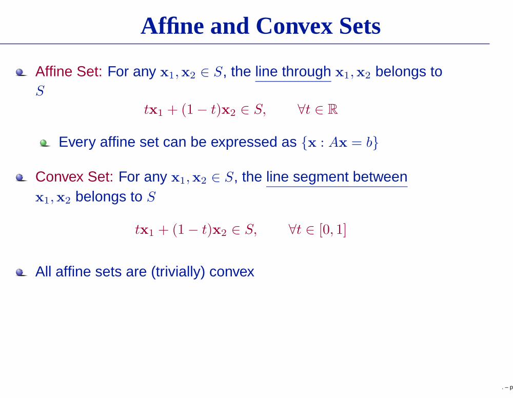
Affine and Convex Sets
Affine Set: For any x1,x2 ∈ S, the line through x1,x2 belongs toS
tx1 + (1 − t)x2 ∈ S, ∀t ∈ R
Every affine set can be expressed as {x : Ax = b}
Convex Set: For any x1,x2 ∈ S, the line segment betweenx1,x2 belongs to S
tx1 + (1 − t)x2 ∈ S, ∀t ∈ [0, 1]
All affine sets are (trivially) convex
. – p.2
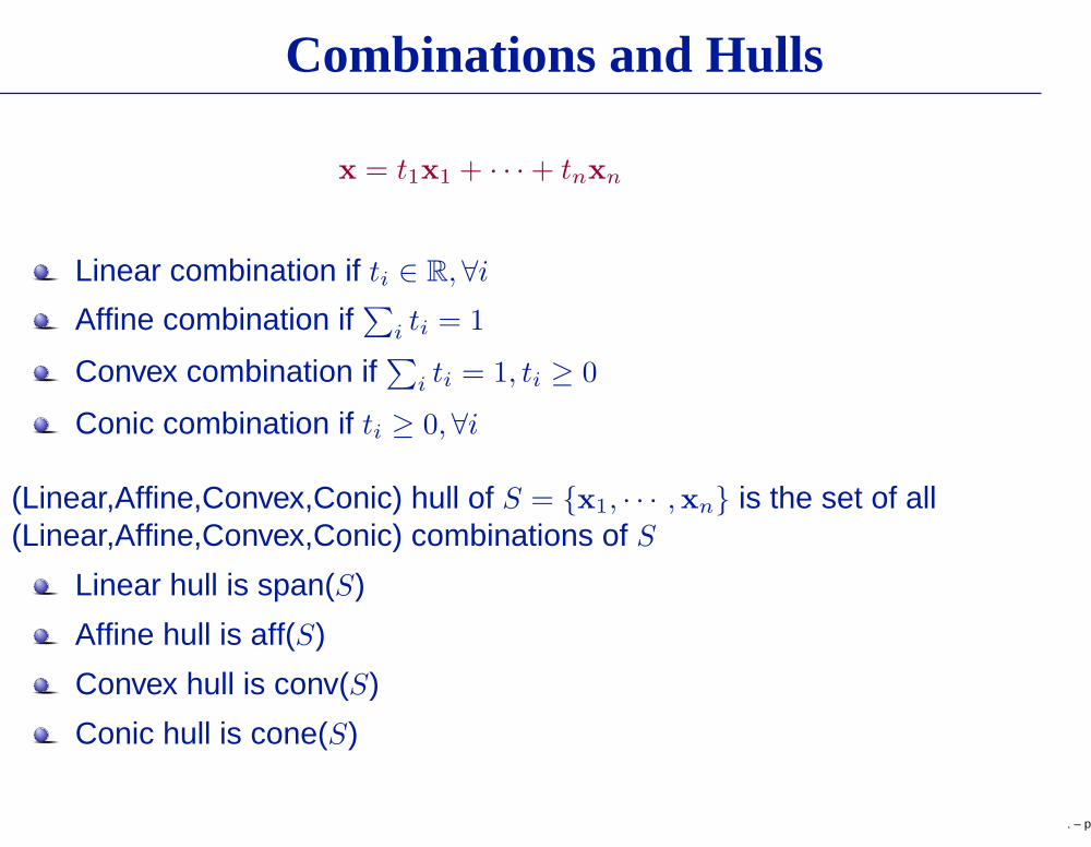
Combinations and Hulls
x = t1x1 + · · · + tnxn
Linear combination if ti ∈ R,∀i
Affine combination if∑
i ti = 1
Convex combination if∑
i ti = 1, ti ≥ 0
Conic combination if ti ≥ 0,∀i
(Linear,Affine,Convex,Conic) hull of S = {x1, · · · ,xn} is the set of all(Linear,Affine,Convex,Conic) combinations of S
Linear hull is span(S)
Affine hull is aff(S)
Convex hull is conv(S)
Conic hull is cone(S)
. – p.3
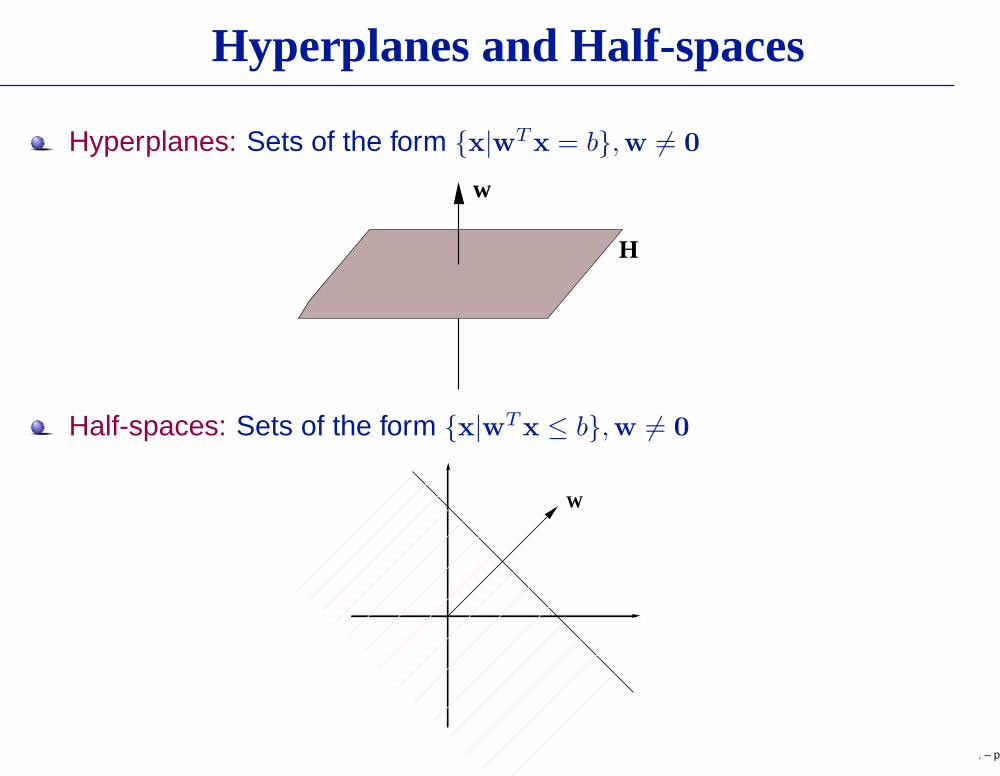
Hyperplanes and Half-spaces
Hyperplanes: Sets of the form {x|wTx = b},w 6= 0
w
H
Half-spaces: Sets of the form {x|wTx ≤ b},w 6= 0
� � � � � � � � � �
� � � � � � � � � �
� � � � � � � � � �
� � � � � � � � � �
� � � � � � � � � �
� � � � � � � � � �
� � � � � � � � � �
� � � � � � � � � �
� � � � � � � � � �
� � � � � � � � � �
� � � � � � � � �
� � � � � � � � �
� � � � � � � � �
� � � � � � � � �
� � � � � � � � �
� � � � � � � � �
� � � � � � � � �
� � � � � � � � �
� � � � � � � � �
� � � � � � � � �
� � � � � � � � �
� � � � � � � � �
� � � � � � � � �
� � � � � � � � �
� � � � � � � � �
� � � � � � � � �
� � � � � � � � �
� � � � � � � � �
� � � � � � � � �
� � � � � � � � �
� � � � � � � � �
� � � � � � � � �
� � � � � � � � �
� � � � � � � � �
� � � � � � � � �
� � � � � � � � �
� � � � � � � � �
� � � � � � � � �
� � � � � � � � �
� � � � � � � � �
� � � � � � � � �
� � � � � � � � �
� � � � � � � � �
� � � � � � � � �
� � � � � � � � �
� � � � � � � � �
� � � � � � � � �
� � � � � � � � �
� � � � � � � � �
� � � � � � � � �
� � � � � � � � �
� � � � � � � � �
� � � � � � � � �
� � � � � � � � �
� � � � � � � � �
� � � � � � � � �
� � � � � � � � �
� � � � � � � � �
� � � � � � � � �
� � � � � � � � �
� � � � � � � � �
� � � � � � � � �
� � � � � � � � �
� � � � � � � � �
� � � � � � � � �
� � � � � � � � �
� � � � � � � � �
� � � � � � � � �
� � � � � � � � �
� � � � � � � � �
� � � � � � � � �
� � � � � � � � �
� � � � � � � � �
� � � � � � � � �
� � � � � � � � �
� � � � � � � � �
� � � � � � � � �
� � � � � � � � �
� � � � � � � � �
� � � � � � � � �
� � � � � � � � �
� � � � � � � � �
� � � � � � � � �
� � � � � � � � �
� � � � � � � � �
� � � � � � � � �
� � � � � � � � �
� � � � � � � � �
� � � � � � � � �
� � � � � � � � �
� � � � � � � � �
� � � � � � � � �
� � � � � � � � �
� � � � � � � � �
� � � � � � � � �
� � � � � � � � �
� � � � � � � � �
� � � � � � � � �
� � � � � � � � �
� � � � � � � � �
� � � � � � � � �
� � � � � � � � �
� � � � � � � � �
� � � � � � � � �
� � � � � � � � �
� � � � � � � � �
� � � � � � � � �
� � � � � � � � �
� � � � � � � � �
� � � � � � � � �
� � � � � � � � �
� � � � � � � � �
� � � � � � � � �
� � � � � � � � �
� � � � � � � � �
� � � � � � � � �
� � � � � � � � �
� � � � � � � � �
� � � � � � � � �
� � � � � � � � �
� � � � � � � � �
� � � � � � � � �
� � � � � � � � �
� � � � � � � � �
� � � � � � � � � �
� � � � � � � � � �
� � � � � � � � � �
� � � � � � � � � �
� � � � � � � � � �
� � � � � � � � � �
� � � � � � � � � �
� � � � � � � � � �
� � � � � � � � � �
� � � � � � � � �
� � � � � � � � �
� � � � � � � � �
� � � � � � � � �
� � � � � � � � �
� � � � � � � � �
� � � � � � � � �
� � � � � � � � �
� � � � � � � � �
� � � � � � � � � �
� � � � � � � � � �
� � � � � � � � � �
� � � � � � � � � �
� � � � � � � � � �
� � � � � � � � � �
� � � � � � � � � �
� � � � � � � � � �
� � � � � � � � � �
� � � � � � � � � �
� � � � � � � � � �
� � � � � � � � � �
� � � � � � � � � �
� � � � � � � � � �
� � � � � � � � � �
� � � � � � � � � �
� � � � � � � � � �
� � � � � � � � � �
� � � � � � � � � �
� � � � � � � � � �
� � � � � � � � � �
� � � � � � � � � �
� � � � � � � � � �
� � � � � � � � � �
� � � � � � � � � �
� � � � � � � � � �
� � � � � � � � � �
� � � � � � � � �
� � � � � � � � �
� � � � � � � � �
� � � � � � � � �
� � � � � � � � �
� � � � � � � � �
� � � � � � � � �
� � � � � � � � �
� � � � � � � � �
� � � � � � � � � �
� � � � � � � � � �
� � � � � � � � � �
� � � � � � � � � �
� � � � � � � � � �
� � � � � � � � � �
� � � � � � � � � �
� � � � � � � � � �
� � � � � � � � � �
� � � � � � � � � �
� � � � � � � � �
� � � � � � � � �
� � � � � � � � �
� � � � � � � � �
� � � � � � � � �
� � � � � � � � �
� � � � � � � � �
� � � � � � � � �
� � � � � � � � �
� � � � � � � � � �
� � � � � � � � � �
� � � � � � � � � �
� � � � � � � � � �
� � � � � � � � � �
� � � � � � � � � �
� � � � � � � � � �
� � � � � � � � � �
� � � � � � � � � �
� � � � � � � � � �
� � � � � � � � � �
� � � � � � � � � �
� � � � � � � � � �
� � � � � � � � � �
� � � � � � � � � �
� � � � � � � � � �
� � � � � � � � � �
� � � � � � � � � �
� � � � � � � � � �
� � � � � � � � � �
� � � � � � � � � �
� � � � � � � � � �
� � � � � � � � � �
� � � � � � � � � �
� � � � � � � � � �
� � � � � � � � � �
� � � � � � � � � �
� � � � � � � � � �
� � � � � � � � � �
� � � � � � � � � �
� � � � � � � � � �
� � � � � � � � � �
� � � � � � � � � �
� � � � � � � � � �
� � � � � � � � � �
� � � � � � � � � �
� � � � � � � � � �
� � � � � � � � � �
� � � � � � � � � �
� � � � � � � � � �
W
. – p.4
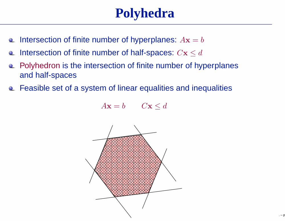
Polyhedra
Intersection of finite number of hyperplanes: Ax = b
Intersection of finite number of half-spaces: Cx ≤ d
Polyhedron is the intersection of finite number of hyperplanesand half-spaces
Feasible set of a system of linear equalities and inequalities
Ax = b Cx ≤ d
� � � � � � � � � � � � � �
� � � � � � � � � � � � � �
� � � � � � � � � � � � � �
� � � � � � � � � � � � � �
� � � � � � � � � � � � � �
� � � � � � � � � � � � � �
� � � � � � � � � � � � � �
� � � � � � � � � � � � � �
� � � � � � � � � � � � � �
� � � � � � � � � � � � � �
� � � � � � � � � � � � � �
� � � � � � � � � � � � � �
� � � � � � � � � � � � � �
� � � � � � � � � � � � � �
� � � � � � � � � � � � � �
� � � � � � � � � � � � � �
� � � � � � � � � � � � � �
� � � � � � � � � � � � � �
� � � � � � � � � � � � � �
� � � � � � � � � � � � � �
� � � � � � � � � � � � � �
� � � � � � � � � � � � � �
� � � � � � � � � � � � � �
� � � � � � � � � � � � � �
� � � � � � � � � � � � � �
� � � � � � � � � � � � � �
� � � � � � � �
� � � � � � � �
� � � � � � � �
� � � � � � � �
� � � � � � � �
� � � � � � � �
� � � � � � � �
� � � � � � � �
� � � � � � � �
� � � � � � � �
� � � � � � � �
� � � � � � � �
� � � � � � � �
� � � � � � � �
� � � � � � � �
� � � � � � � �
� � � � � � � �
� � � � � � � �
� � � � � � � �
� � � � � � � �
� � � � � � � �
� � � � � � � �
! ! ! ! !
! ! ! ! !
! ! ! ! !
! ! ! ! !
! ! ! ! !
! ! ! ! !
! ! ! ! !
! ! ! ! !
! ! ! ! !
! ! ! ! !
! ! ! ! !
! ! ! ! !
" " " " " " " " " " " " " " " "
" " " " " " " " " " " " " " " "
" " " " " " " " " " " " " " " "
# # # # # # # # # # # # # # # #
# # # # # # # # # # # # # # # #
# # # # # # # # # # # # # # # #
$ $ $ $ $ $ $ $ $ $
$ $ $ $ $ $ $ $ $ $
$ $ $ $ $ $ $ $ $ $
$ $ $ $ $ $ $ $ $ $
$ $ $ $ $ $ $ $ $ $
$ $ $ $ $ $ $ $ $ $
$ $ $ $ $ $ $ $ $ $
$ $ $ $ $ $ $ $ $ $
$ $ $ $ $ $ $ $ $ $
$ $ $ $ $ $ $ $ $ $
$ $ $ $ $ $ $ $ $ $
$ $ $ $ $ $ $ $ $ $
% % % % % % % % % %
% % % % % % % % % %
% % % % % % % % % %
% % % % % % % % % %
% % % % % % % % % %
% % % % % % % % % %
% % % % % % % % % %
% % % % % % % % % %
% % % % % % % % % %
% % % % % % % % % %
% % % % % % % % % %
% % % % % % % % % %
& & & & &
& & & & &
& & & & &
& & & & &
& & & & &
& & & & &
& & & & &
& & & & &
& & & & &
& & & & &
& & & & &
' ' ' ' '
' ' ' ' '
' ' ' ' '
' ' ' ' '
' ' ' ' '
' ' ' ' '
' ' ' ' '
' ' ' ' '
' ' ' ' '
' ' ' ' '
' ' ' ' '
( ( ( ( ( ( ( ( ( ( ( ( (
( ( ( ( ( ( ( ( ( ( ( ( (
) ) ) ) ) ) ) ) ) ) ) ) )
) ) ) ) ) ) ) ) ) ) ) ) )
. – p.5

Convex Sets, Reloaded
A polyhedron is a convex set
. – p.6

Convex Sets, Reloaded
A polyhedron is a convex set
Intersection of half-spaces is always a convex set
. – p.6
Convex Sets, Reloaded
A polyhedron is a convex set
Intersection of half-spaces is always a convex set
Any convex set can be expressed as an intersection of (possiblyinfinite) half-spaces
Think of a square, circle, ellipse
. – p.6

Convex Sets, Reloaded
A polyhedron is a convex set
Intersection of half-spaces is always a convex set
Any convex set can be expressed as an intersection of (possiblyinfinite) half-spaces
Think of a square, circle, ellipse
Two equivalent but different points of viewS is convex, if ∀x1,x2 ∈ S, tx1 + (1 − t)x2 ∈ S, ∀t ∈ [0, 1]
S is convex, if it is the intersection of all half-spacescontaining it
This is the key reason behind (Legendre) Duality
. – p.6

Convex Functions
A function f is convex if dom(f ) is a convex set and ∀t ∈ [0, 1]
f(tx1 + (1 − t)x2) ≤ tf(x1) + (1 − t)f(x2)
A function f is concave if −f is convex
. – p.7
Examples
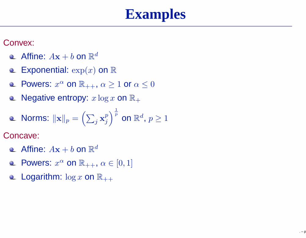
Convex:
Affine: Ax + b on Rd
Exponential: exp(x) on R
Powers: xα on R++, α ≥ 1 or α ≤ 0
Negative entropy: x log x on R+
Norms: ‖x‖p =(
∑
j xpj
)1
p
on Rd, p ≥ 1
Concave:
Affine: Ax + b on Rd
Powers: xα on R++, α ∈ [0, 1]
Logarithm: log x on R++
. – p.8

Epigraph
Epigraph of a function f(x), epi(f ), is the setS = {(x, v) ∈ R
d+1|v ≥ f(x)}
Everything that lies on or above the function
. – p.9

Epigraph
Epigraph of a function f(x), epi(f ), is the setS = {(x, v) ∈ R
d+1|v ≥ f(x)}
Everything that lies on or above the function
If f is a convex function, epi(f ) is a convex set in Rd+1
. – p.9

Epigraph
Epigraph of a function f(x), epi(f ), is the setS = {(x, v) ∈ R
d+1|v ≥ f(x)}
Everything that lies on or above the function
If f is a convex function, epi(f ) is a convex set in Rd+1
A function f is convex if and only if epi(f ) is a convex setRecall: A set is convex if it is an intersection of half-spaces
Half-spaces in Rd+1 are epigraphs of affine functions in R
d
A convex function f is the pointwise supremum of allaffine functions majorized by f
. – p.9

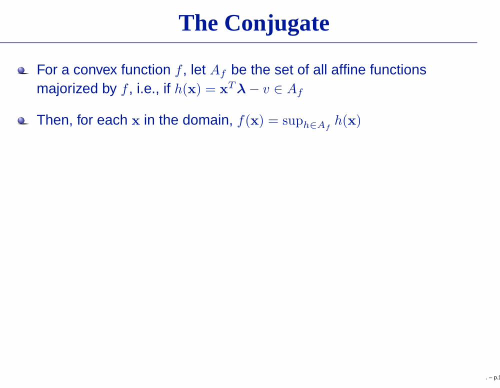
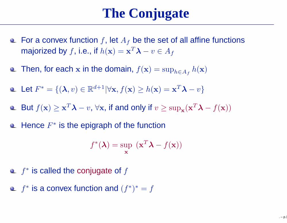
The Conjugate
For a convex function f , let Af be the set of all affine functionsmajorized by f , i.e., if h(x) = x
Tλ − v ∈ Af
. – p.10
The Conjugate
For a convex function f , let Af be the set of all affine functionsmajorized by f , i.e., if h(x) = x
Tλ − v ∈ Af
Then, for each x in the domain, f(x) = suph∈Afh(x)
. – p.10

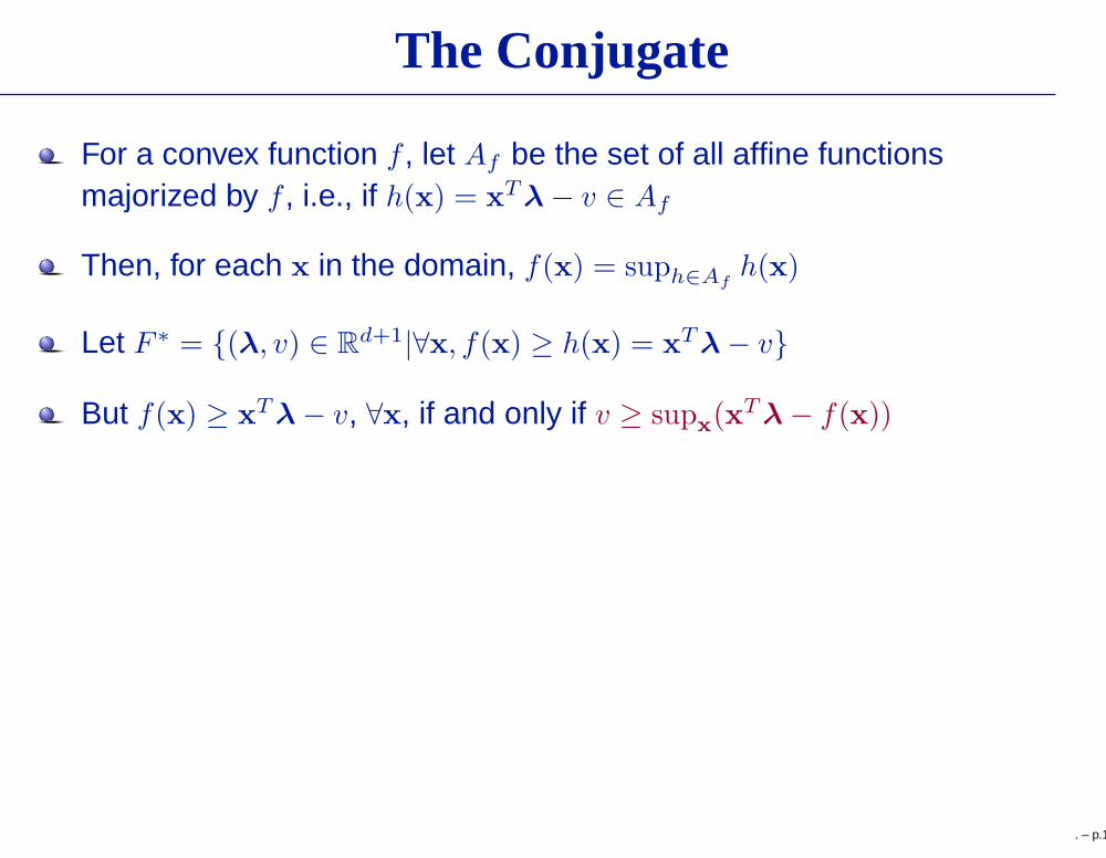
The Conjugate
For a convex function f , let Af be the set of all affine functionsmajorized by f , i.e., if h(x) = x
Tλ − v ∈ Af
Then, for each x in the domain, f(x) = suph∈Afh(x)
Let F ∗ = {(λ, v) ∈ Rd+1|∀x, f(x) ≥ h(x) = x
Tλ − v}
. – p.10
The Conjugate
For a convex function f , let Af be the set of all affine functionsmajorized by f , i.e., if h(x) = x
Tλ − v ∈ Af
Then, for each x in the domain, f(x) = suph∈Afh(x)
Let F ∗ = {(λ, v) ∈ Rd+1|∀x, f(x) ≥ h(x) = x
Tλ − v}
But f(x) ≥ xTλ − v, ∀x, if and only if v ≥ sup
x(xT
λ − f(x))
. – p.10

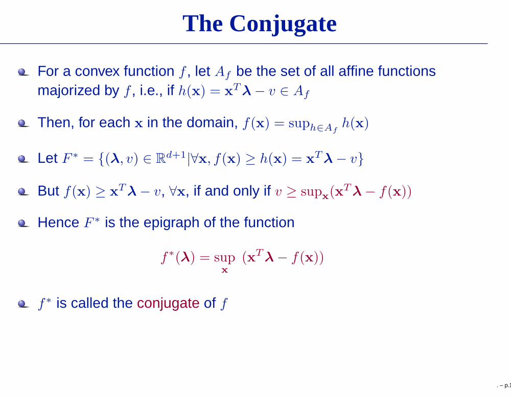
The Conjugate
For a convex function f , let Af be the set of all affine functionsmajorized by f , i.e., if h(x) = x
Tλ − v ∈ Af
Then, for each x in the domain, f(x) = suph∈Afh(x)
Let F ∗ = {(λ, v) ∈ Rd+1|∀x, f(x) ≥ h(x) = x
Tλ − v}
But f(x) ≥ xTλ − v, ∀x, if and only if v ≥ sup
x(xT
λ − f(x))
Hence F ∗ is the epigraph of the function
f∗(λ) = supx
(xTλ − f(x))
. – p.10
The Conjugate
For a convex function f , let Af be the set of all affine functionsmajorized by f , i.e., if h(x) = x
Tλ − v ∈ Af
Then, for each x in the domain, f(x) = suph∈Afh(x)
Let F ∗ = {(λ, v) ∈ Rd+1|∀x, f(x) ≥ h(x) = x
Tλ − v}
But f(x) ≥ xTλ − v, ∀x, if and only if v ≥ sup
x(xT
λ − f(x))
Hence F ∗ is the epigraph of the function
f∗(λ) = supx
(xTλ − f(x))
f∗ is called the conjugate of f
f∗ is a convex function and (f∗)∗ = f
. – p.10
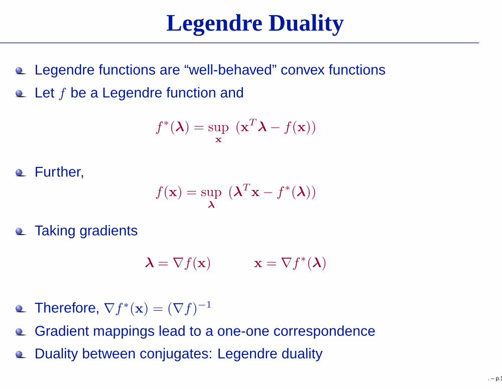
Legendre Duality
Legendre functions are “well-behaved” convex functions
Let f be a Legendre function and
f∗(λ) = supx
(xTλ − f(x))
Further,f(x) = sup
λ
(λTx − f∗(λ))
Taking gradients
λ = ∇f(x) x = ∇f∗(λ)
Therefore, ∇f∗(x) = (∇f)−1
Gradient mappings lead to a one-one correspondence
Duality between conjugates: Legendre duality
. – p.11

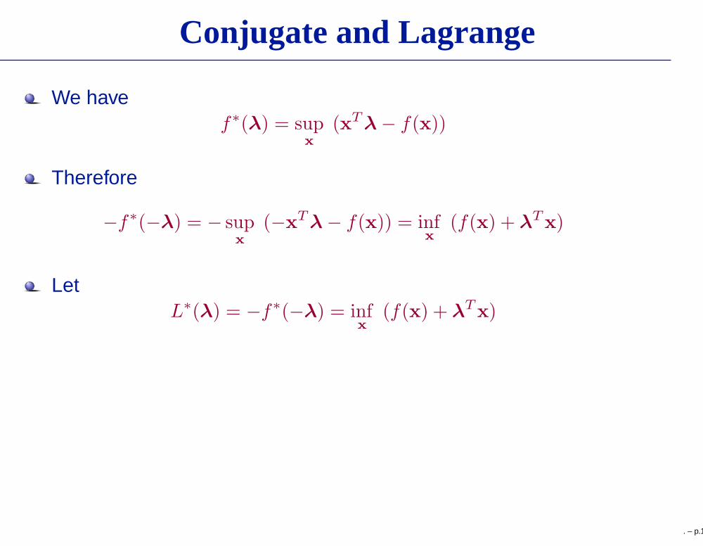
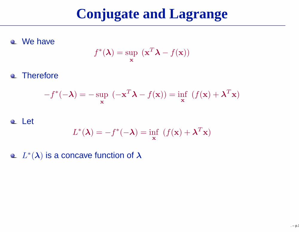
Conjugate and Lagrange
We havef∗(λ) = sup
x
(xTλ − f(x))
. – p.12

Conjugate and Lagrange
We havef∗(λ) = sup
x
(xTλ − f(x))
Therefore
−f∗(−λ) = − supx
(−xTλ − f(x)) = inf
x
(f(x) + λTx)
. – p.12
Conjugate and Lagrange
We havef∗(λ) = sup
x
(xTλ − f(x))
Therefore
−f∗(−λ) = − supx
(−xTλ − f(x)) = inf
x
(f(x) + λTx)
LetL∗(λ) = −f∗(−λ) = inf
x
(f(x) + λTx)
. – p.12
Conjugate and Lagrange
We havef∗(λ) = sup
x
(xTλ − f(x))
Therefore
−f∗(−λ) = − supx
(−xTλ − f(x)) = inf
x
(f(x) + λTx)
LetL∗(λ) = −f∗(−λ) = inf
x
(f(x) + λTx)
L∗(λ) is a concave function of λ
. – p.12

Conjugate and Lagrange
We havef∗(λ) = sup
x
(xTλ − f(x))
Therefore
−f∗(−λ) = − supx
(−xTλ − f(x)) = inf
x
(f(x) + λTx)
LetL∗(λ) = −f∗(−λ) = inf
x
(f(x) + λTx)
L∗(λ) is a concave function of λ
L∗(λ) will turn out to be the Lagrange dual
. – p.12

Constrained Optimization
The equality & inequality constrained optimization problem
minimize f(x)
subject to hi(x) = 0 i = 1, . . . , m
gj(x) ≤ 0 j = 1, . . . , n
. – p.13

Constrained Optimization
The equality & inequality constrained optimization problem
minimize f(x)
subject to hi(x) = 0 i = 1, . . . , m
gj(x) ≤ 0 j = 1, . . . , n
The Lagrangian
L(x, λ, ν) = f(x) + λT h(x) + ν
T g(x)
= f(x) +
m∑
i=1
λihi(x) +
n∑
j=1
νjgj(x)
. – p.13
Constrained Optimization
The equality & inequality constrained optimization problem
minimize f(x)
subject to hi(x) = 0 i = 1, . . . , m
gj(x) ≤ 0 j = 1, . . . , n
The Lagrangian
L(x, λ, ν) = f(x) + λT h(x) + ν
T g(x)
= f(x) +
m∑
i=1
λihi(x) +
n∑
j=1
νjgj(x)
{λi}mi=1, {νj}
nj=1 are the Lagrange multipliers
. – p.13
Lagrange Dual
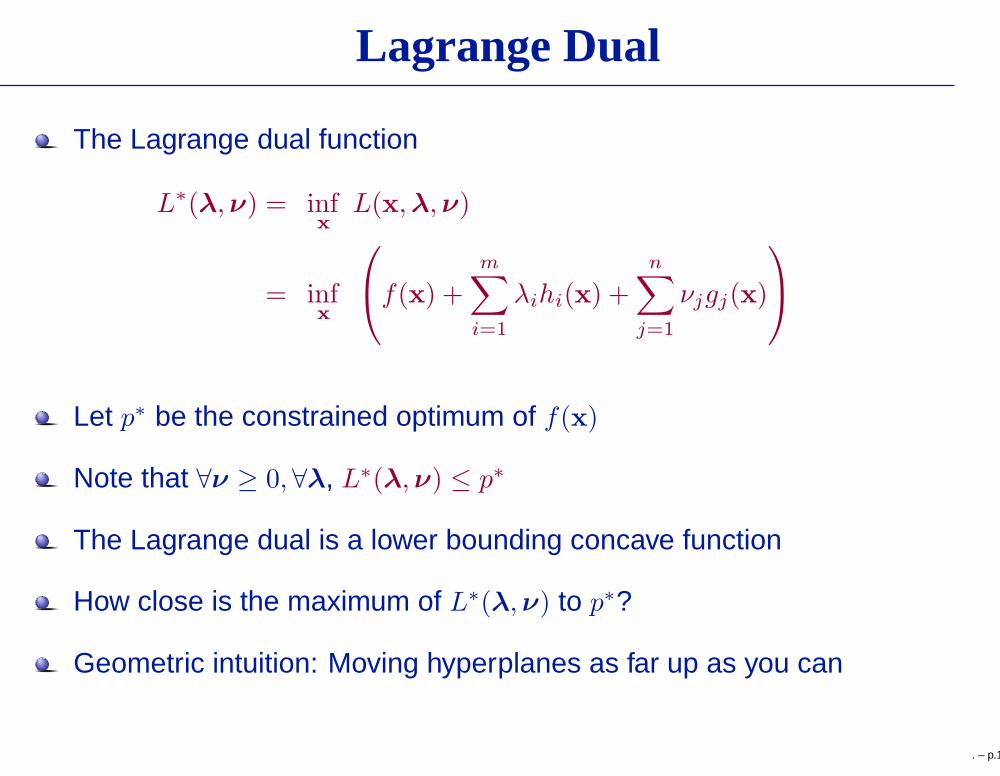
The Lagrange dual function
L∗(λ, ν) = infx
L(x, λ, ν)
= infx
f(x) +
m∑
i=1
λihi(x) +
n∑
j=1
νjgj(x)
. – p.14
Lagrange Dual
The Lagrange dual function
L∗(λ, ν) = infx
L(x, λ, ν)
= infx
f(x) +
m∑
i=1
λihi(x) +
n∑
j=1
νjgj(x)
Let p∗ be the constrained optimum of f(x)
. – p.14

Lagrange Dual
The Lagrange dual function
L∗(λ, ν) = infx
L(x, λ, ν)
= infx
f(x) +
m∑
i=1
λihi(x) +
n∑
j=1
νjgj(x)
Let p∗ be the constrained optimum of f(x)
Note that ∀ν ≥ 0,∀λ, L∗(λ, ν) ≤ p∗
. – p.14
Lagrange Dual
The Lagrange dual function
L∗(λ, ν) = infx
L(x, λ, ν)
= infx
f(x) +
m∑
i=1
λihi(x) +
n∑
j=1
νjgj(x)
Let p∗ be the constrained optimum of f(x)
Note that ∀ν ≥ 0,∀λ, L∗(λ, ν) ≤ p∗
The Lagrange dual is a lower bounding concave function
. – p.14

Lagrange Dual
The Lagrange dual function
L∗(λ, ν) = infx
L(x, λ, ν)
= infx
f(x) +
m∑
i=1
λihi(x) +
n∑
j=1
νjgj(x)
Let p∗ be the constrained optimum of f(x)
Note that ∀ν ≥ 0,∀λ, L∗(λ, ν) ≤ p∗
The Lagrange dual is a lower bounding concave function
How close is the maximum of L∗(λ, ν) to p∗?
. – p.14
Lagrange Dual
The Lagrange dual function
L∗(λ, ν) = infx
L(x, λ, ν)
= infx
f(x) +
m∑
i=1
λihi(x) +
n∑
j=1
νjgj(x)
Let p∗ be the constrained optimum of f(x)
Note that ∀ν ≥ 0,∀λ, L∗(λ, ν) ≤ p∗
The Lagrange dual is a lower bounding concave function
How close is the maximum of L∗(λ, ν) to p∗?
Geometric intuition: Moving hyperplanes as far up as you can
. – p.14

An Example
minimize xTx
subject to Ax = b
Lagrangian L(x, λ) = xTx + λ
T (Ax − b)
Recall that L∗(λ) = infx L(x, λ)
Setting gradient to 0, x = − 1
2AT
λ
Hence, the dual
L∗(λ) = L
(
−1
2AT
λ, λ
)
= −1
4λ
T AATλ − λ
T b
L∗(λ) is a lower bounding concave function
. – p.15
Lagrange Duality and The Conjugate
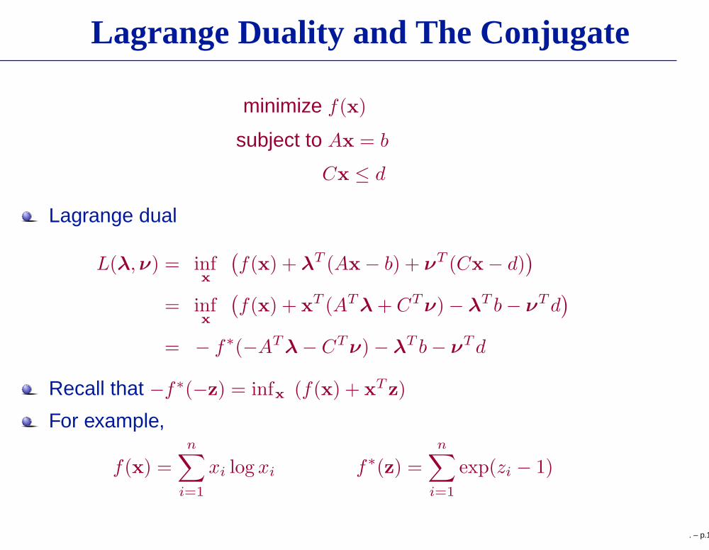
minimize f(x)
subject to Ax = b
Cx ≤ d
Lagrange dual
L(λ, ν) = infx
(
f(x) + λT (Ax − b) + ν
T (Cx − d))
= infx
(
f(x) + xT (AT
λ + CTν) − λ
T b − νT d
)
= − f∗(−ATλ − CT
ν) − λT b − ν
T d
Recall that −f∗(−z) = infx (f(x) + xTz)
For example,
f(x) =
n∑
i=1
xi log xi f∗(z) =
n∑
i=1
exp(zi − 1)
. – p.16
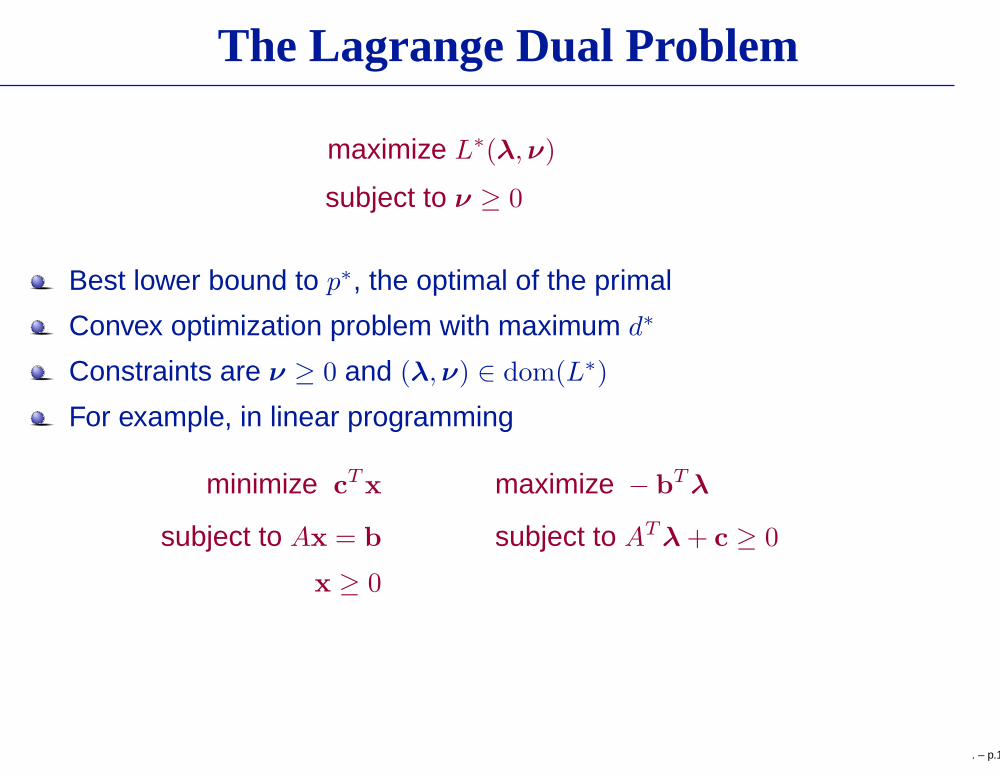
The Lagrange Dual Problem
maximize L∗(λ, ν)
subject to ν ≥ 0
Best lower bound to p∗, the optimal of the primal
Convex optimization problem with maximum d∗
Constraints are ν ≥ 0 and (λ, ν) ∈ dom(L∗)
For example, in linear programming
minimize cTx maximize − b
Tλ
subject to Ax = b subject to ATλ + c ≥ 0
x ≥ 0
. – p.17

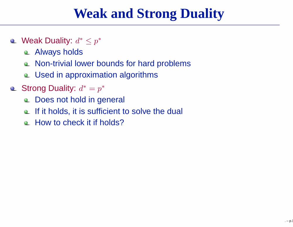
Weak and Strong Duality
Weak Duality: d∗ ≤ p∗
Always holdsNon-trivial lower bounds for hard problemsUsed in approximation algorithms
. – p.18
Weak and Strong Duality
Weak Duality: d∗ ≤ p∗
Always holdsNon-trivial lower bounds for hard problemsUsed in approximation algorithms
Strong Duality: d∗ = p∗
Does not hold in generalIf it holds, it is sufficient to solve the dualHow to check it if holds?
. – p.18

Weak and Strong Duality
Weak Duality: d∗ ≤ p∗
Always holdsNon-trivial lower bounds for hard problemsUsed in approximation algorithms
Strong Duality: d∗ = p∗
Does not hold in generalIf it holds, it is sufficient to solve the dualHow to check it if holds?
Constraint QualificationNormally true on convex problemsTrue if the convex problem is strictly feasibleSlater’s Condition for strong dualityThere are other ways to check strong duality
. – p.18

Example: Quadratic Programs
minimize xTx
subject to Ax ≤ b
Lagrange dual
L∗(ν) = infx
(
xTx + ν
T (Ax − b))
= −1
4ν
T AATν − bT
ν
Dual problem
maximize −1
4ν
T AATν − bT
ν
subject to ν ≥ 0
From Slater’s condition, p∗ = d∗
It is sufficient to solve the dual
. – p.19
Complementary Slackness
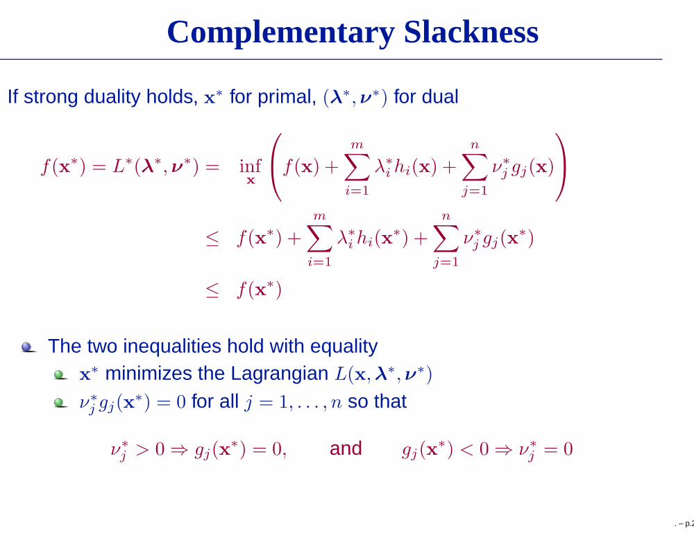
If strong duality holds, x∗ for primal, (λ∗, ν∗) for dual
f(x∗) = L∗(λ∗, ν∗) = infx
f(x) +
m∑
i=1
λ∗
i hi(x) +
n∑
j=1
ν∗
j gj(x)
≤ f(x∗) +
m∑
i=1
λ∗
i hi(x∗) +
n∑
j=1
ν∗
j gj(x∗)
≤ f(x∗)
The two inequalities hold with equalityx∗ minimizes the Lagrangian L(x, λ∗, ν∗)
ν∗
j gj(x∗) = 0 for all j = 1, . . . , n so that
ν∗
j > 0 ⇒ gj(x∗) = 0, and gj(x
∗) < 0 ⇒ ν∗
j = 0
. – p.20

Karush-Kuhn-Tucker (KKT) Conditions
Necessary conditions satisfied by any primal and dual optimal pairsx̃ and (λ̃, ν̃)
Primal Feasibility:
hi(x̃) = 0, i = 1, . . . , n, gj(x̃) ≤ 0, j = 1, . . . , m
Dual Feasibility:ν̃j ≥ 0, j = 1, . . . , m
Complementary Slackness:
ν̃jgj(x̃) = 0, j = 1, . . . , m
Gradient condition:
∇f(x̃) +
n∑
i=1
λ̃i∇hi(x̃) +
m∑
j=1
ν̃j∇gj(x̃) = 0
The conditions are sufficient for a convex problem. – p.21


![RobustSampled –Data ControlofSwitched Affine Systemsemilia/TAC13.pdf · switched affine systems with a sampled-data switching law. ... on optimal control methods [12], ... Note](https://img.pdfslide.us/doc/110x75/5b8aed2e7f8b9a82418d16b9/robustsampled-data-controlofswitched-afne-emiliatac13pdf-switched-afne.jpg)