Converting Analog Controllers to Smart Controllers with ... · SPRA995 4 Converting Analog Controllers to Smart Controllers with the TMS320C2000 DSPs • Ease of implementation: Functions

Application ReportSPRA995 − June 2004

1

Converting Analog Controllers to Smart Controllers withthe TMS320C2000 DSPs

Kedar Godbole DSP Digital Control Systems

ABSTRACT

Modern applications demand faster, cheaper, and better motor control systems, and theperformance demanded from embedded motor controllers is ever increasing. Programmablecontrollers offer the unique opportunity to improve performance, reduce cost, and enabledesigners to improve the efficiency of motor control systems. Such performance objectivestypically need advanced algorithms that are computationally intensive and are bestimplemented on digital signal processors (DSPs).

For most engineers looking to implement control algorithms on DSPs, they are faced with asignificant barrier – a definite lack of comprehensive information on the process of achievingthe conversion.

Texas Instruments (TI) has constructed a comprehensive portfolio of control solutions withthe TMS320C2000 DSP controllers, to assist with this conversion process. This applicationnote provides an overview of the process used to convert an existing legacy analog ormicrocontroller-based solution into a DSP-enabled solution.

Contents

1 Motivation 3. . . . . . . . . . . . . . . . . . . . . . . . . . . . . . . . . . . . . . . . . . . . . . . . . . . . . . . . . . . . . . . . . . . . . . . . . . .

2 Analog Controllers vs Digital Controllers 3. . . . . . . . . . . . . . . . . . . . . . . . . . . . . . . . . . . . . . . . . . . . . . 2.1 Comparative Strengths of Digital Controllers 3. . . . . . . . . . . . . . . . . . . . . . . . . . . . . . . . . . . . . . . . . 2.2 Digital Controller Issues Needing Management 4. . . . . . . . . . . . . . . . . . . . . . . . . . . . . . . . . . . . . . .

3 Converting Analog Controllers to DSP based Digital Controllers 5. . . . . . . . . . . . . . . . . . . . . . . . 3.1 System Identification 5. . . . . . . . . . . . . . . . . . . . . . . . . . . . . . . . . . . . . . . . . . . . . . . . . . . . . . . . . . . . . .

3.1.1 System Identification for the Example System in Figure 2 7. . . . . . . . . . . . . . . . . . . . . . . 3.1.2 Controller Selection 8. . . . . . . . . . . . . . . . . . . . . . . . . . . . . . . . . . . . . . . . . . . . . . . . . . . . . . . . 3.1.3 What Goes Inside that Box Marked “Controller”? 9. . . . . . . . . . . . . . . . . . . . . . . . . . . . . . .

3.2 System Analysis 10. . . . . . . . . . . . . . . . . . . . . . . . . . . . . . . . . . . . . . . . . . . . . . . . . . . . . . . . . . . . . . . . . 3.2.1 Create a Block Diagram 10. . . . . . . . . . . . . . . . . . . . . . . . . . . . . . . . . . . . . . . . . . . . . . . . . . . . 3.2.2 Identify Controllers Which are to be Converted into Digital Controllers 11. . . . . . . . . . . .

3.3 Create a Mathematical Definition for the System 11. . . . . . . . . . . . . . . . . . . . . . . . . . . . . . . . . . . . . 3.3.1 The Controller Gain 11. . . . . . . . . . . . . . . . . . . . . . . . . . . . . . . . . . . . . . . . . . . . . . . . . . . . . . . 3.3.2 The Output Amplifier 11. . . . . . . . . . . . . . . . . . . . . . . . . . . . . . . . . . . . . . . . . . . . . . . . . . . . . . 3.3.3 Plant Transfer Function 11. . . . . . . . . . . . . . . . . . . . . . . . . . . . . . . . . . . . . . . . . . . . . . . . . . . . 3.3.4 Sensor Gain 12. . . . . . . . . . . . . . . . . . . . . . . . . . . . . . . . . . . . . . . . . . . . . . . . . . . . . . . . . . . . . . 3.3.5 Loop Gain 12. . . . . . . . . . . . . . . . . . . . . . . . . . . . . . . . . . . . . . . . . . . . . . . . . . . . . . . . . . . . . . . .

Trademarks are the property of their respective owners.

SPRA995

2 Converting Analog Controllers to Smart Controllers with the TMS320C2000 DSPs

3.4 Partition the System into “Hardware Components” and “Software Components” 12. . . . . . . . . 3.5 Quantization of Signals, Analog Range and Scaling 17. . . . . . . . . . . . . . . . . . . . . . . . . . . . . . . . . . 3.6 Anti-Aliasing Considerations 19. . . . . . . . . . . . . . . . . . . . . . . . . . . . . . . . . . . . . . . . . . . . . . . . . . . . . . 3.7 Design Discrete Time Controllers to Implement the Control Function 20. . . . . . . . . . . . . . . . . . . 3.8 Choosing Sampling Rates in a Quantized Discrete Time Domain System 21. . . . . . . . . . . . . . .

4 Implementing Fixed-Point Arithmetic: F2812 and IQ Math Make it Easy 23. . . . . . . . . . . . . . . . .

5 Leveraging Existing Collateral: Reduce Time to Market 24. . . . . . . . . . . . . . . . . . . . . . . . . . . . . . . .

6 Conclusion 24. . . . . . . . . . . . . . . . . . . . . . . . . . . . . . . . . . . . . . . . . . . . . . . . . . . . . . . . . . . . . . . . . . . . . . . . .

7 References 25. . . . . . . . . . . . . . . . . . . . . . . . . . . . . . . . . . . . . . . . . . . . . . . . . . . . . . . . . . . . . . . . . . . . . . . . .

List of Figures

Figure 1 Flowchart for Converting an Analog Control System to aDigital Controller Implementation 6. . . . . . . . . . . . . . . . . . . . . . . . . . . . . . . . . . . . . . . . . . . . . . . .

Figure 2 A Sample Control System 7. . . . . . . . . . . . . . . . . . . . . . . . . . . . . . . . . . . . . . . . . . . . . . . . . . . . . . Figure 3 System Identification for Example System in Figure 2 8. . . . . . . . . . . . . . . . . . . . . . . . . . . . . . Figure 4 The Controller 8. . . . . . . . . . . . . . . . . . . . . . . . . . . . . . . . . . . . . . . . . . . . . . . . . . . . . . . . . . . . . . . . Figure 5 Error Based Control 9. . . . . . . . . . . . . . . . . . . . . . . . . . . . . . . . . . . . . . . . . . . . . . . . . . . . . . . . . . . Figure 6 Proportional Controller 9. . . . . . . . . . . . . . . . . . . . . . . . . . . . . . . . . . . . . . . . . . . . . . . . . . . . . . . . . Figure 7 Proportional-Integral Controller 9. . . . . . . . . . . . . . . . . . . . . . . . . . . . . . . . . . . . . . . . . . . . . . . . . Figure 8 Proportional-Integral-Derivative Controller 10. . . . . . . . . . . . . . . . . . . . . . . . . . . . . . . . . . . . . . . Figure 9 Block Diagram for Sample System in Figure 3 10. . . . . . . . . . . . . . . . . . . . . . . . . . . . . . . . . . . Figure 10 Block Diagram for a TMS320F2812 DSP controller 13. . . . . . . . . . . . . . . . . . . . . . . . . . . . . . . Figure 11 Digital and Analog Portions of a Control System 14. . . . . . . . . . . . . . . . . . . . . . . . . . . . . . . . . Figure 12 A Digital Implementation for the Sample System in Figure 2 15. . . . . . . . . . . . . . . . . . . . . . . Figure 13 System Partitioning for Field-Oriented Control of a

Permanent Magnet Synchronous Motor 16. . . . . . . . . . . . . . . . . . . . . . . . . . . . . . . . . . . . . . . . . Figure 14 Software Block Diagram for the PMSM Field-Oriented Control 17. . . . . . . . . . . . . . . . . . . . . Figure 15 Quantization of Analog Signals During A-to-D Conversion With a

Hypothetical 4-Bit Converter 18. . . . . . . . . . . . . . . . . . . . . . . . . . . . . . . . . . . . . . . . . . . . . . . . . . . Figure 16 Frequency Remapping With Conversion to a Sampled Discrete Time System 19. . . . . . . . Figure 17 How Aliasing Generates a Fictitious Low-Frequency Signal 20. . . . . . . . . . . . . . . . . . . . . . . . Figure 18 Converting Code from Floating Point to IQMath 23. . . . . . . . . . . . . . . . . . . . . . . . . . . . . . . . . .

List of Tables

Table 1 Discrete Time Controller Coefficients 22. . . . . . . . . . . . . . . . . . . . . . . . . . . . . . . . . . . . . . . . . . . Table 2 TI Foundation Software 24. . . . . . . . . . . . . . . . . . . . . . . . . . . . . . . . . . . . . . . . . . . . . . . . . . . . . . .

SPRA995


1 MotivationModern high-performance motor controllers are expected to concurrently achieve severalobjectives. They must meet or exceed the dynamical specifications, and in addition, they mustsatisfy several other requirements. Examples are high efficiency, power factor, andelectromagnetic compatibility (EMC).

To meet all these requirements, designers are turning to mathematical algorithms that arecomputationally demanding.

Digital signal processors provide an excellent means to implement controllers to meet this goal,but one of the major barriers that designers are faced with is the lack of a clear process anddocumentation on how to bring everything together. There are several excellent applicationexamples, which describe specific applications. Several excellent textbooks discuss, in detail,the mathematics needed to model, design, and analyze discrete time-sampled data controllers.

However, all of these seem to either assume that the designer has either already implementedthe conversion from the analog control system to a digital one, and just needs to know how todesign the controllers, or has a specific application that is served exactly by a specificapplication example.

This application note aims to provide a bridge to help designers make the conversion; however,it does not intend to be adequate to describe in any detail the mathematics of discretecontrollers, for example. For that background, the reader should refer one of the severaltextbooks on the subject, included in the references section of this application note.

Texas Instruments has put together a comprehensive portfolio of solutions to help, and thisapplication note will point to several of those for typical examples.

2 Analog Controllers vs Digital ControllersIn order to convert analog controllers to digital controllers, the first step is to gain anunderstanding of the strengths and weaknesses of both forms of controllers.

2.1 Comparative Strengths of Digital Controllers

Digital controllers offer several advantages, which make a very convincing case forimplementing new controllers with digital techniques – and converting existing analog controllersto new, digital implementations.

Some of these advantages are:

• Programmability brings new opportunities to the table: Programmable DSP controllersoffer new capabilities, such as implementing advanced algorithms for motor control, whichenable higher performance, and lower energy consumption, among other things.

• Digital controllers are immune to drifts: Digital controllers work with elements thatoperate in saturation, well outside the linear operation. As such, their functioning issubstantially unaffected by either time or temperature drifts. Equations in software do notdrift, so the definitions of the control laws remain consistent, unlike analog controllers.

• Software can automate calibration: Even with digital controllers, there is a significantamount of analog circuitry wrapped around the controller. However, software implementedon programmable controllers can calibrate out the inaccuracies, and software can automatethis calibration process. This lowers the cost of manufacturing by eliminating a manualcalibration step.

SPRA995


• Ease of implementation: Functions are easily implemented in software. It is far easier tocode the equation ‘x=y+z;’ in software than it is to design an analog circuit to do the addition.

• Faster time to market: Programmable digital controllers make it possible to leverageexisting off-the-shelf controllers, which allow the fastest realization of a design. In addition,the design of controllers is often an iterative process, with repeated design and test steps,until the specifications are met. Such an iterative process can be executed very rapidly bymeans of a software-configurable controller. Such a controller can be configured in minutes,versus a circuit change, which is not easy.

Trimming gains can also be done on-line, which gives designers a friendly means ofchanging the control system while observing the system response.

• Control law changes are software updates: During system design, often it becomesnecessary to change the control law, beyond just changing the gains. A new structure maybe needed, or a boundary condition must be covered. Making changes to analog controllersis a very slow process. For programmable controllers, it is a matter of designing thecontroller, and then changing the coefficients in software. Flexibility during design is key tofaster system design.

• Far less sensitive to component tolerances: Digital controllers are far less susceptible tocomponent tolerances. Since they implement algorithms in software, gains and parametersare far more consistent and reproducible.

2.2 Digital Controller Issues Needing Management

Digital controllers require somewhat of a new approach, and there are considerations that mustbe taken into account when designing a system with a digital signal controller.

• Quantization affects controller implementation: Controllers implemented in both fixedand floating-point DSPs are affected by quantization. For fixed-point numbers, the number ofbits used to represent the number quite directly determines the precision of therepresentation. Designers must understand and manage how this precision affects theircontrol system.

Fortunately, new 32-bit DSP controllers such as the TMS320F2812 offer designers a 32-bitcomputation capability for control – this makes quantization all but disappear. At 32 bits,resolution is 1 part in 4,294,967,296 which corresponds to a precision of 0.0000000232% –this is usually adequate for most controllers.

Contrary to first appearances, floating-point processors do not necessarily offer betterprecision. Many 32-bit wide representations of floating-point numbers have 24 bits for themantissa, and this is far less resolution than a fixed point controller for the same number ofbits. Floating-point numbers excel in providing dynamic range, not resolution.

• Digital controllers mean designers must work with discrete time math: One of the mostimportant challenges in working with discretized controllers is that designers must work inthe z-plane, and get used to discrete time-design considerations. This is usually quite arewarding experience; most system designers are able to readjust to using z-transforms andconverting from s-plane to z-plane with ease.

SPRA995


3 Converting Analog Controllers to DSP based Digital Controllers

To convert an analog controller to a DSP-based digital control system involves understandingthe existing system, and then creating an equivalent system with a DSP-based controller, thathas the desired performance characteristics. Often this is a two-step process; first creating anequivalent, and then adding in additional features.

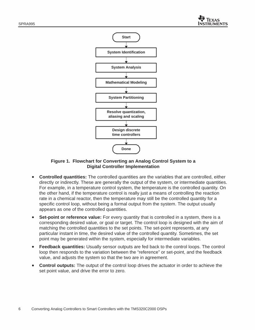
Converting a controller to an analog controller is best accomplished in a well-organized manner.Sections 3.1 through 3.8 outline the procedure to achieve this conversion. Also, Figure 1provides a flowchart of this procedure.

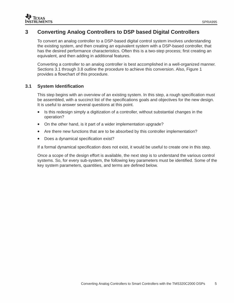
3.1 System Identification

This step begins with an overview of an existing system. In this step, a rough specification mustbe assembled, with a succinct list of the specifications goals and objectives for the new design.It is useful to answer several questions at this point.

• Is this redesign simply a digitization of a controller, without substantial changes in theoperation?

• On the other hand, is it part of a wider implementation upgrade?

• Are there new functions that are to be absorbed by this controller implementation?

• Does a dynamical specification exist?

If a formal dynamical specification does not exist, it would be useful to create one in this step.

Once a scope of the design effort is available, the next step is to understand the various controlsystems. So, for every sub-system, the following key parameters must be identified. Some of thekey system parameters, quantities, and terms are defined below.

SPRA995


Start

System Identification

System Analysis

Mathematical Modeling

System Partitioning

Resolve quantization,aliasing and scaling

Design discretetime controllers

Done

Figure 1. Flowchart for Converting an Analog Control System to aDigital Controller Implementation

• Controlled quantities: The controlled quantities are the variables that are controlled, eitherdirectly or indirectly. These are generally the output of the system, or intermediate quantities.For example, in a temperature control system, the temperature is the controlled quantity. Onthe other hand, if the temperature control is really just a means of controlling the reactionrate in a chemical reactor, then the temperature may still be the controlled quantity for aspecific control loop, without being a formal output from the system. The output usuallyappears as one of the controlled quantities.

• Set-point or reference value: For every quantity that is controlled in a system, there is acorresponding desired value, or goal or target. The control loop is designed with the aim ofmatching the controlled quantities to the set points. The set-point represents, at anyparticular instant in time, the desired value of the controlled quantity. Sometimes, the setpoint may be generated within the system, especially for intermediate variables.

• Feedback quantities: Usually sensor outputs are fed back to the control loops. The controlloop then responds to the variation between the “reference” or set-point, and the feedbackvalue, and adjusts the system so that the two are in agreement.

• Control outputs: The output of the control loop drives the actuator in order to achieve theset point value, and drive the error to zero.

SPRA995


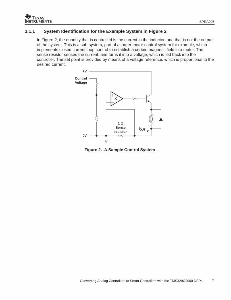
3.1.1 System Identification for the Example System in Figure 2

In Figure 2, the quantity that is controlled is the current in the inductor, and that is not the outputof the system. This is a sub-system, part of a larger motor control system for example, whichimplements closed current loop control to establish a certain magnetic field in a motor. Thesense resistor senses the current, and turns it into a voltage, which is fed back into thecontroller. The set point is provided by means of a voltage reference, which is proportional to thedesired current.

K

+V

0V

ControlVoltage

IOUT

1 Sense

resistor

Figure 2. A Sample Control System

SPRA995


0 V

IOUT

Comp Driver

Sawtoothgenerator

0−1 V

Output Amplifier

Plant

K=10ControllerOutputu

Feedback

0.1

Sensor Senseresistor

“SetPoint”

+100 V

Controller

x

Outputy

r0−1 V

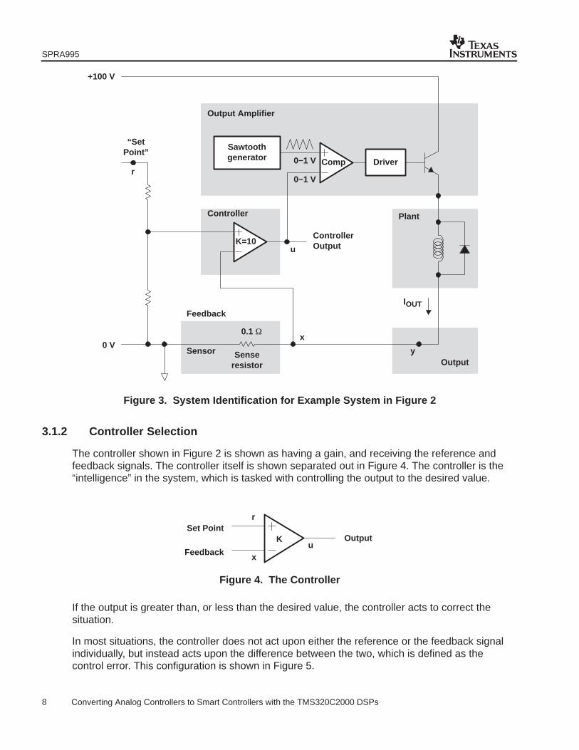
Figure 3. System Identification for Example System in Figure 2

3.1.2 Controller Selection

The controller shown in Figure 2 is shown as having a gain, and receiving the reference andfeedback signals. The controller itself is shown separated out in Figure 4. The controller is the“intelligence” in the system, which is tasked with controlling the output to the desired value.

KSet Point

Feedback

r

x

Outputu

Figure 4. The Controller

If the output is greater than, or less than the desired value, the controller acts to correct thesituation.

In most situations, the controller does not act upon either the reference or the feedback signalindividually, but instead acts upon the difference between the two, which is defined as thecontrol error. This configuration is shown in Figure 5.

SPRA995


Controller

e r x

u

x

r e

Figure 5. Error Based Control

Various control topologies are possible. For a review of various controller topologies, see 1-4listed in the Reference section of this application report as a useful source of various possibleconfigurations.

3.1.3 What Goes Inside that Box Marked “Controller”?

The controller creates the control output to accomplish the goal, which is to drive the controlledvariable to the desired value. Various mathematical relationships are used to derive the outputfrom the error value. Such a mathematical relationship is known as a control law. A control lawdescribes the relationship between the set point, feedback value, and the output of thecontroller.

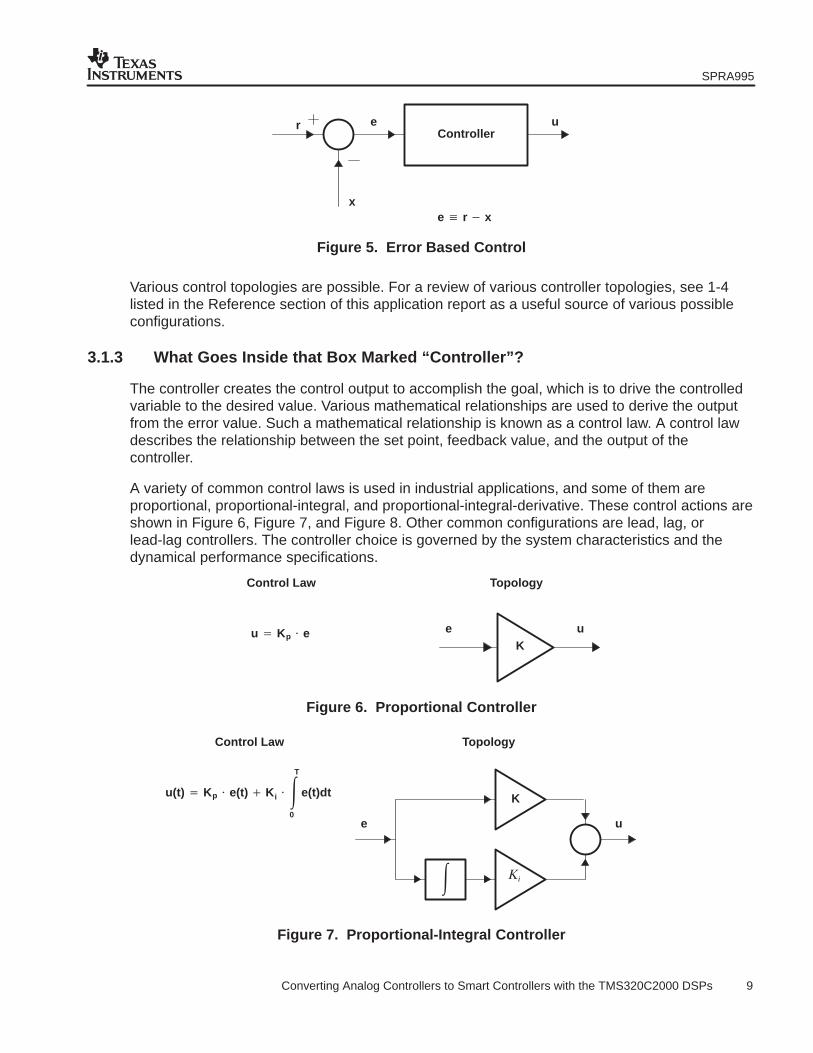
A variety of common control laws is used in industrial applications, and some of them areproportional, proportional-integral, and proportional-integral-derivative. These control actions areshown in Figure 6, Figure 7, and Figure 8. Other common configurations are lead, lag, orlead-lag controllers. The controller choice is governed by the system characteristics and thedynamical performance specifications.

Ke u

TopologyControl Law

u Kp e

Figure 6. Proportional Controller

K

e u

TopologyControl Law

u(t) Kp e(t) Ki T

0

e(t)dt

Figure 7. Proportional-Integral Controller

SPRA995


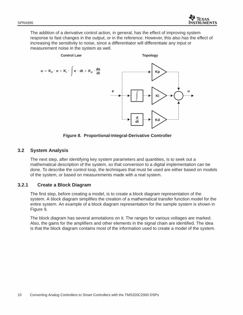
The addition of a derivative control action, in general, has the effect of improving systemresponse to fast changes in the output, or in the reference. However, this also has the effect ofincreasing the sensitivity to noise, since a differentiator will differentiate any input ormeasurement noise in the system as well.

Kp

e u

TopologyControl Law

u Kp e Ki e dt Kd dedt

Ki

Kdddt

Figure 8. Proportional-Integral-Derivative Controller

3.2 System Analysis

The next step, after identifying key system parameters and quantities, is to seek out amathematical description of the system, so that conversion to a digital implementation can bedone. To describe the control loop, the techniques that must be used are either based on modelsof the system, or based on measurements made with a real system.

3.2.1 Create a Block Diagram

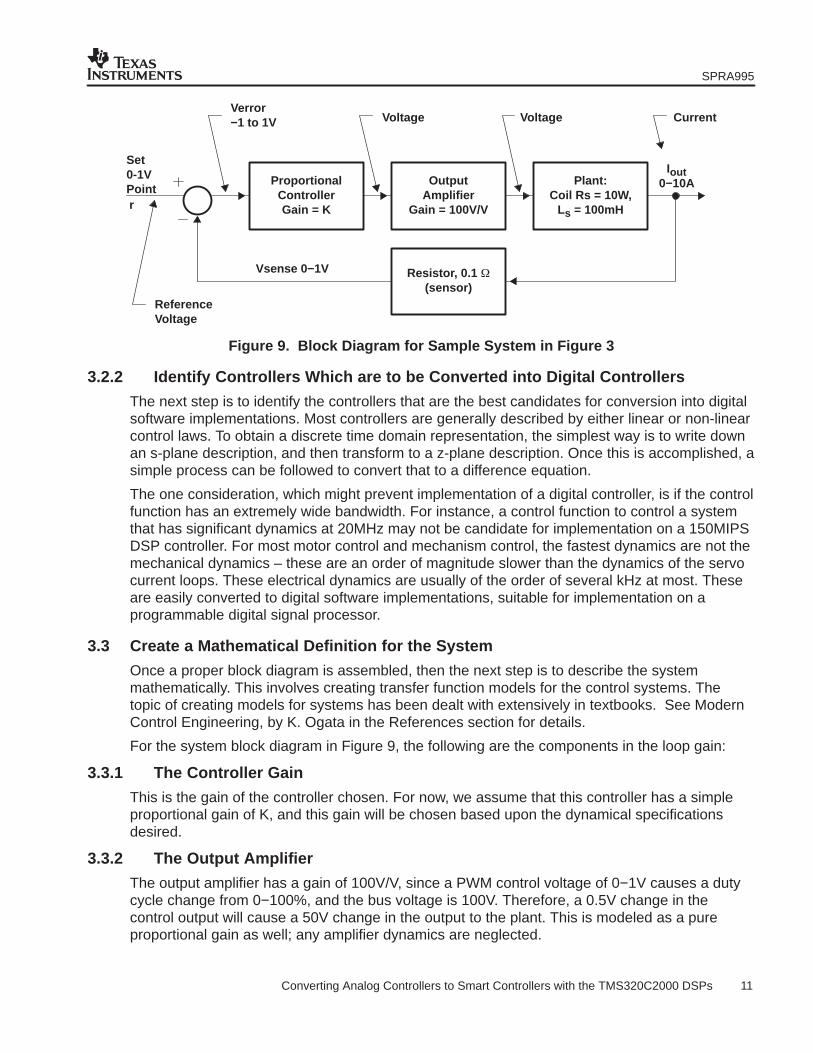
The first step, before creating a model, is to create a block diagram representation of thesystem. A block diagram simplifies the creation of a mathematical transfer function model for theentire system. An example of a block diagram representation for the sample system is shown inFigure 9.

The block diagram has several annotations on it. The ranges for various voltages are marked.Also, the gains for the amplifiers and other elements in the signal chain are identified. The ideais that the block diagram contains most of the information used to create a model of the system.

SPRA995


ProportionalControllerGain = K

Set0-1VPointr

OutputAmplifier

Gain = 100V/V

Plant:Coil Rs = 10W,

Ls = 100mH

Resistor, 0.1 (sensor)

Iout0−10A

Vsense 0−1V

Verror−1 to 1V Voltage

ReferenceVoltage

Voltage Current

Figure 9. Block Diagram for Sample System in Figure 3

3.2.2 Identify Controllers Which are to be Converted into Digital Controllers

The next step is to identify the controllers that are the best candidates for conversion into digitalsoftware implementations. Most controllers are generally described by either linear or non-linearcontrol laws. To obtain a discrete time domain representation, the simplest way is to write downan s-plane description, and then transform to a z-plane description. Once this is accomplished, asimple process can be followed to convert that to a difference equation.

The one consideration, which might prevent implementation of a digital controller, is if the controlfunction has an extremely wide bandwidth. For instance, a control function to control a systemthat has significant dynamics at 20MHz may not be candidate for implementation on a 150MIPSDSP controller. For most motor control and mechanism control, the fastest dynamics are not themechanical dynamics – these are an order of magnitude slower than the dynamics of the servocurrent loops. These electrical dynamics are usually of the order of several kHz at most. Theseare easily converted to digital software implementations, suitable for implementation on aprogrammable digital signal processor.

3.3 Create a Mathematical Definition for the System

Once a proper block diagram is assembled, then the next step is to describe the systemmathematically. This involves creating transfer function models for the control systems. Thetopic of creating models for systems has been dealt with extensively in textbooks. See ModernControl Engineering, by K. Ogata in the References section for details.

For the system block diagram in Figure 9, the following are the components in the loop gain:

3.3.1 The Controller Gain

This is the gain of the controller chosen. For now, we assume that this controller has a simpleproportional gain of K, and this gain will be chosen based upon the dynamical specificationsdesired.

3.3.2 The Output Amplifier

The output amplifier has a gain of 100V/V, since a PWM control voltage of 0−1V causes a dutycycle change from 0−100%, and the bus voltage is 100V. Therefore, a 0.5V change in thecontrol output will cause a 50V change in the output to the plant. This is modeled as a pureproportional gain as well; any amplifier dynamics are neglected.

SPRA995


3.3.3 Plant Transfer Function

The plant is an R-L model for a simple coil, and the coil transfer function may be modeled asfollows:

V(t)L i(t) R L

di(t)dt

This equation can be transformed via the Laplace transform, and that gives an algebraicequation, which can be written as:

V(s) I(s) R L sI(s)

Rearranging as a transfer function we have:

I(s)V(s)

1L

s Rl

I(s)V(s)

10s 100

Now, we substitute values for the constants R=10Ω and L=100mH, and have:

This is a so-called s-domain transfer function, and is very useful to model the plant. The planthas a simple pole at s= –100 and has a DC gain of 0.1. The output of the plant is current inamperes, and input is voltage in volts.

3.3.4 Sensor Gain

The output of the plant is converted into a voltage, so that it may be fed back to the control loop.In our case, the sensor is simply a resistor. Depending upon various application considerations,it could be a Hall Effect sensor, or a current transformer with a resistor in the secondary. To us,for now, it is more interesting to know that the mathematical description of this “current to voltageconverter” – is governed by the following relationship (Ohm’s law):

V I R

Thus the gain of the sensor is simply the resistance, and is 0.1 Volts per ampere.

3.3.5 Loop Gain

From a control system point of view, the description for the various system components is nowcompiled into the loop gain, and for our example system we may write the loop gain G(s) as:

G(s) (K) (100) (0.1) 10s 100

This may be then boiled down a little into the following form

G(s) K 100s 100

Equation (6) is a very important way of describing our system from a dynamical point of view. Itrepresents all the gains and dynamics in the system, and allows the usage of several designtechniques such as root locus, bode diagrams etc. for controller design. Once the controller hasbeen designed, then the next step involves realizing the control system.

(1)

(2)

(3)

(4)

(5)

(6)

SPRA995


3.4 Partition the System into Hardware Components and Software Components

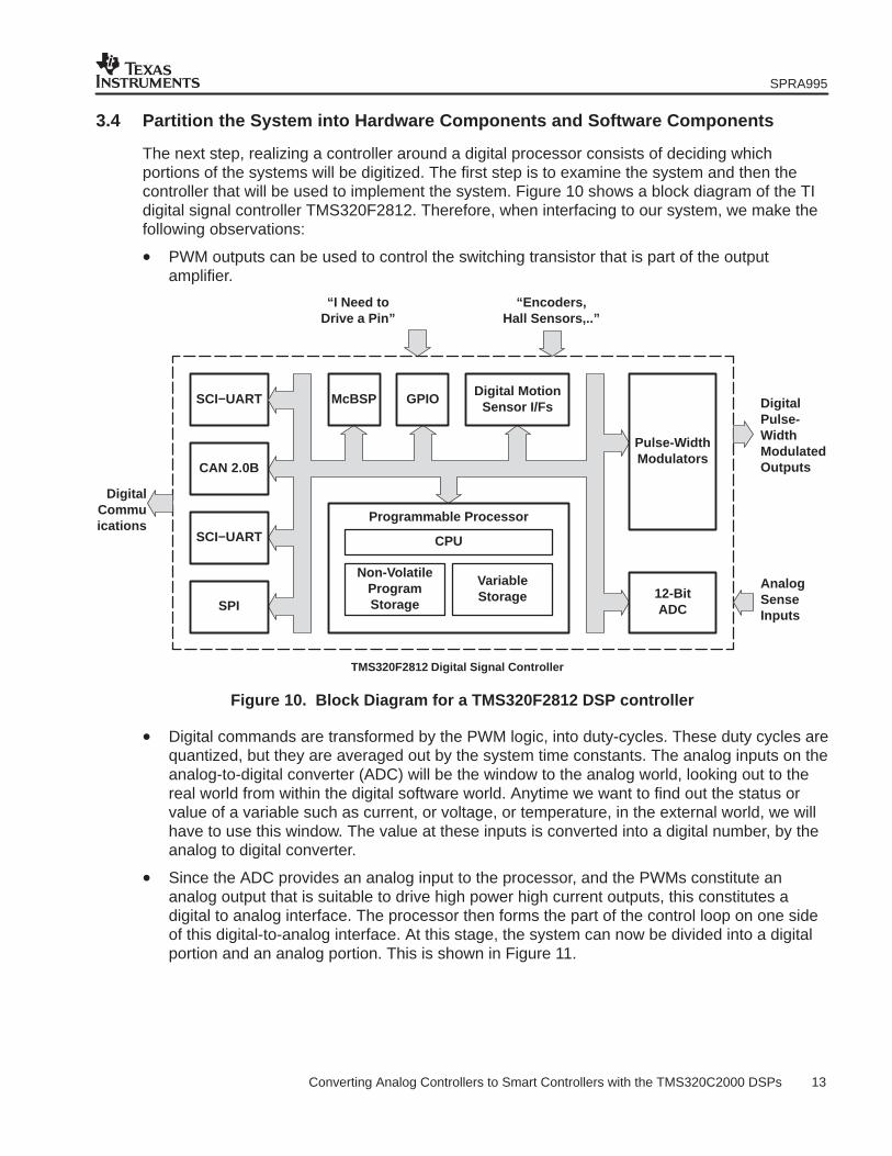
The next step, realizing a controller around a digital processor consists of deciding whichportions of the systems will be digitized. The first step is to examine the system and then thecontroller that will be used to implement the system. Figure 10 shows a block diagram of the TIdigital signal controller TMS320F2812. Therefore, when interfacing to our system, we make thefollowing observations:

• PWM outputs can be used to control the switching transistor that is part of the outputamplifier.

SCI−UART

CAN 2.0B

SPI

SCI−UART

Digital MotionSensor I/Fs

GPIOMcBSP

Pulse-WidthModulators

12-BitADC

Programmable Processor

CPU

Non-VolatileProgramStorage

VariableStorage

“I Need toDrive a Pin”

“Encoders,Hall Sensors,..”

DigitalPulse-WidthModulate dOutputs

AnalogSenseInputs

DigitalCommuications

TMS320F2812 Digital Signal Controller

Figure 10. Block Diagram for a TMS320F2812 DSP controller

• Digital commands are transformed by the PWM logic, into duty-cycles. These duty cycles arequantized, but they are averaged out by the system time constants. The analog inputs on theanalog-to-digital converter (ADC) will be the window to the analog world, looking out to thereal world from within the digital software world. Anytime we want to find out the status orvalue of a variable such as current, or voltage, or temperature, in the external world, we willhave to use this window. The value at these inputs is converted into a digital number, by theanalog to digital converter.

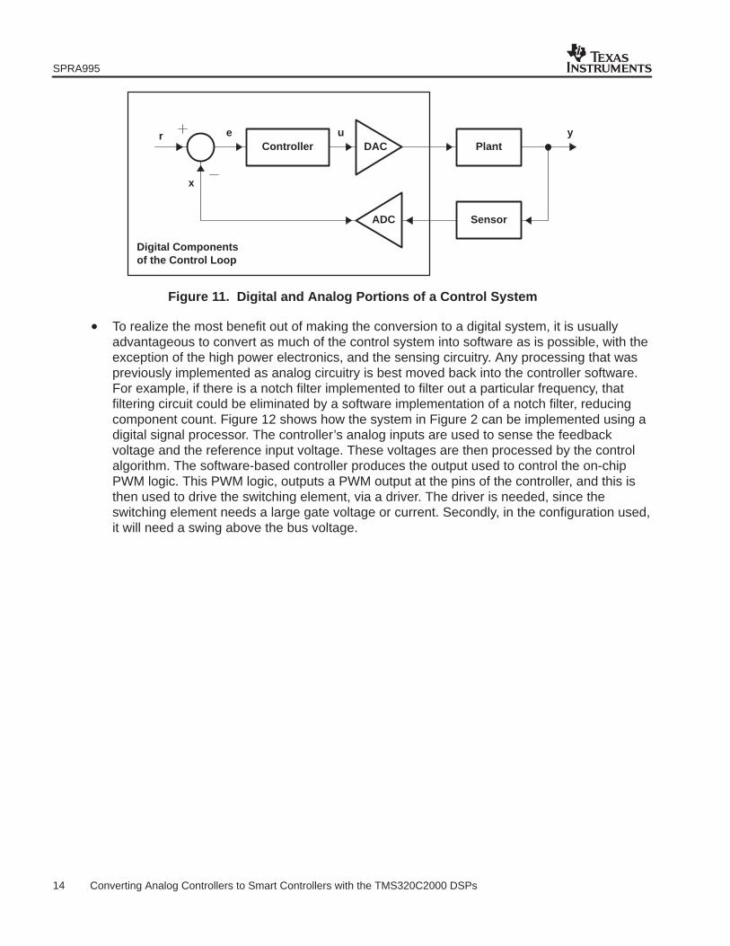
• Since the ADC provides an analog input to the processor, and the PWMs constitute ananalog output that is suitable to drive high power high current outputs, this constitutes adigital to analog interface. The processor then forms the part of the control loop on one sideof this digital-to-analog interface. At this stage, the system can now be divided into a digitalportion and an analog portion. This is shown in Figure 11.

SPRA995


DACe

ADC

Plant

Sensor

yController

r

x

u

Digital Componentsof the Control Loop

Figure 11. Digital and Analog Portions of a Control System

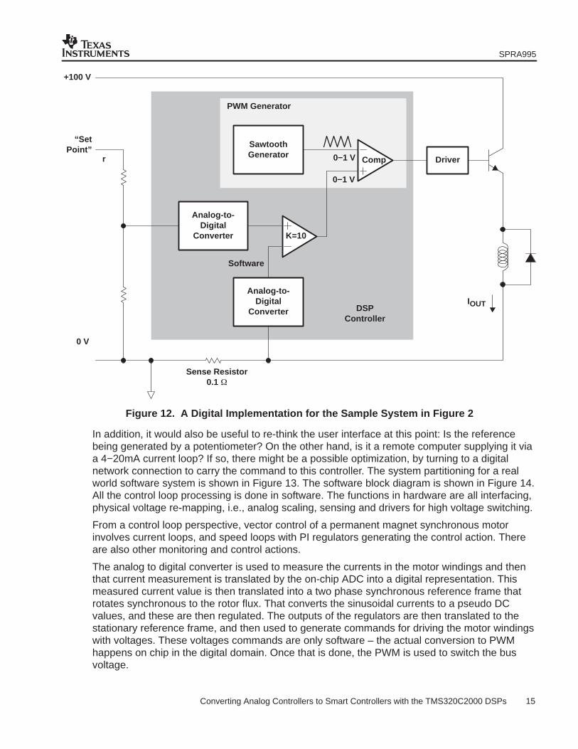
• To realize the most benefit out of making the conversion to a digital system, it is usuallyadvantageous to convert as much of the control system into software as is possible, with theexception of the high power electronics, and the sensing circuitry. Any processing that waspreviously implemented as analog circuitry is best moved back into the controller software.For example, if there is a notch filter implemented to filter out a particular frequency, thatfiltering circuit could be eliminated by a software implementation of a notch filter, reducingcomponent count. Figure 12 shows how the system in Figure 2 can be implemented using adigital signal processor. The controller’s analog inputs are used to sense the feedbackvoltage and the reference input voltage. These voltages are then processed by the controlalgorithm. The software-based controller produces the output used to control the on-chipPWM logic. This PWM logic, outputs a PWM output at the pins of the controller, and this isthen used to drive the switching element, via a driver. The driver is needed, since theswitching element needs a large gate voltage or current. Secondly, in the configuration used,it will need a swing above the bus voltage.

SPRA995


0 V

IOUT

Comp Driver

SawtoothGenerator 0−1 V

0−1 V

K=10

Sense Resistor0.1

“SetPoint”

+100 V

r

Analog-to-Digital

Converter

PWM Generator

DSPController

Software

Analog-to-Digital

Converter

Figure 12. A Digital Implementation for the Sample System in Figure 2

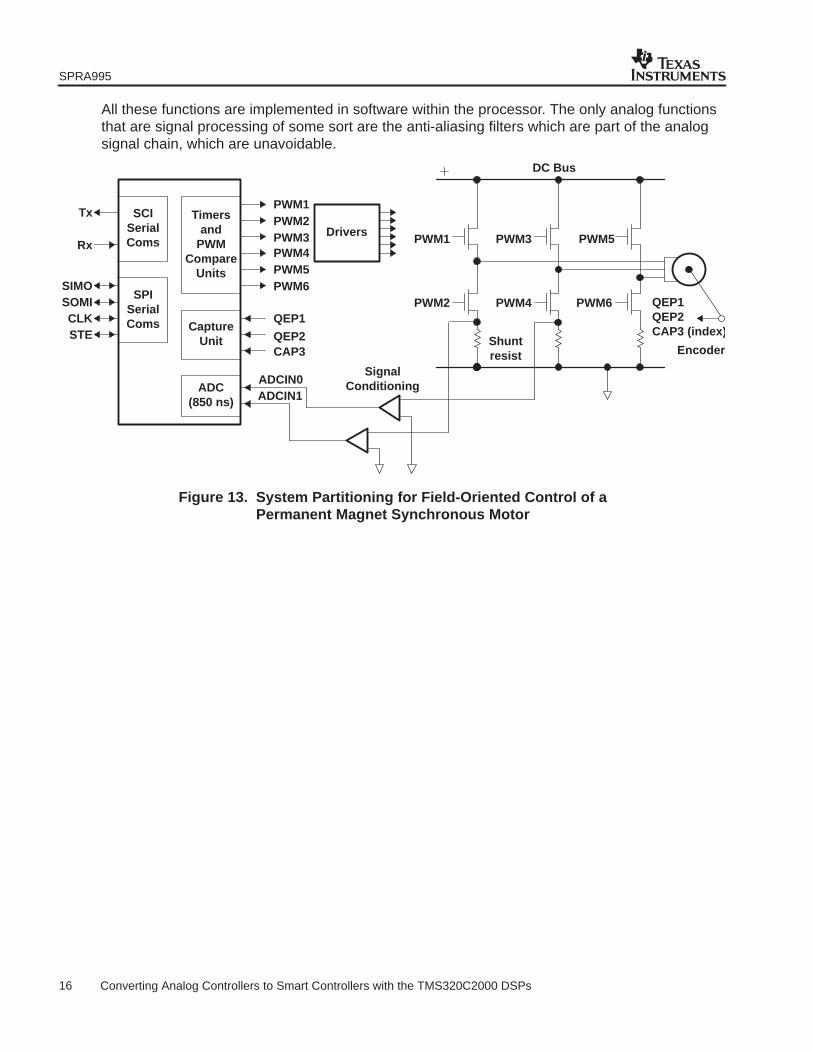
In addition, it would also be useful to re-think the user interface at this point: Is the referencebeing generated by a potentiometer? On the other hand, is it a remote computer supplying it viaa 4−20mA current loop? If so, there might be a possible optimization, by turning to a digitalnetwork connection to carry the command to this controller. The system partitioning for a realworld software system is shown in Figure 13. The software block diagram is shown in Figure 14.All the control loop processing is done in software. The functions in hardware are all interfacing,physical voltage re-mapping, i.e., analog scaling, sensing and drivers for high voltage switching.

From a control loop perspective, vector control of a permanent magnet synchronous motorinvolves current loops, and speed loops with PI regulators generating the control action. Thereare also other monitoring and control actions.

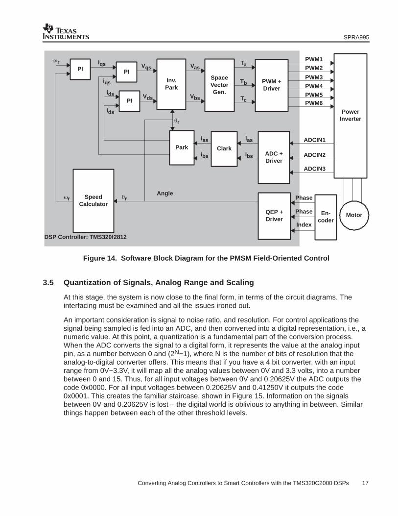
The analog to digital converter is used to measure the currents in the motor windings and thenthat current measurement is translated by the on-chip ADC into a digital representation. Thismeasured current value is then translated into a two phase synchronous reference frame thatrotates synchronous to the rotor flux. That converts the sinusoidal currents to a pseudo DCvalues, and these are then regulated. The outputs of the regulators are then translated to thestationary reference frame, and then used to generate commands for driving the motor windingswith voltages. These voltages commands are only software – the actual conversion to PWMhappens on chip in the digital domain. Once that is done, the PWM is used to switch the busvoltage.

SPRA995


All these functions are implemented in software within the processor. The only analog functionsthat are signal processing of some sort are the anti-aliasing filters which are part of the analogsignal chain, which are unavoidable.

SCISerialComs

Tx

Rx

SIMOSOMI

STECLK

Timersand

PWMCompare

Units

CaptureUnit

ADC(850 ns)

PWM1

QEP1

ADCIN0ADCIN1

Drivers

DC Bus

QEP1QEP2CAP3 (inde x)

Shuntresist

SignalConditioning

SPISerialComs

PWM2PWM3PWM4PWM5PWM6

QEP2CAP3

PWM1

PWM2

PWM3 PWM5

PWM4 PWM6

Encod er

Figure 13. System Partitioning for Field-Oriented Control of aPermanent Magnet Synchronous Motor

SPRA995


Motor

Park

PI

Clark

PWM1

ADCIN1

AnglePhase

Inv.Park

SpaceVectorGen.

SpeedCalculator

ADC +Driver

PWM +Driver

PowerInverter

En-coder

PWM2

PWM3

PWM4

PWM5PWM6

ADCIN2

ADCIN3

Phase

Index

PIPIr

r r

r

iqs

Vds

iqs

ids

ids

Vqs

Vbs

VasTa

Tb

Tc

ibs

ias

ibs

ias

QEP +Driver

DSP Controller: TMS320f2812

Figure 14. Software Block Diagram for the PMSM Field-Oriented Control

3.5 Quantization of Signals, Analog Range and Scaling

At this stage, the system is now close to the final form, in terms of the circuit diagrams. Theinterfacing must be examined and all the issues ironed out.

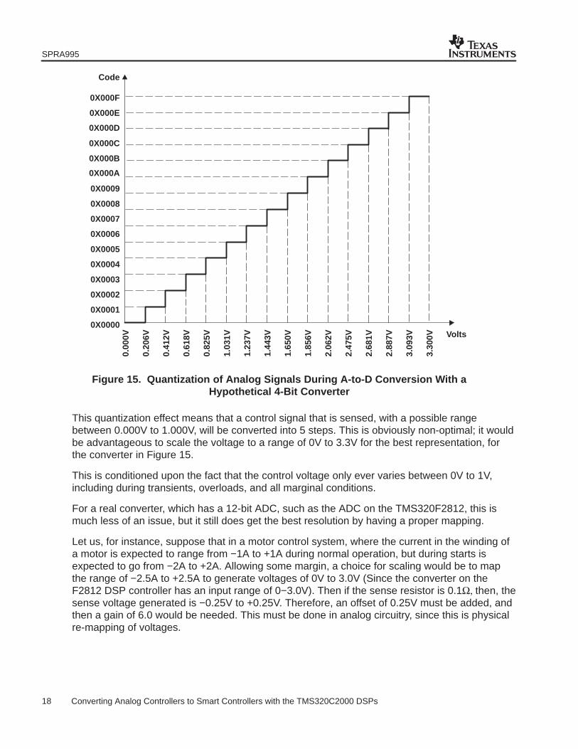
An important consideration is signal to noise ratio, and resolution. For control applications thesignal being sampled is fed into an ADC, and then converted into a digital representation, i.e., anumeric value. At this point, a quantization is a fundamental part of the conversion process.When the ADC converts the signal to a digital form, it represents the value at the analog inputpin, as a number between 0 and (2N−1), where N is the number of bits of resolution that theanalog-to-digital converter offers. This means that if you have a 4 bit converter, with an inputrange from 0V−3.3V, it will map all the analog values between 0V and 3.3 volts, into a numberbetween 0 and 15. Thus, for all input voltages between 0V and 0.20625V the ADC outputs thecode 0x0000. For all input voltages between 0.20625V and 0.41250V it outputs the code0x0001. This creates the familiar staircase, shown in Figure 15. Information on the signalsbetween 0V and 0.20625V is lost – the digital world is oblivious to anything in between. Similarthings happen between each of the other threshold levels.

SPRA995


0X000B

0X0000

0X0001

0X0002

0X0003

0X0004

0X0005

0X0006

0X0007

0X0008

0X0009

0X000A

0X000C

0X000D

0X000E

0X000F

Volts

Code

0.00

0V

0.20

6V

0.41

2V

0.61

8V

0.82

5V

1.03

1V

1.23

7V

1.44

3V

1.65

0V

1.85

6V

2.06

2V

2.47

5V

2.68

1V

2.88

7V

3.09

3V

3.30

0V

Figure 15. Quantization of Analog Signals During A-to-D Conversion With aHypothetical 4-Bit Converter

This quantization effect means that a control signal that is sensed, with a possible rangebetween 0.000V to 1.000V, will be converted into 5 steps. This is obviously non-optimal; it wouldbe advantageous to scale the voltage to a range of 0V to 3.3V for the best representation, forthe converter in Figure 15.

This is conditioned upon the fact that the control voltage only ever varies between 0V to 1V,including during transients, overloads, and all marginal conditions.

For a real converter, which has a 12-bit ADC, such as the ADC on the TMS320F2812, this ismuch less of an issue, but it still does get the best resolution by having a proper mapping.

Let us, for instance, suppose that in a motor control system, where the current in the winding ofa motor is expected to range from −1A to +1A during normal operation, but during starts isexpected to go from −2A to +2A. Allowing some margin, a choice for scaling would be to mapthe range of −2.5A to +2.5A to generate voltages of 0V to 3.0V (Since the converter on theF2812 DSP controller has an input range of 0−3.0V). Then if the sense resistor is 0.1Ω, then, thesense voltage generated is −0.25V to +0.25V. Therefore, an offset of 0.25V must be added, andthen a gain of 6.0 would be needed. This must be done in analog circuitry, since this is physicalre-mapping of voltages.

SPRA995


3.6 Anti-Aliasing Considerations

A phenomenon that is introduced into a control system, as a direct consequence of the samplingprocess, is aliasing. Aliasing can cause a number of undesirable effects, and is undesired mostof the time.

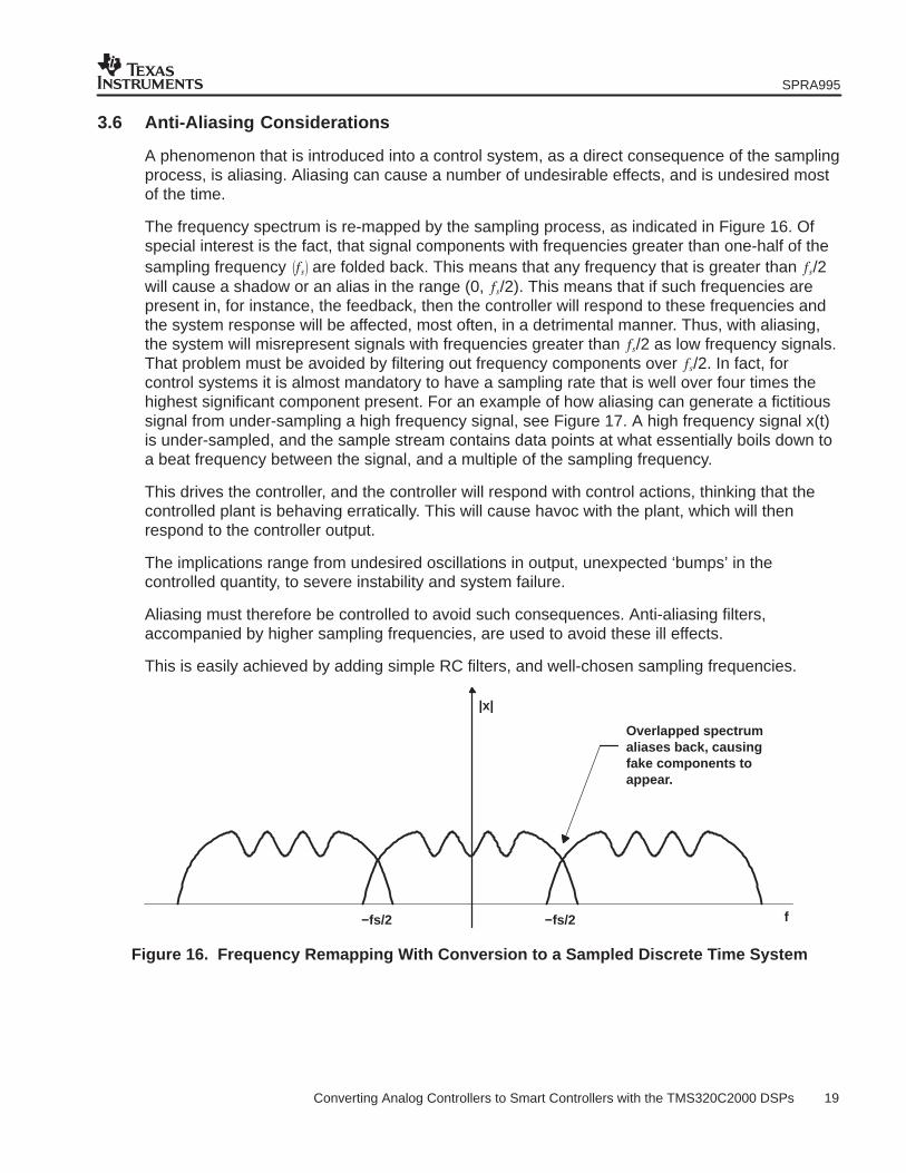
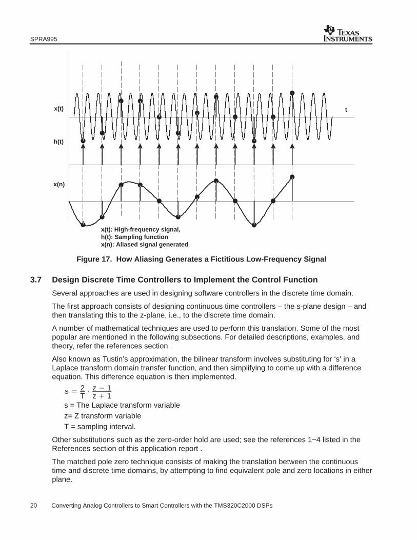
The frequency spectrum is re-mapped by the sampling process, as indicated in Figure 16. Ofspecial interest is the fact, that signal components with frequencies greater than one-half of thesampling frequency are folded back. This means that any frequency that is greater than /2will cause a shadow or an alias in the range (0, /2). This means that if such frequencies arepresent in, for instance, the feedback, then the controller will respond to these frequencies andthe system response will be affected, most often, in a detrimental manner. Thus, with aliasing,the system will misrepresent signals with frequencies greater than /2 as low frequency signals.That problem must be avoided by filtering out frequency components over /2. In fact, forcontrol systems it is almost mandatory to have a sampling rate that is well over four times thehighest significant component present. For an example of how aliasing can generate a fictitioussignal from under-sampling a high frequency signal, see Figure 17. A high frequency signal x(t)is under-sampled, and the sample stream contains data points at what essentially boils down toa beat frequency between the signal, and a multiple of the sampling frequency.

This drives the controller, and the controller will respond with control actions, thinking that thecontrolled plant is behaving erratically. This will cause havoc with the plant, which will thenrespond to the controller output.

The implications range from undesired oscillations in output, unexpected ‘bumps’ in thecontrolled quantity, to severe instability and system failure.

Aliasing must therefore be controlled to avoid such consequences. Anti-aliasing filters,accompanied by higher sampling frequencies, are used to avoid these ill effects.

This is easily achieved by adding simple RC filters, and well-chosen sampling frequencies.

|x|

Overlapped spectrumaliases back, causingfake components toappear.

−fs/2 −fs/2 f

Figure 16. Frequency Remapping With Conversion to a Sampled Discrete Time System

SPRA995


x(t)

h(t)

x(n)

x(t): High-frequency signal,h(t): Sampling functionx(n): Aliased signal generated

t

Figure 17. How Aliasing Generates a Fictitious Low-Frequency Signal

3.7 Design Discrete Time Controllers to Implement the Control Function

Several approaches are used in designing software controllers in the discrete time domain.

The first approach consists of designing continuous time controllers – the s-plane design – andthen translating this to the z-plane, i.e., to the discrete time domain.

A number of mathematical techniques are used to perform this translation. Some of the mostpopular are mentioned in the following subsections. For detailed descriptions, examples, andtheory, refer the references section.

Also known as Tustin’s approximation, the bilinear transform involves substituting for ‘s’ in aLaplace transform domain transfer function, and then simplifying to come up with a differenceequation. This difference equation is then implemented.

s 2T z 1

z 1s = The Laplace transform variablez= Z transform variableT = sampling interval.

Other substitutions such as the zero-order hold are used; see the references 1−4 listed in theReferences section of this application report .

The matched pole zero technique consists of making the translation between the continuoustime and discrete time domains, by attempting to find equivalent pole and zero locations in eitherplane.

SPRA995


Usually, the design of controls in the s-plane and translation to z-domain is a way to avoidredesigning a controller for translating an existing controller for implementation. However, theapproaches that deal with designing controllers in discrete time domain give the most flexibility.

There are also design techniques, such as dead-beat controllers, which are only available in thediscrete time domain.

Another approach, involving modeling the system as a state-space model, and converting themodel to discrete time state-model, allows the designer to exploit techniques such as stateobservers to reduce or eliminate sensors.

As mentioned at the outset, this application report does not attempt to supply descriptions of theactual mathematics of the conversion, since this topic is covered in many excellent text books onthe subject. Some of these are mentioned in the references section.

3.8 Choosing Sampling Rates in a Quantized Discrete Time Domain System

To discretize the controller, the designer must choose a sampling frequency that allows thedesigner to convert to a discrete form.

Obviously, the criterion for avoiding aliasing are important. However, in control systems, it isalmost always necessary to go far beyond the sampling rates suggested by the Nyquist criterion.

In choosing a sampling frequency, determine the highest frequency component that is present inthe system (ωH). Then the sampling frequency chosen must be greater two times this. Forexample,

s 2H

However, this does not usually allow the proper functioning of a control system. It is commonpractice to choose a frequency that is at least 4ωH, for first order systems. For higher ordersystems, e.g., second order systems, a common choice is a sampling rate that is 10 times fasterthan the highest frequency component present. This is driven by the requirements to keep theinter sample deviations to an acceptable minimum.

To illustrate this effect, Table 1 shows what happens to the controller coefficients as thesampling rate is changed.

For this example, a simple one pole transfer function is discretized.

The transfer function is

G(s) 100s 100

SPRA995


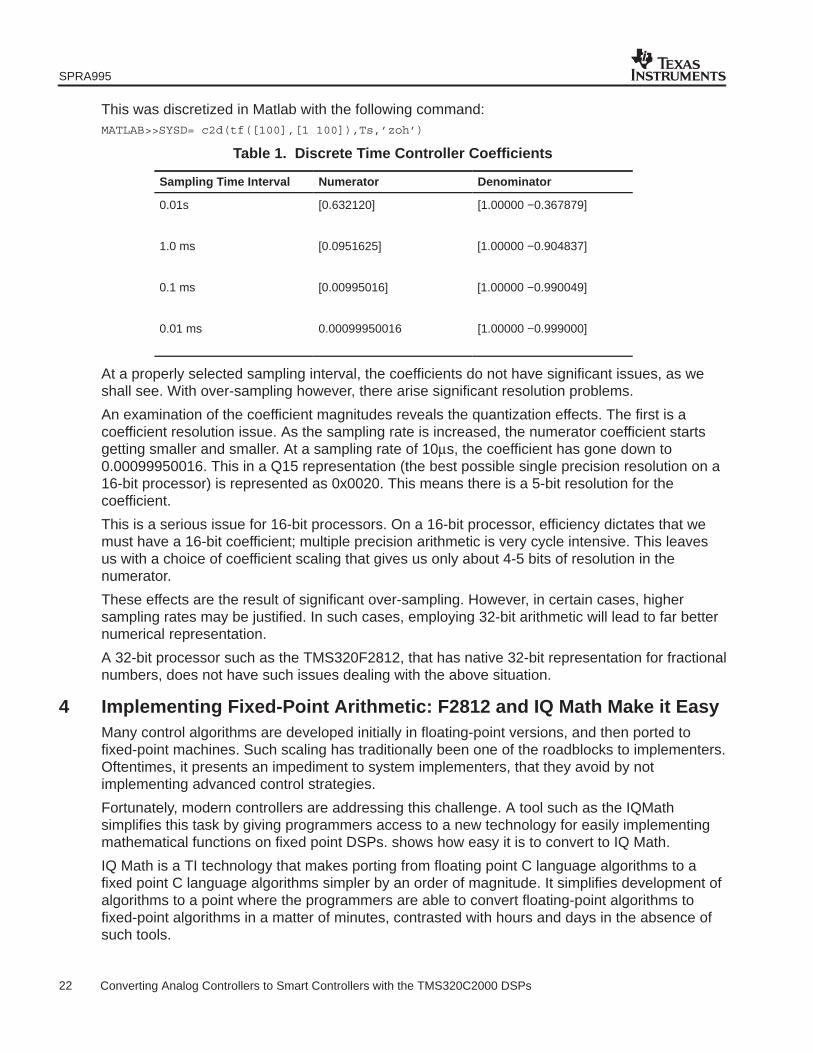
This was discretized in Matlab with the following command:MATLAB>>SYSD= c2d(tf([100],[1 100]),Ts,’zoh’)

Table 1. Discrete Time Controller Coefficients

Sampling Time Interval Numerator Denominator

0.01s [0.632120] [1.00000 −0.367879]

1.0 ms [0.0951625] [1.00000 −0.904837]

0.1 ms [0.00995016] [1.00000 −0.990049]

0.01 ms 0.00099950016 [1.00000 −0.999000]

At a properly selected sampling interval, the coefficients do not have significant issues, as weshall see. With over-sampling however, there arise significant resolution problems.

An examination of the coefficient magnitudes reveals the quantization effects. The first is acoefficient resolution issue. As the sampling rate is increased, the numerator coefficient startsgetting smaller and smaller. At a sampling rate of 10µs, the coefficient has gone down to0.00099950016. This in a Q15 representation (the best possible single precision resolution on a16-bit processor) is represented as 0x0020. This means there is a 5-bit resolution for thecoefficient.

This is a serious issue for 16-bit processors. On a 16-bit processor, efficiency dictates that wemust have a 16-bit coefficient; multiple precision arithmetic is very cycle intensive. This leavesus with a choice of coefficient scaling that gives us only about 4-5 bits of resolution in thenumerator.

These effects are the result of significant over-sampling. However, in certain cases, highersampling rates may be justified. In such cases, employing 32-bit arithmetic will lead to far betternumerical representation.

A 32-bit processor such as the TMS320F2812, that has native 32-bit representation for fractionalnumbers, does not have such issues dealing with the above situation.

4 Implementing Fixed-Point Arithmetic: F2812 and IQ Math Make it EasyMany control algorithms are developed initially in floating-point versions, and then ported tofixed-point machines. Such scaling has traditionally been one of the roadblocks to implementers.Oftentimes, it presents an impediment to system implementers, that they avoid by notimplementing advanced control strategies.

Fortunately, modern controllers are addressing this challenge. A tool such as the IQMathsimplifies this task by giving programmers access to a new technology for easily implementingmathematical functions on fixed point DSPs. shows how easy it is to convert to IQ Math.

IQ Math is a TI technology that makes porting from floating point C language algorithms to afixed point C language algorithms simpler by an order of magnitude. It simplifies development ofalgorithms to a point where the programmers are able to convert floating-point algorithms tofixed-point algorithms in a matter of minutes, contrasted with hours and days in the absence ofsuch tools.

SPRA995


The key concept behind IQ Math is to scale everything back to a global fixed-point format, sothat the conversion process to a fixed-point form becomes a mechanical process, which can beorganized as a series of well-defined steps.

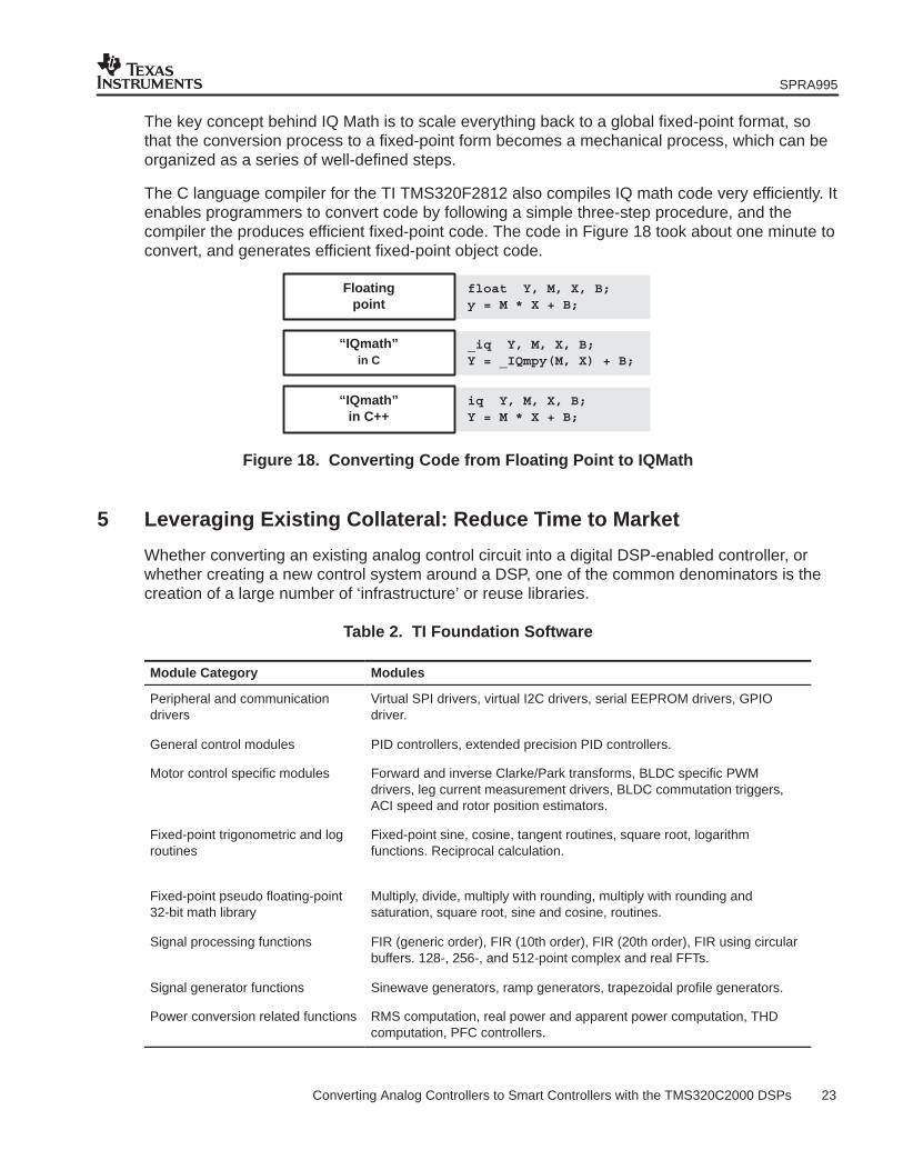
The C language compiler for the TI TMS320F2812 also compiles IQ math code very efficiently. Itenables programmers to convert code by following a simple three-step procedure, and thecompiler the produces efficient fixed-point code. The code in Figure 18 took about one minute toconvert, and generates efficient fixed-point object code.

Floatingpoint

“IQmath”in C

“IQmath”in C++

float Y, M, X, B;y = M * X + B;

_iq Y, M, X, B;Y = _IQmpy(M, X) + B;

iq Y, M, X, B;Y = M * X + B;

Figure 18. Converting Code from Floating Point to IQMath

5 Leveraging Existing Collateral: Reduce Time to Market

Whether converting an existing analog control circuit into a digital DSP-enabled controller, orwhether creating a new control system around a DSP, one of the common denominators is thecreation of a large number of ‘infrastructure’ or reuse libraries.

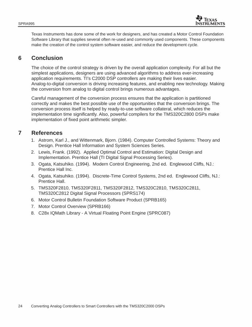
Table 2. TI Foundation Software

Module Category Modules

Peripheral and communicationdrivers

Virtual SPI drivers, virtual I2C drivers, serial EEPROM drivers, GPIOdriver.

General control modules PID controllers, extended precision PID controllers.

Motor control specific modules Forward and inverse Clarke/Park transforms, BLDC specific PWMdrivers, leg current measurement drivers, BLDC commutation triggers,ACI speed and rotor position estimators.

Fixed-point trigonometric and logroutines

Fixed-point sine, cosine, tangent routines, square root, logarithmfunctions. Reciprocal calculation.

Fixed-point pseudo floating-point32-bit math library

Multiply, divide, multiply with rounding, multiply with rounding andsaturation, square root, sine and cosine, routines.

Signal processing functions FIR (generic order), FIR (10th order), FIR (20th order), FIR using circularbuffers. 128-, 256-, and 512-point complex and real FFTs.

Signal generator functions Sinewave generators, ramp generators, trapezoidal profile generators.

Power conversion related functions RMS computation, real power and apparent power computation, THDcomputation, PFC controllers.

SPRA995


Texas Instruments has done some of the work for designers, and has created a Motor Control FoundationSoftware Library that supplies several often re-used and commonly used components. These componentsmake the creation of the control system software easier, and reduce the development cycle.

6 Conclusion

The choice of the control strategy is driven by the overall application complexity. For all but thesimplest applications, designers are using advanced algorithms to address ever-increasingapplication requirements. TI’s C2000 DSP controllers are making their lives easier.Analog-to-digital conversion is driving increasing features, and enabling new technology. Makingthe conversion from analog to digital control brings numerous advantages.

Careful management of the conversion process ensures that the application is partitionedcorrectly and makes the best possible use of the opportunities that the conversion brings. Theconversion process itself is helped by ready-to-use software collateral, which reduces theimplementation time significantly. Also, powerful compilers for the TMS320C2800 DSPs makeimplementation of fixed point arithmetic simpler.

7 References1. Astrom, Karl J., and Wittenmark, Bjorn. (1984). Computer Controlled Systems: Theory and

Design. Prentice Hall Information and System Sciences Series.

2. Lewis, Frank. (1992). Applied Optimal Control and Estimation: Digital Design andImplementation. Prentice Hall (TI Digital Signal Processing Series).

3. Ogata, Katsuhiko. (1994). Modern Control Engineering, 2nd ed. Englewood Cliffs, NJ.:Prentice Hall Inc.

4. Ogata, Katsuhiko. (1994). Discrete-Time Control Systems, 2nd ed. Englewood Cliffs, NJ.:Prentice Hall.

5. TMS320F2810, TMS320F2811, TMS320F2812, TMS320C2810, TMS320C2811,TMS320C2812 Digital Signal Processors (SPRS174)

6. Motor Control Bulletin Foundation Software Product (SPRB165)

7. Motor Control Overview (SPRB166)

8. C28x IQMath Library - A Virtual Floating Point Engine (SPRC087)

IMPORTANT NOTICE

Texas Instruments Incorporated and its subsidiaries (TI) reserve the right to make corrections, modifications,enhancements, improvements, and other changes to its products and services at any time and to discontinueany product or service without notice. Customers should obtain the latest relevant information before placingorders and should verify that such information is current and complete. All products are sold subject to TI’s termsand conditions of sale supplied at the time of order acknowledgment.

TI warrants performance of its hardware products to the specifications applicable at the time of sale inaccordance with TI’s standard warranty. Testing and other quality control techniques are used to the extent TIdeems necessary to support this warranty. Except where mandated by government requirements, testing of allparameters of each product is not necessarily performed.

TI assumes no liability for applications assistance or customer product design. Customers are responsible fortheir products and applications using TI components. To minimize the risks associated with customer productsand applications, customers should provide adequate design and operating safeguards.

TI does not warrant or represent that any license, either express or implied, is granted under any TI patent right,copyright, mask work right, or other TI intellectual property right relating to any combination, machine, or processin which TI products or services are used. Information published by TI regarding third-party products or servicesdoes not constitute a license from TI to use such products or services or a warranty or endorsement thereof.Use of such information may require a license from a third party under the patents or other intellectual propertyof the third party, or a license from TI under the patents or other intellectual property of TI.

Reproduction of information in TI data books or data sheets is permissible only if reproduction is withoutalteration and is accompanied by all associated warranties, conditions, limitations, and notices. Reproductionof this information with alteration is an unfair and deceptive business practice. TI is not responsible or liable forsuch altered documentation.

Resale of TI products or services with statements different from or beyond the parameters stated by TI for thatproduct or service voids all express and any implied warranties for the associated TI product or service andis an unfair and deceptive business practice. TI is not responsible or liable for any such statements.

Following are URLs where you can obtain information on other Texas Instruments products and applicationsolutions:

Products Applications

Amplifiers amplifier.ti.com Audio www.ti.com/audio

Data Converters dataconverter.ti.com Automotive www.ti.com/automotive

DSP dsp.ti.com Broadband www.ti.com/broadband

Interface interface.ti.com Digital Control www.ti.com/digitalcontrol

Logic logic.ti.com Military www.ti.com/military

Power Mgmt power.ti.com Optical Networking www.ti.com/opticalnetwork

Microcontrollers microcontroller.ti.com Security www.ti.com/security

Telephony www.ti.com/telephony

Video & Imaging www.ti.com/video

Wireless www.ti.com/wireless

Mailing Address: Texas Instruments

Post Office Box 655303 Dallas, Texas 75265

Copyright 2004, Texas Instruments Incorporated

http://amplifier.ti.com

http://dataconverter.ti.com

http://dsp.ti.com

http://interface.ti.com

http://logic.ti.com

http://power.ti.com

http://microcontroller.ti.com

http://www.ti.com/audio

http://www.ti.com/automotive

http://www.ti.com/broadband

http://www.ti.com/digitalcontrol

http://www.ti.com/military

http://www.ti.com/opticalnetwork

http://www.ti.com/security

http://www.ti.com/telephony

http://www.ti.com/video

http://www.ti.com/wireless

Documents

Converting Analog Controllers to Smart Controllers with ... · SPRA995 4 Converting Analog Controllers to Smart Controllers with the TMS320C2000 DSPs • Ease of implementation: Functions