HAL Id: hal-00720617https://hal.archives-ouvertes.fr/hal-00720617v4

Submitted on 6 Sep 2013

HAL is a multi-disciplinary open accessarchive for the deposit and dissemination of sci-entific research documents, whether they are pub-lished or not. The documents may come fromteaching and research institutions in France orabroad, or from public or private research centers.

L’archive ouverte pluridisciplinaire HAL, estdestinée au dépôt et à la diffusion de documentsscientifiques de niveau recherche, publiés ou non,émanant des établissements d’enseignement et derecherche français ou étrangers, des laboratoirespublics ou privés.

Convergent Stochastic Expectation Maximizationalgorithm with efficient sampling in high dimension.

Application to deformable template model estimationStéphanie Allassonniere, Estelle Kuhn

To cite this version:Stéphanie Allassonniere, Estelle Kuhn. Convergent Stochastic Expectation Maximization algorithmwith efficient sampling in high dimension. Application to deformable template model estimation.2013. <hal-00720617v4>

Noname manuscript No.(will be inserted by the editor)

Convergent Stochastic Expectation Maximizationalgorithm with efficient sampling in highdimension. Application to deformable templatemodel estimation

Stephanie Allassonniere · Estelle Kuhn

Received: date / Accepted: date

Abstract Estimation in the deformable tem-

plate model is a big challenge in image analysis.

The issue is to estimate an atlas of a popu-

lation. This atlas contains a template and the

corresponding geometrical variability of the ob-

served shapes. The goal is to propose an accu-

rate algorithm with low computational cost and

with theoretical guaranties of relevance. This

becomes very demanding when dealing with high

dimensional data which is particularly the case

of medical images. We propose to use an opti-

mized Monte Carlo Markov Chain method into

a stochastic Expectation Maximization algorithm

in order to estimate the model parameters by

maximizing the likelihood. In this paper, we

present a new Anisotropic Metropolis Adjusted

Langevin Algorithm which we use as transition

in the MCMC method. We first prove that this

new sampler leads to a geometrically uniformly

ergodic Markov chain. We prove also that un-

der mild conditions, the estimated parameters

converge almost surely and are asymptotically

Gaussian distributed. The methodology devel-

oped is then tested on handwritten digits and

some 2D and 3D medical images for the de-

formable model estimation. More widely, the

proposed algorithm can be used for a large range

S. AllassonniereCMAP Ecole PolytechniqueRoute de Saclay91128 Palaiseau, FRANCE Tel.: +331.69.33.45.65E-mail: stephanie.allassonniere@polytechnique.edu

E. KuhnINRADomaine de Vilvert78352 Jouy-en-Josas, FRANCE

of models in many fields of applications such as

pharmacology or genetic.

Keywords Deformable template · geometric

variability · maximum likelihood estimation ·missing variable · high dimension · stochastic

EM algorithm · MCMC · Anisotropic MALA

1 Introduction

We consider here the deformable template model

introduced for Computational Anatomy in [18].

This model, which has demonstrated great im-

pact in image analysis, was developed and ana-

lyzed later on by many groups (among other[28,24,33,27]). It offers several major advan-

tages. First, it enables to describe the popu-

lation of interest by a digital anatomical tem-

plate. It also captures the geometric variability

of the population shapes through the modeling

of deformations of the template which match it

to the observations. Moreover, the metric on

the space of deformations is specified in the

model as a quantification of the deformation

cost. Not only describing the population, this

generative model also allows to sample synthetic

data using both the template and the geomet-

rical metric of the deformation space which to-

gether define the atlas. Nevertheless, the key

statistical issue is how to estimate efficiently

and accurately these parameters of the model

from an observed population of images.

Several numerical methods have been de-

veloped mainly for the estimation of the tem-

plate image (for example [11,20]). Even if these

methods lead to visual interesting results on

2 Stephanie Allassonniere, Estelle Kuhn

some training samples, they suffer from a lack

of theoretical properties raising the question

of the relevance of the output and are not ro-

bust to noisy data. Another important contri-

bution toward the statistical formulation of the

template estimation issue was proposed in [17].

However interesting this approach is not en-

tirely satisfactory since the deformations are

applied to discrete observations requiring some

interpolation. Moreover it does not formulate

the analysis in terms of a generative model which

appears very attractive as mentioned above.

To overcome these lacks, a coherent statisti-

cal generative model was formulated in [2]. For

estimating all the model parameters, the tem-

plate image together with the geometrical met-

ric, the authors proposed a deterministic algo-

rithm based on an approximation of the well-

known Expectation Maximization (EM) algo-

rithm (see [14]), where the posterior distribu-

tion is replaced by a Dirac measure on its mode

(called FAM-EM). However, such an approxi-

mation leads to the non-convergence of the es-

timates highlighted when considering noisy ob-

servations.

One solution to face this problem is to con-

sider a convergent stochastic approximation of

the EM (SAEM) algorithm which was proposed

in [13]. An extension using Monte Carlo Markov

Chain (MCMC) methods was developed and

studied in [21] and [5] allowing for wider ap-

plications. To apply this extension to the de-formable template model, the authors in [5]

chose a Metropolis Hastings within Gibbs sam-

pler (also called hybrid Gibbs) as MCMC method

since the variables to sample were of large di-

mension (the usual Metropolis Hastings algo-

rithm providing low acceptation rates). This es-

timation algorithm has been proved convergent

and performs very well on very different kind of

data as presented in [4]. Nevertheless, the hy-

brid Gibbs sampler becomes computationally

very expensive when sampling very high dimen-

sional variables. Although it reduces the dimen-

sion of the sampling to one which enables to

stride easier the target density support, it loops

over the sampling variable coordinates, which

becomes computationally unusable as soon as

the dimension is very large or as the accep-

tation ratio involves heavy computations. To

overcome the problem of computational cost of

this estimation algorithm, some authors pro-

pose to simplify the statistical model constrain-

ing the correlations of the deformations (see

[29,22]).

Our purpose in this paper is to propose an

efficient and convergent estimation algorithm

for the deformable template model in high di-

mension without any constrains. With regards

to the above considerations, the computational

cost of the estimation algorithm can be reduced

by optimizing the sampling scheme in the MCMC

method.

The sampling of high dimensional variables

is a well-known difficult challenge. In partic-

ular, many authors have proposed to use the

Metropolis Adjusted Langevin Algorithm (MALA)

(see [30] and [31]). This algorithm is a particu-

lar random walk Metropolis Hastings sampler.

Starting from the current iterate of the Markov

chain, one simulates a candidate with respect to

a Gaussian proposal with an expectation equal

to the sum of this current iterate and a drift re-

lated to the target distribution. The covariance

matrix is diagonal and isotropic. This candi-

date is accepted or rejected with a probability

given by the Metropolis Hastings acceptance

ratio.

Some modifications have been proposed in

particular to optimize the covariance matrix

of the proposal in order to better stride the

support of the target distribution (see [32,7,

23,16]). In [7] and [23], the authors proposed

to construct adaptive MALA chains for which

they prove the geometric ergodicity of the chain

uniformly on any compact subset of its param-

eters. Unfortunately, this technique does not

take the whole advantage of changing the pro-

posal using the target distribution. In partic-

ular, the covariance matrix of the proposal is

given by a stochastic approximation of the em-

pirical covariance matrix. This choice seems com-

pletely relevant as soon as the convergence to-

ward the stationary distribution is reached. How-

ever, it does not provide a good guess of the

variability during the first iterations of the chain

since it is still very dependent on the initializa-

tion. This leads to chains that may be numer-

ically trapped. Moreover, this particular algo-

rithm may require a lot of tuning parameters.

Although the theoretical convergence is proved,

this algorithm may be very difficult to optimize

in practice into an estimation process.

Recently, the authors in [16] proposed the

Riemann manifold Langevin algorithm in order

to sample from a target density in high dimen-

Efficient stochastic EM in high dimension 3

sional setting with strong correlations. This al-

gorithm is also a MALA based one for which

the choice of the proposal covariance is guided

by the metric of the underlying Riemann man-

ifold. It requires to evaluate the metric, its in-

verse as well as its derivatives. The proposed

well-suited metric is the Fisher-Rao informa-

tion matrix or its empirical value. However, in

the context we are dealing with, the real metric,

namely the metric of the space of non-rigid de-

formations, is not explicit preventing from any

use of it (the simplest case of the 3-landmark-

matching problem is calculated in [26] leading

to a very intricate formula which is difficult

to extend to more complex models). Moreover,

if we consider the constant curvature simplifi-

cation suggested in [16], one still needs to in-

vert the metric which may be neither explicit

nor computationally tractable. Note that these

constrains are common with other application

fields such as genetic or pharmacology, where

models are often complex.

For all these reasons, we propose to adapt

the MALA algorithm in the spirit of both works

in [7] and [16] to get an efficient sampler into

the stochastic EM algorithm. Therefore, we pro-

pose to sample from a proposal distribution

which has the same expectation as the MALA

but using a full anisotropic covariance matrix

based on the anisotropy and correlations of the

target distribution. This sampler will be called

AMALA in the sequel. The expectation is ob-tained as the sum of the current iterate plus

a drift which is proportional to the gradient

of the logarithm of the target distribution. We

construct the covariance matrix as a regulariza-

tion of the Gram matrix of this drift. We prove

the geometric ergodicity uniformly on any com-

pact set of the AMALA assuming some reg-

ularity conditions on the target distribution.

We also prove the almost sure convergence of

the parameter estimated sequence generated by

the coupling of AMALA and SAEM algorithms

(AMALA-SAEM) toward the maximum likeli-

hood estimate under some regularity assump-

tions on the model. Moreover, we prove a Cen-

tral Limit Theorem for this sequence under usual

conditions on the model.

We test our estimation algorithm on the de-

formable template model for estimating hand-

written digit atlases from the USPS database

and medical images of corpus callosum (2D)

and of dendrite spine excrescences (3D). The

proposed estimation method is compared with

the results obtained from the FAM-EM algo-

rithm and from the MCMC-SAEM algorithm

using different samplers namely the hybrid Gibbs

sampler, the MALA and the adaptive MALA

proposed in [7] previously introduced. The com-

parison is also made via classification rates on

the USPS database. These experiments demon-

strate the good behavior of our method in both

the accuracy of the estimation and the low com-

putational cost in high dimension.

The paper is organized as follows. In Section

2, we recall the Bayesian Mixed Effect (BME)

template model. In Section 3, we consider the

maximum likelihood estimation issue in the gen-

eral framework of missing data models. We pre-

sent our stochastic version of the EM algorithm

using the AMALA sampler. The convergence

properties are established in Section 4. Section

5 is devoted to the experiments on the BME

template estimation. Finally, we give some con-

clusion in Section 6. The proofs are postponed

in Section 7.

2 Description of the Bayesian Mixed

Effect (BME) Template model

The deformable template model aims at sum-

marizing a population of images by two quanti-

ties. The first one is a mean image called tem-

plate which has to represent a relevant shape as

one could find in the population. The second

quantity represents the variance in the space

of shapes. This corresponds to the geometrical

variability around the mean shape. Let us now

describe the deformable template model more

precisely.

We consider the hierarchical Bayesian frame-

work for dense deformable template developed

in [2] where each image in a population is as-

sumed to be generated as a noisy and randomly

deformed version of the template.

The database is composed of n grey level

images (yi)1≤i≤n observed on a grid Λ of pix-

els (or voxels) included in a continuous domain

D ⊂ Rd, (typically D = [−1, 1]d where d equals

2 or 3). The expected template I0 : Rd → Rtakes its values in the continuous domain. Each

observation y is assumed to be a discretization

on Λ of a random deformation of this template

plus an independent noise. Therefore, there ex-

ists an unobserved deformation field (also called

4 Stephanie Allassonniere, Estelle Kuhn

mapping) m : Rd → Rd such that for u ∈ Λ

y(u) = I0(vu −m(vu)) + σε(u) ,

where σε denotes the independent additive noise

and vu is the location of pixel (or voxel) u.

Considering the template and the deforma-

tions as continuous functions would lead to a

dense problem. The dimension is reduced as-

suming that both elements belong to a sub-

set of fixed Reproducing Kernel Hilbert Spaces

(RKHS) Vp and Vg defined by their respective

kernelsKp andKg. More precisely, let (rp,j)1≤j≤kp-respectively (rg,j)1≤j≤kg - be some fixed con-

trol points in the domainD: there exist α ∈ Rkp-resp. z ∈ Rkg × Rkg - such that for all v in D:

Iα(v) = (Kpα)(v) =

kp∑j=1

Kp(v, rp,j)αj (1)

mz(v) = (Kgz)(v) =

kg∑j=1

Kg(v, rg,j)zj . (2)

For clarity, we write y = (yi)1≤i≤n for the

n−tuple of observations and z = (zi)1≤i≤n for

the n−tuple of unobserved variables defining

the deformations. The statistical model on the

observations is chosen as follows:z ∼ ⊗ni=1Ndkg (0, Γg) | Γg ,

y ∼ ⊗ni=1N|Λ|(mziIα, σ2Id|Λ|) | z, α, σ2 ,

(3)

where ⊗ denotes the product of independent

variables and mIα(u) = Iα(vu −m(vu)), for u

in Λ. The parameters of interest are the tem-

plate α, the noise variance σ2 and the defor-

mation covariance matrix Γg. We assume that

θ = (α, σ2, Γg) belongs to the parameter space

Θ:

Θ , { θ = (α, σ2, Γg) | α ∈ Rkp , |α| < R,

σ > 0, Γg ∈ Sym+dkg,∗(R) } , (4)

where Sym+dkg,∗(R) is the cone of real positive

dkg × dkg definite symmetric matrices, R is an

arbitrary positive constant and d is the space

dimension (typically 2 or 3 for images).

Since we aim at dealing with small size sam-

ples and high dimensional parameters, we work

in the Bayesian framework and we introduce

priors on the parameters. In addition of guid-

ing the estimation it regularizes the estimation

as shown in [2]. The priors are all independent:

θ = (α, σ2, Γg) ∼ νp ⊗ νg where

νp(dα, dσ2) ∝ exp

(−1

2(α− µp)T (Σp)

−1(α− µp))×(

exp

(− σ2

0

2σ2

)1√σ2

)apdσ2dα, ap ≥ 3 ,

νg(dΓg) ∝

(exp(−〈Γ−1g , Σg〉F /2)

1√|Γg|

)agdΓg,

ag ≥ 4kg + 1 .

(5)

For two matrices A,B we define the Frobenius

inner product by 〈A,B〉F , tr(ATB).

Parameter estimation for this model is then

performed by Maximum A Posteriori (MAP) :

θ = argmaxθ∈Θ

q(θ|y) , (6)

where q(θ|y) is the posterior density of θ con-

ditional on y. The existence and consistency

of the MAP estimator for the BME template

model has been proved in [2].

Note that this model belongs to a more gen-

eral class called mixed effect models. The fixed

effects are the parameters θ and the random

effects are the deformation coefficients z. The

estimation issue in this class is treated in the

same way as the likelihood maximization prob-

lem in the more general framework of incomplete-

data models. Therefore, the next section will be

presented in this general setting in which the

proposed algorithm applies.

3 Maximum likelihood estimation

3.1 Maximum likelihood estimation for

incomplete data setting

We consider in this section the standard incom-

plete data (or partially-observed-data) setting

and recall the usual notation. We denote by

y ∈ Rq the observed data and by z ∈ Rl the

missing data, so that we obtain the complete

data (y, z) ∈ Rq+l for some q ∈ N∗ and l ∈ N∗.We consider these data as random vectors. Let

µ′ be a σ-finite measure on Rq+l and µ the re-

striction of µ′ to Rl generated by the projection

(y, z) 7→ z. We assume that the probability den-

sity function (pdf) of the random vector (y, z)

belongs to P = {f(y, z; θ), θ ∈ Θ}, a family

of parametric probability density functions on

Efficient stochastic EM in high dimension 5

Rq+l w.r.t. µ′, where Θ ⊂ Rp. Therefore, the

observed likelihood (i.e. the incomplete-data like-

lihood) is defined for some θ ∈ Θ by:

g(y; θ) ,∫f(y, z; θ)µ(dz). (7)

Our purpose is to find the maximum likeli-

hood estimate that is the value θg in Θ that

maximizes the observed likelihood g given a

sample of observations. However, this maximiza-

tion can often not be done analytically because

of the integration involved in (7). A powerful

tool which enables to compute this maximiza-

tion in such a setting is the Expectation Max-

imization (EM) algorithm (see [14]). It is an

iterative procedure which consists of two steps.

First, the so-called E-step computes the condi-

tional expectation of the complete log-likelihood

using the current parameter value. Second, the

M-step achieves the update of the parameter by

maximizing this expectation over Θ. However,

the computation of this expectation is often

intractable analytically. Therefore, alternative

procedures have been proposed. We are partic-

ularly interested in the Stochastic Approxima-

tion EM (SAEM) algorithm (see [13]) because

of its theoretical convergence property and its

small computation time. In this stochastic algo-

rithm, the usual E-step is replaced by two steps,

the first one corresponding to the simulation of

realizations of the missing data, the second one

to the computation of a stochastic approxima-

tion of the complete log-likelihood using these

simulated values. It can be shown under weak

regularity conditions that the sequence gener-

ated by this algorithm converges almost surely

toward a local maximum of the observed likeli-

hood (see [13]).

Nevertheless the simulation step requires some

attention. In the SAEM algorithm the simu-

lated values of the missing data have to be

drawn from the posterior distribution defined

by:

p(z|y; θ) ,

{f(y, z; θ)/g(y; θ) if g(y; θ) 6= 0

0 if g(y; θ) = 0 .

When not possible, the extension using MCMC

method (see [21,5]) allows to apply the SAEM

algorithm using simulations obtained from some

transition probability of an ergodic Markov chain

having the targeted posterior distribution as

stationary distribution. Methods like Metropo-

lis Hastings algorithm or Gibbs sampler are

useful to perform this assignment. However, this

becomes very challenging in high dimensional

setting. Indeed, when the MCMC procedure

has to explore a space of high dimension, its

convergence may occur in practice only after a

possibly infinite time. Thus, it is necessary to

optimize this MCMC procedure. This is what

we will propose in the following paragraph.

3.2 Description of the sampling method:

Anisotropic Metropolis Adjusted Langevin

Algorithm

We propose an anisotropic version of the well-

known Metropolis Adjusted Langevin Algorithm

(MALA). So let us first recall the steps of this

algorithm. Let X be an open subset of Rl, the

l−dimensional Euclidean space equipped with

its Borel σ−algebra B. Let us denote π the pdf

of the target distribution with respect to the

Lebesgue measure on X . We assume that π is

positive continuously differentiable. At each it-

eration k of this algorithm, a candidate Xc is

simulated with respect to the Gaussian distri-

bution with expectation Xk+ σ2

2 D(Xk) and co-

variance σ2Idl where Xk is the current value,

D(x) =b

max(b, |∇ log π(x)|)∇ log π(x) , (8)

Idl is the identity matrix in Rl and b > 0 is a

fixed truncation threshold. Note that the trun-

cation of the drift D was already suggestedin [15] to provide more stability. In the fol-

lowing, we denote qMALA(x, ·) the pdf of this

Gaussian candidate distribution starting from

x. Given this candidate, the next value of the

Markov chain is updated using an acceptance

ratio αMALA(Xk, Xc) as follows: Xk+1 = Xc

with probability

αMALA(Xk, Xc) = min

(1,π(Xc)qMALA(Xc, Xk)

qMALA(Xk, Xc)π(Xk)

)(9)

andXk+1 = Xk with probability 1−αMALA(Xk, Xc).

This provides a transition kernel ΠMALA of

this form: for any Borel set A ∈ B

ΠMALA(x,A) =

∫A

αMALA(x, z)qMALA(x, z)dz+

1A(x)

∫X

(1− αMALA(x, z))qMALA(x, z)dz .

(10)

6 Stephanie Allassonniere, Estelle Kuhn

The Gaussian proposal of the MALA algo-

rithm is optimized with respect to its expec-

tation guided by the Langevin diffusion. One

step further is to optimize also its covariance

matrix. A first work in this direction was pro-

posed in [7]. The covariance matrix of the pro-

posal is given by a projection of a stochastic

approximation of the empirical covariance ma-

trix. It produces an adaptive Markov chain.

This process involves some additional tuning

parameters which have to be calibrated. Since

our goal is to use this sampler in an estimation

algorithm, the sampler has at each iteration a

different target distribution (depending on the

current estimate of the parameter). Therefore,

the optimal tuning parameter may be different

along the iterations of the estimation process.

Although we agree with the idea of using adap-

tive chain, we prefer taking the advantage of

the dynamic of the estimation algorithm. On

the other side, an intrinsic solution has been

proposed in [16] where the covariance matrix is

given by the metric of the Riemann manifold

of the variable to sample. Unfortunately, this

metric may not be accessible and its empiri-

cal approximation not easy to compute. This

is particularly the case in the BME template

model.

For these reasons, we propose a sampler in

the spirit of [7], [16] or [23] however not provid-

ing an adaptive chain as motivated above. The

adaption comes from the dependency of the

target distribution with respect to the parame-

ters of the model which are updated along the

estimation algorithm. The proposal remains a

Gaussian distribution but both the drift and

the covariance matrix depend on the gradient

of the target distribution. At the kth iteration,

we are provided with Xk. The candidate is sam-

pled from the Gaussian distribution with ex-

pectation Xk + δD(Xk) and covariance matrix

δΣ(Xk) denoted in the sequel

N (Xk + δD(Xk), δΣ(Xk)) whereΣ(x) is given

by :

Σ(x) = εIdl +D(x)D(x)T , (11)

D is defined in Equation (8) and ε > 0 is a small

regularization parameter. Note that the thresh-

old parameter b leads to a symmetric positive

definite covariance matrix with bounded non

zero eigenvalues. We introduce the gradient of

log π into the covariance matrix to provide an

anisotropic covariance matrix depending on the

amplitude of the drift at the current value. When

the drift is large, the candidate is likely to be

far from the current value. This large step may

not be of the right amplitude and a large vari-

ance will enable more flexibility. Moreover, this

enables to explore a larger area around these

candidates which would not be possible with

a fixed variance. On the other hand, when the

drift is small in a particular direction, it means

that the current value is within a region of high

probability for the next value of the Markov

chain. Therefore, the candidate should not move

too far neither with a large drift nor with a

large variance. This enables to sample a lot

around large modes which is of particular inter-

est. This covariance also enables to treat the di-

rections of interest with different amplitudes of

variances as the drift already does. It also pro-

vides dependencies between coordinates since

the directions of large variances are likely to be

different from the Euclidean axis. This is taken

into account here by introducing the Gram ma-

trix of the drift into the covariance matrix.

We denote by qc the pdf of this proposal

distribution. The transition kernel becomes: for

any Borel set A.

Π(x,A) =

∫A

α(x, z)qc(x, z)dz+

1A(x)

∫X

(1− α(x, z))qc(x, z)dz , (12)

where

α(Xk, Xc) = min

(1,π(Xc)qc(Xc, Xk)

qc(Xk, Xc)π(Xk)

).

(13)

3.3 Description of the stochastic estimation

algorithm

Back to the stochastic estimation algorithm,

the target distribution of the sampler is the pos-

terior distribution p(·|y; θ).

The four steps of the proposed AMALA-

SAEM algorithm are detailed in this subsec-

tion : simulation, stochastic approximation, trun-

cation on random boundaries and maximiza-

tion steps. At each iteration k of the algorithm,

simulated values of the missing data are drawn

from the transition probability of the AMALA

Efficient stochastic EM in high dimension 7

algorithm described in Section 3.2 with the cur-

rent value of the parameters. Then, a stochastic

approximation of the complete log-likelihood

is computed using these simulated values for

the missing data and is truncated using ran-

dom boundaries. Finally, the parameters are

updated by maximizing this quantity over Θ.

We consider here only parametric models Pwhich belong to the curved exponential family,

this means that the complete likelihood f(y, z; θ)

can be written as:

f(y, z; θ) = exp [−ψ(θ) + 〈S(z), φ(θ)〉] ,

where 〈·, ·〉 denotes the Euclidean scalar prod-

uct, the sufficient statistics S is a function on

Rl, taking its values in a subset S of Rm and

ψ, φ are two functions on Θ (note that S, φ

and ψ may depend also on y, but we omit this

dependency for simplicity). This condition is

usual in the framework of EM algorithm appli-

cations and it is fulfilled by large range of mod-

els even complex ones as the BME template

model. Therefore the stochastic approximation

can be done either on the sufficient statistics S

of the model or on the complete log-likelihood

using a positive step-size sequence (γk)k∈N.

Concerning the truncation procedure, we in-

troduce a sequence of increasing compact sub-

sets of S denoted by (Kq)q≥0 such that ∪q≥0Kq =

S and Kq ⊂ int(Kq+1), for all q ≥ 0. Let also

(εq)q≥0 be a monotone non-increasing sequence

of positive numbers and K a compact subset of

Rl. At iteration k we simulate a value z for themissing data from the Anisotropic Metropolis

Adjusted Langevin Algorithm using the cur-

rent value of the parameter θk−1. We compute

the associated stochastic approximation of the

sufficient statistics of the model s. If it does

not wander outside the current compact set Kkand if it is not too far from its previous value

sk−1, we keep the possible proposed values for

(zk, sk). As soon as one of these conditions is

not fulfilled, we reinitialize the sequences of z

and s using a projection (for more details see

[6] ) and we increase the size of the compact

set used for the truncation. As explained in [6],

the re-projections act as a drift as they force

the chain to come back to a compact set when

it grows too rapidly. It reinitializes the algo-

rithm with a smaller step size. However, as the

chain has an unbounded support, it requires

the use of adaptive truncations. As we shall see

in the Proof section (and already noted in [6]),

the limitation imposed on the increments of the

sequence is required in order to ensure the con-

vergence of the whole algorithm.

Concerning the maximization step, we de-

note by L the function defined on S ×Θ taking

values in R equaled for all (s, θ) to L(s, θ) =

−ψ(θ) + 〈s, φ(θ)〉. We assume that there exists

a function θ defined on S taking values in Θ

such that

∀θ ∈ Θ ∀s ∈ S L(s, θ(s)) ≥ L(s, θ).

Finally we update the parameter using the value

of the function θ evaluated in sk.

The complete algorithm is summarized in

Algorithm 1. It only involves three parameters:

b the threshold for the gradient which appears

in the expectation as well as in the covariance

matrix, δ the scale on this gradient and ε a

small regularization parameter to ensure a pos-

itive definite covariance matrix. The scale δ can

be easily optimized looking at the data we are

dealing with to adapt to the range of the drift.

The value of the threshold b is in practice never

reached. The practical choices for the sequences

(γk)k and (εk)k of positive step sizes used in

the stochastic approximation and the tuning

parameters will be detailed in the section de-

voted to the experiments.

4 Theoretical Properties

4.1 Geometric ergodicity of the AMALA

Let S be a subset of Rm for some positive in-

teger m. Let X be a measurable subspace of

Rl for some positive integer l. Let (πs)s∈S be

a family of positive continuously differentiable

probability density functions with respect to

the Lebesgue measure on X . For any s ∈ S, de-

note by Πs the transition kernel corresponding

to the AMALA procedure described in Section

3.2 with stationary distribution πs. We prove

in the following proposition that each kernel of

the family (Πs)s∈S is uniformly geometrically

ergodic and that this property holds uniformly

in s on any compact subset K of S.

We require a usual assumption on the sta-

tionary distributions namely the so-called super-

exponential property given by:

(B1) For all s ∈ S, the density πs is positive

with continuous first derivative such that:

lim|x|→∞

n(x).∇ log πs(x) = −∞ (14)

8 Stephanie Allassonniere, Estelle Kuhn

Algorithm 1 AMALA within SAEMfor all k = 1 : kend do

Sample zc with respect to N (zk−1 +δD(zk−1, θk−1), δΣ(zk−1, θk−1)) whose pdfis denoted qsk−1

(zk−1, .) whereD(zk−1, θk−1) =

b∇ log p(zk−1|y;θk−1)

max(b,|∇ log p(zk−1|y;θk−1)|)

Σ(zk−1, θk−1) = D(zk−1, θk−1)D(zk−1, θk−1)T+εIdl.

Compute the acceptance ratio αθk−1(zk−1, zc) as

defined in Eq. (13).Sample z = zc with probability αθk−1

(zk−1, zc)and z = zk−1 with probability 1 −αθk−1

(zk−1, zc)Do the stochastic approximation

s = sk−1 + γk (S(z)− sk−1) ,

where (γk)k is a sequence of positive step sizes.if s ∈ Kκk−1

and ‖s− sk−1‖ ≤ εζk−1then

Set (zk, sk) = (z, s) and κk = κk−1, νk =νk−1 + 1, ζk = ζk−1 + 1

else

set (zk, sk) = (z, s) ∈ K×K0 and κk = κk−1+1, νk = 0, ζk = ζk−1 + Ψ(νk−1)where Ψ : N → Z is a function such thatΨ(k) > −k for any k

and (z, s) is chosen arbitrarily.end if

Update the parameter

θk = θ(sk)

end for

and

lim sup|x|→∞

n(x).ms(x) < 0 (15)

where∇ is the gradient operator in Rl, n(x) =x|x| is the unit vector pointing in the direc-

tion of x and ms(x) = ∇πs(x)|∇πs(x)| is the unit

vector in the direction of the gradient of the

stationary distribution at point x.

We assume also some regularity properties of

the stationary distributions with respect to s.

(B2) For all x ∈ X , the functions s 7→ πs and

s 7→ ∇x log πs are continuous on S.

We now define for some β ∈]0, 1[, Vs(x) =

csπs(x)−β where cs is a constant so that Vs(x) ≥1 for all x ∈ X . Let also V1(x) = inf

s∈SVs(x) and

V2(x) = sups∈S

Vs(x).

Let us assume conditions on V2:

(B3) There exists b0 > 0 such that, for all s ∈S and x ∈ X , V b02 is integrable against

Πs(x, .) and

lim supb→0

sups∈S,x∈X

ΠsVb2 (x) = 1 . (16)

Proposition 1 Assume (B1-B3). Let K a com-

pact subset of S. There exist a function V ≥ 1,

a set C ⊆ X , a probability measure ν such that

ν(C) > 0 and there exist constants λ ∈]0, 1[, b ∈[0,∞[ and ε ∈]0, 1] such that for all s ∈ K :

Πs(x,A) ≥ εν(A) ∀x ∈ C ∀A ∈ B , (17)

ΠsV (x) ≤ λV (x) + b1C(x) . (18)

The proof of Proposition 1 is given in Appendix.

The first equation defines C as a small set

for the transition kernels (Πs). Note that both

ε and ν can depend on C. The ν-small set Equa-

tion (17) ”in one step” also implies the ν-irredu-

cibility of the transition kernels and their ape-

riodicity (see [25]). The second inequality is

a drift condition which states that the tran-

sition kernels tend to bring back elements into

the small set. As a consequence of these well

known drift conditions, the transition kernels

(Πs) are V -uniformly ergodic. Moreover this

property holds uniformly in s in any compact

subset K ⊂ S. That is to say: for any compact

K ⊂ S, there exist 0 < ρ < 1 and 0 < c <

∞ such that for all n ∈ N∗ and f such that

‖f‖V = supx∈X

‖f(x)‖V (x) <∞:

sups∈K‖Πn

s f(.)− πsf‖V ≤ cρn‖f‖V . (19)

Remark 1 The same property holds for any

power p of the function V such that 0 < pβ < 1.

Indeed, the proof follows the same lines as it

can be seen in Section 7. This is a property that

will appear useful in the sequel to prove some

properties of the estimation algorithm.

4.2 Convergence property of the estimated

sequence generated by the AMALA-SAEM

algorithm

We do the following assumptions on the model

which are quite usual in the context of missing

data model using EM-like algorithms (see [13],

[21]).

For sake of simplicity we denote in the se-

quel pθ(·) instead of p(·|y; θ) the posterior dis-

tribution.

Efficient stochastic EM in high dimension 9

– (M1) The parameter space Θ is an open

subset of Rp. The complete data likelihood

function is given by:

f(y, z; θ) = exp [−ψ(θ) + 〈S(z), φ(θ)〉] ,

where S is a Borel function on Rl taking its

values in an open convex subset S of Rm.

Moreover, the convex hull of S(Rl) is in-

cluded in S, and, for all θ in Θ,∫||S(z)||pθ(z)µ(dz) <∞.

– (M2) The functions ψ and φ are twice con-

tinuously differentiable on Θ.

– (M3) The function s : Θ → S defined as

s(θ) ,∫S(z)pθ(z)µ(dz)

is continuously differentiable on Θ.

– (M4) The function l : Θ → R defined as

the observed-data log-likelihood

l(θ) , log g(y; θ) = log

∫f(y, z; θ)µ(dz)

is continuously differentiable on Θ and

∂θ

∫f(y, z; θ)µ(dz) =

∫∂θf(y, z; θ)µ(dz).

– (M5) There exists a function θ : S → Θ,

such that:

∀s ∈ S, ∀θ ∈ Θ, L(s; θ(s)) ≥ L(s; θ).

Moreover, the function θ is continuously dif-

ferentiable on S.

– (M6) The functions l : Θ → R and θ : S →Θ are m times differentiable.

– (M7)

(i) There exists an M0 > 0 such that{s ∈ S, ∂sl(θ(s)) = 0

}⊂ {s ∈ S, −l(θ(s)) < M0} .

(ii) For all M1 > M0, the set Conv(S(Rl))∩{s ∈ S, −l(θ(s)) ≤M1} is a compact set

of S.

– (M8) There exists a polynomial function P

such that for all z ∈ X

||S(z)|| ≤ P (z) .

– (B4) For any compact subset K of S, there

exists a polynomial functionQ of the hidden

variable such that sups∈K|∇z log pθ(s)(z)| ≤ Q(z).

Moreover a usual additional assumption is re-

quired on the step size sequences of the stochas-

tic approximation.

– (A4) The sequences γ = (γk)k≥0 and ε =

(εk)k≥0 are non-increasing, positive and sat-

isfy: there exist 0 < a < 1 and p ≥ 2 such

that∞∑k=0

γk =∞, limk→∞

εk = 0 and

∞∑k=1

{γ2k + γkεak + (γkε

−1k )p} <∞.

Theorem 1 (Convergence Result for the

Estimated Sequence generated by Algo-

rithm 1) Assume (M1-M8) and (A4). As-

sume that the family of posterior density func-

tions {pθ(s), s ∈ S} satisfies assumptions (B1-

B4).

Let K be a compact subset of X and K0 ⊂{s ∈ S, −l(θ(s)) < M0}∩Conv(S(Rl)) (where

M0 is defined in (M7)). Then, for all z0 ∈ K

and s0 ∈ K0, we have limk→∞

d(θk,L) = 0 a.s.

where (θk)k is the sequence generated by Algo-

rithm 1 and L , {θ ∈ Θ, ∂θl(θ) = 0}.

The proof is postponed to Appendix 7.2.

4.3 Central Limit Theorem for the estimated

sequence generated by the AMALA-SAEM

Theorem 1 ensures that the number of re-initiali-

zations of the sequence of stochastic approxi-

mation of Algorithm 1 is finite almost surely.

We can therefore consider only the non trun-

cated sequence when we are interested in its

asymptotic behavior.

Let us write the stochastic approximation

procedure :

sk = sk−1 + γkh(sk−1) + γkηk

where Hs(z) = S(z) − s, h(s) = Epθ(s)(Hs(z)),

ηk = S(zk) − Epθ(sk−1)(S(z)) and Epθ(s) is the

expectation under the invariant measure pθ(s).

Let us introduce some usual assumptions in

the spirit of these of Delyon (see [12]).

(N1) The sequence (sk)k converges to s∗ a.s. The

function h is C1 in some neighborhood of s∗

with first derivatives Lipschitz and J the Ja-

cobean matrix of the mean field h in s∗ has

all its eigenvalues with negative real part.

(N2) Let gθ(s) be a solution of the Poisson equa-

tion g − Π θ(s)g = Hs − pθ(s)(Hs) for any

10 Stephanie Allassonniere, Estelle Kuhn

s ∈ S. There exists a bounded function w

such that

w −Π θ(s∗)w = gθ(s∗)gTθ(s∗)−

Π θ(s∗)gθ(s∗)(Π θ(s∗)gθ(s∗))T − U (20)

where the deterministic matrix U is given

by :

U = Eθ(s∗)[gθ(s∗)(z)gθ(s∗)(z)

T−

Π θ(s∗)gθ(s∗)(z)Π θ(s∗)gθ(s∗)(z)T]. (21)

(N3) The step size sequence (γk) is decreasing

and satisfies γk = 1/kα with 2/3 < α < 1.

Theorem 2 Under the assumptions of Theo-

rem 1 and under (N1)-(N3), the sequence

(sk − s∗)/√γk converges in distribution to a

Gaussian random vector with zero mean and

covariance matrix Γ where Γ is the solution of

the following Lyapunov equation:

U + JΓ + ΓJT = 0.

Moreover,

1√γk

(θk − θ∗)→L N (0, ∂sθ(s∗)Γ∂sθ(s

∗)T )

where θ∗ = θ(s∗).

The proof of Theorem 2 is given in Ap-

pendix 7.3.

5 Applications on Bayesian Mixed Effect

Template model

5.1 Comparison between MALA and AMALA

samplers

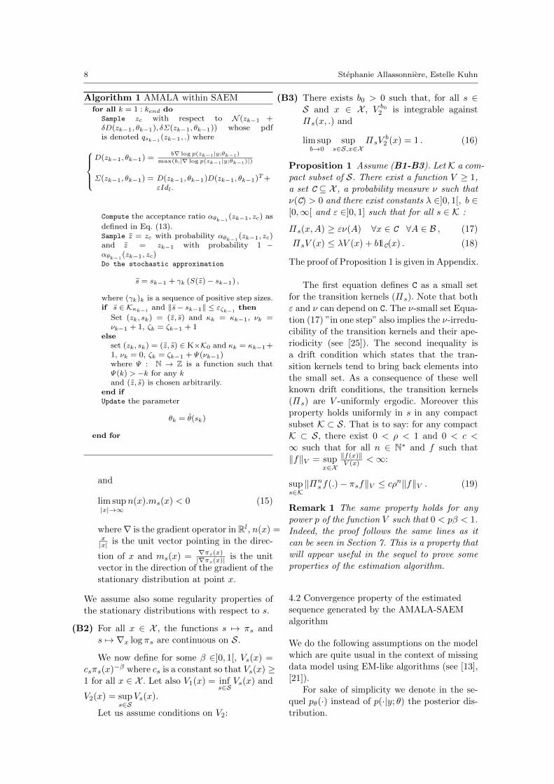
As a first experiment, we compare the mixing

properties of MALA and AMALA samplers.

We used both algorithms to sample from a 10

dimensional normal distribution with zero mean

and non diagonal covariance matrix. Its eigen-

values range from 1 to 10. The eigen-directions

are chosen randomly. The autocorrelations of

both chains are plotted in Fig. 1 where we can

see that there is a benefit of using the anisotropic

sampler. To evaluate the weight of the anisotropic

term D(x)D(x)T in the covariance matrix, we

compute its amplitude (as its non zero eigen-

value since it is a rank one matrix). We see that

it is of the same order as the diagonal part in

average and jumps up to 15 times bigger. This

shows the importance of the anisotropic term.

The last check is the Mean Square Euclidean

Jump Distance (MSEJD) which computes the

expected squared distance between successive

draws of the Markov chain. The two methods

provide MSEJD of the same order showing a

very slight advantage in term of visiting the

space for the AMALA sampler (1.29 versus 1.25

for the MALA).

We will observe in the following experiments

that the advantage of considering the AMALA

instead of the MALA sampler will be intensified

when increasing the problem dimension and in-

cluding it into our estimation process.

5.2 BME Template estimation

Back to our targeted application, we apply the

proposed estimation process on different data

bases. The first one is the USPS hand-written

digit base as used in [2] and [5]. The other two

are medical images of 2D corpus callosum and

3D murine dendrite spine excrescences used in

[4].

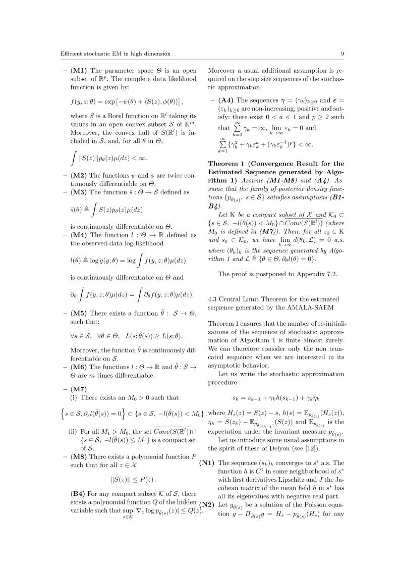
We begin with presenting the experiments

on the USPS database. In order to make com-parison, we estimate the parameters in the same

conditions as in the previous mentioned works

that is to say using the same 20 images per

digit. Each image has grey level between 0 (back-

ground) and 2 (bright white). These images

are presented on the top panel of Fig. 2. We

also use a noisy training dataset generated by

adding a standardized independent Gaussian

noise. These images are presented on the bot-

tom panel of Fig. 2. We test five algorithms: the

deterministic approximation of the EM algo-

rithm (FAM-EM) presented in [2], four MCMC-

SAEM where the sampler is either the MALA,

the adaptive MALA proposed in [7], the hy-

brid Gibbs sampler presented in [5] and our

AMALA algorithm.

For these experiments the tuning parame-

ters are chosen as follows: the threshold b is set

to 1, 000, the scale δ to 10−3 and the regular-

ization ε to 10−4. The other tuning parameters

and hyper-parameters are chosen as in [5].

Efficient stochastic EM in high dimension 11

Fig. 1 Autocorrelations of the MALA (blue) and AMALA (red) samplers to target the 10 dimensionalnormal distribution with anisotropic covariance matrix.

Fig. 2 Top: twenty images per digit of the trainingset used for the estimation of the model parameters(inverse video). Bottom: same images with additivenoise of variance 1.

Note that this model satisfies the conditions

of our convergence theorem as these conditions

are similar to the ones proved in [5].

5.3 Computational performances

We compare first the computational performances

of the algorithms. The computational time is

smaller for the three MCMC-SAEM algorithms

using ”MALA-like” samplers compared to the

FAM. Indeed, a numerical convergence of that

algorithm requires about 30 to 50 EM steps.

Each of them requires a gradient descent which

has 15 iterations in average. This implies to

compute 15 times the gradient of the energy

(which actually equals our gradient) for each

image for each EM step. The ”MALA-like”-

SAEM algorithms require about 100 to 150 EM

steps (depending on the digit) but only one gra-

dient is computed for each image at each step.

This reduces the computational time by a fac-

tor of at least 4 (up to 7 depending on the

digit). No comparison can be done when the

data are noisy since the FAM-EM does not con-

verges toward the MAP estimator as mentioned

above. Comparing to the hybrid Gibbs-SAEM,

the computational time is 8 times lower with

the AMALA-SAEM in this particular case of

application. Indeed, the hybrid Gibbs sampler

requires no computation of the gradient. How-

ever, it includes a loop over the coordinates of

the hidden variable, here the deformation vec-

tor of size 2kg = 72. At each of these itera-

tions, the candidate is straightforward to sam-

ple whereas the computational cost lies into the

acceptance rate. When this becomes heavy, the

less times you calculate it, the better. In the

AMALA-SAEM, this acceptance rate only has

to be calculated once for each image. There-

fore, even when the dimension of the hidden

variable increases, this is of constant cost. The

main price to pay is the computation of the

gradient. Therefore, a tradeoff has to be found

between the computation of either one gradi-

ent or dkg acceptance rates in order to select

the algorithm to use in a given case.

5.4 Results on the template estimation

All the estimated templates obtained with the

five algorithms and noise-free and noisy train-

ing data are presented in Fig. 3. As noticed

in [5], the FAM-EM estimation is sharp when

the training set is noise-free and is deteriorated

while adding noise. This behavior is not sur-

prising with regard to the theoretical bound

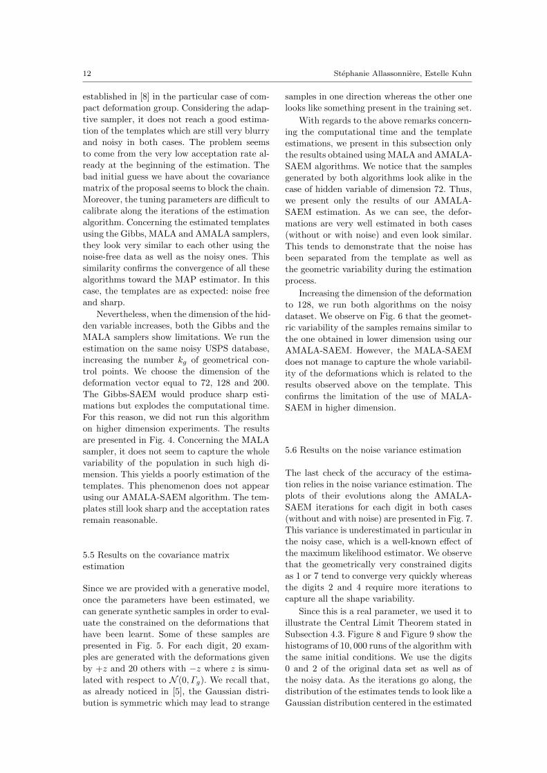
12 Stephanie Allassonniere, Estelle Kuhn

established in [8] in the particular case of com-

pact deformation group. Considering the adap-

tive sampler, it does not reach a good estima-

tion of the templates which are still very blurry

and noisy in both cases. The problem seems

to come from the very low acceptation rate al-

ready at the beginning of the estimation. The

bad initial guess we have about the covariance

matrix of the proposal seems to block the chain.

Moreover, the tuning parameters are difficult to

calibrate along the iterations of the estimation

algorithm. Concerning the estimated templates

using the Gibbs, MALA and AMALA samplers,

they look very similar to each other using the

noise-free data as well as the noisy ones. This

similarity confirms the convergence of all these

algorithms toward the MAP estimator. In this

case, the templates are as expected: noise free

and sharp.

Nevertheless, when the dimension of the hid-

den variable increases, both the Gibbs and the

MALA samplers show limitations. We run the

estimation on the same noisy USPS database,

increasing the number kg of geometrical con-

trol points. We choose the dimension of the

deformation vector equal to 72, 128 and 200.

The Gibbs-SAEM would produce sharp esti-

mations but explodes the computational time.

For this reason, we did not run this algorithm

on higher dimension experiments. The results

are presented in Fig. 4. Concerning the MALA

sampler, it does not seem to capture the whole

variability of the population in such high di-

mension. This yields a poorly estimation of the

templates. This phenomenon does not appear

using our AMALA-SAEM algorithm. The tem-

plates still look sharp and the acceptation rates

remain reasonable.

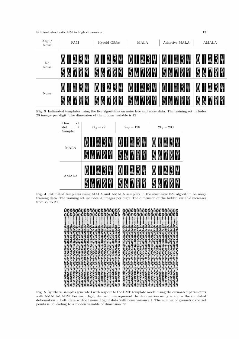
5.5 Results on the covariance matrix

estimation

Since we are provided with a generative model,

once the parameters have been estimated, we

can generate synthetic samples in order to eval-

uate the constrained on the deformations that

have been learnt. Some of these samples are

presented in Fig. 5. For each digit, 20 exam-

ples are generated with the deformations given

by +z and 20 others with −z where z is simu-

lated with respect to N (0, Γg). We recall that,

as already noticed in [5], the Gaussian distri-

bution is symmetric which may lead to strange

samples in one direction whereas the other one

looks like something present in the training set.

With regards to the above remarks concern-

ing the computational time and the template

estimations, we present in this subsection only

the results obtained using MALA and AMALA-

SAEM algorithms. We notice that the samples

generated by both algorithms look alike in the

case of hidden variable of dimension 72. Thus,

we present only the results of our AMALA-

SAEM estimation. As we can see, the defor-

mations are very well estimated in both cases

(without or with noise) and even look similar.

This tends to demonstrate that the noise has

been separated from the template as well as

the geometric variability during the estimation

process.

Increasing the dimension of the deformation

to 128, we run both algorithms on the noisy

dataset. We observe on Fig. 6 that the geomet-

ric variability of the samples remains similar to

the one obtained in lower dimension using our

AMALA-SAEM. However, the MALA-SAEM

does not manage to capture the whole variabil-

ity of the deformations which is related to the

results observed above on the template. This

confirms the limitation of the use of MALA-

SAEM in higher dimension.

5.6 Results on the noise variance estimation

The last check of the accuracy of the estima-

tion relies in the noise variance estimation. The

plots of their evolutions along the AMALA-

SAEM iterations for each digit in both cases

(without and with noise) are presented in Fig. 7.

This variance is underestimated in particular in

the noisy case, which is a well-known effect of

the maximum likelihood estimator. We observe

that the geometrically very constrained digits

as 1 or 7 tend to converge very quickly whereas

the digits 2 and 4 require more iterations to

capture all the shape variability.

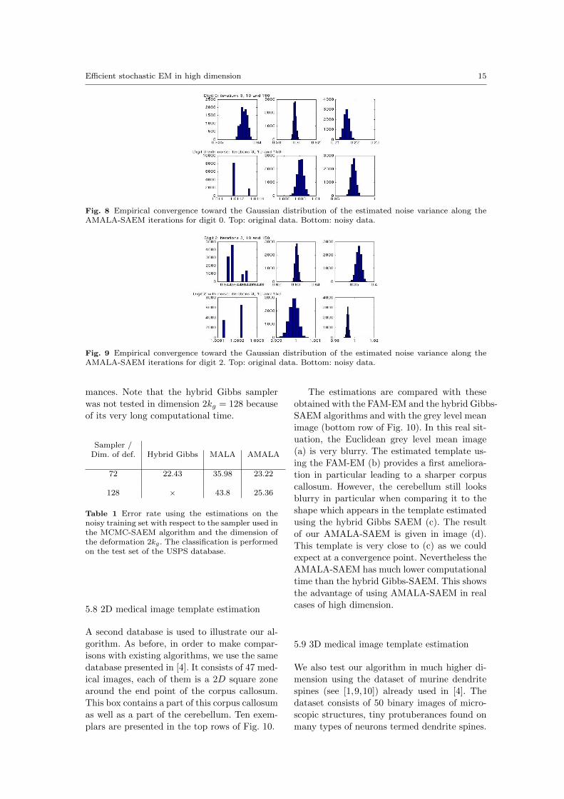
Since this is a real parameter, we used it to

illustrate the Central Limit Theorem stated in

Subsection 4.3. Figure 8 and Figure 9 show the

histograms of 10, 000 runs of the algorithm with

the same initial conditions. We use the digits

0 and 2 of the original data set as well as of

the noisy data. As the iterations go along, the

distribution of the estimates tends to look like a

Gaussian distribution centered in the estimated

Efficient stochastic EM in high dimension 13

Algo./Noise

FAM Hybrid Gibbs MALA Adaptive MALA AMALA

NoNoise

Noise

Fig. 3 Estimated templates using the five algorithms on noise free and noisy data. The training set includes20 images per digit. The dimension of the hidden variable is 72.

Dim. ofdef. /Sampler

2kg = 72 2kg = 128 2kg = 200

MALA

AMALA

Fig. 4 Estimated templates using MALA and AMALA samplers in the stochastic EM algorithm on noisytraining data. The training set includes 20 images per digit. The dimension of the hidden variable increasesfrom 72 to 200.

Fig. 5 Synthetic samples generated with respect to the BME template model using the estimated parameterswith AMALA-SAEM. For each digit, the two lines represent the deformation using + and − the simulateddeformation z. Left: data without noise. Right: data with noise variance 1. The number of geometric controlpoints is 36 leading to a hidden variable of dimension 72.

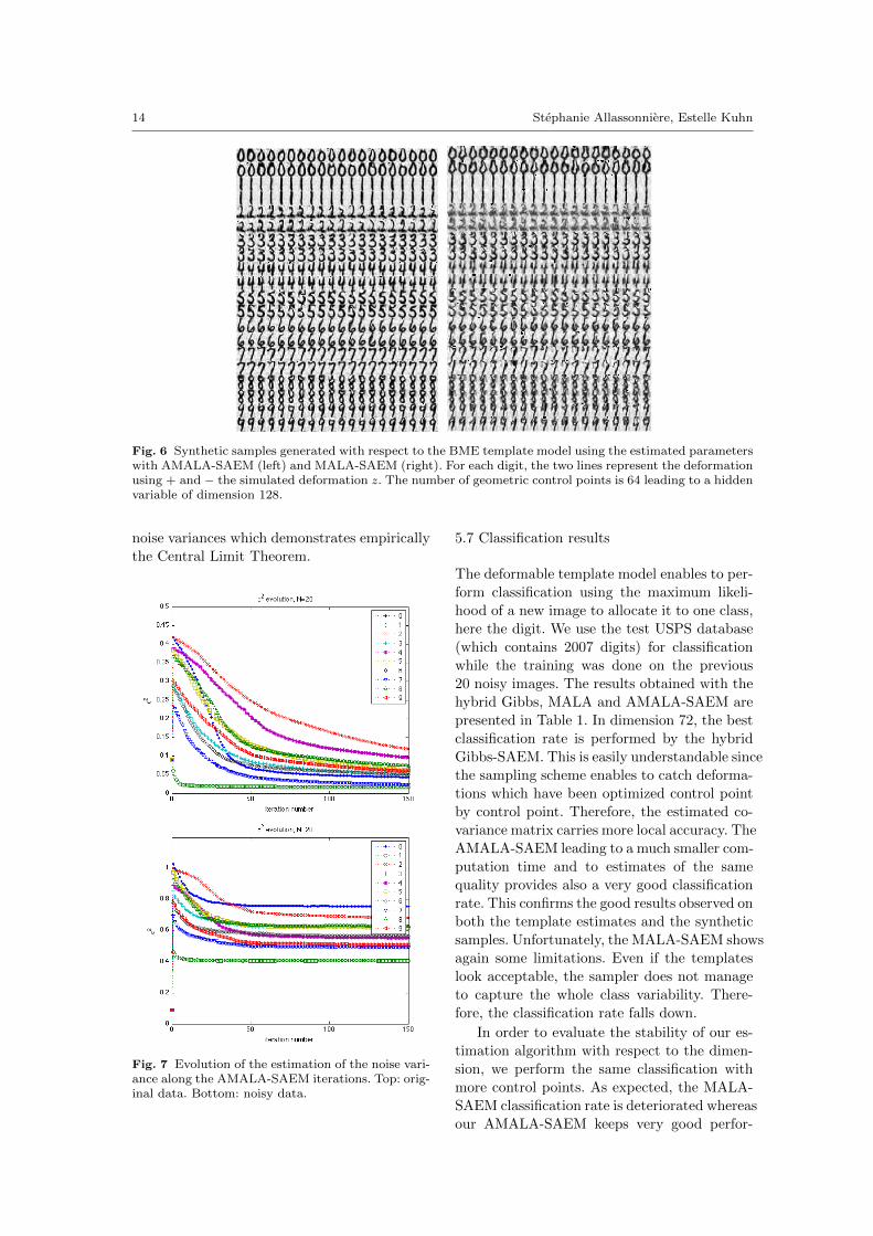
14 Stephanie Allassonniere, Estelle Kuhn

Fig. 6 Synthetic samples generated with respect to the BME template model using the estimated parameterswith AMALA-SAEM (left) and MALA-SAEM (right). For each digit, the two lines represent the deformationusing + and − the simulated deformation z. The number of geometric control points is 64 leading to a hiddenvariable of dimension 128.

noise variances which demonstrates empirically

the Central Limit Theorem.

Fig. 7 Evolution of the estimation of the noise vari-ance along the AMALA-SAEM iterations. Top: orig-inal data. Bottom: noisy data.

5.7 Classification results

The deformable template model enables to per-

form classification using the maximum likeli-

hood of a new image to allocate it to one class,

here the digit. We use the test USPS database

(which contains 2007 digits) for classification

while the training was done on the previous

20 noisy images. The results obtained with the

hybrid Gibbs, MALA and AMALA-SAEM are

presented in Table 1. In dimension 72, the best

classification rate is performed by the hybrid

Gibbs-SAEM. This is easily understandable since

the sampling scheme enables to catch deforma-

tions which have been optimized control point

by control point. Therefore, the estimated co-

variance matrix carries more local accuracy. The

AMALA-SAEM leading to a much smaller com-

putation time and to estimates of the same

quality provides also a very good classification

rate. This confirms the good results observed on

both the template estimates and the synthetic

samples. Unfortunately, the MALA-SAEM shows

again some limitations. Even if the templates

look acceptable, the sampler does not manage

to capture the whole class variability. There-

fore, the classification rate falls down.

In order to evaluate the stability of our es-timation algorithm with respect to the dimen-

sion, we perform the same classification with

more control points. As expected, the MALA-

SAEM classification rate is deteriorated whereas

our AMALA-SAEM keeps very good perfor-

Efficient stochastic EM in high dimension 15

Fig. 8 Empirical convergence toward the Gaussian distribution of the estimated noise variance along theAMALA-SAEM iterations for digit 0. Top: original data. Bottom: noisy data.

Fig. 9 Empirical convergence toward the Gaussian distribution of the estimated noise variance along theAMALA-SAEM iterations for digit 2. Top: original data. Bottom: noisy data.

mances. Note that the hybrid Gibbs sampler

was not tested in dimension 2kg = 128 because

of its very long computational time.

Sampler /Dim. of def. Hybrid Gibbs MALA AMALA

72 22.43 35.98 23.22

128 × 43.8 25.36

Table 1 Error rate using the estimations on thenoisy training set with respect to the sampler used inthe MCMC-SAEM algorithm and the dimension ofthe deformation 2kg. The classification is performedon the test set of the USPS database.

5.8 2D medical image template estimation

A second database is used to illustrate our al-

gorithm. As before, in order to make compar-

isons with existing algorithms, we use the same

database presented in [4]. It consists of 47 med-

ical images, each of them is a 2D square zone

around the end point of the corpus callosum.

This box contains a part of this corpus callosum

as well as a part of the cerebellum. Ten exem-

plars are presented in the top rows of Fig. 10.

The estimations are compared with these

obtained with the FAM-EM and the hybrid Gibbs-

SAEM algorithms and with the grey level mean

image (bottom row of Fig. 10). In this real sit-

uation, the Euclidean grey level mean image

(a) is very blurry. The estimated template us-

ing the FAM-EM (b) provides a first ameliora-

tion in particular leading to a sharper corpus

callosum. However, the cerebellum still looks

blurry in particular when comparing it to the

shape which appears in the template estimated

using the hybrid Gibbs SAEM (c). The result

of our AMALA-SAEM is given in image (d).

This template is very close to (c) as we could

expect at a convergence point. Nevertheless the

AMALA-SAEM has much lower computational

time than the hybrid Gibbs-SAEM. This shows

the advantage of using AMALA-SAEM in real

cases of high dimension.

5.9 3D medical image template estimation

We also test our algorithm in much higher di-

mension using the dataset of murine dendrite

spines (see [1,9,10]) already used in [4]. The

dataset consists of 50 binary images of micro-

scopic structures, tiny protuberances found on

many types of neurons termed dendrite spines.

16 Stephanie Allassonniere, Estelle Kuhn

(a) (b) (c) (d)

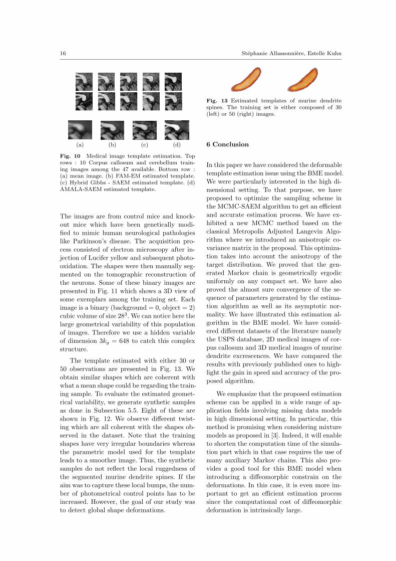
Fig. 10 Medical image template estimation. Toprows : 10 Corpus callosum and cerebellum train-ing images among the 47 available. Bottom row :(a) mean image. (b) FAM-EM estimated template.(c) Hybrid Gibbs - SAEM estimated template. (d)AMALA-SAEM estimated template.

The images are from control mice and knock-

out mice which have been genetically modi-

fied to mimic human neurological pathologies

like Parkinson’s disease. The acquisition pro-

cess consisted of electron microscopy after in-

jection of Lucifer yellow and subsequent photo-

oxidation. The shapes were then manually seg-

mented on the tomographic reconstruction of

the neurons. Some of these binary images are

presented in Fig. 11 which shows a 3D view of

some exemplars among the training set. Each

image is a binary (background = 0, object = 2)

cubic volume of size 283. We can notice here the

large geometrical variability of this population

of images. Therefore we use a hidden variableof dimension 3kg = 648 to catch this complex

structure.

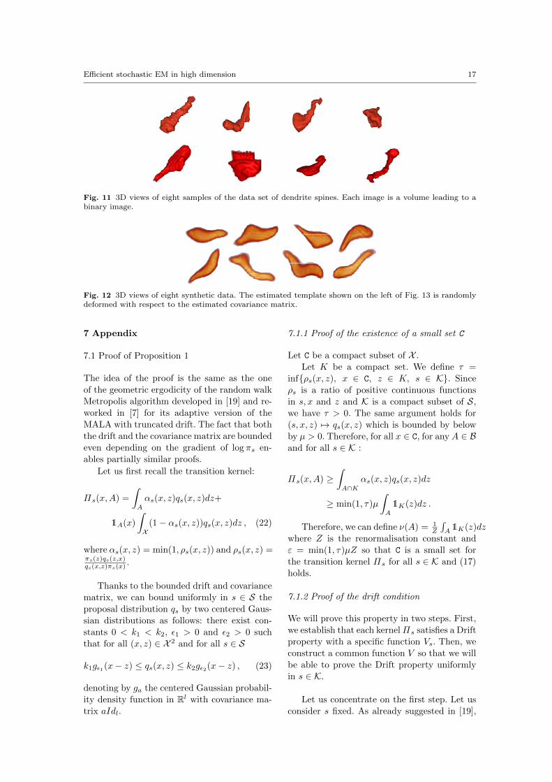
The template estimated with either 30 or

50 observations are presented in Fig. 13. We

obtain similar shapes which are coherent with

what a mean shape could be regarding the train-

ing sample. To evaluate the estimated geomet-

rical variability, we generate synthetic samples

as done in Subsection 5.5. Eight of these are

shown in Fig. 12. We observe different twist-

ing which are all coherent with the shapes ob-

served in the dataset. Note that the training

shapes have very irregular boundaries whereas

the parametric model used for the template

leads to a smoother image. Thus, the synthetic

samples do not reflect the local ruggedness of

the segmented murine dendrite spines. If the

aim was to capture these local bumps, the num-

ber of photometrical control points has to be

increased. However, the goal of our study was

to detect global shape deformations.

Fig. 13 Estimated templates of murine dendritespines. The training set is either composed of 30(left) or 50 (right) images.

6 Conclusion

In this paper we have considered the deformable

template estimation issue using the BME model.

We were particularly interested in the high di-

mensional setting. To that purpose, we have

proposed to optimize the sampling scheme in

the MCMC-SAEM algorithm to get an efficient

and accurate estimation process. We have ex-

hibited a new MCMC method based on the

classical Metropolis Adjusted Langevin Algo-

rithm where we introduced an anisotropic co-

variance matrix in the proposal. This optimiza-

tion takes into account the anisotropy of the

target distribution. We proved that the gen-

erated Markov chain is geometrically ergodic

uniformly on any compact set. We have also

proved the almost sure convergence of the se-

quence of parameters generated by the estima-

tion algorithm as well as its asymptotic nor-

mality. We have illustrated this estimation al-

gorithm in the BME model. We have consid-

ered different datasets of the literature namely

the USPS database, 2D medical images of cor-

pus callosum and 3D medical images of murine

dendrite excrescences. We have compared the

results with previously published ones to high-

light the gain in speed and accuracy of the pro-

posed algorithm.

We emphasize that the proposed estimation

scheme can be applied in a wide range of ap-

plication fields involving missing data models

in high dimensional setting. In particular, this

method is promising when considering mixture

models as proposed in [3]. Indeed, it will enable

to shorten the computation time of the simula-

tion part which in that case requires the use of

many auxiliary Markov chains. This also pro-

vides a good tool for this BME model when

introducing a diffeomorphic constrain on the

deformations. In this case, it is even more im-

portant to get an efficient estimation process

since the computational cost of diffeomorphic

deformation is intrinsically large.

Efficient stochastic EM in high dimension 17

Fig. 11 3D views of eight samples of the data set of dendrite spines. Each image is a volume leading to abinary image.

Fig. 12 3D views of eight synthetic data. The estimated template shown on the left of Fig. 13 is randomlydeformed with respect to the estimated covariance matrix.

7 Appendix

7.1 Proof of Proposition 1

The idea of the proof is the same as the one

of the geometric ergodicity of the random walk

Metropolis algorithm developed in [19] and re-

worked in [7] for its adaptive version of the

MALA with truncated drift. The fact that both

the drift and the covariance matrix are bounded

even depending on the gradient of log πs en-

ables partially similar proofs.

Let us first recall the transition kernel:

Πs(x,A) =

∫A

αs(x, z)qs(x, z)dz+

1A(x)

∫X

(1− αs(x, z))qs(x, z)dz , (22)

where αs(x, z) = min(1, ρs(x, z)) and ρs(x, z) =πs(z)qs(z,x)qs(x,z)πs(x)

.

Thanks to the bounded drift and covariance

matrix, we can bound uniformly in s ∈ S the

proposal distribution qs by two centered Gaus-

sian distributions as follows: there exist con-

stants 0 < k1 < k2, ε1 > 0 and ε2 > 0 such

that for all (x, z) ∈ X 2 and for all s ∈ S

k1gε1(x− z) ≤ qs(x, z) ≤ k2gε2(x− z) , (23)

denoting by ga the centered Gaussian probabil-

ity density function in Rl with covariance ma-

trix aIdl.

7.1.1 Proof of the existence of a small set C

Let C be a compact subset of X .

Let K be a compact set. We define τ =

inf{ρs(x, z), x ∈ C, z ∈ K, s ∈ K}. Since

ρs is a ratio of positive continuous functions

in s, x and z and K is a compact subset of S,

we have τ > 0. The same argument holds for

(s, x, z) 7→ qs(x, z) which is bounded by below

by µ > 0. Therefore, for all x ∈ C, for any A ∈ Band for all s ∈ K :

Πs(x,A) ≥∫A∩K

αs(x, z)qs(x, z)dz

≥ min(1, τ)µ

∫A

1K(z)dz .

Therefore, we can define ν(A) = 1Z

∫A1K(z)dz

where Z is the renormalisation constant and

ε = min(1, τ)µZ so that C is a small set for

the transition kernel Πs for all s ∈ K and (17)

holds.

7.1.2 Proof of the drift condition

We will prove this property in two steps. First,

we establish that each kernelΠs satisfies a Drift

property with a specific function Vs. Then, we

construct a common function V so that we will

be able to prove the Drift property uniformly

in s ∈ K.

Let us concentrate on the first step. Let us

consider s fixed. As already suggested in [19],

18 Stephanie Allassonniere, Estelle Kuhn

we only need to prove the two following condi-

tions:

supx∈X

ΠsVs(x)

Vs(x)<∞ (24)

and

lim sup|x|→∞

ΠsVs(x)

Vs(x)< 1 . (25)

We take the same path as in [7] applied to our

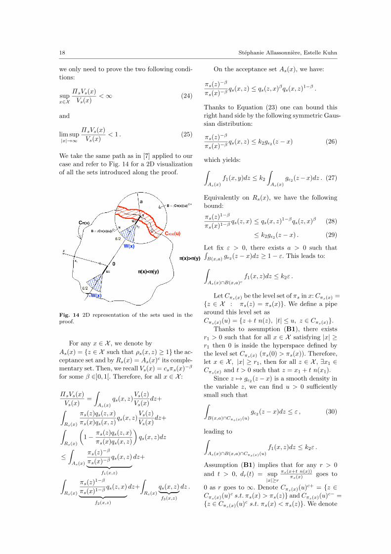
case and refer to Fig. 14 for a 2D visualization

of all the sets introduced along the proof.

Fig. 14 2D representation of the sets used in theproof.

For any x ∈ X , we denote by

As(x) = {z ∈ X such that ρs(x, z) ≥ 1} the ac-

ceptance set and by Rs(x) = As(x)c its comple-

mentary set. Then, we recall Vs(x) = csπs(x)−β

for some β ∈]0, 1[. Therefore, for all x ∈ X :

ΠsVs(x)

Vs(x)=

∫As(x)

qs(x, z)Vs(z)

Vs(x)dz+∫

Rs(x)

πs(z)qs(z, x)

πs(x)qs(x, z)qs(x, z)

Vs(z)

Vs(x)dz+∫

Rs(x)

(1− πs(z)qs(z, x)

πs(x)qs(x, z)

)qs(x, z)dz

≤∫As(x)

πs(z)−β

πs(x)−βqs(x, z)︸ ︷︷ ︸

f1(x,z)

dz+

∫Rs(x)

πs(z)1−β

πs(x)1−βqs(z, x)︸ ︷︷ ︸

f2(x,z)

dz+

∫Rs(x)

qs(x, z)︸ ︷︷ ︸f3(x,z)

dz .

On the acceptance set As(x), we have:

πs(z)−β

πs(x)−βqs(x, z) ≤ qs(z, x)βqs(x, z)

1−β .

Thanks to Equation (23) one can bound this

right hand side by the following symmetric Gaus-

sian distribution:

πs(z)−β

πs(x)−βqs(x, z) ≤ k2gε2(z − x) (26)

which yields:∫As(x)

f1(x, y)dz ≤ k2∫As(x)

gε2(z−x)dz . (27)

Equivalently on Rs(x), we have the following

bound:

πs(z)1−β

πs(x)1−βqs(z, x) ≤ qs(x, z)

1−βqs(z, x)β (28)

≤ k2gε2(z − x) . (29)

Let fix ε > 0, there exists a > 0 such that∫B(x,a)

gε2(z − x)dz ≥ 1− ε. This leads to:∫As(x)∩B(x,a)c

f1(x, z)dz ≤ k2ε .

Let Cπs(x) be the level set of πs in x: Cπs(x) =

{z ∈ X : πs(z) = πs(x)}. We define a pipe

around this level set as

Cπs(x)(u) = {z + t n(z), |t| ≤ u, z ∈ Cπs(x)}.Thanks to assumption (B1), there exists

r1 > 0 such that for all x ∈ X satisfying |x| ≥r1 then 0 is inside the hyperspace defined by

the level set Cπs(x) (πs(0) > πs(x)). Therefore,

let x ∈ X , |x| ≥ r1, then for all z ∈ X , ∃x1 ∈Cπs(x) and t > 0 such that z = x1 + t n(x1).

Since z 7→ gε2(z − x) is a smooth density in

the variable z, we can find u > 0 sufficiently

small such that∫B(x,a)∩Cπs(x)(u)

gε2(z − x)dz ≤ ε , (30)

leading to∫As(x)∩B(x,a)∩Cπs(x)(u)

f1(x, z)dz ≤ k2ε .

Assumption (B1) implies that for any r > 0

and t > 0, dr(t) = sup|x|≥r

πs(x+t n(x))πs(x)

goes to

0 as r goes to ∞. Denote Cπs(x)(u)c+ = {z ∈Cπs(x)(u)c s.t. πs(x) > πs(z)} and Cπs(x)(u)c− =

{z ∈ Cπs(x)(u)c s.t. πs(x) < πs(z)}. We denote

Efficient stochastic EM in high dimension 19

D+ = As(x) ∩ B(x, a) ∩ Cπs(x)(u)c+. There-

fore there exists r2 > r1 + a such that for any

x, |x| ≥ r2∫D+

f1(x, z)dz ≤∫D+

(πs(z)

πs(x)

)1−β

qs(z, x)dz

≤ dr2(u)1−βk2

∫Xgε2(z − x)dz

≤ k2dr2(u)1−β ,

using Equation (15) which states that the sta-

tionary distribution is decreasing in the direc-

tion of the normal of x sufficiently large.

In the same way, one has on the set D− =

As(x) ∩B(x, a) ∩ Cπs(x)(u)c−∫D−

f1(x, z)dz ≤∫D−

(πs(z)

πs(x)

)−βqs(x, z)dz

≤ k2dr2(u)β .

The same inequalities can be obtained for f2using the same arguments:∫

Rs(x)∩B(x,a)cf2(x, z)dz ≤ k2ε∫

Rs(x)∩B(x,a)∩Cπs(x)(u)f2(x, z)dz ≤ k2ε∫

Rs(x)∩B(x,a)∩Cπs(x)(u)c+f2(x, z)dz ≤ k2dr2(u)1−β∫

Rs(x)∩B(x,a)∩Cπs(x)(u)c−f2(x, z)dz ≤ k2dr2(u)β .

This yields

lim sup|x|→∞

ΠsVs(x)

Vs(x)≤ lim sup|x|→∞

∫Rs(x)

qs(x, z)dz.

(31)

Let Q(x,As(x)) =∫As(x)

qs(x, z)dz, we get

lim sup|x|→∞

ΠsVs(x)

Vs(x)≤ 1− lim inf

|x|→∞Q(x,As(x)).

Let us now prove that

lim inf|x|→∞

Q(x,As(x)) ≥ c > 0 where c does not

depend on x.

Let a fixed as above. Since qs is an expo-

nential function, there exists ca0 > 0 such that

for all x ∈ X and s ∈ S,

infz∈B(x,a)

qs(z, x)

qs(x, z)≥ ca0 . (32)

Moreover, thanks to assumption (B1) there ex-

ists r3 > 0 such that for all x ∈ X , |x| ≥ r3,

there exists 0 < u2 < a such that,

πs(x)

πs(x− u2 n(x))≤ ca0 . (33)

Hence, for |x| ≥ r3, any point x2 = x−u2 n(x)

belongs to As(x).

Let W (x) be the cone defined as:

W (x) ={x2 − tζ, 0 < t < a− u2, ζ ∈ Sd−1,

|ζ − n(x2)| ≤ ε

2

}(34)

where Sd−1 is the unit sphere in Rd.

Let us prove that W (x) ⊂ As(x).

Using assumption (B1), we have for a suf-

ficiently large x: m(x).n(x) ≤ −ε. Besides, by

construction of W (x) for large x, for all z ∈W (x), |n(z) − n(x)| ≤ ε/2 with n(x) = n(x2)

(see Fig. 14). This leads to for any sufficiently

large x, for all z ∈W (x),

m(z).ζ = m(z).(ζ−n(x2))+m(z).(n(x2)−n(z))

+m(z).n(z) ≤ ε/2 + ε/2− ε = 0 . (35)

Let now z = x2 − tζ ∈ W (x). Using the mean

value theorem on the differentiable function πsbetween x2 and z, we get that there exists τ ∈]0, s[ such that πs(z) − π(x2) = −tζ.∇πs(x2 −τζ). Using the definition of m, this implies that

πs(z) − πs(x2) = −tζ.m(x2 − τζ)|∇πs(x2 −τζ)| ≥ 0 thanks to Equation (35). Putting all

these results together we finally get that for all

z ∈ W (x), πs(z) ≥ πs(x2) ≥ 1ca0πs(x). More-

over, as z ∈ B(x, a) as well, Equation (32) is

satisfied, leading to z ∈ As(x).

Then, we have

Q(x,As(x)) =

∫As(x)

qs(x, z)dz

≥∫As(x)

k1gε1(z − x)dz

≥ k1

∫W (x)

gε1(z − x)dz

=

∫Tx(W (x))

gε1(z)dz

where

Tx(W (x)) ={−u2 n(x)− tζ, 0 < t < a− u2,

ζ ∈ Sd−1, |ζ − n(x)| ≤ ε

2

}(36)

is the translation of the set W (x) by the vec-

tor x. Note that W (x) does not depend on s.

But since gε1 is isotropic and Tx(W (x)) only

depends on a fixed constant u2 and n(x), this

last integral is independent of x, so there exists

20 Stephanie Allassonniere, Estelle Kuhn

a positive constant c independent of s ∈ S such

that:

c =

∫Tx(W (x))

gε1(z)dz . (37)

Back to our limit, for all s ∈ S

lim sup|x|→∞

ΠsVs(x)

Vs(x)≤ 1− c (38)

which ends the proof of the condition (25).

To prove (24), we use the previous result.

Indeed, since ΠsVs(x)Vs(x)

is a smooth function on Xit is bounded on every compact subset. More-

over since the lim sup is finite, then it is also

bounded outside a fixed compact. This proves

the results.

Thanks to assumption (B2) and the bounded

drift for all s ∈ S, there exists a constant ca0uniform in s ∈ S such that Equations (32)

and (33) still hold for all s ∈ S. This implies,

as mentioned above, that the set Tx(W (x)) is

independent of s ∈ S. Therefore, we can set

λ = 1 − c < 1 where c is defined in Equation

(37) and is also independent of s ∈ S.

This proves the Drift property for the func-

tion Vs: there exist constants 0 < λ < 1 and

b > 0 such that for all x ∈ X ,

ΠsVs(x) ≤ λVs(x) + b1C(x) , (39)

where C is a small set. Note that b is also inde-pendent of s ∈ S using the same arguments as

before.

Let us now exhibit a function V indepen-

dent of s ∈ S and prove the uniform Drift con-

dition.

We define for all x ∈ X ,

V (x) = V1(x)ξV2(x)2ξ (40)

for 0 < ξ < min(1/2β, b0/4). Therefore, for all

s ∈ S, for all ε > 0 we have,

ΠsV (x) =

∫XΠs(x, z)V1(z)ξV2(z)2ξdz

≤ 1

2

∫XΠs(x, z)

(V1(z)2ξ

ε2+ ε2V2(z)4ξ

)dz

≤ 1

2ε2

∫XΠs(x, z)Vs(z)

2ξdz+

ε2

2

∫XΠs(x, z)V2(z)4ξdz . (41)

Applying the Drift property for Πs with V 2ξs ,

ΠsV (x) ≤ 1

2ε2(λVs(x)2ξ + b1C(x))

+ε2

2

∫XΠs(x, z)V2(z)4ξdz . (42)

Using the definition of V and the fact that V1is bounded by below by 1, we get:

ΠsV (x) ≤ λ

2ε2V (x) +

b

2ε21C(x)

+ε2

2

∫XΠs(x, z)V2(z)4ξdz . (43)

Since 0 < λ < 1 is independent of s ∈ Sand using assumption (B3), there exists ξ > 0

such that

sups∈S,x∈X

∫XΠs(x, z)V2(z)4ξdz ≤ 2

1 + λ. (44)

This yields

ΠsV (x) ≤

(λ

2ε2+

ε2

1 + λ

)V (x)+

b

2ε21C(x) .

(45)

We can now fix ε2 =

√λ(1+λ)

2 which leads to

ΠsV (x) ≤

√2λ

1 + λV (x) +

b

2ε21C(x) . (46)

We set λ =√

2λ1+λ

< 1 and b = b2ε2 > 0

which concludes the proof.

7.2 Proof of Theorem 1

We provide here the proof of the convergence of

the estimated sequence generated by Algorithm

1.

We apply Theorem 4.1 from [5] with the

functions Hs equals to Hs(z) = S(z)− s, Πs =

Π θ(s), πs = pθ(s) and

h(s) =

∫(S(z)− s)pθ(s)(z)µ(dz) .

Let us first prove assumption (A1’) which

ensures the existence of a global Lyapunov func-

tion for the mean field of the stochastic approx-

imation. It guaranties that, under some condi-

tions, the sequence (sk)k≥0 remains in a com-

pact subset of S and converges to the set of

critical points of the log-likelihood.

Efficient stochastic EM in high dimension 21

Assumptions (M1)-(M7) ensure that S is

an open subset and that the function h is con-

tinuous on S. Moreover defining w(s) = −l(θ(s)),we get that w is continuously differentiable on

S. Applying Lemma 2 of [13], we get (A1’)(i),

(A1’)(iii) and (A1’)(iv).

To prove (A1’)(ii), we consider as absorb-

ing set Sa the closure of the convex hull of S(Rl)denoted Conv(S(Rl)). So assumption (M7)(ii)

is exactly equivalent to assumption (A1’)(ii).

This achieves the proof of assumption (A1’).

Let us now prove assumption (A2) which

states in particular the existence of a unique

invariant distribution for the Markov chain.

To that purpose, we prove that our family of

kernels satisfies the drift conditions mentioned

in [6] and used in [5] in a similar context. These

conditions are the existence of a small set uni-

formly in s ∈ K, the uniform drift condition

and an upper bound on the family kernel :

(DRI1) For any s ∈ S, Π θ(s) is ψ-irreducible and

aperiodic. In addition there exist a function

V : Rl → [1,∞[ and a constant p ≥ 2 such

that for any compact subset K ⊂ S, there

exist an integer j and constants 0 < λ < 1,

B, κ, δ > 0 and a probability measure ν

such that

sups∈K

Πj

θ(s)V p(z) ≤ λV p(z) +B1C(z) , (47)

sups∈K

Π θ(s)Vp(z) ≤ κV p(z) ∀z ∈ X , (48)

infs∈K

Πj

θ(s)(z,A) ≥ δν(A) ∀z ∈ C,∀A ∈ B .(49)

Let us start with the irreducibility of Π θ(s).

The kernel Π θ(s) is bounded by below as fol-

lows :

Π θ(s)(x,A) ≥∫A

αs(x, z)qs(x, z)dz , (50)

where αs(x, z) = min(1, ρs(x, z)) and ρs(x, z) =πs(z)qs(z,x)qs(x,z)πs(x)

> 0. Since the proposal density qsis positive, this proves that Πs(x,A) is posi-

tive and the ψ-irreducibility of each kernel of

the family.

Proposition 1 and Remark 1 show that Equa-

tions (47) and (49) hold for j = 1 with V de-

fined in Equation (40) and some p > 2. More-

over, since Equation (47) holds for j = 1 and

V ≥ 1, Equation (48) directly comes from Equa-

tion (47) choosing κ = B + λ. This implies all

three inequalities. Since the small set condition

is satisfied with j = 1 (small set ”in one-step”),

each chain of the family is aperiodic (see [25]).

Assumption (A2) is therefore directly im-

plied by assumption (M1).

Let us now prove assumption (A3’) which

states some regularity conditions (Holder type

ones) on the solution of the Poisson equation

related to the transition kernel. It also ensures

that this solution and its image through the

transition kernel have reasonable behaviors as

the chain goes to infinity and that the kernel is

V p-bounded in expectation.

The drift conditions proved previously im-

ply the geometric ergodicity uniformly in s in

any compact set K. This also ensures the exis-

tence of a solution of the Poisson equation (see

[25]) required in Assumption (A3’).

We first consider condition (A3’(i)).

Let us define for any g : X → Rm the norm

‖g‖V , supz∈X

‖g(z)‖V (z) .

Since Hs(z) = S(z)−s, assumptions (M8) and

(B1) ensure that sups∈K‖Hs‖V <∞ and inequal-

ity (4.3) of (A3’(i)) holds.

The uniform ergodicity of the family of Markov

chains corresponding to the AMALA on K en-

sures that there exist constants 0 < γK < 1 and

CK > 0 such that for all s ∈ K

sups∈K‖gθ(s)‖V = sup

s∈K‖∑k≥0

(Πkθ(s)

Hs − pθ(s)Hs)‖V

≤ sups∈K

∑k≥0

CKγkK‖Hs‖V <∞ .

Thus for all s in K , gθ(s) belongs to LV = {g :

Rl → Rm, ‖g‖V <∞}.Repeating the same calculation as above, it

is immediate that sups∈K|‖Π θ(s)gθ(s)‖V is bounded.

This ends the proof of inequality (4.4) of (A3’(i)).

We now move to the Holder conditions (4.5)

of (A3’(i)). We will use the two following lem-

mas which state Holder conditions on the tran-

sition kernel and its iterates:

Lemma 1 Let K be a compact subset of S.

There exists a constant CK such that for all

1 ≤ p there exists q > p, for all function f ∈LV p and for all (s, s′) ∈ K2 we have :

‖Π θ(s)f −Π θ(s′)f‖V q ≤ CK‖f‖V p ‖s− s′‖ .

22 Stephanie Allassonniere, Estelle Kuhn

Proof For any f ∈ LV p and any x ∈ Rl, we

have

Πsf(x) =

∫Rlf(z)αs(x, z)qs(x, z)dz

+ f(x)(1 − αs(x)) ,

where αs(x, z) = min(

1,pθ(s)(z)qs(z,x)

qs(x,z)pθ(s)(x)

)and

αs(x) =∫αs(x, z)qs(x, z)dz is the average ac-

ceptance rate. Let us denote for all x, z and s:

rs(x, z) = αs(x, z)qs(x, z).

Let s and s′ be two points in K. We note

that s 7→ θ(s) is a continuously differentiable

function therefore uniformly bounded in s ∈ K.

‖Πsf(x)−Πs′f(x)‖ ≤ ‖f‖V p×{∫X|rs(x, z)− rs′(x, z)|V p(z)dz +

V p(x)

∫X|rs(x, z)− rs′(x, z)|dz

},

≤ 2‖f‖V pV p(x)×∫X|rs(x, z)− rs′(x, z)|V p(z)dz .

Let I =∫X |rs(x, z)− rs′(x, z)|V

p(z)dz. For

sake of simplicity, we denote by As the accep-

tance set instead of As(x). We decompose I

into four terms :

I =∫As∩As′

|rs(x, z)− rs′(x, z)|V p(z)dz(51)

+∫As∩Acs′

|rs(x, z)− rs′(x, z)|V p(z)dz

(52)

+∫Acs∩As′

|rs(x, z)− rs′(x, z)|V p(z)dz(53)

+∫Acs∩Acs′

|rs(x, z)− rs′(x, z)|V p(z)dz

. (54)

Let us first consider the term (51).∫As∩As′

|rs(x, z)− rs′(x, z)|V p(z)dz

=

∫As∩As′

|qs(x, z)− qs′(x, z)|V p(z)dz . (55)

We use the mean value theorem on the smooth

function s 7→ qs(x, z) for fixed values of (x, z).

dqs(x, z)

ds= qs(x, z)

d log qs(x, z)

ds.

After some calculations, using the bounded drift

and covariance and Assumption (M8), we get :

d log qs(x, z)

ds≤ P1(x, z)

(∥∥∥∥dDs(x)

ds

∥∥∥∥+

∥∥∥∥dΣs(x)

ds

∥∥∥∥F

+

∥∥∥∥dΣ−1s (x)

ds

∥∥∥∥F

),

≤ CKP1(x, z) .

where Ds and Σs are respectively the drift and

covariance of the proposal qs and P1 and P1 are

two polynomial functions in both variables.

Using Equation (23), we have :∣∣∣∣dqs(x, z)ds

∣∣∣∣ ≤ k2CKP1(x, z)gε2(z − x) ,

which leads to :∫As∩As′

|qs(x, z)− qs′(x, z)|V p(z)dz

≤ k2CK‖s− s′‖∫XV p(z)P1(x, z)gε2(z − x)dz

≤ k2CKQ1(x)‖s− s′‖ ,

where Q1 is a polynomial function.

Now we move to the second term (52). Let

z ∈ As ∩ Acs′ . We define for all u ∈ [0, 1] the

barycenter s(u) of s and s′ equals to us+ (1−u)s′ which belongs to the convex hull of the

compact subset K.

Since u 7→ ρs(u)(x, z) is continuously dif-

ferentiable, ρs(x, z) ≥ 1 and ρs′(x, z) < 1, us-

ing the intermediate value theorem, there ex-

ists u ∈]0, 1] depending on x and z such that

ρs(u)(x, z) = 1. We choose the minimum value

of u satisfying this condition. Therefore,

|αs(x, z)qs(x, z)− αs′(x, z)qs′(x, z)|≤ |qs(x, z)− qs(u)(x, z)|+|ρs(u)(x, z)qs(u)(x, z)− ρs′(x, z)qs′(x, z)| .

(56)

We treat the first term of the right hand

side as previously. For the second term, we use

the mean value theorem for the function v 7→fs(v)(x, z) = ρs(v)(x, z)qs(v)(x, z) on ]0, u[. There

exists v ∈]0, u[ such that

|fs(u)(x, z)− fs′(x, z)| ≤∣∣∣∣dfs(v)(x, z)dv

∣∣∣∣ ‖s− s′‖ .Thanks to the upper bound above we get

d log fs(v)(x, z)

dv≤ CKP2(x, z) ,

Efficient stochastic EM in high dimension 23

where P2 is a polynomial function in both vari-

ables. Since on the segment defined by s(u) and

s′ we have ρs(x, z) ≤ 1 :

dfs(v)(x, z)

dv= fs(v)(x, z)

d log fs(v)(x, z)

dv≤ CKqs(v)(x, z)P2(x, z)

≤ k2CK‖s− s′‖P2(x, z)gε2(z − x) .

This yields :∫As∩Acs′

|rs(x, z)− rs′(x, z)|V p(z)dz

≤ k2CK

(Q1(x) +Q2(x)

)‖s− s′‖ .

The third term (53) is the symmetric one of

the second.

Let us end with the last term (54).∫Acs∩Acs′

|αs(x, z)qs(x, z)− αs′(x, z)qs′(x, z)| ×

V p(z)dz

=

∫Acs∩Acs′

|ρs(x, z)qs(x, z)− ρs′(x, z)qs′(x, z)| ×

V p(z)dz .

If for all u ∈]0, 1[, ρs(u)(x, y) < 1 then this term

can be treated as the second term of Equa-

tion (56). If there exists u ∈]0, 1[ such that

ρs(u)(x, y) ≥ 1, we define u0 and u1 respec-

tively the smallest and biggest elements in ]0, 1[

such that ρs(u0) = ρs(u1) = 1. The first and last

terms are treated as the previous case and the

middle term is treated as the term (51).

Putting all these upper bounds together yields :

‖Πsf(x)−Πs′f(x)‖ ≤ 2‖f‖V pV p(x)Q(x)‖s−s′‖ ,(57)

where Q is a polynomial function in x ∈ X .

Therefore, there exists a constant q > p such

that V p(x)Q(x) ≤ V q(x) which concludes the

proof.

Lemma 2 Let K be a compact subset of S.

There exists a constant CK such that for all

1 ≤ p < q, for all function f ∈ LV p , for all

(s, s′) ∈ K2 and for all k ≥ 0, we have:

‖Πkθ(s)

f −Πkθ(s′)

f‖V q ≤ CK‖f‖V p‖s− s′‖ .

Proof The proof of lemma 2 follows the line of

the proof of Proposition B.2 of [6].

Thanks to the proofs of [5], we get that h

is a Holder function for any 0 < a < 1 which

leads to (A3”(i)).

We finally focus on the proof of (A3”(ii)).

Lemma 3 Let K be a compact subset of S and

p ≥ 1. For all sequences γ = (γk)k≥0 and ε =

(εk)k≥0 satisfying εk < ε for some ε sufficiently

small, there exists CK > 0, such that for any

z0 ∈ X , we have

sups∈K

supk≥0

Eγz,s[V p(zk)1σ(K)∧ν(ε)≥k] ≤ CKV p(z0) ,

where Eγz,s is the expectation related to the non-

homogeneous Markov chain ((zk, sk)) started from

(z, s) with step size sequence γ.

Proof Let K be a compact subset of Θ such

that θ(K) ⊂ K. We note in the sequel, θk =

θ(sk). We have for k ≥ 2, using the Markov

property and the drift property (18) for V p,

Eγz,s[V p(zk)1σ(K)∧ν(ε)≥k] ≤ Eγz,s[Πθk−1V p(zk−1)]

(58)

≤ λEγz,s[V p(zk−1)] + C .

(59)

Iterating the same arguments recursively leads

to :

Eγz,s[V p(zk)1σ(K)∧ν(ε)≥k]

≤ λkEγz,s[V p(z0)] + C

k−1∑l=0

λl .

Since λ < 1 and V (z) ≥ 1 for all z ∈ X , for

all k ∈ N, we have :

Eγz,s[V p(zk)1σ(K)∧ν(ε)≥k] ≤ V p(z0) + C

k−1∑l=0

λl

≤ V p(z0)

(1 +

C

1− λ

).

This yields (A3’(ii)) which concludes the

proof of Theorem 1.

24 Stephanie Allassonniere, Estelle Kuhn

7.3 Proof of the Central Limit Theorem for

the Estimated Sequence

The proof of Theorem 2 follows the lines of the

proof of Theorem 25 of [12]. This theorem is an

application of Theorem 24 of [12] in the case of

Markovian dynamics. However, some assump-

tions required in Theorem 24 are not fulfilled in

our case: the A-stability of the algorithm and

the boundedness in infinite norm of the solution

of the Poisson equation.

Consider the stochastic approximation:

sk = sk−1 + γkh(sk−1) + γkηk , (60)

where the remainder term is decomposed as fol-

lows:

ηk = ξk + νk − νk−1 + rk (61)

with

ξk = gθ(sk−1)(zk)−Π θ(sk−1)

gθ(sk−1)(zk−1)

(62)

νk = −Π θ(sk)gθ(sk)(zk) (63)

rk = Π θ(sk)gθ(sk)(zk)−Π θ(sk−1)

gθ(sk−1)(zk)

(64)

and for any s ∈ S, gθ(s) is a solution of the

Poisson equation g −Π θ(s)g = Hs − pθ(s)(Hs).

We recall Theorem 24 of [12] with sufficient

assumptions for our setting.

Theorem 3 (Adapted from Theorem 24

[12]) Let assumptions (N1) and (N3) be ful-

filled. Furthermore, assume that for some ma-

trix U , some ε > 0 and some positive random

variables X,X ′, X ′′:

The sequence (ξi) is a F −martingale (65)

supi∈N‖ξi‖2+ε <∞ (66)

limk→∞

γ−1/2k ‖Xrk‖1 = 0 (67)

limk→∞

γ1/2k ‖X

′νk‖1 = 0 (68)

limk→∞

γk‖X ′′k∑i=1

(ξiξTi − U)‖1 = 0 (69)

where F = (Fi)i∈N is the increasing family of

σ−algebra generated by the random variables

(s0, z1, ..., zi). Then

sk − s∗√γk

→L N (0, V ) (70)

where V is the solution of the following Lya-

punov equation U + JV + V JT = 0.

The result of Theorem 24 still holds replac-

ing assumption (C) of [12] by (N1). Indeed, it

is sufficient to establish that the random vari-

able γ−1/2k

k∑i=0

exp[(tk − ti)J ]γiri converges to-

ward 0 in probability where ti =i∑

j=1

γj . The-

orem 19 and Proposition 39 of [12] can be ap-

plied in expectation. Theorems 23 and 20 of

[12] also still hold with assumption (N1).

We now prove that assumptions of Theorem

3 hold.

By definition of ξi it is obvious that (65) is

fulfilled. Moreover, the following lemma proves

that there exists ε > 0 such that (66) holds

with X = 1.

Lemma 4 For all ε > 0, the sequence (ξk) is

in L2+ε.

Proof We use the convexity of the function x 7→x2+ε. Indeed, we have

|gθ(sk−1)(zk)−Π θ(sk−1)

gθ(sk−1)(zk−1)|2+ε

≤ (|gθ(sk−1)(zk)|+ |Π θ(sk−1)

gθ(sk−1)(zk−1)|)2+ε

≤ Cε(|gθ(sk−1)(zk)|2+ε+|Π θ(sk−1)

gθ(sk−1)(zk−1)|2+ε) ,

where Cε = 123+ε .

Applying the drift condition, we get :

E(||ξk||2+ε|Fk−1) ≤ Cε(E(|gθ(sk−1)

(zk)|2+ε | Fk−1)

+|E(Π θ(sk−1)gθ(sk−1)

(zk−1)|Fk−1)|2+ε)

≤ C E(V (zk)2+ε + V (zk−1)2+ε|Fk−1))

≤ C(λV 2+ε(zk−1) + 1

).

Finally taking the expectation after induction

as in Lemma 3 leads to:

E(||ξ2+εk ||) ≤ CV 2+ε(z0) < +∞ .

Let us now focus on Equation (67). Thanks

to the Holder property of our kernel and the

fact that Hsk belongs to LV :

‖rk‖1 = E[|Π θ(sk)gθ(sk)(zk)−Π θ(sk−1)

gθ(sk−1)(zk)|]

≤ CE[V q(zk)|sk − sk−1|a]

≤ CE[V q+1(zk)]γak

≤ Cγak

where the last inequality comes from the drift

property. Since the Holder property is true for

Efficient stochastic EM in high dimension 25

any 0 < a < 1, we can choose a > 1/2 which

leads to the conclusion.

To prove Equation (68), we note that using

the drift condition as in the previous lemma,

E(‖νk‖) is uniformly bounded in k. Since the

step-size sequence (γk)k tends to zero, the re-

sult follows with X ′ = 1.

We follow the lines of the proof of Theorem

25 of [12] to establish Equation (69). As in the

proof of Lemma 4, we use the drift property

coupled with our Holder condition in LV -norm

instead of the usual Holder condition consid-

ered by [12] which is denoted (MS).

This concludes the proof of Theorem 3.

Applying Theorem 3 allows to prove the

first part of Theorem 2. Assumption (N2) en-

ables to characterize the covariance matrix Γ .

The Delta method gives the result on the se-

quence (θk) achieving the proof of our Central

Limit Theorem.

References

1. Aldridge, G., Ratnanather, J., Martone, M.,Terada, M., Beg, M., Fong, L., Ceyhan, E., Ko-lasny, A., Brown, T., Cochran, E., Tang, S.,Pisano, D., Vaillant, M., Hurdal, M., Churchill,J., Greenough, W., Miller, M., Ellisman, M.:Semi-automated shape analysis of dendritespines from animal models of fragilex andparkinson’s disease using large deformation dif-feomorphic metric mapping. Society for Neuro-science Annual Meeting, Washington DC (2005)

2. Allassonniere, S., Amit, Y., Trouve, A.: Towarda coherent statistical framework for dense de-formable template estimation. JRSS 69, 3–29(2007)

3. Allassonniere, S., Kuhn, E.: Stochastic algo-rithm for bayesian mixture effect template esti-mation. ESAIM Probab Stat 14, 382–408 (2010)

4. Allassonniere, S., Kuhn, E., Trouve, A.:Bayesian consistent estimation in deformablemodels using stochastic algorithms: Applica-tions to medical images. Journal de la SocieteFrancaise de Statistique 151(1), 1–16 (2010)

5. Allassonniere, S., Kuhn, E., Trouve, A.:Bayesian deformable models building viastochastic approximation algorithm: A conver-gence study. Bernoulli J. 16(3), 641–678 (2010)

6. Andrieu, C., Moulines, E., Priouret, P.: Stabil-ity of stochastic approximation under verifiableconditions. SIAM J. Control Optim. 44(1), 283–312 (electronic) (2005)

7. Atchade, Y.: An adaptive version for themetropolis adjusted langevin algorithm with

a truncated drift. Methodol. Comput. Appl.Probab. 8, 235–254 (2006)

8. Bigot, J., Charlier, B.: On the consistency ofFrechet means in deformable models for curveand image analysis. Electron. J. Stat. 5, 1054–1089 (2011). DOI 10.1214/11-EJS633. URLhttp://dx.doi.org/10.1214/11-EJS633

9. Ceyhan, E., Fong, L., Tasky, T., Hurdal, M., BegM.F.and Martone, M., Ratnanather, J.: Type-specific analysis of morphometry of dendritespines of mice. 5th Int. Symp. Image SignalProc. Analysis, ISPA pp. 7–12 (2007)

10. Ceyhan, E., Olken, R., Fong, L., Tasky, T.,Hurdal, M., Beg, M., Martone, M., Rat-nanather, J.: Modeling metric distances of den-drite spines of mice based on morphometricmeasures. Int. Symp on Health Informatics andBioinformatics (2007)

11. Cootes, T., Taylor, C., Cooper, D., Graham, J.:Active shape models: their training and appli-cation. Comp. Vis. and Image Understanding61(1), 38–59 (1995)

12. Delyon, B.: Stochastic approximation with de-creasing gain: convergence and asymptotic the-ory. Technical Report: Publication interne 952,IRISA (2000)

13. Delyon, B., Lavielle, M., Moulines, E.: Conver-gence of a stochastic approximation version ofthe EM algorithm. Ann. Statist. 27(1), 94–128(1999)

14. Dempster, A.P., Laird, N.M., Rubin, D.B.: Max-imum likelihood from incomplete data via theEM algorithm. Journal of the Royal StatisticalSociety 1, 1–22 (1977)

15. Gilks, W., Richardson, S., Spiegelhalter, D.:Markov Chain Monte Carlo in Practice. Chap-man & Hall (1996)

16. Girolami, M., Calderhead, B.: Riemann man-ifold langevin and hamiltonian monte carlomethods. Journal of the Royal Statistical So-ciety: Series B 73(2), 1–37 (2011)

17. Glasbey, C.A., Mardia, K.V.: A penalised likeli-hood approach to image warping. Journal of theRoyal Statistical Society, Series B 63, 465–492(2001)

18. Grenander, U., Miller, M.I.: Computationalanatomy: An emerging discipline. Quarterly ofApplied Mathematics LVI(4), 617–694 (1998)

19. Jarner, S., Hansen, E.: Geometric ergodicity ofmetropolis algorithms. In: Stochastic Processesand Their Applications, pp. 341–361 (1998)

20. Joshi, S., Davis, B., Jomier, M., Gerig, G.: Un-biased diffeomorphic atlas construction for com-putational anatomy. Neuroimage 23, S151–S160(2004)

21. Kuhn, E., Lavielle, M.: Coupling a stochasticapproximation version of EM with an MCMCprocedure. ESAIM Probab. Stat. 8, 115–131(electronic) (2004)

22. Maire, F., Lefebvre, S., Moulines, E., Douc, R.:Aircraft classification with low infrared sensor.Statistical Signal Processing Workshop (SSP),IEEE (2011)

23. Marshall, T., Roberts, G.: An adaptive ap-proach to langevin MCMC. Statistics and Com-puting 22 (5), 1041–1057 (2012)

26 Stephanie Allassonniere, Estelle Kuhn

24. Marsland, S., Twining, C.: Constructing dif-feomorphic representations for the groupewiseanalysis of non-rigid registrations of medical im-ages. IEEE Transactions on Medical Imaging 23

(2004)25. Meyn, S.P., Tweedie, R.L.: Markov chains and

stochastic stability. Communications and Con-trol Engineering Series. Springer-Verlag LondonLtd., London (1993)

26. Micheli, M., Michor, P.W., Mumford, D.B.: Sec-tional curvature in terms of the cometric, withapplications to the riemannian manifolds oflandmarks. SIAM Journal on Imaging Sciences5(1), 394–433 (2012)

27. Miller, M., Priebe, C., Qiu, A., Fischl, B., Ko-lasny, A., Brown, T., Park, Y., Ratnanather,J., Busa, E., Jovicich, J., Yu, P., Dickerson, B.,Buckner, R.: Morphometry BIRN. collaborativecomputational anatomy: An MRI morphome-try study of the human brain via diffeomorphicmetric mapping. Human Brain Mapping 30(7),2132–2141 (2009)

28. Miller, M.I., Trouve, A., Younes, L.: On the met-rics and Euler-Lagrange equations of computa-tional anatomy. Annual Review of biomedicalEngineering 4 (2002)

29. Richard, F., Samson, A., Cuenod, C.A.: ASAEM algorithm for the estimation of templateand deformation parameters in medical imagesequences. Statistics and Computing 19, 465–478 (2009)

30. Roberts, G.O., Tweedie, R.L.: Exponential con-vergence of Langevin distributions and theirdiscrete approximations. Bernoulli 2(4), 341–363 (1996). DOI 10.2307/3318418. URLhttp://dx.doi.org/10.2307/3318418

31. Stramer, O., Tweedie, R.: Langevin-type modelsi: Diffusions with given stationary distributions,and their discretizations. Methodol. Comput.Appl. Probab. 1(3), 283–306 (1999)

32. Stramer, O., Tweedie, R.: Langevin-type mod-els ii: self-targeting candidates for mcmc algo-rithms. Methodol. Comput. Appl. Probab. 1(3),307–328 (1999)

33. Vercauteren, T., Pennec, X., Perchant, A., Ay-ache, N.: Diffeomorphic demons: Efficient non-parametric image registration. Neuroimage 45,61–72 (2009)