Convergence Revisited - Stanford Universityweb.stanford.edu/~chadj/jeg1997.pdf · TFP convergence for the evolution of the income distribution. The framework in this article is the

Journal of Economic Growth, 2: 131–153 (June 1997)c© 1997 Kluwer Academic Publishers, Boston.

Convergence Revisited

CHARLES I. JONES

Stanford University

The recent literature on convergence has departed from the earlier literature by focusing on the shape of theproduction function and the rate at which an economy converges to its own steady state. This article uses advancesfrom the recent literature to look back at the question that originally motivated the convergence literature: whatwill the distribution of per capita income look like in the future? Several results are highlighted by the analysis,including the suggestion that there is little reason to expect the United States to maintain its position as worldleader in terms of output per worker.

Keywords:economic growth, convergence, world income distribution

JEL classification: O40, E10

1. Introduction

What will the distribution of world per capita income and productivity look like in thefuture? This is the question that spawned the empirical convergence literature, beginningwith Abramovitz (1986) and Baumol (1986). These two studies developed the essentialpoint that the richest countries in the world appear to exhibit convergence while the world as awhole does not. Subsequent research by Barro (1991) and Mankiw, Romer, and Weil (1992)documented the presence of “conditional convergence”: once one controls for differences infactor accumulation, countries appear to approach their own steady states at a fairly uniformrate of, say, 2 percent per year.1 Much of the later empirical work on growth has grappledwith interpreting this finding in the context of neoclassical and endogenous growth theoryand with estimating parameters related to the shape of the production function. In thislater work, however, the empirical growth literature has largely neglected the question thatmotivated the focus on convergence in the first place. Countries are approaching differentsteady states at a common rate, but how different are the steady-state values that they areapproaching? This article returns to this original question.

The methodology underlying the article draws on a standard neoclassical growth setup.We consider a production function for output that depends on physical capital, humancapital, labor, and technology. Following the methods first used by Solow (1956), it isstraightforward to characterize the steady-state distribution of per capita income as a func-tion of population growth rates, physical investment rates, human capital investment rates,and steady-state (relative) technologies. With estimates of these key variables, one cananalyze empirically the steady-state distribution of per capita income implied by currentpolicy regimes in place around the world and compare this distribution to current and pastdistributions.2

132 CHARLES I. JONES

Despite the simplicity of the techniques used here, several interesting conclusions emerge.First, in many of the variations of the model, the steady-state distribution of per capita incomeis broadly similar to the 1990 distribution, particularly for the poorer half of the sample. Forexample, assuming relative total factor productivity levels have reached their steady-statedistribution in 1990, theR2 between the (log of) per capita income in 1990 and per capitaincome in the steady state is 0.96. In contrast, theR2 comparing the 1960 and the 1990distributions is 0.81.

Second, despite this broad similarity, there are some interesting differences betweenthe 1990 distribution and the steady-state distribution. For example, most of the newlyindustrializing countries and a number of OECD economies have not reached their steady-state level, so that important changes in their relative incomes are predicted to occur basedon policies currently in place. For example, the divergence in incomes that occurred from1960 to 1990 among the bottom two-thirds of the income distribution can be expected tocontinue.

Third, the analysis highlights the importance of total factor productivity (TFP) levels andTFP convergence for the evolution of the income distribution. The framework in this articleis the neoclassical growth model, so that differences in technologies, which we associatewith TFP, are exogenously given. However, we consider two extreme cases to “bound”the possibilities: that 1990 TFP levels reflect steady-state differences and that all countrieseventually achieve at least the U.S. TFP level. For countries whose neoclassical transitiondynamics have run their course, this first possibility may not be unreasonable. On the otherhand, economies such as Japan and Korea that exhibit continued neoclassical transitions arelikely to experience additional technological catch-up. With respect to TFP levels, we findthree main results. First, the variation in total factor productivity levels across countries islarge; the standard deviation of Harrod-neutral TFP (in logs) is about two-thirds the standarddeviation of log GDP per worker. To the extent that we associate technology with total factorproductivity, technology levels differ substantially across economies. Second, U.S. TFPis less than 80 percent of the maximum TFP level observed in the sample, suggestingthat differences in productivity may reflect more than differences in technology.3 Third,allowing for complete technological convergence has important effects on the evolutionof the income distribution, and future research should focus more on the determinants oftechnological convergence.

Finally, the model predicts a great deal of “overtaking” in per capita incomes. The analysisemphasizes that simple neoclassical growth models are consistent with a kind of growthmiracle and with changes in leaders in the world distribution of income. In general, theanalysis considered here suggests that there is no reason to think that the United States willcontinue to have the world’s highest output per worker, observed in both 1960 and 1990.Economies such as Spain, Singapore, France, and Italy are examples of economies withoutput per worker predicted to be 9 to 40 percent higher than in the United States, based oncurrent policies.

Although much of the convergence literature after Abramovitz and Baumol has focusedon rates of convergence, an important exception to this characterization is work by Quah(1993, 1996), who focuses explicitly on the shape of the income distribution. In this work,the unit of observation can be thought of as the income distribution itself at a point in

CONVERGENCE REVISITED 133

time. Quah examines the dynamics of the income distribution between 1960 and 1990and projects these dynamics forward to make predictions about the shape of the steady-state distribution. His main finding is that the world is moving toward a bimodal incomedistribution. The approach here is complementary, with an important difference being thatthe unit of observation is a country at a point in time. We use a neoclassical growth modelto pin down the economic determinants of relative incomes and then use estimates of thosedeterminants to predict the steady-state distribution. One advantage of this approach is thatindividual countries can be tracked as the income distribution evolves.

The article proceeds as follows. Section 2 reviews the world distribution of income andhow it changed from 1960 to 1990. Section 3 motivates the production function approachused to analyze the cross-section distribution of income per person, while Section 4 discussesthe data. Section 5 uses this approach together with data on investment, population growth,and technology to characterize the steady-state distribution under various assumptions.Finally, Section 6 offers concluding comments.

2. Relative Income, 1960 to 1990

This section reviews two main findings of the convergence literature to illustrate the tech-niques we will use later in the article. First, in samples of rich countries, such as the OECD,per capita incomes have converged in the post–World War II era. Second, in large samplesof countries (the “world”), per capita incomes have not converged in the postwar era. Typi-cally, this finding is documented by examining growth rates plotted against initial incomesor by focusing on the cross-sectional standard deviation of (log) GDP per worker.

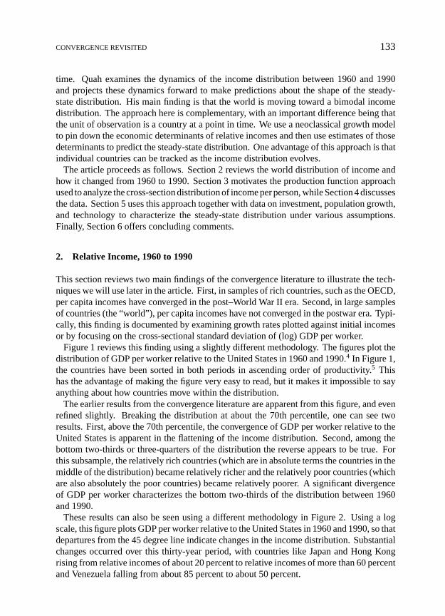
Figure 1 reviews this finding using a slightly different methodology. The figures plot thedistribution of GDP per worker relative to the United States in 1960 and 1990.4 In Figure 1,the countries have been sorted in both periods in ascending order of productivity.5 Thishas the advantage of making the figure very easy to read, but it makes it impossible to sayanything about how countries move within the distribution.

The earlier results from the convergence literature are apparent from this figure, and evenrefined slightly. Breaking the distribution at about the 70th percentile, one can see tworesults. First, above the 70th percentile, the convergence of GDP per worker relative to theUnited States is apparent in the flattening of the income distribution. Second, among thebottom two-thirds or three-quarters of the distribution the reverse appears to be true. Forthis subsample, the relatively rich countries (which are in absolute terms the countries in themiddle of the distribution) became relatively richer and the relatively poor countries (whichare also absolutely the poor countries) became relatively poorer. A significant divergenceof GDP per worker characterizes the bottom two-thirds of the distribution between 1960and 1990.

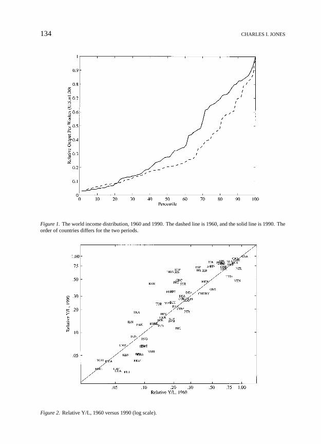
These results can also be seen using a different methodology in Figure 2. Using a logscale, this figure plots GDP per worker relative to the United States in 1960 and 1990, so thatdepartures from the 45 degree line indicate changes in the income distribution. Substantialchanges occurred over this thirty-year period, with countries like Japan and Hong Kongrising from relative incomes of about 20 percent to relative incomes of more than 60 percentand Venezuela falling from about 85 percent to about 50 percent.


Figure 1. The world income distribution, 1960 and 1990. The dashed line is 1960, and the solid line is 1990. Theorder of countries differs for the two periods.

Figure 2. Relative Y/L, 1960 versus 1990 (log scale).


3. Theory

The goal of the remainder of this article is to add a third dimension to the analysis inFigures 1 and 2 to reflect the steady-state distribution of per capita income. This sectiondescribes how we use economic theory to estimate this distribution. The economic theoryis based on a variation of the neoclassical growth model that contains elements of modelsby Mankiw, Romer, and Weil (1992) and Lucas (1988).

Let outputY in the economy be produced by physical capitalK and skilled laborHaccording to

Y(t) = K (t)α(A(t)H(t))1−α, (1)

whereA represents labor-augmenting total factor productivity. Skilled labor input is givenby

H(t) = eφS(t)L(t), (2)

whereL is raw labor input andS is time devoted to skill accumulation by a representativemember of the labor force.

Several aspects of this way of modeling human capital deserve mention. First, interpretingS as years of schooling,φ is the Mincerian rate of return to a year of schooling (Mincer,1974). An additional year of schooling increases “effective” labor input by 100φ percentand therefore increases the wage by the same amount. Constant returns to scale and theimplication that factor payments exhaust output is preserved here by assuming that thehuman capital is embodied in labor. The exponential structure assumed in the model istraditional in labor economies.6 Second, we assume there is only a single “type” of laborinput. This is motivated by data considerations: in a large sample of countries, we onlyobserve average years of schooling for the entire labor force. This makes it difficult todivide labor input into “skilled” and “unskilled,” for example.7 Finally, in this infinitehorizon setup, individuals can spend their time working or accumulating skill, as in Lucas(1988). That is, we interpretS as the fraction of an individual’s time endowment spentaccumulating skill each period. In this sense,S is more like an investment rate than acapital stock. For example, it is constant along a balanced growth path, rather than growingwith the economy.8

Letting lowercase letters denote variables normalized by the size of the labor force (sothath ≡ eφS for example), output per worker is given by

y(t) = k(t)α(A(t)h(t))1−α. (3)

Physical capital per worker evolves according to

k(t) = sK (t)y(t)− (n(t)+ δ)k(t), (4)

wheresK is the investment rate,n is the rate of population growth, andδ is a constant rateof depreciation.

Now consider solving for a balanced growth path, defined as a situation in which (1)all variables grow at constant rates and (2) the physical investment rate, the fraction of


time spent accumulating skill, and the population growth rate are constant. It is easy toshow that along such a balanced growth path, the growth rates ofy andk are equal to thegrowth rate ofA, which we will denoteg, while h is constant. We will take the growthrateg as exogenously given, noting that it could be determined by an R&D process in amore complicated model and still be exogenous to policy (as in Jones, 1995). We will alsoassume the existence of a balanced growth path instead of specifying exactly howsK , S,andn are determined.

It is then straightforward to solve for the value of per capita output along a balancedgrowth path:

y∗(t) =(

sK

n+ g+ δ) α

1−αh A∗(t), (5)

where time indices have been dropped from variables that are constant, and an asterisk (*)is used to signify the balanced growth path fory andA.

It only makes sense to think about the steady-state distribution of per capita income ifall economies are growing at the same rate. In the context of the neoclassical model, thisrequires the exogenous growth rate of technology to be the same in the long run for eachcountry, which we will now assume. How reasonable is such an assumption? At somelevel it seems plausible. For example, if technological progress is the engine of growth,one might expect that technology transfer will keep countries from diverging infinitely, andone way of interpreting this statement is that the growth rates will ultimately be the same.Indeed, in recent models by Eaton and Kortum (1994), Barro and Sala-i-Martin (1997),and Bernard and Jones (1996b) this is the case. Notice that we do not require the levelsof technology to be the same across countries or the growth rates to be the same along atransition path to the steady state.

Under the assumption that all countries asymptotically have the same growth rate oftechnology, we can consider relative per capita incomey∗ ≡ y∗(t)/y∗U S(t):

y∗ = ξα

1−αK hA∗, (6)

where the tildes are used to denote the variables considered relative to the United States andξK ≡ sK /(n+g+δ). Asymptotically, the distribution of relative incomes is nondegenerateand characterized by the elements of equation (6).

This equation summarizes an important prediction at the heart of analysis based on aproduction function and growth accounting. The steady-state distribution of (relative) percapita income is identically a function of the investment rates for physical and human capital,relative TFP levels, and population growth rates. In this approach, no other variables arerequired to estimate the steady-state distribution. Rather, variables such as preferences,taxes and subsidies, institutional differences, and political uncertainty should affect thesteady-state distribution only through one of these other variables.

4. Determinants of the Steady State

Equation (6) tells us how to calculate the long-run distribution of per capita income. Toperform this calculation, however, we need data on the parameters (which will be assumed


to be constant across countries)α, φ, andg+δ; and for the variables (which will be allowedto vary across countries),n, sK , S, andA.

4.1. The Data

In obtaining the parameters related to the shape of the production function, we assume aneoclassical production function without externalities and appeal to estimates previouslyobtained by the literature. For the exponent on physical capital, we choose the valueα = 1/3, which matches capital’s share in income for a number of countries and is areasonable value based on empirical studies by Mankiw, Romer, and Weil (1992) and Islam(1995), among others.9 For the coefficient on schooling, we follow Hall and Jones (1996)and appeal to the extensive literature estimating Mincerian coefficients for a wide rangeof countries. Based on the review of these studies by Psacharopoulos (1994), we chooseφ = .10.10 We will assume thatg + δ = .075. The results presented below are robustto small changes in these parameters. While there is still substantial debate within theliterature about the shape of aggregate production function, the neoclassical model is auseful benchmark. Indeed, if one finds some of the results implausible, this may be viewedas a test of the neoclassical approach.

For the remaining variables, nothing in the analysis hinges on whether they are endoge-nously or exogenously determined. We simply require estimates of the steady-state valueof sK , S, n, and A for each country. Of course, in practice it is very difficult to determinethe steady-state values using fundamentals such as preferences, taxes, political instability,and so on. Instead, we proceed in two directions. The first direction is to use recent datafrom each country to proxy for the steady-state value. For example, for the investment ratesand for population growth rates, we use the data for the period 1980 to 1990 in the PWT5.6 update of the Summers and Heston (1991) data set. For the relative technology level,we use an estimate of the relative level of Harrod-neutral total factor productivity in 1990,as discussed below.

To measure the fraction of time individuals spend accumulating skill, we use the educa-tional attainment data assembled by Barro and Lee (1993).11 One advantage of this measureis that there is a natural way to forecast the future stock of human capital measured as yearsof schooling. Enrollment rates of the young today, which are readily observed, determinethe average educational attainment of the labor force in the future. Therefore, in forecast-ing h, we take the observed enrollment rates from the 1980s and assume these representsteady-state enrollment rates.12

One way of viewing this analysis is as predicting where countries are headed based onthe current state of investment rates, population growth rates, and technologies. However,the current state of these variables may be strongly correlated with their long-run values.This view of the data is consistent with the recent study by Easterly, Kremer, Pritchett, andSummers (1993). These authors argue that while differences in growth rates do not showmuch persistence across decades, differences in the right-hand-side variables of growthregressions—which reflect the underlying determinants of relative income in the long-run—do show substantial persistence. They note, for example, that primary and secondaryschool enrollment rates are among the most persistent variables in the Barro (1991) growth


regression: the correlation across decades for a large sample of countries is noticeablyhigher than 0.8.13 Applying their methodology to physical investment rates for the samplesconsidered here, the correlations across decades are also uniformly above 0.8. This suggeststhat recent data on the determinants of steady-state income may do a good job of predictingtheir long-run values.

While this first direction receives primary emphasis below, we also consider the robustnessof these results by using additional economic theory to determine steady-state values. Forexample, in one alternative we require the rates of return to physical capital to be equal toreflect a perfect capital mobility assumption. Another examines the behavior of relativeincomes after countries have undergone a “demographic transition” that reduces populationgrowth rates to a common value of 1 percent per year.

A shortcoming of the general approach taken in this article is that there is no modelof the endogenous (and presumably related) responses of investment rates, schooling, andtechnology to underlying fundamentals. An alternative and more ambitious approach wouldbe to specify the fundamentals that determine these variables within the context of a theory,to forecast the future of the fundamentals, and then to use the theory to predict the behaviorof relative incomes. The present exercise can be viewed as a first step in this direction usinga well-studied model.

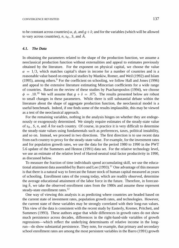
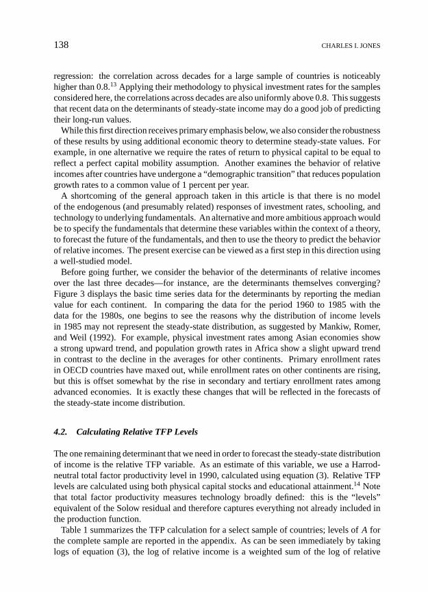
Before going further, we consider the behavior of the determinants of relative incomesover the last three decades—for instance, are the determinants themselves converging?Figure 3 displays the basic time series data for the determinants by reporting the medianvalue for each continent. In comparing the data for the period 1960 to 1985 with thedata for the 1980s, one begins to see the reasons why the distribution of income levelsin 1985 may not represent the steady-state distribution, as suggested by Mankiw, Romer,and Weil (1992). For example, physical investment rates among Asian economies showa strong upward trend, and population growth rates in Africa show a slight upward trendin contrast to the decline in the averages for other continents. Primary enrollment ratesin OECD countries have maxed out, while enrollment rates on other continents are rising,but this is offset somewhat by the rise in secondary and tertiary enrollment rates amongadvanced economies. It is exactly these changes that will be reflected in the forecasts ofthe steady-state income distribution.

4.2. Calculating Relative TFP Levels

The one remaining determinant that we need in order to forecast the steady-state distributionof income is the relative TFP variable. As an estimate of this variable, we use a Harrod-neutral total factor productivity level in 1990, calculated using equation (3). Relative TFPlevels are calculated using both physical capital stocks and educational attainment.14 Notethat total factor productivity measures technology broadly defined: this is the “levels”equivalent of the Solow residual and therefore captures everything not already included inthe production function.

Table 1 summarizes the TFP calculation for a select sample of countries; levels ofA forthe complete sample are reported in the appendix. As can be seen immediately by takinglogs of equation (3), the log of relative income is a weighted sum of the log of relative


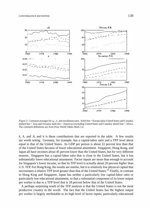
Figure 3. Continent averages forsK , n, and enrollment rates. Solid line = Europe (plus United States and Canada);dashed line = Asia and Oceania; dash-dot = Americas (excluding United States and Canada); dotted line = Africa.The continent definitions are from Penn World Tables Mark 5.6.

k, h, and A, and it is these contributions that are reported in the table. A few resultsare worth noting. Germany, for example, has a capital-labor ratio and a TFP level aboutequal to that of the United States. Its GDP per person is about 22 percent less than thatof the United States because of lower educational attainment. Singapore, Hong Kong, andJapan all have incomes about 45 percent lower than the United States, but for very differentreasons. Singapore has a capital-labor ratio that is close to the United States, but it hassubstantially lower educational attainment. Factor inputs are more than enough to accountfor Singapore’s lower income, so that its TFP level is actually about 20 percenthigherthanU.S. TFP. For Hong King, the results are similar, but it is relatively low physical capital thatnecessitates a relative TFP level greater than that of the United States.15 Finally, in contrastto Hong King and Singapore, Japan has neither a particularly low capital-labor ratio orparticularly low educational attainment, so that a substantial component of its lower outputper worker is due to a TFP level that is 18 percent below that of the United States.

A perhaps surprising result of the TFP analysis is that the United States is not the mostproductive country in the world. The fact that the United States has the highest outputper worker is largely attributable to its high level of factor inputs, particularly educational


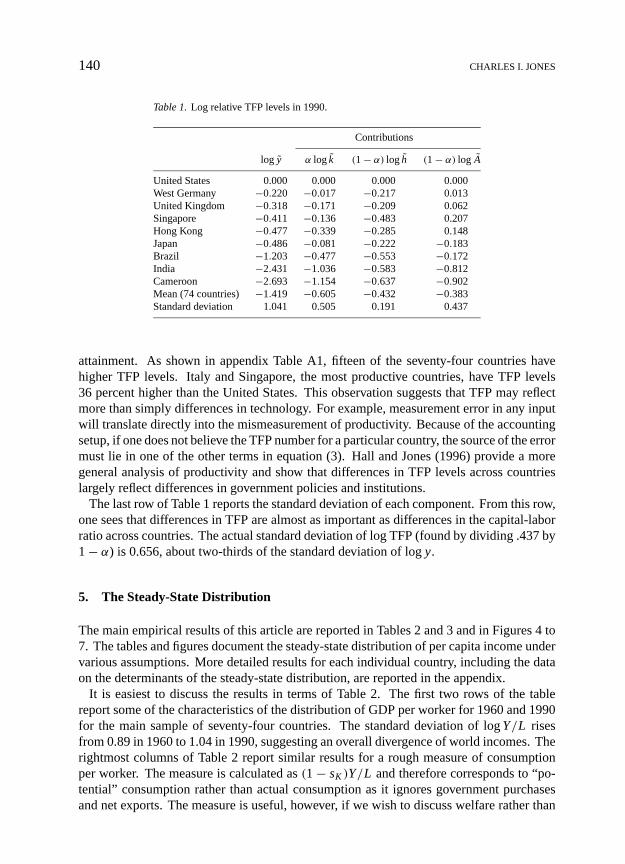
Table 1.Log relative TFP levels in 1990.

Contributions

log y α log k (1− α) log h (1− α) log A

United States 0.000 0.000 0.000 0.000West Germany −0.220 −0.017 −0.217 0.013United Kingdom −0.318 −0.171 −0.209 0.062Singapore −0.411 −0.136 −0.483 0.207Hong Kong −0.477 −0.339 −0.285 0.148Japan −0.486 −0.081 −0.222 −0.183Brazil −1.203 −0.477 −0.553 −0.172India −2.431 −1.036 −0.583 −0.812Cameroon −2.693 −1.154 −0.637 −0.902Mean (74 countries) −1.419 −0.605 −0.432 −0.383Standard deviation 1.041 0.505 0.191 0.437

attainment. As shown in appendix Table A1, fifteen of the seventy-four countries havehigher TFP levels. Italy and Singapore, the most productive countries, have TFP levels36 percent higher than the United States. This observation suggests that TFP may reflectmore than simply differences in technology. For example, measurement error in any inputwill translate directly into the mismeasurement of productivity. Because of the accountingsetup, if one does not believe the TFP number for a particular country, the source of the errormust lie in one of the other terms in equation (3). Hall and Jones (1996) provide a moregeneral analysis of productivity and show that differences in TFP levels across countrieslargely reflect differences in government policies and institutions.

The last row of Table 1 reports the standard deviation of each component. From this row,one sees that differences in TFP are almost as important as differences in the capital-laborratio across countries. The actual standard deviation of log TFP (found by dividing .437 by1− α) is 0.656, about two-thirds of the standard deviation of logy.

5. The Steady-State Distribution

The main empirical results of this article are reported in Tables 2 and 3 and in Figures 4 to7. The tables and figures document the steady-state distribution of per capita income undervarious assumptions. More detailed results for each individual country, including the dataon the determinants of the steady-state distribution, are reported in the appendix.

It is easiest to discuss the results in terms of Table 2. The first two rows of the tablereport some of the characteristics of the distribution of GDP per worker for 1960 and 1990for the main sample of seventy-four countries. The standard deviation of logY/L risesfrom 0.89 in 1960 to 1.04 in 1990, suggesting an overall divergence of world incomes. Therightmost columns of Table 2 report similar results for a rough measure of consumptionper worker. The measure is calculated as(1− sK )Y/L and therefore corresponds to “po-tential” consumption rather than actual consumption as it ignores government purchasesand net exports. The measure is useful, however, if we wish to discuss welfare rather than


Table 2.Evolution of the income distribution, full sample.

GDP Consumption

Method σ U.S.% R2 σ U.S.%

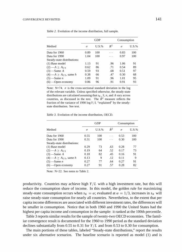
Data for 1960 0.89 100 · · · 0.83 100Data for 1990 1.04 100 · · · 0.97 100Steady-state distributions:(1) Base model 1.13 91 .96 1.06 91(2) —A ≥ AU S 0.62 86 .71 0.54 89(3) —SameA 0.59 93 .68 0.51 97(4) —A ≥ AU S, sameh 0.38 66 .47 0.30 68(5) —Samen 1.09 91 .96 1.01 95(6) —Open economy 0.86 96 .91 0.91 93

Note: N=74. σ is the cross-sectional standard deviation in the logof the relevant variable. Unless specified otherwise, the steady-statedistributions are calculated assuming thatsK , S, n, andA vary acrosscountries, as discussed in the text. TheR2 measure reflects thefraction of the variance of 1990 logY/L “explained” by the steady-state distribution. See text.

Table 3.Evolution of the income distribution, OECD.

GDP Consumption

Method σ U.S.% R2 σ U.S.%

Data for 1960 0.55 100 · · · 0.53 100Data for 1990 0.31 100 · · · 0.30 100Steady-state distributions:(1) Base model 0.29 73 .63 0.28 77(2) —A ≥ AU S 0.19 64 .52 0.17 73(3) —SameA 0.18 82 .45 0.16 91(4) —A ≥ AU S, sameh 0.13 9 .12 0.11 9(5) —Samen 0.27 77 .64 0.27 91(6) —Open economy 0.27 91 .57 0.28 82

Note: N=22. See notes to Table 2.

productivity. Countries may achieve highY/L with a high investment rate, but this willreduce the consumption share of income. In this model, the golden rule for maximizingsteady-state consumption occurs whensK = α; evaluated atα = 1/3, increases insK willraise steady-state consumption for nearly all countries. Nevertheless, to the extent that percapita income differences are associated with different investment rates, the differences willbe smaller in consumption. Notice that in both 1960 and 1990 the United States had thehighest per capita income and consumption in the sample: it ranked at the 100th percentile.

Table 3 reports similar results for the sample of twenty-two OECD economies. The famil-iar convergence result is documented for the 1960 to 1990 period as the standard deviationdeclines substantially from 0.55 to 0.31 forY/L and from 0.53 to 0.30 for consumption.

The main portions of these tables, labeled “Steady-state distributions,” report the resultsunder six alternative scenarios. The baseline scenario is reported as model (1) and is


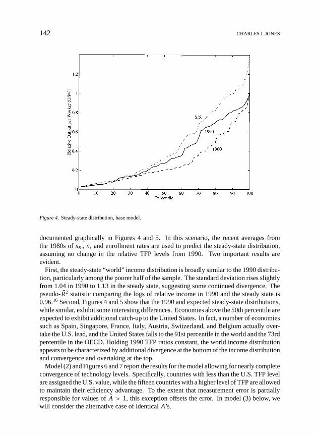
Figure 4. Steady-state distribution, base model.

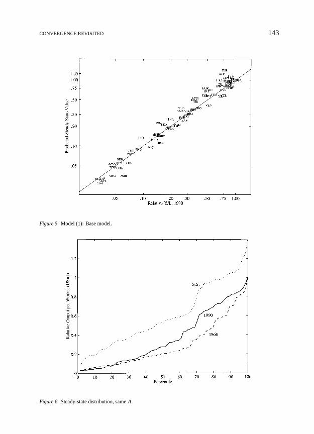
documented graphically in Figures 4 and 5. In this scenario, the recent averages fromthe 1980s ofsK , n, and enrollment rates are used to predict the steady-state distribution,assuming no change in the relative TFP levels from 1990. Two important results areevident.

First, the steady-state “world” income distribution is broadly similar to the 1990 distribu-tion, particularly among the poorer half of the sample. The standard deviation rises slightlyfrom 1.04 in 1990 to 1.13 in the steady state, suggesting some continued divergence. Thepseudo-R2 statistic comparing the logs of relative income in 1990 and the steady state is0.96.16 Second, Figures 4 and 5 show that the 1990 and expected steady-state distributions,while similar, exhibit some interesting differences. Economies above the 50th percentile areexpected to exhibit additional catch-up to the United States. In fact, a number of economiessuch as Spain, Singapore, France, Italy, Austria, Switzerland, and Belgium actually over-take the U.S. lead, and the United States falls to the 91st percentile in the world and the 73rdpercentile in the OECD. Holding 1990 TFP ratios constant, the world income distributionappears to be characterized by additional divergence at the bottom of the income distributionand convergence and overtaking at the top.

Model (2) and Figures 6 and 7 report the results for the model allowing for nearly completeconvergence of technology levels. Specifically, countries with less than the U.S. TFP levelare assigned the U.S. value, while the fifteen countries with a higher level of TFP are allowedto maintain their efficiency advantage. To the extent that measurement error is partiallyresponsible for values ofA > 1, this exception offsets the error. In model (3) below, wewill consider the alternative case of identicalA’s.


Figure 5. Model (1): Base model.

Figure 6. Steady-state distribution, sameA.


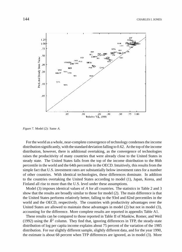
Figure 7. Model (2): SameA.

For the world as a whole, near-complete convergence of technology condenses the incomedistribution significantly, with the standard deviation falling to 0.62. At the top of the incomedistribution, however, there is additional overtaking, as the convergence of technologiesraises the producitivity of many countries that were already close to the United States insteady state. The United States falls from the top of the income distribution to the 86thpercentile in the world and the 64th percentile in the OECD. Intuitively, this results from thesimple fact that U.S. investment rates are substantially below investment rates for a numberof other countries. With identical technologies, these differences dominate. In additionto the countries overtaking the United States according to model (1), Japan, Korea, andFinland all rise to more than the U.S. level under these assumptions.

Model (3) imposes identical values ofA for all countries. The statistics in Table 2 and 3show that the results are broadly similar to those for model (2). The main difference is thatthe United States performs relatively better, falling to the 93rd and 82nd percentiles in theworld and the OECD, respectively. The countries with productivity advantages over theUnited States are allowed to maintain these advantages in model (2) but not in model (3),accounting for the difference. More complete results are reported in appendix Table A1.

These results can be compared to those reported in Table II of Mankiw, Romer, and Weil(1992) using theR2 column. They find that, ignoring differences in TFP, the steady-statedistribution of log per capita income explains about 75 percent of the variation of the 1985distribution. For our slightly different sample, slightly different data, and for the year 1990,the estimate is about 68 percent when TFP differences are ignored, as in model (3). More


generally, theR2 statistics indicate how similar the steady-state distribution is to the 1990distribution.

5.1. Alternative Scenarios

Model (4) considers what happens to the distribution if relative technology levels convergeto the technology level of the United States and the countries have the same educationalattainment. Thus, this scenario downplays determinants in which the United States per-forms well and plays up investment and population growth, determinants for which U.S.performance is relatively weak. Not surprisingly, this alters the distribution significantly.First, there is substantial convergence in the income distribution; the standard deviationfalls from 1.04 in 1990 to only 0.38. Second, this shift leads to a number of countriesovertaking the United States in productivity, as the United States falls to the 66th percentilein the world and only the 9th percentile in the OECD. Results for specific countries may befound in the appendix.

Model (5) is a simple way of examining the importance of a demographic transition. Inthis model, all countries have the same population growth rate of 1 percent in steady state.According to the results in Tables 2 and 3, this change has very little impact on the results;the statistics are very close to those for the base scenario in model (1). The explanationfor the insensitivity of the results to population growth is easily seen by computing thesemi-elasticity of income with respect to population growth from equation (6). For typicalparameter values, this elasticity is very small.

Model (6) considers the open economy scenario. According to this scenario, the marginalproducts of physical capital are equated across countries. This means that(n+ g+ δ)/sK

is equal across countries.17 Notice that this scenario emphasizes differences in TFP andhuman capital investment as determinants of the steady-state distribution. These are thedeterminants for which the United States performs relatively well, and this intuition isconfirmed in the results. Under this scenario, although the standard deviation falls backto its 1960 level, the United States remains very close to the top of the world incomedistribution.

5.2. The Return to Capital

The results so far for the steady-state distribution of per capita income can be partiallysummarized as follows. Recent data on investment rates, educational attainment, populationgrowth rates, and relative technologies suggest that the long-run distribution of incomeinvolves the United States falling from its leadership position. However, an open economyscenario in which the marginal products of physical capital are equalized across countriesmitigates this change.

This section considers the differences in the rates of return to capital across countries in1990 and in the steady state according to the various models. The rate of return to capitalin the steady state is given byα(n + g + δ)/sK . That is, it varies across countries onlybecause of variation in population growth and the physical investment rate. In the context


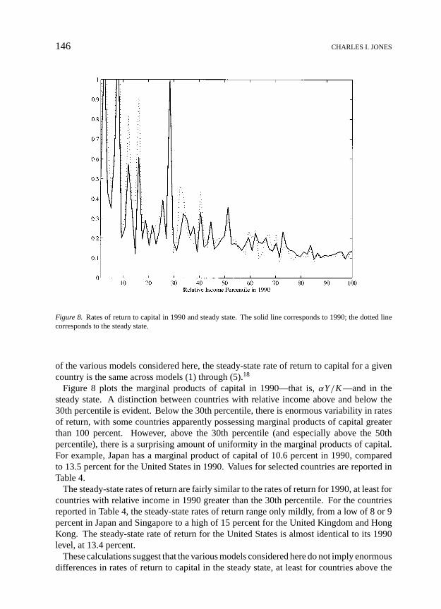
Figure 8. Rates of return to capital in 1990 and steady state. The solid line corresponds to 1990; the dotted linecorresponds to the steady state.

of the various models considered here, the steady-state rate of return to capital for a givencountry is the same across models (1) through (5).18

Figure 8 plots the marginal products of capital in 1990—that is,αY/K—and in thesteady state. A distinction between countries with relative income above and below the30th percentile is evident. Below the 30th percentile, there is enormous variability in ratesof return, with some countries apparently possessing marginal products of capital greaterthan 100 percent. However, above the 30th percentile (and especially above the 50thpercentile), there is a surprising amount of uniformity in the marginal products of capital.For example, Japan has a marginal product of capital of 10.6 percent in 1990, comparedto 13.5 percent for the United States in 1990. Values for selected countries are reported inTable 4.

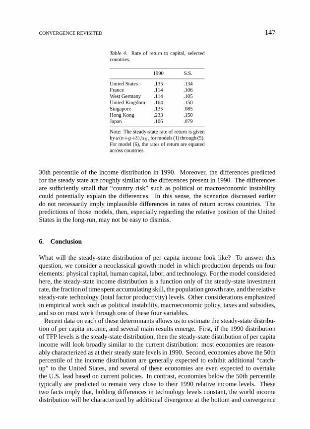
The steady-state rates of return are fairly similar to the rates of return for 1990, at least forcountries with relative income in 1990 greater than the 30th percentile. For the countriesreported in Table 4, the steady-state rates of return range only mildly, from a low of 8 or 9percent in Japan and Singapore to a high of 15 percent for the United Kingdom and HongKong. The steady-state rate of return for the United States is almost identical to its 1990level, at 13.4 percent.

These calculations suggest that the various models considered here do not imply enormousdifferences in rates of return to capital in the steady state, at least for countries above the


Table 4. Rate of return to capital, selectedcountries.

1990 S.S.

United States .135 .134France .114 .106West Germany .114 .105United Kingdom .164 .150Singapore .135 .085Hong Kong .233 .150Japan .106 .079

Note: The steady-state rate of return is givenbyα(n+g+δ)/sK , for models (1) through (5).For model (6), the rates of return are equatedacross countries.

30th percentile of the income distribution in 1990. Moreover, the differences predictedfor the steady state are roughly similar to the differences present in 1990. The differencesare sufficiently small that “country risk” such as political or macroeconomic instabilitycould potentially explain the differences. In this sense, the scenarios discussed earlierdo not necessarily imply implausible differences in rates of return across countries. Thepredictions of those models, then, especially regarding the relative position of the UnitedStates in the long-run, may not be easy to dismiss.

6. Conclusion

What will the steady-state distribution of per capita income look like? To answer thisquestion, we consider a neoclassical growth model in which production depends on fourelements: physical capital, human capital, labor, and technology. For the model consideredhere, the steady-state income distribution is a function only of the steady-state investmentrate, the fraction of time spent accumulating skill, the population growth rate, and the relativesteady-rate technology (total factor productivity) levels. Other considerations emphasizedin empirical work such as political instability, macroeconomic policy, taxes and subsidies,and so on must work through one of these four variables.

Recent data on each of these determinants allows us to estimate the steady-state distribu-tion of per capita income, and several main results emerge. First, if the 1990 distributionof TFP levels is the steady-state distribution, then the steady-state distribution of per capitaincome will look broadly similar to the current distribution: most economies are reason-ably characterized as at their steady state levels in 1990. Second, economies above the 50thpercentile of the income distribution are generally expected to exhibit additional “catch-up” to the United States, and several of these economies are even expected to overtakethe U.S. lead based on current policies. In contrast, economies below the 50th percentiletypically are predicted to remain very close to their 1990 relative income levels. Thesetwo facts imply that, holding differences in technology levels constant, the world incomedistribution will be characterized by additional divergence at the bottom and convergence


and overtaking at the top. Third differences in TFP levels across countries are substantial,and changes in relative TFP levels can have important effects on the steady-state incomedistribution. Finally, current dynamics imply a future income distribution in which theUnited States is surpassed by a number of other countries. For example, the main modelssuggest that the United States would fall from the 100th percentile to the 86th percentile inthe income distribution. Countries such as France, Singapore, and Spain are expected tohave incomes ranging from 115 percent to 140 percent of U.S. income under this scenario.The explanation of this result is twofold. First, the U.S. lead in educational attainmentcannot completely make up for its low investment rate. Second, a number of countries havehigher TFP levels than the United States.

Given that the results are partially driven by low levels of physical investment in theUnited States, a natural question is whether the steady-state distributions imply implausiblylarge differences in the rates of return to investment. The final part of the article argues thatthis is not the case. The steady-state differences in rates of return are surprisingly small andlook very much like the differences observed in 1990. There may be little incentive, then,for investment rates in physical capital among advanced economies to converge.

Data Appendix

This appendix discusses the data used in the paper. “SH” refers to the Penn World TablesMark 5.6 of Summers and Heston (1991) obtained via ftp from nber.harvard.edu.

GDP Per Worker

The “rgdpw” series from the SH.sK is the “i” series for investment rates from SH, averagedfrom 1980 to 1990.n is population growth rates, calculated as the change in the log of theSH population series, averaged from 1980 to 1990. Labor force growth rates are not usedbecause of discrete breaks in the trend in the labor force series for a number of Africancountries around the year 1986 (for example, Ghana, Kenya, Nigeria, Mali, and Zimbabwe).

Physical Capital Stocks

The capital stock is calculated by summing investment from its earliest available year(1960 or before) to 1990 using a depreciation rate of 6 percent and an initial capital stockdetermined by the initial investment rate divided by the growth rate of investment duringthe subsequent ten years. Because the initial stock will have had at least thirty years todepreciate, our capital stock measure is quite insensitive to the initial value.

Educational Attainment (S)

Educational attainment is used in two ways. For computing the total factor productivitylevel, the 1985 levels from Barro and Lee (1993) are used because no 1990 data is available.


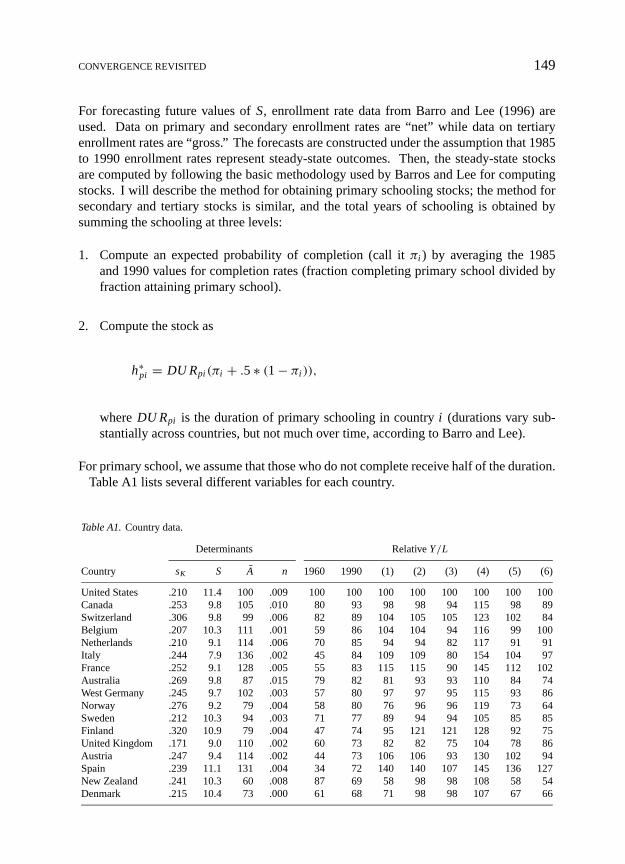
For forecasting future values ofS, enrollment rate data from Barro and Lee (1996) areused. Data on primary and secondary enrollment rates are “net” while data on tertiaryenrollment rates are “gross.” The forecasts are constructed under the assumption that 1985to 1990 enrollment rates represent steady-state outcomes. Then, the steady-state stocksare computed by following the basic methodology used by Barros and Lee for computingstocks. I will describe the method for obtaining primary schooling stocks; the method forsecondary and tertiary stocks is similar, and the total years of schooling is obtained bysumming the schooling at three levels:

1. Compute an expected probability of completion (call itπi ) by averaging the 1985and 1990 values for completion rates (fraction completing primary school divided byfraction attaining primary school).

2. Compute the stock as

h∗pi = DU Rpi (πi + .5 ∗ (1− πi )),

whereDU Rpi is the duration of primary schooling in countryi (durations vary sub-stantially across countries, but not much over time, according to Barro and Lee).

For primary school, we assume that those who do not complete receive half of the duration.Table A1 lists several different variables for each country.

Table A1.Country data.

Determinants RelativeY/L

Country sK S A n 1960 1990 (1) (2) (3) (4) (5) (6)

United States .210 11.4 100 .009 100 100 100 100 100 100 100 100Canada .253 9.8 105 .010 80 93 98 98 94 115 98 89Switzerland .306 9.8 99 .006 82 89 104 105 105 123 102 84Belgium .207 10.3 111 .001 59 86 104 104 94 116 99 100Netherlands .210 9.1 114 .006 70 85 94 94 82 117 91 91Italy .244 7.9 136 .002 45 84 109 109 80 154 104 97France .252 9.1 128 .005 55 83 115 115 90 145 112 102Australia .269 9.8 87 .015 79 82 81 93 93 110 84 74West Germany .245 9.7 102 .003 57 80 97 97 95 115 93 86Norway .276 9.2 79 .004 58 80 76 96 96 119 73 64Sweden .212 10.3 94 .003 71 77 89 94 94 105 85 85Finland .320 10.9 79 .004 47 74 95 121 121 128 92 75United Kingdom .171 9.0 110 .002 60 73 82 82 75 104 78 86Austria .247 9.4 114 .002 44 73 106 106 93 130 102 94Spain .239 11.1 131 .004 34 72 140 140 107 145 136 127New Zealand .241 10.3 60 .008 87 69 58 98 98 108 58 54Denmark .215 10.4 73 .000 61 68 71 98 98 107 67 66


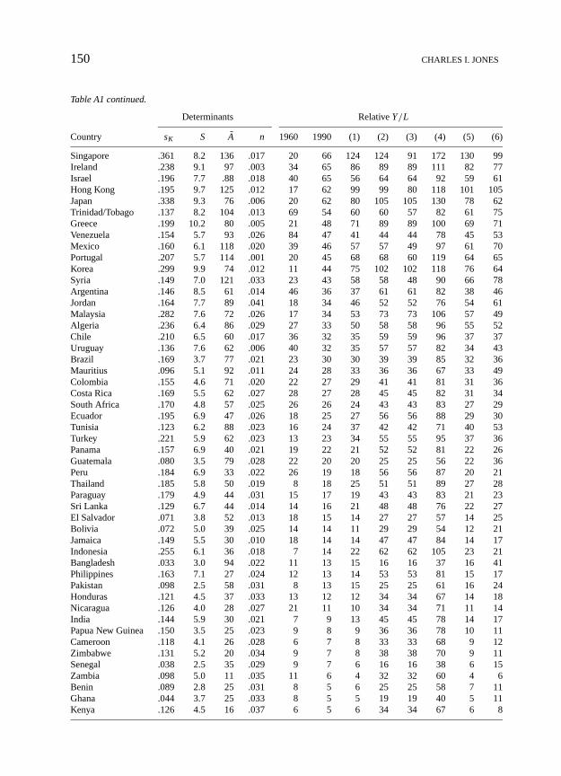
Table A1 continued.


Country sK S A n 1960 1990 (1) (2) (3) (4) (5) (6)

Singapore .361 8.2 136 .017 20 66 124 124 91 172 130 99Ireland .238 9.1 97 .003 34 65 86 89 89 111 82 77Israel .196 7.7 .88 .018 40 65 56 64 64 92 59 61Hong Kong .195 9.7 125 .012 17 62 99 99 80 118 101 105Japan .338 9.3 76 .006 20 62 80 105 105 130 78 62Trinidad/Tobago .137 8.2 104 .013 69 54 60 60 57 82 61 75Greece .199 10.2 80 .005 21 48 71 89 89 100 69 71Venezuela .154 5.7 93 .026 84 47 41 44 44 78 45 53Mexico .160 6.1 118 .020 39 46 57 57 49 97 61 70Portugal .207 5.7 114 .001 20 45 68 68 60 119 64 65Korea .299 9.9 74 .012 11 44 75 102 102 118 76 64Syria .149 7.0 121 .033 23 43 58 58 48 90 66 78Argentina .146 8.5 61 .014 46 36 37 61 61 82 38 46Jordan .164 7.7 89 .041 18 34 46 52 52 76 54 61Malaysia .282 7.6 72 .026 17 34 53 73 73 106 57 49Algeria .236 6.4 86 .029 27 33 50 58 58 96 55 52Chile .210 6.5 60 .017 36 32 35 59 59 96 37 37Uruguay .136 7.6 62 .006 40 32 35 57 57 82 34 43Brazil .169 3.7 77 .021 23 30 30 39 39 85 32 36Mauritius .096 5.1 92 .011 24 28 33 36 36 67 33 49Colombia .155 4.6 71 .020 22 27 29 41 41 81 31 36Costa Rica .169 5.5 62 .027 28 27 28 45 45 82 31 34South Africa .170 4.8 57 .025 26 26 24 43 43 83 27 29Ecuador .195 6.9 47 .026 18 25 27 56 56 88 29 30Tunisia .123 6.2 88 .023 16 24 37 42 42 71 40 53Turkey .221 5.9 62 .023 13 23 34 55 55 95 37 36Panama .157 6.9 40 .021 19 22 21 52 52 81 22 26Guatemala .080 3.5 79 .028 22 20 20 25 25 56 22 36Peru .184 6.9 33 .022 26 19 18 56 56 87 20 21Thailand .185 5.8 50 .019 8 18 25 51 51 89 27 28Paraguay .179 4.9 44 .031 15 17 19 43 43 83 21 23Sri Lanka .129 6.7 44 .014 14 16 21 48 48 76 22 27El Salvador .071 3.8 52 .013 18 15 14 27 27 57 14 25Bolivia .072 5.0 39 .025 14 14 11 29 29 54 12 21Jamaica .149 5.5 30 .010 18 14 14 47 47 84 14 17Indonesia .255 6.1 36 .018 7 14 22 62 62 105 23 21Bangladesh .033 3.0 94 .022 11 13 15 16 16 37 16 41Philippines .163 7.1 27 .024 12 13 14 53 53 81 15 17Pakistan .098 2.5 58 .031 8 13 15 25 25 61 16 24Honduras .121 4.5 37 .033 13 12 12 34 34 67 14 18Nicaragua .126 4.0 28 .027 21 11 10 34 34 71 11 14India .144 5.9 30 .021 7 9 13 45 45 78 14 17Papua New Guinea .150 3.5 25 .023 9 8 9 36 36 78 10 11Cameroon .118 4.1 26 .028 6 7 8 33 33 68 9 12Zimbabwe .131 5.2 20 .034 9 7 8 38 38 70 9 11Senegal .038 2.5 35 .029 9 7 6 16 16 38 6 15Zambia .098 5.0 11 .035 11 6 4 32 32 60 4 6Benin .089 2.8 25 .031 8 5 6 25 25 58 7 11Ghana .044 3.7 25 .033 8 5 5 19 19 40 5 11Kenya .126 4.5 16 .037 6 5 6 34 34 67 6 8


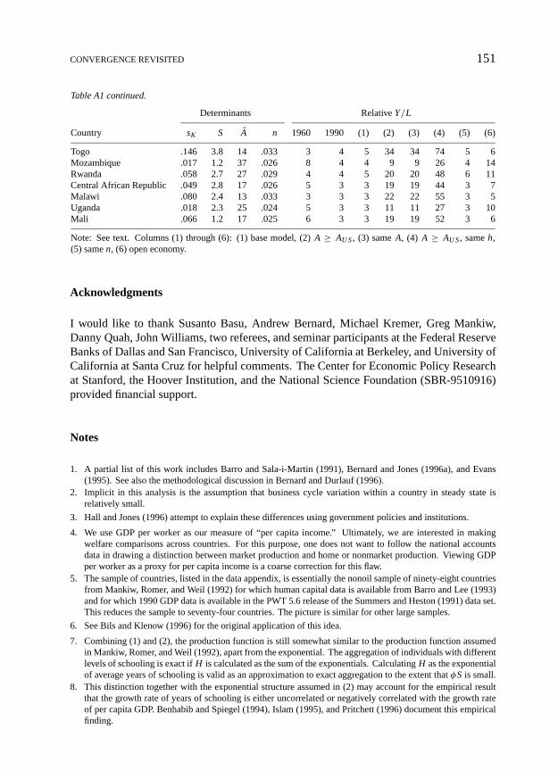
Table A1 continued.


Country sK S A n 1960 1990 (1) (2) (3) (4) (5) (6)

Togo .146 3.8 14 .033 3 4 5 34 34 74 5 6Mozambique .017 1.2 37 .026 8 4 4 9 9 26 4 14Rwanda .058 2.7 27 .029 4 4 5 20 20 48 6 11Central African Republic .049 2.8 17 .026 5 3 3 19 19 44 3 7Malawi .080 2.4 13 .033 3 3 3 22 22 55 3 5Uganda .018 2.3 25 .024 5 3 3 11 11 27 3 10Mali .066 1.2 17 .025 6 3 3 19 19 52 3 6

Note: See text. Columns (1) through (6): (1) base model, (2)A ≥ AU S, (3) sameA, (4) A ≥ AU S, sameh,(5) samen, (6) open economy.

Acknowledgments

I would like to thank Susanto Basu, Andrew Bernard, Michael Kremer, Greg Mankiw,Danny Quah, John Williams, two referees, and seminar participants at the Federal ReserveBanks of Dallas and San Francisco, University of California at Berkeley, and University ofCalifornia at Santa Cruz for helpful comments. The Center for Economic Policy Researchat Stanford, the Hoover Institution, and the National Science Foundation (SBR-9510916)provided financial support.

Notes

1. A partial list of this work includes Barro and Sala-i-Martin (1991), Bernard and Jones (1996a), and Evans(1995). See also the methodological discussion in Bernard and Durlauf (1996).

2. Implicit in this analysis is the assumption that business cycle variation within a country in steady state isrelatively small.

3. Hall and Jones (1996) attempt to explain these differences using government policies and institutions.

4. We use GDP per worker as our measure of “per capita income.” Ultimately, we are interested in makingwelfare comparisons across countries. For this purpose, one does not want to follow the national accountsdata in drawing a distinction between market production and home or nonmarket production. Viewing GDPper worker as a proxy for per capita income is a coarse correction for this flaw.

5. The sample of countries, listed in the data appendix, is essentially the nonoil sample of ninety-eight countriesfrom Mankiw, Romer, and Weil (1992) for which human capital data is available from Barro and Lee (1993)and for which 1990 GDP data is available in the PWT 5.6 release of the Summers and Heston (1991) data set.This reduces the sample to seventy-four countries. The picture is similar for other large samples.

6. See Bils and Klenow (1996) for the original application of this idea.

7. Combining (1) and (2), the production function is still somewhat similar to the production function assumedin Mankiw, Romer, and Weil (1992), apart from the exponential. The aggregation of individuals with differentlevels of schooling is exact ifH is calculated as the sum of the exponentials. CalculatingH as the exponentialof average years of schooling is valid as an approximation to exact aggregation to the extent thatφS is small.

8. This distinction together with the exponential structure assumed in (2) may account for the empirical resultthat the growth rate of years of schooling is either uncorrelated or negatively correlated with the growth rateof per capita GDP. Benhabib and Spiegel (1994), Islam (1995), and Pritchett (1996) document this empiricalfinding.


9. Bernard and Jones (1996a) discuss the difficulties of defining total factor productivity when the exponents ofthe production function differ across countries and suggest imposing equality as one reasonable solution.

10. Psacharopoulos reports Mincerian coefficients ranging from .068 in the OECD to .134 in Sub-Saharan Africaand an average value across countries of .101. This range seems quite small relative to what one might guessabout variation in the capital share across countries.

11. The educational attainment data is measured as years of schooling rather than as a fraction of time, but sinceour calibration ofφ is also based on years of schooling, this is appropriate.

12. The exact forecasting method is based on the method Barro and Lee (1993) use to compute educationalattainment and is discussed in the appendix.

13. See Figure 5 of their paper.

14. See the appendix for details on the construction of the capital stock. Educational attainment data are from1985 because 1990 data were not available.

15. The results for physical and human capital in Hong Kong and Singapore are consistent with Young (1992).The result for TFP is not inconsistent with Young because his results are for growth rates rather than levels.In fact, the high levels of TFP may partially explain the low growth rate.

16. TheR2 is really a pseudo-R2. It is calculated by considering the difference between the log of per capitaincome in 1990 and the log of per capita income in the steady state. The pseudo-R2 is then computed as (oneminus) the ratio of the variance of this difference to the variance of the 1990 log income.

17. For calculating consumption in the open economy scenario, it is important to distinguish between saving andinvestment. Steady-state consumption is calculated asc = (1− s)y(1− α+ αs/ i ), wheres is the saving rateandi is the open economy investment rate.

18. Of course, the open economy model equates these rates of return across countries, so that the distribution thereis degenerate.

References

Abramovitz, M. (1986). “Catching Up, Forging Ahead and Falling Behind,”Journal of Economic History46,385–406.

Barro, R. (1991). “Economic Growth in a Cross-Section of Countries,”Quarterly Journal of Economics106,407–443.

Barro, R., and J. Lee. (1993). “International Comparisons of Educational Attainment,”Journal of MonetaryEconomics32, 363–394.

Barro, R., and J. Lee. (1996). “International Data on Education,” Mimeo, Harvard University.Barro, R., and X. Sala-i-Martin. (1991). “Convergence Across States and Regions,”Brookings Papers on

Economic Activity, 107–158.Barro, R., and X. Sala-i-Martin. (1997). “Technological Diffusion, Convergence, and Growth,”Journal of

Economic Growth2, 1–26.Baumol, W.J. (1986). “Productivity Growth, Convergence and Welfare: What the Long-Run Data Show,”Amer-

ican Economic Review76, 1072–1085.Benhabib, J., and M. Spiegal. (1994). “The Role of Human Capital in Economic Development: Evidence from

Aggregate Cross-Country Data,”Journal of Monetary Economics34, 143–173.Bernard, A.B., and S.N. Durlauf. (1996). “Interpreting Tests of the Convergence Hypothesis,”Journal of

Econometrics71, 161–173.Bernard, A.B., and C.I. Jones. (1996a). “Comparing Apples to Oranges: Productivity Convergence and Measure-

ment Across Industries and Countries,”American Economic Review86, 1216–1238.Bernard, A.B., and C.I. Jones. (1996b). “Technology and Convergence,”Economic Journal106, 1037–1044.Bils, M., and P. Klenow. (1996). “Does Schooling Cause Growth or the Other Way Around?,” Mimeo, University

of Chicago Graduate School of Business.Easterly, W., M. Kremer, L. Pritchett, and L. Summers. (1993). “Good Policy or Good Luck? Country Growth

Performance and Temporary Shocks,”Journal of Monetary Economics32, 459–483.Eaton, J., and S. Kortum. (1994). “International Patenting and Technology Diffusion,” Mimeo, Boston University.Evans, P. (1995). “How Fast Do Economies Converge,” Mimeo, Ohio State University.


Hall, R.E., and C.I. Jones. (1996). “The Productivity of Nations,” NBER Working Paper No. 5812.Islam, N. (1995). “Growth Empirics: A Panel Data Approach,”Quarterly Journal of Economics110, 1127–1170.Jones, C.I. (1995). “R&D-Based Models of Economic Growth,”Journal of Political Economy103, 759–784.Lucas, R.E. (1988). “On the Mechanics of Economic Development,”Journal of Monetary Economics22, 3–42.Mankiw, N.G., D. Romer, and D. Weil. (1992). “A Contribution to the Empirics of Economic Growth,”Quarterly

Journal of Economics107, 407–438.Mincer, J. (1974).Schooling, Experience, and Earnings. New York: Columbia University Press.Pritchett, L. (1996). “Where Has All the Education Gone?,” World Bank, Policy Research Working Paper No. 1581.Psacharopoulos, G. (1994). “Returns to Investment in Education: A Global Update,”World Development22,

1325–1343.Quah, D. (1993). “Galton’s Fallacy and Tests of the Convergence Hypothesis,”Scandinavian Journal of Eco-

nomics, 95, 427–443.Quah, D. (1996). “Convergence Empirics Across Economies with (Some) Capital Mobility,”Journal of Economic

Growth, 1, 95–124.Solow, R.M. (1956). “A Contribution to the Theory of Economic Growth,”Quarterly Journal of Economics70,

65–94.Summers, R., and A. Heston. (1991). “The Penn World Table (Mark 5): An Expanded Set of International

Comparisons: 1950–1988,”Quarterly Journal of Economics106, 327–368.Young, A. (1992). “A Tale of Two Cities: Factor Accumulation and Technical Change in Hong Kong and

Singapore,” in O. Blanchard and S. Fischer (eds.),NBER Macroeconomics Annual. Cambridge, MA: MITPress.

Documents

Convergence Revisited - Stanford Universityweb.stanford.edu/~chadj/jeg1997.pdf · TFP convergence for the evolution of the income distribution. The framework in this article is the