Convergence rate of a finite volume scheme for a two dimensional convection-diffusion … · Mathematical Modelling and Numerical Analysis M2AN, Vol. 33, No 3, 1999, p. 493{516 Mod

Mathematical Modelling and Numerical Analysis M2AN, Vol. 33, No 3, 1999, p. 493–516

Modelisation Mathematique et Analyse Numerique

CONVERGENCE RATE OF A FINITE VOLUME SCHEMEFOR A TWO DIMENSIONAL CONVECTION-DIFFUSION PROBLEM

Yves Coudiere1, Jean-Paul Vila

1and Philippe Villedieu

2

Abstract. In this paper, a class of cell centered finite volume schemes, on general unstructuredmeshes, for a linear convection-diffusion problem, is studied. The convection and the diffusion arerespectively approximated by means of an upwind scheme and the so called diamond cell method [4].Our main result is an error estimate of order h, assuming only the W 2,p (for p > 2) regularity ofthe continuous solution, on a mesh of quadrangles. The proof is based on an extension of the ideasdeveloped in [12]. Some new difficulties arise here, due to the weak regularity of the solution, and thenecessity to approximate the entire gradient, and not only its normal component, as in [12].

Resume. Dans cet article, on etudie une classe de schemas volumes finis sur des maillages stucturesgeneraux, pour un probleme lineaire de convection diffusion. La convection est approchee par unschema decentre amont, et la diffusion par un schema dit “des cellules diamants” [4]. On demontreune estimation d’erreur d’ordre h pour une solution continue dans W 2,p (p > 2), sur des maillages dequadrangles. La demonstration est une generalisation des idees de [12]. Les nouvelles difficultes sont laregularite plus faible de la solution exacte et la necessite de construire une approximation du gradientet pas seulement de sa composante normale aux interfaces.

AMS Subject Classification. 65C20, 65N12, 65N15, 76R50, 45L10.

Received: September 24, 1996. Revised: November 14, 1997 and May 4, 1998.

1. Introduction

The aim of this paper is to provide a general framework to analyse the convergence of a particular class of cellcentered finite volume schemes (the so called diamond cell method [4, 5, 14,22]), on structured or unstructuredmeshes, for the following linear convection-diffusion equation:

− div(A∇u) + div(vu) = f in Ω,u|Γ = g in Γ. (1)

It is supposed• Ω to be an open convex bounded polygonal set of R2, of boundary Γ,• A to be a symmetric definite positive matrix with coefficients in C2(Ω),

Keywords and phrases. Finite volumes, convection diffusion, convergence rate, unstructured meshes.

1 Mathematiques pour l’Industrie et la Physique, UMR CNRS-UPS 5640, INSA, Domaine Scientifique de Rangueil, 31077Toulouse Cedex 4, France. e-mail: [email protected] ONERA, Centre de Toulouse, 2 avenue Edouard Belin, 31055 Toulouse Cedex, France.

c© EDP Sciences, SMAI 1999

494 Y. COUDIERE ET AL.

• v to be a vector in (C1(Ω))2 such that div v ≥ 0,• g to be in V (Γ) = γ0(W 2,p(Ω)), the space of the traces on Γ of W 2,p(Ω).

For sake of simplicity, we consider the case of a Dirichlet boundary condition, although convergence may bestudied similarly for other boundary conditions (Neumann type for instance [6]).

Assuming f to be in Lp(Ω), the solution u of (1) is known to be in W 2,p(Ω), under the condition 2 < p < p0

in the 2D case (where p0 depends on the least angle of the convex polygon Ω [7]).In the first part, the family of meshes (Th)h>0 considered for the discretization is general, including any kind

of convex polygonal cells, but satisfying some classical hypotheses of regularity.There exists α, β, γ > 0, such that for h = max

K∈Thδ(K) we have:

∀K ∈ Th, αh2 ≤ m(K), Card∂K ≤ γ,∀e ∈ ∂K, βh ≤ m(e). (2)

δ(K), m(K), ∂K and m(e) are, respectively, the diameter, the measure and the set of the edges e of the polygonK, and the measure of such an edge e.

Based on the integral form of (1) on the grid elements, the finite volume discretization requires to approximatethe fluxes of vu and A∇u (resp. flux of convection and flux of diffusion) on the interfaces of the cells. In ourcase, the simplest upwind numerical flux is chosen for the convection part. Afterwards, the main point is theapproximation of the diffusion part. The only way to deal with general meshes and diffusion matrices is tobuild an approximation of the entire gradient on each edge of the mesh. There are in the literature prevalentlytwo separate classes of reconstruction, known as Green-Gauss type (tested in [2, 4, 5, 14, 22]), and polynomialLagrangian interpolation (examined in [8, 15]). Those two methods both take into account more cells than theones only neighboring an edge. The diamond cell method is of Green-Gauss type and will be described andanalysed in this paper. The gradient along an edge is approximated by using all the cells which share a commonnode with the edge.

The diffusion may also be approached by using cell vertex methods (see for instance [11, 16, 17]). Theyrequire to discretize the diffusion and the convection on two distinct meshes. But the cell centered methods aregenerally simpler, and the most widely used, and in consequence focused on in this paper.

A review of the results of convergence of finite volume cell centered schemes for convection-diffusion problemsreveals the existence of two techniques of demonstration. The mixed finite element method is used in [3,18–20]to reach an error estimate on meshes of quadrangles and of triangles, but with some restrictions due to theprinciples of finite element methods (conform meshes made either of triangles or of quadrangles). They alsoobtain a few results for a three dimensional problem. The second method is due to Herbin who proved by meansof finite volume techniques an error estimate for the VF4 scheme [12], defined for a simpler problem on conformmeshes of triangles. It is remarkable that this scheme (as well as her results) can also be obtained by usingthe first method, or by using the diamond cell method of discretization described below. It has been extendedto more general problems with a matrix of diffusion and to a wider class of meshes including polygonal cells(Voronoı meshes for instance, [13]) in case of an exact solution being in C2(Ω) and lately in case of a solutionbeing in H2, but for a mesh of rectangles [21].

Our proof is inspired by the ideas of Herbin, but we point out the generality of the equation and of the mesheson which we carry them out. Apart from the general framework described here (Th. 5.1), our actual result isthe h convergence rate of the diamond cell approximation of (1) on some regular meshes of quadrangles, in casethat the exact solution is in W 2,p(Ω) (Th. 6.1).

Finally, let us mention that the diamond cell method may also apply in the three dimensional case [6]. Ourgeneral theorem (weak consistency and coercivity implying convergence) remains true.

This paper is organized as follows. In the next section, we define the numerical scheme and precise thenotations. In Section 3, there is given a condition on the gradient reconstruction procedure, sufficient to ensurethe weak consistency of the scheme. In Section 4 we define a notion of coercivity; and then prove a fundamental

FINITE VOLUME SCHEME FOR A CONVECTION-DIFFUSION PROBLEM 495

result in Section 5: weak consistency and coercivity imply convergence. In Section 6 the framework of Sections 3to 5 is applied and leads to an error estimate in h for the diamond cell scheme on regular meshes of quadrangles.

2. The finite volume scheme

2.1. Notations

Equation (1) has the following integral form on any K in Th.∑e∈∂K

∫e

u ((v.nKe)− (A∇u).nKe) ds =∫K

fdx. (3)

Th is the mesh while for each edge e of ∂K, nKe denotes the normal to e outward to K. Equation (3) can alsobe written as ∑

e∈∂KsKe

(φCe (u)− φDe (u)

)m(e) = m(K)fK , (4)

withφCe (u) =

1m(e)

∫e

u(v.ne)ds, φDe (u) =1

m(e)

∫e

(A∇u).neds.

fK is the mean value of f on K and ne is the normal to e such that ve.ne > 0 (ve is the mean value of valong e) and then sKe = nKe.ne.

We are looking for an approximation uh constant and of value uK on each cell K (uh = (uK)K∈Th) whichshould represent the mean value of u on K. The finite volume discretization proceeds by approximating thefluxes of convection φCe (u) and of diffusion φDe (u) by some numerical fluxes respectively noted φCe (uh) andφDe (uh).

We shall use capital letters such as K,N ,S to denote the elements of the mesh such as the cells or the vertices,while point coordinates are denoted by small letters, such as x,y.

In addition to the previous ones, we shall also use the following notations to write the scheme (see Fig. 2.1).• Concerning a cell K

– xK is the centre of gravity of K.• Concerning the edges

– Sh is the set of all the edges e.– S?h is the set of the edges interior to Ω (such that e ⊂\ Γ).– Γh is the set of the edges in Γ (such that e ⊂ Γ).– te is a unit vector parallel to e such that (ne, te) is a local direct basis (we recall that ne is the unit

vector normal to e in the direction of the mean velocity of convection ve).– An edge e is an open segment of endpoints N and S (which coordinates are xN and xS) such that

(xN − xS).te > 0.– Around an edge e, E and W denote the downstream and upstream cells with respect to the convection

direction ve, one of which (E or W ) may reduce to the edge itself (in case e ∈ Γh) and then xEorW

is the midpoint of e.– χe is the polygon of vertices xN , xE , xS , xW and is called co-volume associated to e.

• Concerning the vertices– Nh is the set of all the vertices P of the mesh.– N?

h is the set of the vertices P interior to Ω (such that P /∈ Γ).– For P ∈ Nh, VP is the set of the cells K ∈ Th which share P as a common node.

Throughout the paper, we shall use C to denote a generic positive constant which is independent of anymesh used (and depends only on A, v and Ω).


xN

xS

xE

xW

χe

χee’n

ne

teW

Eα e

ee’

Figure 2.1.

2.2. The numerical flux of convection

It is given by the classical upwind approximation:

∀e ∈ Sh, φCe (uh) = uW (ve.ne) . (5)

If e ∈ Γh and ne = −next (i.e. W is reduced to the edge), then we take

uW = g(xW ).

g(xW ) makes sense because of the continuous imbedding of V (Γ) in C0(Γ) (see [1]).

2.3. The numerical flux of diffusion

The essence of the flux of diffusion (ΦDe (u)) approximation is the reconstruction of the gradient ∇u from thecell values uK . The exact solution verifies:

1m(χe)

∫χe

∇udx =1

m(χe)

∫∂χe

unextds. (6)

A formal discretization of (6) leads to the following natural approximation of the gradient on e

pe =1

m(χe)

∑e′∈∂χe

12(uN1(e′) + uN2(e′)

)m(e′)nχee′ ,

where χe is the co-volume associated to e, and noting N1(e′) and N2(e′) the endpoints of an edge e′ of ∂χeand nχee′ its outward unit normal. This kind of reconstruction is commonly called Green-Gauss type (see [4,5]and the references therein). The specific name (diamond-cell) of our method is due to the choice of χe as adiamond-shaped polygon. The values at the centres xE and xW are uE and uW , while the values at the verticesxN and xS are linearly interpolated from uh (or issued of the boundary condition if necessary) and noted uNand uS :

for P ∈ N?h , uP =

∑K∈VP

yK(P )uK , (7)

for P ∈ Nh ∩ Γ, uP = g(xP ). (8)


(yK(P ))K∈VP is a set of weights around P which will be precised later. The reconstructed gradient is

pe =(uE − uW

he− αe

uN − uSm(e)

)ne +

uN − uSm(e)

te, (9)

where he = WE.ne, m(e) = SN.te and αe = tan(ne,WE) =WE.teWE.ne

·If e ∈ Γh and ne = next (i.e. E is reduced to the edge), then we take naturally

uE = g(xE).

Remark that we took uW = g(xW ) if ne = −next.Using this gradient in the flux function yields the numerical flux of diffusion.

φDe (uh) =1

m(e)

∫e

(Ape).neds = (Aepe).ne

= λeuE − uW

he+ βe

uN − uSm(e)

,

where Ae =1

m(e)

∫e

Ads =[λe µeµe νe

]in (ne, te), and βe = µe − αeλe.

2.4. The discrete operator

At last, the approximation uh is the solution of the following discrete problem∑e∈Th

sKe(φCe (uh)− φDe (uh)

)m(e) = m(K)fK . (10)

Denoting by P0(Th) the space of the functions constant on each cell K, we can define a discrete operator Lh onP0(Th) and for a given boundary condition g in V (Γ) by

Lh(uh, g)|K =1

m(K)

∑e∈Th


)m(e), (11)

such that uh is the solution in P0(Th) of Lh(uh, g) = fh, where fh designates the function in P0(Th) of valuefK on K.

3. Weak consistency

The consistency error as defined below is the difference between the exact flux calculated for a given functionu ∈ W 2,p(Ω) on each edge of the mesh and the corresponding numerical flux evaluated with the L2 projectionπhu of u on P0(Th). A similar definition has been introduced by Gallouet et al. in [9,10] or by Herbin in [12] butassuming the C2 regularity of u and using pointwise values of u instead of mean values to define the discrete flux.

3.1. Definition

Definition 3.1. For u ∈ W 2,p(Ω), the consistency error Rh(u) is the piecewise constant function of value Reon each of the diamond-shaped co-volumes χe, such that

Re(u) =(φCe (πhu)− φDe (πhu)

)−(φCe (u)− φDe (u)

).


πhu is the L2 projection of u on P0(Th) and φD/Ce (πhu) are the fluxes defined like in Section 2, but for the

discrete function πhu and the boundary condition g = γ0(u).The scheme (10) [or the operator Lh (11)] is said to be weakly consistent if

∀u ∈W 2,p(Ω), ‖Rh(u)‖L2 −→h→0

0.

Remark. A strong consistency error between the discrete operator Lh and the continuous one L = − div(A∇.−v.) can be worked out as follows:

m(K)(πh(Lu)|K −Lh(πhu, γ0u)|K

)=

∫K

(Lu−Lh(πhu, γ0u)) dx

=∑e∈∂K

sKeRe(u)m(e).

We find after a short calculation

‖πh(Lu)−Lh(πhu, γ0u)‖L2(Ω) ≤C

h‖Rh(u)‖L2.

But generally, the best estimate of Rh should only be of order h. Hence, the finite volume scheme (10) may notbe consistent in the usual sense.

3.2. A weak consistency sufficient condition

The weak consistency of the discrete operator (11) is characterized by some properties of the node interpo-lation weights yK(P ) with the following lemma.

Theorem 3.1. If the three following conditions are fulfilled

∀P ∈ N?h ,

∑K∈VP

yK(P ) = 1, (12)

∀P ∈ N?h ,

∑K∈VP

yK(P )(xK − xP ) = 0, (13)

∀h > 0, ∀P ∈ N?h , max

K∈VP|yK(P )| < C, (14)

then Lh is weakly consistent and the error verifies the following estimate:

‖Rh(u)‖L2 ≤ C‖u‖W2,ph. (15)

Remark. The two conditions (12, 13) characterize a projection which preserves the linear functions. The thirdcondition (14) characterizes a uniformly (with respect to h) bounded projection.


Proof of Theorem 3.1. We shall use the following lemma.

Lemma 3.1. For u ∈W 1,p(O) where O is a convex domain of R2 and p > 2,

∀x, y ∈ O, |u(x)− u(y)| ≤ C‖∇u‖Lp(O)δ(O)

m(O)1/p·

δ(O) and m(O) are the diameter and the surface of O. C depends only on p.

Proof of Lemma 3.1. Remark that for x ∈ O, u(x) makes sense because of the continuous imbedding of W 1,p(O)into C0(O). Of course u denotes the continuous representative of u ∈W 1,p(O).

We begin by proving the result for the functions u of C∞(O). For x, x0 ∈ O, we have

u(x0)− u(x) =∫ 1

0

ddt

(u(x+ t(x0 − x))) dt,

|u(x0)− u(x)| ≤∫ 1

0

|∇u(x+ t(x0 − x)).(x0 − x)| dt

≤ δ(O)∫ 1

0

∑i=1,2

|∂iu(x+ t(x0 − x))|dt,

because |xi0 − xi| ≤ δ(O) for i = 1, 2. Noting 〈u〉O the average value of u on O, we get

|〈u〉O − u(x)| ≤ δ(O)m(O)

∫x0∈O

∫ 1

0

∑i=1,2

|∂iu(x+ t(x0 − x))|dtdx0

≤ δ(O)m(O)

∫ 1

0

∑i=1,2

(∫y∈x+t(O−x)

|∂iu(y)|dyt2

)dt,

since t2dx = dy if we set y = x+ t(x0 − x). The Holder’s inequality gives

∫y∈x+t(O−x)

|∂iu(y)|dy ≤(∫O|∂iu(y)|pdy

)1/p

(t2m(O))1−1/p,

since x+ t(O − x) ⊂ O for t ∈]0, 1[. Hence, it is deduced

|〈u〉O − u(x)| ≤ δ(O)m(O)

‖∇u‖Lp(O)

∫ 1

0

(t2m(O))1−1/p

t2dt

≤ p

p− 2δ(O)

m(O)1/p‖∇u‖Lp(O),

and then for x, y ∈ O, using the triangular inequality, we have

|u(x)− u(y)| ≤ C‖∇u‖Lp(O)δ(O)

m(O)1/p,

where C depends only on p.For u ∈W 1,p(O), we use a sequence (un) in C∞(O) such that un−→u in W 1,p(O) and in C0(O).


Following of the proof of Theorem 3.1. Afterwards, the error of consistency along an edge can be written asfollows:

Re(u) =(φCe (πhu)− φCe (u)

)−(φDe (πhu)− φDe (u)

)= RCe (u)−RDe (u),

where

RCe (u) =1

m(e)

∫e

(v.ne)(uW − u)ds,

RDe (u) =1

m(e)

∫e

(Ape).ne − (A∇u).neds.

We note uK = πhu|K = 〈u〉K for all K ∈ Th,uK = u(xK) for each midpoint xK of a boundary edge,uP =

∑K∈VP

yK(P )uK for all P ∈ N?h ,

uP = u(xP ) for each P ∈ Nh ∩ Γ.

(16)

3.2.1. Error on the flux of convection

For any e ∈ Sh, if W ∈ Th, then for any s ∈ e ⊂W and x ∈W , by application of Lemma 3.1 to the functionu of W 1,p on the convex W , and using hypotheses (2) (δ(W ) ≤ h and m(W ) ≥ αh2),

|u(x)− u(s)| ≤ C‖∇u‖Lp(W )δ(W )

m(W )1/p≤ C‖∇u‖Lp(W )h

1−2/p,

|uW − u(s)| ≤ 1m(W )

∫W

|u(x)− u(s)|dx ≤ C‖∇u‖Lp(W )h1−2/p.

Otherwise, uW = u(xW ), and then for any s ∈ e we also have by application of Lemma 3.1 on E, becausexW , s ∈ E,

|uW − u(s)| ≤ C‖∇u‖Lp(E)h1−2/p.

At last we have

|RCe (u)| ≤ ‖v‖L∞(Ω)1

m(e)

∫e

|u(s)− uW |ds ≤ C‖∇u‖Lp(W∪E)h1−2/p.

As a consequence, using the hypotheses (2) (m(χe) =m(e)he

2≤ h2 and Card∂K ≤ γ), we have

‖RCh (u)‖pLp(Ω) =∑e∈Sh

|RCe (u)|pm(χe) ≤ C∑e∈Sh

‖∇u‖pLp(W∪E)hp−2h2

≤ Chp∑K∈Th

‖∇u‖pLp(K) Card∂K

≤ C‖∇u‖pLp(Ω)hp,

and then

‖RCh (u)‖L2(Ω) ≤ m(Ω)1−2/p‖Rh(u)‖Lp(Ω) ≤ C‖∇u‖Lp(Ω)h.


3.2.2. Error on the flux of diffusion

On any edge e in Sh, we have

(A(s)pe) .ne = λ(s)uE − uW

he+ β(s)

uN − uSm(e)

·

The exact flux can also be divided similarly:

(A(s)∇u(s)) .ne = λ(s)∇u(s).(ne + αete) + β(s)∇u(s).te.

We note that he(ne + αete) = xE − xW and m(e)te = xN − xS , and so

∣∣RDe (u)∣∣ =

1m(e)

∫e

∣∣∣∣λ(s)(∇u(s).(xE − xW )− (uE − uW )

he

)∣∣∣∣ ds+

1m(e)

∫e

∣∣∣∣β(s)(∇u(s).(xN − xS)− (uN − uS)

m(e)

)∣∣∣∣ds.We shall use the following lemma.

Lemma 3.2. (corollary of Lemma 3.1) For u ∈W 2,p(O) where O is a convex domain of R2 and p > 2, for allx, y ∈ O let be

I(x, y) = u(x)− u(y)−∇u(y).(x− y)

=∫ 1

0

(∇u(y + σ(x− y))−∇u(y)) .(x− y)dσ.

We have

|I(x, y)| ≤ C δ(O)2

m(O)1/p‖∇2u‖Lp(O)

(C depends only on p).

Proof of Lemma 3.2. Like in Lemma 3.1, ∂iu ∈ C0(O) for u ∈ W 2,p(O). The result is obvious by applyingLemma 3.1 to the functions ∂iu (i = 1, 2).

End of the proof of Theorem 3.1. 〈.〉X still denotes the average value on X . Consider the following notationsfor any s ∈ Ω:

if K ∈ Th, IK(s) = uK − u(s)−∇u(s).(xK − s) = 〈I(., s)〉K ,if xK ∈ Γ, IK(s) = uK − u(s)−∇u(s).(xK − s) = I(xK , s),

if P ∈ Γ, IP (s) = uP − u(s)−∇u(s).(xP − s) = I(xP , s),

if P ∈ N?h , IP (s) = uP − u(s)−∇u(s).(xP − s) =

∑K∈VP

yK(P ) 〈I(., s)〉K ,

where uK and uP are defined by (16). The last equality results of hypotheses (12, 13) of Theorem 3.1, and thenwe can write for e ∈ Sh and s ∈ e:

|∇u(s).(xE − xW )− (uE − uW )| = |IE(s)− IW (s)| ,|∇u(s).(xN − xS)− (uN − uS)| = |IN (s)− IS(s)| .


Hence, the local error on a given edge e is

∣∣RDe (u)∣∣ ≤ supe |λ|

m(e)

∫e

|IE(s)|+ |IW (s)|he

+supe |β|m(e)

∫e

|IN (s)|+ |IS(s)|m(e)

, (17)

and it remains to estimate separately the different errors IK and IP on a given edge e ∈ Sh.The first case is K = E or W . We have with Lemma 3.2 used as in the case of the flux of convection (using

again δ(K) ≤ h and m(K) ≥ αh2)

∀s ∈ e, |IK(s)| ≤ C‖∇2u‖Lp(E∪W )h2−2/p.

The second case is P = N or S ∈ Γ ∩Nh, for which s, xP ∈ χe. Consequently, Lemma 3.2 gives

∀s ∈ e, |IP (s)| = |I(xP , s)| ≤ C‖∇2u‖Lp(χe)δ(χe)2

m(χe)1/p·

The last case is P = N or S ∈ N?h . In that case, IP (s) depends on all the IK(s) for K ∈ VP . But since ∪VPK

is not necessarily convex, we shall use the following decomposition:

I(x, y) = I(x, z) + I(z, y) + (∇u(z)−∇u(y)) .(x− z).

As a result, for K ∈ VP , we get for all s ∈ e,

IK(s) = 〈I(., s)〉K = 〈I(., xP )〉K + I(xP , s) + (∇u(xP )−∇u(s)) . 〈(.− xP )〉K .

Applying Lemma 3.2 on K and χe for the two first terms, 〈.− xP 〉K ≤ δ(K) and Lemma 3.1 for ∂iu on χe forthe last term, we have

|IK(s)| ≤ C‖∇2u‖Lp(K)δ(K)2

m(K)1/p+ C‖∇2u‖Lp(χe)

δ(χe)2

m(χe)1/p

+ C‖∇2u‖Lp(χe)δ(χe)

m(χe)1/pδ(K).

Hypothesis (14) of Theorem 3.1 and the geometric assumptions (2) yields finally

|IP (s)| ≤ C‖∇2u‖Lp(VP )h2−2/p + C‖∇2u‖Lp(χe)h2−2/p. (18)

At last, gathering the different contributions to calculate the error (17), we have∣∣RDe (u)∣∣ ≤ C‖A‖L∞(Ω)‖∇2u‖Lp(VN∪VS)h

1−2/p. (19)

Completing the calculation as in the case of the flux of convection yields

‖RDh (u)‖pLp(Ω) ≤ C∑e∈Sh

‖∇2u‖pLp(VN∪VS)hp

≤ C∑K∈Th

‖∇2u‖pLp(K)(CardVN ∪ VS)hp ≤ C‖∇2u‖pLp(Ω)hp,

‖RDh (u)‖L2(Ω) ≤ m(Ω)1−2/p‖RDh (u)‖Lp(Ω) ≤ C‖∇2u‖Lp(Ω)h.


At last, for any u in W 2,p(Ω) we have proved:

‖Rh(u)‖L2(Ω) ≤ C‖u‖W2,p(Ω)h. (20)

Remark.• This method yields the same result if the consistency is defined with a pointwise valued projection (πhu|K =u(xK) instead of πhu|K = 〈u〉K).• The inequalities resulting from the hypotheses on the mesh (2) only use αh2 ≤ m(K) and Card∂K ≤ γ,

except (18, 19). In this case, several terms have to be divided by he or m(e). Hence, the hypothesism(e) ≥ βh is also necessary.

3.3. A least squares interpolation to calculate the weights

In this paragraph the couple (x, y) ∈ R2 will denote a couple of coordinates.Let w be an affine function defined on the reunion of the K in VP for P in N?

h . In a system of coordinatesof origin P the function w takes the following form.

w(x, y) = a+ bx+ cy.

The least squares interpolation consists in choosing a, b, c in order to minimize the quadratic function

LP (w) =∑K∈VP

(uK − w(xK , yK))2.

Hence, a, b, c are given by ∑K∈VP

(w(xK , yK)− uK)∇a,b,cw(xK , yK) = 0.

Using ∇a,b,cw(xK , yK) =

1xKyK

, it yields

nP Rx RyRx Ixx IxyRy Ixy Iyy

abc

=[ ∑

uK∑xKuK

∑yKuK

]T,

withRx =

∑xK , Ry =

∑yK , Ixx =

∑x2K , Ixy =

∑xKyK , Iyy =

∑y2K .

nP = CardVP is the number of cell around P . All the sums are performed over VP . Afterwards, noting thatw(P ) = a, the least squares approximation yields the following node value:

a = uP =∑K∈VP

yK(P )uK , with yK(P ) =1 + λxxK + λyyKn+ λxRx + λyRy

, (21)

and whereD = IxxIyy − I2

xy, λx =IxyRy − IyyRx

D, λy =

IxyRx − IxxRyD

·

Remark that D cannot be equal to zero because IxxIyy > I2xy (Schwarz’ inequality for the two vectors X and

Y of coordinates of the centres of the K of VP , which are linearly independent because the centres (xK , yK)cannot be all aligned with P ).

The first two hypotheses (12, 13) of 3.1 are obviously satisfied. To ensure the weak consistency, it remainsthe third condition (14) to be verified.


Setting Rx = nPxG and Ry = nP yG, we have

Ixx = nP (σ2x + x2

G), with σ2x =

1nP

∑K∈VP

(xK − xG)2,

Iyy = nP (σ2y + y2

G), with σ2y =

1nP

∑K∈VP

(yK − yG)2,

Ixy = nP (σ2xy + xGyG), with σ2

xy =1nP

∑K∈VP

(xK − xG)(yK − yG).

With these notations, a calculation yields

yK(P ) =1nP

(1 +

xG(xG − xK)σ2x

+yG(yG − yK)

σ2y

).

Hence, hypothesis (14) is a direct consequence of the regularity assumptions (2) on the mesh: |xG| ≤ max δ(K),|xG − xK | ≤ |xG − xP |+ |xP − xK | ≤ 2 max δ(K) and

∑K∈VP (xG − xK)2 ≥ Ch2 (see [6] for the details).

Let us finally mention that this set of weights has been successfully used for various numerical experimentsby different authors [2, 14,22].

4. Coercivity of the discrete operator

4.1. Definition

Definition 4.1. The discrete operator Lh is said to be coercive if there exists α > 0 such that

∀h > 0,∀εh ∈ P0(Th), (Lh(εh, 0), εh)L2 ≥ 2α‖εh‖21,0,

where

‖εh‖1,0 =

(∑e∈Sh

(εE − εW

he

)2

m(χe)

)1/2

. (22)

We assume the following convention for e ∈ Sh:

εE = 0 if ne = next and εW = 0 if ne = −next.

We recall that he = (xE − xW ).ne and remark that (22) actually defines a norm on P0(Th) (see for instanceLemma 5.1).

Note that a straightforward consequence of the coercivity of Lh is the well-posedness of the discrete problemLh(uh, g) = fh.

4.2. A sufficient coercivity condition

Throughout this part, we would note Lhuh for Lh(uh, 0).The main issue of this part is to provide a condition on the tangential part of the gradient to ensure the

coercivity of the discrete operator.


Q(uh) = (Lhuh, uh)L2 can be obviously split into a part of diffusionQD(uh) and a part of convectionQC(uh).

Q(uh) = (Lhuh, uh)L2 =∑K∈Th

uK∑e∈∂K


)m(e)

=∑e∈Sh

(φDe (uh)− φCe (uh)

) uE − uWhe

2m(χe)

= QD(uh) +QC(uh).

Remark that m(χe) =12m(e)he.

4.2.1. Coercivity estimate for the flux of convection

Recalling the expression (5) of φC(uh), we have

QC(uh) = −∑e∈Sh

uWve.ne(uE − uW )m(e)

=12

∑e∈Sh

ve.ne((uE − uW )2 + (u2

W − u2E))m(e).

The first term is obviously positive and the second one is positive thanks to the hypothesis div v ≥ 0:∑e∈Sh

ve.ne(u2W − u2

E)m(e) =∑K∈Th

u2K

∑e∈∂K

ve.nKem(e)

=∑K∈Th

u2K

∫K

div v ≥ 0.

Hence, we have proved

QC ≥ 0 and so Q ≥ QD. (23)

4.2.2. Coercivity estimate for the flux of diffusion

Denoting by p⊥h the component of the discrete gradient (9) which appears in the definition (22) of ‖.‖1,0,QD(uh) can be written as

QD(uh) =∑e∈Sh

(Aep⊥e ).pe2m(χe) = 2(Ahp⊥h ,ph)L2 ,

where

• p⊥e =uE − uW

hene and pe is given by (9) on χe,

• Ah is the piecewise constant function of value Ae on χe for each e ∈ Sh.In the continuous case, the operator is easily proved to be coercive since the quadratic form (A∇u,∇u)L2

is a norm of ∇u, equivalent to the L2 norm of ∇u. This last result comes out as a natural consequence of thestrict positivity of the matrix A. Similarly in the discrete case, the bilinear form (Ahp⊥h ,ph)L2 being a normfor p⊥h , equivalent to the L2 norm of p⊥h , ensure the coercivity of the discrete operator as defined by (4.1). So(Ahp⊥h ,ph)L2 is split to be minorated into the norm (Ahp⊥h ,p

⊥h )L2 and a remainder which is to be controlled:(

Ahp⊥h ,ph)L2 ≥

(Ahp⊥h ,p

⊥h

)L2 −

∣∣(Ahp⊥h ,ph − p⊥h)L2

∣∣ , (24)

and it can be completed the following lemma which will be used in Section 6.


Lemma 4.1. If there exists a positive constant γ < 1 such that ∀uh ∈ P0(Th),

∑e∈S?h

β2e

λ2e

(uN − uSm(e)

)2

λem(χe) ≤ γ∑e∈Sh

(uE − uW

he

)2

λem(χe), (25)

then the discrete finite volume operator (11) is coercive:

∀uh ∈ P0(Th), QD(uh) ≥ 2λmin1− γ

2‖uh‖21,0.

• λmin = infe∈Sh

λe ≥ C > 0.

• We recall that Ae =[λe µeµe νe

]in the basis (ne, te), and βe = µe − αeλe (αe = tan(ne, (xE − xW ))).

Proof. QD(uh) has been shown in (24) to be eventually split into a norm of p⊥h and a remainder. Afterwards,we have (remark that uN − uS = 0 for e ∈ Γh)

(Ahp⊥h ,p

⊥h

)L2 =

∑e∈Sh

λe

(uE − uW

he

)2

m(χe),

∣∣(Ahp⊥h ,ph − p⊥h)L2

∣∣ =

∣∣∣∣∣∣∑e∈S?h

βeuE − uW

he

uN − uSm(e)

m(χe)

∣∣∣∣∣∣≤

∑e∈S?h

12

((uE − uW

he

)2

+(βeλe

)2(uN − uSm(e)

)2)λem(χe)

≤ 1 + γ

2

∑e∈S?h

λe

(uE − uW

he

)2

m(χe)

[using hypothesis (25)]. Hence, the conclusion is being completed as a natural consequence of (24) and of thehypothesis γ < 1:

12QD(uh) ≥ 1− γ

2(Ap⊥h ,p

⊥h

)L2 ≥ λmin

1− γ2‖uh‖21,0.

Remark. The hypothesis of Lemma 4.1 expresses the fact that the contribution of the tangential gradient(uN − uS) should be controlled by the normal gradient.• It becomes obvious on regular meshes, such that there is no contributions of the tangential gradient:

rectangles, triangles (VF4 scheme, see [12]), or more generally Voronoı meshes, for A = νId.• It is quite easy to obtain on regular meshes of parallelograms, and consequently on smoothly deformed

parallelograms (see Sect. 6).• In case of a scalar diffusion, the following rough estimate can be derived from Lemma 4.1.∣∣∣∣αehem(e)

∣∣∣∣ ≤ 1Ne

, (26)


where Ne denotes the total number of cells which share e. This very restrictive condition was shown,however, not to be necessary, by some numerical experiments, carried out on very unstructured meshes.They show a convergence rate of order h in case of refined heterogeneous meshes of quadrangles an triangles(see [22]).• Another approach of the coercivity is currently studied, which leads to an explicit geometrical condition,

rather less restrictive than (26). But, verifying this condition needs a few additional geometric propertiesof the mesh. It is being tested on locally refined Cartesian meshes.

5. Error estimate for the diamond cell method on general meshes

5.1. A discrete Poincare’s inequality

To prove our main result, we shall need the following

Lemma 5.1. ∃C > 0 such that ∀h > 0, ∀εh ∈ P0(Th),

‖εh‖1,0 ≥ C‖εh‖L2 .

Proof. The demonstration is carried out with an analysis similar to the one of the continuous case (see [12]).A peculiar oriented direction D is previously sen. Thus any cell centre K of Th is connected to an upstream(with respect to D) centre K0 of an edge of the boundary Γh by a straight line of direction D. This connectioncrosses a certain number D(K) of cells and their interfaces e. As a result, uK may be written as

uK = uK − uK0 =∑

e∈D(K)

(ue+ − ue−),

where e+ and e− denote the downstream and upstream cells along the edge e, with respect to the previousorientation and uK0 = 0. Afterwards, a Cauchy-Schwarz inequality procures the majoration of the square ofthis equality:

u2K ≤

∑e∈D(K)

ue+ − ue−he

hem(χe)

m(χe)

2

(27)

≤∑

e∈D(K)

(ue+ − ue−

he

)2

m(χe)∑

e∈D(K)

(he

m(χe)

)2

m(χe). (28)

The following estimate of the number of cells of D(K) has been proved in [12], remarking that hypotheses (2)provide βh ≤ m(e) ≤ h and αh2 ≤ m(K) ≤ Ch2.

CardD(K) ≤ C

hand

h2e

m(χe)=

2hem(e)

≤ C.

The Poincare’s inequality is then deduced from multiplying (28) by m(K), summing over the cells K and thenswapping the two sums:

∑K∈Th

u2Km(K) ≤ C

h

∑K∈Th

∑e∈D(K)

m(K)(uE − uW

he

)2

m(χe)

≤ C

h

∑e∈Sh

∑K∈S(e)

m(K)

(uE − uWhe

)2

m(χe).


The cells K of S(e) are such that e is in the upstream “shadow” of the cell K (e ∈ D(K)). Consequently, S(e)collects the cells K which cross the downstream connecting line from the edge e to the boundary, with respectto D:

e ∈ Sh and K ∈ S(e)⇔ K ∈ Th and e ∈ D(K).At last (see [12]),

CardS(e) ≤ C

hand m(K) ≤ Ch2,

and the resulting inequality follows:‖uh‖2L2 ≤ C‖uh‖21,0.

5.2. Main result

Theorem 5.1. If the conditions of consistency (12, 13, 14) and Lemma 4.1 of coercivity are fulfilled, then thediamond cell finite volume scheme (10) converges to the exact solution u of (1) with the following error estimate:

∃C > 0,∀h > 0, ‖uh − πhu‖1,0 + ‖uh − u‖L2 < C‖u‖W2,ph, (29)

where πhu denotes the L2 projection of u on P0(Th).

Proof of Theorem 5.1. Let u be the continuous solution, uh the discrete finite volume solution, πhu the L2

projection of u on P0(Th) and εh = uh − πhu.

Lh(uh, g)−Lh(πhu, g) = fh −Lh(πhu, g) = πh(Lu)−Lh(πhu, g). (30)

Noticing that

(πh(Lu)−Lh(πhu, g))|K =1

m(K)

∫K

(Lu−Lh(πhu, g))

=1

m(K)

∑e∈∂K

sK,eRe(u)m(e),

and using the linearity of Lh in (30), we find

Lh(εh, 0)|K =1

m(K)

∑e∈∂K

sK,eRe(u)m(e).

Multiplying this equality by εK and summing over all the cells, we obtain

(Lh(εh, 0), εh)L2 ≤∑K∈Th

εK∑e∈∂K

sK,eRem(e) =∑e∈Sh

ReεE − εW

he2m(χe).

Afterwards, applying a Cauchy-Schwarz inequality for the right hand side:

(Lh(εh, 0), εh)L2 ≤ 2‖Rh‖L2‖εh‖1,0. (31)

Furthermore, using the hypotheses (12) to (14) and the results of Lemma 3.1 and Lemma 4.1 yields

‖εh‖1,0 ≤ C‖Rh‖L2 ≤ Ch, ‖εh‖L2 ≤ C‖εh‖1,0 ≤ Ch.

Finally, using ‖u− πhu‖L2 ≤ Ch completes the proof of the theorem.


W0 E0

N0

e0

yef

θe

Jh e

V )e(Eh

e0

N

S

EW

f e

NW NE

SW SE

Figure 6.1.

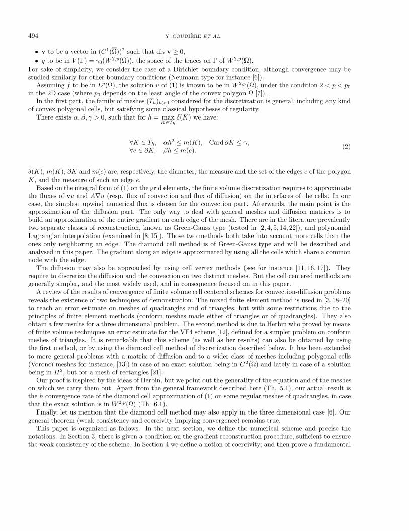
6. Convergence of the diamond cell method on quadrangular meshes

6.1. Hypotheses on the mesh

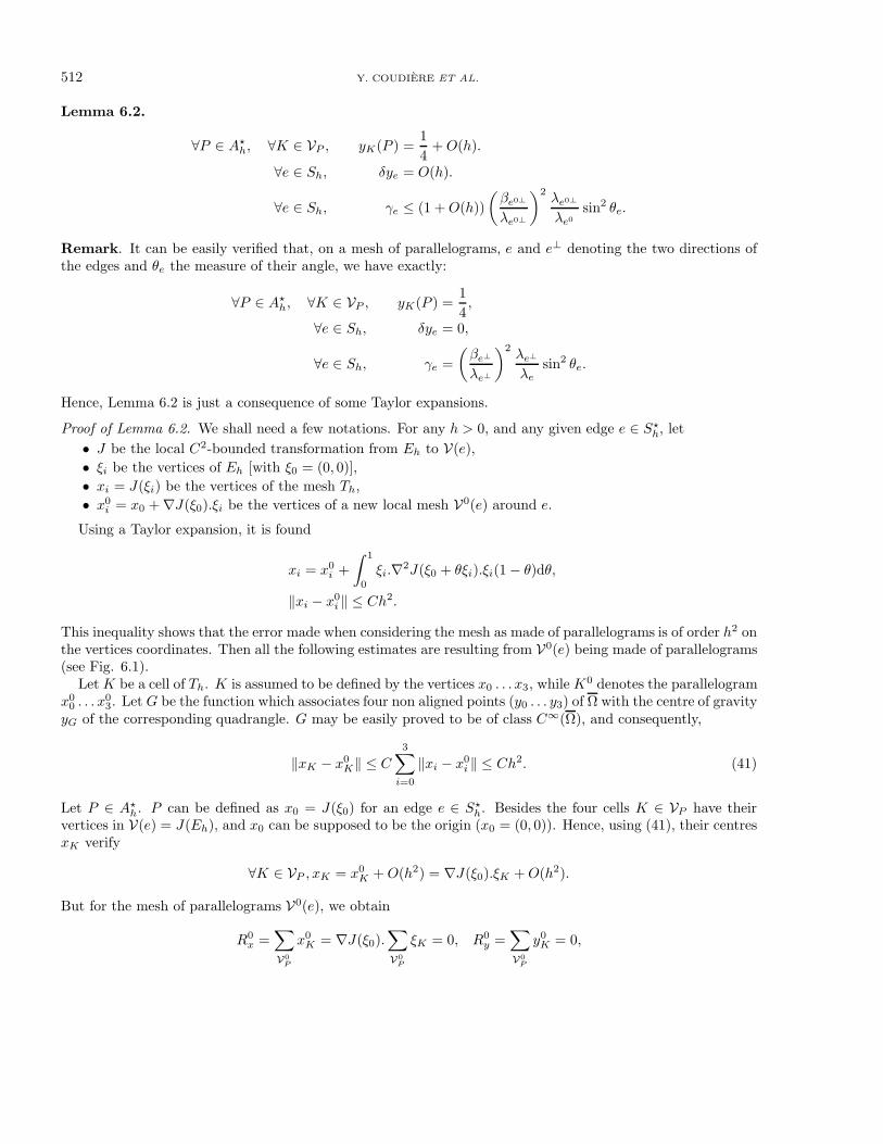
Let Eh be a Cartesian grid made of the vertices Mij = (ih, jh)i=−1...2;j=−1...1 of six squares of length h (seeFig. 6.1) and Qh = [−h, 2h]× [−h, h].

Definition 6.1. The family of meshes (Th)h>0 is said to be admissible if there exists a constant B > 0 suchthat ∀h > 0,∀e ∈ S?h there exists Jh,e ∈ C2(Qh,R2) such that

Jh,e(Eh) = V(e), (32)supx∈Qh

|∇Jh,e(x)|2 ≤ B, (33)

supx∈Qh

|∇2Jh,e(x)|2 ≤ B, (34)

where V(e) denotes the set of the twelve vertices surrounding the edge e of S?h (Eh may be truncated convenientlyif e ∩ Γ is not empty). |.|2 denotes the Euclidian norm.

Remark. If Jh,e is linear (∇Jh,e is constant and ∇2Jh,e = 0) then Jh,e(Qh) is a mesh of six parallelograms.Otherwise, let be LJh,e(x) = Jh,e(x0) +∇Jh,e(x0). (x−x0) the linear tangent application in x0. The differencebetween Jh,e(Qh) (the real mesh) and LJh,e(Qh) (a mesh of parallelogram) is bounded by the derivatives ofJh,e and the characteristic size of the mesh (h). Such meshes are easily proved to verify hypotheses (2).

6.2. Main result

Theorem 6.1. If (Th)h>0 is an admissible family of quadrangular meshes (Def. 6.1), then the finite volumescheme (10), associated with the weights (21), converges to the solution u of (1), and for h small enough,

the discrete problem (10) is well-posed, (35)∃C > 0,∀h > 0, ‖uh − πhu‖1,0 + ‖uh − u‖L2 < Ch. (36)

Proof. Using Theorem 5.1, it just remains to prove the coercivity of the discrete operator Lh. Let us first noticethat, on the edges e of S?h, uN − uS can be naturally spread out into some contributions uE − uW on all theedges f of Ve = VN ∪ VS as follows.


• If e does not intersect the boundary Γ, a short calculation yields

uN − uS = yNW (N)(uNW − uW ) + yNE(N)(uNE − uE)+ ySW (S)(uW − uSW ) + ySE(S)(uE − uSE)+ ((yNE(N) + yE(N)) − (yE(S) + ySE(S))) (uE − uW ).

• If e does intersect the boundary Γ with N = e ∩ Γ, using uN = 0, it is found

uN − uS = −(ySW (S) + yW (S))uW − (ySE(S) + yE(S))uE+ ySW (S)(uW − uSW ) + ySE(S)(uE − uSE)

=12

(0− uW ) +12

(0− uE)

+ ySW (S)(uW − uSW ) + ySE(S)(uE − uSE)

+((

12

+ 0)− (yE(S) + ySE(S))

)(uE − uW ).

So, writing the previous general form prevails with the following notations:

yNW (N) =12

, yNE(N) =12

, yW (N) = 0, yE(N) = 0,uNW = uNE = 0.

• If e does intersect the boundary Γ with e ∩ Γ = S, the same expression remains, just swapping N and S.Let Pe be the set of all the edges f perpendicular to e. The associated weight to such an edge f ∈ Pe is

denoted by yef :

yef = yK(P ) where P = e ∩ f ,e /∈ ∂K while f ∈ ∂K.

As a result, we have∀e ∈ S?h uN − uS = ∆u0

NS + δye(uE − uW )e,where

∆u0NS =

∑f∈Pe

yef (uE − uW )f , (37)

δye = (yNW (N) + yW (N))− (ySW (S) + yW (S)).

At this stage, we note that, with the notations introduced above, QDh (uh) may be written as

∀uh ∈ P0(Th)12QD(uh) =

(Ap⊥h ,ph

)L2 = QD0 (uh) + δQD(uh), (38)

where

QD0 (uh) =∑e∈Sh

(uE − uW

he+βeλe

∆u0NS

m(e)

)uE − uW

heλem(χe),

δQD(uh) =∑e∈S?h

βeλeδye

(uE − uW

he

)2

λem(χe).

Afterwards the proof of coercivity is achieved by using the ideas of Lemma 4.1. The constant γ of condition (25)is performed by collecting on each edge f ∈ Sh the contributions issued of the outspreading of ∆u0

NS [see (37)].It is proved the following estimate (the definition of σe will be precised in the proof).


Lemma 6.1.

∑e∈S?

h

(βeλe

)2(∆u0NS

m(e)

)2

λem(χe) ≤∑f∈Sh

γf

((uE − uW )f

hf

)2

λfm(χf ),

∀f ∈ Sh, γf =∑

e∈Pf∩S?h

σeyef

(βeλe

)2λeλf

hem(f)

·

Proof of Lemma 6.1.βeλe

∆u0NS

m(e)=βeλe

∑f∈Pe

yefhfm(e)

(uE − uW )fhf

·

Using Jensen inequality, we obtain(βeλe

)2 (∆u0NS

m(e)

)2

≤(βeλe

)2

σe∑f∈Pe

yefhfm(e)

((uE − uW )f

hf

)2

,

where

σe =∑f∈Pe

yefhfm(e)

(for e ∈ S?h). (39)

Thus, we have

∑e∈S?h

(βeλe

)2(∆u0NS

m(e)

)2

λem(χe) ≤∑e∈S?h

(βeλe

)2

σe∑f∈Pe

yefhfm(e)

((uE − uW )f

hf

)2

λem(χe).

The desired result is achieved by swapping the two sums:

∑e∈S?h

(βeλe

)2(∆u0NS

m(e)

)2

λem(χe) ≤∑f∈Sh

γf

((uE − uW )f

hf

)2

λfm(χf ),

γf =∑

e∈S?h/f∈Pe

(βeλe

)2

σeyefhfm(e)

λem(χe)λfm(χf )

.

Noticing that e ∈ S?h such that f ∈ Pe ⇔ e ∈ Pf ∩ S?h, γf is simplified to be finally written as

γf =∑

e∈Pf∩S?h

σeyef

(βeλe

)2λeλf

hem(f)

(forf ∈ Sh). (40)

To complete the proof, the main difficulty is to check the condition 0 ≤ γf < 1 for each edge f ∈ Sh.Until this point, we only used the fact that the mesh was structured and we didn’t take into account thegeometric hypothesis (32). . . (34) of Definition 6.1, which ensure the mesh Th to be locally near from a mesh ofparallelograms. This last property is the key ingredient of the following lemma.


Lemma 6.2.

∀P ∈ A?h, ∀K ∈ VP , yK(P ) =14

+O(h).

∀e ∈ Sh, δye = O(h).

∀e ∈ Sh, γe ≤ (1 +O(h))(βe0⊥

λe0⊥

)2λe0⊥

λe0sin2 θe.

Remark. It can be easily verified that, on a mesh of parallelograms, e and e⊥ denoting the two directions ofthe edges and θe the measure of their angle, we have exactly:

∀P ∈ A?h, ∀K ∈ VP , yK(P ) =14,

∀e ∈ Sh, δye = 0,

∀e ∈ Sh, γe =(βe⊥

λe⊥

)2λe⊥

λesin2 θe.

Hence, Lemma 6.2 is just a consequence of some Taylor expansions.

Proof of Lemma 6.2. We shall need a few notations. For any h > 0, and any given edge e ∈ S?h, let• J be the local C2-bounded transformation from Eh to V(e),• ξi be the vertices of Eh [with ξ0 = (0, 0)],• xi = J(ξi) be the vertices of the mesh Th,• x0

i = x0 +∇J(ξ0).ξi be the vertices of a new local mesh V0(e) around e.

Using a Taylor expansion, it is found

xi = x0i +

∫ 1

0

ξi.∇2J(ξ0 + θξi).ξi(1− θ)dθ,

‖xi − x0i ‖ ≤ Ch2.

This inequality shows that the error made when considering the mesh as made of parallelograms is of order h2 onthe vertices coordinates. Then all the following estimates are resulting from V0(e) being made of parallelograms(see Fig. 6.1).

Let K be a cell of Th. K is assumed to be defined by the vertices x0 . . . x3, while K0 denotes the parallelogramx0

0 . . . x03. Let G be the function which associates four non aligned points (y0 . . . y3) of Ω with the centre of gravity

yG of the corresponding quadrangle. G may be easily proved to be of class C∞(Ω), and consequently,

‖xK − x0K‖ ≤ C

3∑i=0

‖xi − x0i ‖ ≤ Ch2. (41)

Let P ∈ A?h. P can be defined as x0 = J(ξ0) for an edge e ∈ S?h. Besides the four cells K ∈ VP have theirvertices in V(e) = J(Eh), and x0 can be supposed to be the origin (x0 = (0, 0)). Hence, using (41), their centresxK verify

∀K ∈ VP , xK = x0K +O(h2) = ∇J(ξ0).ξK +O(h2).

But for the mesh of parallelograms V0(e), we obtain

R0x =

∑V0P

x0K = ∇J(ξ0).

∑V0P

ξK = 0, R0y =

∑V0P

y0K = 0,


and consequently,

Rx = O(h2), Ry = O(h2).

Besides using that ∇J is uniformly bounded, we have

xK = O(h), yK = O(h), Ixx = O(h2), Iyy = O(h2), Ixy = O(h2),

thus,

D = O(h4), λx = O(1), λy = O(1).

Finally it yields

yK(P ) =14

+O(h).

Let f ∈ Sh. The endpoint S of the edge f is supposed to be x0 = J(ξ0). For any edge e ∈ V(f) supposed to beof endpoints x1 and x2, e0 denotes the edge x0

1x02 in the mesh T 0

h of parallelograms.

∣∣m(e)−m(e0)∣∣ =

∣∣‖x1 − x2‖ − ‖x01 − x0

2‖∣∣ ≤ ‖x1 − x0

1‖+ ‖x2 − x02‖ ≤ Ch2.

Let E and W be the centres of the two neighbours of a given edge e ∈ V(f) and E0 and W 0 the correspondingcentres in the local mesh T 0

h of parallelograms. The following estimates are straightforward.

|he − he0 | =∣∣(xW − xE).ne − (x0

W − x0E).ne0

∣∣=

∣∣∣∣‖(xW − xE) ∧ (xN − xS)‖‖xN − xS‖

− ‖(x0W − x0

E) ∧ (x0N − x0

S)‖‖x0

N − x0S‖

∣∣∣∣≤ Ch2.

|αe − αe0 | =∣∣∣∣(xW − xE).(xN − xS)

he‖xN − xS‖− (x0

W − x0E).(x0

N − x0S)

he0‖x0N − x0

S‖

∣∣∣∣ ≤ Ch.Besides, the following properties are clearly observed on the mesh T 0

h .

If e ∈ Pf ∩ S?h,he0

m(f0)= | sin θf |.

If f ∈ S?h, e ∈ Pf ,he0

m(f0)=

| sin θf |(e ∈ S?h)12| sin θf |(e ∈ Γh),

where θf denotes the angle of the parallelograms in the mesh T 0h .

Calculating the matrix Ae in the basis (ne0 , te0) for e ∈ V(f) proceeds by evaluating the formulae of changingbases

Ae0 =[

cos η − sin ηsin η cos η

]Ae

[cosη sin η− sin η cos η

],


where η is the angle between the exact edge e and the approximate one e0; furthermore,

| cos η| =|(x1 − x2).(x0

1 − x02)|

m(e)m(e0)

=‖x0

1 − x02‖2

m(e)2(1 +O(h))+O(h) = 1 +O(h),

| sin η| =‖(x1 − x2) ∧ (x0

1 − x02)‖

m(e)m(e0)

=

∥∥((x1 − x2)− (x01 − x0

2))∧ (x0

1 − x02)∥∥

m(e)m(e0)= O(h).

At last, for f ∈ Sh and e ∈ Pf ∩ S?h, we have

βeλe

=βe0

λe0(1 +O(h)) =

βf0⊥

λf0⊥(1 +O(h)),

λeλf

=λe0

λf0(1 +O(h)) =

λf0⊥

λf0(1 +O(h)),

where f0⊥ denotes the constant direction of the edges e0 for e ∈ Pf .The evaluation of γe and δye proceeds now by collecting all the previous estimates. ∀e ∈ S?h,

σe =∑f∈Pe

yefhfm(e)

=

∑Pe∩S?h

14| sin θe|+

∑Pe∩Γh

12

12| sin θe|

(1 +O(h))

= | sin θe|(1 +O(h)).

The final estimate of γe derives itself from the next remark on the local angles of the parallelograms on twoneighbouring edges.

∀e, f ∈ Sh/e ∩ f 6= ∅, |θe| = |(e0, e0⊥)| = |(e, f)|(1 +O(h)),

|θf | = |( f0, f0⊥)| = |(f, e)|(1 +O(h)),

and so,∀e ∈ S?h, ∀f ∈ Pe, |θe| = |θf |(1 +O(h)) and σe = | sin θf |(1 +O(h)).

Afterwards, γf and δye are performed easily:

∀e ∈ S?h, δye = O(h), (42)

∀f ∈ Sh, γf ≤(βf0⊥

λf0⊥

)2 λf0⊥

λf0sin2 θf (1 +O(h)). (43)

End of the proof of Theorem 6.1. The coercivity is achieved by substituting (42, 43) in the expression of δQDand in Lemma 4.1. The remainder δQD is obviously estimated.

|δQD| ≤∑e∈S?h

|βeδye|(uE − uW

he

)2

m(χe) ≤ βmaxO(h)‖uh‖21,0

(since βe = µe − αeλe is clearly uniformly bounded).


Furthermore, Lemma 4.1 provides the following estimate of QD0 .

QD0 (uh) ≥ 2 infh>0,e∈Sh

λe(1− γe)2

‖uh‖21,0.

Finally a more precise estimate of λe(1− γe) brings out the final constant of coercivity.

λe(1− γe) ≥ λe0

(1−

(βe0⊥

λe0⊥

)2λe0⊥

λe0sin2 θe

)(1 +O(h))

=(λe0λe0⊥ − β2

e0⊥ sin2 θe) 1λe0⊥

(1 +O(h))

=(λe0λe0⊥ − (µe0⊥ sin θe + λe0⊥ cos θe)

2) 1λe0⊥

(1 +O(h)),

because βe0⊥ = µe0⊥ − αe0⊥λe0⊥ and αe0⊥ = −cotanθe (see Fig. 6.1).Using the previous changing bases formulae from the basis of e0⊥ to the basis of e0, between which the angle

is actually θe yieldsλe0 = λe0⊥ cos2 θe + νe0⊥ sin2 θe + 2µe0⊥ cos θe sin θe,

and consequently,

λe(1− γe) =(νe0⊥λe0⊥ − µ2

e0⊥)

sin2 θe1

λe0⊥(1 +O(h))

=detAe0⊥ sin2 θe

λe0⊥(1 +O(h))

≥ λmin sin2 θmin(1 +O(h)),

where θmin denotes the smallest angle in the cells K of the (Th)h>0. This completes the proof.

References

[1] R.A. Adams, Sobolev Spaces. Academic Press, New-York (1975).[2] M. Aftosmis, D. Gaitonde and T. Sean Tavares, On the accuracy, stability and monotonicity of various reconstruction algorithms

for unstructured meshes. AIAA paper No. 94-0415 (1994).[3] J. Baranger, J.F. Maitre and F. Oudin, Connection between finite volume and mixed finite element methods. RAIRO Model.

Math. Anal. Num. 30 (1996) 445–465.[4] W.J. Coirier, An Adaptatively-Refined, Cartesian, Cell-based Scheme for the Euler and Navier-Stokes Equations. Ph.D. thesis,

Michigan University, NASA Lewis Research Center, USA (1994).[5] W.J. Coirier and K.G. Powell, A Cartesian, cell-based approach for adaptative-refined solutions of the Euler and Navier-Stokes

equations. AIAA (1995).[6] Y. Coudiere, Analyse de schemas volumes finis sur maillages non structures pour des problemes linaires hyperboliques et

elliptiques. Ph.D. thesis, Paul Sabatier University, France (1998).[7] M. Dauge, Elliptic Boundary Value Problems in Corner Domains. Lect. Notes Math. 1341, Springer Verlag, Berlin-New York

(1988).[8] F. Dubois, Interpolation de Lagrange et volumes finis. Une technique nouvelle pour calculer le gradient d’une fonction sur les

faces d’un maillage non structure. Technical report, Aerospatiale (1992).[9] I. Faille, A control volume method to solve an elliptic equation on a 2d irregular meshing. Comput. Methods. Appl. Mech.

Engrg. 100 (1992) 275–290.[10] T. Gallouet, An introduction to finite volume methods. Technical report, Cours CEA/EDF/INRIA (1992).[11] W. Guo and M. Stynes, An analysis of a cell-vertex finite volume method for a parabolic convection-diffusion problem. Math.

Comp. 66 (1997) 105–124.[12] R. Herbin, An error estimate for a finite volume scheme for a diffusion-convection problem on a triangular mesh. Numerical

Method for Partial Differential Equations 11 (1994) 165–173.


[13] R. Herbin, Finite volume methods for diffusion convection equations on general meshes, in Finite Volumes for ComplexApplications, Hermes (1996) 153–160.

[14] F. Jacon and D. Knight, A Navier-Stokes algorithm for turbulent flows using an unstructured grid and flux difference splitting.AIAA paper No. 94-2292 (1994).

[15] C.R. Mitchell and R.W. Walters, K-exect reconstruction for the Navier-Stokes equations on arbitrary grids. AIAA (1993).[16] K.W. Morton and E. Suli, Finite volume methods and their analysis. IMA J. Numer. Anal. 11 (1991) 241–260.[17] E. Suli, Convergence of finite volume schemes for Poisson’s equation on nonuniform meshes. SIAM J. Numer. Anal. 28 (1991)

1419–1430.[18] J.-M. Thomas and D. Trujillo, Analysis of finite volumes methods. Technical Report 95/19, CNRS, URA 1204 (1995).[19] J.-M. Thomas and D. Trujillo, Convergence of finite volumes methods. Technical Report 95/20, CNRS, URA 1204 (1995).[20] D. Trujillo, Couplage espace-temps de schemas numeriques en simulation de reservoir. Ph.D. thesis, University of Pau et pays

de l’Adour (1994).[21] S. Verdiere and M.H. Vignal, Numerical and theoretical study of a dual mesh method using finite volume schemes for two

phase flow problems in porous media. Numer. Math. 80 (1998) 601–639.[22] P. Villedieu, Une methode de volumes finis sur maillages non-structures quelconques pour l’equation de convection diffusion.

Technical Report 1-3550.00-DERI, ONERA (1996).

Documents

Convergence rate of a finite volume scheme for a two dimensional convection-diffusion … · Mathematical Modelling and Numerical Analysis M2AN, Vol. 33, No 3, 1999, p. 493{516 Mod