Convergence of Government Bond Yields in the Euro … · Convergence of Government Bond Yields in the Euro Zone: The Role of Policy Harmonization by ... Florian Pelgrin, James Powell,

Bank of Canada Banque du Canada

Working Paper 2004-23 / Document de travail 2004-23

Convergence of Government Bond Yields in theEuro Zone: The Role of Policy Harmonization

by

Denise Côté and Christopher Graham

ISSN 1192-5434

Printed in Canada on recycled paper

Bank of Canada Working Paper 2004-23

June 2004

Convergence of Government Bond Yields in theEuro Zone: The Role of Policy Harmonization

by

Denise Côté and Christopher Graham

International DepartmentBank of Canada

Ottawa, Ontario, Canada K1A [email protected]

[email protected]

The views expressed in this paper are those of the authors.No responsibility for them should be attributed to the Bank of Canada.

. . . . 2

. . . . 3

. .

. . . . 9

. . . 12

.

. . . 14

. . . 16

19

. 20

1

. 23

.

. . 32

. . .

iii

Contents

Acknowledgements. . . . . . . . . . . . . . . . . . . . . . . . . . . . . . . . . . . . . . . . . . . . . . . . . . . . . . . . . . . . ivAbstract . . . . . . . . . . . . . . . . . . . . . . . . . . . . . . . . . . . . . . . . . . . . . . . . . . . . . . . . . . . . . . . . . . . . . . vRésumé . . . . . . . . . . . . . . . . . . . . . . . . . . . . . . . . . . . . . . . . . . . . . . . . . . . . . . . . . . . . . . . . . . . . . vi

1. Introduction . . . . . . . . . . . . . . . . . . . . . . . . . . . . . . . . . . . . . . . . . . . . . . . . . . . . . . . . . . . . . . 1

2. Institutional Background and Stylized Facts . . . . . . . . . . . . . . . . . . . . . . . . . . . . . . . . .

2.1 Institutional background . . . . . . . . . . . . . . . . . . . . . . . . . . . . . . . . . . . . . . . . . . . .

2.2 Stylized facts. . . . . . . . . . . . . . . . . . . . . . . . . . . . . . . . . . . . . . . . . . . . . . . . . . . . .. . 4

3. Literature Review. . . . . . . . . . . . . . . . . . . . . . . . . . . . . . . . . . . . . . . . . . . . . . . . . . . . . .. . . . 7

3.1 Government fiscal position. . . . . . . . . . . . . . . . . . . . . . . . . . . . . . . . . . . . . . . . . .

3.2 Expected inflation . . . . . . . . . . . . . . . . . . . . . . . . . . . . . . . . . . . . . . . . . . . . . . . . .

4. Empirical Analysis. . . . . . . . . . . . . . . . . . . . . . . . . . . . . . . . . . . . . . . . . . . . . . . . . . . . . . . 13

4.1 Country-by-country analysis. . . . . . . . . . . . . . . . . . . . . . . . . . . . . . . . . . . . . . . . .

4.2 Panel estimations and error-correction models. . . . . . . . . . . . . . . . . . . . . . . . . . .

4.2.1 Standard panel estimations of the long-run parameters. . . . . . . . . . . . . . . . . 16

4.2.2 Error-correction models. . . . . . . . . . . . . . . . . . . . . . . . . . . . . . . . . . . . . . . . .

4.2.3 Sensitivity analysis . . . . . . . . . . . . . . . . . . . . . . . . . . . . . . . . . . . . . . . . . . . .

4.2.4 Further results of the long-run analysis. . . . . . . . . . . . . . . . . . . . . . . . . . . . . 2

4.2.5 Empirical interpretation of the trend 10-year government bond yield. . . . . . 22

4.2.6 Currency risk . . . . . . . . . . . . . . . . . . . . . . . . . . . . . . . . . . . . . . . . . . . . . . . .

5. Conclusions . . . . . . . . . . . . . . . . . . . . . . . . . . . . . . . . . . . . . . . . . . . . . . . . . . . . . . . . . . . . . 25

Bibliography . . . . . . . . . . . . . . . . . . . . . . . . . . . . . . . . . . . . . . . . . . . . . . . . . . . . . . . . . . . . . . . . . 28

Appendix A: Data Description . . . . . . . . . . . . . . . . . . . . . . . . . . . . . . . . . . . . . . . . . . . . . . . . . . 31

Appendix B: Timeline for Economic and Monetary Union . . . . . . . . . . . . . . . . . . . . . . . . . . .

Appendix C: Tables and Figures. . . . . . . . . . . . . . . . . . . . . . . . . . . . . . . . . . . . . . . . . . . . . . . 36

aryl

ri for

Teske,

are

t the

inance

f the

for his

iv

Acknowledgements

We would like to thank Jocelyn Jacob, Peter Hann, Michael King, Robert Lafrance, D

Merrett, Graydon Paulin, Florian Pelgrin, James Powell, Eric Santor, and Larry Schemb

helpful suggestions and discussions. We would like to thank our research assistants, Joan

Sylvie Malette, and Danielle Henri, for providing help in constructing the database. We

grateful for the comments received at a seminar at the Bank of England in April 2004, a

European Central Bank, and at the 3rd Annual Meeting of the European Economics and F

Society, University of Gdansk, Poland, in May 2004 and at the 38th Annual Meetings o

Canadian Economics Association in June 2004. We are also thankful to Glen Keenleyside

excellent work in editing this document.

in line

ry and

nion

have

ne.

n the

n the

-term

f the

imilar

s not

ludes

rway,

dually

ingle

grated

cross

e euro

the

v

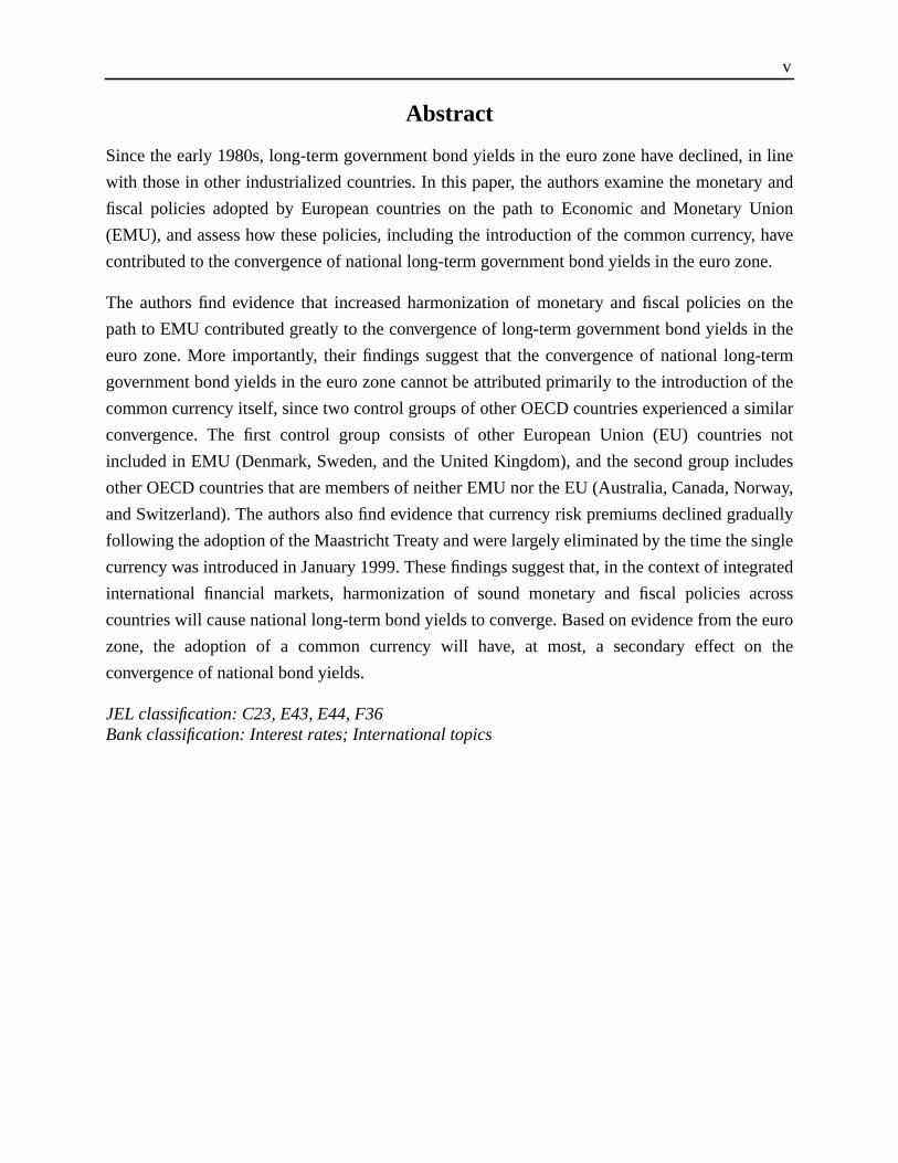
Abstract

Since the early 1980s, long-term government bond yields in the euro zone have declined,

with those in other industrialized countries. In this paper, the authors examine the moneta

fiscal policies adopted by European countries on the path to Economic and Monetary U

(EMU), and assess how these policies, including the introduction of the common currency,

contributed to the convergence of national long-term government bond yields in the euro zo

The authors find evidence that increased harmonization of monetary and fiscal policies o

path to EMU contributed greatly to the convergence of long-term government bond yields i

euro zone. More importantly, their findings suggest that the convergence of national long

government bond yields in the euro zone cannot be attributed primarily to the introduction o

common currency itself, since two control groups of other OECD countries experienced a s

convergence. The first control group consists of other European Union (EU) countrie

included in EMU (Denmark, Sweden, and the United Kingdom), and the second group inc

other OECD countries that are members of neither EMU nor the EU (Australia, Canada, No

and Switzerland). The authors also find evidence that currency risk premiums declined gra

following the adoption of the Maastricht Treaty and were largely eliminated by the time the s

currency was introduced in January 1999. These findings suggest that, in the context of inte

international financial markets, harmonization of sound monetary and fiscal policies a

countries will cause national long-term bond yields to converge. Based on evidence from th

zone, the adoption of a common currency will have, at most, a secondary effect on

convergence of national bond yields.

JEL classification: C23, E43, E44, F36Bank classification: Interest rates; International topics

e euro

s pays

étaires

M) et

ns la

ne euro.

litiques

rgence.

ue n’a

deux

re. Le

rtie de

sé de

voir

nent à

Traité

unique,

ires et

’échelle

terme.

out au

vi

Résumé

Depuis le début des années 1980, les rendements des obligations d’État dans la zon

affichent une tendance à la baisse, laquelle a également été observée dans d’autre

industrialisés. Dans cette étude, les auteurs examinent les politiques monétaires et budg

qu’ont adoptées les pays européens en voie d’intégrer l’Union économique et monétaire (UE

évaluent le rôle joué par ces politiques, y compris l’introduction de la monnaie unique, da

convergence des rendements des obligations à long terme émises par les membres de la zo

Les résultats obtenus par les auteurs indiquent que la poursuite de l’harmonisation des po

monétaires et budgétaires des candidats à l’UEM a favorisé considérablement cette conve

Plus important encore, ces résultats semblent montrer que l’introduction de la monnaie uniq

pas joué un rôle primordial à cet égard, les rendements des obligations à long terme de

groupes témoins formés d’autres pays de l’OCDE ayant connu une convergence similai

premier groupe comprend les pays membres de l’Union européenne qui ne font pas pa

l’union monétaire, soit le Danemark, la Suède et le Royaume-Uni. Le second est compo

quatre membres de l’OCDE qui ne font partie ni de l’UEM ni de l’Union européenne, à sa

l’Australie, le Canada, la Norvège et la Suisse. Par ailleurs, certaines observations don

penser que les primes de risque de change ont diminué graduellement après l’adoption du

de Maastricht et avaient en grande partie disparu au moment du lancement de la monnaie

en janvier 1999. Ces résultats portent à croire que l’harmonisation de politiques monéta

budgétaires saines entre les pays, dans le contexte de marchés financiers intégrés à l

internationale, entraîne une convergence des rendements des obligations d’État à long

L’expérience vécue dans la zone euro montre que l’adoption d’une monnaie unique aura, t

plus, un effet secondaire à cet égard.

Classification JEL : C23, E43, E44, F36Classification de la Banque : Taux d’intérêt; Questions internationales

1

in line

uced

that of

s to a

debt

turn,

euro-

, and

terest

this

r the

ry and

nion

have

ne.

ues to

ool of

riod.

ark,

ECD

either

nts:

eneral

ation.

large

tion).

1. Introduction

Since the early 1980s, long-term government bond yields in the euro zone have declined,

with those in other industrialized countries. In fact, by the time the euro currency was introd

in 1999, long-term government bond yields across the euro zone had largely converged to

Germany (the euro zone’s largest economy). In general, the convergence of national yield

stable level with reduced risk aids the overall economy, by allowing cheaper access to

financing with less uncertainty regarding the value of such funds over time. This, in

stimulates investment and output within converging countries. The recent expansion of the

zone bond market is one beneficial outcome of this process (Hartmann, Maddaloni

Manganelli 2003). Given the stabilizing effect that convergence to stable and predictable in

rates has on the financial system, it is important to identify the factors that can bring

convergence about and maintain it over the long term.

Statements by the European Central Bank (2003) give one possible explanation fo

convergence of yields observed in the euro zone:

In the run-up to Stage Three of Economic and Monetary Union, which started on 1January 1999, there was a significant convergence in the long-term governmentbond yields of those countries which subsequently adopted the euro. Thisconvergence was driven by the anticipation of the introduction of the euro and thecorresponding elimination of intra-euro area exchange rate risk.

In an effort to investigate the convergence of national bond yields, we examine the moneta

fiscal policies adopted by European countries on the path to Economic and Monetary U

(EMU), and assess how these policies, including the introduction of the common currency,

contributed to the convergence of national long-term government bond yields in the euro zo

To shed some light on this issue, our study uses cointegration and panel estimation techniq

analyze a set of long-term determinants of 10-year nominal government bond yields for a p

EMU countries and two control groups of other OECD countries over the 1980 to 2002 pe

The first control group consists of three European Union (EU) countries (EU3: Denm

Sweden, and the United Kingdom) not included in EMU, and the second includes other O

countries (OECD4: Australia, Canada, Norway, and Switzerland) that are members of n

EMU nor the EU. In our empirical work, we consider the following set of long-term determina

general government fiscal balance as a share of nominal GDP; the stock of accumulated g

government debt as a share of nominal GDP, to account for country risk; and expected infl

We also include a measure of the world real long-term bond yield, since developments in

countries influence real long-term yields in smaller countries (small open-economy assump

2

ath to

euro

our

euro

our

ilar

n of

uced

ancial

tional

n of a

bond

the

iven

ajor

ylized

bond

ental

long-

ental

ion is

d to the

g the

arch.

, and,

omic

the

Our results indicate that increased harmonization of monetary and fiscal policies on the p

EMU contributed greatly to the convergence of long-term government bond yields in the

zone, by prompting the convergence of their long-run determinants. More importantly,

findings suggest that the convergence of national long-term government bond yields in the

zone cannot be attributed primarily to the introduction of the common currency itself, since

two control groups of other OECD countries (EU3 and OECD4) experienced a sim

convergence.

We also find evidence that currency risk premiums declined gradually following the adoptio

the Maastricht Treaty and were largely eliminated by the time the single currency was introd

in January 1999. These findings suggest that, in the context of integrated international fin

markets, harmonization of sound monetary and fiscal policies across countries will cause na

long-term bond yields to converge. Based on evidence from the euro zone, the adoptio

common currency will have, at most, a secondary effect on the convergence of national

yields. With regards to the EU3 and OECD4, however, the policy commitment inherent in

framework for the adoption of the euro currency (i.e., the Maastricht criteria) may have g

additional credibility to national euro-zone monetary and fiscal policies.

This paper is organized as follows. Section 2 provides institutional background on the m

economic policies adopted by European countries on the path to EMU, and reviews the st

facts on how these policies have likely contributed to the convergence of the euro-zone

market. Section 3 surveys the existing theoretical and empirical literature on the fundam

determinants of long-term interest rates. Section 4 provides new empirical evidence on the

run relationship between the 10-year nominal government bond yield and its fundam

determinants on a country-by-country basis, and using panel estimation. Empirical informat

then used to assess how increased harmonization of monetary and fiscal policies contribute

convergence of long-term government bond yields across euro-zone countries by drivin

convergence of their long-run determinants. Section 5 concludes and suggests future rese

2. Institutional Background and Stylized Facts

This section provides some institutional background regarding the path towards the EU

subsequently, the common currency. We then review the stylized facts on how key econ

policies adopted by the various countries in the lead up to EMU likely contributed to

convergence of the euro-zone bond market.

3

EMU

pean

pean

es of

eaty

ere to

rrency

were

would

rates

re than

terms

points

for at

nging

f

, Italy,

embersjecteddum inas not

stonia,pt the

2.1 Institutional background

This section summarizes the institutional background. Appendix B provides a detailed

timeline.

EMU was built on over 40 years of concerted economic integration between western Euro

nations. By the late 1980s, the majority of this integration had taken place. The Euro

Community, as it was then known, had grown to 12 members, including the recent inducte

Greece (1981), Spain (1986), and Portugal (1987).

The EU as we know it today was born out of the Maastricht Treaty in 1993.1 Besides enacting a

common foreign and security policy, and dealing with EU-level matters of justice, this tr

specified the three steps required for EMU to take place: by the end of 1993, capital flows w

be completely freed within the EU; by 1999, member states preparing to adopt the euro cu

upon its launch had to satisfy a set of convergence criteria by which major economic policies

coordinated across nations; effective at the beginning of 1999, the European Central Bank

be established, along with the official euro currency for which member-country conversion

were irrevocably set. The Maastricht Treaty convergence criteria were as follows:

• the ratio of general government deficit to GDP must not exceed 3 per cent

• the ratio of gross general government debt to GDP must not exceed 60 per cent

• the average inflation rate over the year before assessment must not exceed by mo

1.5 percentage points the average of the three best performing member states in

of price stability

• the long-term nominal interest rate must not exceed by more than 2 percentage

the average of the three best performing member states in terms of price stability

• the exchange rate mechanism (ERM) must be respected without severe tensions

least the last two years before assessment

In 1995, three new members were admitted to the EU (Austria, Finland, and Sweden), bri

the total number of member states to 15.2,3 At the launch of the euro in 1999, EMU consisted o

1. The original member states of the EU were Belgium, Denmark, France, Germany, Greece, IrelandLuxembourg, the Netherlands, Portugal, Spain, and the United Kingdom.

2. Norway and Switzerland, while remaining members of the European Free Trade Association, are not mof the EU. Norway has applied twice for accession. The first application was submitted in 1967 but was rein a national referendum in 1972. In 1992, Norway again applied for membership, but a second referen1994 failed to pass. Switzerland applied for membership in 1992 and maintains an open invitation, but hactively pursued membership.

3. Ten new European countries joined the EU on 1 May 2004: Poland, Hungary, the Czech Republic, ELatvia, Lithuania, Slovakia, Slovenia, Cyprus, and Malta. New members are required to eventually adoeuro and will, thus, have to satisfy the convergence criteria, including the current version of the ERM.

4

om,

euro

going

Pact

ntly,

ty in

the

to an

read of

80 to

1983

rgence

), the

first

. The

e, as

as aventualow astonia,

g new

r cent

ture a, theper cent

on 3.1)en dataple in

11 of the 15 EU countries; those that did not participate in EMU were the United Kingd

Sweden, Denmark, and Greece (Greece later joined in 2001).4 By the beginning of 2002, all

former national currencies (also known as “legacy” currencies) were phased out and the

became the sole legal currency in EMU member states.

Now that monetary integration has been realized in much of western Europe, the on

challenge is for all EU member countries to continuously meet the Stability and Growth

(primarily, the first two conditions of the Maastricht Treaty convergence criteria). Curre

several members of EMU (including Germany, France, and Italy) are experiencing difficul

maintaining a deficit-to-GDP ratio below the 3 per cent limit and a debt-to-GDP ratio below

60 per cent maximum.5

2.2 Stylized facts

Figures 1 and 2 show that euro-zone long-term government bond yields have converged

extraordinary degree over the course of the last 20 years. Figure 3 shows the average sp

long-term government bond yields in eight countries versus the German yield over the 19

2003 period.6 This spread declined from a high of 646 basis points in the second quarter of

to a low of 12 basis points in the same quarter of 1998, which suggests a substantial conve

in national yields over this period. Throughout the remainder of our sample (1999 to 2002

average spread was about 21 basis points.7

A gradual downward trend is visible in Figure 3, accentuated by three steep drops: the

occurring in the mid-1980s, the second in the early 1990s, and the third in the mid-1990s

path of major economic policy variables, as well as changes in the institutional structur

discussed in section 2.1, likely contributed to this convergence.

4. In sync with the second stage of EMU, 1999 marked the introduction of ERMII, which replaced the ERMvoluntary means for non-EMU members of the EU to reduce exchange rate fluctuations and prepare for eadoption of the euro. Currently, Denmark is the only nation participating in ERMII and has elected to foll4.5 per cent band around the euro, as opposed to the minimum requirement of a 30 per cent band. ELithuania, Slovenia, and Cyprus are expected to apply in 2004 for entrance into ERMII, with the remainincentral and eastern European EU members to follow.

5. Italy is a special case, in that it was admitted to EMU with a debt-to-GDP limit far exceeding the 60 pelimit, on the condition that this level be reduced over time.

6. Figure 3 and all tables in this paper report empirical results for the nine euro zone countries that feacomplete dataset available from 1980 to 2002 (Austria, Belgium, Finland, France, Germany, ItalyNetherlands, Portugal, and Spain), unless otherwise noted. Together, these countries made up about 96of U.S.-dollar euro-zone GDP in 2002. Although data are available from 1977, some studies (see sectisuggest (and our findings concur) that the relationship between fiscal variables and yields is unclear whfrom the 1970s are included. Hence, we follow the convention of existing literature and begin our sam1980.

7. As of 2003Q4, the average spread was about 7 basis points.

5

ently

ould

l side,

ion of

d the

rium

-zone

lower

-term

nce in

980s

its

oods

eneral

rriers

mann,

used

in the

an to

nt in

s of

satisfy

gence

ed by

tween

two

onds

reaty

period

of past

ver the

As Figures 4 and 5 illustrate, monetary policy in the future euro-zone countries independ

achieved a notable disinflation beginning in the early 1980s.8 To the extent that movements in

inflation are reflected in nominal interest rates, national 10-year government bond yields w

have declined as well, contributing to their convergence across countries. On the fisca

general government balance and debt levels also began to improve following the introduct

the Maastricht Treaty (Figures 6 to 9). By reducing the net supply of issued bonds an

likelihood of default, such progress in fiscal positions could be expected to lower the equilib

yield and the risk premium attached to long-term government bond yields. Indeed, euro

national sovereign credit ratings have, on the whole, improved over this period, reflecting

default risk.9 Thus, fiscal policy also appears to have contributed to the convergence of long

government bond yields across the euro-zone countries.

Regulatory changes, as discussed earlier, mark the more rapid periods of converge

government bond yields. For instance, in Figure 3, the decline during the mid- to late 1

coincides with the signing of the Single European Act (SEA) in February of 1986, and

entrance into force the following July. The goals of this act—to achieve a single market for g

and services, labour, and capital within five years—marked a renewed push towards g

economic and financial integration between members of the EU. In turn, this reduction in ba

between countries aided convergence of financial markets, including the bond market (Hart

Maddaloni, and Manganelli 2003). Also in Figure 3, an upward swing is visible in 1992, ca

by the September ERM crisis. Soon after, a strong push was made towards convergence

lead up to the Maastricht Treaty’s entrance into force in November of 1993. Investors beg

take account of the low inflation, improved fiscal position, and lower risk premiums inhere

the convergence criteria. The mid-1990s were, however, an uncertain period in term

compliance with the Maastricht Treaty. Nonetheless, as the national governments acted to

the necessary criteria, relative long-term yields entered one final period of rapid conver

during the second half of the 1990s.

The convergence of long-term government bond yields since 1980 is also characteriz

increased co-movement between national yields. Table 1 illustrates the rise in correlation be

the individual national long-term government bond yields and the German yields over the

halves of our sample. Notably, dividing our sample in half around 1991/1992 also corresp

closely to the signing of the Maastricht Treaty (draft signed 10 December 1991 and final t

signed 7 February 1992). On average, the correlation has increased from 0.69 over the

8. The measure of expected inflation shown in Figures 4 and 5 is simply a geometrically declining averageyear-over-year inflation values.

9. For instance, Moody’s has increased their rating for Finland, Greece, Ireland, Italy, Portugal, and Spain operiod 1993 to 2002 (see Moody’s 2003).

6

lation

high

t both

ect to

etary

yields.

each

(as a

mplete

nt

sitive

n is

nger

plains

980s

.

g-term

sitive

yield,

t this

of our

by the

lance

GDP to

ence

tively

egan in

eds andmentd in the

1980 to 1991 to 0.97 over 1991 to 2002, with all countries showing an increase in corre

between the two periods. Interestingly, Austria and the Netherlands maintained very

correlations with the German yield throughout our entire sample due, in part, to the fact tha

countries had pegged their currencies to the Deutsche Mark and were effectively subj

German monetary policy.10

Simple correlations also help provide preliminary evidence of how the harmonization of mon

and fiscal policies contributed to the convergence of euro zone long-term government bond

Tables 2 and 3 report relevant correlation statistics between the long-term bond yield of

country and corresponding data for expected inflation, general government balance

percentage of GDP), and general government debt (as a percentage of GDP) over our co

sample and the two halves of our sample, respectively.11 Figures 4 through 9 depict these releva

variables for the euro zone.

The Fisher principle suggests that expected inflation should have a one-for-one po

relationship with the long-term nominal yield. Indeed, over our sample, expected inflatio

strongly positively correlated with the long-term bond yield. Moreover, this correlation is stro

in the first half of the sample (0.810 versus 0.653), which suggests that expected inflation ex

more of the movement in the nominal long-term yield during the general disinflation of the 1

than during the period of relatively low and stable inflation in the second half of the sample

The correlation between the general government balance as a percentage of GDP and lon

bond yields is generally negative over our sample, lending credence to the theory that po

balances (i.e., budgetary surpluses) effectively reduce the supply of bonds, and thereby the

as well as the perceived default risk on sovereign debt. Although not all countries exhibi

negative relationship over the 1980 to 1991 period, the opposite is true in the second half

sample. The general increase in government balances (i.e., reduced deficits), as required

Maastricht Treaty, led all countries to show a negative relationship between their fiscal ba

and long-term yield.

Relatedly, one may also expect changes in the level of government debt as a percentage of

indicate an altered level of default risk, especially in light of the Maastricht Treaty converg

criteria. In the long run this should hold, however. Over our sample, government debt is nega

10. Austria’s currency was pegged to the Deutsche Mark starting in 1974, whereas the Netherlands’ peg b1983. Both currencies continued to trade tightly with the Deutsche Mark while in the ERM.

11. General government balance and debt data are thought to capture more fully overall external financing nedefault risk for a given long-term sovereign debt instrument, since any default by lower levels of govern(e.g., state, local) may ultimately be financed by the central government. These measures are also usedefinition of the Stability and Growth Pact.

7

(see

licies

in the

re on

nd for,

e)

apital

holds

nds.

from

cific

the

m by

pends

es and

nterest

made

d in the

effects

rdian

are far-

etweeneasedsimilarnce in

. Thisopen

correlated with the long-term yield, which suggests a need for further empirical investigation

section 4).12

Overall, preliminary evidence indicates that increased harmonization of macroeconomic po

on the path to EMU helped promote the convergence of long-term government bond yields

euro zone. In the following section, we survey the existing theoretical and empirical literatu

the fundamental determinants of long-term interest rates.

3. Literature Review

Interest rates on financial assets like bonds are determined in credit markets by the dema

and supply of, loanable funds.13 Ultimately, the propensity to save (rate of time preferenc

determines the supply of loanable funds (or demand for bonds), and the productivity of c

determines the demand for funds (or the supply of bonds). In the former case, house

optimize their intertemporal consumption-saving decisions, thus influencing the supply of fu

In the latter case, the productivity of capital or perceived rate of return on capital results

optimizing decisions of firms, which in turn determines the demand for funds. In the spe

instance of the government bond market, however, the supply of bonds results from

government’s fiscal position.14

Governments finance their spending/investment by taxing consumers or borrowing from the

issuing debt. The amount of debt issuance (i.e., the demand for funds or supply of bonds) de

on the government’s external financing needs; i.e., the difference between their expenditur

tax revenues. Through bonds, consumers hold a claim on government debt. The effect on i

rates of a change in government fiscal position depends, however, on the assumption

regarding the consumption–savings decisions of households. Several views are documente

economic literature, but there are three main schools of thought concerning the economic

of government fiscal positions (Bernheim 1989): the neoclassical, Keynesian, and Rica

paradigms. The central issues among these schools of thought are whether consumers

sighted and whether they consider government bonds as wealth.

12. For many countries (especially after 1992), dynamic correlations reveal a strong positive relationship bthe long-term yield today and government debt eight to twenty quarters in the future. Likewise, an incrnegative relationship is shown between the long-term yield today and the government balance at ahorizon. These facts imply an important role for current expectations of the future level of debt and baladetermining the current long-term government bond yield.

13. The equilibrium interest rate is the price that equilibrates saving and investment in the economyequilibrium corresponds to an economy operating at full capacity with stable inflation. For smalleconomies, this also requires that the exchange rate be in equilibrium.

14. This does not preclude public spending on productive investment projects.

8

ed and

). In

ilities

urrent

mand

y, the

on net

tment

ined.

iture. It

rk, an

regate

ational

gs (IS)

ng the

the

effect

that

re be

bsence

te-

truistic

astic

by the

not be

fersOtheruests,

of timeficits/

In the neoclassical paradigm (Diamond 1965), it is assumed that consumers are far-sight

plan their consumption profile over their entire lifetime (i.e., individuals have finite lifespans

this framework, an increase in the government’s budget deficit, for example, shifts tax liab

onto future generations, and therefore raises the lifetime consumption of individuals of the c

generation. In a closed economy with full employment, the stimulus to aggregate de

produces higher interest rates and crowds out private investment. In an open econom

widened budget deficit has, to some degree, an impact on the exchange rate and therefore

exports. In a small open economy (that takes the world interest rate as given), all the adjus

occurs through net exports.

In the Keynesian framework, a large proportion of consumers are myopic or liquidity-constra

They ignore future tax increases that are necessary to finance a rise in government expend

is also assumed that the economy begins in a position of underemployment. In this framewo

increase in the government budget deficit leads to a proportionately large increase in agg

demand and nominal income. Because of this increase in nominal GDP, aggregate n

savings may or may not decline, so the effect on interest rates is unclear.

In both paradigms, an exogenous change in the fiscal position shifts the investment–savin

curve, since economic agents consider government bonds to be wealth, thereby affecti

interest rate. While the full-employment assumption and self-equilibrating forces push

economy back to equilibrium in the neoclassical model, a fiscal shock may have permanent

in the Keynesian framework if the shock occurs in a position of underemployment.

In the modern Ricardian paradigm (Barro 1974), rational and far-sighted individuals realize

government spending must be paid for either now or later. Government dissaving will therefo

offset fully by increased household saving, in anticipation of future tax liabilities.15 Ricardian

equivalence, however, is obtained under a number of stringent assumptions, including the a

of liquidity constraints and infinite foresight. Moreover, to obtain infinite foresight with fini

lived agents, it must be assumed that successive generations are linked by a purely al

bequest motive, with the implication that consumption is determined as a function of dyn

resources (the total resources of an individual and all of their descendants), unaffected

timing of taxes (Bernheim 1987, 1989).16

15. An increase in the deficit that reflects additional public spending on productive investment projects wouldexpected to require further taxes later, however, and thus should not elicit a private saving response.

16. This dynastic view of the family assumes that each family is an infinitely lived unit; it therefore difconsiderably from the neoclassical model and the life-cycle model, which assumes finite lifetimes.intertemporal models combine the infinite horizon approach with a constant probability of death, no beqand a positive birth rate, thereby introducing a wedge in equilibrium between rates of interest and ratespreference (Yaari 1965, Blanchard 1985, Buiter 1988). These latter models imply that government desurpluses are largely, but not completely, offset by private saving.

9

s on

wing

ts of

e likely

e. We

in our

w in

in the

other

uiter

85).

e by

rdian

t each

ing of

being

theless,

nds),

et by

tely

ly to

) find

erest

hort-

ent).

fiscal

basis

d the

cedureonding

Overall, the theoretical literature on the economic effects of government fiscal position

interest rates points to a number of potential important long-term determinants. In the follo

subsections, we review the existing empirical literature on the fundamental determinan

interest rates. In section 4, we assess empirically how these fundamental determinants hav

contributed to the convergence of long-term government bond yields across the euro zon

also describe the specific variables that we have selected to represent these factors

empirical work.

3.1 Government fiscal position

In light of the three main schools of thought identified above, the most widely accepted vie

the literature concerning the effects of government fiscal balances holds that an increase

government deficit will not be fully offset by higher household saving, because (among

factors) intergenerational transfers are neither universal nor predominantly altruistic (B

1988), and because the probability of death is different from zero (Blanchard 19

Consequently, households will expect that at least part of the future tax liabilities will be born

subsequent generations.

Indeed, empirical studies fail to support a full offset of fiscal actions as predicted by the Rica

equivalence paradigm. Existing empirical evidence for industrialized countries suggests tha

dollar increase in the government deficit is associated with an increase in household sav

about 0.5 to 0.6 dollars (Bernheim 1987; Masson, Bayoumi, and Samiei 1995). Other things

equal, interest rates must rise as a result of the net stimulus to aggregate demand. None

even with a partial offset of fiscal actions by consumers (i.e., an increase in the supply of fu

higher equilibrium interest rates may not follow if the increase in the government deficit is m

an increase in inflow of foreign capital (open economy), or if the supply of funds itself is infini

elastic (i.e., in a small open economy). Any increase in government debt is, however, like

increase the risk premium.

Based on a loanable-funds equilibrium approach, Correia-Nunes and Stemitsiotis (1995

strong empirical support for the hypothesis of a positive link between nominal long-term int

rates and budget deficits for ten OECD countries after controlling for expected inflation, s

term interest rates, public debt, and real GDP growth (i.e., an accelerator effect on investm

Their country-by-country results suggest that a 1 percentage point deterioration in the

position (as a share of nominal GDP) may raise long-term interest rates by around 25 to 30

points in Belgium, Ireland, and Germany, and by around 55 basis points in France an

Netherlands.17

17. The Correia-Nunes and Stemitsiotis country-by-country single equation is estimated using the 2SLS prowith annual data for ten OECD countries over the 1970 to 1993 period.The estimated parameter correspto the budget deficit-to-GDP ratio ranges from 0.18 for Denmark to 0.74 for the United States.

10

ntries

., a

unt

d real

ection

long-

ve

g-term

cusses

interest

rature

s that

d the

entage

erest

s,

nt or

onship

lations

1994;

sition,

t how a

on

g-term

lly, the

the

994Q2nts in

over the

ies for(2000)

Orr, Edey, and Kennedy (1995) examine a sample of seventeen OECD industrialized cou

and find that the rate of return on capital, a risk premium related to inflation credibility (i.e

country’s historical inflation relative to existing expectations), the level of current acco

balances, and government deficits relative to GDP are all important determinants of tren

long-term interest rates—both as a group and relative to one another. Their panel error-corr

model results suggest that a 1 percentage point deterioration in the fiscal position may raise

term interest rates by around 15 basis points.18 Knot and de Haan’s results (1995), based on fi

European countries, suggest a larger effect, in the order of 40 to 60 basis points on the lon

yield.19

Brook (2003) examines recent and prospective trends in real long-term interest rates and dis

what drives these trends (with an emphasis on the relationship between fiscal balances and

rates). She also provides an extensive summary of key empirical results from the existing lite

regarding the estimated impact of fiscal flows and stocks on interest rates. Brook conclude

empirical results depend on the estimation time period, the definition of the interest rate, an

countries covered. Reported studies using the 10-year bond yield estimate that a 1 perc

point deterioration in the fiscal position (an increase in the deficit-to-GDP ratio) raises int

rates by 15 basis points to 60 basis points.20 Interestingly, Brook notes that earlier studie

especially those using data covering the 1970s, find fiscal flow positions to have an insignifica

even negative effect on interest rates. One possible reason for a weak statistical relati

between fiscal variables and interest rates may be the existence of stricter financial regu

and/or capital controls prior to the 1980s (Fukao and Hanazaki 1986; Pigott 1994; Throop

Orr, Edey, and Kennedy 1995; Gjersem 2003; Goldberg, Lothian, and Okunev 2003).

Besides the theoretical and empirical links between long-term interest rates and fiscal po

debt-financed deficits and tax deferrals lead to another issue: they create uncertainty abou

country will ultimately resolve its debt obligations. This uncertainty translates into a premium

the yield the government must pay to borrow money. Such premiums can cause average lon

yields to exceed those in countries where such problems are less serious. More specifica

overall risk premium, which captures both the default risk and currency risk, typically affects

18. Orr, Edey, and Kennedy use error-correction estimations within pooled time-series over the 1981Q2 to 1period. They do not find a significant role for domestic and external debts in explaining long-run movemereal interest rates.

19. Knot and de Haan use ordinary least squares and two-stage least squares with instrumental variables1960 to 1989 estimation period.

20. Brook’s empirical literature review includes the findings of Orr, Edey, and Kennedy (1995). Reported studthe United States show a stronger relationship between fiscal flow variables and interest rates: Cebulawith 86 basis points and Laubach (2003) with about 25 basis points.

11

efault

public

s with

e to

ium is

parity

f the

elative

ountry

e and

ge).

o. In

t for

find a

ebt is

inear

erest

e tax

ratio

with

imilar

risk is

stimate

evious

bt to

the

flationtaintyectsthat

s ofdebt is

mitted

interest rate and exchange rate simultaneously. The premium associated with the risk of d

(or country/sovereign risk, in the case of government debt) increases with the size of the

debt, while the premium associated with exchange rate uncertainty (currency risk) increase

inflation variability.21 Thus, it follows that the larger the government debt and deficits relativ

the size of the tax base (nominal GDP), the higher the interest rate. As such, the risk prem

usually defined by the interest rate differential across countries under nominal interest rate

and purchasing power parity (which are assumed to hold in the long run).

In the empirical literature, the risk premium is often linked to several variables: the stock o

government debt as well as its rate of change (each as a share of nominal GDP), the r

external net indebtedness-to-GDP ratio, or the fiscal and current account deficits. Cross-c

evidence from twelve OECD countries reported by Alesina et al. (1993) suggests a positiv

significant correlation between the risk premium and the stock of debt (and its rate of chan22

This correlation is, however, present only in countries with an unstable debt-to-GDP rati

particular, they find a strong positive relationship between default risk and the level of deb

countries where debt levels are high and not sustainable (above 50 per cent). They also

strong positive relationship between default risk and the growth in debt for countries where d

accumulating rapidly but the stock of debt is relatively low. Their results suggest a non-l

relationship (i.e., an increasing convex function) between risk premiums in the nominal int

rate on government debt and the stock of debt relative to nominal GDP (interpreted as th

base). It follows that, at low and moderate debt-to-GDP ratios, the effect of the debt-to-GDP

on the risk premium of government debt is either small or absent. In other words, countries

relatively high debt levels (as a share of nominal GDP) do face higher financing costs. S

conclusions are reached by Correia-Nunes and Stemitsiotis (1995), who show that country

a relevant factor, but only in some cases (i.e., for countries with high debt-to-GDP ratios).

In this study, we use the general government fiscal balance as a share of nominal GDP to e

the long-term relationship between fiscal balances and interest rates. Consistent with pr

studies, we include the ratio of the stock of accumulated general government public de

nominal GDP in an attempt to account for country risk. We then examine empirically how

21. The currency risk is the uncertainty associated with the level of the nominal exchange rate as a result of involatility in one country relative to that in other countries. This risk can occur as a result of perceived uncerabout how the government will ultimately deal with its debt obligations. In other words, currency risk reflinflation risk on government debt. As such, it is primarily an issue for long-term non-indexed debt, giveninflation risk is less important for short-term debt. This risk is also more significant for large levelgovernment debt, since the government may be tempted to inflate away added deficits. Note that whendenominated in foreign currency, currency risk is non-existent. Furthermore, a central bank formally comto low inflation effectively eliminates inflation risk on government debt.

22. Alesina et al. use a panel estimation procedure with quarterly data over the 1974 to 1989 period.

12

have

ne.

owing

ensate

when

ensate

ciple).

urement

their

o deal

. An

ther

arlson

index-

re the

idity

few

yield

ng in

tically

ation

al fiscalnue, and

ding ises ande, but a

e as a

major fiscal policies adopted by countries on the path to EMU, as proxied by these ratios,

contributed to the convergence of national long-term government bond yields in the euro zo23

3.2 Expected inflation

In an environment where assets lose their value due to inflation, the ex ante real cost of borr

and the real return to lending depend ultimately on expected inflation.24 The interest rate, which

affects saving and investment decisions, includes, therefore, an inflation premium to comp

lenders for the expected decline in the purchasing power of their assets. It follows that,

inflation is expected to rise, nominal interest rates tend to increase proportionately to comp

lenders for expected erosion in the purchasing power of their assets (the Fisher prin

Whereas the realized, or ex post, real interest rate is easily measured, however, the meas

of the perceived, or ex ante, real interest rate, on which lenders and borrowers base

decisions, is not directly observable (since expected inflation is unobservable).

There are several ways to construct a measure of the expected rate of inflation in order t

with this issue. For example, inflation expectations can be implied from actual inflation

alternative to using actual inflation is to use an empirical model’s forecast of inflation. Ano

method of estimating expected inflation is through qualitative data generated by surveys (C

and Parkin 2001). As a final example, the difference between the yield on non-indexed and

linked government bonds provides a measure of expected inflation, although it may captu

effect of other factors such as differences in tax treatment, inflation uncertainty, and liqu

premiums. Moreover, index-linked bonds are relatively recent and issued in only a

countries.25

When inflation is stable and predictable, alternative proxies for expected inflation should

similar results.26 Moreover, to the extent that expectational forecast errors are mean-reverti

the long run, the estimated parameter on expected inflation should remain asympto

consistent. Indeed, Orr, Edey, and Kennedy (1995) compare alternative proxies for infl

23. de Bandt and Mongelli (2000) investigate whether there has been some convergence in euro-zone nationpolicies over the past three decades. Three variables are used: government net lending, total current revetotal current expenditure. Quarterly data from 1985 to 1997 provide evidence that government net lendriven partly by common cyclical factors across countries, whereas such links are rare for total revenuexpenditures. de Bandt and Mongelli conclude that significant convergence has occurred in the euro zonnotable share of variability in fiscal policy can still be explained by country-specific factors.

24. Assets include money.25. At this time, inflation-linked 10-year government yields are issued in France (from 1998Q4), the euro zon

whole (begins 2001Q4), the United Kingdom (from 1993Q4), and the United States (from 1997Q1).26. Low, stable, and predictable inflation also contributes to reduce the inflation-risk premium.

13

ntially

oving

x with

nship

amine

th to

ields

rvable

, we

sults.

nts:

rnment

world

s (i.e.,

th no

mines

inal

timate

oach.

sult in

valid

e the

cted

l GDP,

n that

of a

of our

annualvalue

expectations and conclude that medium-term trends in real interest rates are not substa

affected by the specific choice in a range of reasonable proxies for trend inflation.

The preferred measure of expected inflation used in this study is a simple 8-quarter m

average of the annual percentage change in the national quarterly consumer price inde

geometrically declining weights. We use this measure to estimate the long-term relatio

between the 10-year nominal government bond yield and expected inflation. We then ex

empirically how the national monetary policies followed by European countries on the pa

EMU have contributed to the convergence of their 10-year nominal government bond y

through their influence on expected inflation. Given that the measurement of an unobse

variable, such as expected inflation, has proved to be somewhat difficult in empirical work

also use an alternative measure of inflation expectations to explore the robustness of our re27

To sum up, the empirical work of this paper considers the following long-run determina

general government fiscal balance as a share of nominal GDP, the stock of general gove

debt as a share of nominal GDP, and expected inflation. We also include a measure of the

real interest rate, since large-country developments influence real rates in smaller countrie

the small open-economy assumption). In the context of international financial markets wi

controls on the flow of financial assets across countries, the larger world market deter

interest rates, on average, over time.

4. Empirical Analysis

In this section, we examine empirically the long-run relationship between the 10-year nom

government bond yield and the fundamental factors discussed in the literature review. To es

the trend in the 10-year government bond yield, we first use a country-by-country appr

Because the data are non-stationary, conventional statistical procedures would not re

asymptotically efficient estimates of the estimated parameters, nor would they lead to

inferences about them (Granger and Newbold 1974, Phillips 1986). Accordingly, we examin

possibility that the 10-year nominal government bond yield is cointegrated with expe

inflation, the fiscal balance as a share of nominal GDP, the fiscal debt as a share of nomina

and the world real interest rate. Implicit in this single-equation approach is the assumptio

there is only one endogenous variable. This variable is given the economic interpretation

government bond yield equation. Given our small sample, we also estimate panel versions

27. The alternative measure of expected inflation is generated using the low-frequency component of thepercentage change in the national quarterly consumer price index; a Hodrick-Prescott filter with a lambdaof 1600 is used in the filtering process.

14

. Our

to 2002

bond

.1):

,

yield.

ominal

tries

e long-

g-run

are

ADF

drift

r, for

neralics are

and

single equation to improve the efficiency of the estimated parameters (in section 4.2)

country-specific regressions and panel versions are estimated over the sample period 1980

using quarterly data, and are reported in Tables 5 through 10.

4.1 Country-by-country analysis

In our analysis, we consider the long-run determinants of the 10-year nominal government

yield using an empirical equation of the following form:

RLt = αSt + υt, (1)

where the “residual”υt is I(0) under the cointegration hypothesis.RLt is the nominal long-term

government bond yield, andSt is a vector comprising the structural factors given in equation (1

αSt = α1ecpit + α2gbalt + α3gdebtt + α4rrlw t, (1.1)

where,

ecpi= expected inflation,

gbal = general government fiscal balance as a share of nominal GDP (+: surplus; –: deficit)

gdebt= general government fiscal debt as a share of nominal GDP,

rrlw = U.S. or German government real 10-year bond yields as measures of the world real

Figures 1 to 9 illustrate the above variables. Based on casual observation, the 10-year n

government bond yields, expected inflation, fiscal balance, and debt for individual coun

appear to be non-stationary. Hence, unit-root and cointegration tests are used to examine th

run relationship between the 10-year nominal government bond yield and its potential lon

determinants.28 Note that all the variables are measured at a quarterly frequency and

seasonally adjusted.29 Table 4 reports the results of unit-root tests.30 Overall, for the level of the

10-year nominal government bond yields, expected inflation, fiscal balance, and debt, the

and Phillips-Perron (PP) tests are unable to reject the null hypothesis of a unit root with

against the trend-stationary alternative hypothesis. Mixed evidence is found, howeve

28. All country-by-country estimations and statistical tests were performed using the RATS package.29. All data are taken from OECD (2003), BIS, and IMF databases with the exception of Switzerland’s ge

government fiscal balance and debt which are taken from Thomson Financial Datastream. Mnemondescribed in Appendix A.

30. For the Augmented Dickey-Fuller (ADF) test, we follow the lag-selection procedure advocated by NgPerron (1995).

15

(e.g.,

series

tio of

,

st the

tries.

tests

yields,

re I(1)

te to

is by

Stock

f

U.S.

ow a

t is

t and

n (1.1)

ble 5.

do not

eld is

ct

ce in

the

term

1974;

us withfor thes of the

ations

nit-root

expected inflation and the ratio of government debt to nominal GDP for some countries

expected inflation for Belgium, Germany, Italy, Portugal, and the United States).

Stationarity tests performed on the first differences of all these variables indicate that these

are mean-stationary (in most cases, at the 0.10 per cent level). The exception is the ra

government debt to nominal GDP variable,gdebt,for Belgium, Finland, Italy, the Netherlands

and Spain, for which both the ADF and PP tests cannot reject the unit-root hypothesis again

mean-stationarity in the first difference, which suggests that this ratio is I(2) for these coun

This conclusion is clearly supported by our statistical stationarity tests. Stationarity

performed on the second difference ofgdebtindicate that it is mean-stationary.

Taken together, these tests suggest that the 10-year nominal and real government bond

expected inflation, fiscal balance, and debt ratio are integrated of order one. That is, they a

(except for the debt ratio, which is I(2) for some countries), and it is therefore appropria

examine the possibility that they are cointegrated. We conduct the empirical analys

estimating the nominal long-term government bond yield equation (equation (1)) using the

and Watson (1993) leads-and-lags procedure.31 We examine all possible combinations o

cointegrating vectors involving the four structural factors listed above, each time using the

real yield or the German real yield as a measure of the “world real interest rate,” and foll

“general-to-specific” procedure to isolate a combination of the structural factors tha

cointegrated with the observed long-term government bond yield.

Like the unit-root test, the evidence of cointegration is evaluated on the basis of the ADF tes

the PP normalized bias test. The estimated long-run parameters corresponding to equatio

over the 1980Q1 to 2002Q4 period, along with the cointegration tests, are presented in Ta

Note that these estimates are derived with four lags and four leads on all the variables. We

find evidence in any of the combinations examined that the long-term government bond yi

cointegrated with the four structural factors.32 For all countries, the ADF and PP tests fail to reje

the null hypothesis of non-cointegration at a 0.10 level, with the exception of mixed eviden

the case of the United Kingdom.33 Although most of the estimated parameters appear to be of

expected signs and statistically significant, recall that their relationship with the long-

government bond yield is spurious under the null hypothesis (Granger and Newbold

31. In our analysis, it is unlikely that the government balance and the government debt are strongly exogenorespect to the long-term government bond yield. The Stock and Watson (1993) estimator correctsendogeneity bias that is likely to be present in the right-hand-side variables, and thus produces estimatecointegrating parameters that are asymptotically efficient.

32. We report in Table 5 the estimation results of the general specification only, since none of the combinexamined provide evidence of cointegration.

33. Unit-root tests suggest that data for Australia, Canada, Japan, Norway, and Switzerland are also I(1). Uand cointegration tests for these countries are available upon request.

16

idual

ive of a

spect

on of

f the

sult in

ies in

r our

e the

sure of

ve or

this

of the

ent of

one-

ent

out 20

Orr,

other

proxyerman

of all

at oure would

Phillips 1986). Based on casual observation, however, the error-correction term for indiv

countries, although somewhat persistent, appears to revert to its mean and is hence indicat

tendency of the 10-year bond yield to revert to its long-run determinants (Figure 10).34 Since

cointegration tests are generally known to lack power, particularly in small samples, we su

that the formal non-rejection of the null hypothesis could be reversed with the accumulati

more data.

4.2 Panel estimations and error-correction models

4.2.1 Standard panel estimations of the long-run parameters

Building on our country-by-country analysis, we estimate the long-run determinants o

nominal 10-year government bond yields using a panel dataset.35 The additional degrees of

freedom afforded by combining both cross-sectional and time-series data into a panel re

more efficient estimates of the overall long-run relationship across the euro-zone countr

question. Table 6 presents the results of our basic panel estimation.36 Data for Austria, Belgium,

Finland, France, Germany, Italy, the Netherlands, Portugal, and Spain are included ove

quarterly sample from 1980 to 2002. As in the country-by-country analysis, we investigat

results using each of the real U.S. and German 10-year government bond yields as a mea

the world real interest rate.37 In cases where the estimated sign on government debt is negati

statistically insignificant, we also provide estimates of the long-run relationship excluding

variable.

Overall, our panel estimation results for the euro-zone countries suggest that, regardless

choice of world interest rate, the 10-year government bond yield incorporates about 80 per c

any changes in expected inflation, roughly in line with the Fisher equation, which predicts

for-one movement.38 Furthermore, a 1 percentage point increase in the ratio of the governm

fiscal balance to GDP (a decline in deficit or an increase in surplus) results in a decline of ab

basis points in the yield. This figure is in line with results reported in other studies, such as

Edey, and Kennedy (1995) and Brook (2003). The ratio of government debt to GDP, on the

34. Interestingly, the importance of the world interest rate differs substantially, depending on the choice of theused. Whenever the U.S. yield is used, the estimated parameter is very small compared with that of the Gyield.

35. Following on the country-by-country analysis above, we also find evidence of a unit root in the levelrelevant variables, based on the Hadri panel stationarity test.

36. All panel estimations and statistical tests were performed using the Stata package.37. In the latter case, Germany is excluded from the dataset as an endogenous variable.38. The fact that expected inflation is not fully reflected in nominal bond yields may be explained by the fact th

measure of expected inflation is an ex post measure, whereas investment and saving decisions at the timhave been made on an ex ante basis.

17

ated

om the

tially,

kes the

). In

s that,

play a

yield.

eneral

er cent

anel

g-run

ce of

ich

ther a

and

lds in

ess this

same

Table 6

esults.

milar

ection

f the

and

Figure

and

the

ir debt

cant

aid of

adual

n I(2)

hand, takes a small negative sign, which runs counter to theory. Note that the estim

parameters on the other explanatory variables do not change much when debt is dropped fr

estimations. Most interestingly, the importance of the world interest rate varies substan

depending on the choice of proxy. When the U.S. yield is used, the estimated parameter ta

relatively small value of 0.23, consistent with the results of Knot and de Haan (1995

comparison, using the German yield gives a coefficient of at least 0.70. This result suggest

possibly due to size and comparative euro-zone financial integration, German markets

much larger role in influencing other national euro-zone bond yields than does the U.S.

Overall, these panel estimates suggest that variations in expected inflation, the g

government fiscal balance as a ratio of GDP, and the world interest rate explain at least 85 p

of the movement in 10-year government bond yields of specified euro-zone countries.

Under the assumption of cointegration (to be formally tested in section 4.2.2), our p

estimation results suggest that policy harmonization in the euro zone, which caused lon

determinants of 10-year government bond yields to converge, resulted in a convergen

national yields. This harmonization was primarily driven by the Maastricht criteria, to wh

countries had to abide in order to adopt the euro. Given this fact, it is pertinent to ask whe

similar trend occurred in EU countries not included in EMU (i.e., EU3: Denmark, Sweden,

the United Kingdom). Indeed, as Figure 11 shows, national government 10-year bond yie

these three countries converged in much the same fashion as in the euro zone. To addr

issue empirically, we performed panel regressions on these three countries using the

specifications used for our euro-zone country group. These results are also presented in

and, with the exception of a smaller sample of countries, are analogous to our euro-zone r

The estimated relative importance of the long-run determinants in the EU3 is qualitatively si

to that of their euro-zone counterparts, except for the debt ratio (discussed further in s

4.2.4). Policy variables and the world interest rate still explain approximately 75 per cent o

variance in national yields. In addition to satisfying the Stability and Growth Pact (Figures 13

14), the EU3 countries have also chosen independently to pursue sound monetary policy (

12).

Unlike for the euro zone, the estimated parameter on the ratio of debt to GDP is positive

statistically significant for the EU3 countries, likely because two of the three countries in

sample (Sweden and Denmark) experienced a significant increase and reduction in the

levels over our sample (Figure 14). Given this wide variance, the debt likely contained signifi

information that would explain the path of 10-year yields in the EU3. The same cannot be s

the majority of euro-zone countries, where movements in the debt ratio were limited and gr

(recall that, in section 4.1, the debt ratio in several euro-zone countries was found to be a

18

st that

nlike

ls of

world

e U.S.

ency.

in the

ence

re 15

rland

-zone

.

olicies

t that

, with

the

ional

s, we

e euro

imated

ilar

e still

p of

netary

ntrol

e EU.

on data

hion as-GDPs at the

process over our sample). In addition, as noted in section 3, Alesina et al. (1993) sugge

default risk premiums are more influenced by high and variable levels of national debt. U

Denmark and Sweden, the majority of euro-zone countries maintained relatively low leve

debt to GDP throughout our sample. We also find that the estimated coefficient on the

interest rate is larger for the EU3 countries when the German yield is used, as opposed to th

yield. Again, the level of financial integration in the EU may explain this result.

Admittedly, the market may expect the EU3 countries to eventually adopt the euro curr

Indeed, one can argue that national yields in EU3 converged in much the same fashion as

euro zone specifically for this reason. Thus, it is pertinent to ask whether a similar converg

occurred in other OECD countries that are members of neither EMU nor the EU. As Figu

shows, national 10-year government bond yields for Australia, Canada, Norway, and Switze

(OECD4) converged in much the same fashion over the 1980 to 2002 period as for the euro

and EU3 countries, although differentials in OECD4 yields remained at the end of 200239,40

Whereas convergence illustrates the independent adoption of sound monetary and fiscal p

on the part of these countries (Figures 16 to 18), the remaining differentials reflect the fac

such policies were adopted in the EU with a more concerted and formal effort. Furthermore

regards to the EU3 and OECD4, the policy commitment inherent in the framework for

adoption of the euro currency (i.e., the Maastricht criteria) may have provided addit

credibility to national euro-zone monetary and fiscal policies.

To address this issue empirically, and to further verify the robustness of our main result

perform panel regressions on the OECD4 countries using the same specifications as for th

zone and EU3. These results are presented in the third panel of Table 6. Overall, the est

relative importance of the long-run determinants for the OECD4 countries is qualitatively sim

to that for their euro-zone and EU3 counterparts. Policy variables and the world interest rat

explain about 70 per cent of the variance in national nominal yields. Like the control grou

EU3 countries, the OECD4 countries have chosen independently to pursue sound mo

policy. Unlike for the EU3 countries, however, the market does not expect the OECD4 co

group of countries to satisfy the Stability and Growth Pact, since they are not members of th

39. Our second control group of OECD countries was restricted to a small number of economies basedavailability.

40. As Figure 15 shows, national 10-year government bond yields for Japan did not converge in the same fasfor the OECD4 countries. The remaining divergence in expected inflation and in the deficit and debt-toratios for Japan explains the large differential in Japanese yields relative to those of the OECD4 countrieend of our sample (Figures 16 to 18).

19

neither

3, and

bles.

ntry

l data

-year

of the

g-run

rating

orted

ion is

eters

y a

of

CD4.

their

ECD4rameters. We

sonablentries;

ess theeneralrameter

sameata fors notopeanken into

methodd panel

ple

These facts suggest that the convergence of long-term government bond yields is confined

to members of the common currency nor to a common market (e.g., the EU).41,42,43

4.2.2 Error-correction models

Our panel results thus far suggest that 10-year government bond yields in the euro-zone, EU

OECD4 countries are driven in the long run by important monetary and fiscal policy varia

Recall, however, that we did not find formal evidence of cointegration in our country-by-cou

analysis (section 4.1). Thus, empirical evidence of a cointegrating relationship using pane

would confirm that, despite short-run deviations from trend, there is a tendency of the 10

bond yield to revert to its long-run determinants.

We use the two-step Engle-Granger procedure to estimate an error-correction model

following form:

C(L)∆RLt = D(L)∆St + E(L)Zt + γ[RLt-1 - αSt-1] + νt. (2)

Under the assumption that there is only one cointegrating vector among our five lon

variables, the first step of the Engle-Granger procedure is used to estimate this cointeg

relationship (equation (1)). To this end, we utilize our standard long-run panel results as rep

in section 4.2.1 (and Table 6). In the second step, the residual from this long-run estimat

taken as an error-correction term within equation (2). More specifically, the long-run param

estimated in Table 6 appear as vectorα in equation (2). The short-run dynamics are modelled b

fourth-order lag process of the first difference in the long-run variables,∆St, as well as a fourth-

order lag process of other stationary cyclical variables,Zt. This process is repeated using each

the U.S. and German real yields as the world rate for our euro-zone group, the EU3 and OE

In this error-correction framework, actual 10-year government bond yields move toward

41. We also present the panel estimation results, in the bottom panel of Table 6, for the OECD5 countries (Ocountries plus Japan). Overall, the estimated long-run parameters remain unchanged, except for the paassociated with the debt-to-GDP ratio, which becomes negative. This is contrary to our expectationtherefore refer to the OECD4 as our second control group of countries.

42. Standard panel estimation imposes equality of parameters across countries. This is not an unreaassumption in our study, given the similarities in the determinants of long-run growth across OECD coui.e., similar technology and demographics.

43. Our regular panel estimates are likely subject to endogeneity bias (see footnote 31). In an effort to assdirection and magnitude of endogeneity bias, we re-estimate our long-run relationship using the ggovernment primary fiscal balance, which excludes interest payments, and find that the estimated paassociated with fiscal balance is reduced from -0.2 to -0.1 for EMU countries, and remains statistically thefor EU3 and for three members of OECD4 countries, given a lack of government primary fiscal balance dSwitzerland. This slight upward bias associated with the effect of fiscal balance for EMU countries doeaffect our main results, however. Interestingly, Knot and de Haan’s (1995) results, based on five Eurcountries, suggest a larger estimated parameter for the effect of fiscal balance once endogeneity bias is taaccount (from 40 to 60 basis points). Estimation of the long-run parameters using the panel generalizedof moments approach (Baltagi 2002) is reserved for future research. We acknowledge that our standarestimator is neither asymptotically consistent nor efficient when the number of countries (N) is smaller than thenumber of time observations (T) (Nickell 1981 and Alvarez and Arellano 2003). Note also that the small-samproperties of our estimator are unknown.

20

n the

ociated

e

nced

ne,

g

ies.

roups.

.

n the

ewhat

d to the

we

long-

lt of

ole in

term

ation

(HP)

les) areng the

s in the

long-run level with a speed of adjustment,γ. For γ < 0, the error-correction term ensures thatRLt

converges towardsSt in the long run and provides evidence of cointegration.44 A rejection of the

non-cointegration hypothesis,γ = 0, against the (stationarity) alternative hypothesis,γ < 0, is

evidence thatRLt andSt are cointegrated. This suggests that one can test for cointegration i

context of equation (2) by making inferences on the basis of thet-statistic corresponding withγ,which we will refer to asτγ.

45

Table 7 presents our estimated long-run relationships (as shown in Table 6) and the ass

estimates of the short-run adjustment parameter (γ) from our error-correction model. In this “bas

case,” the short-run dynamics are modelled purely using a lag process of our first-differe

long-run variables (∆St). No other stationary cyclical variables are included. For the euro zo

our estimated adjustment parameters (γ) are negative and statistically significant, thus providin

evidence of cointegration. In the case of the EU3 and OECD4, thet-statistics associated with the

estimated adjustment parameters (γ) are generally lower than those of the euro-zone countr

This result reflects the difference in cross-sectional sample size between the country g

Indeed, when the EU3 and OECD4 groups are pooled, thet-statistics associated with the

estimated adjustment parameters (γ) increase substantially, providing evidence of cointegration46

In general, adjustment to long-run equilibrium occurs more rapidly in the euro zone than i

EU3 and OECD4 countries. For the euro zone and the EU3, the speed of adjustment is som

faster when the German real yield is used as a measure of the world interest rate, as oppose

U.S. real yield. Finally, we also find evidence of real convergence for all countries when

impose the unit restriction on expected inflation. This implies that convergence in national

term bond yields is not only the result of monetary policy harmonization, but also the resu

fiscal policy harmonization.47

4.2.3 Sensitivity analysis

Misspecification that arises, for instance, from measurement error may play a significant r

determining which long-run determinants are important in explaining movements in long-

bond yields. To this end, we present, in Table 8, results of our error-correction model estim

using an alternative definition of expected inflation (calculated using a Hodrick-Prescott

44. The Granger Representation Theorem states that, if two variables (or a variable versus a vector of variabcointegrated, then there exists an error-correction model that can capture the dynamics underlyicointegrating relationship between the variables (see Engle and Granger 1987).

45. In the estimation procedure,γ is constrained to be equal across countries within each country group.46. The evidence of cointegration holds when Japan is added to the OECD4 countries. See OECD5 countrie

bottom panel of Table 7.47. The real convergence results using panel error-correction models are available upon request.

21

s that

ected

ce

odel

ble in

ss is

ur

ates

., they

ce in

-run

ndary

luded

reland

data,

e our

f this

e the

le 6),

almost

tion

l error

moothe real

creases-0.07,one.

filter on the year-over-year inflation rate). This measure of expected inflation provides result

are qualitatively similar to those using our standard “geometric average” series for exp

inflation (Table 7).48 Furthermore, the magnitude and, more importantly, thet-statistics associated

with the estimated adjustment parameters (γ) increase substantially, indicating stronger eviden

of cointegration.

Providing further evidence against specification error, we also find that our error-correction m

results (as shown in Table 8), are robust when the output gap is included as a cyclical varia

matrix Z of equation (2). The same holds true when the error-correction model lag proce

reduced from fourth order to second order.49 Interestingly, when we include the output gap, o

alternative (HP filter) definition of expected inflation, and a two-order lag structure, our estim

of the speed of convergence are still statistically significant, but are also more precise (i.e

have higher t-statistics) than in our base-case results.

4.2.4 Further results of the long-run analysis

Thus far, our analysis has shown that monetary and fiscal policy are of prime importan

reducing risk premiums on long-term government bond yields. Building on our long

estimates as shown in Table 6, we can accentuate this result with a number of seco

observations.

For reasons of data availability for its national 10-year government bond yield, Ireland is exc

from the dataset we use in Table 6. Given the dramatic fiscal improvements experienced in I

since the mid-1980s, we are interested in determining whether the inclusion of Irish

available starting in 1985, would significantly change our results. We therefore re-estimat

panel regressions beginning in 1985 both with and without the data for Ireland. The results o

exercise, reported in Table 9, show that including Ireland does not significantly chang

estimated long-run parameters. Interestingly, when compared with our original results (Tab

the shorter sample (from 1985) raises the estimated parameter on expected inflation to

exactly one (as predicted by the Fisher principle). Given the reduced volatility of infla

observed in the post-1985 period, this result is consistent with the decreased expectationa

on the part of market participants.

48. The fact that the world yield takes a larger coefficient in all cases possibly results from the comparatively snature of the HP-filtered series for expected inflation. With a very smooth series for expected inflation, thworld yield picks up more of the variance in national 10-year government yields.

49. These additional results are available upon request. Interestingly, reducing the lag process to order two inthe speed of adjustment for the EU3 countries (using the German world yield) from about -0.05 to aboutand increases the statistical significance. These results are more in line with those obtained for the euro z

22

g-run

is ratio

year

panel

bt in

s all

iance

fects

re very

se the

r, one

on in

rman

nable,

that a

-year

ted in

0-year

Q1 to

gest

eafter

ields

eneral

much

n how

tion,

(that

in the

to the

Recall also that the ratio of debt to GDP consistently takes a negative parameter in our lon

estimates for the euro zone (Table 6), counter to theory. Because the overall variance of th

is rather low in our sample of euro-zone countries, its ability to explain movements in 10-

government bond yields does seem questionable. However, an additional form of

estimation, called fixed-effects panel estimation, may help to illustrate the true role of de

determining yields for these countries. In simple terms, the fixed-effects estimator transform

time-series variables into deviations from their historical average, thereby inducing more var

in the time series. By including a constant (or fixed effect) for each country, the fixed-ef

estimator provides a “catch-all” estimate of country-specific factors.

Table 10 reports the results of our fixed-effects panel estimates. In general, these results a

similar to those obtained using standard panel estimation for the euro zone (Table 6). Becau

fixed-effects estimator expresses variables in deviation from their average over time, howeve

would expect more variation in the debt series, making its estimated marginal contributi

explaining the variance in bond yields more precise. In fact, this is the case when the Ge

yield is used as the world interest rate. The debt ratio is indeed estimated with a reaso

positive, and statistically significant coefficient. Thus, this result provides some evidence

rising level of debt (as a share of nominal GDP) increases country risk premiums on 10

government bond yields in the euro zone.

4.2.5 Empirical interpretation of the trend 10-year government bond yield

In terms of monetary policy applications, our error-correction model estimates, as presen

Table 7, allow us to make a general statement regarding the trend level of euro-zone 1

government bond yields. Figure 19 graphs our estimated trend yield over the period 1980

2003Q4 (as implied by the fourth row of estimates in Table 7). In particular, our results sug

that the downward trend in 10-year government bond yields from the early 1980s and ther

stems largely from its strong relationship with expected inflation, developments in the bond y

of the larger countries, and, to a lesser extent, from the effects of persistent changes in g

government fiscal balances. Currently, the average yield lies below its trend level. How

further long-term interest rates will rise during the expected economic recovery depends o

far they are from their equilibrium value. While our results need to be interpreted with cau

they suggest that, in the current environment of low inflation and small government deficits

are expected to move into surplus in the coming years), the trend in government bond yields

euro zone and other EU countries should remain low, hence mitigating adverse effects

stability of the financial system.

23

isk)

iven

rency

, we

ur set

sed in

rom

apture

999).

nt to

e

l break

ether

lusion

nd no

strict

test

sults,

99.

ept and

pture

to thed (i.e.,

993),

4.2.6 Currency risk

Although the distinction between types of risk (e.g., currency risk, default risk, and liquidity r

seems clear on theoretical grounds, it is empirically difficult to identify each risk separately, g

that they are not directly observable. In an attempt to roughly gauge the direct effects of cur

union, and the implicit removal of currency risk, on euro-zone government bond yields

perform a breakpoint test by adding intercept and multiplicative slope dummy variables to o

of long-run panel estimations. Taken together, equations (3) and (3.1) specify the model u

our breakpoint test:

RLt = α0 + α1ecpit + α2gbalt + α3gdebtt + α4rrlw t + DUMt + υt, (3)

DUMt = α5Dt + α6(Dt*ecpit) + α7(Dt*gbalt) + α8(Dt*gdebtt) + α9(Dt* rrlw t). (3.1)

The dummy variable (Dt) takes a value of zero up until the end of 1998, and a value of one f

1999 on. As a whole, the intercept and slope dummies, as shown in equation (3.1), should c

any evident structural shift effective upon the introduction of the euro currency (1 January 1

To test the null hypothesis of no structural shift, we perform a Chow test, which is equivale

testing whether parametersα5 throughα9 are jointly equal to zero. For our euro-zone sample, w

reject the null hypothesis (at the 0.01 level), suggesting that there is evidence of a structura

concurrent with the introduction of the euro currency. This result holds true regardless of wh

we use the German or U.S. real yield as our measure of the world interest rate. Our conc

contrasts with that of Codogno, Favero, and Missale (2003), who, in a similar Chow test, fou

evidence of a 1999 regime shift in their empirical models of euro-zone yield spreads.

To investigate the extent to which the intercept and slope dummy variables may reflect the

effect of currency union (i.e., the removal of currency risk), we perform an equivalent Chow

on our sample of the EU3 and OECD4 country groups. In both cases, we find identical re

rejecting (at the 0.01 level) the null hypothesis of no structural break at the beginning of 1950

The robustness of these results across our three country groups suggests that the interc

slope dummy variables do not reflect specifically the effect of currency union itself, but ca

other factors not included in our specification.51,52

50. Detailed test results are available upon request.51. Despite statistical evidence of a structural break, ending our basic panel estimation in 1998, prior

introduction of the euro, yields qualitatively the same results as estimation over the complete sample perio1980 to 2002).

52. The inclusion of similar dummy variables, marking the introduction of the Maastricht Treaty (November 1yields similar results.

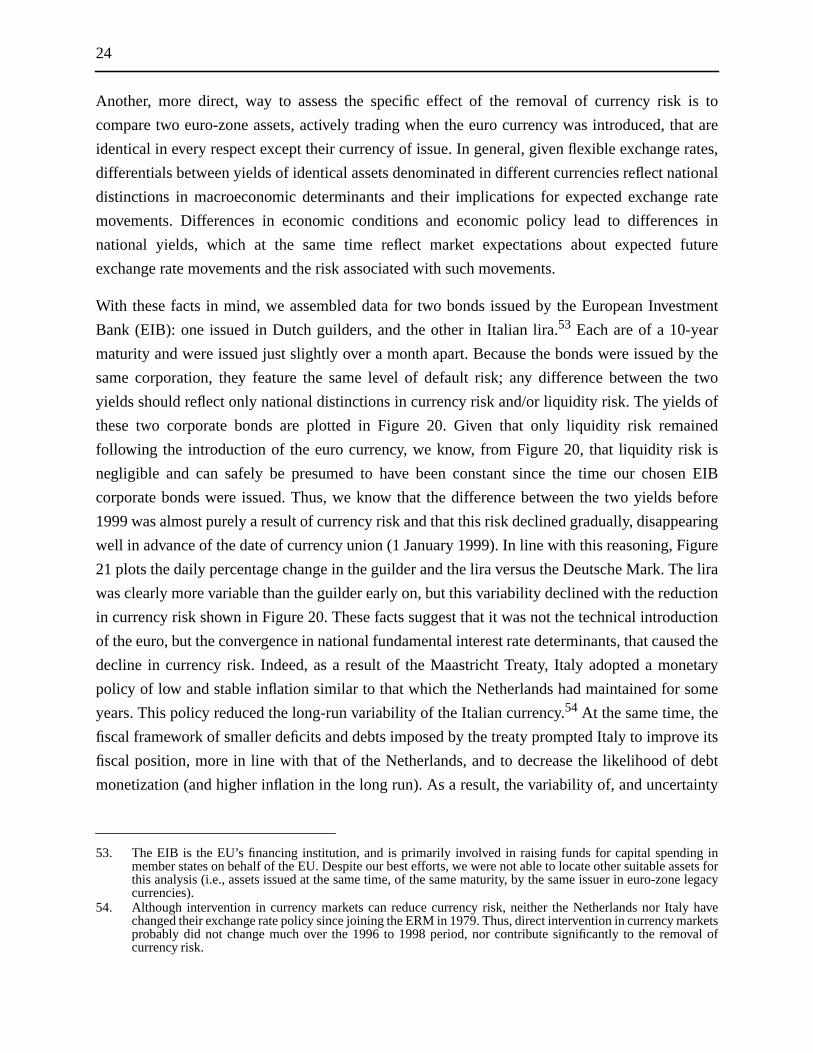
24

is to

hat are

rates,

tional

e rate

es in

future

stment

by the

e two

s of

ined

is

n EIB

before

aring

igure

he lira

ction

ction

sed the

etary

ome

ve its

debt

inty

g insets fore legacy

havearketsval of

Another, more direct, way to assess the specific effect of the removal of currency risk

compare two euro-zone assets, actively trading when the euro currency was introduced, t

identical in every respect except their currency of issue. In general, given flexible exchange

differentials between yields of identical assets denominated in different currencies reflect na

distinctions in macroeconomic determinants and their implications for expected exchang

movements. Differences in economic conditions and economic policy lead to differenc

national yields, which at the same time reflect market expectations about expected

exchange rate movements and the risk associated with such movements.

With these facts in mind, we assembled data for two bonds issued by the European Inve

Bank (EIB): one issued in Dutch guilders, and the other in Italian lira.53 Each are of a 10-year

maturity and were issued just slightly over a month apart. Because the bonds were issued

same corporation, they feature the same level of default risk; any difference between th

yields should reflect only national distinctions in currency risk and/or liquidity risk. The yield

these two corporate bonds are plotted in Figure 20. Given that only liquidity risk rema

following the introduction of the euro currency, we know, from Figure 20, that liquidity risk

negligible and can safely be presumed to have been constant since the time our chose

corporate bonds were issued. Thus, we know that the difference between the two yields

1999 was almost purely a result of currency risk and that this risk declined gradually, disappe

well in advance of the date of currency union (1 January 1999). In line with this reasoning, F

21 plots the daily percentage change in the guilder and the lira versus the Deutsche Mark. T

was clearly more variable than the guilder early on, but this variability declined with the redu

in currency risk shown in Figure 20. These facts suggest that it was not the technical introdu

of the euro, but the convergence in national fundamental interest rate determinants, that cau

decline in currency risk. Indeed, as a result of the Maastricht Treaty, Italy adopted a mon

policy of low and stable inflation similar to that which the Netherlands had maintained for s

years. This policy reduced the long-run variability of the Italian currency.54 At the same time, the

fiscal framework of smaller deficits and debts imposed by the treaty prompted Italy to impro

fiscal position, more in line with that of the Netherlands, and to decrease the likelihood of

monetization (and higher inflation in the long run). As a result, the variability of, and uncerta

53. The EIB is the EU’s financing institution, and is primarily involved in raising funds for capital spendinmember states on behalf of the EU. Despite our best efforts, we were not able to locate other suitable asthis analysis (i.e., assets issued at the same time, of the same maturity, by the same issuer in euro-zoncurrencies).

54. Although intervention in currency markets can reduce currency risk, neither the Netherlands nor Italychanged their exchange rate policy since joining the ERM in 1979. Thus, direct intervention in currency mprobably did not change much over the 1996 to 1998 period, nor contribute significantly to the remocurrency risk.

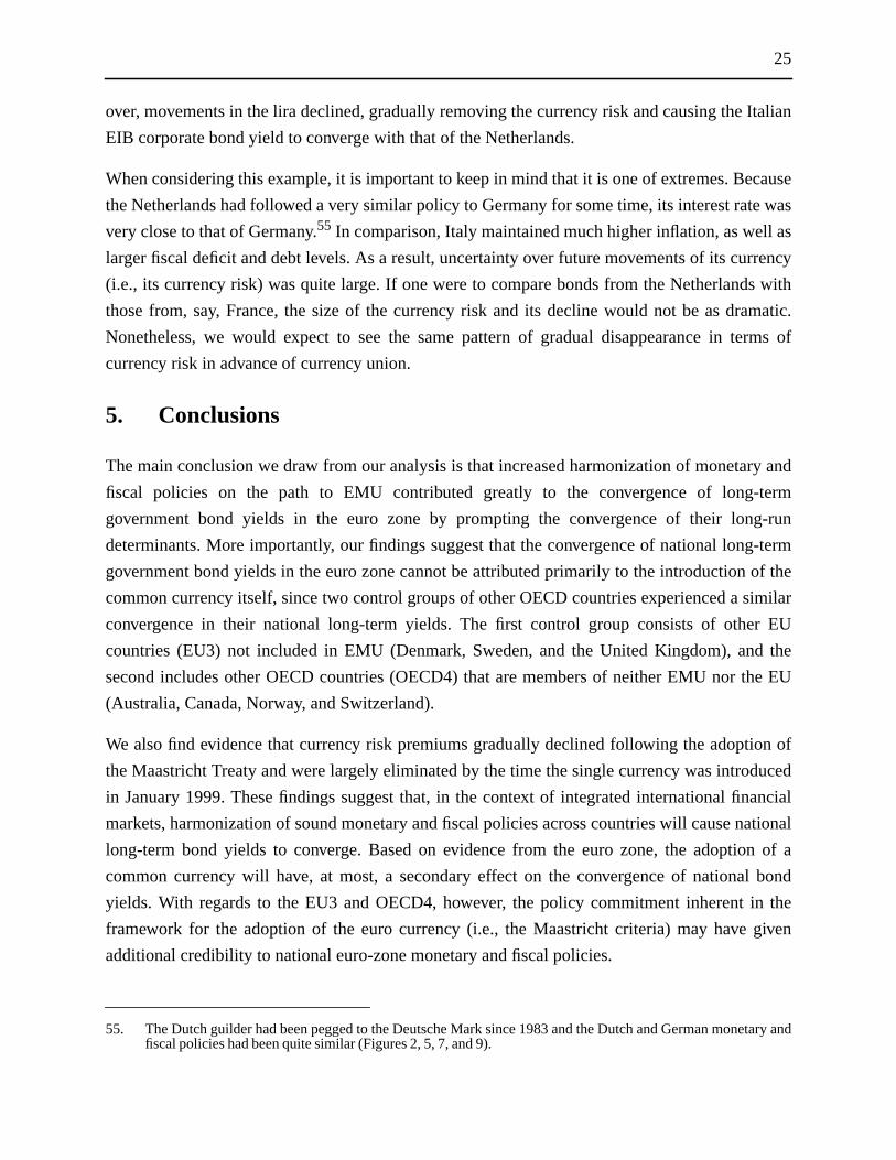
25

talian

ause

was

as

rency

with

matic.

rms of

y and

erm

-run

-term

f the

imilar

EU

the

e EU

n of

uced

ancial

tional

n of a

bond

the

iven

tary and

over, movements in the lira declined, gradually removing the currency risk and causing the I

EIB corporate bond yield to converge with that of the Netherlands.

When considering this example, it is important to keep in mind that it is one of extremes. Bec

the Netherlands had followed a very similar policy to Germany for some time, its interest rate

very close to that of Germany.55 In comparison, Italy maintained much higher inflation, as well

larger fiscal deficit and debt levels. As a result, uncertainty over future movements of its cur

(i.e., its currency risk) was quite large. If one were to compare bonds from the Netherlands

those from, say, France, the size of the currency risk and its decline would not be as dra

Nonetheless, we would expect to see the same pattern of gradual disappearance in te

currency risk in advance of currency union.

5. Conclusions

The main conclusion we draw from our analysis is that increased harmonization of monetar

fiscal policies on the path to EMU contributed greatly to the convergence of long-t

government bond yields in the euro zone by prompting the convergence of their long

determinants. More importantly, our findings suggest that the convergence of national long

government bond yields in the euro zone cannot be attributed primarily to the introduction o

common currency itself, since two control groups of other OECD countries experienced a s

convergence in their national long-term yields. The first control group consists of other

countries (EU3) not included in EMU (Denmark, Sweden, and the United Kingdom), and

second includes other OECD countries (OECD4) that are members of neither EMU nor th

(Australia, Canada, Norway, and Switzerland).

We also find evidence that currency risk premiums gradually declined following the adoptio

the Maastricht Treaty and were largely eliminated by the time the single currency was introd

in January 1999. These findings suggest that, in the context of integrated international fin

markets, harmonization of sound monetary and fiscal policies across countries will cause na

long-term bond yields to converge. Based on evidence from the euro zone, the adoptio

common currency will have, at most, a secondary effect on the convergence of national

yields. With regards to the EU3 and OECD4, however, the policy commitment inherent in

framework for the adoption of the euro currency (i.e., the Maastricht criteria) may have g

additional credibility to national euro-zone monetary and fiscal policies.

55. The Dutch guilder had been pegged to the Deutsche Mark since 1983 and the Dutch and German monefiscal policies had been quite similar (Figures 2, 5, 7, and 9).

26

the

s, we

s. This

d, first

ation

-year

eriod.

ce as a

ominal

as a

ation

ups

ts as

panel

e 10-

ression

f the

e of

-run

ed the

-term

scal

xy the

al U.S.

arket

is also

since

ents

istent

trend

To examine empirically how harmonization of monetary and fiscal policies contributed to

convergence of national long-term government bond yields across euro-zone countrie

assessed how these policies contributed to the convergence of their long-run determinant

entailed examining the determinants across euro-zone countries over the 1980 to 2002 perio

on a country-by-country basis using cointegration techniques, and then using panel estim

techniques to improve the efficiency of the estimated parameters.

On a country-by-country basis, we did not find any evidence of cointegration between the 10

nominal government bond yields and their long-run determinants over the 1980 to 2002 p

The set of long-term determinants that we examined were general government fiscal balan

share of nominal GDP, the stock of accumulated general government debt as a share of n

GDP, expected inflation, and the U.S. or German real 10-year government bond yield

measure of the world real interest rate.

We then examined the trend in 10-year nominal government bond yields using panel estim

over the 1980 to 2002 period for our pool of EMU countries, as well as our two control gro

(EU3 and OECD4) not included in EMU. Considering the same set of long-term determinan

in our country-by-country analysis, we first estimated the long-run parameters using

estimation. We then estimated alternative error-correction models in which the change in th

year nominal government bond yields was regressed on the residuals of the static panel reg

from the first step, along with other stationary variables. In general, we found estimates o

error-correction term that were negative and statistically significant, providing evidenc

cointegration between the 10-year nominal government bond yields and their long

determinants. We also found evidence of real convergence for all countries when we impos

unit restriction on expected inflation, reinforcing the idea that convergence in national long

bond yields is not only the result of monetary policy harmonization but also the result of fi

policy harmonization.

Our euro-zone estimation results also show that, when we use the real German yield to pro

world interest rate, the long-run estimated parameter is three times the size of that of the re

yield, which suggests higher integration of EMU country bond markets with the German m

than that of the United States. The estimated speed of convergence to long-run equilibrium

somewhat faster when using the German yield as opposed to the U.S. yield.

In general, our results suggest that the downward trend in 10-year government bond yields

the early 1980s stems largely from their strong relationship with expected inflation, developm

in the bond yields of the larger countries, and, to a lesser extent, from the effects of pers

changes in general government fiscal balances. Currently, the average yield lies below its

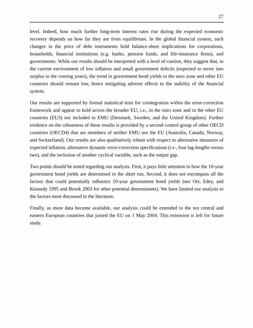
27

omic

such

tions,

, and

at, in

into

er EU

ncial

ction

er EU

ther

OECD

rway,

res of

ersus

-year

all the

, and

sis to

al and

uture

level. Indeed, how much further long-term interest rates rise during the expected econ

recovery depends on how far they are from equilibrium. In the global financial system,

changes in the price of debt instruments hold balance-sheet implications for corpora

households, financial institutions (e.g. banks, pension funds, and life-insurance firms)

governments. While our results should be interpreted with a level of caution, they suggest th

the current environment of low inflation and small government deficits (expected to move

surplus in the coming years), the trend in government bond yields in the euro zone and oth

countries should remain low, hence mitigating adverse effects to the stability of the fina

system.

Our results are supported by formal statistical tests for cointegration within the error-corre

framework and appear to hold across the broader EU; i.e., in the euro zone and in the oth

countries (EU3) not included in EMU (Denmark, Sweden, and the United Kingdom). Fur

evidence on the robustness of these results is provided by a second control group of other

countries (OECD4) that are members of neither EMU nor the EU (Australia, Canada, No

and Switzerland). Our results are also qualitatively robust with respect to alternative measu

expected inflation, alternative dynamic error-correction specifications (i.e., four lag-lengths v

two), and the inclusion of another cyclical variable, such as the output gap.

Two points should be noted regarding our analysis. First, it pays little attention to how the 10

government bond yields are determined in the short run. Second, it does not encompass

factors that could potentially influence 10-year government bond yields (see Orr, Edey

Kennedy 1995 and Brook 2003 for other potential determinants). We have limited our analy

the factors most discussed in the literature.

Finally, as more data become available, our analysis could be extended to the ten centr

eastern European countries that joined the EU on 1 May 2004. This extension is left for f

study.

28

ebt

mic

The

don

cal

hool

.” In

Bibliography

Alesina, A., M. De Broeck, A. Prati, and G. Tabellini. 1993. “Default Risk on Government Din OECD Countries.”Economic Policy: A European Forum October: 428–63.

Alvarez, J. and M. Arellano. 2003. “The Time Series and Cross-Section Asymptotics of DynaPanel Data Estimators.” Econometrica 71(4): 1121–60.

Baltagi, B.H. 2002.Econometric Analysis of Panel Data. New York: John Wiley & Sons Ltd.

Banerjee, A., J.J. Dolado, and R. Mestre. 1993. “On Some Simple Tests for Cointegration: Costs of Simplicity.” Bank of Spain Working Paper No. 9302.

Barro, R.J. 1974. “Are Government Bonds Net Wealth?”Journal of Political Economy 82: 1095–1117.

———. 1989. “The Ricardian Approach to Budget Deficits.”Journal ofEconomic Perspectives3(2): 37–54.

Bernheim, B.D. 1987. “Ricardian Equivalence: An Evaluation of Theory and Evidence.” InNBERMacroeconomics Annual, edited by S. Fischer. Cambridge: MIT Press.

———. 1989. “A Neoclassical Perspective on Budget Deficits.”Journal of Economic Perspec-tives 3(2): 55–72.

Blanchard, O.J. 1985. “Debt, Deficits, and Finite Horizons.”Journal of Political Economy 93(April): 223–46.

Bofinger, P. 2000. “The European Monetary System (1979–1988): Achievements, Flaws anApplicability to Other Regions of the World.” Background paper for special session IVglobal financial issues, UN/ECE Conference,Financing for Development, December2000.

Brook, A.-M. 2003. “Recent and Prospective Trends in Real Long-Term Interest Rates: FisPolicy and Other Drivers.” OECD Economics Department Working Paper No. 367.

Buiter, W.H. 1988. “Death, Birth, Productivity Growth and Debt Neutrality.”The Economic Jour-nal 98 (391): 279–93.

Caramazza, F., K. Clinton, A. Côté, and D. Longworth. 1986.International Capital Mobility andAsset Substitutability: Some Theory and Evidence on Recent Structural Changes. Techni-cal Report No. 44. Ottawa: Bank of Canada.

Carlson, J.A. and C.L. Osler. 1999. “Determinants of Currency Risk Premiums.” Krannert Scof Management and Federal Reserve Bank of New York.

Carlson, J.A. and M. Parkin. 2001. “Inflation Expectations.”Economica (May): 123–38.

Cebula, R. 2000. “Impact of Budget Deficits on Ex-Post Real Long-Term Interest Rates.”AppliedEconomic Letters7(3): 177–79.

Codogno, L., C. Favero, and A. Missale. 2003. “Yield Spreads on EMU Government BondsEMU: Assessing the Impact of the Euro, edited by R. Baldwin, 211–40.

29

Link?

ork,

ro-

es.”

n,

rme.”

ionso.

Tax

ing

rt-

truc-

ty

ity.”

Correia-Nunes, J. and L. Stemitsiotis. 1995. “Budget Deficit and Interest Rates: Is There a International Evidence.”Oxford Bulletin of Economics and Statistics 57(4): 425–49.

Davidson, R. and J.G. MacKinnon. 1993. “Estimation and Inference in Econometrics.” New YOxford: Oxford University Press.

de Bandt, O. and F.P. Mongelli. 2000. “Convergence of Fiscal Policies in the Euro Area.” Eupean Central Bank Working Paper No. 20.

Diamond, P.A. 1965. “National Debt and Neoclassical Economic Growth.”American EconomicReview 55: 1125–50.

Durré, A., S. Evjen, and R. Pilegaard. 2003. “Estimating Risk Premia in Money Market RatEuropean Central Bank Working Paper No. 221.

Engle, R.F. and C.W.J. Granger. 1987. “Co-Integration and Error Correction: RepresentatioEstimation and Testing.” Econometrica 55: 251–76.

European Central Bank. 2003. ECB Monthly Bulletin, November.

Fillion, J.-F. 1996. “L’endettement du Canada et ses effets sur les taux d’intérêts de long teDocument de travail de la Banque du Canada, No. 96-14.

Fukao, M. and M. Hanazaki. 1986. “Internationalisation of Financial Markets: Some Implicatfor Macroeconomic Policy and for the Allocation of Capital.” OECD Working Paper N37.

Gale, W.G. and P.R. Orszag. 2002. “The Economic Effects of Long-Term Fiscal Discipline.”Policy Center, Urban Institute and Brookings Institution.

Gali, J. and R. Perotti. 2003. “Fiscal Policy and Monetary Integration in Europe.” NBER WorkPaper No. 9773.

Gjersem, C. 2003. “Financial Market Integration in the Euro Area.” OECD Economics Depament Working Paper No. 368.

Goldberg, L.G., J.R. Lothian, and J. Okunev. 2003. “Has International Financial IntegrationIncreased?”Open Economies Review 14: 299–317.

Granger, C.W.J. and P. Newbold. 1974. “Spurious Regressions in Econometrics.”Journal ofEconometrics2: 111–20.

Hartmann, P., A. Maddaloni, and S. Manganelli. 2003. “The Euro Area Financial System: Sture, Integration and Policy Initiatives.” ECB Working Paper No. 230.

Haug, A.A. 1992. “Critical Values for theZα - Phillips-Ouliaris Test for Cointegration.”OxfordBulletin of Economics and Statistics 54(3): 473–80.

Hsiao, C. 1990.Analysis of Panel Data. Econometric Society Monographs, Cambridge UniversiPress.

Knot, K. and J. de Haan. 1995. “Fiscal Policy and Interest Rates in the European CommunEuropean Journal of Political Economy 11(1): 171–87.

30

s.”

ent

acro

gmic

eries

for

m

ence.”

r

rest

Laubach, T. 2003. “New Evidence on the Interest Rate Effects of Budget Deficits and DebtBoard of Governors of the Federal Reserve System Working Paper No. 2003-12.

MacKinnon, J.G. 1991. “Critical Values for Cointegration Tests.” InLong-Run Economic Rela-tionships: Readings in Cointegration, edited by R. Engle and C. Granger, Chapter 13.Oxford: Oxford University Press.

Macklem, T. 1994–1995. “Some Macroeconomic Implications of Rising Levels of GovernmDebt.” Bank of Canada Review (Winter): 41–60.

Macklem, T., D. Rose, and R. Tetlow. 1995. “Government Debt and Deficits in Canada: A MSimulation Analysis.” Bank of Canada Working Paper No. 95-4.

Masson, P., T. Bayoumi, and H. Samiei. 1995. “Saving Behavior in Industrial and DevelopinCountries.” World Economic and Financial Surveys, Staff Studies for the World EconoOutlook (September). Chapter I, 1-27. IMF.

Moody’s Investors Service. 2003. “Sovereign Bond Defaults, Rating Transitions and Recov(1985-2002).”Special Comment, February.

Nickell, S. 1981. “Biases in Dynamic Models with Fixed Effects.”Econometrica 49: 1417–26.

Ng, S. and P. Perron. 1995. “Unit Root Tests in ARMA Models with Data Dependent Methodsthe Selection of the Truncation Lag.”Journal of the American Statistical Association90(429): 268–81.

OECD. 2003.OECD Economic Outlook 2(74): December.

Orr, A., M. Edey, and M. Kennedy. 1995. “Real Long-Term Interest Rates: The Evidence froPooled-Time-Series.” OECD Economic Studies No. 25, 1995/II: 75–107.

Phillips, P.C.B. 1986. “Understanding Spurious Regressions in Econometrics.”Journal ofEconometrics33(3): 311–40.

Phillips, P.C.B. and P. Perron. 1988. “Testing for a Unit Root in Time Series Regression.”Biomet-rica 75: 335–46.

Pigott, C. 1994. “International Interest Rate Convergence: A Survey of the Issues and EvidFederal Reserve Bank of New York.

Stock, J.H. and M.W. Watson. 1993. “A Simple Estimator of Cointegrating Vectors in HigheOrder Integrated Systems.”Econometrica 61(4): 783–820.

Throop, A.W. 1994. “International Financial Market Integration and Linkages of National InteRates.” Federal Reserve Bank of San Francisco,Economic Review 3: 3–18.

Weil, P. 1989. “Overlapping Families of Infinitely-Lived Agents.”Journal of Public Economics38 (March): 183–98.

Yaari, M.E. 1965. “Uncertain Lifetime, Life Insurance, and the Theory of the Consumer.”Reviewof Economic Studies 32 (April) 137–50.

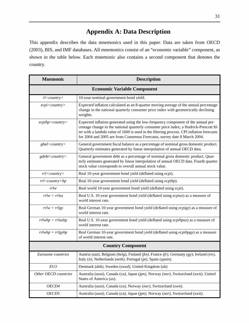
31

OECD

nt, as

tes the

tageg

r-tt fil-sts

duct.

uar-rter

Appendix A: Data Description

This appendix describes the data mnemonics used in this paper. Data are taken from

(2003), BIS, and IMF databases. All mnemonics consist of an “economic variable” compone

shown in the table below. Each mnemonic also contains a second component that deno

country.

Mnemonic Description

Economic Variable Component

rl<country> 10-year nominal government bond yield.

ecpi<country> Expected inflation calculated as an 8-quarter moving average of the annual percenchange in the national quarterly consumer price index with geometrically declininweights.

ecpihp<country> Expected inflation generated using the low-frequency component of the annual pecentage change in the national quarterly consumer price index; a Hodrick-Prescoter with a lambda value of 1600 is used in the filtering process. CPI inflation forecafor 2004 and 2005 are from Consensus Forecasts, survey date 8 March 2004.

gbal<country> General government fiscal balance as a percentage of nominal gross domestic proQuarterly estimates generated by linear interpolation of annual OECD data.

gdebt<country> General government debt as a percentage of nominal gross domestic product. Qterly estimates generated by linear interpolation of annual OECD data. Fourth quastock value corresponds to overall annual stock value.

rrl<country> Real 10-year government bond yield (deflated usingecpi).

rrl<country>hp Real 10-year government bond yield (deflated usingecpihp).

rrlw Real world 10-year government bond yield (deflated usingecpi).

rrlw = rrlus Real U.S. 10-year government bond yield (deflated usingecpius) as a measure ofworld interest rate.

rrlw = rrlgy Real German 10-year government bond yield (deflated usingecpigy) as a measure ofworld interest rate.

rrlwhp = rrlushp Real U.S. 10-year government bond yield (deflated usingecpihpus) as a measure ofworld interest rate.

rrlwhp = rrlgyhp Real German 10-year government bond yield (deflated usingecpihpgy) as a measureof world interest rate.

Country Component

Eurozone countries Austria (aut), Belgium (belg), Finland (fin), France (fr), Germany (gy), Ireland (ire),Italy (it), Netherlands (neth),Portugal (pt), Spain (spain).

EU3 Denmark (dnk),Sweden (swed),United Kingdom (uk).

Other OECD countries Australia (aust),Canada (ca),Japan (jpn), Norway (nor), Switzerland (swit),UnitedStates of America (us).

OECD4 Australia (aust),Canada (ca),Norway (nor), Switzerland (swit).

OECD5 Australia (aust),Canada (ca),Japan (jpn), Norway (nor), Switzerland (swit).

32

I. In

Italy,

by

7, the

mong

tal. In

rland,

rt to

ropean

ears

onomic

etary

o limit

When

“the

the

ained

ificant

ing the

etary

ghout

U), a

uced,

t at a

nited

n a

2 per

7, the

ong

Appendix B: Timeline for Economic and Monetary Union

As illustrated in Chart B1, the long path to EMU was born out of the ashes of World War I

1952, only three years after the end of post-war reconstruction, “the Six” (Germany, France,

Belgium, Luxembourg, and the Netherlands) took a critical step in reunifying Europe

establishing the European Coal and Steel Community (ECSC). Five years later, in 195

Treaty of Rome was signed, creating the European Economic Community (EEC) which, a

other things, marked the beginning of the push towards free movement of labour and capi

1960, several European countries (Austria, Denmark, Norway, Portugal, Sweden, Switze

and the United Kingdom) formed the European Free Trade Association (EFTA) in an effo

liberalize trade and counterbalance the EEC. The ECSC and the EEC (as well as the Eu

Atomic Energy Community) merged in 1967, to form the European Community (EC). Two y

later, the first agreement was made among EC member states to coordinate short-term ec

policies.

In 1970, the Werner Report laid out, for the first time, the eventual steps to European mon

union. In 1972, “the snake” exchange rate system was introduced, wherein the Six agreed t

the margin of currency fluctuations to a 4.5 per cent band around an agreed central parity.

the United Kingdom, Ireland, and Denmark acceded to the EC in 1973, they also joined

snake.” However, this first attempt at European exchange rate coordination fell victim to

effects of the oil-price crises in the late 1970s. By 1978, only five of nine member states rem

on “the snake.” The mid-1970s had, nonetheless, brought progress on another front. A sign

free trade agreement had been reached in 1974 between the EC and the EFTA, broaden

scope of trade liberalization across western Europe.

The experience of “the snake” paved the way for the establishment of the European Mon

System (EMS) in 1979, leading to the beginning of the empirical sample period used throu

this paper (1980 to 2002). Within the EMS, the concept of the European Currency Unit (EC

virtual currency based on relative GNP and trade values for all EC countries, was introd

along with the exchange rate mechanism (ERM). The ERM marked the second attemp

coordinated EC exchange rate policy and initially included all EC countries except the U

Kingdom. Participants in the ERM were originally permitted, like “the snake,” to move withi

4.5 per cent band around a central parity with the ECU, except for Italy, which adopted a 1

cent band because of its higher inflation rate.

In 1981, Greece acceded to the EC, followed five years later by Spain and Portugal. In 198

original Treaty of Rome was modified by the Single European Act, which formalized, am

33

labour,

, and

nd of

espite

992,

the

ibility

1996,

3.

rs of

MU):

ber

rgence

t the

l euro

reaty

re than

terms

points

s

, Italy,

other things, the plan to create a single European economic market in goods and services,

and capital by the end of 1992. The ERM expanded to include Spain, the United Kingdom

Portugal in 1989, 1990, and 1992, respectively, although using the wider 12 per cent ba

fluctuation (Italy had, meanwhile, adopted the standard 4.5 per cent band in 1990). D

several revaluations within the ERM, the mechanism functioned relatively smoothly until 1

when speculative currency attacks forced the United Kingdom and Italy to withdraw from

arrangement. The following year, a new 30 per cent band was adopted to provide added flex

and reduce the threat of speculative attacks. Italy subsequently rejoined the ERM in

whereas the United Kingdom has since abstained.

The European Union (EU) as we know it today was born out of the Maastricht Treaty in 19956

Besides enacting a common foreign and security policy, and dealing with EU-level matte

justice, this treaty specified the three steps required for Economic and Monetary Union (E

by the end of 1993, capital flows were to be completely freed within the EU; by 1999, mem

states preparing to adopt the euro currency upon its launch had to satisfy a set of conve

criteria by which major economic policies were coordinated across nations; effective a

beginning of 1999, the European Central Bank would be established, along with the officia

currency for which member-country conversion rates were irrevocably set. The Maastricht T

convergence criteria were as follows:

• the ratio of general government deficit to GDP must not exceed 3 per cent

• the ratio of gross general government debt to GDP must not exceed 60 per cent

• the average inflation rate over the year before assessment must not exceed by mo

1.5 percentage points the average of the three best performing member states in

of price stability

• the long-term nominal interest rate must not exceed by more than 2 percentage

the average of the three best performing member states in terms of price stability

• the ERM must be respected without severe tensions for at least the last two year

before assessment (30 per cent band around the ECU)

56. The original member states of the EU were Belgium, Denmark, France, Germany, Greece, IrelandLuxembourg, the Netherlands, Portugal, Spain, and the United Kingdom.

34

nging

f

om,

euro

going

Pact

ntly,

ty in

the

y hastionaliled toursued

stonia,pt the

as aventuallow a

stonia,new

r cent

In 1995, three new members were admitted to the EU (Austria, Finland, and Sweden), bri

the total number of member states to 15.57,58At the launch of the euro in 1999, EMU consisted o

11 of the 15 EU countries; those that did not participate in EMU were the United Kingd

Sweden, Denmark, and Greece (Greece later joined in 2001).59 By the beginning of 2002, all

former national currencies (also known as “legacy” currencies) were phased out and the

became the sole legal currency in EMU member states.

Now that monetary integration has been realized in much of western Europe, the on

challenge is for all EU member countries to continuously meet the Stability and Growth

(primarily, the first two conditions of the Maastricht Treaty convergence criteria). Curre

several members of EMU (including Germany, France, and Italy) are experiencing difficul

maintaining a deficit-to-GDP ratio below the 3 per cent limit and a debt-to-GDP ratio below

60 per cent maximum.60

57. Norway and Switzerland, while remaining members of the EFTA, are not members of the EU. Norwaapplied twice for accession. The first application was submitted in 1967 but was rejected in a nareferendum in 1972. In 1992, Norway again applied for membership, but a second referendum in 1994 fapass. Switzerland applied for membership in 1992 and maintains an open invitation, but has not actively pmembership.

58. Ten new European countries joined the EU on 1 May 2004: Poland, Hungary, the Czech Republic, ELatvia, Lithuania, Slovakia, Slovenia, Cyprus, and Malta. New members are required to eventually adoeuro and will, thus, have to satisfy the convergence criteria, including the current version of the ERM.

59. In sync with the second stage of EMU, 1999 marked the introduction of ERMII, which replaced the ERMvoluntary means for non-EMU members of the EU to reduce exchange rate fluctuations and prepare for eadoption of the euro. Currently, Denmark is the only nation participating in ERMII, and has elected to fol4.5 per cent band around the euro, as opposed to the minimum requirement of a 30 per cent band. ELithuania, Slovenia, and Cyprus are expected to apply in 2004 for entrance into ERMII with the remainingcentral and eastern European EU members to follow.

60. Italy is a special case, in that it was admitted to EMU with a debt-to-GDP limit far exceeding the 60 pelimit, on the condition that this level be reduced over time.

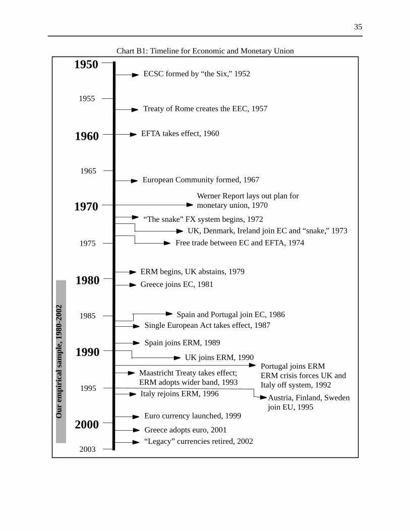
35

Chart B1: Timeline for Economic and Monetary Union

1950

1955

2003

1960

1970

1980

1990

2000

1965

1975

1985

1995

Treaty of Rome creates the EEC, 1957

EFTA takes effect, 1960

European Community formed, 1967

Werner Report lays out plan formonetary union, 1970

ECSC formed by “the Six,” 1952

“The snake” FX system begins, 1972

ERM begins, UK abstains, 1979

Single European Act takes effect, 1987

Maastricht Treaty takes effect;ERM adopts wider band, 1993

Euro currency launched, 1999

UK, Denmark, Ireland join EC and “snake,” 1973

Free trade between EC and EFTA, 1974

Greece joins EC, 1981

Spain and Portugal join EC, 1986

Spain joins ERM, 1989

UK joins ERM, 1990Portugal joins ERMERM crisis forces UK andItaly off system, 1992

Italy rejoins ERM, 1996 Austria, Finland, Swedenjoin EU, 1995

Greece adopts euro, 2001

“Legacy” currencies retired, 2002

Our

em

piric

al s

ampl

e, 1

980-

2002

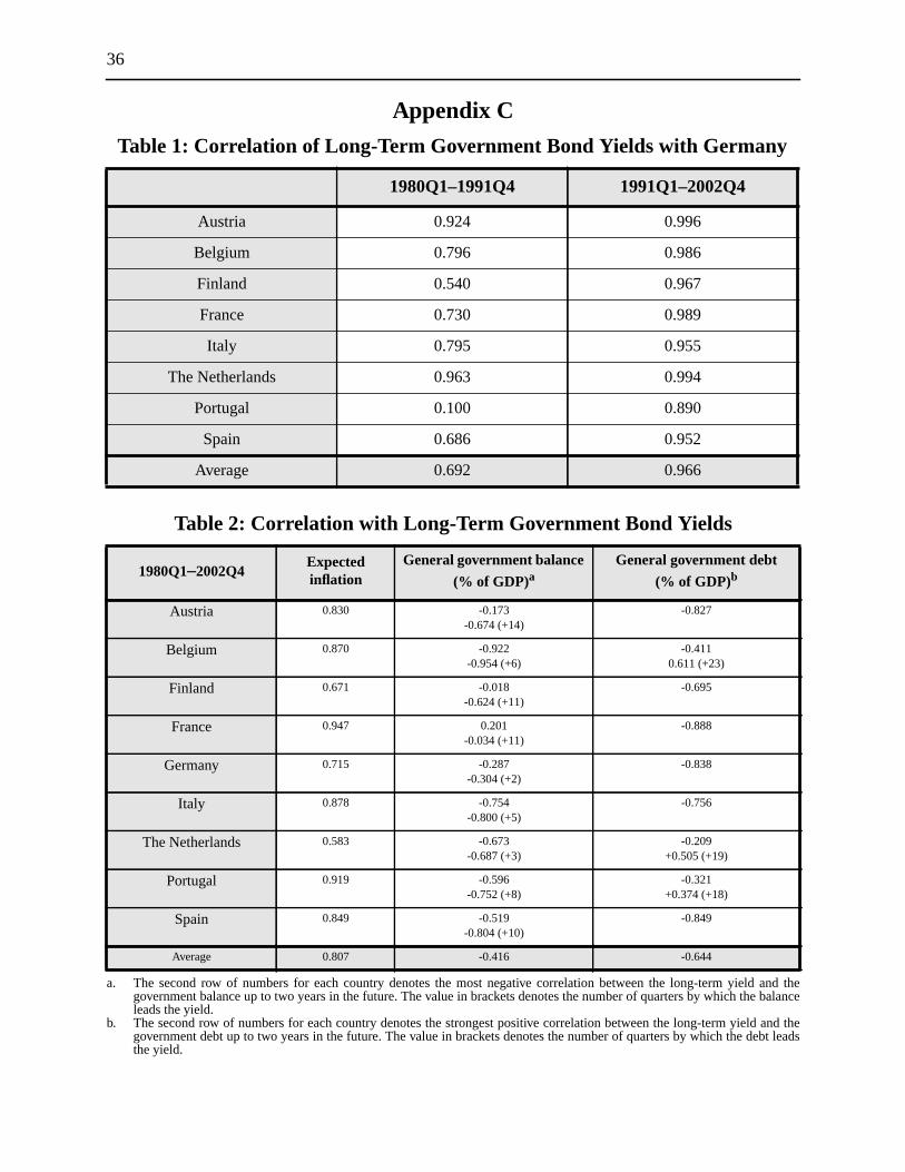
36

and thebalance

and thebt leads

Appendix C

Table 1: Correlation of Long-Term Government Bond Yields with Germany

1980Q1–1991Q4 1991Q1–2002Q4

Austria 0.924 0.996

Belgium 0.796 0.986

Finland 0.540 0.967

France 0.730 0.989

Italy 0.795 0.955

The Netherlands 0.963 0.994

Portugal 0.100 0.890

Spain 0.686 0.952

Average 0.692 0.966

Table 2: Correlation with Long-Term Government Bond Yields

1980Q1–2002Q4Expectedinflation

General government balance

(% of GDP)a

a. The second row of numbers for each country denotes the most negative correlation between the long-term yieldgovernment balance up to two years in the future. The value in brackets denotes the number of quarters by which theleads the yield.

General government debt

(% of GDP)b

b. The second row of numbers for each country denotes the strongest positive correlation between the long-term yieldgovernment debt up to two years in the future. The value in brackets denotes the number of quarters by which the dethe yield.

Austria 0.830 -0.173-0.674 (+14)

-0.827

Belgium 0.870 -0.922-0.954 (+6)

-0.4110.611 (+23)

Finland 0.671 -0.018-0.624 (+11)

-0.695

France 0.947 0.201-0.034 (+11)

-0.888

Germany 0.715 -0.287-0.304 (+2)

-0.838

Italy 0.878 -0.754-0.800 (+5)

-0.756

The Netherlands 0.583 -0.673-0.687 (+3)

-0.209+0.505 (+19)

Portugal 0.919 -0.596-0.752 (+8)

-0.321+0.374 (+18)

Spain 0.849 -0.519-0.804 (+10)

-0.849

Average 0.807 -0.416 -0.644

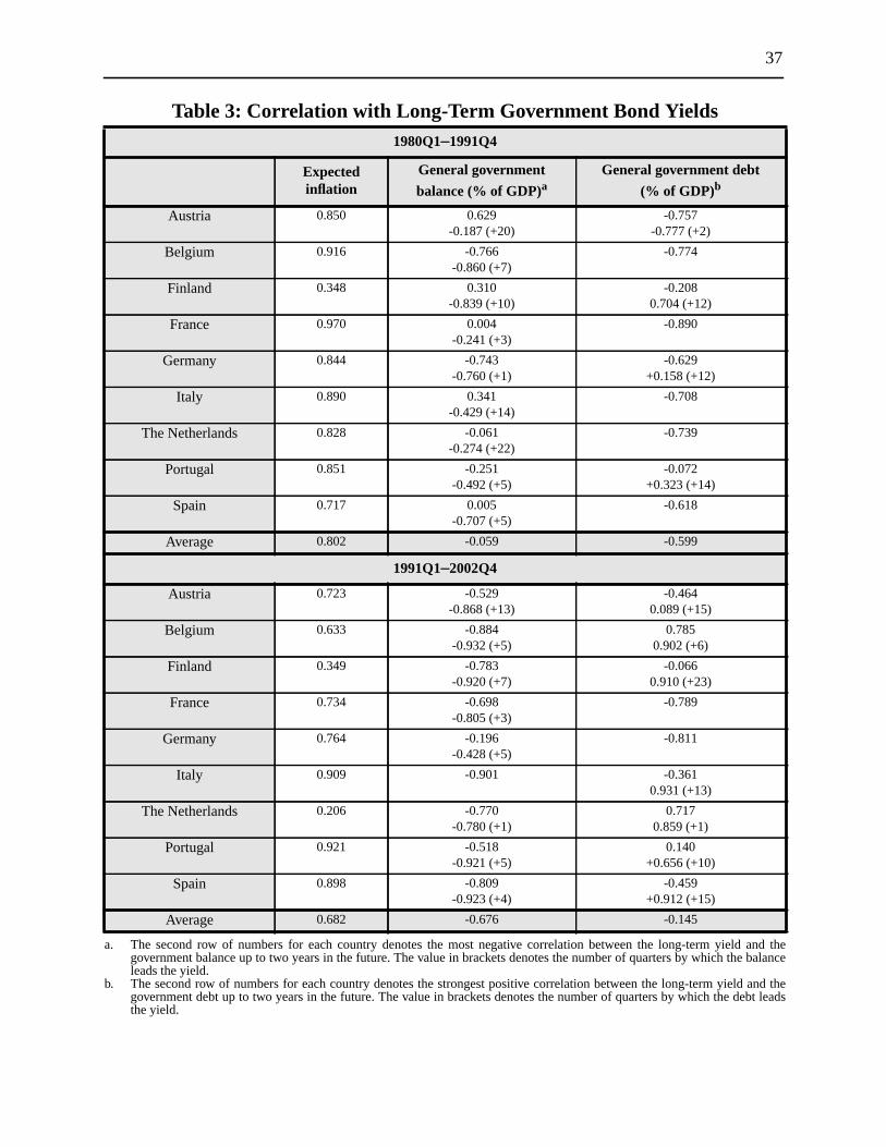
37

and thebalance

and theebt leads

Table 3: Correlation with Long-Term Government Bond Yields1980Q1–1991Q4

Expectedinflation

General government

balance (% of GDP)a

a. The second row of numbers for each country denotes the most negative correlation between the long-term yieldgovernment balance up to two years in the future. The value in brackets denotes the number of quarters by which theleads the yield.

General government debt

(% of GDP)b

b. The second row of numbers for each country denotes the strongest positive correlation between the long-term yieldgovernment debt up to two years in the future. The value in brackets denotes the number of quarters by which the dthe yield.

Austria 0.850 0.629-0.187 (+20)

-0.757-0.777 (+2)

Belgium 0.916 -0.766-0.860 (+7)

-0.774

Finland 0.348 0.310-0.839 (+10)

-0.2080.704 (+12)

France 0.970 0.004-0.241 (+3)

-0.890

Germany 0.844 -0.743-0.760 (+1)

-0.629+0.158 (+12)

Italy 0.890 0.341-0.429 (+14)

-0.708

The Netherlands 0.828 -0.061-0.274 (+22)

-0.739

Portugal 0.851 -0.251-0.492 (+5)

-0.072+0.323 (+14)

Spain 0.717 0.005-0.707 (+5)

-0.618

Average 0.802 -0.059 -0.599

1991Q1–2002Q4

Austria 0.723 -0.529-0.868 (+13)

-0.4640.089 (+15)

Belgium 0.633 -0.884-0.932 (+5)

0.7850.902 (+6)

Finland 0.349 -0.783-0.920 (+7)

-0.0660.910 (+23)

France 0.734 -0.698-0.805 (+3)

-0.789

Germany 0.764 -0.196-0.428 (+5)

-0.811

Italy 0.909 -0.901 -0.3610.931 (+13)

The Netherlands 0.206 -0.770-0.780 (+1)

0.7170.859 (+1)

Portugal 0.921 -0.518-0.921 (+5)

0.140+0.656 (+10)

Spain 0.898 -0.809-0.923 (+4)

-0.459+0.912 (+15)

Average 0.682 -0.676 -0.145

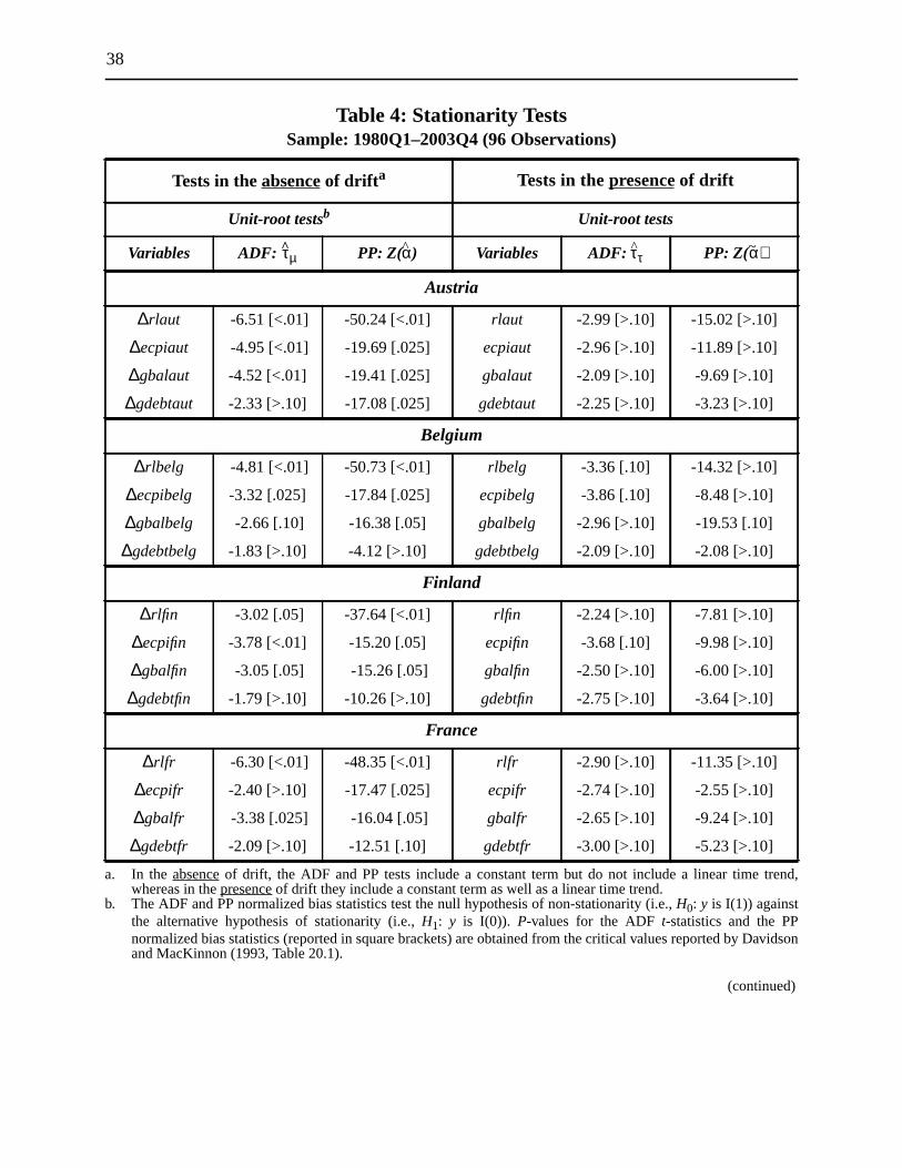
38

trend,

avidson

Table 4: Stationarity TestsSample: 1980Q1–2003Q4 (96 Observations)

Tests in theabsence of drifta

a. In theabsence of drift, the ADF and PP tests include a constant term but do not include a linear timewhereas in thepresence of drift they include a constant term as well as a linear time trend.

Tests in thepresence of drift

Unit-root testsb

b. The ADF and PP normalized bias statistics test the null hypothesis of non-stationarity (i.e.,H0: y is I(1)) againstthe alternative hypothesis of stationarity (i.e.,H1: y is I(0)). P-values for the ADFt-statistics and the PPnormalized bias statistics (reported in square brackets) are obtained from the critical values reported by Dand MacKinnon (1993, Table 20.1).

Unit-root tests

Variables ADF: τµ PP: Z(α) Variables ADF: ττ PP: Z(~α)

Austria

∆rlaut -6.51 [<.01] -50.24 [<.01] rlaut -2.99 [>.10] -15.02 [>.10]

∆ecpiaut -4.95 [<.01] -19.69 [.025] ecpiaut -2.96 [>.10] -11.89 [>.10]

∆gbalaut -4.52 [<.01] -19.41 [.025] gbalaut -2.09 [>.10] -9.69 [>.10]

∆gdebtaut -2.33 [>.10] -17.08 [.025] gdebtaut -2.25 [>.10] -3.23 [>.10]

Belgium

∆rlbelg -4.81 [<.01] -50.73 [<.01] rlbelg -3.36 [.10] -14.32 [>.10]

∆ecpibelg -3.32 [.025] -17.84 [.025] ecpibelg -3.86 [.10] -8.48 [>.10]

∆gbalbelg -2.66 [.10] -16.38 [.05] gbalbelg -2.96 [>.10] -19.53 [.10]

∆gdebtbelg -1.83 [>.10] -4.12 [>.10] gdebtbelg -2.09 [>.10] -2.08 [>.10]

Finland

∆rlfin -3.02 [.05] -37.64 [<.01] rlfin -2.24 [>.10] -7.81 [>.10]

∆ecpifin -3.78 [<.01] -15.20 [.05] ecpifin -3.68 [.10] -9.98 [>.10]

∆gbalfin -3.05 [.05] -15.26 [.05] gbalfin -2.50 [>.10] -6.00 [>.10]

∆gdebtfin -1.79 [>.10] -10.26 [>.10] gdebtfin -2.75 [>.10] -3.64 [>.10]

France

∆rlfr -6.30 [<.01] -48.35 [<.01] rlfr -2.90 [>.10] -11.35 [>.10]

∆ecpifr -2.40 [>.10] -17.47 [.025] ecpifr -2.74 [>.10] -2.55 [>.10]

∆gbalfr -3.38 [.025] -16.04 [.05] gbalfr -2.65 [>.10] -9.24 [>.10]

∆gdebtfr -2.09 [>.10] -12.51 [.10] gdebtfr -3.00 [>.10] -5.23 [>.10]

(continued)

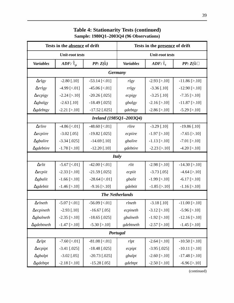
39

Table 4: Stationarity Tests (continued)Sample: 1980Q1–2003Q4 (96 Observations)

Tests in theabsence of drift Tests in thepresence of drift

Unit-root tests Unit-root tests


Germany

∆rlgy -2.80 [.10] -53.14 [<.01] rlgy -2.93 [>.10] -11.86 [>.10]

∆rrlgy -4.99 [<.01] -45.06 [<.01] rrlgy -3.36 [.10] -12.90 [>.10]

∆ecpigy -2.24 [>.10] -20.26 [.025] ecpigy -3.25 [.10] -7.35 [>.10]

∆gbalgy -2.63 [.10] -18.49 [.025] gbalgy -2.16 [>.10] -11.87 [>.10]

∆gdebtgy -2.21 [>.10] -17.52 [.025] gdebtgy -2.86 [>.10] -5.29 [>.10]

Ireland (1985Q1–2003Q4)

∆rlire -4.86 [<.01] -48.60 [<.01] rlire -3.29 [.10] -19.86 [.10]

∆ecpiire -3.02 [.05] -19.82 [.025] ecpiire -1.97 [>.10] -7.65 [>.10]

∆gbalire -3.34 [.025] -14.69 [.10] gbalire -1.13 [>.10] -7.01 [>.10]

∆gdebtire -1.78 [>.10] -12.20 [.10] gdebtire -2.23 [>.10] -4.20 [>.10]

Italy

∆rlit -5.67 [<.01] -42.00 [<.01] rlit -2.98 [>.10] -14.30 [>.10]

∆ecpiit -2.33 [>.10] -21.59 [.025] ecpiit -3.73 [.05] -4.64 [>.10]

∆gbalit -1.66 [>.10] -28.64 [<.01] gbalit -1.99 [>.10] -6.17 [>.10]

∆gdebtit -1.46 [>.10] -9.16 [>.10] gdebtit -1.85 [>.10] -1.16 [>.10]

The Netherlands

∆rlneth -5.07 [<.01] -56.09 [<.01] rlneth -3.18 [.10] -11.00 [>.10]

∆ecpineth -2.93 [.10] -16.67 [.05] ecpineth -3.12 [>.10] -5.96 [>.10]

∆gbalneth -2.35 [>.10] -18.65 [.025] gbalneth -1.92 [>.10] -12.16 [>.10]

∆gdebtneth -1.47 [>.10] -5.30 [>.10] gdebtneth -2.57 [>.10] -1.45 [>.10]

Portugal

∆rlpt -7.60 [<.01] -81.08 [<.01] rlpt -2.64 [>.10] -10.50 [>.10]

∆ecpipt -3.41 [.025] -18.48 [.025] ecpipt -3.95 [.025] -10.11 [>.10]

∆gbalpt -3.02 [.05] -20.73 [.025] gbalpt -2.60 [>.10] -17.48 [>.10]

∆gdebtpt -2.18 [>.10] -15.28 [.05] gdebtpt -2.50 [>.10] -6.96 [>.10]

(continued)

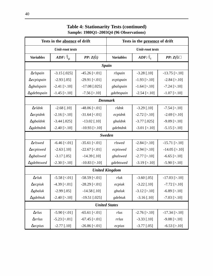
40

Tests in theabsence of drift Tests in thepresence of drift

Unit-root tests Unit-root tests


Spain

∆rlspain -3.15 [.025] -45.26 [<.01] rlspain -3.28 [.10] -13.75 [>.10]

∆ecpispain -2.93 [.05] -29.91 [<.01] ecpispain -1.93 [>.10] -2.84 [>.10]

∆gbalspain -2.41 [>.10] -17.08 [.025] gbalspain -1.64 [>.10] -7.24 [>.10]

∆gdebtspain -1.45 [>.10] -7.56 [>.10] gdebtspain -2.54 [>.10] -1.07 [>.10]

Denmark

∆rldnk -2.68 [.10] -48.06 [<.01] rldnk -3.29 [.10] -7.54 [>.10]

∆ecpidnk -2.16 [>.10] -31.64 [<.01] ecpidnk -2.72 [>.10] -2.69 [>.10]

∆gbaldnk -3.44 [.025] -13.02 [.10] gbaldnk -3.77 [.025] -9.09 [>.10]

∆gdebtdnk -2.40 [>.10] -10.93 [>.10] gdebtdnk -3.01 [>.10] -5.15 [>.10]

Sweden

∆rlswed -6.46 [<.01] -35.61 [<.01] rlswed -2.84 [>.10] -15.71 [>.10]

∆ecpiswed -2.63 [.10] -22.67 [<.01] ecpiswed -2.94 [>.10] -14.05 [>.10]

∆gbalswed -3.17 [.05] -14.39 [.10] gbalswed -2.77 [>.10] -6.65 [>.10]

∆gdebtswed -2.30 [>.10] -10.83 [>.10] gdebtswed -3.19 [>.10] -5.90 [>.10]

United Kingdom

∆rluk -5.58 [<.01] -58.59 [<.01] rluk -3.60 [.05] -17.03 [>.10]

∆ecpiuk -4.39 [<.01] -28.29 [<.01] ecpiuk -3.22 [.10] -7.72 [>.10]

∆gbaluk -2.99 [.05] -14.58 [.10] gbaluk -3.12 [>.10] -6.89 [>.10]

∆gdebtuk -2.40 [>.10] -19.51 [.025] gdebtuk -3.16 [.10] -7.03 [>.10]

United States

∆rlus -5.90 [<.01] -65.61 [<.01] rlus -2.76 [>.10] -17.34 [>.10]

∆rrlus -5.23 [<.01] -67.45 [<.01] rrlus -3.33 [.10] -9.08 [>.10]

∆ecpius -2.77 [.10] -26.86 [<.01] ecpius -3.77 [.05] -6.53 [>.10]

Table 4: Stationarity Tests (continued)Sample: 1980Q1–2003Q4 (96 Observations)

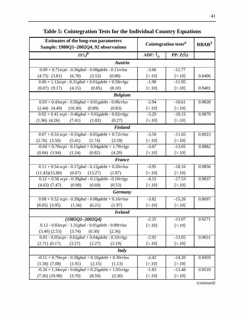
41

Table 5: Cointegration Tests for the Individual Country Equations

Estimates of the long-run parametersSample: 1980Q1–2002Q4, 92 observations

Cointegration testsa RBAR2

(αSt)b ADF: τµ PP: Z(α)

Austria

0.09 + 0.71ecpi - 0.56gbal - 0.08gdebt - 0.11rrlus

(4.75) (3.81) (6.78) (3.53) (0.88)

-3.66

[>.10]

-11.77

[>.10] 0.84060.00 + 1.12ecpi - 0.31gbal + 0.01gdebt + 0.58rrlgy

(0.07) (9.17) (4.15) (0.85) (8.10)

-1.98

[>.10]

-11.95

[>.10] 0.9401

Belgium

0.03 + 0.43ecpi - 0.50gbal + 0.01gdebt - 0.06rrlus

(2.44) (4.49) (10.30) (0.89) (0.83)

-2.94

[>.10]

-18.61

[>.10]

0.9828

0.02 + 0.41ecpi - 0.46gbal + 0.02gdebt - 0.02rrlgy

(1.96) (4.26) (7.41) (1.82) (0.27)

-3.29

[>.10]

-18.15

[>.10]

0.9879

Finland

0.07 + 0.53 ecpi - 0.55gbal - 0.05gdebt + 0.72rrlus

(2.76) (3.50) (5.41) (1.74) (3.59)

-3.59

[>.10]

-11.65

[>.10]

0.8923

-0.04 + 0.70ecpi - 0.15gbal + 0.04gdebt + 1.79rrlgy

(0.84) (3.94) (1.24) (0.82) (4.29)

-3.67

[>.10]

-13.05

[>.10]

0.8882

France

0.11 + 0.54ecpi- 0.17gbal - 0.12gdebt + 0.20rrlus

(11.43)(15.80) (0.67) (13.27) (1.87)

-3.95

[>.10]

-18.16

[>.10]

0.9856

0.12 + 0.56ecpi - 0.39gbal - 0.13gdebt - 0.10rrlgy

(4.63) (7.47) (0.98) (6.69) (0.53)

-4.15

[>.10]

-17.53

[>.10]

0.9837

Germany

0.08 + 0.52ecpi - 0.39gbal - 0.08gdebt + 0.16rrlus

(8.05) (3.95) (1.56) (6.21) (1.97)

-3.82

[>.10]

-15.26

[>.10]

0.8697

Ireland

(1985Q1–2002Q4)0.12 - 0.83ecpi - 1.31gbal - 0.01gdebt - 0.89rrlus

(3.40) (2.53) (3.74) (0.30) (2.36)

-2.25

[>.10]

-13.07

[>.10]

0.9271

0.05 - 0.05ecpi- 0.62gbal + 0.04gdebt - 0.33rrlgy

(2.71) (0.17) (3.27) (2.27) (3.19)

-2.92

[>.10]

-13.05

[>.10]

0.9651

Italy

-0.11 + 0.79ecpi - 0.58gbal + 0.10gdebt + 0.30rrlus

(1.58) (7.08) (1.91) (2.15) (1.13)

-2.42

[>.10]

-14.20

[>.10]

0.9459

-0.34 + 1.34ecpi- 0.66gbal + 0.25gdebt + 1.05rrlgy

(7.36) (10.98) (3.70) (8.59) (3.30)

-1.83

[>.10]

-13.48

[>.10]

0.9518

(continued)

42

while, Table

re.

(αSt)b ADF: τµ PP: Z(α)

The Netherlands

0.05 + 0.64ecpi - 0.79gbal - 0.02gdebt - 0.19rrlus

(3.09) (5.04) (5.12) (1.17) (1.47)

-2.65

[>.10]

-16.46

[>.10]

0.8992


(3.31) (8.86) (0.49) (4.61) (5.47)

-2.84

[>.10]

-16.04

[>.10]

0.9453

Portugal

-0.27 + 1.54ecpi- 0.80gbal+ 0.51gdebt - 1.28rrlus

(8.61)(12.58) (2.03) (6.53) (3.56)

-2.80

[>.10]

-14.97

[>.10]

0.9657


(8.70) (14.92) (8.12) (7.25) (4.13)

-2.67

[>.10]

-18.17

[>.10]

0.9741

Spain

0.25 - 0.15ecpi - 0.17gbal - 0.27gdebt + 0.34rrlus

(6.76) (0.97) (0.82) (6.97) (3.03)

-2.46

[>.10]

-10.77

[>.10]

0.9462

0.05 + 0.28ecpi - 0.25gbal - 0.07gdebt + 1.52rrlgy

(1.60) (2.36) (1.84) (2.11) (7.44)

-2.97

[>.10]

-11.93

[>.10]

0.9651

Denmark

-0.07 + 1.58ecpi - 0.12gbal + 0.17gdebt - 0.33rrlus

(5.35)(18.72) (1.13) (6.78) (1.40)

-3.08

[>.10]

-26.63

[>.10]

0.9797

-0.03 + 1.28ecpi - 0.32gbal+ 0.09gdebt + 0.40rrlgy

(2.29)(11.32) (2.30) (3.48) (1.54)

-3.04

[>.10]

-21.72

[>.10]

0.9755

Sweden

0.07 + 0.85ecpi - 0.31gbal - 0.04gdebt + 0.12rrlus

(1.17) (3.42) (2.83) (0.47) (0.49)

-2.80

[>.10]

-8.93

[>.10]

0.8858


(0.48) (10.07) (7.07) (0.59) (6.50)

-2.20

[>.10]

-9.32

[>.10]

0.9497

United Kingdom

-0.04 + 0.84ecpi - 0.66gbal + 0.10gdebt + 0.43rrlus

(2.05) (33.66) (10.22) (2.78) (9.28)

-2.46

[>.10]

-9.54

[>.10]

0.9658


(3.81)(23.90) (8.33) (3.95) (10.10)

-4.52

[.10]

-15.50

[>.10]

0.9625

a. The ADF and PP statistics test the null hypothesis ofnon-cointegration(i.e., H0: RLt - αSt is I(1)) against thealternative hypothesis ofcointegration(i.e., H1: RLt - αSt is I(0)). Probability values for the ADFt-statistics(reported in square brackets) are obtained from the critical values reported by MacKinnon (1991, Table 1),those for the PP normalized bias statistics are obtained from the critical values reported by Haug (19922).

b. The estimates of the long-run parameters reported above are obtained using the Stock-Watson procedu

Table 5: Cointegration Tests for the Individual Country Equations

Estimates of the long-run parametersSample: 1980Q1–2002Q4, 92 observations

Cointegration testsa RBAR2

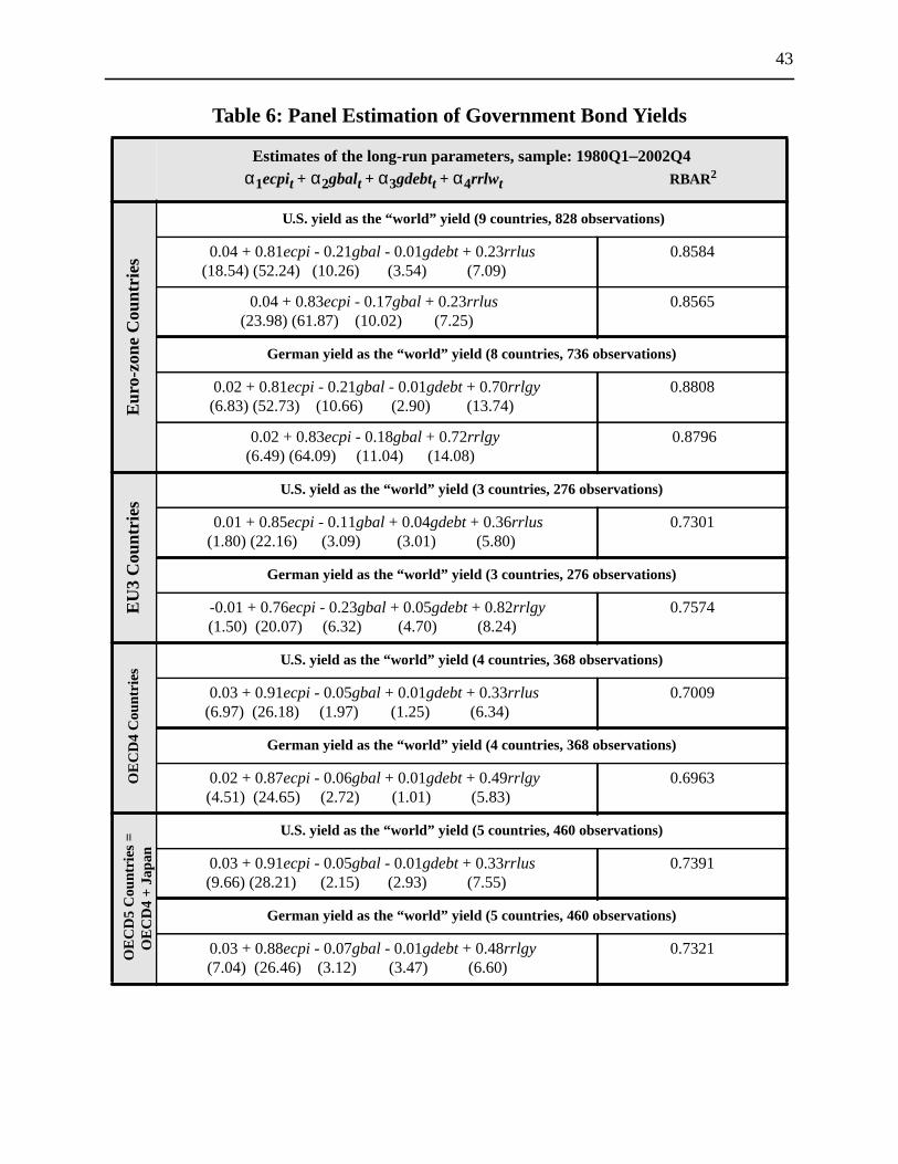
43

Table 6: Panel Estimation of Government Bond Yields

Estimates of the long-run parameters, sample: 1980Q1–2002Q4 α1ecpit + α2gbalt + α3gdebtt + α4rrlw t RBAR2

Eur

o-zo

ne C

ount

ries

U.S. yield as the “world” yield (9 countries, 828 observations)

0.04 + 0.81ecpi - 0.21gbal - 0.01gdebt + 0.23rrlus(18.54) (52.24) (10.26) (3.54) (7.09)

0.8584

0.04 + 0.83ecpi - 0.17gbal + 0.23rrlus (23.98) (61.87) (10.02) (7.25)

0.8565

German yield as the “world” yield (8 countries, 736 observations)

0.02 + 0.81ecpi - 0.21gbal - 0.01gdebt + 0.70rrlgy (6.83) (52.73) (10.66) (2.90) (13.74)

0.8808

0.02 + 0.83ecpi - 0.18gbal + 0.72rrlgy(6.49) (64.09) (11.04) (14.08)

0.8796

EU

3 C

ount

ries


0.01 + 0.85ecpi - 0.11gbal + 0.04gdebt+ 0.36rrlus(1.80) (22.16) (3.09) (3.01) (5.80)

0.7301


-0.01 + 0.76ecpi - 0.23gbal + 0.05gdebt + 0.82rrlgy(1.50) (20.07) (6.32) (4.70) (8.24)

0.7574

OE

CD

4 C

ount

ries


0.03 + 0.91ecpi - 0.05gbal + 0.01gdebt + 0.33rrlus(6.97) (26.18) (1.97) (1.25) (6.34)

0.7009


0.02 + 0.87ecpi - 0.06gbal + 0.01gdebt + 0.49rrlgy(4.51) (24.65) (2.72) (1.01) (5.83)

0.6963

OE

CD

5 C

ount

ries

=O

EC

D4

+ J

apan



0.7391


0.03 + 0.88ecpi - 0.07gbal - 0.01gdebt + 0.48rrlgy(7.04) (26.46) (3.12) (3.47) (6.60)

0.7321

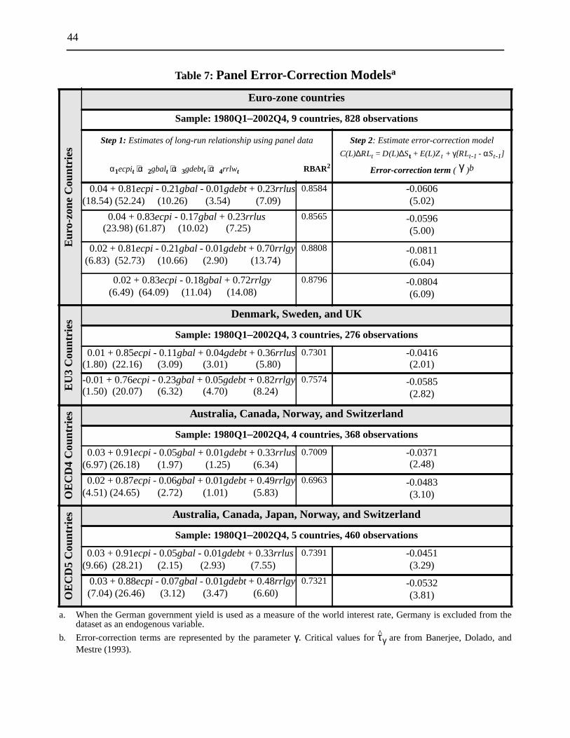
44

d from the

nd

Table 7: Panel Error-Correction Modelsa

a. When the German government yield is used as a measure of the world interest rate, Germany is excludedataset as an endogenous variable.

Eur

o-zo

ne C

ount

ries

Euro-zone countries

Sample: 1980Q1–2002Q4, 9 countries, 828 observations

Step 1: Estimates of long-run relationship using panel data

α1ecpit + α2gbalt + α3gdebtt + α4rrlw t RBAR2

Step 2: Estimate error-correction model

C(L)∆RLt = D(L)∆St + E(L)Zt + γ[RLt-1 - αSt-1]

Error-correction term ( γ )b

b. Error-correction terms are represented by the parameterγ. Critical values forτγ are from Banerjee, Dolado, aMestre (1993).

0.04 + 0.81ecpi- 0.21gbal - 0.01gdebt+ 0.23rrlus(18.54) (52.24) (10.26) (3.54) (7.09)

0.8584 -0.0606(5.02)

0.04 + 0.83ecpi - 0.17gbal + 0.23rrlus(23.98) (61.87) (10.02) (7.25)

0.8565 -0.0596(5.00)

0.02 + 0.81ecpi- 0.21gbal - 0.01gdebt+ 0.70rrlgy (6.83) (52.73) (10.66) (2.90) (13.74)

0.8808 -0.0811(6.04)

0.02 + 0.83ecpi - 0.18gbal + 0.72rrlgy (6.49) (64.09) (11.04) (14.08)

0.8796 -0.0804(6.09)

EU

3 C

ount

ries Denmark, Sweden, and UK


0.01 + 0.85ecpi- 0.11gbal+ 0.04gdebt+ 0.36rrlus(1.80) (22.16) (3.09) (3.01) (5.80)

0.7301 -0.0416(2.01)

-0.01 + 0.76ecpi- 0.23gbal+ 0.05gdebt+ 0.82rrlgy(1.50) (20.07) (6.32) (4.70) (8.24)

0.7574 -0.0585(2.82)

OE

CD

4 C

ount

ries Australia, Canada, Norway, and Switzerland


0.03 + 0.91ecpi- 0.05gbal+ 0.01gdebt+ 0.33rrlus(6.97) (26.18) (1.97) (1.25) (6.34)

0.7009 -0.0371(2.48)

0.02 + 0.87ecpi- 0.06gbal+ 0.01gdebt+ 0.49rrlgy(4.51) (24.65) (2.72) (1.01) (5.83)

0.6963 -0.0483(3.10)

OE

CD

5 C

ount

ries Australia, Canada, Japan, Norway, and Switzerland


0.03 + 0.91ecpi- 0.05gbal - 0.01gdebt + 0.33rrlus(9.66) (28.21) (2.15) (2.93) (7.55)

0.7391 -0.0451(3.29)

0.03 + 0.88ecpi- 0.07gbal - 0.01gdebt+ 0.48rrlgy (7.04) (26.46) (3.12) (3.47) (6.60)

0.7321 -0.0532(3.81)

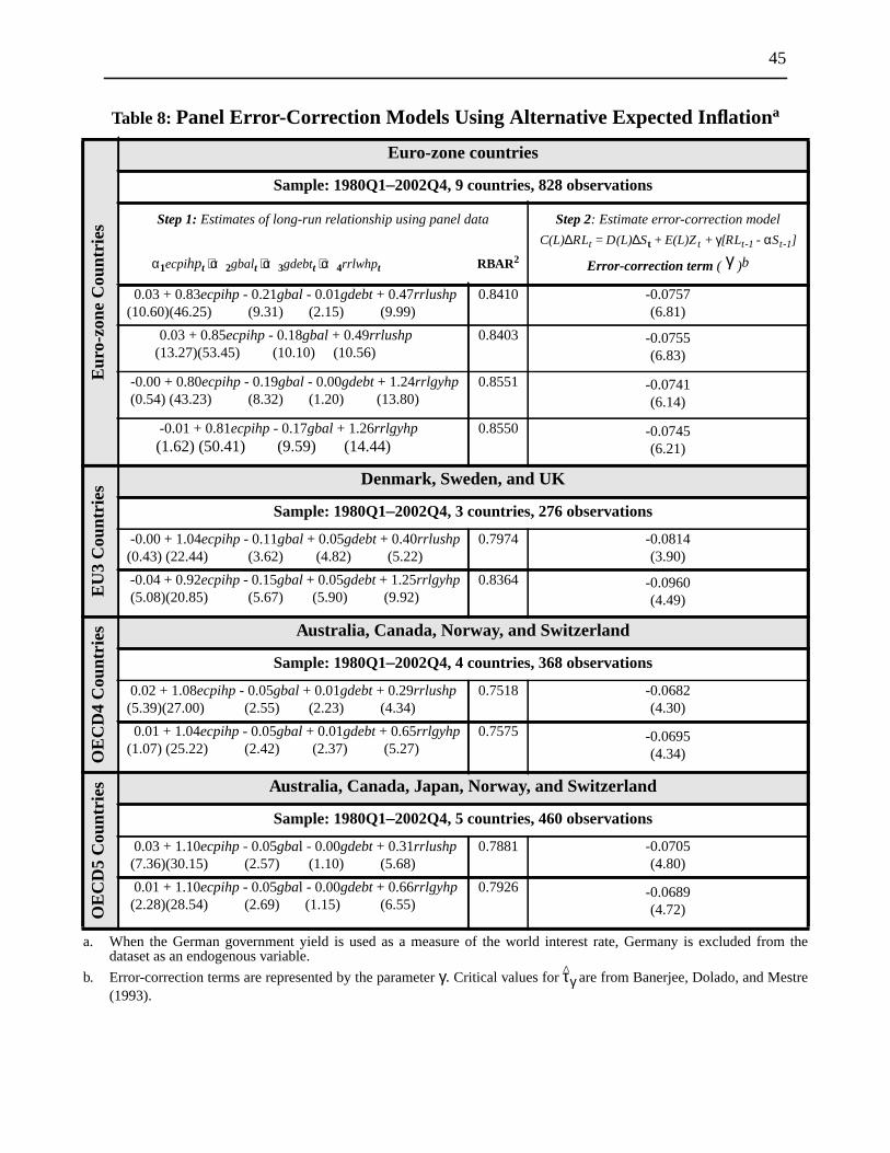
45

a. d from the

b. stre

Table 8: Panel Error-Correction Models Using Alternative Expected Inflationa

When the German government yield is used as a measure of the world interest rate, Germany is excludedataset as an endogenous variable.

Eur

o-zo

ne C

ount

ries

Euro-zone countries


Step 1: Estimates of long-run relationship using panel data

α1ecpihpt + α2gbalt + α3gdebtt + α4rrlwhpt RBAR2

Step 2: Estimate error-correction model

C(L)∆RLt = D(L)∆St + E(L)Zt + γ[RLt-1 - αSt-1]

Error-correction term ( γ )b

Error-correction terms are represented by the parameterγ. Critical values forτγ are from Banerjee, Dolado, and Me(1993).

0.03 + 0.83ecpihp - 0.21gbal - 0.01gdebt + 0.47rrlushp(10.60)(46.25) (9.31) (2.15) (9.99)

0.8410 -0.0757(6.81)

0.03 + 0.85ecpihp - 0.18gbal + 0.49rrlushp(13.27)(53.45) (10.10) (10.56)

0.8403 -0.0755(6.83)

-0.00 + 0.80ecpihp - 0.19gbal - 0.00gdebt + 1.24rrlgyhp (0.54) (43.23) (8.32) (1.20) (13.80)

0.8551 -0.0741(6.14)

-0.01 + 0.81ecpihp - 0.17gbal + 1.26rrlgyhp(1.62) (50.41) (9.59) (14.44)

0.8550 -0.0745(6.21)

EU

3 C

ount

ries Denmark, Sweden, and UK


-0.00 + 1.04ecpihp- 0.11gbal+ 0.05gdebt+ 0.40rrlushp(0.43) (22.44) (3.62) (4.82) (5.22)

0.7974 -0.0814(3.90)

-0.04 + 0.92ecpihp- 0.15gbal+ 0.05gdebt+ 1.25rrlgyhp (5.08)(20.85) (5.67) (5.90) (9.92)

0.8364 -0.0960(4.49)

OE

CD

4 C

ount

ries Australia, Canada, Norway, and Switzerland


0.02 + 1.08ecpihp - 0.05gbal + 0.01gdebt + 0.29rrlushp(5.39)(27.00) (2.55) (2.23) (4.34)

0.7518 -0.0682(4.30)

0.01 + 1.04ecpihp- 0.05gbal+ 0.01gdebt+ 0.65rrlgyhp(1.07) (25.22) (2.42) (2.37) (5.27)

0.7575 -0.0695(4.34)

OE

CD

5 C

ount

ries Australia, Canada, Japan, Norway, and Switzerland


0.03 + 1.10ecpihp - 0.05gbal - 0.00gdebt+ 0.31rrlushp (7.36)(30.15) (2.57) (1.10) (5.68)

0.7881 -0.0705(4.80)

0.01 + 1.10ecpihp - 0.05gbal - 0.00gdebt+ 0.66rrlgyhp (2.28)(28.54) (2.69) (1.15) (6.55)

0.7926 -0.0689(4.72)

46

from the

from the

0

Table 9: Panel Estimation of Government Bond Yields Including Ireland


Euro zone excluding Ireland, 9 countries, 648 observationsa

a. When the German government yield is used as a measure of the world interest rate, Germany is excludedsample, leaving data for eight countries and 576 observations.

0.03 + 1.01ecpi - 0.18gbal - 0.01gdebt + 0.31rrlus (11.42) (42.57) (7.70) (3.21) (5.64)

0.8271


0.8620

Euro zone including Ireland, 10 countries, 720 observationsb

b. When the German government yield is used as a measure of the world interest rate, Germany is excludedsample, leaving data for nine countries and 648 observations.


0.8100


0.8463

Table 10: Fixed-Effect Panel Estimation of Government Bond Yields

Eur

o-zo

ne C

ount

ries




0.8126

Fixed-country effects: AT: -0.005, BG: -0.005, FN: 0.013, FR: 0.002, GY: -0.003, IT: -0.010, NT: -0.004, PT: 0.011, SP: 0.00


-0.005 + 0.84ecpi - 0.28gbal + 0.02gdebt + 0.75rrlgy (1.00) (44.06) (13.75) (4.37) (15.67)

0.8576

Fixed-country effects: AT: -0.001, BG: -0.015, FN: 0.021, FR: 0.007, IT: -0.021, NT: -0.002, PT: 0.010, SP: 0.002

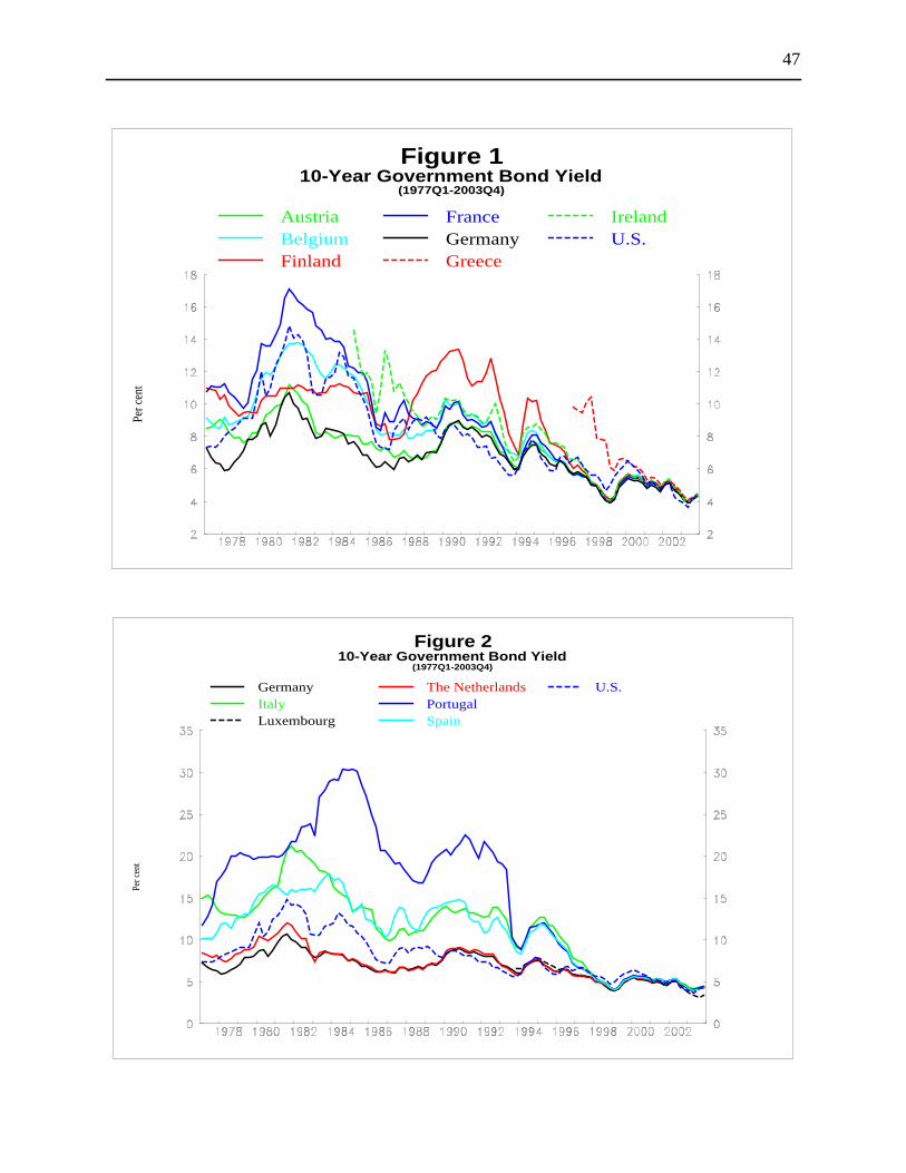
47

AustriaBelgiumFinland

FranceGermanyGreece

IrelandU.S.

Figure 110-Year Government Bond Yield

(1977Q1-2003Q4)

Per

cen

t

GermanyItalyLuxembourg

The NetherlandsPortugalSpain

U.S.


(1977Q1-2003Q4)

Per

cen

t

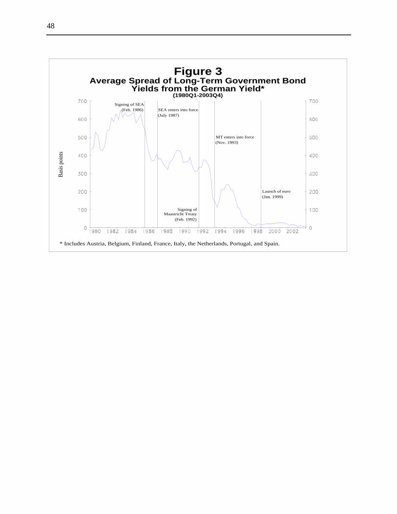
48

Signing of SEA(Feb. 1986) SEA enters into force

(July 1987)

Signing ofMaastricht Treaty

(Feb. 1992)

MT enters into force(Nov. 1993)

Launch of euro(Jan. 1999)

Figure 3Average Spread of Long-Term Government Bond

Yields from the German Yield*(1980Q1-2003Q4)

Bas

is p

oint

s

* Includes Austria, Belgium, Finland, France, Italy, the Netherlands, Portugal, and Spain.

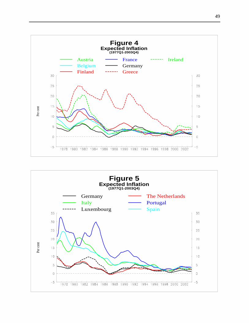
49


FranceGermanyGreece

Ireland

Figure 4Expected Inflation

(1977Q1-2003Q4)

Per

cen

t




(1977Q1-2003Q4)

Per

cen

t

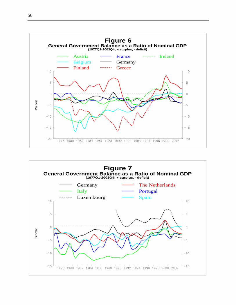
50


FranceGermanyGreece

Ireland

Figure 6General Government Balance as a Ratio of Nominal GDP

(1977Q1-2003Q4; + surplus, - deficit)

Per

cen

t





Per

cen

t

51


FranceGermanyGreece

Ireland

Figure 8General Government Debt as a Ratio of Nominal GDP

(1977Q1-2003Q4)

Per

cen

t




(1977Q1-2003Q4)

Per

cen

t

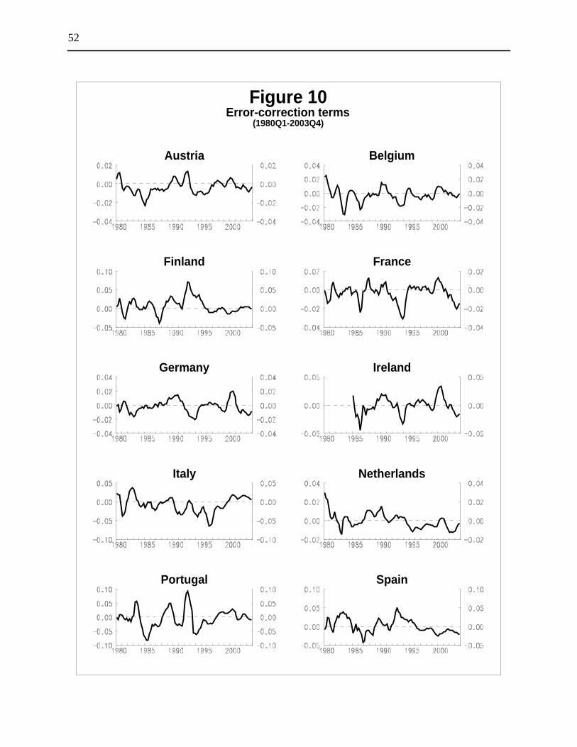
52

Figure 10Error-correction terms

(1980Q1-2003Q4)

Austria Belgium

Finland France

Germany Ireland

Italy Netherlands

Portugal Spain

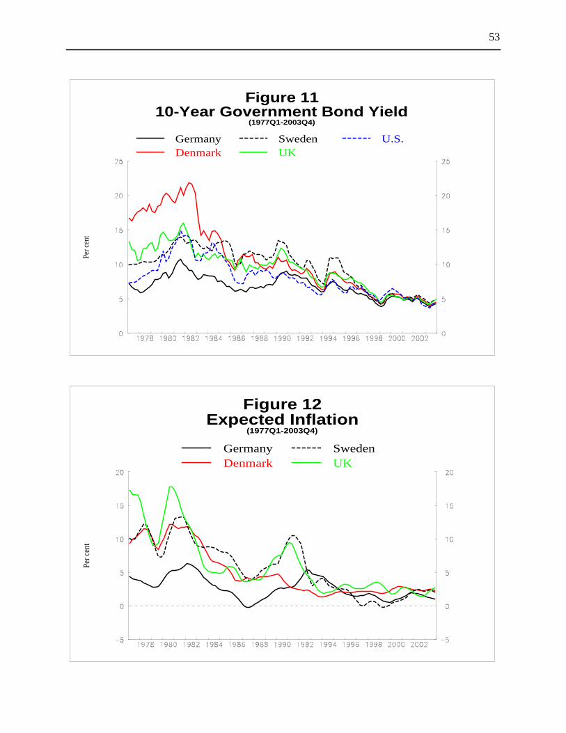
53

GermanyDenmark

SwedenUK

U.S.


(1977Q1-2003Q4)

Per

cen

t

GermanyDenmark

SwedenUK


(1977Q1-2003Q4)

Per

cen

t

54

GermanyDenmark

SwedenUK



Per

cen

t

GermanyDenmark

SwedenUK


(1977Q1-2003Q4)

Per

cen

t

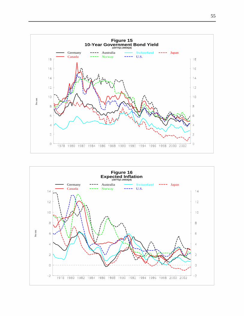
55

GermanyCanada

AustraliaNorway

SwitzerlandU.S.

Japan


(1977Q1-2003Q4)

Per

cen

t

GermanyCanada

AustraliaNorway

SwitzerlandU.S.

Japan


(1977Q1-2003Q4)

Per

cen

t

56

GermanyCanada

AustraliaNorway

SwitzerlandU.S.

Japan



Per

cen

t

GermanyCanada

AustraliaNorway

SwitzerlandU.S.

Japan


(1977Q1-2003Q4)

Per

cen

t

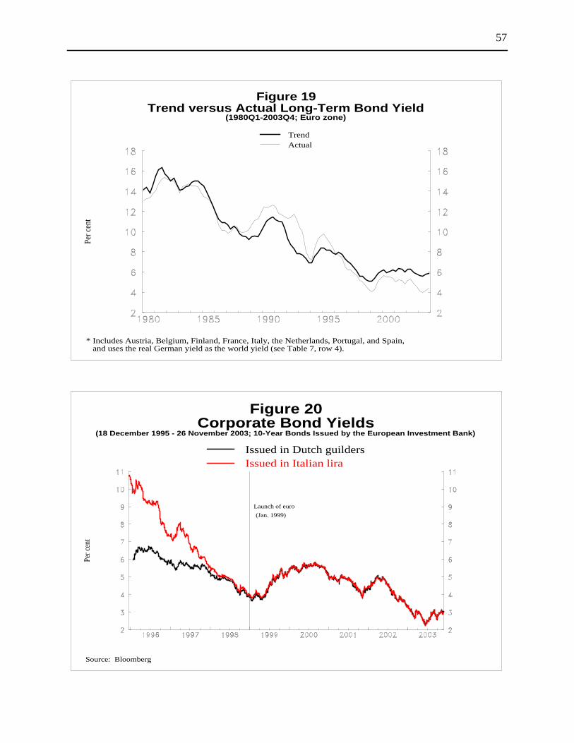
57

TrendActual

Figure 19Trend versus Actual Long-Term Bond Yield

(1980Q1-2003Q4; Euro zone)

Per

cen

t

* Includes Austria, Belgium, Finland, France, Italy, the Netherlands, Portugal, and Spain, and uses the real German yield as the world yield (see Table 7, row 4).

Launch of euro

(Jan. 1999)

Issued in Dutch guildersIssued in Italian lira

Figure 20Corporate Bond Yields

(18 December 1995 - 26 November 2003; 10-Year Bonds Issued by the European Investment Bank)

Per

cen

t

Source: Bloomberg

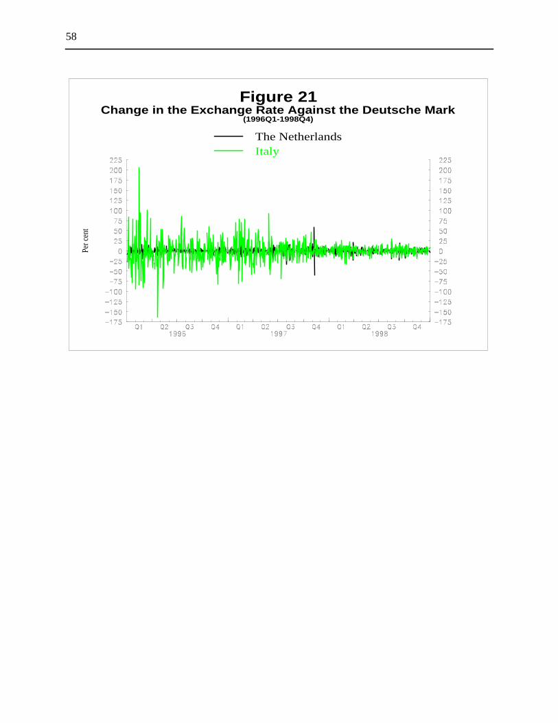
58

The NetherlandsItaly

Figure 21Change in the Exchange Rate Against the Deutsche Mark

(1996Q1-1998Q4)

Per

cen

t

Bank of Canada Working PapersDocuments de travail de la Banque du Canada

Working papers are generally published in the language of the author, with an abstract in both officiallanguages.Les documents de travail sont publiés généralement dans la langue utilisée par les auteurs; ils sontcependant précédés d’un résumé bilingue.

Copies and a complete list of working papers are available from:Pour obtenir des exemplaires et une liste complète des documents de travail, prière de s’adresser à:

Publications Distribution, Bank of Canada Diffusion des publications, Banque du Canada234 Wellington Street, Ottawa, Ontario K1A 0G9 234, rue Wellington, Ottawa (Ontario) K1A 0G9E-mail: [email protected] Adresse électronique : [email protected] site: http://www.bankofcanada.ca Site Web : http://www.banqueducanada.ca

20042004-22 Financial Conditions Indexes for Canada C. Gauthier, C. Graham, and Y. Liu

2004-21 Exchange Rate Pass-Through and the Inflation Environmentin Industrialized Countries: An Empirical Investigation J. Bailliu and E. Fujii

2004-20 Commodity-Linked Bonds: A Potential Means forLess-Developed Countries to Raise Foreign Capital J. Atta-Mensah

2004-19 Translog ou Cobb-Douglas? Le rôle des duréesd’utilisation des facteurs E. Heyer, F. Pelgrin and A. Sylvain

2004-18 When Bad Things Happen to Good Banks:Contagious Bank Runs and Currency Crises R. Solomon

2004-17 International Cross-Listing and the Bonding Hypothesis M. King and D. Segal

2004-16 The Effect of Economic News on Bond Market Liquidity C. D’Souza and C. Gaa

2004-15 The Bank of Canada’s Business OutlookSurvey: An Assessment M. Martin and C. Papile

2004-14 National Saving–Investment Dynamics andInternational Capital Mobility F. Pelgrin and S. Schich

2004-13 Contraintes de liquidité et capital humaindans une petite économie ouverte F. Pelgrin

2004-12 Durées d’utilisation des facteurs et fonction deproduction : une estimation par la méthode desmoments généralisés en système E. Heyer, F. Pelgrin, and A. Sylvain

2004-11 Estimating New Keynesian Phillips CurvesUsing Exact Methods L. Khalaf and M. Kichian

2004-10 Public Venture Capital and Entrepreneurship O. Secrieru and M. Vigneault

2004-9 Estimating Policy-Neutral Interest Rates for CanadaUsing a Dynamic Stochastic General-EquilibriumFramework J.-P. Lam and G. Tkacz

2004-8 The Economic Theory of Retail Pricing: A Survey O. Secrieru

2004-7 The Demand for Money in a Stochastic Environment J. Atta-Mensah