BIT33 (1993). 137-150.

C O N V E R G E N C E O F A C L A S S O F R U N G E - K U T T A

M E T H O D S F O R D I F F E R E N T I A L - A L G E B R A I C

S Y S T E M S O F I N D E X 2

LAURENT JAY

Universit~ de Gen~ve, D~partement de math~matiques, Rue du Li~vre 2-4, Case postale 240, CH-1211 Gen~ve 24, Switzerland.

e-mail: jay@c#euge51.bitnet or: jay@uni2a.unioe.ch.

Abstract.

This paper deals with convergence results for a special class of Runge-Kutta (RK) methods as applied to differential-algebraic equations (DAE's) of index 2 in Hessenberg form. The considered methods are stiffly accurate, with a singular RK matrix whose first row vanishes, but which possesses a nonsingular submatrix. Under certain hypotheses, global superconvergence tbr the differential components is shown, so that a conjecture related to the Lobano IliA schemes is proved. Extensions of the presented results to projected RK methods are discussed. Some numerical examples in line with the theoretical results are included.

Subject classifications: AMS(MOS): 65L06.

Key words: Differential-algebraic, index 2, initial value problems, Runge-Kutta methods.

1. Introduction.

Differential-algebraic equations (DAE's) of index 2 arise in many applications, such as in mechanical modelling of constrained systems (see [4, pp. 6-7] or [5, pp. 483-486 & 539-540]). Whereas optimal convergence results for Runge-Kutta (RK) methods with an invertible RK matrix are well-known (see I-4, Section 4] and [5, Section VI.7]), this paper is concerned only with RK methods having a singular RK matrix.

The main result of this article (Theorem 5.2 below) proves a conjecture (see [4, pp. 18, 46 & 47] and 1-5, p. 515]) related to the Lobatto IliA processes which belong to the class of methods considered in this paper (see Section 2). Its proof necessitates several preliminary results which are collected in Section 3 (properties of the RK coefficients), in Section 4 (existence, uniqueness of the numerical solution, and influence of perturbations), and in Section 5 (estimates of the local error and

Received June 1991. Revised May 1992.

138 LAURENT JAY convergence). Extensions of the previous results to projected RK methods are discussed in Section 6. Finally, some numerical experiments are given in Section 7 which illustrate the theoretical results. Let us mention that all the results presented in this paper remain valid for some other types of DAE's (for further details see [4, pp. 5 & 30]).

In this report, we consider the following system of DAE's given in an autonomous and semi-explicit formulation (or Hessenberg form)

y' = f (y ,z) , y(xo) = yosN" , (1.1)

0 = g(y), z(xo) = Zo e R"

where the initial values (Yo, zo) are assumed to be consistent, i.e.,

(1.2) O(Yo) = O, (orf)(Yo, Zo) = O.

We suppose that f and 9 are sufficiently differentiable and that

(1.3) (9yf~)(Y,Z) is invertible

in a neighbourhood of the exact solution (index 2).

2. The class of Runge-Kutta methods.

One step of an s-stage Runge-Kutta (RK) method applied to (1.1) reads (see [3], [4, p. 30] or [5, p. 502])

(2.1a) Yl = Yo + ~ biki, z~ = Zo + i bil, i = 1 i = 1

where

(2.1b) k~ = l f ( Y , Z , ) , 0 = g(Y3

and the internal stages are given by

(2.1c) r, = yo + o,,k,, z , = zo + a , / , . j=1 j=1

For a RK method we denote A : = (ai,)i., the RK matrix, b: = (bl,..., b~) r the weight vector, and c := (el ..... c,) r : = A~, the node vector where ~ : = (I ..... 1) r. Let B(p), C(q), D(r) be the following simplifyin9 assumptions which are related to the construc- tion of such methods

B(p): i bic~-t = 1/k k = 1, . . . ,p; i = 1

C(q): ~ a, ,c~-l= 4 /k i = 1 . . . . . s, k = l, . . . ,q; j = l

C O N V E R G E N C E O F A C L A S S O F R U N G E - K U T T A M E T H O D S . . . 139

D(r): ~ k-1 bic i aij = bj(1 - ck)/k j = 1,. . . , s, k = 1,. . . , r. i = 1

Throughout this paper we are only interested in RK methods with s _> 2 and coefficients satisfying the hypotheses

H l : a l j = 0 f o r j = 1 . . . . . s;

H2: the submatrix ,4 := (ai~)i.~ ~ 2 is invertible;

H3: bl = a,i for i = 1 . . . . . s, i.e., the method is stiffly accurate.

For these methods, the lj in (2.1) are not well-defined, but in order to define y ~ and z 1, it is sufficient to solve the equivalent nonlinear system (4.2) below and to apply the fourth remark hereafter.

REMARKS. The following results can be easily proven. 1) The definition of c coincides with the condition C(1). 2) H3 together with the condition B(1) leads to Cs = 1. If in addition C(q) (resp. D(r))

is satisfied then B(q) (resp. B(r + 1)) holds.

3) From H t it follows that cl = 0, Y1 = Yo, g(Y0 = g(Yo) = 0, ZI = zoin(2.1), and that A is singular.

4) H3 implies that Yl = Y~, g(Yl) = g(Y~) = 0, and zl = Zs in (2.1).

A main advantage of methods verifying H1 and H3 is that the first stage of one step is equal to the last stage of the previous step which coincides with the current initial value, so that it requires no supplementary computation. The most prominent examples of such methods are given by collocation methods like the Lobatto IliA schemes whose coefficients c~ = 0, c2, . . . , c, = 1 are the zeros of the polynomial of degree s

ds--2 (2.2) dx~- 2 (xS- l (x - 1) s - l )

and which fulfil the conditions B(2s -- 2), C(s), and D(s - 2). Due to their symmetry, they are often used for the solution of boundary value problems (see [2]).

3. Properties of Runge-Kutta coefficients.

This section deals with relations of the RK coefficients appearing in the demon- stration of Theorem 4.4.

THEOREM 3.1. Suppose that the hypotheses H1, H2 and H3 are satisfied together with the condition D(r). For a f i x ed p ~ ~\{0}, consider a multi-index v = (vl . . . . . vp) satisfying vi >_ 1 and let ~ >_ O. Iftvl := ~ = ~ vi <_ r then we have

140 LAURENT JAY

(3.1) er_,c" M, A1 = e r - , C ' M I . . . M o A , = 0

where we have set

(3.2) C : = diag(e2, . . . , cs), AI: = (a21 . . . . . a~l) T, es_ 1: = (0 , . . . , 0 , 1) r.

The matrices Mi are of the form A*~, C *~ or AC~'*A-* and it is supposed that M. = cvG -1.

REMARK. Wi thou t loss of generality p _< r can be assumed.

PROOF. In matr ix notat ion, the simplifying assumption D(r) becomes

(3.3a) f fTck-*A = k l ( g T __ gT~k) k = 1,... ,r,

(3.3b) /TTCk- t ~ = k - l b , k = 1 . . . . . r

where if: = (bz,.. . , b~) T, and H3 reads

(3.4a) /~r = e T_ 1A

(3.4b) bl = e T_ 1A1 = a~,.

Mult iplying (3.3a) with .4- * and using/TTA - 1 = e T_ 1 which follows from (3.4a), we

obtain

(3.5) f f r t~k~ 1 = e T , -- kF)Tdk-'; k = 1,... ,r.

Repeated applicat ion of (3.3a), (3.4a), and (3.5) to (3.1) shows that this expression is a linear combina t ion of terms/~rCr,~- *A1 with 1 _< 7 -< r. They all vanish because of

(3.6) ffTC~A-*A, = eT_IA1 -- ?bTC~-tA1 = bl - bl = 0

which is a consequence of (3.5), (3.4b), and (3.3b). []

LEMMA 3.2. Suppose that the hypotheses H1, H2, and H3 hold. Then R(z), the

stability function of the method, satisfies at

= - e , _ , A A,. (3.7) R ( ~ ) T - - 1 ~

PROOF. R(z) is the numerical solution after one step of the me thod applied to the

test equat ion

(3.8) y' = 2y, Yo = 1,

with z : = h2. By using H3 we get R(z)= y, = Y~ = e f ( I~- zA)-*~. The result

follows from

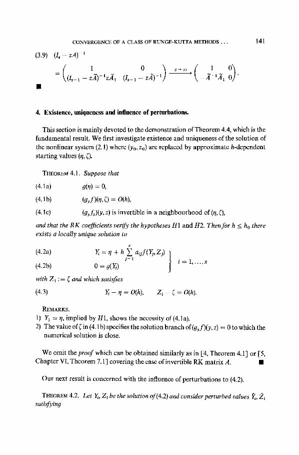
(3.9)

CONVERGENCE OF A CLASS OF RUNGE-KUTTA M E T H O D S . . .

(I~ - z A ) - 1

( o = (l~-I - zA)-lzAl (I~-1 -- z/l) -1 ) - A - 1 A 1 "

141

4. Existence, uniqueness and influence of perturbations.

This section is mainly devoted to the demonstration of Theorem 4.4, which is the fundamental result. We first investigate existence and uniqueness of the solution of the nonlinear system (2.1) where (Yo, z0) are replaced by approximate h-dependent starting values (~, 0.

THEOREM 4.1. Suppose that

(4. la) g(q) = O,

(4. lb) (g,f)(t h () = O(h),

(4. lc) (gff~)(y, z) is invertible in a neighbourhood of (q, 0,

and that the RK coefficients verify the hypotheses H1 and H2. Then for h <_ ho there exists a locally unique solution to

(4.2a) Yi = q + h ~ aJ'(Yj, Zi) / j = l / i = 1, . ,s

(4. 25) 0 = g(Y~) "" J

with Z 1 := ~ and which satisfies

(4.3) Y~ - I? = O(h), Z , - ( = O(h).

REMARKS.

1) Y1 = q, implied by H1, shows the necessity of(4.1a). 2) The value of ( in (4. lb) specifies the solution branch of(gyf)(y, z) = 0 to which the

numerical solution is close.

We omit the proof which can be obtained similarly as in [4, Theorem 4.1] or [5, Chapter VI, Theorem 7.1] covering the case of invertible RK matrix A. •

Our next result is concerned with the influence of perturbations to (4.2).

THEOREM 4.2. Let Yi, Zi be the solution of(4.2) and consider perturbed values ~, Zi satisfying

142 LAURENT JAY

(4.4a) ~ = fl + h ~ aij f(~,2j) + h61 j = l

(4,4b) 0 = g(~) + 01 i = 1 , . . . , s

with Z1 := ~. In addition to the assumptions of Theorem 4.1, suppose that

(4.5) 0 - r t - - O ( h ) , 2~ - ( = O(h), 3i = O(h), Oi = O(h2).

Then we have for h <_ ho the estimates

(4.6a) II~ - Y~II -< C(ll~ - rttl + h 2 II~ - (11 + h 11611 + II011),

(4.6b) 112~ - Z, It < h ( h I1~ - rttl + h II( - ~ll + h 11611 + HOII)

where 6 = (31 . . . . . 6,) r, 116 I1 = max~ II6~tl and similarly for O.

REMARKS.

1) The condit ions (4.5) ensure that all terms O(-) in the p roof below are small. 2) The terms containing ~ - ( will be computed in detail. This will be justified in the

demons t ra t ion of Theorem 4.4. 3) We introduce the nota t ion Art = ~ -- rt, A( = ~ - (, Y = (Y1,--., Ys) T,

A Y = Y - Y,, ilAIql = maxi IlAY/ll and similarly for the z-component . Over a mult iple-vector a tilde ' ~ ' indicates the removal of its first subvector, e.g.,

~" = (Y2 . . . . . y~)r.

PROOF. H1 implies that Y1 -- rt and 1~] = 0 + h61. Therefore we have

(4.7) AY1 = Art + h61, AZ~ = A(

which proves the s tatement (4.6) for i = 1. Hence from (4.2b) and (4.4b) we deduce

that

(4.8) gr(rt)Art = O(h IIArtll + h IIb~[t + II0~ll).

Fo r i >_ 2, by subtract ing (4.2) f rom (4.4) we obtain by l inearization

(4.9a) AYi = Art + h i aiJfr(YJ, ZJ)AY~ + h ~ aljf~(~,Z~)AZ i j = l j = l

+ hfi + O(h NAYII 2 + h ItAYI[ " tIAZII + h IIAZtI2),

(4.9b) 0 = gr(Y/)AY/+ Oi + O(HAY/[]2) •

It can be noticed that if fzz = 0 ( f linear in z) the expression O(h IIAZII 2) in (4.9a) disappears, but O(h IIAY[I " IIAZII) remains. Therefore we retain all terms permitt ing to analyse easily this si tuation (see the first remark after Theorem 4.4). By using tensor notat ion, (4.9) can be rewrit ten with the help of (4.7) as

(4.10a)

(4.10b)

where

(4.11a)

(4. l ib)

(4.1 lc)

C O N V E R G E N C E O F A C L A S S O F R U N G E - K U T T A M E T H O D S . . .

AY = ls-~ ® Aq + h(A® I.){fr}AY + A~ ® (fz(q, 0hA0

+ (sl ® I,,){fz}haZ + hS+ O(h I IA~' I I 2 + h I IAYI I • I IAZI I

+ h IIAZll 2 + h IIAnlI + h 2 I1,$~1t),

0 = {O~,}AY + O + O(IIA?II 2)

{fy): = blockdiag(L(Y2, Z2) . . . . . f~(Y~, Zs)),

{f~} : = blockdiag (fz(Yz, Z2),..., f~(Y~, Zs)),

(gy} := blockdiag (gy(Yz),..., gy(Y~)).

143

Insertion of the expression (4.10a) into (4.10b) yields

(4.12) - {gr}(/l ® I,){f~}hk2~ =

{gr}(~s_l ® A~/+ h(/l ® I,){J~}AY + A1 ® (fz(q, 0hA0 + h~)

+ i f + O(t la?l l 2 + h IIA?It" tlAZtt + h ttAZtt 2 + h llA~#tl + h 2 lt,hlt).

In view of (4.3) we have

(4.13) gr(Yi)aufz(Ys, ZS) = au(grf~)(rl, 0 + O(h),

thus the left matrix of (4.12) can be written as

(4.14) {gy}(/~ @ I,,){f:} = /T ® (gyf=)(r#, 0 + O(h)

and is invertible by H2 and (4. lc) ifh is sufficiently small. Hence from (4.12), and by the use of (4.8) for (4.15'), we get

(4.15) hAZ = - ( {g r } (A ® I , ) { f : } ) - l{gy}

x ( l , - t ® At/+ h(/l® I,){fy}AY + / l l ® (fz(##, 0hA0

+ O(IIA~II 2 + h tlA?II • IIAZtl + h tlA~tl 2 + h IIAnll

+ h IIA~II 2 + h 2 II<$11t + h tl3"II + I1#II)

(4.15') = -({gr)(A ® I,,){f:})- ' {gr}(/T, @ (f~(q, 0hA0)

+ O(h tta?tl + h IIA2112 + h tlAnll + h ItAffll 2 + h If,51t + ll0N).

(4.15) inserted into (4.10a) leads to

(4.16) A~-= P.7(l~-x ® A~/+ h(,4 ® I,){fr}AY + A~ ® (f~(~/, 0hA0)

+ O(tlA?II 2 + h tlA?II" tlAZII + h tlA2tl 2 + h IIAr#ll

+ h IIA(tl 2 + h 2 I1,$~II + h IID"ll + IIOII),

with the following definitions

144 LAURENT JAY

(4.17) P X : = I(~_~), - F~(GyF~)-IGr, F ~ : = (A®I.){ fz}( f t®I , , , ) 1, G y : = {gy}.

W e p u t F~, o : = I s - 1 ® f~(r/, () a n d s ince the p r o j e c t o r P.i satisfies P.iF~ = 0, the t e r m inc lud ing A( in (4.16) can be expres sed as

(4.18) P~7(/T, ® (f~(q, 0 h A 0 ) = -P~(F~ -- F~,o)(.41 ® hA() = O(h 2 I[A(tl)

b e c a u s e o f / ' ~ - F~. o = O(h). •

LEMMA 4.3. In addition to the hypotheses of Theorem 4.1, suppose that the condi- tion C(q) holds and that (gyf)(r/, 0 = O(h~) with tc >_ t. Then the solution of(4.2), Y~, Zi,

satisfies

c"h m (4.19a) Y~ = t / + ~ D Y m ( q ) + O(h~+t),

m = l m.

(4.19b) Z~ = ((q) + ~ - - ~ . D Z , ( r l ) + O(h "+~)

where ~(rl) is defined by the condition (gyf) ( t / ,~( t / ) )= O, 2 = m i n ( x + 1,q), /~ = min(~c - t, q - 1) and D Y,,, DZ, are functions composed by derivatives o f f and g evaluated at (rh ((vl)).

PROOF. By the impl ic i t func t ion t h e o r e m we o b t a i n ((r/) - ( = O(h~). W e define

(y(x), z(x)) the so lu t ion of (1.1) wh ich satisfies y(xo) = ~ /and Z(Xo) = ((~/). T h e exac t

so lu t ion values ~ = ~ / = y(xo), ~ = ~(~) = z(xo), ~ = y(xo + cih), Zi = z(xo + c~h) satisfy (4.4) w i th 0i = 0 a n d

(4.20) 6i q! y ~ O ) \ q + 1 s=a

T h e d i f ference f r o m the n u m e r i c a l so lu t i on (4. 2) can thus be e s t i m a t e d wi th T h e o r e m

4.2, y ie ld ing

(4.21) II Y~ - y(xo + cih)ll = O(hmin(r+ 2"q+ l)), I lZi - Z(Xo "+- cih)l[ = O ( h m i n ( r ' q ) ) • •

THEOREM 4.4. In addition to the assumptions of Theorem 4.2, suppose that the conditions C(q), D(r) and the hypothesis H3 hold, and that (gyf)(rh 0 = O(h~) with

>__ 1. Then we have

(4.22a) ~ -- Y~ = P(r/, ~)(~ -- r/) + O(h 11,7 - ~11 + hm+2 II( - ~r[i + h H( - - ([I 2 + h H3[I + t101t),

(4.22b) Zs - Zs = R ( ~ ) ( ( - () + O(ll0 - r t l l + h It( - (11 + IlOll + IlOll/h)

where m = m i n 0c - 1, q - 1, r) _> 0, R is the stability function, and P is the projec- tor defined under the condition (1.3) by

(4.23) P : = I , - Q, Q : = f~(gyf=)- lgy.

CONVERGENCE OF A CLASS OF RUNGE-KUTTA METHODS . . . 145

REMARKS.

1) If the function f of (t. 1) is linear in z we have m = min(g, q, r). All terms O(h lt Af I[ 2) in the proof below can be replaced by O(h 3 liAr II 2) coming from the expression O(h tlAYII" IIAZII) of (4.16) (in this case the terms O(h IIAZII 2) and O(h IIAfll 2) are not present), so that (4.22a) becomes

(4.22a') ~ -- Y~ = P(r/, f)(tl - 1/)

+ O(h 114 - r/[I + hm+2 I1( - fll + ha I1( - (112 + h 11511 + tl011).

2) The important result consists in the factor h "+2 in front of I1( - fill in (4.22a)- (4.22a').

PROOF. We return to the end of the proof of Theorem 4.2 by taking Lemma 3.3 into account and using the same notations and definitions. According to (4.15') we have

(4.24) AZs = -e~r_x,zi-x.zixAf + O(IIAr/II + h IIAfII + 11511 + IlOll/h)

which together with formula (3.7) of Lemma 3.2 proves the statement (4.22b). (4.22a) remains to be proved. Taking (4.16), computing (I - hPz(.4 ® l ,){fr})- 1

by means of the series of yon Neumann, and using (4.18), we obtain

(y m--1 h~(P-4 ( -x~ ) (4.25) A ~ = P(~, 0A,1 - ( e r ~ N I,~) \~o.= ® I~){f,}) ~

x e.i(Fz - fz.o)(.4, ® hA() + O(h IIAt;ll + h m+2 IIA(II

+ h IIA(II 2 + h 2 115111 + h 115~11 + 11511),

With the help of Lemma 4.3, we will develop PX into h-powers. Let us first consider the expression

(4.26) GyFz = Is- 1 ® (gyf~)(tl, f(tt))

(1~-1 ® I , , + ~ h'+i(C'AC~,4 -1) ® D,i(r/)~ + O(h °'+t) X \ O<i+j_<to /

where o) = # (co = 2 if f is linear in z because j~(y, z) is independent of z), and the D~j are terms of the same type as the DY,,, and DZ, of Lemma 4.3. Using again the series of yon Neumann, we see that its inverse is of the form

(4.27) (GyFz) -1 = 1,-1 ® (vyf=)-l(r/,f(r/))

+ o<t~,+,al~" _<~, hl~'l+Iat(~C""4Ct~<4-t) ® E ' a ( r l ) + O ( h o + ~ ) \ , = l

where the E~a are expressions like the Do, ~ = (~x,-.., c%) and fl = (ill . . . . . flo,) are multi-indices in ~,o. Here the norm of a multi-index 7 = (71 . . . . . %0) is defined by

146 LAURENT JAY

t~[" = ~,~'= z "Y~- If we insert (G,F~)- 1 into the definition of P~ and develop G r and F~ in powers of h, we arrive at

(4.28) P~ = Is-1 ® P(~,((q))

+ ~ h I~I+N X C ~ ' d - l C ~' ®H~O/) + O(h ~+1) o <l~l+}v[_< co i

where H ~ are analogous to the D s. Further, x = ( tq, . . . , xo~) and v = ( ] J 1 . . . . , v,o) are multi-indices in NC

With these preparations we are now able to prove (4.22a) by developing into h-powers the expression including A~ in (4.25). For example we consider the term

which corresponds to 6 = 1 in the sum entering in (4.25)

(4.29) H : = --(eT_ ~ ® Im)hP~(A- ® I.){fy}P~(F~ - F~,o)(A1 ® hA().

As a consequence of (4.28) we obtain

(4.30a) H = h z ~ hl"l+l~l+Ncrw" K,,~(tl)A( n t- O ( h m+ 2 [[AfH) 1 _< I~1 +lvl +lvl < m'--- 1

where

(4.30b)

and the K~v, are other expressions like the Di j . Further, xj = (xjl . . . . . xjo), vj = (vj1,...,v.,o) (where j = 1,2) are multi-indices in N '°, and we also have

J ~: = (Kx, ~:2), I~1: = I~1 + Ix21, v = (vl , vz), I v l : = lvll + IVzl, z = (zi, z2) with z 2 strict- ly positive. The coefficients C~. are of the form (3.1) and by Theorem 3.1 they vanish by virtue oflxt + [vt + Izl + 1 < r. We thus get H = O(h" + 2 [[A([D. All other remain- ing terms can be treated in a similar way, so that the statement (4.22a) results. •

5. Local error and convergence.

Theorem 4.4 yields the main component for the convergence proof of RK methods with singular RK matrix A. The rest closely follows the proofs given in [4, Sections 4 & 5] and [5, Sections VI.7 & VI.8]. For convenience of the reader, we present here the final results and give only some indications for their proof. Details

are omitted. We consider one step of a RK method (2.1) with initial values ~1 = y(x), ( = z(x)

on the exact solution and we want to give estimates for the local error

(5.1) 6yh(X) = Yl -- y(x + h), &h(x) = zx -- z(x + h).

CONVERGENCE OF A CLASS OF RUNGE-KUTTA METHODS... 147

THEOREM 5.1. Assume that the R K coefficients satisfy the conditions B(p), C(q), and D(r), and that the hypotheses HI, H2, and H3 hold. Then we have

(5.2) 6yh(x ) = O(hmln(p'2q'q+r+l)+l), c~zh(x ) = O(hq).

REMARKS.

1) If the function f of (I.1) is linear in z then we get

(5.2') 6yh(x) = O(h '~i"(v" 20+ 1,o+,+ 1)+ 1).

2) p _> q follows from Remark 2) in Section 2.

The proof is omitted. The ideas and techniques are similar to those of [4, Lemma 4.3 & Theorem 5.9] and [5, Chapter VI, Lemma 7.4 & Theorem 8.10] which are devoted to the case of invertible RK matrix A. The local error of the y-component can be found by repeated application of simplifying assumptions to the order conditions. •

THEOREM 5.2. Consider the differential-algebraic system (1.1) of index 2 with consistent initial values and the R K method (2.1). In addition to the hypotheses of Theorem 5.1, suppose further that IR(~)t < 1 and q >_ 2 if R ( ~ ) = 1. Then for x, - Xo = nh <_ Const, the 91obal error satisfies

fO(h min(p'2q'q+r+l) if - 1 < R(oo) < 1, (5.3a) Y" - - Y ( X n ) = (O(h mln(p'2q- l'q+r+ l)) if R(oo) = 1,

(5.3b) z, - z(x,) = ~ O(hq) if - 1 < R(oo) < 1, (O(h o-1) if R ( ~ ) = 1.

REMARKS.

1) If the function f of (1.1) is linear in z then we have

~O(h min~'2a+l"q+r+I)) if - 1 _< R(oo) < 1, (5.3a') Y" - - y ( X n ) = (O(h min(''2q'q+r+ l)) if R(oo) = 1.

The first remark after Theorem 4.4 applies, therefore in the proof below the terms O(hflAz, jl 2) can be replaced by O(h31lAz, lt2), and m = m i n ( q , r ) if - 1 < R(oo) < 1 o r m = m i n ( q - 1, r) if R(oo) = i.

2) The theorem remains valid in the case of variable stepsizes with h --: max~ h~,

except if R(~) = - 1 the same results as for R(c~) = 1 hold, because in the first part of the proof a perturbed asymptotic expansion of the global error does not exist.

OUTLINE OF THE PROOF. In a first step we can show that global convergence of order rain(p, q + i) for the y-component and of order q (resp. q - 1) for the z- component if tR(~)I < 1 (resp. if [R(~)I = 1) occurs (the second step can be applied

148 LAURENT JAY

with m = 0). For the z-component, if R(oo) = -- t, this order can be raised to q by considering a perturbed asymptotic expansion of the global error as described in [4, Theorem 4.8] by applying the ideas of [4, Theorem 4.9 & Theorem 3.1].

The second step is again similar to the proof of [5, Chapter VI, Theorem 7.5]. We denote two neighbouring RK solutions by {j~., ~.}, {~., ~.} and their difference by Ay. = .f. - ~9., Az. = £. - ~.. With the results of the previous step and by use of H3, Theorem 4.4 can be applied with 6 = 0 and 0 = 0, yielding

(5.4a) Ay,+l = P , A y , + O(h[IAy.fl + h"+2 IlAz, Jl + h HAz.t[2),

(5.4b) Az,+~ = R(~)Az, + O([IAy, ll + h IIAz, l[)

where P, is the projector (4.23) evaluated at S',, z,, and m = m i n ( q - t ,r) if - 1 < R(m) < 1 or m = min(q - 2, r) if R(oo) = 1. By using the techniques of [4, Lemma 4.5], the estimates (5.4) give

(5.5) HAy,{I < C({[PoAyoII + h HQoAyoll + h "+z IlAzot[). •

The proof of the conjecture stated in [4, pp. 18, 46 & 47] and [5, p. 515] is now a direct consequence of the precedent theorem.

COROLLARY 5.3. For the s-stage Lobatto I l i A method as applied to the index

2 system (1.1), the global error satisfies

~O(h ~) if s even, (5.6) Yn - y(xn) = O(hZs-2), z, - z(x,) = [ O(h~_ l) if s odd.

I f the stepsizes are not constant, we get

(5.7) y, -- y(x,) = O(h2~-2), z, - z(x.) = O(h ~-1)

where h = maxi h~.

P R O O F . The proof is obtained by putting p -- 2s - 2 , q = s a n d r = s - 2 in (5.3). R

6 . P r o j e c t e d R u n g e - K u t t a m e t h o d s .

For a RK method satisfying H1 and H2, but which is not stiffly accurate, identical superconvergence results can be obtained if after every step the numerical solution is projected onto the manifold g(y) = 0. This projection is necessary, otherwise the method can not be applied: according to H1 the numerical values y. have to satisfy g(y.) = 0. The new class of projected RK methods has been recently introduced in [3] (see also [5, Sections VI. 7 & VI.8]). A necessary and sufficient condition in order to extend the results of the paper to these methods is to have

CONVERGENCE OF A CLASS OF RUNGE-KUTTA METHODS . . . 149

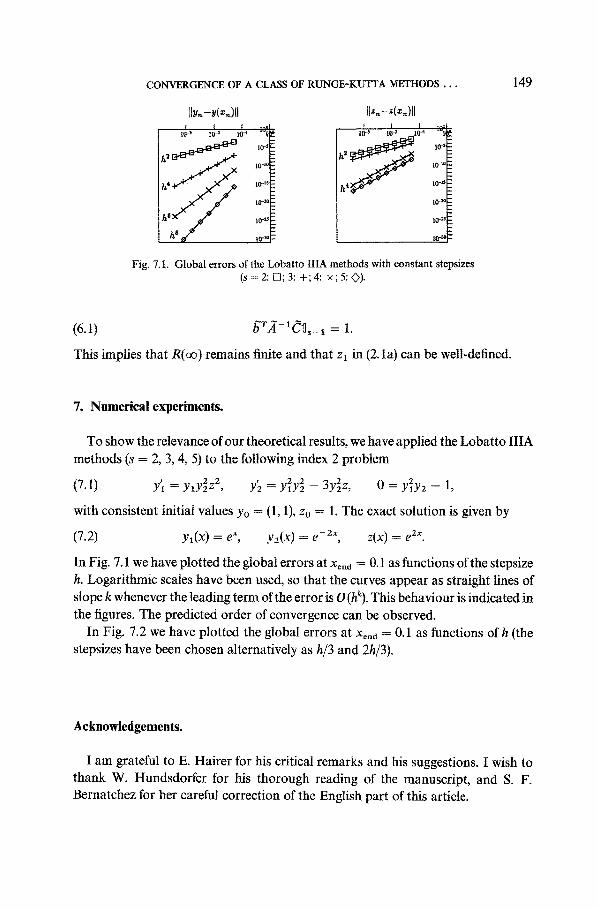
Itu=-y(-,)ll I I I ,~|

10 -~ 10 -2 10 -t "li

h ~ ~ 1°-~ lco0

~hi ~ IO-L~ 16"20

10-~e

10 -3 111 ~ 10 "l "~t~"

111-1 10-15

Fig. 7.1. Global errors of the Lobatto IIIA methods with constant stepsizes (s=2: [];3: +;4: x;5:0).

(6.1) /~TA-1C~s_ 1 = 1.

This implies that R(~) remains finite and that zl in (2. la) can be well-defined.

7. Numerical experiments.

To show the relevance of our theoretical results, we have applied the Lobatto Il iA methods (s = 2, 3, 4, 5) to the following index 2 problem

' 2 2 3yZzz, 0 = y21Y2 1, (7.1) Y'I = Y l Y z z 2 , Y2 = Y l Y 2 - -

with consistent initial values Yo = (1, 1), Zo = 1. The exact solution is given by

(7.2) y l ( x ) = d ' , y z ( x ) = e - zx, z ( x ) = e 2x.

In Fig. 7.1 we have plotted the global errors at Xend = 0.1 as functions of the stepsize h. Logarithmic scales have been used, so that the curves appear as straight lines of slope k whenever the leading term of the error is O (hk). This behaviour is indicated in the figures. The predicted order of convergence can be observed.

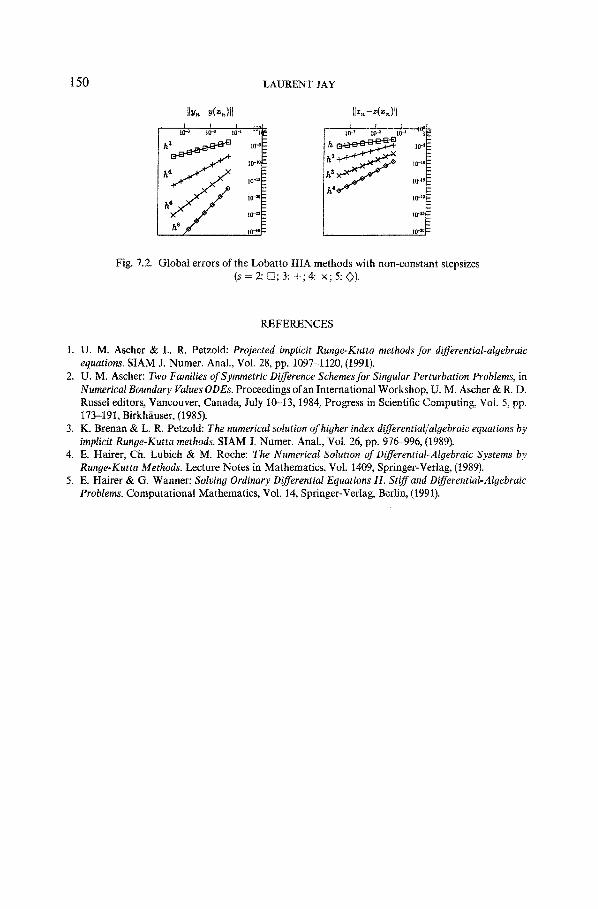
In Fig. 7.2 we have plotted the global errors at Xond = 0.1 as functions of h (the stepsizes have been chosen alternatively as h i 3 and 2h/3).

Acknowledgements.

I am grateful to E. Hairer for his critical remarks and his suggestions. I wish to thank W. Hundsdorfer for his thorough reading of the manuscript, and S. F. Bernatchez for her careful correction of the English part of this article.

150 LAURENT JAY

1 1 t to! 10-~ 10-2 10-1 h i ~ Itr

10-u h 10- t: h ~ / 10-2c

10-~

I0-~ 10-z 113- ~

h ~ lO~

h2 ~ 10 -~°

10-1~ h 4q'° lo -~"

104z

Fig. 7.2. Global errors of the Lobatto IIIA methods with non-constant stepsizes ( s = 2 : D;3: + ;4 : x ;5 : •).

REFERENCES

1. U. M. Ascher & L. R. Petzold: Projected implicit Runge-Kutta methods for differential-algebraic equations. SIAM J. Numer. Anal., Vol. 28, pp. 1097-1120, (1991).

2. U. M. Ascher: Two Families of Symmetric Difference Schemes for Singular Perturbation Problems, in Numerical Boundary Values ODEs. Proceedings of an International Workshop, U. M. Ascher & R. D. Russel editors, Vancouver, Canada, July t0-13, 1984, Progress in Scientific Computing, Vol. 5, pp. 173-191, Birkh~iuser, (1985).

3. K. Brenan & L. R. Petzold: The numerical solution of higher index differential~algebraic equations by implicit Runge-Kutta methods. SIAM J. Numer. Anal., VoL 26, pp. 976-996, (1989).

4. E. Halter, Ch. LuNch & M. Roche: The Numerical Solution of Differential-Algebraic Systems by Runge-Kutta Methods. Lecture Notes in Mathematics, Vol. 1409, Springer-Verlag, (1989).

5. E. Hairer & G. Wanner: Solving Ordinary Differential Equations II. Stiff and Differential-A19ebraic Problems. Computational Mathematics, Vol. 14, Springer-Verlag, Berlin, (1991).