Convection - Dartmouth College

Chapter 7

Convection

SUMMARY: When temperature differences across the system create a gravitation-ally unstable stratification (top-heavy fluid), convection sets in. Two kinds of con-vection are distinguished here: top-bottom convection and penetrative convection.The chapter closes with remarks on the effects of rotation and on methods to sim-ulate convection in computer models.

7.1 Gravitational Instability

Thermal expansion causes warmer fluid to expand thereby decreasing its density.Fluid warmer than its surrounding experiences an upward buoyancy force and tendsto rise, whereas fluid colder than its surrounding tends to sink. Most often, suchdensity differences create a stable stratification, with the lighter fluid floating atopthe denser fluid. The system then allows internal waves (see Section 4.2) or limitedinstabilities (see Sections 5.1 and 5.2). There exist, however, cases when the verticaldensity gradient is inverted, due to cooling at the top of the system or heating atthe bottom. The two primary examples are winter cooling of lakes (heavier fluidcreated near the top) and daytime heating of the lower atmosphere (lighter fluidcreated near the bottom1).

In such case, the fluid still seeks gravitational stability, with the lowest possiblelevel of potential energy, but as long as the destabilizing heat flux persists at oneof the boundaries, such ultimate stage cannot be reached, and vertical motionspersist. Through these ascending and descending motions of light and heavy fluid,respectively, the system conveys heat upward. This is convection.

1Although the sun is above the atmosphere, its radiation occurs mostly in the visible spectrumto which the atmosphere is transparent. The opaque ground absorbs the solar radiation and re-emits it in the form of longer, infrared radiation, which effectively heats the atmosphere frombelow.

121

122 CHAPTER 7. CONVECTION

7.2 Rayleigh–Benard Convection

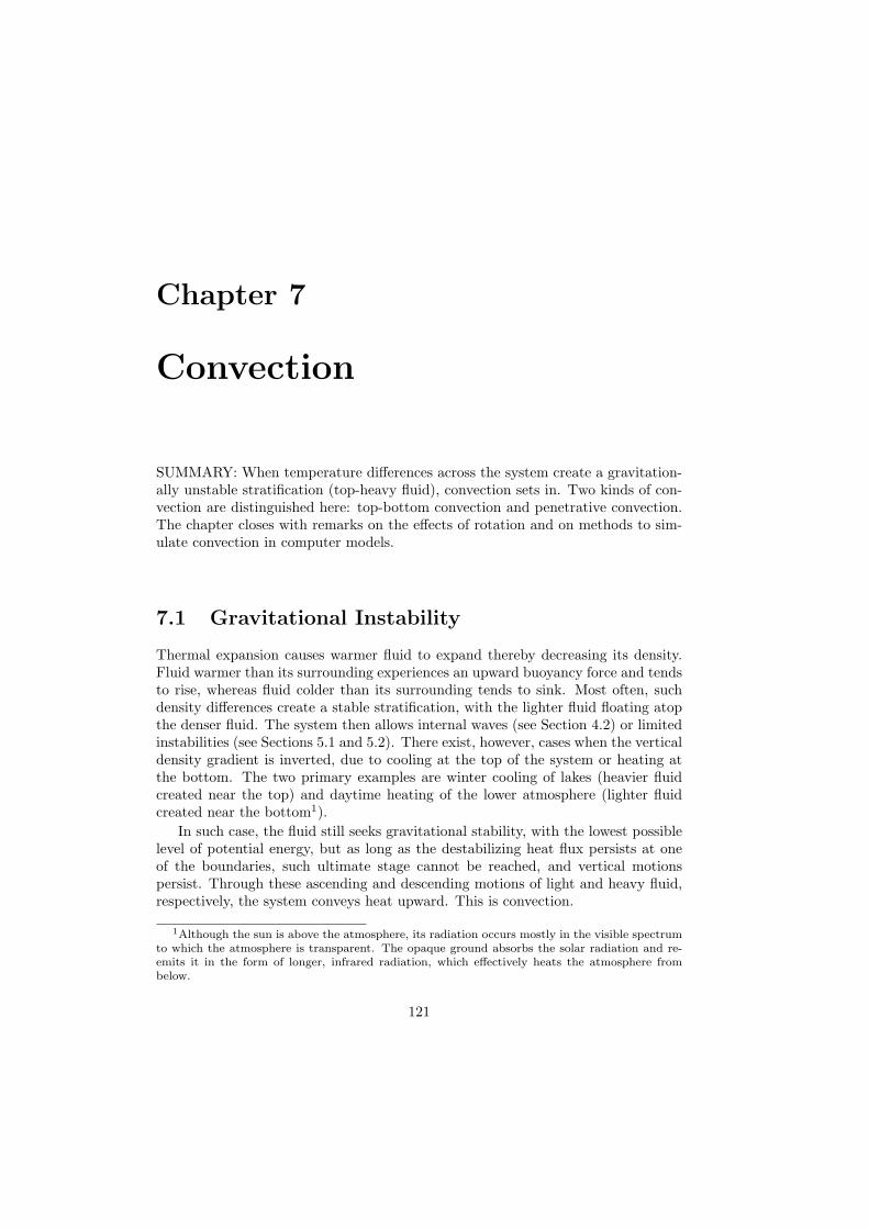
When a thin layer of fluid is heated from below or cooled from above, the upwardheat transfer can be achieved by conduction, that is, in the absence of motion on thepart of the fluid because its viscosity cannot be overcome by the buoyancy forces.However, this can occur only in the rather extreme case of a very thin and veryviscous fluid. Lord Rayleigh2 studied this problem and obtained a straightforwardcriterion. For a horizontal fluid layer of thickness H in contact with a lower tem-perature T along its top surface and with a higher temperature T + ∆T along itsbottom (Figure 7.1), the threshold separating the quiet from the convective regimeis expressed in terms of the Rayleigh number:

Figure 7.1: The convectionproblem studied by LordRayleigh and simulated in thelaboratory by Henri Benard.

Ra =αg∆TH3

νκ, (7.1)

in which α is the thermal expansion coefficient, ν the kinematic viscosity, and κis the thermal diffusivity. Values for water and air at ambient temperatures andpressures are tabulated below.

Table 7.1: Values of physical properties of fresh water (at 10◦C) and air (at 15◦C)at atmospheric pressure.

Physical property Notation Water Air

Thermal expansion coefficient α 2.6× 10−4 /◦C 3.5× 10−3 /◦CKinematic viscosity ν 1.3× 10−6 m2/s 1.5× 10−5 m2/sThermal diffusivity κ 1.4× 10−7 m2/s 2.2× 10−5 m2/s

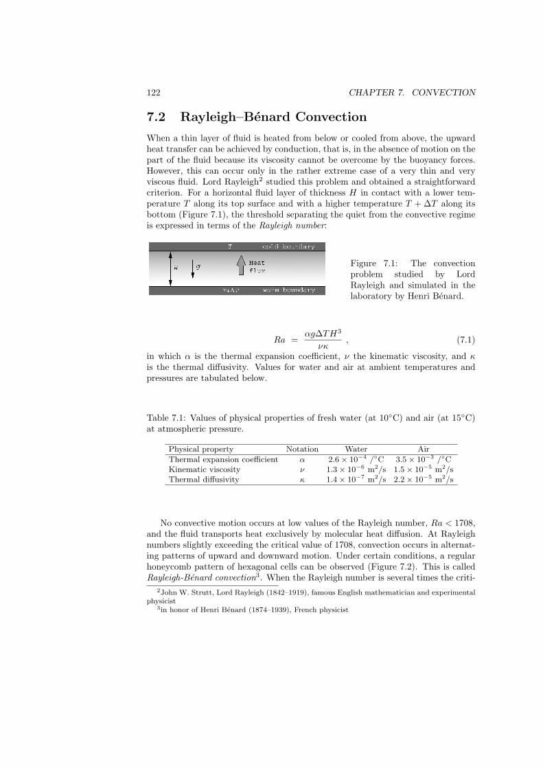
No convective motion occurs at low values of the Rayleigh number, Ra < 1708,and the fluid transports heat exclusively by molecular heat diffusion. At Rayleighnumbers slightly exceeding the critical value of 1708, convection occurs in alternat-ing patterns of upward and downward motion. Under certain conditions, a regularhoneycomb pattern of hexagonal cells can be observed (Figure 7.2). This is calledRayleigh-Benard convection3. When the Rayleigh number is several times the criti-

2John W. Strutt, Lord Rayleigh (1842–1919), famous English mathematician and experimentalphysicist

3in honor of Henri Benard (1874–1939), French physicist

7.3. TURBULENT CONVECTION 123

cal value, these patterns become unstable, oscillatory patterns arise and, for largerRa values, convection becomes chaotic.

Figure 7.2: Time-lapse photo-graph of hexagonal Rayleigh-Benard convective cells. Flowlines are made manifest by alu-minum flakes and 10-second ex-posure. The fluid is rising in thecenter, spreading outward alongthe streaks, and descending atthe edges of the cells. (Photocredit: M. Van Dyke, 1982, AnAlbum of Fluid Motion)

7.3 Top-to-Bottom Turbulent Convection

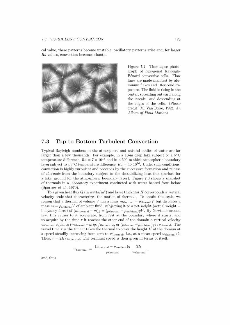
Typical Rayleigh numbers in the atmosphere and natural bodies of water are farlarger than a few thousands. For example, in a 10-m deep lake subject to a 5◦Ctemperature difference, Ra = 7× 1013 and in a 500-m thick atmospheric boundarylayer subject to a 3◦C temperature difference, Ra = 4×1016. Under such conditions,convection is highly turbulent and proceeds by the successive formation and releaseof thermals from the boundary subject to the destabilizing heat flux (surface fora lake, ground for the atmospheric boundary layer). Figure 7.3 shows a snapshotof thermals in a laboratory experiment conducted with water heated from below(Sparrow et al., 1970).

To a given heat fluxQ (in watts/m2) and layer thicknessH corresponds a verticalvelocity scale that characterizes the motion of thermals. To obtain this scale, wereason that a thermal of volume V has a mass mthermal = ρthermalV but displaces amass m = ρambientV of ambient fluid, subjecting it to a net weight (actual weight −buoyancy force) of (mthermal −m)g = (ρthermal − ρambient)gV . By Newton’s secondlaw, this causes to it accelerate, from rest at the boundary where it starts, andto acquire by the time τ it reaches the other end of the domain a vertical velocitywthermal equal to (mthermal−m)gτ/mthermal, or (ρthermal−ρambient)gτ/ρthermal. Thetravel time τ is the time it takes the thermal to cover the height H of the domain ata speed steadily increasing from zero to wthermal, i.e., at a mean speed wthermal/2.Thus, τ = 2H/wthermal. The terminal speed is then given in terms of itself:

wthermal =(ρthermal − ρambient)g

ρthermal

2H

wthermal,

and thus


Figure 7.3: Thermals rising in water above a heated horizontal plate. (From Spar-row et al., 1970)

w2thermal = 2gH

ρthermal − ρambient

ρthermal. (7.2)

Note that the preceding equation could also have been derived by stating conserva-tion of energy: The kinetic energy acquired by the thermal is balanced by an equalreduction in potential energy.

Because the density anomaly is due to a temperature difference, the previousexpression can also be expressed as

w2thermal = 2αgH (Tthermal − Tambient), (7.3)

after using the thermal’s temperature as the reference temperature in the equationof state.

Vertical motion carrying a temperature anomaly is conveying a heat flux, so thata thermal of massmthermal carries a heat anomaly ofmthermalCp (Tthermal−Tambient),in which Cp is the fluid’s heat capacity at constant pressure (1005 J/kg·◦C for airand 4184 J/kg·◦C for freshwater). If n is the number of thermals generated perunit horizontal area and per unit time, then the heat flux Q (heat conveyed perunit area and per unit time) is

Q = mthermal Cp (Tthermal − Tambient) n.

The productmthermaln is the mass carried away by the thermals (per unit horizontalarea and time) and is thus equal to ρthermal f wthermal, in which f is the fractionof the horizontal plane occupied by thermals. Expressed in terms of the thermals’velocity, the heat flux is thus

Q = ρthermal Cp f wthermal (Tthermal − Tambient). (7.4)

7.3. TURBULENT CONVECTION 125

Using (7.3) to eliminate the temperature anomaly Tthermal − Tambient, we obtain:

Q = ρthermal Cp fw3

thermal

2αgH,

which can be solved to obtain the thermals’ velocity in terms of the heat flux:

wthermal =

(2αgHQ

ρthermal Cp f

)1/3

. (7.5)

Dropping the dimensionless factors on the order of unity (2 and f) and replacingthe thermals’ density by the reference density ρ0, we are led to define the followingvertical velocity scale

w∗ =

(αgHQ

ρ0Cp

)1/3

, (7.6)

which by virtue of its construction is representative of (i.e., is a scale for) the verticalmotion of the thermals effecting the convection.

A scale for the temperature fluctuations caused by the thermals can likewise bedetermined. Substituting in (7.4) expression (7.5) for the thermal’s velocity, we cansolve for the thermals’ temperature anomaly:

Tthermal − Tambient =Q

ρthermal Cp f wthermal

=

(Q2

2αgHρ2thermal C2p f2

)1/3

, (7.7)

which suggests the following scale for the temperature fluctuations:

T∗ =

(Q2

αgHρ20 C2p

)1/3

. (7.8)

As thermals carry their heat anomaly across the height H of the system, theycontribute to changing its averaged temperature T according to

dT

dt= ± Q

ρ0 Cp H, (7.9)

as the overall heat budget prescribes. The plus sign is chosen in the case of heatingfrom below, and the minus sign in the case of cooling from above.


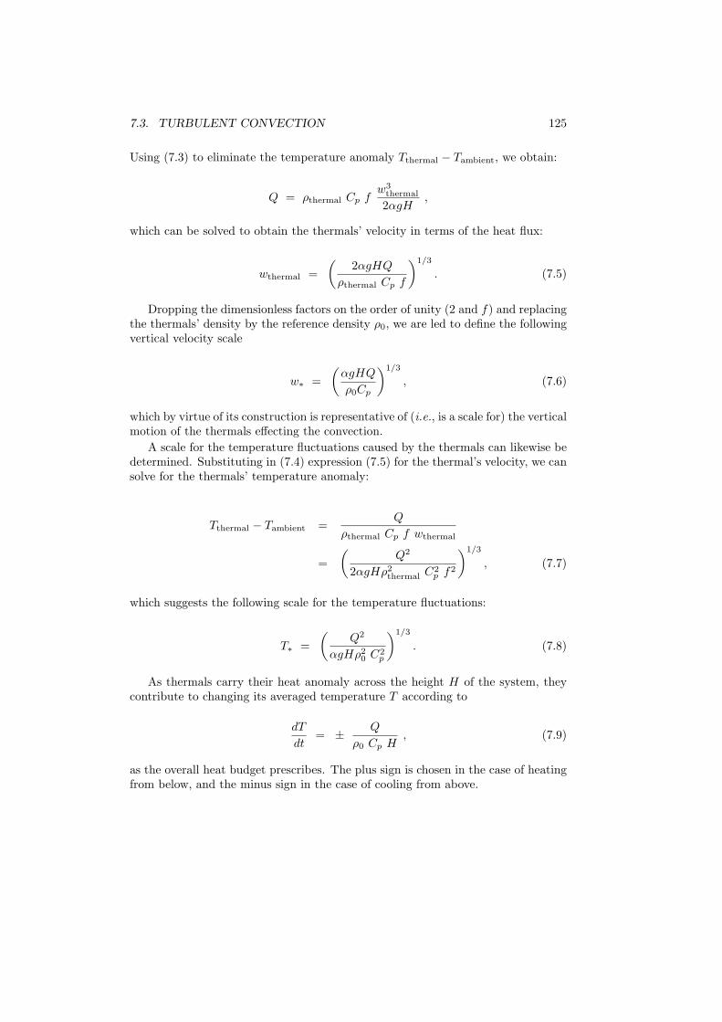
Figure 7.4: Cycle of seasonal heating and cooling in the subarctic Pacific Ocean: (a)Heat flux over the course of the year, and (b) the corresponding thermal structureof the upper ocean. Temperature contours are in degrees Fahrenheit. (From Tullyand Giovando, 1963)

7.4 Penetrative Convection

The previous section considered a fully convecting system, in statistically steadystate, except for the gradual decrease or increase of the overall temperature overtime. In the environment, however, convection often operates against a pre-existingstratification, which it proceeds to erode. For example, a lake is typically strat-ified by summer’s end and when comes autumn, cooling at the surface generatesconvection, which gradually destroys the underlying thermal stratification that hadbeen built over the previous months. As cooling persists, the convective layer growsdeeper and less of the stratification remains, until there is none left and convectionengulfs the entire water column. In the ocean, the same seasonal process occurs,except that the convection is unable to reach the bottom by the time the heatingseason returns (Figure 7.4).

Likewise, the lower atmosphere cools during the night, and by morning theground is covered by a layer of cold air. When the sun rises, the ground absorbs thesolar radiation and heats the atmosphere from below, gradually erasing the night-time stratification. The convective layer, capped by the remnant of stratification iscalled the atmospheric boundary layer (ABL). The photograph in Figure 7.5 reveals

7.4. PENETRATIVE CONVECTION 127

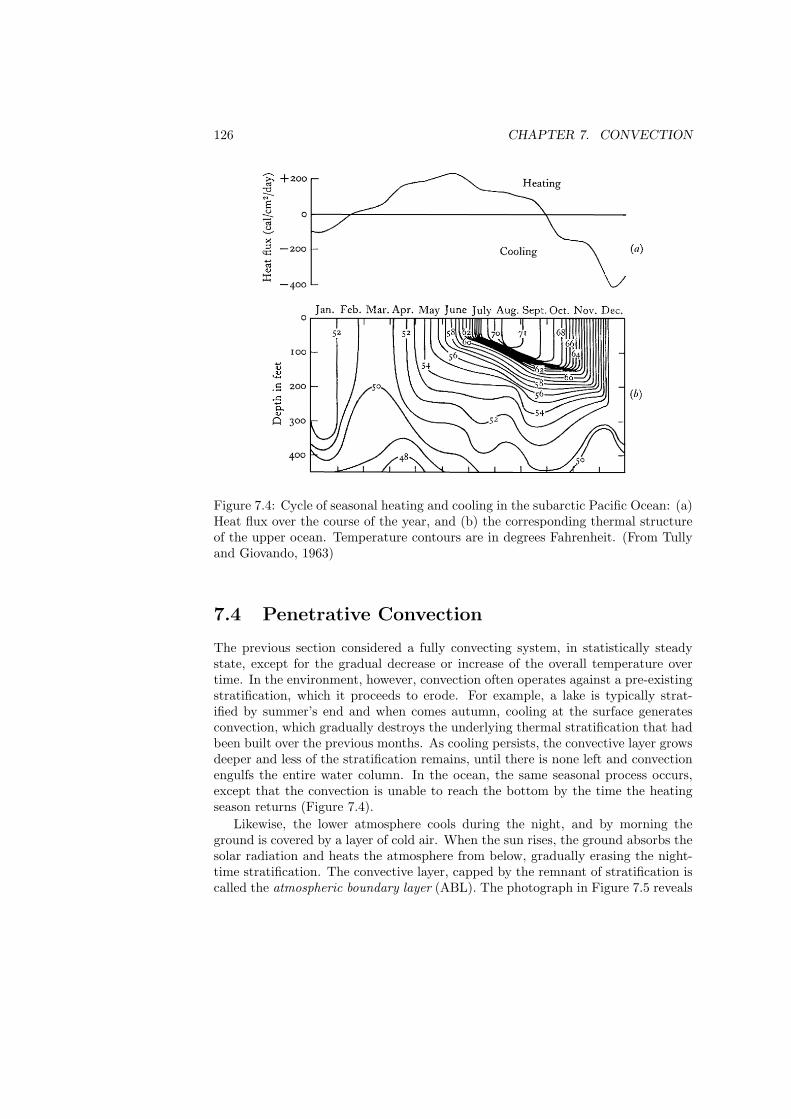
Figure 7.5: Thermals rising upwards and ending in clouds as indicators of atmo-spheric convection. (Photograph by Adrian Thomas)

the presence convection in the lower atmosphere under intense heating, manifestedas wisps of condensation rising from the ground and ending in cloud puffs

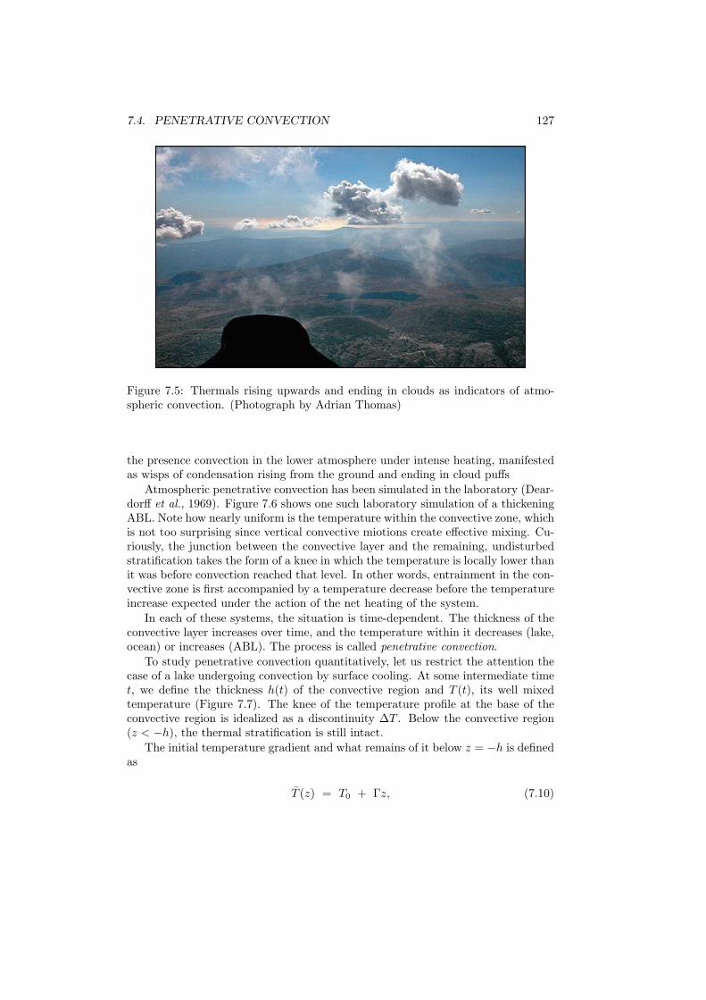
Atmospheric penetrative convection has been simulated in the laboratory (Dear-dorff et al., 1969). Figure 7.6 shows one such laboratory simulation of a thickeningABL. Note how nearly uniform is the temperature within the convective zone, whichis not too surprising since vertical convective miotions create effective mixing. Cu-riously, the junction between the convective layer and the remaining, undisturbedstratification takes the form of a knee in which the temperature is locally lower thanit was before convection reached that level. In other words, entrainment in the con-vective zone is first accompanied by a temperature decrease before the temperatureincrease expected under the action of the net heating of the system.

In each of these systems, the situation is time-dependent. The thickness of theconvective layer increases over time, and the temperature within it decreases (lake,ocean) or increases (ABL). The process is called penetrative convection.

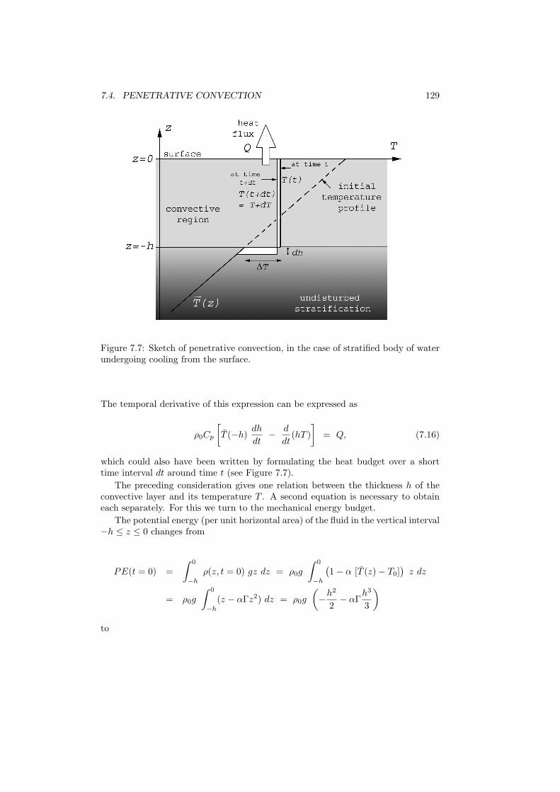
To study penetrative convection quantitatively, let us restrict the attention thecase of a lake undergoing convection by surface cooling. At some intermediate timet, we define the thickness h(t) of the convective region and T (t), its well mixedtemperature (Figure 7.7). The knee of the temperature profile at the base of theconvective region is idealized as a discontinuity ∆T . Below the convective region(z < −h), the thermal stratification is still intact.

The initial temperature gradient and what remains of it below z = −h is definedas

T (z) = T0 + Γz, (7.10)


Figure 7.6: Successive verticalprofiles of temperature in a lab-oratory experiment of penetra-tive convection, wherein a ther-mally stratified layer of wateris heated from below. The la-bels mark the time in minutes.(From Deardorff et al., 1969)

in which T0 is the original surface temperature. The gradient Γ > 0 is takenas constant (linear stratification). To this gradient corresponds the stratificationfrequency N defined from

N2 = αgdT

dz= αgΓ > 0. (7.11)

The temperature at the top of the remaining stratification is then given by

T (−h) = T0 − Γh (7.12)

and the temperature jump at the base of the convective zone is

∆T = T − T (−h)

= T − T0 + Γh. (7.13)

The surface heat flux is denoted as Q (in W/m2) and defined as positive upward(cooling). The overall heat budget (per unit horizontal area) from the time whenthe heat flux began (t = 0) to the present time (t = t) demands:∫ 0

−h

ρ0Cp [T (z) − T (t)] dz =

∫ t

0

Q(t′) dt′, (7.14)

which states that the heat lost in the changing temperature profile between z =−h and the surface is equal to the heat extracted through the surface during theintervening time. Performing the vertical integral, we obtain:

ρ0Cp

[(T0 − T ) h − Γ

h2

2

]=

∫ t

0

Q(t′) dt′. (7.15)


Figure 7.7: Sketch of penetrative convection, in the case of stratified body of waterundergoing cooling from the surface.

The temporal derivative of this expression can be expressed as

ρ0Cp

[T (−h)

dh

dt− d

dt(hT )

]= Q, (7.16)

which could also have been written by formulating the heat budget over a shorttime interval dt around time t (see Figure 7.7).

The preceding consideration gives one relation between the thickness h of theconvective layer and its temperature T . A second equation is necessary to obtaineach separately. For this we turn to the mechanical energy budget.

The potential energy (per unit horizontal area) of the fluid in the vertical interval−h ≤ z ≤ 0 changes from

PE(t = 0) =

∫ 0

−h

ρ(z, t = 0) gz dz = ρ0g

∫ 0

−h

(1− α [T (z)− T0]

)z dz

= ρ0g

∫ 0

−h

(z − αΓz2) dz = ρ0g

(−h2

2− αΓ

h3

3

)to


PE(t) =

∫ 0

−h

ρ(z, t) gz dz = ρ0g

∫ 0

−h

[1− α (T − T0)] z dz

= ρ0g [1− α (T − T0)]

∫ 0

−h

z dz = ρ0g

(−h2

2+ α (T − T0)

h2

2

),

so that the change over time t since convection began is

∆PE = PE(t) − PE(t = 0)

= αρ0gh2

(T − T0

2+

Γh

3

). (7.17)

We further make the drastic assumption — to be duly verified later — thatthe kinetic energy consumed by the sinking thermals is negligible. In other words,we assume that potential energy is barely consumed and merely rearranged. Thisis possible because the raising of the center of gravity by elevating heavier fluidand lowering lighter fluid can be balanced by the dropping of the center of gravityby overall thermal contraction of the fluid under net cooling. Mathematically, wesimply write ∆PE = 0, or

T0 − T

2=

Γh

3. (7.18)

Solving for the instantaneous temperature T in the convective layer, we have

T = T0 − 2Γh

3, (7.19)

which also provides the temperature jump at the base of the convective layer:

∆T =Γh

3. (7.20)

We now have two equations, (7.15) and (7.19), for the two unknowns, the in-stantaneous thickness of the convective layer, h, and its temperature, T . In termsof the cumulated heat flux

∫ t

0Q(t′)dt′, the solution is:

h(t) =

√6

ρ0CpΓ

∫Q(t′)dt′ (7.21)

T (t) = T0 −

√8Γ

3ρ0Cp

∫Q(t′)dt′ , (7.22)

or, in terms of the stratification frequency N defined in (7.11),


h(t) =

√6αg

ρ0CpN2

∫Q(t′)dt′ (7.23)

T (t) = T0 −

√8N2

3αgρ0Cp

∫Q(t′)dt′ . (7.24)

If the heat flux is constant, its integral over time is simply∫Q(t′)dt′ = Qt.

The task is not finished until we have verified that the kinetic energy palesin comparison to the terms in the potential energy. The kinetic energy (per unithorizontal area) is on the order of

KE ∼ 1

2ρ0 h w2

∗,

where w∗ is the thermal’s vertical velocity scale given by (7.6) of the previoussection. Thus,

KE ∼ 1

2ρ0 h

(αghQ

ρ0Cp

)2/3

,

∼ 1

2

(ρ0α

2g2h5Q2

C2p

)1/3

. (7.25)

This is to be compared to one of the terms making the potential energy differencein (7.17), say

∆PE ∼ αρ0gΓh3

3.

The ratio of kinetic to potential energy variations is then found to be

KE

∆PE∼ 3

2

(Q2

αρ20gΓ3C2

ph4

)1/3

∼ 1

(Nt)2/3. (7.26)

The time duration t of the convection (hours in the daily cycle to months in the sea-sonal cycle) is much longer than the stratification time scale 1/N , which is typicallyon the order of seconds and minutes. So, indeed, kinetic energy is minuscule com-pared to the potential energy, and we were justified in neglecting its contributionto the mechanical energy budget. A fortiori, the decay rate of kinetic by frictionalforces is, too, unimportant to the mechanical energy budget.

In a lake, it is not unusual for penetrative convection to reach the bottom by latewinter, thereby resetting the bottom temperature and re-oxygenating the bottomwaters. If cooling persists beyond this time, when no thermal stratification remains,


convection proceeds from top to bottom according to the dynamics exposed in theprevious section.

The previous analysis and equations were derived in the case of a water body be-ing cooled from above. Everything applies to the case of the atmospheric boundarylayer (ABL) being heated from below. One only needs to change the terminologyfrom cooling to heating, downward to upward, etc.

7.5 Convection in a Rotating Fluid

Sinking and rising convective motions create pressure anomalies, which in the pres-ence of the Coriolis force generate circling currents. These tend to confine laterallythe convective motions into coherent vertical plumes, called chimneys. Examplesin the ocean.

Horizontal scale and vertical velocity scale.

7.6 Convection Modeling

Text of section

Problems

7-1. Estimate the Rayleigh number characterizing the convection shown in Figure7.4 during the month of September. (Use freshwater parameter values in theabsence of seawater parameter values.)

7-2. You notice a buzzard soaring in a circling fashion and guess that it is takingadvantage of the upward motion of a thermal. As you happen to have mete-orological gear with you, including a radar profiler (to impress your friends)you determine that the buzzard is flying at an altitude of 60 m and that thetemperature at the center of the bird’s circle is 0.35◦C higher than outside thethermal at the same height. What is the thermal’s vertical velocity? Also,how old is this thermal?

7-3. Based on numbers shown in Figure 7.6, estimate the stratification frequencyN (in 1/s) and heat flux Q (in W/m2) used in the laboratory experimentperformed by Deardorff and collaborators (1969).

7.6. MODELING 133

7-4. The sun has been shining over the sea generating a sustained heat flux of 450W/m2 for three hours, which in turn is generating a growing convective layer.The non-convecting air above this layer is stratified with (potential) temper-ature increasing at the rate of 1.7◦C every 100 m. Estimate the thickness ofthe convective layer after the three hours of sunshine and the increase in airtemperature at sea level over the same time.

7-5. For the preceding problem, compare the velocity of rising thermals w∗ to thegrowth rate dh/dt of the convective layer. Explain physically why it makessense that the former is larger than the latter. [Hint: What would happen ifthe reverse were true?]

7-6. By the end of the summer, Wellington Reservoir (in Western Australia) isthermally stratified with temperature dropping with depth from 26◦C at thesurface to 14◦C at 15 m depth. Below 15 m and all the way down to the bottomat 26 m, the water temperature is uniform at 14◦C. Assuming a constant heatloss of 22 W/m2 to the atmosphere during fall and early winter, how longdoes it take for penetrative convection to erase the summer stratification?Also, trace the vertical velocity w∗ of the sinking thermals during the phaseof penetrative convection and beyond (up to 5 months).

7-7.

7-8.

Documents

Convection - Dartmouth College