rsif.royalsocietypublishing.org

ResearchCite this article: Fuller SB, Karpelson M,

Censi A, Ma KY, Wood RJ. 2014 Controlling free

flight of a robotic fly using an onboard vision

sensor inspired by insect ocelli. J. R. Soc.

Interface 11: 20140281.

http://dx.doi.org/10.1098/rsif.2014.0281

Received: 17 March 2014

Accepted: 20 May 2014

Subject Areas:biomimetics, biomechanics, computational

biology

Keywords:stability, biology-inspired robotics,

velocity feedback, phasic response

Author for correspondence:Sawyer B. Fuller

e-mail: minster@seas.harvard.edu

Electronic supplementary material is available

at http://dx.doi.org/10.1098/rsif.2014.0281 or

via http://rsif.royalsocietypublishing.org.

& 2014 The Author(s) Published by the Royal Society. All rights reserved.

Controlling free flight of a robotic flyusing an onboard vision sensor inspiredby insect ocelli

Sawyer B. Fuller1, Michael Karpelson1, Andrea Censi2, Kevin Y. Ma1

and Robert J. Wood1

1School of Engineering and Applied Sciences and the Wyss Institute for Biologically Inspired Engineering,Harvard University, Cambridge, MA 02138, USA2Laboratory for Information and Decision Systems, Massachusetts Institute of Technology, Cambridge,MA 02138, USA

SF, 0000-0001-6732-6791

Scaling a flying robot down to the size of a fly or bee requires advances in

manufacturing, sensing and control, and will provide insights into mechan-

isms used by their biological counterparts. Controlled flight at this scale has

previously required external cameras to provide the feedback to regulate the

continuous corrective manoeuvres necessary to keep the unstable robot from

tumbling. One stabilization mechanism used by flying insects may be to

sense the horizon or Sun using the ocelli, a set of three light sensors distinct

from the compound eyes. Here, we present an ocelli-inspired visual sensor

and use it to stabilize a fly-sized robot. We propose a feedback controller

that applies torque in proportion to the angular velocity of the source of

light estimated by the ocelli. We demonstrate theoretically and empirically

that this is sufficient to stabilize the robot’s upright orientation. This consti-

tutes the first known use of onboard sensors at this scale. Dipteran flies use

halteres to provide gyroscopic velocity feedback, but it is unknown how

other insects such as honeybees stabilize flight without these sensory

organs. Our results, using a vehicle of similar size and dynamics to the

honeybee, suggest how the ocelli could serve this role.

1. IntroductionFlying robots on the scale of and inspired by flies may provide insights into the

mechanisms used by their biological counterparts. These animals’ flight appara-

tuses have evolved for millions of years to find robust and high-performance

solutions that exceed the capabilities of current robotic vehicles. Dipteran flies,

for example, are superlatively agile, performing millisecond turns during pursuit

[1] or landing inverted on a ceiling [2]. Moreover, these feats are performed using

the resources of a relatively small nervous system, consisting of only 105–107

neurons processing information received from senses carried onboard. It is not

well understood how they do this, from the unsteady aerodynamics of their

wings interacting with the surrounding fluid to the sensorimotor transductions

in their brain [3,4]. An effort to reverse-engineer their flight apparatus using a

robot with similar characteristics could provide insights that would be difficult

to obtain using other methods such as fluid mechanics models or experimentally

probing animal behaviour. The result will be robot systems that will eventually

rival the extraordinary capabilities of insects.

Creating a small flying autonomous vehicle the size of a fly such as that shown

in figure 1 is a difficult undertaking. As vehicle size diminishes, many convention-

al approaches to lift, propulsion, sensing and control become impractical because

of the physics of scaling. For example, propulsion based on rotating motors is inef-

ficient, because heat dissipation per unit mass in the magnetic coils of a rotary

electric motor increases as l22 [5], where l is some characteristic length of the

Figure 1. A 106 mg robot the size of a fly uses a light sensor to stabilize flight,the first demonstration of onboard sensing in a flying robot at this scale. (inset)The visual sensor, a pyramidal structure mounted at the top of the vehicle,measures light using four phototransistors and is inspired by the ocelli of insects(scale bar, 5 mm). (main) Frames taken at 60 ms intervals from a video of astabilized flight in which the only feedback came from the onboard visionsensor. The sensor estimates pitch and roll rates by measuring changes inlight intensity arriving from a light source mounted 1 m above (not shown).This is used in a feedback loop actuating the pair of flapping wings to performcontinuous corrective manoeuvres to stabilize the upright orientation of thevehicle, which would otherwise quickly tumble (see §5). A wire tether transmitscontrol commands and receives sensor feedback, acting as a small disturbancethat does not augment stability. (Online version in colour.)

rsif.royalsocietypublishing.orgJ.R.Soc.Interface

11:20140281

2

vehicle such as wingspan. Combined with increased friction

losses owing to an increased surface-to-volume ratio, exacer-

bated by the need for significant gearing, this results in very

low power densities in small electromagnetic motors [6].

In addition, the lift-to-drag ratio for fixed aerofoils decreases

at small scales because of the greater effect of viscous

forces relative to lift-generating inertial forces at low Reynolds

numbers [7].

The challenges imposed by the small scale of the vehicle

shown in figure 1 extend to sensing and control. The rate of

rotational acceleration increases with decreasing size, scaling

as l21 [8], requiring a feedback sensor with higher bandwidth

[9]. Silicon microfabricated gyroscopes and accelerometers

have recently become small enough to be carried on such

vehicles, primarily because of pressure from the consumer

electronics industry. However, their signal fidelity may be

significantly disrupted by the vibratory environment on

vehicles with flapping wings [10], particularly as the flapping

frequency increases at smaller scales. At a higher level of con-

trol, perceiving attitude and position relative to obstacles or

targets will be essential to achieving autonomy. The global

positioning system used by larger aircraft becomes impracti-

cal at small scale because of insufficient resolution (1–10 m)

and signal disruption in cluttered and indoor environ-

ments [11]. Emissive sensors such as a laser rangefinder are

currently too heavy—the lightest commercially available

scanning rangefinder has a mass of 160 g (Hokuyu URG-

04LX-UG01), three orders of magnitude heavier than the

vehicle in figure 1—and require too much power [11]. Vision

provides a promising solution: cameras can be made small

and low power [12], but, because of the restricted onboard

processing power available, computational requirements

must be minimized. Although the rate of translational accelera-

tion remains constant as scale decreases [8], obstacles may be

nearer, requiring high frame rates and faster processing.

Despite the difficulties imposed by small scale, demonstrations

targeted at such vehicles, to name a few, include navigating

confined spaces [13–15], a high-frame-rate (300 Hz) omnidirec-

tional camera [16], obstacle avoidance using monocular vision

[11,17] or stereo [18], altitude regulation [19,20], hovering [21]

and an initial implementation on a robotic fly [12].

The first fly-sized robot to lift its own weight took inspi-

ration from flying insects [6,22]. For the sake of mechanical

simplicity, this vehicle has two hoverfly-inspired wings

rather than four, driven by piezoelectric actuators performing

a muscle-like reciprocating action [23]. Piezoelectric actuators

were chosen because they scale down more favourably than

electromagnetic motors [5], and the flapping motion generates

unsteady aerodynamics that enhance lift [22]. This prototype is

now being used to better understand and optimize the relevant

fluid mechanics [24,25].

When first flown without guide wires, however, the robotic

fly tumbled [26]. This suggested that, to remain aloft, it requires

constant corrective feedback as is required in unstable fighter

jets [27]. Simulations have suggested that insects have a similar

instability [28–32]. Because of the fast rotational dynamics [8],

control theory dictates that any stabilizing feedback controller

must have a short time delay [9,32]. Controlled flight demon-

strations have so far relied on an array of external cameras to

precisely triangulate the position and orientation of the vehicle

equipped with reflective markers [33], but this approach

cannot extend beyond specific laboratory conditions. Stability

has been achieved with aerofoils such as air dampers [34]

or a tail [18], but this makes the vehicle susceptible to wind

disturbances and sacrifices manoeuvrability.

Here, we address the challenge of achieving stability of a

robotic fly by considering an approach inspired by flying

insects. Most flying insects have three light sensors, distinct

from the compound eyes, that point roughly upwards and

sense light from the sky and/or the Sun [35]. These three sen-

sors, known as the ocelli, are relatively defocused and carry

many neurons that sample the same light information [36,37].

With this optical apparatus, they are much more sensitive to

light than the compound eyes [36], allowing them to quickly

sense changes in the light levels to aid in rapid self-righting

manoeuvres. However, the precise role they play in flight stab-

ility is not well understood [3,38,39]. While dipteran flies are

thought to stabilize flight in part by using mechanosensory

feedback from their elaborate gyroscopic halteres [40,41],

other insect orders have no such apparatus. Hawkmoths use

large vibrating antennae to sense rotations using a similar

mechanism [42,43]. However, the process by which other

species stabilize their flight, such as honeybees, remains

unknown [20]. It is possible that these animals’ flight stabilizer

relies heavily on the ocelli.

From the perspective of autonomous flight control,

an ocelli-inspired light sensor is nearly the simplest possible

visual sensor, minimizing component mass and computational

requirements. A number of previous studies have considered

ocelli-inspired sensors on flying robots, insect-sized [44–47]

or larger [48,49]. In [50], it was shown that an adaptive classifier

could be used to estimate the orientation of the horizon from

omnidirectional camera images. In [44–48,50], the absolute

direction of the light source or horizon relative to the vehicle

was estimated. But whereas aligning to the absolute direction

of a light source or horizon may be a valid approach for

(a) (b)

– 1 mm

Figure 2. The ocelli design consists of four phototransistors soldered to acustom-built circuit board that is folded into a pyramid shape. (a) Theunfolded circuit board before surface-mount components have been added.The transistors’ emitters are connected together (centremost trace) andtied to ground. (b) The larger translucent components are the phototransis-tors and the smaller components are 0201-sized resistors. Lines denote theorientation directions of the sensors. The device weighs 25 mg and isshown beside a US 1 cent coin for scale. (Online version in colour.)

rsif.royalsocietypublishing.orgJ.R.Soc.Interface

11:20140281

3

larger aircraft that fly above obstacles so there is a relatively

clear view to the horizon, smaller vehicles may fly near build-

ings, under foliage or indoors. In these conditions, the horizon

may be obstructed. This causes the direction of light sources to

vary significantly [45]. A control law that aligned the vehicle

with a light source would most likely yield a tilted vehicle

under these conditions, leading to significant lateral acceleration

and dynamic instability.

In this work, we propose an alternative approach in which a

feedback controller applies torque in proportion to angular velocityof the motion of the source of light. This has two benefits. First,

it avoids the need for the light source to be directly above for the

sensor to produce a useful result. Second, we show that an

angular velocity estimate is all that is needed to stabilize the

upright orientation of our flapping-wing robotic fly and

many flying insects. The first was confirmed by previous

work, inspired by observations of derivative-like responses in

insect ocelli [36,37], that showed that ocelli simulated in a vir-

tual environment can estimate angular velocity about the

pitch and roll axes, regardless of initial orientation [49]. The

results also suggested that a linear ocelli response cannot esti-

mate other vehicle motion parameters such as absolute

attitude. A motor controller was described that computed a

time integral of the ocelli angular velocity estimate. Although

this did not require the light to arrive from a known direction,

an estimate computed in this manner would slowly drift

because of accumulated sensor noise. Here, we build on that

work to suggest an alternative approach in which the angular

velocity estimate is instead used directly in a feedback control-

ler. By applying torque in proportion to angular velocity only, it

is possible to harness this vehicle’s flapping-wing dynamics to

achieve a stable upright attitude that does not drift and that

does not require absolute estimate of attitude.

In §2, we describe the design and fabrication of the ocelli-

inspired sensor and flapping-wing robotic vehicle. In §3, we

give a model of the flapping-wing vehicle that shows how its

dynamics can be stabilized by angular velocity feedback, also

known as ‘rate damping’, for both the pitch and roll axes. This

is possible, because, like many flying insects [32,51], the centre

of mass (CM) of the vehicle shown in figure 1 hangs below the

wings [33]. This gives rise to unstable pendulum-like dynamics

that can be stabilized by damping. In §4, we build on previous

analyses of four-sensor ocelli designs to show how to estimate

angular velocity using an arbitrary number of light sensors.

This could allow the number to reduce to three, as in most

flying insects, to save weight. In §5, we demonstrate this feedback

law in operation by stabilizing a fly-sized robot using only feed-

back from the ocelli-inspired light sensor. We conclude with a

discussion about how this work suggests how animals without

gyroscopic feedback, such as the honeybee, could use the fast,

derivative-like reflex mediated by the ocelli [3,36,37,52] to

perform an equivalent role to stabilize their flight dynamics.

2. Sensor and robot fly2.1. Ocelli sensor design and fabricationThe design of the ocelli sensor (figure 2 and shown attached to

the vehicle in figure 1) draws direct inspiration from insects’

ocelli, as in previously described prototypes [48,49,53,54]. Each

sensor is inclined roughly 308 above the horizon (as in flies

[55]) and captures defocused light from an angular field

spanning approximately 1808 that is nearly circularly symmetric.

Our ocelli sensor is custom-fabricated to obtain small mass

(25 mg) and small footprint (4� 4 � 3.3 mm) compatible with

the robotic fly’s payload capacity. The basic structure of

the device is formed by a lightweight folded circuit board.

Traces were fabricated by laser-ablating the copper layer

of copper-clad polyimide. Subsequently, the outline of the

board was cut by laser, and a unidirectional carbon fibre layer

was adhered to the back to increase structural stiffness. Sur-

face-mount components were soldered on by hand, and the

pyramid structure was then hand-folded into shape. Each of

the four light detectors consists of a phototransistor

(KDT00030 from Fairchild semiconductor) in a common-

emitter configuration in series with a 27 kV surface-mount

resistor. The phototransistor has an infrared cut-off filter, redu-

cing its sensitivity to the bright infrared lights emitted by the

motion capture system used to measure flight trajectories. The

voltage reading is taken from the collector of each transistor

and rises with increasing luminance.

2.2. Robotic fly mechanical characteristicsThe flying vehicle used in this work (figure 1) is actuated by a

pair of independently moving wings. By altering signals to

the piezoactuators driving the wings, they can produce suffi-

cient lift to take-off, as well as produce ‘pitch’ and ‘roll’

torques independently. Greater detail about its mechanical

design is given in [33,56].

We define a right-handed coordinate system for the body in

which, with the wings extending laterally along the y-axis and

the body axis hanging downwards in the negative z-direction,

the x-axis (roll) points forward, the y-axis ( pitch) points to the

left and the z-axis (yaw) points upwards (figure 3). Roll torque

is induced by varying the relative stroke amplitudes of the left

versus right wing. Pitch torque is induced by moving the

‘mean stroke angle’—the time-averaged angle of the forward–

backward motion of the wings—in front (þx) or behind (2x)

the CM [56]. Yaw torque can also, in principle, be modulated

[56], but we do not use this capability in this study.

In our current set-up, the robot is given power and con-

trolled through a lightweight compliant tether wire. Power

and control commands are transmitted over four thin and

flexible 51-gauge (0.022 mm diameter) copper wires, each

less than one-quarter the diameter of a human hair. When

present, the ocelli sensor requires six additional wires to

0x

mg

q

tc

fd

fl

rw

u

yz

X

Z

Y

0.3

(a) (b)

1.5wind speed (m s–1)

drag

for

ce (

mN

)

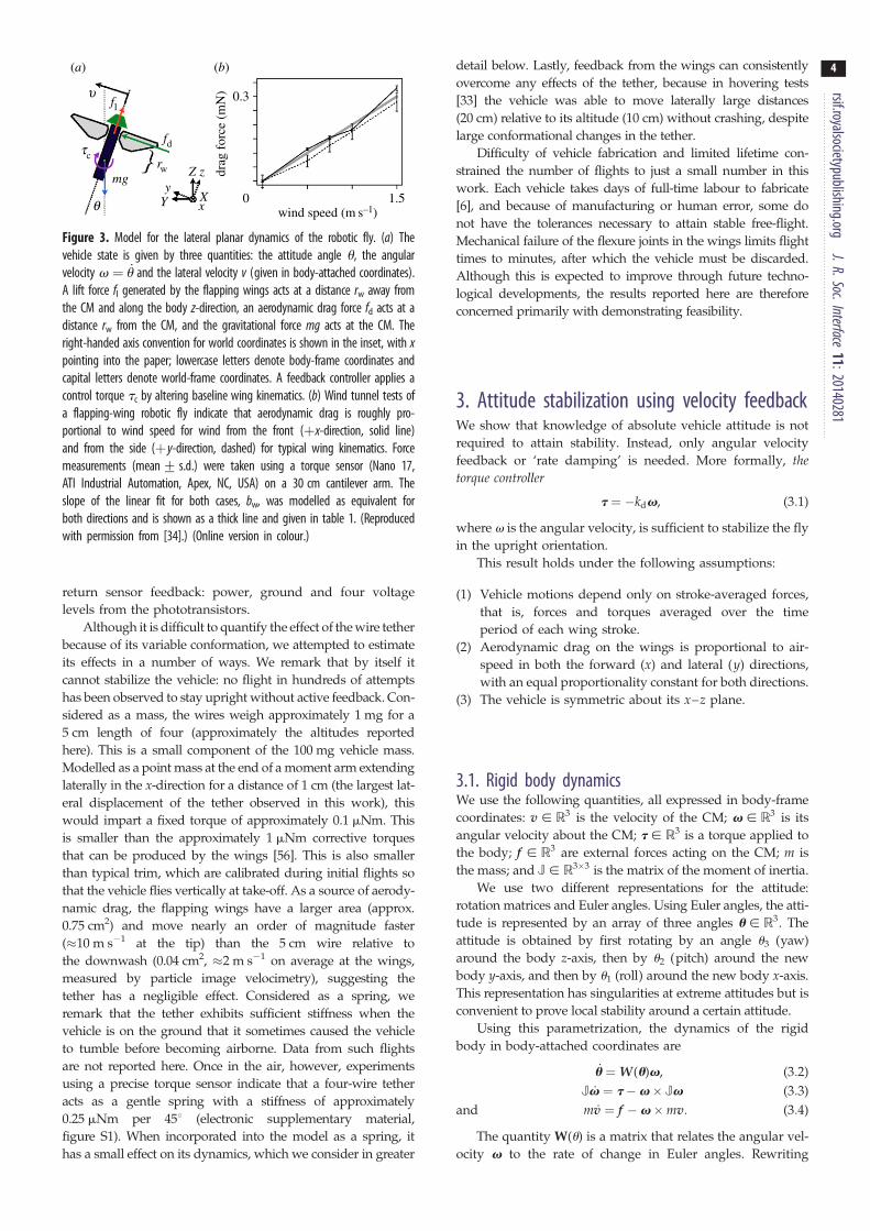
Figure 3. Model for the lateral planar dynamics of the robotic fly. (a) Thevehicle state is given by three quantities: the attitude angle u, the angularvelocity v ¼ _u and the lateral velocity v (given in body-attached coordinates).A lift force fl generated by the flapping wings acts at a distance rw away fromthe CM and along the body z-direction, an aerodynamic drag force fd acts at adistance rw from the CM, and the gravitational force mg acts at the CM. Theright-handed axis convention for world coordinates is shown in the inset, with xpointing into the paper; lowercase letters denote body-frame coordinates andcapital letters denote world-frame coordinates. A feedback controller applies acontrol torque tc by altering baseline wing kinematics. (b) Wind tunnel tests ofa flapping-wing robotic fly indicate that aerodynamic drag is roughly pro-portional to wind speed for wind from the front (þx-direction, solid line)and from the side (þy-direction, dashed) for typical wing kinematics. Forcemeasurements (mean+ s.d.) were taken using a torque sensor (Nano 17,ATI Industrial Automation, Apex, NC, USA) on a 30 cm cantilever arm. Theslope of the linear fit for both cases, bw, was modelled as equivalent forboth directions and is shown as a thick line and given in table 1. (Reproducedwith permission from [34].) (Online version in colour.)

rsif.royalsocietypublishing.orgJ.R.Soc.Interface

11:20140281

4

return sensor feedback: power, ground and four voltage

levels from the phototransistors.

Although it is difficult to quantify the effect of the wire tether

because of its variable conformation, we attempted to estimate

its effects in a number of ways. We remark that by itself it

cannot stabilize the vehicle: no flight in hundreds of attempts

has been observed to stay upright without active feedback. Con-

sidered as a mass, the wires weigh approximately 1 mg for a

5 cm length of four (approximately the altitudes reported

here). This is a small component of the 100 mg vehicle mass.

Modelled as a point mass at the end of a moment arm extending

laterally in the x-direction for a distance of 1 cm (the largest lat-

eral displacement of the tether observed in this work), this

would impart a fixed torque of approximately 0.1 mNm. This

is smaller than the approximately 1 mNm corrective torques

that can be produced by the wings [56]. This is also smaller

than typical trim, which are calibrated during initial flights so

that the vehicle flies vertically at take-off. As a source of aerody-

namic drag, the flapping wings have a larger area (approx.

0.75 cm2) and move nearly an order of magnitude faster

(�10 m s21 at the tip) than the 5 cm wire relative to

the downwash (0.04 cm2, �2 m s21 on average at the wings,

measured by particle image velocimetry), suggesting the

tether has a negligible effect. Considered as a spring, we

remark that the tether exhibits sufficient stiffness when the

vehicle is on the ground that it sometimes caused the vehicle

to tumble before becoming airborne. Data from such flights

are not reported here. Once in the air, however, experiments

using a precise torque sensor indicate that a four-wire tether

acts as a gentle spring with a stiffness of approximately

0.25 mNm per 458 (electronic supplementary material,

figure S1). When incorporated into the model as a spring, it

has a small effect on its dynamics, which we consider in greater

detail below. Lastly, feedback from the wings can consistently

overcome any effects of the tether, because in hovering tests

[33] the vehicle was able to move laterally large distances

(20 cm) relative to its altitude (10 cm) without crashing, despite

large conformational changes in the tether.

Difficulty of vehicle fabrication and limited lifetime con-

strained the number of flights to just a small number in this

work. Each vehicle takes days of full-time labour to fabricate

[6], and because of manufacturing or human error, some do

not have the tolerances necessary to attain stable free-flight.

Mechanical failure of the flexure joints in the wings limits flight

times to minutes, after which the vehicle must be discarded.

Although this is expected to improve through future techno-

logical developments, the results reported here are therefore

concerned primarily with demonstrating feasibility.

3. Attitude stabilization using velocity feedbackWe show that knowledge of absolute vehicle attitude is not

required to attain stability. Instead, only angular velocity

feedback or ‘rate damping’ is needed. More formally, thetorque controller

t ¼ �kdv, (3:1)

where v is the angular velocity, is sufficient to stabilize the fly

in the upright orientation.

This result holds under the following assumptions:

(1) Vehicle motions depend only on stroke-averaged forces,

that is, forces and torques averaged over the time

period of each wing stroke.

(2) Aerodynamic drag on the wings is proportional to air-

speed in both the forward (x) and lateral (y) directions,

with an equal proportionality constant for both directions.

(3) The vehicle is symmetric about its x–z plane.

3.1. Rigid body dynamicsWe use the following quantities, all expressed in body-frame

coordinates: v [ R3 is the velocity of the CM; v [ R3 is its

angular velocity about the CM; t [ R3 is a torque applied to

the body; f [ R3 are external forces acting on the CM; m is

the mass; and J [ R3�3 is the matrix of the moment of inertia.

We use two different representations for the attitude:

rotation matrices and Euler angles. Using Euler angles, the atti-

tude is represented by an array of three angles u [ R3. The

attitude is obtained by first rotating by an angle u3 (yaw)

around the body z-axis, then by u2 (pitch) around the new

body y-axis, and then by u1 (roll) around the new body x-axis.

This representation has singularities at extreme attitudes but is

convenient to prove local stability around a certain attitude.

Using this parametrization, the dynamics of the rigid

body in body-attached coordinates are

_u ¼W(u)v, (3:2)

J _v ¼ t�v� Jv (3:3)

and m _v ¼ f �v�mv: (3:4)

The quantity W(u) is a matrix that relates the angular vel-

ocity v to the rate of change in Euler angles. Rewriting

rsif.royalsocietypublishing.orgJ.R.Soc.

5

equation (3.2) in terms of coordinates gives

_u1_u2_u3

24

35 ¼ 1 sin u1 tan u2 cos u1 tan u2

0 cos u1 � sin u1

0 sin u1 cos u2 cos u1 cos u2

24

35 v1

v2

v3

24

35: (3:5)

We also represent the attitude as a rotation matrix

R(u) [ SO(3). For any vector V [ R3 given in world coordi-

nates, V ¼ Rv, where v [ R3 is the same vector expressed

in body coordinates (figure 3). Using this representation,

equation (3.2) is

_R ¼ Rv�, (3:6)

wherev� [ R3�3 is the skew-symmetric matrix that represents

the cross-product of a vector with v, so that v�v ¼ v� v.

Interface11:20140281

3.2. Analysis of the planar modelAssuming that the z-torque is negligible, we can reduce the

analysis of the six degrees-of-freedom (d.f.) system (equation

(3.4)) to two independent planar systems. We first provide

the planar analysis for the sake of simplicity. The avid

reader can proceed to the subsequent section for the proof

for full rigid body motion.

Consider a state defined by a scalar pitch angle u, a scalar

angular velocity v ¼ _u, and scalar torque t (figure 3). We

show that the controller,

tc ¼ �kdv, (3:7)

that applies a torque proportional to the angular velocity

stabilizes the fly in the upright orientation.

A key element of the model is how the aerodynamic drag

on the wing acts on the rotational dynamics of the robotic fly.

As the rotational dynamics are slow relative to the frequency

of flapping at this scale [20], our analysis considers only

stroke-averaged forces. A test of this vehicle flapping in a

wind tunnel indicated that the stroke-averaged drag force

on the wings is nearly linear with the incident airspeed for

typical wing kinematics (figure 3). This is the case for wind

in both the x- and y-directions. Accordingly, our model for

aerodynamic drag in both cases is

fd ¼ �bwvw,

where vw is the lateral velocity of the point on the airframe at

the midpoint between the two wings. If the vehicle is rotating

at angular velocity v, then the velocity of the wings, when lin-

earized around u ¼ 0, is vw ¼ �rwvþ v, where rw is the

distance from the midpoint of the wings to the CM. Similarly,

the force arising from aerodynamic drag is fd ¼ �bw(v� rwv),

and the torque about the CM owing to this force is

td ¼ �rw fd ¼ bwrwv� bwr2wv. With lift force owing to the flap-

ping wings fl approximately balancing out the weight mg, the

lateral force owing to the inclined gravity vector relative to

the body frame is equal to �mg sin u � �mgu for small u.

A simplified model of the wire tether found using a sensitive

torque sensor suggests it could be incorporated into the

model as a spring with constant ks (electronic supplementary

material, figure S1), according to ts ¼ 2ksu.

Next, we compute the dynamics under the influence of

the torque controller in equation (3.7). In the planar motion

case, we can neglect second-order cross-product terms in

equation (3.4) and equate forces and torques to velocities

according to f ¼ m _v and t ¼ J _v. The linearized equations

of motion about zero pitch angle u can be written as a

state-space dynamical system _q ¼ Aq with the state vector

q ¼ [u, v, v]T expressed in body coordinates, where

A ¼

0 1 0

0 � 1

J(bwr2

w þ kd)1

Jbwrw

�g1

mbwrw � 1

mbw

26664

37775: (3:8)

If desired, the effect of the wire tether can be incorporated

by setting A21 ¼ ks/J, but we neglect its effects in the follow-

ing analysis.

The dynamics are asymptotically stable if the eigenvalues

of A have negative real part. The Routh–Hurwitz criterion

can be used to determine the stability of this system [9].

This allows us to determine the sign of the eigenvalues by

looking at the characteristic equation det(A� lI) ¼ 0, which

gives a polynomial of the form a3l3 þ a2l

2 þ a1l1 þ a0 ¼ 0.

The dynamics are stable if and only if all ak . 0 and a2a1 .

a3a0. If kd . 0, then all of the ak . 0, so the stability

criterion reduces to a quadratic polynomial of the form

b2k2d þ b1kd þ b0 . 0, which has two solution domains. The

negative solution for kd is not stable, because some ak are

negative. The positive solution domain is

kd . kd,

where the bound kd is given by

kd ¼1

2m

� ffiffiffiffiffiffiffiffiffiffiffiffiffiffiffiffiffiffiffiffiffiffiffiffiffiffiffiffiffiffiffiffiffiffiffiffiffiffiffiffiffiffiffiffiffiffiffiffiffiffiffiffiffiffiffiffiffiffiffiffiffiffiffiffiffiffiffiffiffiffiffiffiffiffiffiffiffiffiJ2b2

w þ 2Jb2wmr2

w þ 4Jgm3rw þ b2wm2r4

w

q

� Jbw þmr2wbw

�: (3:9)

Therefore, we have found a lower bound on the gain for the

controller in equation (3.7) that is necessary to achieve

asymptotic stability at [u, v, v] ¼ 0.

The rotational dynamics of the robotic fly given here can be

compared with a pendulum, but are qualitatively different

because of how lateral and rotary motion are coupled. In the

course of flying, if the body is inclined, then the thrust vector

takes on a lateral component, accelerating the vehicle laterally.

As lateral velocity increases, drag from the wings increases.

The lateral drag acts at a location above the CM to exert a

torque that acts to right the vehicle (drag on the body is negli-

gible). In our design, this torque is large enough that it causes

the vehicle to swing with a larger amplitude in the opposite

direction, leading to a growing oscillation that results in tum-

bling. The velocity-dependent action of the controller in

equation (3.7) suppresses this through a damping action [32].

To compute the necessary minimum gain, we estimated

parameters of the robotic fly (table 1). Mass was measured

using a precision scale, and the wing drag factor was

measured in a wind tunnel (figure 3). Moments of inertia

were estimated using a detailed model in computer-aided

design software. The quantity rw was estimated by measur-

ing the distance from the leading edge of the wings to the

approximate point at which the airframe of the robotic fly

balanced on a sharp edge using a ruler under a microscope.

Evaluating equation (3.9) using these parameters gives

kd ¼ 0:9� 10�7 for both xz- and yz-dynamics. Experimental

results (described later) confirm that this value is near the

limiting value between stability and instability, validating

our mathematical results and modelling assumptions.

Table 1. Estimated parameters for the robotic fly shown in figure 1.

quantity symbol quantity units

mass m 81 � 1026 kg

mass of ocelli 25 � 1026 kg

moment of inertia

(x-axis)

J1 1.42 � 1029 kg m2

moment of inertia

( y-axis)

J2 1.34 � 1029 kg m2

moment of inertia

(z-axis)

J3 0.45 � 1029 kg m2

moment of inertia

added by ocelli

(x- and y-axis)

1.8 � 1029 kg m2

wing drag factor bw 2.0 � 1024 Ns m21

distance, CM to wings rw 9 � 1023 m

rsif.royalsocietypublishing.orgJ.R.Soc.Interface

11:20140281

6

3.3. Analysis of the full six degrees-of-freedom rigidbody model

3.3.1. Forces and torquesWe assume that aerodynamic drag, in addition to being pro-

portional to velocity in the x- and y-directions (figure 3 and

[34]), is also proportional to velocity in the z-direction,

although this has not yet been tested. In vector form, the

drag force is thus f d ¼ �bwRTVw, where Vw [ R3 is defined

as the velocity of the point midway between the two wings in

world coordinates. If the body is rotating with angular vel-

ocity v, then the velocity at that point in world coordinates is

Vw ¼ Rv þ (Rv) � (Rrw), where rw ¼ [0, 0, rw]T is the point

where the two wings attach to the airframe and is approximated

as being directly above the CM. Using that (Rv) � (Rrw) ¼

R(v � rw), and that RTR ¼ I, where I is the identity matrix,

we have that

f d ¼ �bwðvþv� rwÞ:

Gravity applies a force directly downwards through the CM and

is given by f g ¼ �mg[� sin u1, sin u2, cos u1 cos u2]T in body

coordinates. The lift force from the wings acts with a magnitude

roughly equal to the force of gravity, fl¼ [0, 0, mg]T and in line

with the CM. Thus, we have that the total external force applied

to the vehicle, expressed in body coordinates, is

f ¼ �bw(vþv� rw)þmgsin u1

� sin u2

1� cos u1 cos u2

24

35:

The torque applied by drag on the wings is

td ¼ �rw � f d ¼ �bw(rw � vþ rw � (v� rw)), and the con-

trol torque is tc ¼ 2kdv (equation (3.1)). Thus, the entire

torque is

t ¼ �kdv� bw(rw � vþ rw � (v� rw)):

3.3.2. Linearized analysis around hoverWe use a linearized analysis to assess stability of the hover con-

figurations (v ¼ 0; v ¼ 0; u1 ¼ 0, u2 ¼ 0, and any value for u3).

We use the local coordinates q ¼ [u1, u2, u3, v1, v2, v3,

v1, v2, v3]T and derive the linearized dynamics _q ¼ Aq valid

around the point q ¼ [0, 0, u3, 0, 0, 0, 0, 0, 0]T.

Consider the rigid body dynamics described by equations

(3.2)–(3.4). Taking the derivative, the second-order cross-

product terms (v� Jv and v�mv) disappear. To fill out

the matrix A, we compute the linearized dynamics and

obtain that

d

dvt ¼ �kdI� bwdiag(r2

w, r2w, 0):

Similarly, we obtain (d/dv)t ¼ �bwr�w, (d/dv)f ¼ bwr�w and

(d/dv)f ¼ �bwI. Because our vehicle is symmetrical, its

moment of inertia is well approximated by

J ¼ diag(J1, J2, J3): Assembling the matrix A, we obtain

A ¼

0 0 0 1 0 0 0 0 00 0 0 0 1 0 0 0 00 0 0 0 0 1 0 0 0

0 0 0�bwr2

w � kd

J10 0 0

bwrw

J10

0 0 0 0�bwr2

w � kd

J20 � bwrw

J20 0

0 0 0 0 0 � kd

J30 0 0

0 g 0 0 � bwrw

m0 � bw

m0 0

�g 0 0bwrw

m0 0 0 � bw

m0

0 0 0 0 0 0 0 0 � bw

m

266666666666666666666666664

377777777777777777777777775

: (3:10)

We can verify that for any kd . kd (equation (3.9)) A has all

eigenvalues with negative real parts, except for a zero eigen-

value corresponding to free state u3, the heading angle of the

vehicle, whose value has no effect on the dynamics. Because it

is sufficient to show that the linearized dynamics are stable to

prove that the full nonlinear system is stable in a neighbourhood

of that equilibrium [9], we have proved that the angular velocity

feedback control law in equation (3.1) stabilizes the robotic fly in

rsif.royalsocietypublishing.orgJ.R.Soc.Interface

11:20140281

7

the upright hovering position, provided that kd . kd, with kd

given by the lower bound in equation (3.9).

An inspection of the rows of A shows that the two planar

systems qx ¼ [u2, v2, v1]T and qy ¼ [u1, v1, v2]T have no

coupling, so that each planar system can be analysed inde-

pendently. This allows for the analysis considered above.

We must emphasize that this only applies for a linearization

around v3 ¼ 0. However, if manufacturing asymmetry gener-

ates a small but constant disturbance torque around the z-axis

(this is commonly the case), then the flapping wings generate

a counter-torque roughly in proportion to the angular vel-

ocity v3 [57], so that v3 does not grow without bound.

Therefore, the fly will stabilize in the upright orientation,

and rotation around the vertical axis will remain small.

A similar analysis suggests that stability could also be

achieved through a mechanical design change that reduces

rw, the distance from the wings to the CM, assuming

the wings themselves provide a small amount of rota-

tional damping. For example, if the wings impart a torque

t ¼ 2cv with c ¼ (1=4)kd, then passive stability is achieved

with 0 , rw , 0.7 mm.

4. Estimating angular velocity using the ocelliHere, we show how to use the ocelli output to produce an esti-

mate v of the angular velocity for use in a feedback controller

(equation (3.1)) to stabilize the robotic fly. We call each photo-

receptor an ‘ocellus’ to highlight the biological inspiration. We

will prove the following result: there exists a matrix L such that theleast-squares estimate of the angular velocity is v t ¼ L _yt, where _yt isthe vector of the time derivatives of each ocellus signal. The result

holds under the following assumptions:

(1) The sensitivity of each ocellus is circularly symmetric.

This is a reasonable approximation for the phototransis-

tors in our sensor prototype and fly ocelli [55].

(2) There is only one static circularly symmetric luminance

source in the environment. This is typically the case

outdoors: the sun is a localized luminance source; a

cloudy sky is a very diffuse luminance source taking on

a hemisphere.

(3) This light source is far away. With this assumption,

translational motion of the vehicle does not induce a sig-

nificant change in the direction of the light source relative

to the vehicle.

(4) There are at least three ocelli, arranged in a non-singular

configuration.

Previous work in the literature has considered the case in which

the ocelli are configured in opposing pairs [45,49]. Here, we give

a geometrical treatment that provides for an arbitrary number of

ocelli in arbitrary directions, permitting either greater feedback

precision or a reduced sensor mass as necessary.

4.1. Ocelli sensor modelLet the sensor be composed by n defocused photoreceptors. The

output of the sensor is an array yt ¼ [y1t , . . . yi

t, . . . , ynt ]

T[ Rn

in which each component is the voltage signal from a single

ocellus, all of which have identical response properties. This vol-

tage is proportional to the luminance in the environment

averaged over the visual sphere in the directions to which the

ocellus is sensitive.

Let m:S2 ! R be the environment ‘map’, so that m(s) is

the luminance in direction s [ S2 on the unit sphere. We

assume this is unchanging according to assumption 3.

Let si [ S2 be the principal direction of the ith ocellus in

body coordinates. If the current sensor attitude is Rt [ SO(3),

then the ocellus is pointing in the direction Rtsi: Using the

assumptions outlined above, it can be shown1 that the

output yit of the ith ocellus at time t is a function only of

the angle between the centre of the light source d,

yit ¼ k(dTRtsi): (4:1)

This assumption has been verified, in practice, for

many lighting conditions when using radially symmetric

and defocused light sensors such as those used in this work

(assumption 2) [45].

4.2. The derivative of the ocellus signal is a linearfunction of angular velocity

Given the sensor model in equation (4.1), we can obtain an

estimate of the angular velocity v. We start by taking the

derivative with respect to time of the sensor output. We

assume the visual scene is static according to assumption 3

so that (d=dt)d ¼ 0. We obtain

_yit ¼ k0(dTRtsi)

d

dtdTRtsi ¼ k0(dTRtsi)dTRtv

�t si:

The last equality comes from the fact that dTRtsi is linear in Rt

so (d=dt)dTRtsi ¼ dT _Rt si [58].

We can linearize around the reference point R ¼ I to obtain

_yit ¼ k0(dTsi)dTv�t si: (4:2)

This expression is a linear function of vt, so we can find

a matrix Mi [ R1�3 such that _yit ¼ Mivt. Using the stan-

dard vector triple product and dot product identities,

we obtain dTv�t si ¼ dTvt � si ¼ vTt (d� si) ¼ (d� si)Tvt and

rewrite equation (4.2) as

_yit ¼ k0(dTsi) (d� si)

Tvt ¼: Mivt: (4:3)

Therefore, we have concluded that the derivative of the ocel-

lus signal is related linearly to the angular velocity.

4.3. Least-squares estimationWe have obtained the expression in equation (4.3) for the

derivative of one ocellus signal. If we write it together for

all ocelli, then we obtain that the derivative of the vector

yt ¼ [y1t . . . yi

t . . . ynt ]T depends linearly on the angular velocity

vt through an n � 3 matrix M,

yt ¼

M1

M2

..

.

Mn

26664

37775vt ¼: Mvt: (4:4)

The least-squares estimate of vt, which assumes equal

noise on all measurements, can be written as

v t ¼ (MTM)�1MT yt ¼:

L yt : (4:5)

This estimate has a number of restrictions. First, the com-

ponent of vt parallel to d cannot be estimated because it is in

the null space of M. This is because each row of M is the result

of a cross-product with d (scaled by k0), so each is orthogonal

rsif.royalsocietypublishing.orgJ.R.Soc.Interfac

8

to d. Together, these rows constitute a plane that is the kernel of

this matrix, and the pseudo-inverse provides only the projection

ofvt onto this plane. This subspace is further restricted to a line if

d and all si are coplanar, because, in that case, all rows of M are

linear multiples of each other. Second, the row Mi is zero when-

ever d ¼+si, because, at these points, d� si is zero. It is also zero

when k0 is zero for any ocellus, such as when the light source is

entirely outside of its field of view, so that angle changes have no

effect on its response. Third, the magnitude of the estimate v t

varies linearly with k0 and thus with the brightness of the light

source function k.

This formulation allows for an arbitrary arrangement of

an arbitrary number of ocelli. As few as two can estimate

the two essential components of vt to provide stability

if the luminance function k is known. If it is not, then

redundant sensors can be used to estimate k [47].

e11:20140281

4.4. Specifics of the four-ocellus designIn our design, the directions of the four ocelli are

closely approximated by s1, s3 ¼ +ffiffiffi3p

=2, 0, 1=2� �T

and

s2, s4 ¼ 0, +ffiffiffi3p

=2, 1=2� �T

. This arrangement has the follow-

ing characteristics:

(1) The ocelli are arranged in pairs that are redundant, so

that the overall illumination level k could be estimated

and divided out, as in [47].

(2) They are tilted in a slight upwards direction, so that a

light source above the vehicle will be detected by all of

them in the course of normal manoeuvring so that

k(dTRsi) = 0. A tilt angle of approximately the same

value, 408, was found to be optimal for estimating

angular rate in [49].

(3) None is tilted so far upwards that it will be pointed

directly at the light source in the course of normal

manoeuvring so that d� si= 0.

(4) The pairs are arranged orthogonally to provide orthog-

onal components of v, simplifying control design [44,45].

In the case of the light source directly overhead

(d ¼ [0, 0, 1]T), the M matrix (4.4) is given by

M ¼

0kffiffiffi3p

20

� kffiffiffi3p

20 0

0 � kffiffiffi3p

20

kffiffiffi3p

20 0

2666666666664

3777777777775

:

In this case, the quantity v3 (the z-component of v) is

not observable, because d is directly above, but for hovering it

is sufficient to leave it uncontrolled, so long as it remains small.

For the other two components, the matrix pseudo-inverse has

the form

v1

v2

� �¼ L _y ¼

ffiffiffi3p

k0 �

ffiffiffi3p

k0

0 �ffiffiffi3p

k0

ffiffiffi3p

k

2664

3775 _y, (4:6)

where k ¼ k0(dTRsi)jR¼I ¼ k0(dTsi) is a constant. A new output

defined by subtracting opposing pairs of ocelli according

to y ¼ [ya, yb] ¼ [y1 � y3, y4 � y2]T [45] recovers a simplified

relation similar to that given elsewhere for a pair of ocelli [49],

v t ¼2ffiffiffi3p

k_yt: (4:7)

If the light is not directly overhead, but at some unknown

angle, then the quantity k may be different for that orientation.

However, by combining equations (4.7) and (3.1), it can be

seen that as long as it can be ensured, by making kd sufficiently

large, that kd=k . kd=k0, where k ¼ k0 when the light source is

directly overhead, then the control law given by (3.1) is asymp-

totically stable.

5. Flight tests5.1. Flight arenaWe performed flights tests in a motion capture arena with an

array of calibrated cameras (T040-series; Vicon, Oxford, UK).

Each camera emits bright infrared that is reflected from

a number of retroreflective markers mounted on the vehicle,

so that its position and orientation can be reconstructed in

real-time for later analysis. Rotation about yaw (z) was left uncon-

trolled in these experiments. In all flights, computations to

generate signals for the piezoelectric actuators to drive wing

motion, as well as to map desired control torques to these signals,

were performed on an XPC Target, a desktop computer running

a real-time operating system (MathWorks, Natick, MA, USA).

Analogue voltage outputs from this computer were amplified

by high-voltage amplifiers and transmitted to the robotic fly

through the wire tether. The compliant wire tether has a small

effect on vehicle dynamics, as detailed in §2.2.

In flights controlled by feedback from motion capture, pos-

ition and orientation estimates were sent by serial cable to the

control computer. In these tests, the estimate v was calculated

by smoothing the motion capture estimates u with a third-

order Butterworth filter with a 40 Hz cut-off frequency, taking

the derivative, and multiplying by the matrix W (equation (3.5)).

For flights in which feedback from the ocelli was used,

illumination was provided by a 150 W halogen bulb at 66%

brightness mounted 1.5 m above the vehicle (Dolan-Jenner

MI-150 fibre-optic illuminator; Edmund Optics, Barrington,

NJ, USA). The control computer measured voltages from the

four phototransistors using an analogue-to-digital data acqui-

sition board (National Instruments). The infrared flashes from

the motion capture cameras, at 500 Hz with a one-eighth duty

cycle, were so bright that they saturated the phototransistors,

regardless of orientation because of reflections from the

ground surface. Accordingly, they did not provide any orien-

tation information. After this initial transient, the voltage

decayed to an attitude-dependent steady-state value (figure 4).

A digital filter recovered these steady-state values by filtering

with a third-order Butterworth filter with a 20 Hz cut-off fre-

quency to smooth out the sudden flashes, as well as the 60 Hz

AC ripple from the light source (figure 4). To calculate the esti-

mate of k in equation (4.7), we rotated the robot by 458 in either

direction and measured the resulting quantity y4 2 y2 to

compute the slope.

5.2. ResultsExperiments provide empirical evidence that the control law

given by equation (3.1) gives stability. In flights without the

ocelli attached in which the estimate v was provided by

04.30 4.35 4.40

time (s)4.45 4.50

2

ocel

li ou

tput

(V

)

4

6(a)

(b) (c)

(d)

0–100 –50 0 50

–5

0

–5

1000

–60–100

100

0

–40 –20angle (measured by motion capture, deg)

angl

e (e

stim

ated

by

ocel

li, d

eg)

0 20 40 60

angle (°) angle (°)

2

ocel

li ou

tput

(V

)

4

6

Figure 4. Calibration of the ocelli-inspired visual sensor. (a) Voltage readings y2 (black) and y4 (grey) from an opposing pair of phototransistors, before filtering (theeffects of the one-eighth duty cycle, 500 Hz infrared flashes of the motion capture cameras can be seen as spikes followed by a short transient decay) and after(smooth trace showing trend), taken during a calibration in which the robotic fly was held by tweezers as it was rotated by hand in the motion capture arena. (b) Tomeasure the approximate acceptance profile ~k of the phototransistor, it was rotated under the fibre-optic light source, approximately a point source. The responsespans a range of approximately 1608 (black) and resembles a Gaussian function with s ¼ 618 (thick grey line, fit performed by fminsearch). (c) y2 (black),y4 (grey) and yb ¼ y4 2 y2 (dashed), plotted against measurements from the motion capture system. The slope of this line at zero angle corresponds to k inequation (4.7). A third-order polynomial fit of angle u2 to yb using the Matlab command polyfit is shown (thick grey line). (d ) This polynomial was used toestimate u2 from the ocelli responses at u1 ¼ 0 (red) compared with the estimate from motion capture (black) and shows a close correspondence for the range of+608. If the ocelli are inclined about the other axis at u1� 308, the estimate is not significantly perturbed (dashed grey line). (Online version in colour.)

rsif.royalsocietypublishing.orgJ.R.Soc.Interface

11:20140281

9

motion capture using a gain of kd ¼ 2 � 1027, well into the

region of stability, the robotic fly remained upright during the

course of the flight before drifting out of the tracking volume

of the motion capture arena. In these flights, only the rate damp-

ing feedback law was being tested: neither altitude nor lateral

position was under feedback control so small asymmetries in

flapping kinematics generated non-zero lateral thrust.

To further test the validity of the model given by equation

(3.8), we observed the natural dynamics of the robotic fly in

flight with a gain of kd ¼ 1.0 � 1027, just at the threshold of

stability. In this flight, it exhibited sinusoidal oscillations simi-

lar to those of a simulation of the model in equation (3.8)

(figure 5). When tested with gains of 0.75 � 1027 or lower,

the vehicle did not remain upright. This shows that the

model and parameters given in table 1 are close to their true

values and that un-modelled effects do not have a large

impact on vehicle dynamics.

A demonstration that the robotic fly can be stabilized exclu-

sively using feedback from the ocelli is shown in figure 6 and in

the electronic supplementary material, video S2. In this exper-

iment, the ocelli sensor was attached to the vehicle and

provided the estimate v . The added mass and inertia of the

ocelli increased the minimum gain to kd ¼ 1:6� 10�7. Using

a gain of kd ¼ 2 � 1027 as above, the fly successfully remained

upright during a 0.3 s climbing phase (approx. 40 wingstrokes)

before the wiring reached its limit. The vehicle remained

upright, but performed rotational oscillations about pitch

and roll, the result of aggressive corrective manoeuvres. With-

out this feedback, the vehicle quickly tumbled (figure 6, inset).

The oscillating instability in the ocelli-stabilized flight was

likely to be due to the nonlinearity of torques exceeding the

pre-programmed actuator limit, owing to an overestimate of

v near the upright orientation. In addition, if at take-off the

vehicle was inclined at juj .308, then this fell outside the

range in which the estimate of v was valid, causing tumbling.

The maximum inclination during this flight was approximately

108, suggesting that torques owing to the torsional stiffness of

the wire tether (§3.2; approx. 0.16 mNm) should have a small

effect relative to control torques.

To mitigate the effect of variable gain and consequent

actuator saturation, and to extend the range of permissible

inclination angles, we performed third-order least-squares fit

of u2 measured by motion capture to yb across a range of

+608 using the Matlab command polyfit, using this fit for

both axes. During flight, evaluating this polynomial requires

minimal additional computation. With this calibration, the

0.1 0.2 0.3 0.4 0.5 0.6 0.7 0.8

−20

−15

−10

−5

0

5

10

15

20

25

time (s)

Eul

er a

ngle

q (

°)

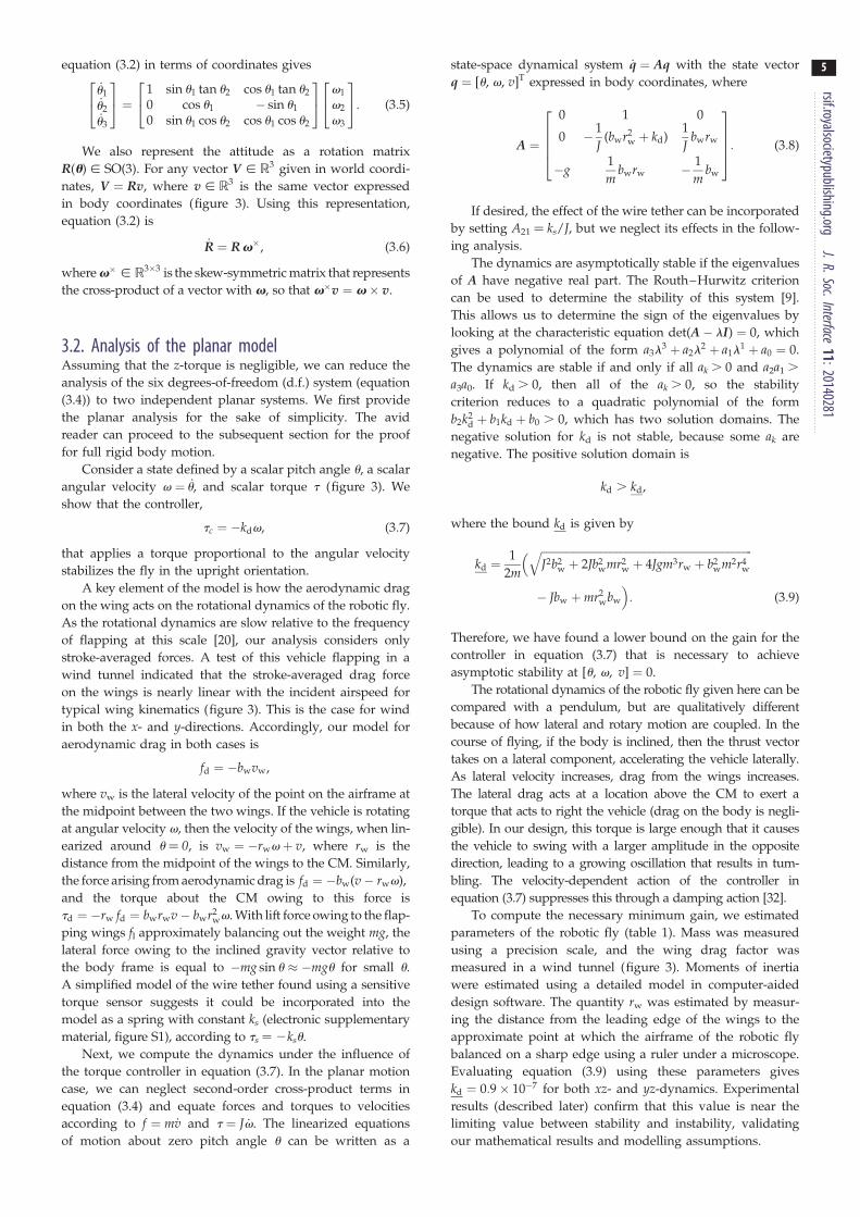
Figure 5. An empirical test of the robotic fly in flight with angular velocityfeedback alone from motion capture, with a gain of kd ¼ 1.0 � 1027 ( justat the threshold of stability), shows that it undergoes rotational oscillations.The unfiltered Euler angles u1 and u2 measured by motion capture (rotationabout body x-axis and y-axis, respectively) are shown in black and grey. Alinear simulation of the robotic fly dynamics (equation (3.8)) with thesame gain, an initial lateral velocity of 0.3 m s21 (thick black line), and par-ameters from table 1 shows similar behaviour, providing empirical support ofthe model proposed in equation (3.8). If the wire tether is incorporated intothe model as a torsional spring (§3.2), then it has a small effect on dynamics(dashed line). Other differences may be due to effects not accounted for inthe model such as un-modelled aerodynamic forces.

rsif.royalsocietypublishing.orgJ.R.Soc.Interface

11:20140281

10

region of operation expanded from roughly +308 to +608(figure 4). A motion capture estimate is not necessary, in prin-

ciple, to perform this calibration; it could easily be performed

using a potentiometer, as in [47]. In flights with this calibration,

the orientation was more stable and the estimate v matched

the motion capture estimate more closely (figures 1 and 7).

Although this calibration improved performance for only a

specific lighting condition, it is possible this could be extended

to improve performance in more general conditions. This could

be achieved by performing a least-squares fit using data taken

from a range of expected lighting scenarios. Our model of the

wire tether indicates it could have imparted torques as high

as 0.24 mNm when the vehicle reached an 188 inclination,

about half the magnitude of the control torques in this trial.

To further demonstrate the utility of the proposed control

law, we performed an additional flight in which this cali-

brated ocelli feedback was combined with the aerodynamic

‘ground effect’ to maintain altitude. The ‘ground effect’ is

an increase in aerodynamic lift that occurs in close proximity

to a horizontal surface [14]. In this flight, both upright orien-

tation and altitude were maintained for a prolonged period of

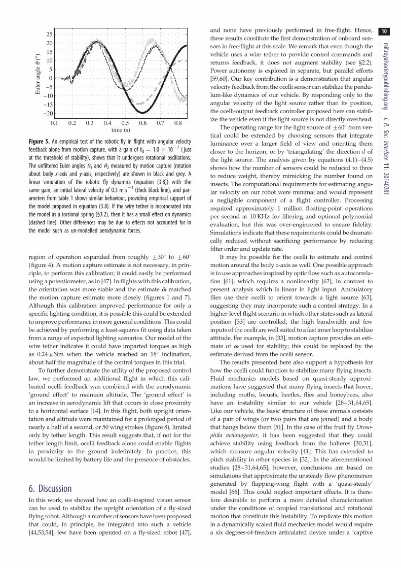
nearly a half of a second, or 50 wing strokes (figure 8), limited

only by tether length. This result suggests that, if not for the

tether length limit, ocelli feedback alone could enable flights

in proximity to the ground indefinitely. In practice, this

would be limited by battery life and the presence of obstacles.

6. DiscussionIn this work, we showed how an ocelli-inspired vision sensor

can be used to stabilize the upright orientation of a fly-sized

flying robot. Although a number of sensors have been proposed

that could, in principle, be integrated into such a vehicle

[44,53,54], few have been operated on a fly-sized robot [47],

and none have previously performed in free-flight. Hence,

these results constitute the first demonstration of onboard sen-

sors in free-flight at this scale. We remark that even though the

vehicle uses a wire tether to provide control commands and

returns feedback, it does not augment stability (see §2.2).

Power autonomy is explored in separate, but parallel efforts

[59,60]. Our key contribution is a demonstration that angular

velocity feedback from the ocelli sensor can stabilize the pendu-

lum-like dynamics of our vehicle. By responding only to the

angular velocity of the light source rather than its position,

the ocelli-output feedback controller proposed here can stabil-

ize the vehicle even if the light source is not directly overhead.

The operating range for the light source of +608 from ver-

tical could be extended by choosing sensors that integrate

luminance over a larger field of view and orienting them

closer to the horizon, or by ‘triangulating’ the direction d of

the light source. The analysis given by equations (4.1)–(4.5)

shows how the number of sensors could be reduced to three

to reduce weight, thereby mimicking the number found on

insects. The computational requirements for estimating angu-

lar velocity on our robot were minimal and would represent

a negligible component of a flight controller. Processing

required approximately 1 million floating-point operations

per second at 10 KHz for filtering and optional polynomial

evaluation, but this was over-engineered to ensure fidelity.

Simulations indicate that these requirements could be dramati-

cally reduced without sacrificing performance by reducing

filter order and update rate.

It may be possible for the ocelli to estimate and control

motion around the body z-axis as well. One possible approach

is to use approaches inspired by optic flow such as autocorrela-

tion [61], which requires a nonlinearity [62], in contrast to

present analysis which is linear in light input. Ambulatory

flies use their ocelli to orient towards a light source [63],

suggesting they may incorporate such a control strategy. In a

higher-level flight scenario in which other states such as lateral

position [33] are controlled, the high bandwidth and few

inputs of the ocelli are well suited to a fast inner loop to stabilize

attitude. For example, in [33], motion capture provides an esti-

mate of v used for stability; this could be replaced by the

estimate derived from the ocelli sensor.

The results presented here also support a hypothesis for

how the ocelli could function to stabilize many flying insects.

Fluid mechanics models based on quasi-steady approxi-

mations have suggested that many flying insects that hover,

including moths, locusts, beetles, flies and honeybees, also

have an instability similar to our vehicle [28–31,64,65].

Like our vehicle, the basic structure of these animals consists

of a pair of wings (or two pairs that are joined) and a body

that hangs below them [51]. In the case of the fruit fly Droso-phila melanogaster, it has been suggested that they could

achieve stability using feedback from the halteres [30,31],

which measure angular velocity [41]. This has extended to

pitch stability in other species in [32]. In the aforementioned

studies [28–31,64,65], however, conclusions are based on

simulations that approximate the unsteady flow phenomenon

generated by flapping-wing flight with a ‘quasi-steady’

model [66]. This could neglect important effects. It is there-

fore desirable to perform a more detailed characterization

under the conditions of coupled translational and rotational

motion that constitute this instability. To replicate this motion

in a dynamically scaled fluid mechanics model would require

a six degrees-of-freedom articulated device under a ‘captive

0.4

–1

–10

0

10

–0.05

0

0.05

0

1

0.6time (s)

cont

rol t

orqu

e(N

m×

10–6

)w

(ra

d s–1

)po

sitio

n (m

)

y (m)

z (m)

0

0.040

0.06

0.040

x (m)

(a)

(b)

(c)

(e)

(d)

Figure 6. Take-off in which the ocelli were using a purely linear feedback law. (a) The camera was aligned with the positive y-axis and the time interval betweenframes is 66 ms. Without feedback, the vehicle quickly tumbles (inset) (also see electronic supplementary material, video S2). (b) Coordinates of flight trajectoryestimated by motion capture: z (solid), x (dashed) and y (dash-dotted). (c) The angular velocity v measured by motion capture (solid lines) versus estimate fromocelli (dashed); v 2 is black and v 2 is grey. Ripple owing to the flapping wings can be observed in the pitch rate estimate. At small u1, the estimate of roll divergesfrom the true value. (d) Pitch and roll torque commands from the controller (solid) are inversely proportional to angular velocity; a safety saturation block limitedthe control command to the wings. (e) Trajectory measured by the motion capture system rendered at every 20 ms. The vertical line is equal to the length of thevehicle and denotes the direction of its long axis. Grey lines in the background show projections of the trajectory onto the xy, xz and yz planes, and the blue line is aprojection of the vehicle x-axis onto the xy plane to show the vehicle’s heading. (Online version in colour.)

0.4

–1

–10

0

10

–0.05

0

0.05

0

1

0.6time (s)

cont

rol t

orqu

e(N

m×

10–6

)w

(ra

d s–1

)po

sitio

n (m

)

y (m)

z (m)

0

–0.04

0

0.04

0.040

x (m)

(a)

(d)(b)

(c)

Figure 7. Data from take-off flight shown in figure 1. In this flight, the ocelli werecalibrated to have a larger operating regime. The lower gain avoids actuator satur-ation and rotatory oscillation. As in figure 1, (a) shows vehicle position, (b) shows acomparison of angular velocity estimates, (c) shows control torque commands, and(d) is a three-dimensional plot of the vehicle trajectory. (Online version in colour.)

rsif.royalsocietypublishing.orgJ.R.Soc.Interface

11:20140281

11

trajectory’ to simulate its inertia in a large tow tank [57]. This

has not yet been achieved. Using a computer instead to

perform computational fluid dynamics simulations would

require a large fluid volume that could require a prohibitive

amount of computation power [67–69]. Another approach is

to carefully manipulate sensory feedback available to alert,

behaving animals [70,71]. However, precisely controlling

sensory input during flight is difficult because of the small

size of the animal. In addition, multiple modes of sensory feed-

back are typically required to stay aloft [3], making it difficult

to isolate the effects of a single sensory organ. Hence, our

robotic fly constitutes a new method to probe insect fluid mech-

anics that avoids these difficulties.

Our results, particularly those in figure 5, support the

view proposed in [30–32] and others that angular velocity

feedback or ‘rate damping’ is sufficient for upright stability

in Drosophila and similarly shaped species. While the robotic

fly and these vehicles are not identical, the approximations

made in the model given in §3 apply equally to both the

robot and these animals. One difference, however, is that in

these animals the body hangs diagonally [32,51] rather verti-

cally as in our vehicle. In both cases, however, the CM is

centred below the wings. For these animals, the inertia

matrix has off-diagonal xz terms that couple torques in the

x-direction to motions about the z-axis and vice versa, but

it can be shown that this does not alter the stability of the

system. To provide a particular example, we consider the

honeybee. In table 2, we give the equivalent parameters for

the honeybee Apis mellifera, which has similar size and

weight to our vehicle. These were derived from measure-

ments and calculations in [32,51]. Drag on the wings is

higher probably because of the higher typical flapping

frequency of bees (197 Hz) compared with our vehicle

(120 Hz), but the moment arm rw is much shorter. In the

case of the honeybee, the model suggests that the minimum

necessary damping gain to achieve upright stability is similar

to that of our robotic fly (table 2).

In insects, studies have suggested that the ocelli mediate

a fast, derivative-like reflex that acts in corrective flight

manoeuvres. Neural recordings of the large L-neurons in the

−0.10−0.05

0

−0.10

−0.05

0

00.010.02

x (m)y (m)

z(m

)

Figure 8. Altitude control and upright stability using only onboard feedback.The ocelli provided feedback to maintain upright while the aerodynamic‘ground effect’ maintained altitude. During the first 0.3 s of flight duringtake-off, the lift was slightly larger, after which it was reduced by a smallamount. Altitude was maintained by the effect that lift slightly increasesas the vehicle comes in proximity to the ground. (Online version in colour.)

Table 2. Estimated parameters for the honeybee Apis mellifera.

quantity symbol quantity units

mass m 102 � 1026 kg

moment of inertia

( y-axis)

J2 2.2 � 1029 kg m2

wing drag factor bw 4.4 � 1024 Ns m21

distance, CM to

wings

rw 3.3 � 1023 m

minimum gain

(equation (3.9))

kd 7.8 � 1028 N ms

rsif.royalsocietypublishing.orgJ.R.Soc.Interface

11:20140281

12

locust show a phasic, rate-dependent response [36], and in flies

the ocelli mediate a head rotation reflex that turns it towards

sudden changes in light direction [37]. This reaction happens

with significantly less time delay than the compound eyes

[52]. Hence, the direction, speed of response and rate depen-

dence of the ocelli reflex are consistent with a rate-damping

flight stabilizer. Studies have shown that honeybees can never-

theless fly with their ocelli occluded by opaque paint, but flight

precision and direction is significantly disrupted [72]. Recent

results in the blowfly Calliphora indicate that the eyes and

ocelli act in concert, with the ocelli providing a faster but

more crude estimation of rotation, whereas the eyes respond

with a more precise estimate at a slightly later time [39].

Hence, while, theoretically, the ocelli can provide the necessary

damping for these animals to stay upright, in practice, the

reflex may be mediated by a superposition of feedback from

both the ocelli and the compound eyes. It is not currently

known how the honeybee, which does not have the gyroscopic

halteres that flies use to estimate their angular velocity, stays

upright [20]. Our results are therefore consistent with a view

that they could stay upright using an angular velocity reflex

mediated in part by feedback from the ocelli that is functionally

equivalent to the controller described here.

Acknowledgements. The authors thank Alexander Sands for assistancewith sensor fabrication and characterization. Any opinions, findingsand conclusions or recommendations expressed in this material arethose of the authors and do not necessarily reflect the views of theNational Science Foundation.

Funding statement. This work was partially supported by the NationalScience Foundation (award nos. CCF-0926148 and CMMI-0746638)and the Wyss Institute for Biologically Inspired Engineering.

Endnote1More formally, if the luminance in direction s is m(s), then the output yi

tof the ith ocellus at time t is the average of this function over the visualsphere according to a sensitivity kernel. We assume the phototransis-tors give an output that is equal to input luminance power, but, inpractice, the mapping between power input and voltage must be cali-brated and inverted. Using assumption 1, let ~k : ½0; p� ! Rþ be thecircularly symmetric kernel describing the luminance sensitivity ofan ocellus, so that ~kðaÞ is the sensitivity to the luminance for the inci-dence angle a away from its direction Rtsi. Using that arccos (sT

i s) isequal to the angle between two unit vectors s and si, the output ofthe ocellus yi

t is obtained by averaging the environment luminancem(s) over the visual sphere S

2 and weighting using the kernel ~k,

yit ¼

ðs[S2

~k(arccosððRtsiÞTsÞ)mðsÞds:

This can be rewritten compactly as a circular convolution:yi ¼ [~ky �m] ðRtsiÞ:

Assumption 2 states that there is only one circularly symmetric

environment luminance source. Suppose that the luminance source is

centred at direction d [ S2. Using this assumption, the luminance at

direction s only depends on the angle between d and s through some

kernel ~kd:

mðsÞ ¼ ~kdðarccosðdTsÞÞ:

Using the circular convolution notation, m is the convolution

of the impulse at direction s, indicated as ds, and the kernel ~kd:

mðsÞ ¼ ½~kd � dd�ðsÞ, the output of an ocellus is yit ¼ ½~ky �m�ðRtsiÞ ¼

½~ky � ~kd � dd�ðRtsiÞ: Using the properties of circular convolution, we

can conclude that yit depends only on the angle between d and Rtsi,

giving the result in equation (4.1). In practice, the extensive image blur-

ring caused by very defocused luminance sensors such as ours causes

equation (4.1) to hold, even in environments with non-symmetric

lighting such as outdoors beside a large building [45].

References

1. Land MF, Collett TS. 1974 Chasing behaviour ofhouseflies. J. Comp. Physiol. A 89, 331 – 357.(doi:10.1007/BF00695351)

2. Dalton S. 1975 Borne on the wind. London, UK:Chatto & Windus.

3. Graham KT, Holger GK. 2007 Sensory systems andflight stability: what do insects measure and why? InAdvances in insect physiology. Vol. 34. Insect

mechanics and control (eds J Casas, SJ Simpson), pp.231 – 316. New York, NY: Academic Press.

4. Taylor GK. 2001 Mechanics and aerodynamics ofinsect flight control. Biol. Rev. 76, 449 – 471.(doi:10.1017/S1464793101005759)

5. Trimmer WSN. 1989 Microbots and micromechanicalsystems. Sensors Actuators 19, 267 – 287. (doi:10.1016/0250-6874(89)87079-9)

6. Wood R, Finio B, Karpelson M, Ma K, Perez-ArancibiaN, Sreetharan P, Tanaka H, Whitney J. 2012 Progresson ‘pico’ air vehicles. Int. J. Robot. Res. 31, 1292 –1302. (doi:10.1177/02783649 12455073)

7. Pesavento U, Wang ZJ. 2009 Flapping wing flightcan save aerodynamic power compared to steadyflight. Phys. Rev. Lett. 103, 118102. (doi:10.1103/PhysRevLett.103.118102)

rsif.royalsocietypublishing.orgJ.R.Soc.Interface

11:20140281

13

8. Kumar V, Michael N. 2012 Opportunities andchallenges with autonomous micro aerial vehicles.Int. J. Robot. Res. 31, 1279 – 1291. (doi:10.1177/0278364912455954)

9. Astrom KJ, Murray RM. 2008 Feedback systems: anintroduction for scientists and engineers. Princeton,NJ: Princeton University Press.

10. Keennon M, Klingebiel K, Won H, Andriukov A. 2012Development of the nano hummingbird: a taillessflapping wing micro air vehicle. In Proc. 50th AIAAAerospace Sciences Meeting, Nashville, TN, 9 – 12January 2012, pp. 1 – 24. Reston, VA: AmericanInstitute of Aeronautics and Astronautics.

11. Beyeler A, Zufferey J-C, Floreano D. 2009Vision-based control of near-obstacle flight.Auton. Robot. 27, 201 – 219. (doi:10.1007/s10514-009-9139-6)

12. Duhamel P-EJ, Perez-Arancibia NO, Barrows GL,Wood RJ. 2013 Biologically inspired optical-flowsensing for altitude control of flapping-wingmicrorobots. IEEE/ASME Trans. Mechatron. 18,556 – 568. (doi:10.1109/TMECH.2012.2225635)

13. Serres J, Dray D, Ruffier F, Franceschini N. 2008 Avision-based autopilot for a miniature air vehicle:joint speed control and lateral obstacle avoidance.Auton. Robot. 25, 103 – 122. (doi:10.1007/s10514-007-9069-0)

14. Conroy J, Gremillion G, Ranganathan B, Humbert J.2009 Implementation of wide-field integration ofoptic flow for autonomous quadrotor navigation.Auton. Robot. 27, 189 – 198. (doi:10.1007/s10514-009-9140-0)

15. Fuller SB, Murray RM. 2011 A hovercraft robot thatuses insect-inspired visual autocorrelation formotion control in a corridor. In Proc. IEEE Int. Conf.on Robotics and Biomimetics (ROBIO), Phuket Island,Thailand, 7 – 11 December 2011, pp. 1474 – 1481.Piscataway, NJ: IEEE.

16. Floreano D et al. 2013 Miniature curved artificialcompound eyes. Proc. Natl Acad. Sci. USA 110,9332 – 9337. (doi:10.1073/pnas.1219068110)

17. Zufferey J-C, Floreano D. 2006 Fly-inspiredvisual steering of an ultralight indoor aircraft.IEEE Trans. Robot. 22, 137 – 146. (doi:10.1109/TRO.2005.858857)

18. De Wagter C, Tijmons S, Remes BDW, de CroonGCHE. 2014 Autonomous flight of a 20-gramflapping wing mav with a 4-gram onboard stereovision system. In Proc. 2014 IEEE/RSJ Int. Conf. onRobotics and Autonomous Systems (ICRA), HongKong, China, 2 – 5 June 2014. Piscataway, NJ: IEEE.

19. Franceschini N, Ruffier F, Serres J. 2007 A bio-inspired flying robot sheds light on insect pilotingabilities. Curr. Biol. 17, 1 – 7. (doi:10.1016/j.cub.2006.12.032)

20. Srinivasan MV, Moore RJD, Thurrowgood S, Soccol D,Bland D. 2012 From biology to engineering: insectvision and applications to robotics. In Frontiers insensing (eds FG Barth, JAC Humphrey, MV Srinivasan),pp. 19 – 39. Vienna, Austria: Springer.

21. Han S, Censi A, Straw AD, Murray RM. 2010 A bio-plausible design for visual pose stabilization. InProc. 2010 IEEE/RSJ Int. Conf. on Intelligent Robots

and Systems (IROS), Taipei, Taiwan, 18 – 22 October2010, pp. 5679 – 5686. Piscataway, NJ: IEEE.

22. Wood RJ. 2008 The first takeoff of a biologicallyinspired at-scale robotic insect. IEEE Trans. Robot.24, 341 – 347. (doi:10.1109/TRO.2008.916997)

23. Wood RJ, Fearing RS, Steltz E. 2005 Optimal energydensity piezoelectric bending actuators. SensorsActuators A, Phys. 119, 476 – 488. (doi:10.1016/j.sna.2004.10.024)

24. Whitney JP, Wood RJ. 2010 Aeromechanics ofpassive rotation in flapping flight. J. Fluid Mech.660, 197 – 220. (doi:10.1017/S002211201000265X)

25. Desbiens AL, Chen Y, Wood RJ. 2013 A wingcharacterization method for flapping-wing roboticinsects. In Proc. 2013 IEEE/RSJ Int. Conf. onIntelligent Robots and Systems (IROS), Tokyo, Japan,3 – 8 November 2013, pp. 1367 – 1373. Piscataway,NJ: IEEE.

26. Perez-Arancibia NO, Ma KY, Galloway KC, GreenbergJD, Wood RJ. 2011 First controlled vertical flight ofa biologically inspired microrobot. BioinspirationBiomimetics 6, 036009. (doi:10.1088/1748-3182/6/3/036009)

27. Abzug MJ, Larrabee EE. 2002 Airplane stability andcontrol: a history of technologies that made aviationpossible, 2nd edn. Cambridge, MA: CambridgeUniversity Press.

28. Taylor GK, Thomas ALR. 2003 Dynamic flightstability in the desert locust Schistocerca gregaria.J. Exp. Biol. 206, 2803 – 2829. (doi:10.1242/jeb.00115)

29. Sun M, Xiong Y. 2005 Dynamic flight stability of ahovering bumblebee. J. Exp. Biol. 208, 447 – 459.(doi:10.1242/jeb.01407)

30. Faruque I, Humbert JS. 2010 Dipteran insect flightdynamics. Part 1: longitudinal motion about hover.J. Theor. Biol. 264, 538 – 552. (doi:10.1016/j.jtbi.2010.02.018)

31. Faruque I, Humbert JS. 2010 Dipteran insect flightdynamics. Part 2: lateral – directional motion abouthover. J. Theor. Biol. 265, 306 – 313. (doi:10.1016/j.jtbi.2010.05.003)

32. Ristroph L, Ristroph G, Morozova S, Bergou AJ,Chang S, Guckenheimer J, Wang ZJ, Cohen I. 2013Active and passive stabilization of body pitch ininsect flight. J. R. Soc. Interface 10, 20130237.(doi:10.1098/rsif.2013.0237)

33. Ma KY, Chirarattananon P, Fuller SB, Wood R. 2013Controlled flight of a biologically inspired, insect-scale robot. Science 340, 603 – 607. (doi:10.1126/science.1231806)

34. Teoh ZE, Fuller SB, Chirarattananon PC, Perez-Arancibia NO, Greenberg JD, Wood RJ. 2012 Ahovering flapping-wing microrobot with altitudecontrol and passive upright stability. In Proc. 2012IEEE/RSJ Int. Conf. on Intelligent Robots and Systems(IROS), Vilamoura, Portugal, 7 – 12 October 2012,pp. 3209 – 3216. Piscataway, NJ: IEEE.

35. Kalmus H. 1945 Correlations between flight andvision, and particularly between wings and ocelli, ininsects. Proc. R. Entomol. Soc. Lond. A, Gen.Entomol. 20, 84 – 96. (doi:10.1111/j.1365-3032.1945.tb01072.x)

36. Wilson M. 1978 The functional organisation oflocust ocelli. J. Comp. Physiol. 124, 297 – 316.(doi:10.1007/BF00661380)

37. Hengstenerg R. 1993 Visual motion and its rolein the stabilization of gaze. In Multisensorycontrol in insect oculomotor systems (eds FA Miles,J Wallman), pp. 285 – 298. Amsterdam, TheNetherlands: Elsevier Science Publishers.

38. Goodman LJ. 1965 The role of certain optomotorreactions in regulating stability in the rolling planeduring flight in the desert locust, Schistocercagregaria. J. Exp. Biol. 42, 385 – 407.

39. Parsons MM, Krapp HG, Laughlin SB. 2010Sensor fusion in identified visual interneurons.Curr. Biol. 20, 624 – 628. (doi:10.1016/j.cub.2010.01.064)

40. Pringle JWS. 1948 The gyroscopic mechanism ofthe halteres of diptera. Phil. Trans. R. Soc. Lond. B233, 347 – 384. (doi:10.1098/rstb.1948.0007)

41. Dickinson MH. 1999 Haltere-mediated equilibriumreflexes of the fruit fly, Drosophila melanogaster.Phil. Trans. R. Soc. Lond. B 354, 903 – 916. (doi:10.1098/rstb.1999.0442)

42. Sane SP, Dieudonne A, Willis MA, Daniel TL. 2007Antennal mechanosensors mediate flight control inmoths. Science 315, 863 – 866. (doi:10.1126/science.1133598)

43. Hinterwirth AJ, Daniel TL. 2010 Antennae in thehawkmoth Manduca sexta (Lepidoptera,Sphingidae) mediate abdominal flexion in responseto mechanical stimuli. J. Comp. Physiol. A 196,947 – 956. (doi:10.1007/s00359-010-0578-5)

44. Wu W-C, Schenato L, Wood RJ, Fearing RS. 2003Biomimetic sensor suite for flight control of amicromechanical flying insect: design andexperimental results. In Proc. IEEE Int. Conf. Roboticsand Automation ICRA ‘03, Taipei, Taiwan, 14 – 19September 2003, vol. 1, pp. 1146 – 1151.Piscataway, NJ: IEEE.

45. Schenato L, Wu WC, Sastry S. 2004 Attitude controlfor a micromechanical flying insect via sensoroutput feedback. IEEE Trans. Robot. Autom. 20,93 – 106. (doi:10.1109/TRA.2003.820863)

46. Deng X, Schenato L, Sastry SS. 2006 Flapping flightfor biomimetic robotic insects. Part II. Flight controldesign. IEEE Trans. Robot. 22, 789 – 803. (doi:10.1109/TRO.2006.875483)

47. Fuller SB, Sands A, Haggerty A, Karpelson M, WoodRJ. 2013 Estimating attitude and wind velocityusing biomimetic sensors on a microrobotic bee. InProc. IEEE Int. Conf. on Robotics and Automation(ICRA), Karlsruhe, Germany, 6 – 10 May 2013, pp.1374 – 1380. Piscataway, NJ: IEEE.

48. Chahl J, Thakoor S, Bouffant NL, Stange G,Srinivasan MV, Hine B, Zornetzer S. 2003 Bioinspiredengineering of exploration systems: a horizonsensor/attitude reference system based on thedragonfly ocelli for Mars exploration applications.J. Robot. Syst. 20, 35 – 42. (doi:10.1002/rob.10068)

49. Gremillion G, Galfond M, Krapp HG, Humbert JS.2012 Biomimetic sensing and modeling of the ocellivisual system of flying insects. In Proc. 2012 IEEE/RSJ Int. Conf. on Intelligent Robots and Systems

rsif.royalsocietypublishing.orgJ.R.Soc.Interface

11:20140281

14

(IROS), Vilamoura, Portugal, 7 – 12 October 2012,pp. 1454 – 1459. Piscataway, NJ: IEEE.

50. Moore R, Thurrowgood S, Bland D, Soccol D, SrinivasanMV. 2011 A fast and adaptive method for estimatingUAV attitude from the visual horizon. In Proc. 2011IEEE/RSJ Int. Conf. on Intelligent Robots and Systems(IROS), San Francisco, CA, 25 – 30 September 2011, pp.4935 – 4940. Piscataway, NJ: IEEE.

51. Ellington CP. 1984 The aerodynamics of hoveringinsect flight. II. Morphological parameters. Phil.Trans. R. Soc. Lond. B 305, 17 – 40. (doi:10.1098/rstb.1984.0050)

52. Taylor CP. 1981 Contribution of compound eyes andocelli to steering of locusts in flight. I. Behaviouralanalysis. J. Exp. Biol. 93, 1 – 18.

53. Wu WC, Wood RJ, Fearing RS. 2002 Halteresfor the micromechanical flying insect. In Proc.the IEEE Int. Conf. on Robotics and Automation,Washington, DC, 11 – 15 May 2002, pp. 60 – 65.Piscataway, NJ: IEEE.

54. Xinyan Deng LS, Wu WC, Sastry SS. 2006 Flappingflight for biomimetic robotic insects: part I. Systemmodeling. IEEE Trans. Robot. 22, 776 – 788. (doi:10.1109/TRO.2006.875480)

55. Schuppe H, Hengstenberg R. 1993 Opticalproperties of the ocelli of Calliphora erythrocephalaANMD their role in the dorsal light response.J. Comp. Physiol. A 173, 143 – 149. (doi:10.1007/BF00192973)

56. Ma KY, Felton SM, Wood RJ. 2012 Design,fabrication, and modeling of the split actuatormicrorobotic bee. In Proc. IEEE Int. Robotics and

Automation Conference, St. Paul, MN, 14 – 18 May2012, pp. 1133 – 1140. Piscataway, NJ: IEEE.

57. Dickson WB, Polidoro P, Tanner MM, Dickinson MH.2010 A linear systems analysis of the yaw dynamicsof a dynamically scaled insect model. J. Exp. Biol.213, 3047 – 3061. (doi:10.1242/jeb.042978)

58. Murray RM, Li Z, Sastry SS. 1994 A mathematicalintroduction to robotic manipulation. Boca Raton, FL:CRC Press.

59. Karpelson M, Whitney JP, Wei G-Y, Wood RJ. 2010Energetics of flapping-wing robotic insects: towardsautonomous hovering flight. In 2010 IEEE/RSJ Int.Conf. on Intelligent Robots and Systems (IROS),Taipei, Taiwan, 18 – 22 October 2010, pp. 1630 –1637. Piscataway, NJ: IEEE.

60. Karpelson M, Wei G-Y, Wood RJ. 2012 Driving highvoltage piezoelectric actuators in microroboticapplications. Sensors Actuators A, Phys. 176,78 – 89. (doi:10.1016/j.sna.2011.11.035)

61. Censi A, Han S, Fuller SB, Murray RM. 2009 A bio-plausible design for visual attitude stabilization. InProc. IEEE Conf. on Decision and Control (CDC),Shanghai, China, 16 – 19 December 2009, pp.3513 – 3520. Piscataway, NJ: IEEE..

62. Borst A, Egelhaaf M. 1989 Principles of visualmotion detection. Trends Neurosci. 12, 297 – 306.(doi:10.1016/0166-2236(89)90010-6)

63. Wehrhahn C. 1984 Ocellar vision and orientation inflies. Proc. R. Soc. Lond. B 222, 409 – 411. (doi:10.1098/rspb.1984.0073)

64. Cheng B, Deng X. 2011 Translational and rotationaldamping of flapping flight and its dynamics and

stability at hovering. IEEE Trans. Robot. 27,849 – 864. (doi:10.1109/TRO.2011.2156170)

65. Nabawy MRA, Crowther WJ. 2014 On thequasi-steady aerodynamics of normal hoveringflight part ii: model implementation and evaluation.J. R. Soc. Interface 11, 20131197. (doi:10.1098/rsif.2013.1197)

66. Ellington CP, van den Berg C, Willmott AP, ThomasALR. 1996 Leading-edge vortices in insect flight.Nature 384, 626 – 630. (doi:10.1038/384626a0)

67. Sane SP, Dickinson MH. 2002 The aerodynamiceffects of wing rotation and a revised quasi-steadymodel of flapping flight. J. Exp. Biol. 205,1087 – 1096.

68. Wang ZJ, Birch JM, Dickinson MH. 2004 Unsteadyforces and flows in low Reynolds number hoveringflight: two-dimensional computations vs roboticwing experiments. J. Exp. Biol. 207, 449 – 460.(doi:10.1242/jeb.00739)

69. Tu J, Yeoh GH, Liu C. 2012 Computational fluiddynamics: a practical approach, 2nd edn. Waltham,MA: Butterworth-Heinemann.

70. Straw AD, Lee S, Dickinson MH. 2010 Visualcontrol of altitude in flying Drosophila. Curr.Biol. 20, 1550 – 1556. (doi:10.1016/j.cub.2010.07.025)

71. Borst A, Haag J, Reiff DF. 2010 Fly motion vision.Annu. Rev. Neurosci. 33, 49 – 70. (doi:10.1146/annurev-neuro-060909-153155)

72. Kastberger G. 1990 The ocelli control the flightcourse in honeybee. Physiol. Entomol. 15, 337 – 346.(doi:10.1111/j.1365-3032.1990.tb00521.x)