Controlling currency risk with options or forwards∗

Nikolas Topaloglou, Hercules Vladimirou† and Stavros A. Zenios

HERMES European Center of Excellence on Computational Finance and EconomicsSchool of Economics and Management

University of CyprusP.O.Box 20537, CY-1678 Nicosia, Cyprus

Current version: May 2007

This paper will appear in P.M. Pardalos and C. Zopounidis (eds.), Financial Engineering Handbook, Springer.

Abstract

We consider alternative means for controlling currency risk exposure in actively-managedinternational portfolios. We extend multi-stage stochastic programming models to incorporatedecisions for optimal selection of forward contracts or currency options for hedging purposes.We adapt a valuation procedure to price currency options consistently with discrete distributionsof exchange rates that are used in the context of the stochastic programming model. We em-pirically assess the comparative effectiveness of alternative decision strategies through extensivenumerical tests. Besides individual put options, we also consider trading strategies that involvecombinations of options, and contrast them with optimal choices of forward contracts. We com-pare the alternative strategies both in static tests — in terms of their risk-return profiles — aswell as in dynamic backtesting simulations using market data in a rolling horizon basis. Wefind that optimally selected currency forward contracts yield superior results in comparison tosingle protective puts per currency. However, option-trading strategies with suitable payoffs canimprove performance in terms of higher portfolio returns. Moreover, we demonstrate that a multi-stage (dynamic) stochastic programming model consistently outperforms its single-stage (myopic)counterpart and yields incremental benefits.

1 Introduction

International investment portfolios are of particular interest to multinational firms, institutionalinvestors, financial intermediaries and high net-worth individuals. Investments in financial assets de-nominated in multiple currencies provide a wider scope for diversification than investments localizedin any market and mitigate the risk exposure to any specific market. However, internationally di-versified portfolios are inevitably exposed to currency risk due to uncertain fluctuations of exchangerates.

Currency risk is an important aspect of international investments. With the abandonment ofthe Bretton Woods system in 1973, exchange rates were set free to float independently. Since then,exchange rates exhibited periods of high volatility; correlations between exchange rates, as well asbetween asset returns and exchange rates, have also changed substantially. Stochastic fluctuations of

∗Research partially supported by the HERMES Center of Excellence on Computational Finance and Economicswhich is funded by the European Commission, and by a research grant from the University of Cyprus.

†Corresponding author. Fax: +357-22-892421, Email: hercules@ucy.ac.cy

1

exchange rates constitute an important source of risk that needs to be properly considered (see, e.g.,Eun and Resnick [9]). Thus, it is important to investigate the relative effectiveness of alternativemeans for controlling currency risk.

Surprisingly, in practice, and usually in the literature as well, international portfolio manage-ment problems are addressed in a piecemeal manner. First, an aggregate allocation of funds acrossvarious markets is decided at the strategic level. These allocations are then managed pretty muchindependently, typically by market analysts who select investment securities in each market andmanage their respective portfolio. Performance assessment is usually based on comparisons againstpreselected benchmarks. Currency hedging is often viewed as a subordinate decision; it is usuallytaken last so as to cover exposures of foreign investments that were decided previously. Changesin the overall portfolio composition are not always coordinated with corresponding adjustments tothe currency hedging positions. Important and interrelated decisions are considered separately andsequentially. This approach neglects possible cross-hedging effects among portfolio positions andcannot produce a portfolio that jointly coordinates asset and currency holdings so as to yield an op-timal risk-return profile. Jorion [15] criticized this overlay approach; he showed that it is suboptimalto a holistic view that considers all the interrelated decisions in a unified manner.

We consider models that jointly address the international diversification, asset selection, andthe currency hedging decisions. An important part of this study is the comparison of alternativeinstruments and tactics for controlling currency risk in international financial portfolios. In dynamicportfolio management settings this is a challenging problem. We employ the stochastic programmingparadigm to empirically assess the relative performance of alternative strategies that use eithercurrency forward contracts or currency options as means of controlling currency risk.

A currency forward contract constitutes an obligation to sell (or buy) a certain amount of aforeign currency at a specific future date, at a predetermined exchange rate. A forward contracteliminates the downside risk for the amount of the transaction, but at the same time it forgoes theupside potential in the event of a favorable movement in the exchange rate. By contrast, a currencyput option provides insurance against downside risk, while retaining upside potential as the optionis simply not exercised if the exchange rate appreciates. So, currency forward contracts can beconsidered as more rigid hedge tools in comparison to currency options.

Few empirical studies on the use of currency options are reported in the literature. Eun andResnick [10] examine the use of forward contracts and protective put options for handling currencyrisk. In ex ante tests, they find that forward contracts generally provide better performance inhedging currency risk than single protective put options. Albuquerque [3] analyzes hedging tacticsand shows that forward contracts dominate the use of single put options as hedges of transactionexposures. The reason is that forward contracts pay more than single options on the downside, henceless currency needs to be sold forward to achieve the same degree of hedging; a smaller hedge ratiois required and the cost for hedging is less. Maurer and Valiani [21] compare the effectiveness ofcurrency options versus forward contracts for hedging currency risk. They find that both ex-post,as well as in out-of-sample tests, forwards contracts dominate the use of single currency put options.Only put in-the-money options produce comparable results with optimally-hedged portfolios withforwards. Their results indicate more active use of put in-the-money options than at-the-moneyor out-of-the money put options which reveals the dependence of a hedging strategy based on putoptions on the level of the strike price.

Conover and Dubofsky [6] consider American options. They empirically examine portfolio insur-ance strategies employing currency spot and future options. They find that protective puts usingfuture options are generally dominated by both protective puts that use options on spot currenciesand by fiduciary calls on futures contracts. Lien and Tse [18] compare the hedging effectiveness ofcurrency options versus futures on the basis of lower partial moments (LPM). They conclude thatcurrency futures provide a better hedging instrument than currency options; the only situation in

2

which options outperform futures occurs when the decision maker is optimistic (with a large targetreturn) and not too concerned about large losses.

Steil [25] applies an expected utility analysis to determine optimal contingent claims for hedg-ing foreign transaction exposure as well as optimal forward and option hedge alternatives. Usingquadratic, negative exponential and positive exponential utility functions, Steil concludes that cur-rency options play limited useful role in hedging contingent foreign exchange transaction exposures.

There is no consensus in the literature regarding a universally preferable strategy to hedge cur-rency risk, although the majority of results indicate that currency forwards generally yield betterperformance than single protective put options. Earlier studies do not jointly consider the optimalselection of internationally diversified portfolios. Our study addresses this aspect of the portfoliomanagement problem in connection with the associated problem of controlling currency risk, andcontributes to the aforementioned debate. We empirically examine whether forward contracts areeffective hedging instruments, or whether superior performance can be achieved by using currencyoptions — either individual protective puts or combinations of options with appropriate payoffs.

To this end, we extend the multistage stochastic programming model for international portfoliomanagement that was developed in Topaloglou et al. [27] by introducing positions in currency op-tions to the decision set at each stage. The model accounts for the effects of portfolio (re)structuringdecisions over multiple periods, including positions in currency options among its permissible deci-sions. The incorporation of currency options in a practical portfolio optimization model is a noveldevelopment. A number of issues are addressed in the adaptation of the model. Currency optionsare suitably priced at each decision stage of the stochastic program in a manner consistent with thescenario set of exchange rates. The scenario-contingent portfolio rebalancing decisions account forthe discretionary exercise of expiring options at each decision point.

The dynamic nature of portfolio management problems motivated our development of flexiblemulti-stage stochastic programming models that capture in a holistic manner the interrelated deci-sions faced in international portfolio management. Multi-stage models help decision makers adoptmore effective decisions; their decisions consider longer-term potential benefits and avoid myopicreactions to short-term movements that may lead to losses.

We use the stochastic programming model as a testbed to empirically assess the relative ef-fectiveness of currency options and forward contracts to control the currency risk of internationalportfolios in a dynamic setting. We analyze the effect of alternative strategies on the performanceof international portfolios of stock and bond indices in backtesting experiments over multiple timeperiods. Our empirical results confirm that portfolios with optimally-selected forward contractsoutperform those that involve a single protective put option per currency. However, we find thattrading strategies involving suitable combinations of currency options have the potential to producebetter performance. Moreover, we demonstrate through extensive numerical tests the viability of amulti-stage stochastic programming model as a decision support tool for international portfolio man-agement. We show that the dynamic (multi-stage) model consistently outperforms its single-stage(myopic) counterpart.

The paper is organized as follows. In section 2 we present the formulation of the optimizationmodels for international portfolio selection. In section 3 we discuss the hedging strategies employedin the empirical tests. In section 4 we describe the computational tests and we discuss the empiricalresults. Section 5 concludes. Finally, in the Appendix we describe the procedure for pricing Europeancurrency options consistently with the discrete distribution of exchange rates on a scenario tree.

2 The International Portfolio Management Model

The international portfolio management model aims to determine the optimal portfolio that has theminimum shortfall risk at each level of expected return over the planning horizon. The problem is

3

viewed from the perspective of a US investor who may hold assets denominated in multiple currencies.The portfolio is exposed to market and currency risk. To cope with the market risk, the portfolio isdiversified across multiple markets. International diversification exposes the foreign investments tocurrency risk. To control the currency risk, the investor may enter into currency exchange contractsin the forward market, or buy currency options — either single protective puts, or combinations ofoptions that form a particular trading strategy.

In this section we develop scenario-based stochastic programming models for managing invest-ment portfolios of international stock and government bond indices. The models address the problemsof optimal portfolio selection and currency risk management in an integrated manner. Their deter-ministic inputs are: the initial asset holdings, the current prices of the stock and bond indices, thecurrent spot exchange rates, the forward exchange rates or the currency option prices — dependingon which instruments are used to control currency risk — for a term equal to the decision inter-val. We also specify scenario-dependent data, together with associated probabilities, that representthe discrete process of the random variables at any decision stage in terms of a scenario tree. Theprices of the indices and the exchange rates at any node of the scenario tree are generated with themoment-matching procedure of Høyland et al. [11]; these, in turn, uniquely determine the optionpayoffs at any node of the tree.

We explore single-stage, as well as multi-stage stochastic programming models to manage inter-national portfolios of financial assets. The multi-stage model determines a sequence of buying andselling decisions at discrete points in time (monthly intervals). The portfolio manager starts with agiven portfolio and with a set of postulated scenarios about future states of the economy representedin terms of a scenario tree, as well as corresponding forward exchange rates or currency option pricesdepended on the postulated scenarios. This information is incorporated into a portfolio restructuringdecision. The composition of the portfolio at each decision point depends on the transactions thatwere decided at the previous stage. The portfolio value depends on the outcomes of asset returnsand exchange rates realized in the interim period and, consequently, on the discretionary exerciseof currency options whose purchase was decided at the previous decision point. Another portfoliorestructuring decision is then made at that node of the scenario tree based on the available portfolioand taking into account the projected outcomes of the random variables in subsequent periods.

The models employ the conditional value-at-risk (CVaR) risk metric to minimize the excess losses,beyond a prespecified percentile of the portfolio return distribution, over the planing horizon. Thedecision variables reflect asset purchase and sale transactions that yield a revised portfolio. Addi-tionally, the models determine the levels of forward exchange contracts or currency option purchasesto mitigate currency risk. Positions in specific combinations of currency options — correspondingto certain trading strategies — are easily enforced with suitable linear constraints. The portfoliooptimization models incorporate practical considerations (no short sales for assets, transaction costs)and minimize the tail risk of final portfolio value at the end of the planning horizon for a given targetof expected return. The models determine jointly the portfolio compositions (not only the allocationof funds to different markets, but also the selection of assets within each market), and the levels ofcurrency hedging in each market via forward contracts or currency options.

To ensure internal consistency of the models we price the currency options at each decision nodeon the basis of the postulated scenario sets. To this end, we adapt a suitable option valuationprocedure that accounts for higher-order moments exhibited in historical data of exchange rates,as described in the Appendix. The option prices are used as inputs to the optimization modelstogether with the postulated scenarios of asset returns and exchange rates. We confine our attentionto European currency options that may be purchased at any decision node and have a maturity ofone period. At any decision node of the scenario tree the selected options in the portfolio may beexercised and new option contracts may be purchased.

We use the following notation:

4

Sets:C0 the set of currencies (synonymously, markets, countries),` ∈ C0 the index of the base (reference) currency in the set of currencies,C = C0\{`} the set of foreign currencies,Ic the set of assets denominated in currency c ∈ C0 (these consist of one stock index,

one short-term, one intermediate-term, and one long-term government bond indexin each country),

N the set of nodes of the scenario tree,n ∈ N a typical node of the scenario tree (n = 0 is the root node at t = 0),Nt ⊂ N the set of distinct nodes at time period t = 0, 1, ..., T ,NT ⊂ N the set of leaf (terminal) nodes at the last period T , that uniquely identify the

scenarios,Sn ⊂ N the set of immediate successor nodes of node n ∈ N \NT . This set of nodes

represents the discrete distribution of the random variables at the respective timeperiod, conditional on the state of node n.

p(n) ∈ N the unique predecessor node of node n ∈ N \ {0},Jc the set of available currency options for foreign currency c ∈ C (differing in terms

of exercise price).

Input Data:

(a). Deterministic parameters:T length of the time horizon (number of decision periods),bic initial position in asset i ∈ Ic of currency c ∈ C0 (in units of face value),h0

c initially available cash in currency c ∈ C0 (surplus if +ve, shortage if -ve),δ proportional transaction cost for sales and purchases of assets,d proportional transaction cost for currency transactions in the spot market,µ prespecified target expected portfolio return over the planning horizon,α prespecified percentile for the CVaR risk measure,π0

ic current market price (in units of the respective currency) per unit of face valueof asset i ∈ Ic in currency c ∈ C0,

e0c current spot exchange rate for foreign currency c ∈ C,

f0c currently quoted one-month forward exchange rate for foreign currency c ∈ C,

Kj the strike price of an option j ∈ Jc, on the spot exchange rate of foreigncurrency c ∈ C.

(b). Scenario-dependent parameters:pn probability of occurrence of node n ∈ N ,enc spot exchange rate of currency c ∈ C at node n ∈ N ,

fnc one-month forward exchange rate for foreign currency c ∈ C at node n ∈ N \NT ,

πnic price of asset i ∈ Ic, c ∈ C0 on node n ∈ N (in units of local currency),

ccn(enc ,Kj) price of European call currency option j ∈ Jc on the exchange rate of currency

c ∈ C, at node n ∈ N \NT , with exercise price Kj and maturity of one month,pcn(en

c ,Kj) price of European put currency option j ∈ Jc on the exchange rate of currencyc ∈ C, at node n ∈ N \NT , with exercise price Kj and maturity of one month.

All exchange rates (e0c , f

0c , en

c , fnc ) are expressed in units of the base currency per one unit of the

foreign currency c ∈ C. Of course, the exchange rate of the base currency to itself is trivially equalto one, fn

` = en` ≡ 1, ∀n ∈ N . The prices cc and pc of currency call and put options, respectively,

are expressed in units of the base currency `.

5

Computed Parameters:V 0

` total value (in units of the base currency) of the initial portfolio.

V 0` = h0

` +∑i∈I`

bi` π0i` +

∑c∈C

e0c

(h0

c +∑i∈Ic

bic π0ic

)(1)

Decision Variables:

Portfolio (re)structuring decisions are made at all non-terminal nodes of the scenario tree, thus∀n ∈ N \NT .(a). Asset purchase, sale, and hold quantities (in units of face value):

xnic units of asset i ∈ Ic of currency c ∈ C0 purchased,

vnic units of asset i ∈ Ic of currency c ∈ C0 sold,

wnic resulting units of asset i ∈ Ic of currency c ∈ C0 in the revised portfolio.

(b). Currency transfers in the spot market:xn

c,e amount of base currency exchanged in the spot market for foreign currency c ∈ C,vnc,e amount of the base currency collected from a spot sale of foreign currency c ∈ C.

(c). Forward currency exchange contracts:un

c,f amount of base currency collected from sale of currency c ∈ C in the forward market(i.e., amount of a forward contract, in units of the base currency). A negative valueindicates a purchase of the foreign currency forward. This decision is taken atnode n ∈ N \NT , but the transaction is actually executed at the end of therespective period, i.e., at the successor nodes Sn.

(d). Variables related to currency options transactions:nccn

c,j purchases of European call currency option j ∈ Jc on the exchange rate of currencyc ∈ C, with exercise price Kj and maturity of one month,

npcnc,j purchases of European put currency option j ∈ Jc on the exchange rate of currency

c ∈ C, with exercise price Kj and maturity of one month.

When currency options are used in the portfolio management model, only long positions in therespective trading strategies of options are allowed.

Auxiliary variables:yn auxiliary variables used to linearize the piecewise linear function in the definition of the

CVaR risk metric; they measure the portfolio losses at leaf node n ∈ NT in excess of VaR,z the value-at-risk (VaR) of portfolio losses over the planning horizon (i.e., the alpha-th

percentile of the loss distribution),V n

` the total value of the portfolio at the end of the planning horizon at leaf node n ∈ NT

(in units of the base currency),Rn return of the international portfolio over the planning horizon at leaf node n ∈ NT .

2.1 International Portfolio Management Models

We consider either forward contracts or currency options in the optimization models, but not both,as means to mitigate the currency risk of international portfolios. Hence, we formulate two differentvariants of the international portfolio optimization model; the models differ in the cashflow balanceconstraints and the computation of the final portfolio value.

6

Portfolio Optimization Model with Currency Options

min z +1

1− α

∑n∈NT

pnyn (2a)

s.t. h0` +

∑i∈I`

v0i`π

0i`(1− δ) +

∑c∈C

v0c,e(1− d) =

∑i∈I`

x0i`π

0i`(1 + δ) +

∑c∈C

x0c,e(1 + d)

+∑c∈C

{∑j∈Jc

[npc0

c,j ∗ pc0(e0c ,Kj)

]}(2b)

h0c +

∑i∈Ic

v0icπ

0ic(1− δ) +

1e0c

x0c,e =

∑i∈Ic

x0icπ

0ic(1 + δ) +

1e0c

v0c,e , ∀ c ∈ C (2c)

hn` +

∑i∈I`

vni`π

ni`(1− δ) +

∑c∈C

vnc,e(1− d) +

∑c∈C

{∑j∈Jc

[npc

p(n)c,j ∗max(Kj − en

c , 0)]}

=∑i∈I`

xni`π

ni`(1 + δ) +

∑c∈C

xnc,e(1 + d) +

∑c∈C

{∑j∈Jc

[npcn

c,j ∗ pcn(enc ,Kj)

]},

∀ n ∈ N \ {NT ∪ 0} (2d)

hnc +

∑i∈Ic

vnicπ

nic(1− δ) +

1enc

xnc,e =

∑i∈Ic

xnicπ

nic(1 + δ) +

1enc

vnc,e ,

∀ c ∈ C , ∀ n ∈ N \ {NT ∪ 0} (2e)

V n` =

∑i∈I`

wp(n)i` πn

i` +∑c∈C

{enc

[∑i∈Ic

wp(n)ic πn

ic

]+∑j∈Jc

[npc

p(n)c,j ∗max(Kj − en

c , 0)]}

,

∀n ∈ NT (2f)∑j∈Jc

npcnc,j ≤

∑i∈Ic

enc (wn

icπnic) , ∀ c ∈ C, ∀n ∈ N \NT (2g)

Rn =V n

`

V 0`

− 1 , ∀n ∈ NT (2h)∑n∈NT

pnRn ≥ µ , (2i)

yn ≥ Ln − z, ∀n ∈ NT (2j)yn ≥ 0 , ∀n ∈ NT (2k)Ln = −Rn , ∀n ∈ NT (2l)w0

ic = bic + x0ic − v0

ic , ∀ i ∈ Ic , ∀ c ∈ C0 (2m)

wnic = w

p(n)ic + xn

ic − vnic, ∀ i ∈ Ic , ∀ c ∈ C0 , ∀ n ∈ N \ {NT ∪ 0} (2n)

xnic ≥ 0 , wn

ic ≥ 0 , ∀ i ∈ Ic , ∀ c ∈ C0 , ∀ n ∈ N \NT (2o)0 ≤ v0

ic ≤ bic, ∀ i ∈ Ic , ∀ c ∈ C0 (2p)

0 ≤ vnic ≤ w

p(n)ic , ∀ i ∈ Ic , ∀ c ∈ C0 , ∀ n ∈ N \ {NT ∪ 0} (2q)

This model minimizes the Conditional Value-at-Risk (CVaR) of portfolio losses over the planninghorizon, while also requiring that expected portfolio return meets a prespecified target, µ, (2i).Expectations are computed over the set of terminal states (leaf nodes). The objective value (2a)measures the CVaR of portfolio losses at the end of the horizon, while the corresponding VaR ofportfolio losses (at percentile α) is captured by the variable z; see [22, 26].

7

We adopt the CVaR risk metric as it is suitable for asymmetric distributions. Asymmetry inthe returns of the international portfolios arises not only because of the skewed and leptokurticdistributions of exchange rates, but mainly because of the highly asymmetric payoffs of options. Thechoice of the CVaR metric, that captures the tail risk, is entirely appropriate for the purposes of thisstudy that aims to explore the effectiveness of currency options — or forward contracts — as meansto mitigate and control currency risk so as to minimize the excess shortfall of portfolio returns overthe planning horizon.

The purchase of an option entails a cost (price) that is payable at the time of purchase. The costof option purchases is considered in the cash balance constraints of the base currency (2b) and (2d).Similarly, the conditional payoffs of the options are also accounted for in the cash balance conditionsat the respective expiration dates. We consider only European options. Specifically, we use optionswith a single-period maturity (one month in our implementation). So, options purchased at somedecision stage mature at exactly the next decision period, at which time they are either exercised, ifthey yield a positive payoff, or are simply left to expire.

The exercise prices of the options are specified exogenously as inputs to the model. By consideringmultiple options with different strike prices on the same currency, we can provide the model flexibilityto chose the most appropriate options at each decision stage. The option prices at each node of thescenario tree are computed according to the valuation procedure summarized in the Appendix. Thecorresponding payoffs at the successor nodes on the tree are also computed and entered as inputsto the portfolio optimization program. The optimal portfolio rebalancing decisions, as well as theoptimal positions in currency options, are considered in a unified manner at each decision node ofthe scenario tree. The model does not directly relate positions in options on different currencies,thus allowing selective hedging choices.

Model, (2a)–(2q) is a stochastic linear program with recourse. Equations (2b) and (2c) imposethe cash balance conditions in every currency at the first decision stage (root node); the formerfor the base currency, `, and the latter for the foreign currencies, c ∈ C. Each constraint equatesthe sources and the uses of funds in the respective currency. The availability of funds stems frominitially available cash reserves, revenues from the sale of initial asset holdings, and amounts receivedthrough incoming currency exchanges in the spot market. Correspondingly, the uses of funds includethe expenditures for the purchase of assets, the outgoing currency exchanges in the spot market, andthe costs for the purchase of currency options; the latter for the cash equation of the base currencyonly. All currency exchanges are made through the base currency. Linear transaction costs (i.e.,proportional to the amount of a transaction) are considered for purchases and sales of assets, aswell as for currency exchanges in the spot market. Note that all available funds are placed in theavailable assets; that is, we don’t have investments in money market accounts in any currency, nordo we have borrowing. These could be simple extensions of the model.

Similarly, equations (2d) and (2e) impose the cash balance conditions at subsequent decisionstates for the base currency, `, and the foreign currencies, c ∈ C, respectively. Now cash availabilitycomes from exogenous inflows, if any, revenues from the sale of asset holdings in the portfolio athand, incoming spot currency exchanges and potential payoffs from the exercise of currency optioncontracts purchased at the predecessor node. Again, the uses of funds include the purchase of assets,outgoing currency exchanges in the spot market and the purchase of currency options with maturityone period ahead. The cash flows associated with currency options (purchases and payoffs) enteronly the cash balance equations of the base currency.

The final value of the portfolio at leaf node n ∈ NT is computed in (2f). The total terminal value,in units of the base currency, reflects the proceeds from the liquidation of all final asset holdings atthe corresponding market prices and the payoffs of currency put options expiring at the end of thehorizon. Revenues in foreign currencies are converted to the base currency by applying the respectivespot exchange rates at the end of the horizon.

8

Constraints (2g) limit the put options that can be purchased on each foreign currency. The totalposition in put options of each currency is bounded by the total value of assets that are held in therespective currency after the portfolio revision. So, currency puts are used only as protective hedgesfor investments in foreign currencies, and can cover up to the foreign exchange rate exposure of theportfolio held at the respective decision state.

Equation (2h) defines the return of the portfolio during the planning horizon at leaf node n ∈ NT .Constraint (2i) imposes a minimum target bound, µ, on the expected portfolio return over theplanning horizon. Constraints (2j) and (2k) are the definitional constraints for CVaR, while equation(2l) defines portfolio losses as negative returns. Equations (2m) enforce the balance constraints foreach asset, at the first decision stage, while equations (2n) similarly impose the balance constraintfor each asset, at subsequent decision states. These equations determine the resulting compositionof the revised portfolio after the purchase and sale transactions of assets at the respective decisionnodes. Short positions in assets are not allowed, so, constraints (2o) ensure that asset purchases, aswell as the resulting holdings in the rebalanced portfolio are nonegative. Finally, constraints (2p)and (2q) restrict the sales of each asset by the corresponding holdings in the portfolio at the time ofa rebalancing decision.

Starting with an initial portfolio and using a representation of uncertainty for the asset pricesand exchange rates by means of a scenario tree, as well as the prices and payoffs of the currencyput options at each decision node, the multistage portfolio optimization model determines optimaldecisions under the contingencies of the scenario tree. The portfolio rebalancing decisions at eachnode of the tree specify not only the allocation of funds across markets but also the positions inassets within each market. Moreover, positions in currency options are appropriately determined soas to mitigate the currency risk exposure of the foreign investments during the holding period (i.e.,until the next portfolio rebalancing decision).

Portfolio Optimization Model with Currency Forward Contracts

min z +1

1− α

∑n∈NT

pnyn (3a)

s.t. h0` +

∑i∈I`

v0i`π

0i`(1− δ) +

∑c∈C

v0c,e(1− d) =

∑i∈I`

x0i`π

0i`(1 + δ) +

∑c∈C

x0c,e(1 + d) (3b)

h0c +

∑i∈Ic

v0icπ

0ic(1− δ) +

1e0c

x0c,e =

∑i∈Ic

x0icπ

0ic(1 + δ) +

1e0c

v0c,e , ∀ c ∈ C (3c)

hn` +

∑i∈I`

vni`π

ni`(1− δ) +

∑c∈C

(vnc,e(1− d) + u

p(n)c,f

)=

∑i∈I`

xni`π

ni`(1 + δ) +

∑c∈C

xnc,e(1 + d) , ∀n ∈ NT \ {NT ∪ 0} (3d)

hnc +

∑i∈Ic

vnicπ

nic(1− δ) +

1enc

xnc,e =

∑i∈Ic

xnicπ

nic(1 + δ) +

1enc

vnc,e +

1

fp(n)c

up(n)c,f ,

∀ c ∈ C , ∀ n ∈ N \ {NT ∪ 0} (3e)

V n` =

∑i∈I`

wp(n)i` πn

i` +∑c∈C

[u

p(n)c,f + en

c

[∑i∈Ic

wp(n)ic πn

ic −1

fp(n)c

up(n)c,f

]], ∀n ∈ NT (3f)

0 ≤ unc,f ≤

∑m∈Sn

pm

pnemc

(∑i∈Ic

wnicπ

mic

), ∀ c ∈ C, ∀n ∈ N \NT (3g)

and also constraints (2h)–(2q).

9

Positions in currency forwards shell the value of foreign investments against potential deprecia-tions of exchange rates. However, by fixing the exchange rate of forward transactions, these contractsforgo potential gains in the event of potential appreciations of exchange rates; this is the “penalty”for the protection against downside risk. We consider currency forward contracts with a single-period term (one month in our implementation). Hence, forward contracts decided in one periodare executed in the next decision period. Positions in currency forward contracts are introducedas decision variables (un

c,f ) at each decision state of the multistage portfolio optimization program.These decisions are determined jointly with the corresponding portfolio rebalancing decisions in anintegrated manner. Forward exchange contracts in different currencies are not explicitly connected.The model can chose different coverage of the foreign exchange exposures in the different currencies(i.e., different hedge ratios across currencies), reflecting a flexible selective hedging approach.

This formulation differs from the previous model, that employed currency options, in the cashbalance constraints and the valuation of the portfolio at the end of the planning horizon. Equations(3b) and (3c) impose the cash balance conditions in the first stage for the base currency, `, and theforeign currencies, c ∈ C, respectively. Equations (3d) and (3e) impose the cash balance conditionsfor every currency at subsequent decision states. These equations account for the cashflows associatedwith currency forward contracts that were decided at the predecessor state.

Equation (3f) computes the value of the portfolio, in units of the base currency, at leaf noden ∈ NT . The terminal value reflects the proceeds from the liquidation of the final asset holdingsat the corresponding market prices and the proceeds of outstanding forward contracts in foreigncurrencies. The values in foreign currencies are converted to the base currency by applying therespective spot exchange rates at the end of the horizon, after settling the outstanding forwardcontracts.

Constraints (3g) limit the currency forward contracts. The amount of a forward contract in aforeign currency is restricted by the expected value of all asset holdings in the respective currencyafter the revision of the portfolio at that state. This ensures that forward contracts are used only forhedging, and not for speculative purposes. The right-hand side of (3g) reflects the expected valueof the respective foreign positions at the end of the holding period. The conditional expectation istaken over the discrete outcomes at the successor nodes (Sn) of the decision state n ∈ N \NT .

2.2 Scenario Generation

The scenario generation is a critical step of the modelling process. The set of scenarios must ad-equately depict the projected evolution of the underlying financial primitives (asset returns andexchange rates) and must be consistent with market observations and financial theory. We generatescenarios with the moment-matching method of Høyland et al. [11]. The outcomes of asset returnsand exchange rates at each stage of the scenario tree are generated so that their first four marginalmoments (mean, variance, skewness and kurtosis), as well as their correlations match their respectivestatistics estimated from market data. Thus, the outcomes on the scenario tree reflect the empiricaldistribution of the random variables as implied by historical observations.

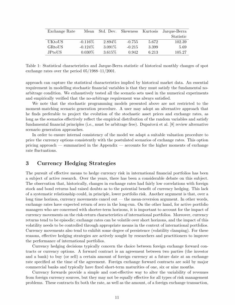
We analyze the statistical characteristics of exchange rates over the period 05/1988–11/2001 thatwere used in the static and dynamic tests. As can be seen in Table 1, the monthly variations of spotexchange rates exhibit skewed distributions. They also exhibit considerable variance in comparisonto their mean, as well as excess kurtosis, implying heavier tails than the normal distribution. Jarque-Berra tests [12] on these data indicate that normality hypotheses cannot be accepted.1

The skewed and leptokurtic distributions of the financial random variables (asset returns andexchange rates) motivated our choice of the moment-matching scenario generation procedure as this

1The Jarque-Berra statistic has a X 2 distribution with two degrees of freedom. Its critical values at the 5% and 1%confidence levels are 5.99 and 9.21, respectively. The normality hypothesis is rejected when the Jarque-Berra statistichas a higher value than the corresponding critical value at the respective confidence level.

10

Exchange Rate Mean Std. Dev. Skewness Kurtosis Jarque-BerraStatistic

UKtoUS -0.116% 2.894% -0.755 5.672 102.39GRtoUS -0.124% 3.091% -0.215 3.399 5.69JPtoUS 0.030% 3.615% 0.942 6.213 105.27

Table 1: Statistical characteristics and Jarque-Berra statistic of historical monthly changes of spotexchange rates over the period 05/1988–11/2001.

approach can capture the statistical characteristics implied by historical market data. An essentialrequirement in modelling stochastic financial variables is that they must satisfy the fundamental no-arbitrage condition. We exhaustively tested all the scenario sets used in the numerical experimentsand empirically verified that the no-arbitrage requirement was always satisfied.

We note that the stochastic programming models presented above are not restricted to themoment-matching scenario generation procedure. A user may adopt an alternative approach thathe finds preferable to project the evolution of the stochastic asset prices and exchange rates, aslong as the scenarios effectively reflect the empirical distribution of the random variables and satisfyfundamental financial principles (i.e., must be arbitrage free). Dupacova et al. [8] review alternativescenario generation approaches.

In order to ensure internal consistency of the model we adapt a suitable valuation procedure toprice the currency options consistently with the postulated scenarios of exchange rates. This optionpricing approach — summarized in the Appendix — accounts for the higher moments of exchangerate fluctuations.

3 Currency Hedging Strategies

The pursuit of effective means to hedge currency risk in international financial portfolios has beena subject of active research. Over the years, there has been a considerable debate on this subject.The observation that, historically, changes in exchange rates had fairly low correlations with foreignstock and bond returns had raised doubts as to the potential benefit of currency hedging. This lackof a systematic relationship could, in principle, lower portfolio risk. Another argument is that, over along time horizon, currency movements cancel out — the mean-reversion argument. In other words,exchange rates have expected return of zero in the long-run. On the other hand, for active portfoliomanagers who are concerned with shorter-term horizons, it is important to account for the impact ofcurrency movements on the risk-return characteristics of international portfolios. Moreover, currencyreturns tend to be episodic; exchange rates can be volatile over short horizons, and the impact of thisvolatility needs to be controlled through appropriate means in the context of international portfolios.Currency movements also tend to exhibit some degree of persistence (volatility clamping). For thesereasons, effective hedging strategies are actively sought by researchers and practitioners to improvethe performance of international portfolios.

Currency hedging decisions typically concern the choice between foreign exchange forward con-tracts or currency options. A forward contract is an agreement between two parties (the investorand a bank) to buy (or sell) a certain amount of foreign currency at a future date at an exchangerate specified at the time of the agreement. Foreign exchange forward contracts are sold by majorcommercial banks and typically have fixed short-term maturities of one, six or nine months.

Currency forwards provide a simple and cost-effective way to alter the variability of revenuesfrom foreign currency sources, but they may not be equally effective for all types of risk managementproblems. These contracts fix both the rate, as well as the amount, of a foreign exchange transaction,

11

and thus protect the value of a certain amount in foreign currency against a potential reduction inthe exchange rate. If the amount of foreign revenues is known with certainty, then an equivalentcurrency forward contract will completely eliminate the currency risk. However, in the case of foreignholdings of financial assets, their final value is stochastic due to their uncertain returns during theinterim period; hence, full hedging is not attainable in this case. A limitation of currency forwards isthat by fixing the exchange rate they forgo the opportunity for gains in the event that the exchangerate appreciates. One could argue that mitigating risk should be the primary consideration, whilepotential benefits from favorable exchange rate movements should be of a secondary concern. Butit is the entire risk-return tradeoff that usually guides portfolio management decisions.

Options provide alternative means to control risks. An exporter could “shell” his future foreignexchange receipts by purchasing a currency put. A portfolio manager could protect his foreign as-set holdings by buying currency options to mitigate currency risk exposure associated with foreigninvestments in the portfolio. Currency put options protect from losses in the event of a significantdrop in the exchange rate, but with no sacrifice of potential benefits in the event of currency appre-ciation, as they would simply not be exercised in such a case. However, currency options entail acost (purchase price).

In this study we experiment with two different trading strategies involving currency options thathave different payoff profiles.

Using Protective Put Options

By buying a European put currency option, the investor acquires the discretionary right to sella certain amount of foreign currency at a specified rate (exercise price) at the option’s maturitydate. In the numerical tests we consider protective put options for each foreign currency with threedifferent strike prices, Kj , (“in-the-money, ITM, “at-the-money”, ATM, and “out-of-the-money”,OTM). These three options constitute the set of available options, Jc, for each foreign currencyc ∈ C. The options have a term (maturity) of one-month that matches the duration of each decisionstage in the model. The ATM options have strike prices equal to the respective spot exchange ratesat the time of issue. As decisions are considered at non-leaf nodes of the scenario tree, the strikeprices of the ATM options are equal to the scenario-dependent spot exchange rates specified for thecorresponding node of the scenario tree. The ITM and OTM put options have strike prices thatare 5% higher, respectively 5% lower, than the corresponding spot exchange rates at the respectivedecision state. These levels of option strike prices have been chosen fairly arbitrarily. Obviously, alarger set of options with different strike prices and cost can be easily included in the model.

The model is allowed to take only long positions in the protective put options. Thus, we addnon-negativity constraints for the positions in options in model (2):

npcnc,j ≥ 0 , ∀ j ∈ Jc , ∀ c ∈ C , ∀n ∈ N \NT

Obviously, the OTM put option has a lower price than the ATM put which, in turn, is cheaperthan the ITM put option. In the numerical tests we have observed that when the model selectsoptions in the portfolios, these are OTM put options — ITM and ATM options are never selectedin the solutions when they are considered together with OTM put options.

Using BearSpread Strategies

A BearSpread strategy is composed of two put options with the same expiration date. It involves along position in an ITM put and a short position in an OTM put. The strike prices of the constituentoptions are set as described above.

Let npcnc,ITM and npcn

c,OTM be the long position in the ITM and the short position in the OTMcurrency put option, respectively, constituting a BearSpread position in foreign currency c ∈ C at

12

decision node n ∈ N \NT . To incorporate the BearSpeard strategy in the optimization model (2),we additionally impose the following constraints:

npcnc,OTM + npcn

c,ITM = 0 , ∀ c ∈ C , ∀n ∈ N \NT

npcnc,ITM ≥ 0 , ∀ c ∈ C , ∀n ∈ N \NT

The first constraint ensures that the positions in the respective put options have the same magnitude,while the second constraint ensures that the long position is in the ITM option.

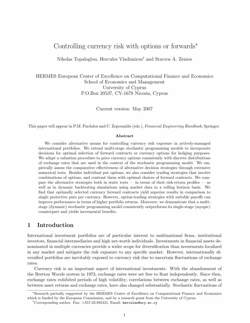
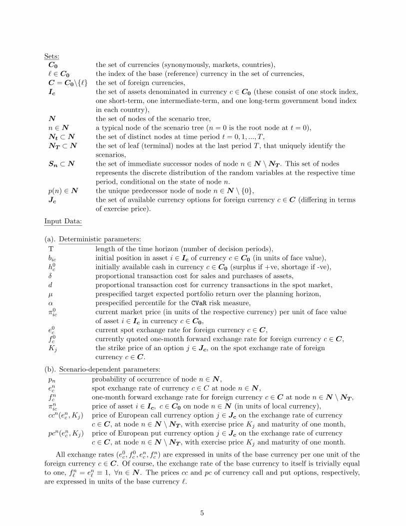
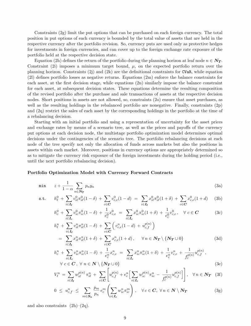
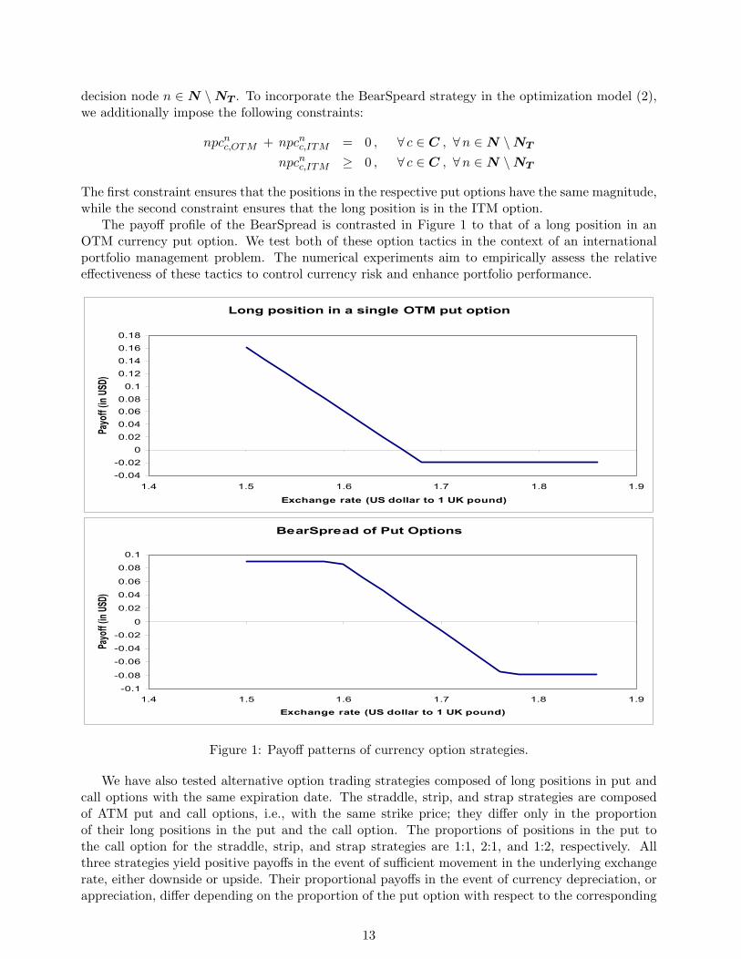
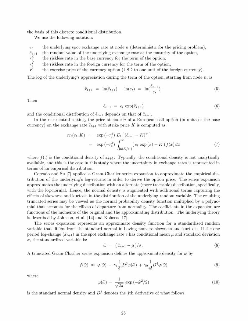
The payoff profile of the BearSpread is contrasted in Figure 1 to that of a long position in anOTM currency put option. We test both of these option tactics in the context of an internationalportfolio management problem. The numerical experiments aim to empirically assess the relativeeffectiveness of these tactics to control currency risk and enhance portfolio performance.

Long position in a single OTM put option

-0.04-0.02

00.020.040.060.080.10.120.140.160.18

1.4 1.5 1.6 1.7 1.8 1.9

Exchange rate (US dollar to 1 UK pound)

Payo

ff (in

USD)

BearSpread of Put Options

-0.1

-0.08

-0.06

-0.04

-0.02

0

0.02

0.04

0.06

0.08

0.1

1.4 1.5 1.6 1.7 1.8 1.9

Exchange rate (US dollar to 1 UK pound)

Payo

ff (in

USD)

Figure 1: Payoff patterns of currency option strategies.

We have also tested alternative option trading strategies composed of long positions in put andcall options with the same expiration date. The straddle, strip, and strap strategies are composedof ATM put and call options, i.e., with the same strike price; they differ only in the proportionof their long positions in the put and the call option. The proportions of positions in the put tothe call option for the straddle, strip, and strap strategies are 1:1, 2:1, and 1:2, respectively. Allthree strategies yield positive payoffs in the event of sufficient movement in the underlying exchangerate, either downside or upside. Their proportional payoffs in the event of currency depreciation, orappreciation, differ depending on the proportion of the put option with respect to the corresponding

13

call option. Although these strategies yield gains in the event of even moderate volatility in exchangerates, they have a higher cost as they are composed of ATM options. The strangle strategy involveslong positions (equal in magnitude) in an OTM put and an OTM call option. It provides coverageagainst larger movements of the underlying exchange rate, in comparison to the previous threestrategies, but at a lower cost.

We do not report results with these option trading strategies because in the numerical tests thestraddle, strip and strap strategies were dominated both by the forward contracts, as well as by theuse of a single protective OTM put option per currency. The performance of the strangle strategywas essentially indistinguishable from that of a single protective put per currency.

4 Empirical Results

As prior research suggests, currency risk is a main aspect of overall risk of international portfolios;controlling currency risk is important to enhance portfolio performance. We examine the effectivenessof alternative tactics to control the currency risk of international diversified portfolios of stock andbond indices. Alternative strategies, using either forward exchange contracts or currency options areevaluated and compared in terms of their performance in empirical tests using market data.

We solved single-stage and two-stage instances of the stochastic programming models describedin section 2. The results of the numerical tests enable a comparative assessment of the following:

• Forward exchange contracts versus currency options,

• Alternative tactics with currency options,

• Single-stage vs two-stage stochastic programming models.

First, we compare the performance of a single-stage model with forward contracts against thatof a corresponding model that uses currency options as means to mitigate currency risk. Second, wecompare the performance of alternative tactics that provide coverage against unfavorable movementsin exchange rates by means of currency options. Finally, we consider the performance of two-stagevariants of the stochastic programming models. The two-stage models permit rebalancing at an inter-mediate decision stage, at which currency options held may be exercised, and new option contractscan be purchased. We investigate the incremental improvements in performance of the internationalportfolios that can be achieved with the two-stage models, over their single-stage counterparts.

As explained in section 2, the models select internationally diversified portfolios of stock and bondindices, and appropriate positions in currency hedging instruments (forward contracts or currencyoptions), in order to minimize the excess downside risk while meeting a desirable target of expectedreturn. Selective hedging is the norm followed in all tests.

Performance comparisons are made with static tests (in terms of risk-return efficient frontiers), aswell as with dynamic tests. The dynamic tests involve backtesting experiments over a rolling horizonof 43 months: 04/1998–11/2001. At each month we use the historical data from the preceding tenyears to calibrate the scenario generation procedure: we calculate the four marginal moments andcorrelations of the random variables and use these estimates as the target statistics in the moment-matching scenario generation procedure. We price the respective currency options on the nodes ofthe scenario tree using the method described in the Appendix. The scenario tree of asset prices andexchange rates, and the option prices, are used as inputs to the portfolio optimization model. Eachmonth we solve one instance of the optimization model (single- or multi- stage) and record the optimalfirst-stage decisions. The clock is advanced one month and the market values of the random variablesare revealed. Based on these we determine the actual return using the composition of the portfolioat hand, the observed market prices for the assets and the exchange rates, and the payoffs from thediscretionary exercise of currency options that are held. We update the cash holdings accordingly.

14

Starting with the new initial portfolio composition we repeat the same procedure for the followingmonth. The ex post realized returns are compounded and analyzed over the entire simulation period.These reflect the portfolio returns that would have been obtained had the recommendations of therespective model been adopted during the simulation period.

We ran backtesting experiments for each investment tactic that is studied, using the CVaR metricto minimize excess shortfall in all cases.

4.1 Efficient Frontiers

We now examine the potential performance of forwards and currency options, in comparison to un-hedged portfolios, in terms of the risk-return profiles of their respective portfolios. Thus, we examinethe potential effects of currency hedging through alternative means by comparing the efficient fron-tiers resulting from the alternative decision tactics. Single-stage CVaR models were used for all testreported in this section.

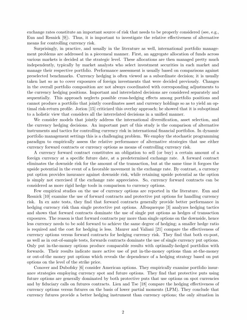
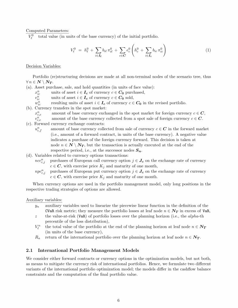
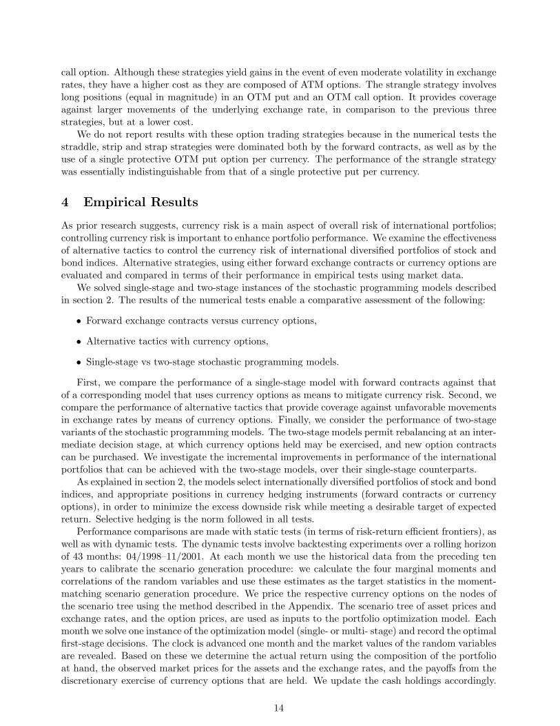
Figure 2 contrasts the efficient frontiers of CVaR-optimized international portfolios on August 2001using optimal positions in currency options or forward contracts, versus totally unhedged portfolios.We consider two different strategies with currency options: (a) a single protective put option (“at-the-money”, “in-the-money” or “out-of-the-money”), (b) a BearSpread strategy of put options.

Efficient frontiers of international portfolioswith different hedging strategies (Aug.2001)

0.40%

0.50%

0.60%

0.70%

0.80%

0.90%

1.00%

1.10%

1.20%

0 0.02 0.04 0.06 0.08 0.1 0.12 0.14 0.16CVaR (95%) of Portfolio Losses

Exp

ecte

d R

etu

rn (

mo

nth

ly)

UnhedgedForward ContractsATM put optionOTM put optionBearSpread options

Figure 2: Efficient frontiers of CVaR-optimized international portfolios of stock and bond indices, andcurrency hedging instruments.

15

We observe that risk-return efficient frontiers of hedged portfolios (using either forwards or cur-rency options) clearly dominate the efficient frontiers of unhedged portfolios. The efficient frontiersof unhedged portfolios extend into a range of higher risk levels. Clearly, the selectively hedged port-folios are preferable to unhedged portfolios; at any level of expected return, efficient hedged portfolioshave a substantially lower level of risk — as measured by the CVaR metric — compared to efficientunhedged portfolios. We also observe that currency risk hedging (regardless of the strategy used)yields higher benefits, in terms of higher expected returns compared to the unhedged case, for themedium and high risk portfolios, rather than for the low risk portfolios. The potential gain from riskreduction is increasing for more aggressive targets of expected portfolio returns.

These ex ante results indicate that forward contracts exhibit superior potential as hedging instru-ments compared to currency options. The results in Figure 2 show that, while the various strategiesof currency options produce efficient frontiers that dominate that of the unhedged portfolios, themost dominant efficient frontier is the one produced with the optimal selection of forward contracts.For any value of target expected return, the optimal hedged portfolios with forwards exhibit a lowerlevel of risk than the efficient portfolios of any other strategy. The use of currency options improvesthe performance of international portfolios compared to unhedged portfolios, but forward contractsexhibit the most dominant performance in the static tests.

Among the trading strategies using currency options, we observe that the efficient frontier with“out-of-the-money” options is the closest to that obtained with forward contracts, especially in thehighest levels of target expected return (i.e., most aggressive investment cases). The efficient frontierof the BearSpread strategy follows next, but the differences from the first two are increasing for moreaggressive targets of expected portfolio returns. Portfolios with “in-the-money” or “at-the-money”options give almost indistinguishable risk-return efficient frontiers.

4.2 Dynamic Tests: Ex-post Comparative Performance of Portfolios with Cur-rency Options

The results of the previous section indicate that, in static tests, forward contracts demonstratedbetter ex ante performance potential compared to currency options. We additionally ran a numberof backtesting experiments on a rolling horizon basis for a more substantive empirical assessment ofalternative currency hedging strategies.

Single-Stage Models

First, we compare the ex post realized performance of portfolios with various hedging strategies thatare incorporated in single-stage stochastic programming models. The models have a holding periodof one month, and consider portfolio restructuring decisions at a single point during the planninghorizon. The joint distribution of the random variables (asset returns and exchange rates) duringthe one-month horizon of the models is represented by sets of 15,000 discrete scenarios.

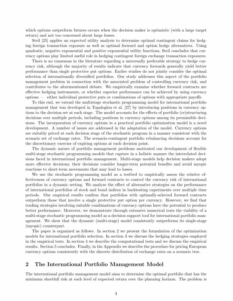
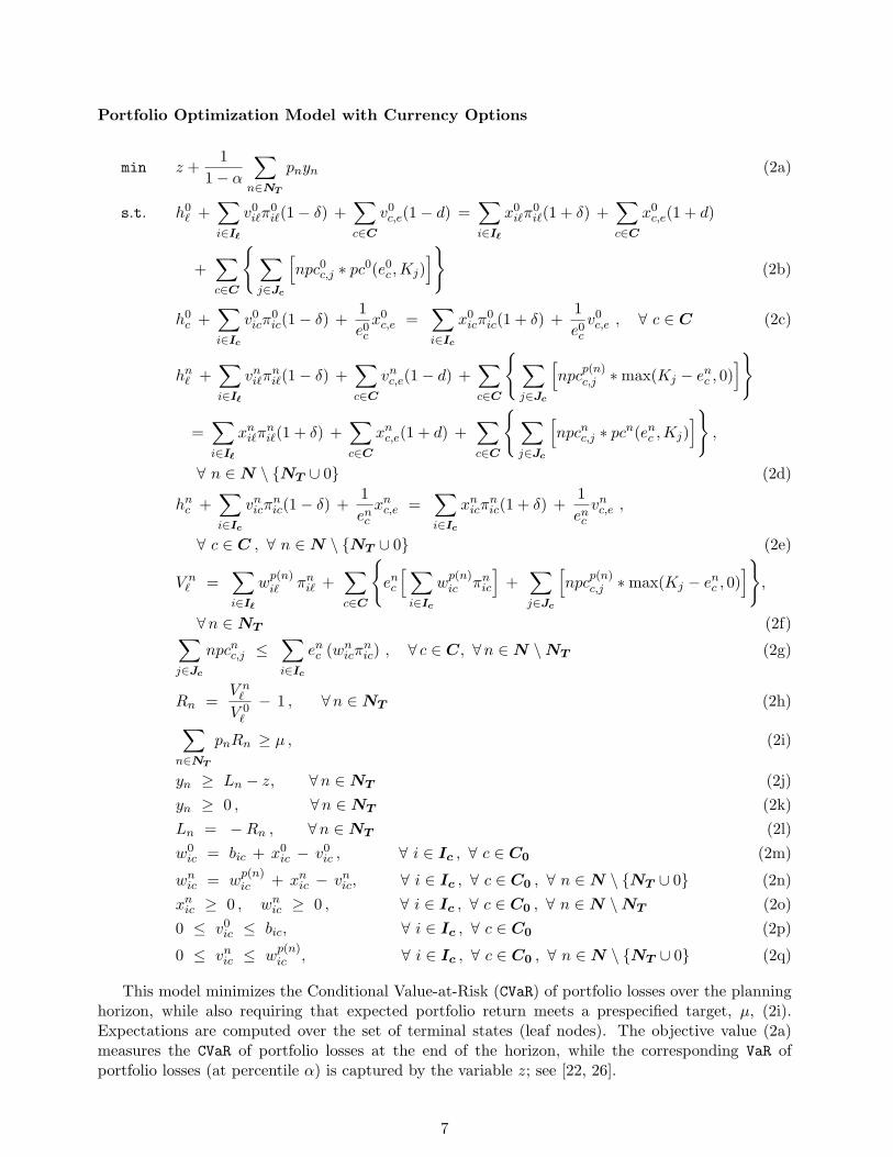
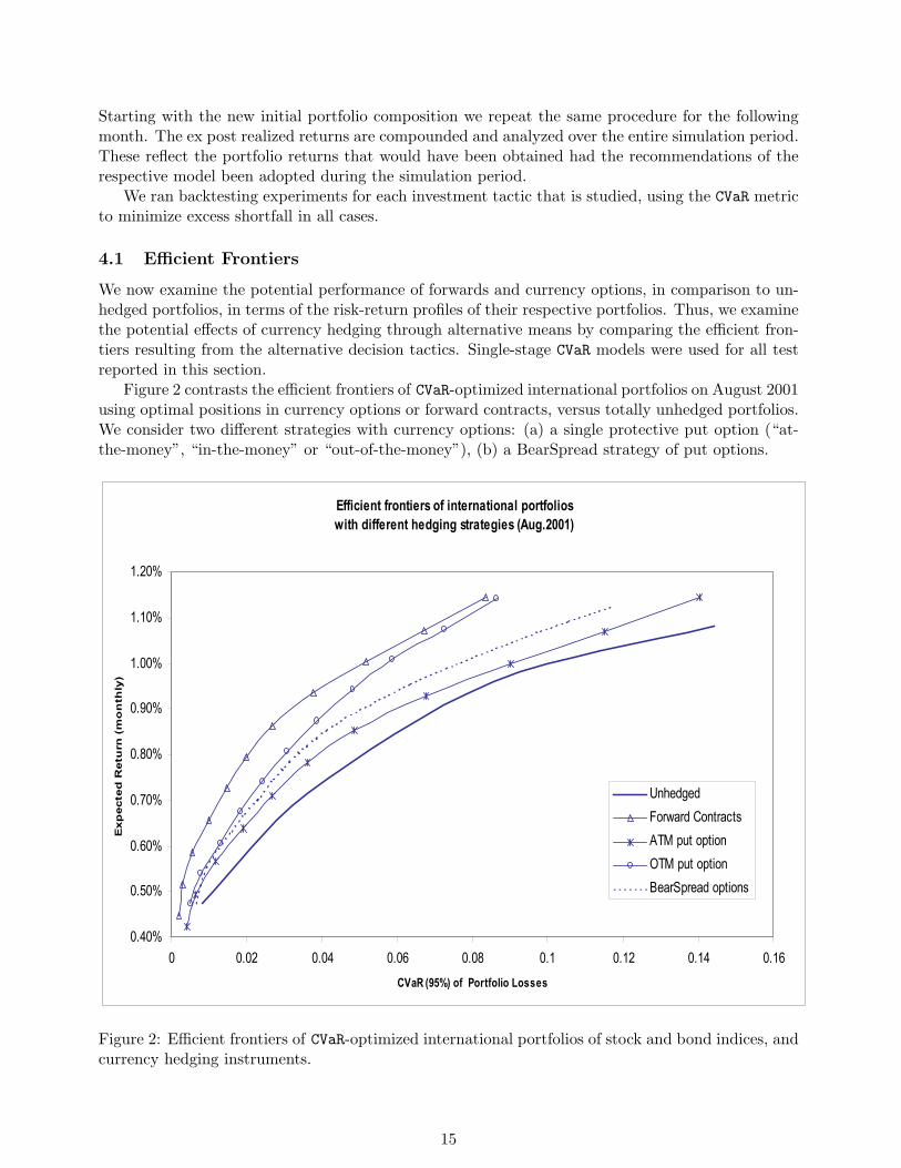
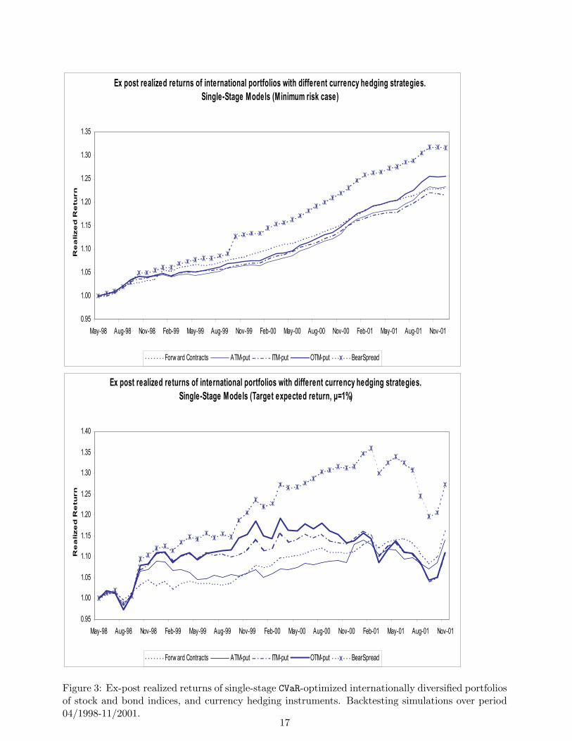
Figure 3 contrasts the ex post performance of portfolios with optimal forward contracts with thatof portfolios using different strategies of put options. The first graph compares performance in theminimum risk case — i.e., when the models simply minimize the CVaR risk measure at the end of theplanning horizon, without imposing any minimal target on expected portfolio return; for the secondgraph the target expected return during the one-month planning horizon is µ = 1%.

We observe that in the minimum risk case of the dynamic tests, forward contracts and the use ofa single protective put per currency resulted in very similar performance, regardless of the exerciseprice of the options (i.e., ITM, ATM or OTM). Forward contracts exhibited the most stable returnpath throughout the simulation period, indicating their effectiveness in hedging currency risk. Inthis minimum risk case, the models did not select a large number of currency options, resulting inlow hedge ratios.

16

Ex post realízed returns of international portfolios with different currency hedging strategies. Single-Stage Models (Minimum risk case)

0.95

1.00

1.05

1.10

1.15

1.20

1.25

1.30

1.35

May-98 Aug-98 Nov-98 Feb-99 May-99 Aug-99 Nov-99 Feb-00 May-00 Aug-00 Nov-00 Feb-01 May-01 Aug-01 Nov-01

Re

alize

d R

etu

rn

Forw ard Contracts ATM-put ITM-put OTM-put BearSpread

Ex post realízed returns of international portfolios with different currency hedging strategies. Single-Stage Models (Target expected return, µ=1%)

0.95

1.00

1.05

1.10

1.15

1.20

1.25

1.30

1.35

1.40

May-98 Aug-98 Nov-98 Feb-99 May-99 Aug-99 Nov-99 Feb-00 May-00 Aug-00 Nov-00 Feb-01 May-01 Aug-01 Nov-01

Re

alize

d R

etu

rn

Forw ard Contracts ATM-put ITM-put OTM-put BearSpread

Figure 3: Ex-post realized returns of single-stage CVaR-optimized internationally diversified portfoliosof stock and bond indices, and currency hedging instruments. Backtesting simulations over period04/1998-11/2001.

17

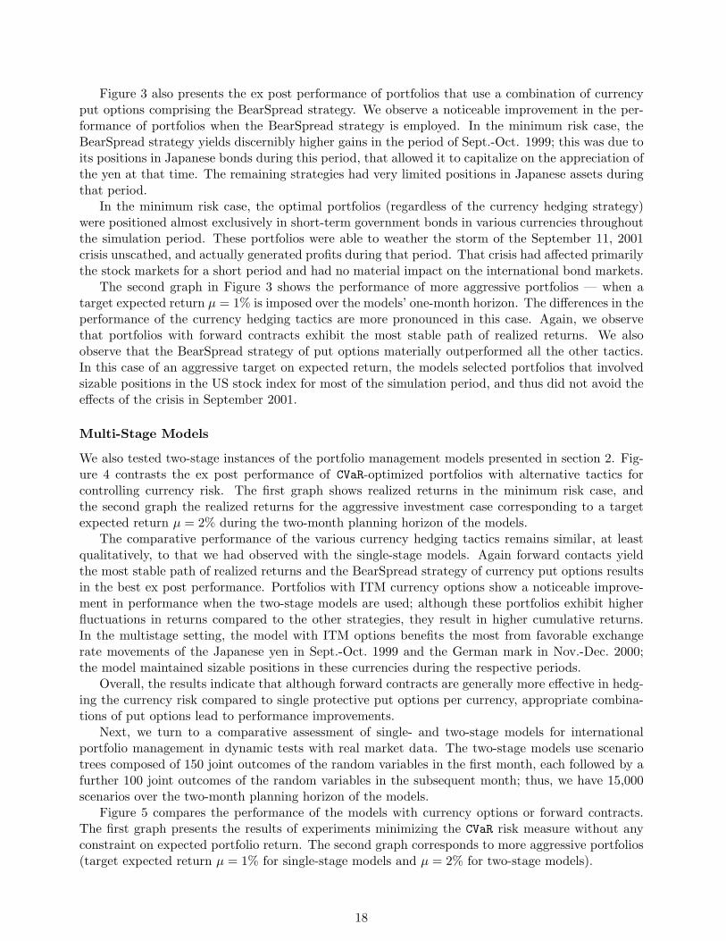
Figure 3 also presents the ex post performance of portfolios that use a combination of currencyput options comprising the BearSpread strategy. We observe a noticeable improvement in the per-formance of portfolios when the BearSpread strategy is employed. In the minimum risk case, theBearSpread strategy yields discernibly higher gains in the period of Sept.-Oct. 1999; this was due toits positions in Japanese bonds during this period, that allowed it to capitalize on the appreciation ofthe yen at that time. The remaining strategies had very limited positions in Japanese assets duringthat period.

In the minimum risk case, the optimal portfolios (regardless of the currency hedging strategy)were positioned almost exclusively in short-term government bonds in various currencies throughoutthe simulation period. These portfolios were able to weather the storm of the September 11, 2001crisis unscathed, and actually generated profits during that period. That crisis had affected primarilythe stock markets for a short period and had no material impact on the international bond markets.

The second graph in Figure 3 shows the performance of more aggressive portfolios — when atarget expected return µ = 1% is imposed over the models’ one-month horizon. The differences in theperformance of the currency hedging tactics are more pronounced in this case. Again, we observethat portfolios with forward contracts exhibit the most stable path of realized returns. We alsoobserve that the BearSpread strategy of put options materially outperformed all the other tactics.In this case of an aggressive target on expected return, the models selected portfolios that involvedsizable positions in the US stock index for most of the simulation period, and thus did not avoid theeffects of the crisis in September 2001.

Multi-Stage Models

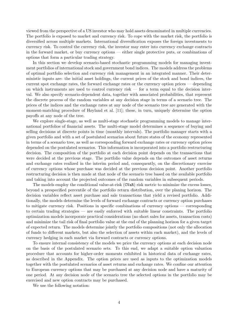
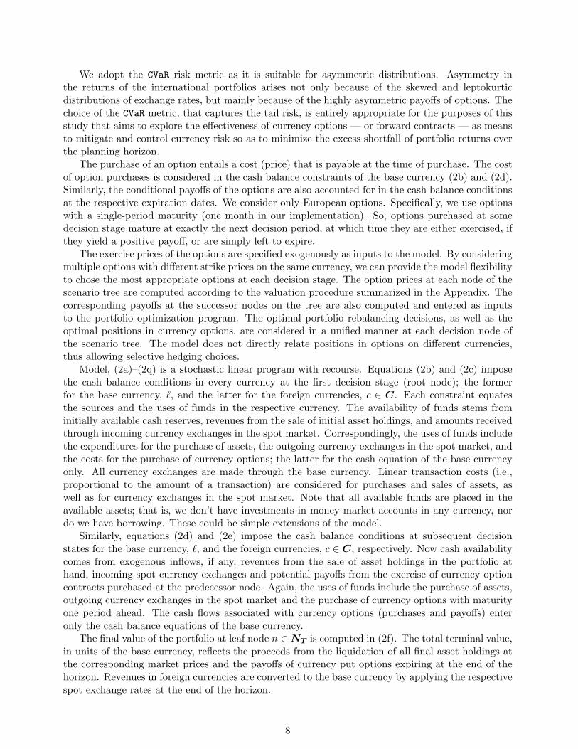
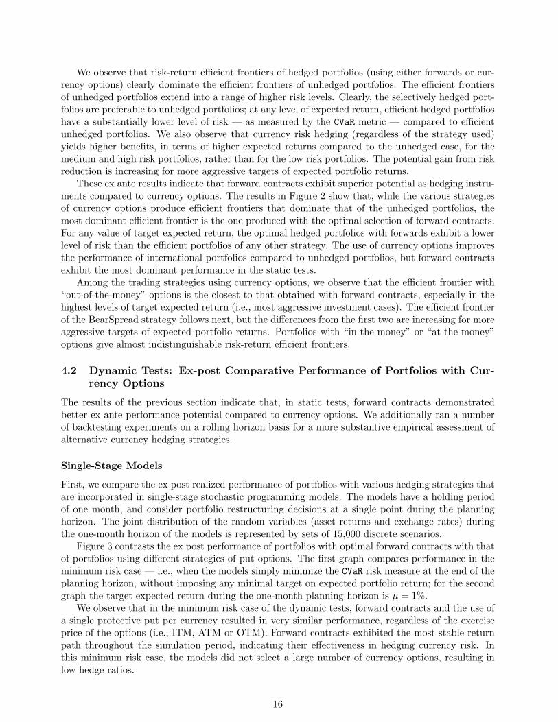
We also tested two-stage instances of the portfolio management models presented in section 2. Fig-ure 4 contrasts the ex post performance of CVaR-optimized portfolios with alternative tactics forcontrolling currency risk. The first graph shows realized returns in the minimum risk case, andthe second graph the realized returns for the aggressive investment case corresponding to a targetexpected return µ = 2% during the two-month planning horizon of the models.

The comparative performance of the various currency hedging tactics remains similar, at leastqualitatively, to that we had observed with the single-stage models. Again forward contacts yieldthe most stable path of realized returns and the BearSpread strategy of currency put options resultsin the best ex post performance. Portfolios with ITM currency options show a noticeable improve-ment in performance when the two-stage models are used; although these portfolios exhibit higherfluctuations in returns compared to the other strategies, they result in higher cumulative returns.In the multistage setting, the model with ITM options benefits the most from favorable exchangerate movements of the Japanese yen in Sept.-Oct. 1999 and the German mark in Nov.-Dec. 2000;the model maintained sizable positions in these currencies during the respective periods.

Overall, the results indicate that although forward contracts are generally more effective in hedg-ing the currency risk compared to single protective put options per currency, appropriate combina-tions of put options lead to performance improvements.

Next, we turn to a comparative assessment of single- and two-stage models for internationalportfolio management in dynamic tests with real market data. The two-stage models use scenariotrees composed of 150 joint outcomes of the random variables in the first month, each followed by afurther 100 joint outcomes of the random variables in the subsequent month; thus, we have 15,000scenarios over the two-month planning horizon of the models.

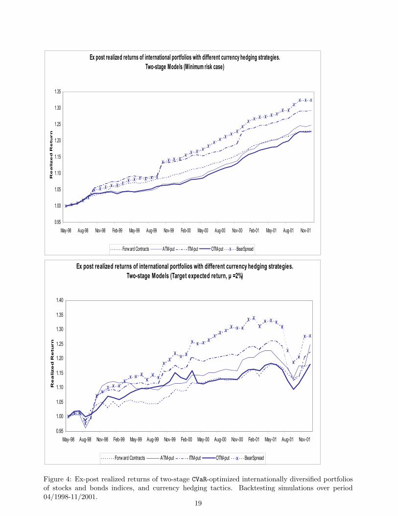
Figure 5 compares the performance of the models with currency options or forward contracts.The first graph presents the results of experiments minimizing the CVaR risk measure without anyconstraint on expected portfolio return. The second graph corresponds to more aggressive portfolios(target expected return µ = 1% for single-stage models and µ = 2% for two-stage models).

18

Ex post realízed returns of international portfolios with different currency hedging strategies. Τwo-stage Models (Minimum risk case)

0.95

1.00

1.05

1.10

1.15

1.20

1.25

1.30

1.35

May-98 Aug-98 Nov-98 Feb-99 May-99 Aug-99 Nov-99 Feb-00 May-00 Aug-00 Nov-00 Feb-01 May-01 Aug-01 Nov-01

Re

alize

d R

etu

rn

Forw ard Contracts ATM-put ITM-put OTM-put BearSpread

Ex post realízed returns of international portfolios with different currency hedging strategies. Two-stage Models (Target expected return, µ =2%)

0.95

1.00

1.05

1.10

1.15

1.20

1.25

1.30

1.35

1.40

May-98 Aug-98 Nov-98 Feb-99 May-99 Aug-99 Nov-99 Feb-00 May-00 Aug-00 Nov-00 Feb-01 May-01 Aug-01 Nov-01

Re

alize

d R

etu

rn

Forw ard Contracts ATM-put ITM-put OTM-put BearSpread

Figure 4: Ex-post realized returns of two-stage CVaR-optimized internationally diversified portfoliosof stocks and bonds indices, and currency hedging tactics. Backtesting simulations over period04/1998-11/2001.

19

Ex post realized returns with single- and two-stage models(Minimum risk case)

0.95

1.00

1.05

1.10

1.15

1.20

1.25

1.30

1.35

May-98 Aug-98 Nov-98 Feb-99 May-99 Aug-99 Nov-99 Feb-00 May-00 Aug-00 Nov-00 Feb-01 May-01 Aug-01 Nov-01

Re

alize

d R

etu

rn

Forw ard_Single Forw ard_Tw oStage ITM_Single ITM_Tw oStage BearSpread_Single BearSpread_Tw oStage

Ex post realized returns with single- (µ=1%) and two-stage (µ=2%) models

0.95

1.00

1.05

1.10

1.15

1.20

1.25

1.30

1.35

1.40

May-98 Aug-98 Nov-98 Feb-99 May-99 Aug-99 Nov-99 Feb-00 May-00 Aug-00 Nov-00 Feb-01 May-01 Aug-01 Nov-01

Re

alize

d R

etu

rn

Forw ard_Single Forw ard_Tw oStage ITM_Single ITM_Tw oStage BearSpread_Single BearSpread_Tw oStage

Figure 5: Ex-post realized returns of CVaR-optimized international portfolios of stocks and bondindices, and currency hedging tactics. Comparison of single- and two-stage models.

20

We observe that in the minimum risk case the models exhibit stable portfolio returns throughoutthe simulation period, with small losses in only very few periods. The more aggressive cases exhibitlarger fluctuations in returns, reflecting riskier portfolios. In Figure 5 we observe that when currencyrisk is hedged with forward contracts, the two-stage model gives only slightly better results comparedto the single-stage model. However, when currency options are used, the performance improvementsof the two-stage models compared to the corresponding single-stage models are more evident, par-ticularly for the cases that use ITM put options. Performance improvements with the two-stagemodel are also observed when the BearSpread strategy is employed. In all tests, and regardless ofthe trading strategy of options that is used, the two-stage models result in improved performancecompared to the corresponding single-stage models.

In comparison to their single-stage counterparts, two-stage models incorporate the followingadvantages: (a) a longer planning horizon that permits to assess the sustained effects of investmentchoices, (b) increased information content as it accounts for the evolution of the random variablesover the longer planning horizon, (c) the opportunity to account for the effect of portfolio rebalancingat an intermediate point during the planning horizon. The combined effects of these features lead tothe selection of more effective portfolios with the two-stage models. The performance improvementsare evident in higher and more stable portfolio returns that are achieved with the two-stage modelsin comparison to their single-stage counterparts.

Empirical comparisons of multi-stage stochastic programming models and single-stage modelsare scantly found in the literature. The results of this study demonstrate the performance improve-ments that are achievable with the adoption of multi-stage stochastic programs — that account forinformation and decision dynamics — in comparison to single-stage (myopic) models.

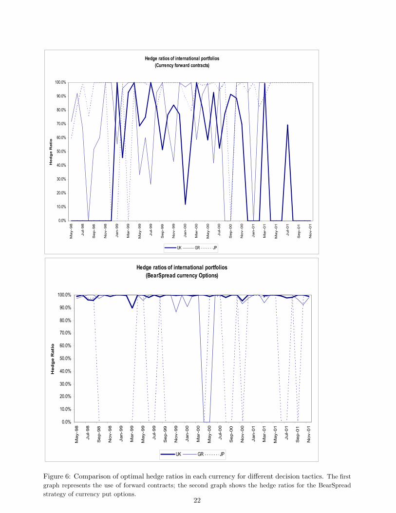
Figure 6 shows the degree of currency hedging in each country (% of foreign investments hedged),when using forward contracts or currency options that form the BearSpread strategy to controlcurrency risk; these results correspond to the first-stage decisions of the two-stage optimizationmodels. The differences are evident. When using currency options, the model consistently choosesto hedge to a high degree — hedge ratios between 90% and 100% — foreign investments in theselected portfolios (see the second graph in Fig. 6). The hedge ratio is zero only when the selectedportfolio does not include asset holdings in a particular foreign market. The degree of hedging isevidently different when forward contracts are used to control currency risk (first graph in Fig. 6).In this case the model makes much more use of the selective hedging flexibility; hedge ratios varyingboth in magnitude as well as across currencies are observed during the simulation period. Moreover,we have observed that, in comparison to the single-stage models, the two-stage models select morediversified portfolios throughout the simulation period and exhibit lower portfolio turnover.

Finally, we compute some measures to compare the overall performance of the models. Specifi-cally, we consider the following measures of the exp-post realized monthly returns over the simulationperiod: geometric mean, standard deviation, Sharpe ratio and the upside potential and downsiderisk ratio (UPratio) proposed by Sortino and van der Meer [24]). This ratio contrasts the upsidepotential against a specific benchmark with the shortfall risk against the same benchmark. We usethe risk-free rate of one-month T-bills as the benchmark. This ratio is computed as follows. Let rt

be the realized return of a portfolio in month t = 1, . . . , k of the simulation, where k = 43 is thenumber of months in the simulation period 04/1998−11/2001. Let ρt be the return of the benchmark(riskless asset) at the same period. Then the UPratio is

UPratio =1k

∑kt=1 max [0, rt − ρt]

[ 1k∑k

t=1( max [0, rt − ρt] )2]1/2(4)

The numerator is the average excess return compared to the benchmark, reflecting the upsidepotential. The denominator is a measure of downside risk, as proposed in Sortino et al. [23], and canbe thought of as the risk of failing to meet the benchmark.

21

Hedge ratios of international portfolios (Currency forward contracts)

0.0%

10.0%

20.0%

30.0%

40.0%

50.0%

60.0%

70.0%

80.0%

90.0%

100.0%

May-98

Jul-98

Sep-98

Nov-98

Jan-99

Mar-99

May-99

Jul-99

Sep-99

Nov-99

Jan-00

Mar-00

May-00

Jul-00

Sep-00

Nov-00

Jan-01

Mar-01

May-01

Jul-01

Sep-01

Nov-01

Hed

ge R

ati

o

UK GR JP

Hedge ratios of international portfolios (BearSpread currency Options)

0.0%

10.0%

20.0%

30.0%

40.0%

50.0%

60.0%

70.0%

80.0%

90.0%

100.0%

May-98

Jul-98

Sep-98

Nov-98

Jan-99

Mar-99

May-99

Jul-99

Sep-99

Nov-99

Jan-00

Mar-00

May-00

Jul-00

Sep-00

Nov-00

Jan-01

Mar-01

May-01

Jul-01

Sep-01

Nov-01

Hed

ge

Rat

io

UK GR JP

Figure 6: Comparison of optimal hedge ratios in each currency for different decision tactics. The firstgraph represents the use of forward contracts; the second graph shows the hedge ratios for the BearSpreadstrategy of currency put options.

22

Statistic forwards ITM ATM OTM BearSpreadcontracts put put put strategy

Statistics of monthly realized returns, single-stage model (µ = 1%)Geometric Mean 0.0043 0.0035 0.0021 0.0022 0.0057Stand. Dev. 0.0139 0.0148 0.0193 0.0222 0.0205Sharpe Ratio -0.0307 -0.0808 -0.1324 -0.1128 0.0468UPratio 0.9500 0.8800 0.6910 0.7060 0.8300Statistics of monthly realized returns, single-stage model (minimum risk)Geometric Mean 0.0057 0.0058 0.0054 0.0063 0.0076Stand. Dev. 0.0027 0.0045 0.0036 0.0042 0.0061Sharpe Ratio 0.3796 0.2350 0.1911 0.3641 0.4725UPratio 11.1355 5.4853 6.7168 6.7518 25.1671Statistics of monthly realized returns, two-stage model (µ = 2%)Geometric Mean 0.0046 0.0061 0.0056 0.0045 0.0065Stand. Dev. 0.0124 0.0163 0.0193 0.0153 0.0208Sharpe Ratio -0.0120 0.0862 0.0458 -0.1023 0.0864UPratio 0.9690 0.9470 0.7670 0.8380 0.833Statistics of monthly realized returns, two-stage model (minimum risk)Geometric Mean 0.0058 0.0061 0.0071 0.0057 0.0078Stand. Dev. 0.0025 0.0047 0.0078 0.0042 0.0075Sharpe Ratio 0.4132 0.3006 0.3083 0.2302 0.4108UPratio 12.4510 5.4270 10.1260 4.6344 21.134

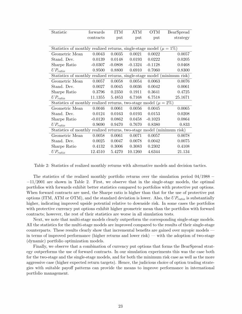
Table 2: Statistics of realized monthly returns with alternative models and decision tactics.

The statistics of the realized monthly portfolio returns over the simulation period 04/1988 −−11/2001 are shown in Table 2. First, we observe that in the single-stage models, the optimalportfolios with forwards exhibit better statistics compared to portfolios with protective put options.When forward contracts are used, the Sharpe ratio is higher than that for the use of protective putoptions (ITM, ATM or OTM), and the standard deviation is lower. Also, the UPratio is substantiallyhigher, indicating improved upside potential relative to downside risk. In some cases the portfolioswith protective currency put options exhibit higher geometric mean than the portfolios with forwardcontracts; however, the rest of their statistics are worse in all simulation tests.

Next, we note that multi-stage models clearly outperform the corresponding single-stage models.All the statistics for the multi-stage models are improved compared to the results of their single-stagecounterparts. These results clearly show that incremental benefits are gained over myopic models —in terms of improved performance (higher returns and lower risk) — with the adoption of two-stage(dynamic) portfolio optimization models.

Finally, we observe that a combination of currency put options that forms the BearSpread strat-egy outperforms the use of forward contracts. In our simulation experiments this was the case bothfor the two-stage and the single-stage models, and for both the minimum risk case as well as the moreaggressive case (higher expected return targets). Hence, the judicious choice of option trading strate-gies with suitable payoff patterns can provide the means to improve performance in internationalportfolio management.

23

5 Conclusions

This paper investigated alternative strategies for controlling currency risk in international portfoliosof financial assets. We carried out extensive numerical tests using market data to empirically assessthe effectiveness of alternative means for controlling currency risk in international portfolios.

Empirical results indicate that the optimal choice of forward contracts outperforms the use ofa single protective put option per currency. The results of both static, as well as dynamic, testsshow that optimal portfolios with forward contacts achieve better performance than portfolios withprotective put options. However, combinations of currency put options, like the BearSpread strategy,exhibit performance improvements. Yet, forward contracts consistently produced the more stablereturns in all simulation experiments.

Finally, we point out the notable performance improvements of international portfolios that resultfrom the adoption of dynamic (multi-stage) portfolio optimization models instead of the simpler, butmore restricted myopic (single-stage) models. The two-stage models tested in this study consistentlyoutperformed their single-stage counterparts in all cases (i.e., regardless of the decision tactics thatwere tested as means to control currency risk). These results strengthen the argument for the devel-opment, implementation and use of more sophisticated dynamic stochastic programming models forportfolio management. These models are more complex, have higher information demands (i.e., com-plete scenario trees), and are computationally more demanding because of their significantly largersize. However, as the results of this study demonstrate, dynamic models yield superior solutions,that is, more effective portfolios that attain higher returns and lower risk. Such improvements areimportant in an increasingly competitive financial environment.

The next step of this work is to investigate the use of appropriate instruments and decisiontactics, in the context of dynamic stochastic programming models, so as to jointly control multiplerisks that are encountered in international portfolio management. For example, we can incorporatein the models options on stocks as means to control market risk in addition to forward exchangecontracts or currency options to control currency risk. We expect that such an approach to jointlymanage all risk factors in the problem should yield additional benefits.

6 Appendix: Pricing Currency Options

In order to incorporate currency options in the stochastic programming model and maintain internalconsistency, the options must be priced in accordance with the discrete distributions of the underlyingas represented by the scenario tree. Conventional option pricing methods are not applicable as theyrely on specific distributional assumptions on the underlying that are not satisfied in this case. Inthis study, the scenarios of asset returns and exchange rates are generated with a moment-matchingmethod so as to closely reflect the empirical distributions of the random variables implied by historicalmarket data.

We price the currency options based on empirical distributions of the exchange rates using avaluation procedure developed by Corrado and Su [7], based on an idea of approximating the densityof the underlying by a series expansion that was introduced by Jarrow and Rudd [13]. Backus etal. [4] extended this approach to price currency options; we adapt their methodology.

We consider European currency options with maturity equaling a single period of the portfoliooptimization model (i.e., one month). To price such a European option at a non-terminal node (state)n ∈ N \NT of the scenario tree, the essential inputs are: the price of the underlying (exchange rate)at the option’s issue date (i.e., at node n) and the distribution of the underlying at the maturitydate, conditional on the state at the issue date (i.e., conditional on state n). In the context of ascenario tree, this conditional distribution is represented by the discrete outcomes of the underlyingassociated with the immediate successor nodes (set Sn) of node n. Hence, the option is priced on

24

the basis of this discrete conditional distribution.We use the following notation:

et the underlying spot exchange rate at node n (deterministic for the pricing problem),et+1 the random value of the underlying exchange rate at the maturity of the option,rdt the riskless rate in the base currency for the term of the option,

rft the riskless rate in the foreign currency for the term of the option,

K the exercise price of the currency option (USD to one unit of the foreign currency).

The log of the underlying’s appreciation during the term of the option, starting from node n, is

xt+1 = ln(et+1) − ln(et) = ln(et+1

et) . (5)

Thenet+1 = et exp(xt+1) (6)

and the conditional distribution of et+1 depends on that of xt+1.In the risk-neutral setting, the price at node n of a European call option (in units of the base

currency) on the exchange rate et+1 with strike price K is computed as:

cct(et,K) = exp (−rdt ) Et

[(et+1 −K)+

]= exp (−rd

t )∫ ∞

ln(K/et)( et exp (x)−K ) f(x) dx (7)

where f(.) is the conditional density of xt+1. Typically, the conditional density is not analyticallyavailable, and this is the case in this study where the uncertainty in exchange rates is represented interms of an empirical distribution.

Corrado and Su [7] applied a Gram-Charlier series expansion to approximate the empirical dis-tribution of the underlying’s log-returns in order to derive the option price. The series expansionapproximates the underlying distribution with an alternate (more tractable) distribution, specifically,with the log-normal. Hence, the normal density is augmented with additional terms capturing theeffects of skewness and kurtosis in the distribution of the underlying random variable. The resultingtruncated series may be viewed as the normal probability density function multiplied by a polyno-mial that accounts for the effects of departure from normality. The coefficients in the expansion arefunctions of the moments of the original and the approximating distribution. The underlying theoryis described by Johnson, et al. [14] and Kolassa [17].

The series expansion represents an approximate density function for a standardized randomvariable that differs from the standard normal in having nonzero skewness and kurtosis. If the oneperiod log-change (xt+1) in the spot exchange rate e has conditional mean µ and standard deviationσ, the standardized variable is:

ω = ( xt+1 − µ )/σ . (8)

A truncated Gram-Charlier series expansion defines the approximate density for ω by

f(ω) ≈ ϕ(ω) − γ113!

D3ϕ(ω) + γ214!

D4ϕ(ω) (9)

whereϕ(ω) =

1√2π

exp (−ω2/2) (10)

is the standard normal density and Dj denotes the jth derivative of what follows.

25

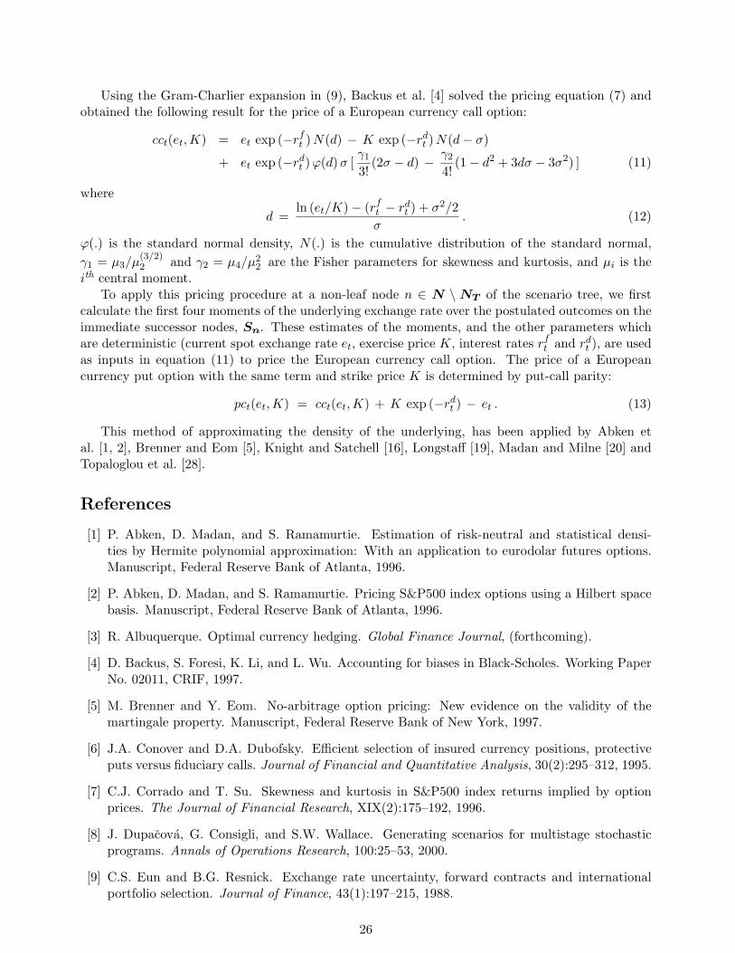
Using the Gram-Charlier expansion in (9), Backus et al. [4] solved the pricing equation (7) andobtained the following result for the price of a European currency call option:

cct(et,K) = et exp (−rft ) N(d) − K exp (−rd

t ) N(d− σ)

+ et exp (−rdt ) ϕ(d) σ [

γ1

3!(2σ − d) − γ2

4!(1− d2 + 3dσ − 3σ2) ] (11)

where

d =ln (et/K)− (rf

t − rdt ) + σ2/2

σ. (12)

ϕ(.) is the standard normal density, N(.) is the cumulative distribution of the standard normal,γ1 = µ3/µ

(3/2)2 and γ2 = µ4/µ2

2 are the Fisher parameters for skewness and kurtosis, and µi is theith central moment.

To apply this pricing procedure at a non-leaf node n ∈ N \ NT of the scenario tree, we firstcalculate the first four moments of the underlying exchange rate over the postulated outcomes on theimmediate successor nodes, Sn. These estimates of the moments, and the other parameters whichare deterministic (current spot exchange rate et, exercise price K, interest rates rf

t and rdt ), are used

as inputs in equation (11) to price the European currency call option. The price of a Europeancurrency put option with the same term and strike price K is determined by put-call parity:

pct(et,K) = cct(et,K) + K exp (−rdt ) − et . (13)

This method of approximating the density of the underlying, has been applied by Abken etal. [1, 2], Brenner and Eom [5], Knight and Satchell [16], Longstaff [19], Madan and Milne [20] andTopaloglou et al. [28].

References

[1] P. Abken, D. Madan, and S. Ramamurtie. Estimation of risk-neutral and statistical densi-ties by Hermite polynomial approximation: With an application to eurodolar futures options.Manuscript, Federal Reserve Bank of Atlanta, 1996.

[2] P. Abken, D. Madan, and S. Ramamurtie. Pricing S&P500 index options using a Hilbert spacebasis. Manuscript, Federal Reserve Bank of Atlanta, 1996.

[3] R. Albuquerque. Optimal currency hedging. Global Finance Journal, (forthcoming).

[4] D. Backus, S. Foresi, K. Li, and L. Wu. Accounting for biases in Black-Scholes. Working PaperNo. 02011, CRIF, 1997.

[5] M. Brenner and Y. Eom. No-arbitrage option pricing: New evidence on the validity of themartingale property. Manuscript, Federal Reserve Bank of New York, 1997.

[6] J.A. Conover and D.A. Dubofsky. Efficient selection of insured currency positions, protectiveputs versus fiduciary calls. Journal of Financial and Quantitative Analysis, 30(2):295–312, 1995.

[7] C.J. Corrado and T. Su. Skewness and kurtosis in S&P500 index returns implied by optionprices. The Journal of Financial Research, XIX(2):175–192, 1996.

[8] J. Dupacova, G. Consigli, and S.W. Wallace. Generating scenarios for multistage stochasticprograms. Annals of Operations Research, 100:25–53, 2000.

[9] C.S. Eun and B.G. Resnick. Exchange rate uncertainty, forward contracts and internationalportfolio selection. Journal of Finance, 43(1):197–215, 1988.

26

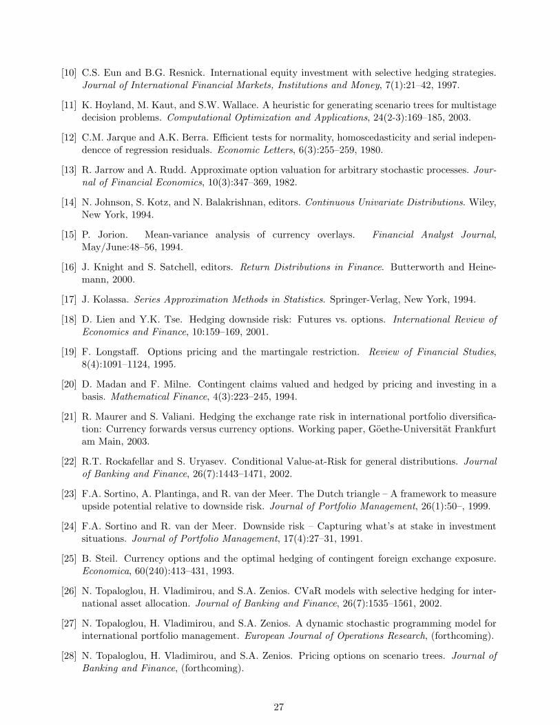
[10] C.S. Eun and B.G. Resnick. International equity investment with selective hedging strategies.Journal of International Financial Markets, Institutions and Money, 7(1):21–42, 1997.

[11] K. Hoyland, M. Kaut, and S.W. Wallace. A heuristic for generating scenario trees for multistagedecision problems. Computational Optimization and Applications, 24(2-3):169–185, 2003.

[12] C.M. Jarque and A.K. Berra. Efficient tests for normality, homoscedasticity and serial indepen-dencce of regression residuals. Economic Letters, 6(3):255–259, 1980.

[13] R. Jarrow and A. Rudd. Approximate option valuation for arbitrary stochastic processes. Jour-nal of Financial Economics, 10(3):347–369, 1982.

[14] N. Johnson, S. Kotz, and N. Balakrishnan, editors. Continuous Univariate Distributions. Wiley,New York, 1994.

[15] P. Jorion. Mean-variance analysis of currency overlays. Financial Analyst Journal,May/June:48–56, 1994.

[16] J. Knight and S. Satchell, editors. Return Distributions in Finance. Butterworth and Heine-mann, 2000.

[17] J. Kolassa. Series Approximation Methods in Statistics. Springer-Verlag, New York, 1994.

[18] D. Lien and Y.K. Tse. Hedging downside risk: Futures vs. options. International Review ofEconomics and Finance, 10:159–169, 2001.

[19] F. Longstaff. Options pricing and the martingale restriction. Review of Financial Studies,8(4):1091–1124, 1995.

[20] D. Madan and F. Milne. Contingent claims valued and hedged by pricing and investing in abasis. Mathematical Finance, 4(3):223–245, 1994.

[21] R. Maurer and S. Valiani. Hedging the exchange rate risk in international portfolio diversifica-tion: Currency forwards versus currency options. Working paper, Goethe-Universitat Frankfurtam Main, 2003.

[22] R.T. Rockafellar and S. Uryasev. Conditional Value-at-Risk for general distributions. Journalof Banking and Finance, 26(7):1443–1471, 2002.

[23] F.A. Sortino, A. Plantinga, and R. van der Meer. The Dutch triangle – A framework to measureupside potential relative to downside risk. Journal of Portfolio Management, 26(1):50–, 1999.

[24] F.A. Sortino and R. van der Meer. Downside risk – Capturing what’s at stake in investmentsituations. Journal of Portfolio Management, 17(4):27–31, 1991.

[25] B. Steil. Currency options and the optimal hedging of contingent foreign exchange exposure.Economica, 60(240):413–431, 1993.

[26] N. Topaloglou, H. Vladimirou, and S.A. Zenios. CVaR models with selective hedging for inter-national asset allocation. Journal of Banking and Finance, 26(7):1535–1561, 2002.

[27] N. Topaloglou, H. Vladimirou, and S.A. Zenios. A dynamic stochastic programming model forinternational portfolio management. European Journal of Operations Research, (forthcoming).

[28] N. Topaloglou, H. Vladimirou, and S.A. Zenios. Pricing options on scenario trees. Journal ofBanking and Finance, (forthcoming).

27