Embed Size (px)
Citation preview

Copyright © by SIAM. Unauthorized reproduction of this article is prohibited.
SIAM J. CONTROL OPTIM. c© 2009 Society for Industrial and Applied MathematicsVol. 48, No. 1, pp. 162–186
CONTROLLABILITY OF MULTI-AGENT SYSTEMS FROM AGRAPH-THEORETIC PERSPECTIVE∗
AMIRREZA RAHMANI†, MENG JI‡ , MEHRAN MESBAHI† , AND MAGNUS EGERSTEDT‡
Abstract. In this work, we consider the controlled agreement problem for multi-agent net-works, where a collection of agents take on leader roles while the remaining agents execute local,consensus-like protocols. Our aim is to identify reflections of graph-theoretic notions on system-theoretic properties of such systems. In particular, we show how the symmetry structure of thenetwork, characterized in terms of its automorphism group, directly relates to the controllability ofthe corresponding multi-agent system. Moreover, we introduce network equitable partitions as ameans by which such controllability characterizations can be extended to the multileader setting.
Key words. multi-agent systems, networked systems, controllability, automorphism group,equitable partitions, agreement dynamics, algebraic graph theory
AMS subject classifications. 93B05, 05C50, 05C25, 34B45, 94C15
DOI. 10.1137/060674909
1. Introduction. A networked system is a collection of dynamic units that in-teract over an information exchange network for its operation. Such systems areubiquitous in diverse areas of science and engineering. Examples include physiolog-ical systems and gene networks [12]; large-scale energy systems; and multiple space,air, and land vehicles [1, 2, 20, 27, 37, 38]. There is an active research effort underwayin the control and dynamical systems community to study these systems and lay outa foundation for their analysis and synthesis [6, 7, 9, 26]. As a result, over the pastfew years, a distinct area of research at the intersection of systems theory and graphtheory has emerged. An important class of problems that lies at this intersectionpertains to the agreement or the consensus problem [4, 15, 28, 30, 39]. The agreementproblem concerns the development of processes by which a group of dynamic units,through local interactions, reach a common value of interest. As such, the agreementprotocol is essentially an unforced dynamical system whose trajectory is governed bythe interconnection geometry and the initial condition for each unit.
Our goal in this paper is to consider situations where network dynamics can beinfluenced by external signals and decisions. In particular, we postulate a case in-volving nodes in the network that do not abide by the agreement protocol; we referto these agents as leaders or anchors.1 The complement of the set of leaders in thenetwork will be referred to as followers (respectively, floating nodes). The presence ofthese leader nodes generally alters the system behavior. The main topic under con-sideration in this paper is network controllability when leaders are agents of control.The controllability issue in leader-follower multi-agent systems was introduced in [36]
∗Received by the editors October 30, 2006; accepted for publication (in revised form) April 8,2008; published electronically February 11, 2009. A preliminary version of this work was presentedat the 2006 American Control Conference.
http://www.siam.org/journals/sicon/48-1/67490.html†Department of Aeronautics and Astronautics, University of Washington, Seattle, WA 98195
([email protected], [email protected]). The first and third authors are sup-ported by the National Science Foundation under grant ECS-0501606.
‡School of Electrical and Computer Engineering, Georgia Institute of Technology, Atlanta, GA30332 ([email protected], [email protected]). The second and fourth authors are sup-ported by the U.S. Army Research Office through grant 99838.
1Depending on the context, we could equally consider them as the nonconformist agents.
162
Copyright © by SIAM. Unauthorized reproduction of this article is prohibited.
CONTROLLABILITY FROM A GRAPH-THEORETIC PERSPECTIVE 163
by Tanner, who provided necessary and sufficient conditions for system controllabilityin terms of the eigenvectors of the graph Laplacian; we also refer to the related workof Olfati-Saber and Shamma in the context of consensus filters [31]. Subsequently,graph-theoretic characterizations of controllability for leader-follower multi-agent sys-tems were examined by Ji, Muhammad, and Egerstedt [18] and Rahmani and Mesbahi[34]. In the present work, we further explore the ramifications of this graph-theoreticoutlook on multi-agent systems controllability. First, we examine the roles of thegraph Laplacian eigenvectors and the graph automorphism group for single-leadernetworks. We then extend these results to multileader setting via equitable partitionsof the underlying graph.
This paper begins with the general form of the agreement dynamics over graphs.Next, we introduce transformations that, given the location of the leader nodes, pro-duce the corresponding controlled linear time-invariant system. The study of thecontrollability for single-leader systems is then pursued via tools from algebraic graphtheory. In this venue, we provide a sufficient graphical condition in terms of graphautomorphisms for the system’s uncontrollability. Furthermore, we introduce networkequitable partitions as a means by which such controllability characterizations can beextended to the multileader setting.
2. Notation and preliminaries. In this section we recall some basic notionsfrom graph theory, which is followed by the general setup of the agreement problemfor multi-agent networks.
2.1. Graphs and their algebraic representation. Graphs are broadly adopt-ed in the multi-agent literature to encode interactions in networked systems. Anundirected graph G is defined by a set VG = {1, . . . , n} of nodes and a set EG ⊂ VG×VGof edges. Two nodes i and j are neighbors if (i, j) ∈ EG ; the neighboring relation isindicated with i ∼ j, while P(i) = {j ∈ VG : j ∼ i} collects all neighbors of node i.The degree of a node is given by the number of its neighbors; we say that a graphis regular if all nodes have the same degree. A path i0i1 . . . iL is a finite sequenceof nodes such that ik−1 ∼ ik, k = 1, . . . , L, and a graph G is connected if there is apath between any pair of distinct nodes. A subgraph G′ is said to be induced fromthe original graph G if it can be obtained by deleting a subset of nodes and edgesconnecting to those nodes from G.
The adjacency matrix of the graph G, A(G) ∈ Rn×n, with n denoting the number
of nodes in the network, is defined by
[A(G) ]ij :={
1 if (i, j) ∈ EG ,0 otherwise.
If G hasm edges and is given an arbitrarily orientation, its node-edge incidence matrixB(G) ∈ R
n×m is defined as
[B(G) ]kl :=
⎧⎨⎩
1 if node k is the head of edge l,−1 if node k is the tail of edge l,0 otherwise,
where k and l are the indices running over the node and edge sets, respectively.A matrix that plays a central role in many graph-theoretic treatments of multi-
agent systems is the graph Laplacian, defined by
(1) L(G) := B(G)B(G)T ;
Copyright © by SIAM. Unauthorized reproduction of this article is prohibited.
164 A. RAHMANI, M. JI, M. MESBAHI, AND M. EGERSTEDT
thus the graph Laplacian is a (symmetric) positive semidefinite matrix. Let di be thedegree of node i, and let D(G) := Diag([di]ni=1) be the corresponding diagonal degreematrix. It is easy to verify that L(G) = D(G)−A(G) [11]. As the Laplacian is positivesemidefinite, its spectrum can be ordered as
0 = λ1(L(G)) ≤ λ2(L(G)) ≤ · · · ≤ λn(L(G)),
with λi(L(G)) being the ith ordered eigenvalue of L(G). It turns out that the multiplic-ity of the zero eigenvalue of the graph Laplacian is equal to the number of connectedcomponents of the graph [14]. In fact the second smallest eigenvalue λ2(L(G)) providesa judicious measure of the connectivity of G. For more on the related matrix-theoreticand algebraic approaches to graph theory, we refer the reader to [5, 14, 24].
2.2. Agreement dynamics. Given a multi-agent system with n agents, we canmodel the network by a graph G where nodes represent agents and edges are inter-agent information exchange links.2 Let xi(t) ∈ R
d denote the state of node i at timet, whose dynamics is described by the single integrator
xi(t) = ui(t), i = 1, . . . , n,
with ui(t) being node i’s control input. Next, we allow agent i to have access tothe relative state information with respect to its neighbors and use it to compute itscontrol. Hence, interagent coupling is realized through ui(t). For example, one canlet
(2) ui(t) = −∑i∼j
(xi(t) − xj(t)).
The localized rule in (2) happens to lead to the solution of the rendezvous problem,which has attracted considerable attention in the literature [8, 17, 22]. Some otherimportant networked system problems, e.g., formation control [3, 10, 13], consensusor agreement [25, 29, 30], and flocking [32, 35], share the same distributive flavor asthe rendezvous problem.
The single integrator dynamics in conjunction with (2) can be represented as theLaplacian dynamics of the form
x(t) = −L(G)x(t),(3)
where x(t) = [x(t)T1 , x(t)T2 , . . . , x(t)Tn ]T denotes the aggregated state vector of themulti-agent system, L(G) := L(G) ⊗ Id, with Id denoting the d-dimensional identitymatrix, and ⊗ is the matrix Kronecker product [16]. In fact, if the dynamics ofthe agent’s state is decoupled along each dimension, the behavior of the multi-agentsystem can be investigated one dimension at a time. Although our results can directlybe extended to the case of (3), in what follows we will focus on the system
x(t) = −L(G)x(t),(4)
capturing the multi-agent dynamics with individual agent states evolving in R.
2Throughout this paper we assume that the network is static. As such, the movements of theagents will not cause edges to appear or disappear in the network.
Copyright © by SIAM. Unauthorized reproduction of this article is prohibited.
CONTROLLABILITY FROM A GRAPH-THEORETIC PERSPECTIVE 165
1 2
3 4
65
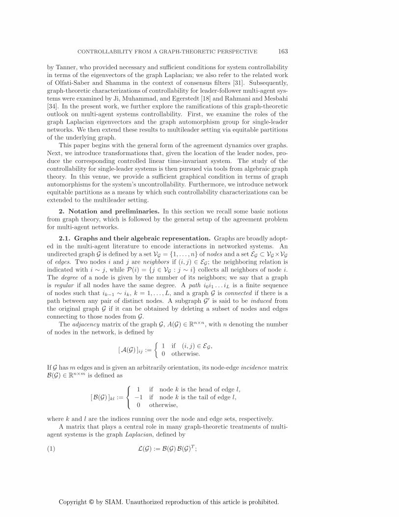
Fig. 1. A leader-follower network with Vf = {1, 2, 3, 4} and Vl = {5, 6}.
3. Controlled agreement. We now endow leadership roles to a subset of agentsin the Laplacian dynamics (4); the other agents in the network, the followers, continueto abide by the agreement protocol. In this paper, we use subscripts l and f to denoteaffiliations with leaders and followers, respectively. For example, a follower graph Gfis the subgraph induced by the follower node set Vf ⊂ VG . Leadership designationsinduce a partition of incidence matrix B(G) as
(5) B(G) =[ Bf (G)
Bl(G)
],
where Bf(G) ∈ Rnf×m, and Bl(G) ∈ R
nl×m. Here nf and nl are the cardinalities ofthe follower group and the leader group, respectively, and m is the number of edges.The underlying assumption of this partition, without loss of generality, is that leadersare indexed last in the original graph G. As a result of (1) and (5), the graph LaplacianL(G) is given by
(6) L(G) =[ Lf (G) lfl(G)lfl(G)T Ll(G)
],
where
Lf (G) = BfBTf , Ll(G) = BlBTl , and lfl(G) = BfBTl .Here we omitted the dependency of B,Bf , and Bl on G, which we will continue to dowhenever this dependency is clear from the context. As an example, Figure 1 showsa leader-follower network with Vl = {5, 6} and Vf = {1, 2, 3, 4}. This gives
Bf =
⎡⎢⎢⎣
1 0 0 −1 0 1 0 0−1 1 0 0 0 0 0 −1
0 −1 1 0 0 0 1 00 0 −1 1 −1 0 0 0
⎤⎥⎥⎦ , Bl=
[0 0 0 0 1 −1 0 00 0 0 0 0 0 −1 1
],
and
Lf (G) =
⎡⎢⎢⎣
3 −1 0 −1−1 3 −1 0
0 −1 3 −1−1 0 −1 3
⎤⎥⎥⎦ , lfl(G) =
⎡⎢⎢⎣
−1 00 −10 −1
−1 0
⎤⎥⎥⎦ .
The control system we now consider is the controlled agreement dynamics (orleader-follower system), where followers evolve through the Laplacian-based dynamics
xf (t) = −Lf xf (t) − lfl u(t),(7)

Copyright © by SIAM. Unauthorized reproduction of this article is prohibited.
166 A. RAHMANI, M. JI, M. MESBAHI, AND M. EGERSTEDT
where u denotes the exogenous control signal dictated by the leaders’ states.Definition 3.1. Let l be a leader node in G, i.e., l ∈ Vl(G). The indicator vector
with respect to l,
δl : Vf → {0, 1}nf ,
is such that
δl(i) :={
1 if i ∼ l,0 otherwise.
We note that each column of −lfl is an indicator vector, i.e., lfl = [−δnf+1, . . . ,−δn].Let dil, with i ∈ Vf , denote the number of leaders adjacent to follower i, and
define the follower-leader degree matrix
(8) Dfl(G) := Diag([dil]nf
i=1),
which leads to the relationship
(9) Lf (G) = L(Gf ) + Dfl(G),
where L(Gf ) is the Laplacian matrix of the follower graph Gf .Remark 3.2. We should emphasize the difference between Lf (G) and L(Gf ). The
matrix Lf (G) is the principle diagonal submatrix of the original Laplacian matrixL(G) related to the followers, while L(Gf ) is the Laplacian matrix of the subgraph Gfinduced by the followers. For simplicity, we will write Lf and lfl to represent Lf (G)and lfl(G), respectively, when their dependency on G is clear from the context.
Since the row sum of the Laplacian matrix is zero, the sum of the ith row ofLf (G) and that of −lfl(G) are both equal to dil, i.e.,
(10) Lf (G)1nf= Dfl(G)1nf
= −lfl(G)1nl,
where 1 is a vector with ones at each component.If there is only one leader in the network, then according to the indexing con-
vention, Vl = {n}. In this case, we have lfl(G) = −δn and Dfl(G) = Diag(δn). Forinstance, the indicator vector for the node set Vf = {1, 2, 3} in the graph shown inFigure 2 with respect to the leader {4} is δ4 = [ 1, 1, 0 ]T .
Proposition 3.3. If a single node is chosen to be the leader, the original Lapla-cian L(G) is related to the Laplacian of the follower graph L(Gf ) via
L(G) =[ L(Gf ) + Dfl(G) −δn
−δTn dn
],(11)
where dn denotes the degree of agent n.
Fig. 2. Path graph with node “4” being the leader.
Another way to construct the system matrices Lf (G) and lfl(G) is from the Lapla-cian of the original graph via
Lf = PTf L(G)Pf and lfl = PTf L(G)Tfl,(12)

Copyright © by SIAM. Unauthorized reproduction of this article is prohibited.
CONTROLLABILITY FROM A GRAPH-THEORETIC PERSPECTIVE 167
where Pf ∈ Rn×nf is constructed by eliminating the columns of the n × n identity
matrix that correspond to the leaders, and Tfl ∈ Rn×nl is formed by grouping these
eliminated columns into a new matrix. For example, in Figure 1 these matrices assumethe form
Pf =[
I402×4
]and Tfl =
[04×2
I2
].
Proposition 3.4. If a single node is chosen to be the leader, one has
Tfl = (In − P )1n and lfl = −Lf1nf
in (12), where P = [Pf 0n×nl] is the n× n square matrix obtained by expanding Pf
with zero block of proper dimensions.Proof. The first equality directly follows from the definition of Pf and Tfl. With-
out loss of generality, assume that the last node is the leader; then [Pf Tfl ] = In.Multiplying both sides by 1n and noting that P 1n = Pf1nf
, one has Tfl = (In−P )1n.Moreover,
lfl = PTf L(G){(I − P )1n} = PTf L(G)1n − PTf L(G)Pf1nf.
The first term on the right-hand side of the equality is zero, as 1 belongs to the nullspace of L(G); the second term, on the other hand, is simply Lf1.
Alternatively, for the case when the exogenous signal is constant, the dynamics(7) can be rewritten as[
xf (t)u(t)
]= −
[ Lf lfl0 0
] [xf (t)u(t)
].(13)
This corresponds to zeroing-out the rows of the original graph Laplacian associatedwith the leader. Zeroing-out a row of a matrix can be accomplished via a reducedidentity matrix Qr, with zeros at the diagonal elements that correspond to the leaders,with all other diagonal elements being kept as one. In this case,[ Lf lfl
0 0
]= QrL(G),(14)
where
Qr =[Inf
00 0
],
and all the zero matrices are of proper dimensions.
4. Reachability. First, we examine whether we can steer the system (7) intothe agreement subspace, span{1}, when the exogenous signal is constant, i.e., xi = c,for all i ∈ Vl and c ∈ R is a constant. As shown in (14), in this case the controlledagreement can be represented as
x(t) = −QrL(G)x(t) = −Lr(G)x(t),(15)
where Qr is the reduced identity matrix and Lr(G) := QrL(G) is the reduced Lapla-cian matrix. Let us now examine the convergence properties of (15) with respect to
Copyright © by SIAM. Unauthorized reproduction of this article is prohibited.
168 A. RAHMANI, M. JI, M. MESBAHI, AND M. EGERSTEDT
span{1}. Define ζ(t) as the projection of the followers’ state xf (t) onto the sub-space orthogonal to the agreement subspace span{1}. This subspace is denoted by1⊥; in [30] it is referred to as the disagreement subspace. One can then model thedisagreement dynamics as
ζ(t) = −Lr(G) ζ(t).(16)
Choosing a standard quadratic Lyapunov function for (16),
V (ζ(t)) =12ζ(t)T ζ(t),
reveals that its time rate of change assumes the form
V (ζ(t)) = −ζ(t)T Lr(G) ζ(t),
where Lr(G) = (1/2) [Lr(G) + Lr(G)T ].Proposition 4.1. The agreement subspace is reachable for the controlled agree-
ment protocol (7).Proof. Since V (ζ) < 0 for all ζ �= 0 and QrL(G)1 = 0, for any leader nodes, the
agreement subspace remains a globally attractive subspace of (15).Proposition 4.2. In the case of one leader, the matrix Lr(G) has a real spectrum
and the same inertia as L(G).Proof. Let E = 11T denote the matrix of all ones. Since EL(G) = 0 and
QrL(G) = Lr(G), (Qr + E)L(G) = Lr(G). Hence Lr(G) is a product of a positivedefinite matrix, namely Qr+E, and the symmetric matrix L(G). By Theorem 7.6.3 of[16], Lr(G) is diagonalizable and has a real spectrum. In fact, it has the same inertiaas L(G).
5. Controllability analysis of single-leader networks. In this section, weinvestigate the controllability properties of single-leader networks. Following our pre-viously mentioned indexing convention, the index of the leader is assumed to be n.For notational convenience in this section, we will equate xf with x and xl with u.Moreover, we identify matrices A and B with −Lf and −lfl, respectively. Thus, thesystem (7) is specified by
(17) x(t) = Ax(t) +Bu(t).
The controllability of the controlled agreement (17) can be investigated using thePopov–Hautus–Belevitch (PHB) test [19, 33]. Specifically, (17) is uncontrollable ifand only if there exists a left eigenvector ν of A, i.e., νTA = λνT for some λ, suchthat
νTB = 0.
Since A is symmetric, its left and right eigenvectors are the same. Hence, the necessaryand sufficient condition for controllability of (17) is that none of the eigenvectors ofA should be simultaneously orthogonal to all columns of B. Additionally, in order toinvestigate the controllability of (17), one can form the controllability matrix as
C = [B AB · · · Anf−1B ].(18)
As A is symmetric, it can be written in the form UΛUT , where Λ is the diagonalmatrix of eigenvalues of A; U , on the other hand, is the unitary matrix comprised of
Copyright © by SIAM. Unauthorized reproduction of this article is prohibited.
CONTROLLABILITY FROM A GRAPH-THEORETIC PERSPECTIVE 169
A’s pairwise orthogonal unit eigenvectors. Since B = UUTB, by factoring the matrixU from the left in (18), the controllability matrix assumes the form
C = U [UTB ΛUTB . . . Λnf−1UTB ].(19)
In this case, U is full rank and its presence does not alter the rank of the matrixproduct in (19). If one of the columns of U is perpendicular to all the columns of B,then C will have a row equal to zero, and hence the matrix C is rank deficient [36].On the other hand, in the case of one leader, if any two eigenvalues of A are equal,then C will have two linear dependent rows, and again, the controllability matrixbecomes rank deficient. Assume that ν1 and ν2 are two eigenvectors correspondingto the same eigenvalue and that none of them is orthogonal to B. Then ν = ν1 + cν2is also an eigenvector of A for that eigenvalue. This will then allow us to choosec = −νT1 B/νT2 B, which renders νTB = 0. In other words, we are able to find aneigenvector that is orthogonal to B. Hence, we arrive at the following observation.
Proposition 5.1. Consider a leader-follower network whose evolution is de-scribed by (17). This system is controllable if and only if none of the eigenvectors ofA is (simultaneously) orthogonal to (all columns of) B. Moreover, if A does not havedistinct eigenvalues, then (17) is not controllable.
Proposition 5.1 is also valid for the case with more than one leader and impliesthat in any finite time interval, the floating dynamic units can be independentlysteered from their initial states to an arbitrary final one based on local interactionswith their neighbors. This controllability results is of course valid when the states ofthe leader nodes are assumed to be unconstrained.
Corollary 5.2. The networked system (17) with a single leader is controllableif and only if none of the eigenvectors of A is orthogonal to 1.
Proof. As shown in Proposition 3.4, the elements of B correspond to row-sums ofA, i.e., B = −A1. Thus, νTB = −νTA1 = −λ (νT 1). By Proposition 4.2 one hasλ �= 0. Thereby, νTB = 0 if and only if 1T ν = 0.
Proposition 5.3. If the networked system (17) is uncontrollable, there exists aneigenvector ν of A such that
∑i∼n ν(i) = 0.
Proof. Using Corollary 5.2, when the system is uncontrollable, there exists aneigenvector of A that is orthogonal to 1. As Aν = λν, we deduce that 1T (Aν ) = 0.Moreover, using Proposition 3.3, we obtain
νT {L(Gf ) + Dfl(G) } 1 = 0.
But L(Gf )1 = 0, and thereby
νT Dfl(G)1 = νT δn = 0,
which implies that∑
i∼n ν(i) = 0.Proposition 5.4. Suppose that the leader-follower system (17) is uncontrollable.
Then there exists an eigenvector of L(G) that has a zero component on the index thatcorresponds to the leader.
Proof. Let ν be an eigenvector of A that is orthogonal to 1 (by Corollary 5.2,such an eigenvector exists). Attach a zero to ν; using the partitioning (11), we thenhave
L(G)[ν0
]=
[A −δn
−δTn dn
] [ν0
]=
[λν
−δTn ν],
Copyright © by SIAM. Unauthorized reproduction of this article is prohibited.
170 A. RAHMANI, M. JI, M. MESBAHI, AND M. EGERSTEDT
where δn is the indicator vector of the leader’s neighbors. From Proposition 5.3 weknow that δTn ν = 0. Thus,
L(G)[ν0
]= λ
[ν0
].
In the other words, L(G) has an eigenvector with a zero on the index that correspondsto the leader.
A direct consequence of Proposition 5.4 is the following.Corollary 5.5. Suppose that none of the eigenvectors of L(G) has a zero compo-
nent. Then the leader-follower system (7) is controllable for any choice of the leader.
5.1. Controllability and graph symmetry. The controllability of the inter-connected system depends not only on the geometry of the interunit informationexchange but also on the position of the leader with respect to the graph topology. Inthis section, we examine the controllability of the system in terms of graph-theoreticproperties of the network. In particular, we will show that there is an intricate re-lation between the controllability of (17) and the symmetry structure of the graph,as captured by its automorphism group. We first need to introduce a few usefulconstructs.
Definition 5.6. A permutation matrix is a {0, 1}-matrix with a single nonzeroelement in each row and column.
Definition 5.7. The system (17) is anchor symmetric with respect to anchor aif there exists a nonidentity permutation J such that
JA = AJ,(20)
where A = −Lf = −PTf L(G)Pf is constructed as in (12). We call the system asym-metric if it does not admit such a permutation for any anchor.
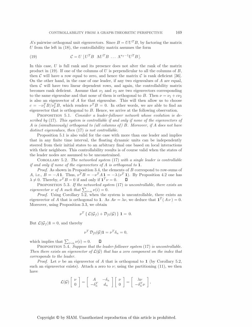
As an example, the graph represented in Figure 3(a) is leader symmetric withrespect to {6} but asymmetric with respect to any other leader node set. On theother hand, the graph of Figure 3(b) is leader symmetric with respect to a singleleader located at every node. The utility of the notion of leader symmetry is nowestablished through its relevance to the system-theoretic concept of controllability.
Fig. 3. Interconnected topologies that are leader symmetric: (a) only with respect to node {6};(b) with respect to a leader at any node.
Proposition 5.8. The system (17) is uncontrollable if it is leader symmetric.Proof. If the system is leader symmetric, then there is a nonidentity permutation
J such that
JA = AJ.(21)
Recall that, by Proposition 5.1, if the eigenvalues of A are not distinct, then (17) is notcontrollable. We thus consider the case where all eigenvalues λ are distinct and satisfy
Copyright © by SIAM. Unauthorized reproduction of this article is prohibited.
CONTROLLABILITY FROM A GRAPH-THEORETIC PERSPECTIVE 171
Aν = λν; thereby, for all eigenvalue/eigenvector pairs (λ, ν) one has JAν = J(λν).Using (21), however, we see that A (Jν) = λ (Jν), and Jν is also an eigenvector ofA corresponding to the eigenvalue λ. Given that λ is distinct and A admits a set oforthonormal eigenvectors, we conclude that for one such eigenvector ν, ν − Jν is alsoan eigenvector of A. Moreover, J B = JTB = B, as the elements of B correspond tothe row-sums of the matrix A, i.e., B = −A1. Thereby,
(ν − Jν)TB = νTB − νTJT B = νTB − νTB = 0.(22)
This, on the other hand, translates into having one of the eigenvectors of A, namelyν − Jν, be orthogonal to B. Proposition 5.1 now implies that the system (17) isuncontrollable.
Proposition 5.8 states that leader symmetry is a sufficient condition for uncon-trollability of the system. It is instructive to examine whether leader asymmetry leadsto a controllable system.
Proposition 5.9. Leader symmetry is not a necessary condition for systemuncontrollability.
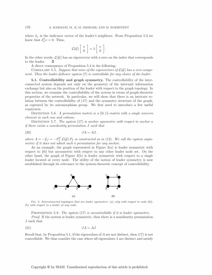
Proof. In Figure 4, the subgraph shown by solid lines, Gf , is the smallest asym-metric graph [21], in the sense that it does not admit any nonidentity automorphism.Let us augment this graph with the node “a” and connect it to all vertices of Gf .Constructing the corresponding system matrix A (i.e., setting it equal to −Lf (G)),we have
−A = L(Gf ) + Dfl(G) = L(Gf ) + I,
where I is the identity matrix of proper dimensions. Consequently, A has the sameset of eigenvectors as L(Gf ). Since L(Gf ) has an eigenvector orthogonal to 1, A alsohas an eigenvector that is orthogonal to 1. Hence, the leader-follower system is notcontrollable. Yet, the system is not symmetric with respect to a; more on this willappear in section 5.2.
Fig. 4. Asymmetric information topology with respect to the leader {a}. The subgraph shownby solid lines is the smallest asymmetric graph.
It is intuitive that a highly connected leader will result in faster convergenceto the agreement subspace. However, a highly connected leader also increases thechances that a symmetric graph, with respect to leader, emerges. A limiting casefor this latter scenario is the complete graph. In such a graph, n − 1 leaders areneeded to make the corresponding controlled system controllable. This requirementis of course not generally desirable, as it means that the leader group includes allnodes except for one node! The complete graph is “the worse” case configuration asfar as its controllability properties. Generally at most n − 1 leaders are needed tomake any information exchange network controllable. In the meantime, a path graph

Copyright © by SIAM. Unauthorized reproduction of this article is prohibited.
172 A. RAHMANI, M. JI, M. MESBAHI, AND M. EGERSTEDT
with a leader at one end is controllable. Thus it is possible to make a complete graphcontrollable by keeping the links on the longest path between a leader and all othernodes and deleting the unnecessary information exchange links to break its inherentsymmetry. This procedure is not always feasible; for example, a star graph is notamenable to such graphical alterations.
5.2. Leader symmetry and graph automorphism. In section 5.1 we dis-cussed the relationship between leader symmetry and controllability. In this sectionwe will further explore the notion of leader symmetry with respect to graph automor-phisms.
Definition 5.10. An automorphism of G = (V , E) is a permutation ψ of its nodeset such that
(ψ(i) , ψ(j)) ∈ EG ⇐⇒ (i, j) ∈ EG .
The set of all automorphisms of G, equipped with the composition operator,constitutes the automorphism group of G; note that this is a “finite” group. It is clearthat the degree of a node remains unchanged under the action of the automorphismgroup; i.e., if ψ is an automorphism of G, then dv = dψ(v) for all v ∈ VG .
Proposition 5.11 (see [5]). Let A(G) be the adjacency matrix of the graph G andψ a permutation on its node set V. Associate with this permutation the permutationmatrix Ψ such that
Ψij :={
1 if ψ(i) = j,0 otherwise.
Then ψ is an automorphism of G if and only if
ΨA(G) = A(G)Ψ.
In this case, the least positive integer z for which Ψz = I is called the order of theautomorphism.
Recall that from Definition 5.7 leader symmetry for (17) corresponds to having
JA = AJ,
where J is a nonidentity permutation. From Proposition 3.3, however,
A = −(L(Gf ) + Dfl(G)).
Thus using the identity L(Gf ) = D(Gf ) −A(Gf ), one has
J {D(Gf ) −A(Gf ) + Dfl(G)} = {D(Gf ) −A(Gf ) + Dfl(G)} J.(23)
Pre- and postmultiplication of (a permutation matrix) J does not change the structureof diagonal matrices. Also, all diagonal elements of A(G) are zero. We can therebyrewrite (23) as two separate conditions,
JDf (G) = Df (G)J and JA(Gf ) = A(Gf )J,(24)
with Df (G) := D(Gf ) + Dfl(G). The second equality in (24) states that sought afterJ in (20) is in fact an automorphism of Gf .
Copyright © by SIAM. Unauthorized reproduction of this article is prohibited.
CONTROLLABILITY FROM A GRAPH-THEORETIC PERSPECTIVE 173
Proposition 5.12. Let Ψ be the permutation matrix associated with ψ. ThenΨDf(G) = Df (G)Ψ if and only if
di + δn(i) = dψ(i) + δn(ψ(i)).
In the case where ψ is an automorphism of Gf , this condition simplifies to
δn(i) = δn(ψ(i)).
Proof. Using the properties of permutation matrices, one has
[ΨDf(G)]ik =∑t
ΨitDtk ={dk + δn(k) if i→ k,
0 otherwise
and
[Df (G)Ψ]ik =∑t
Dit Ψtk ={di + δn(i) if i→ k,
0 otherwise.
For these matrices to be equal elementwise, one needs to have di + δn(i) = dk +δn(k) when ψ(i) = k. The second statement in the proposition follows from the factthat the degree of a node remains invariant under the action of the automorphismgroup.
The next two results follow immediately from the above discussion.Proposition 5.13. The interconnected system (17) is leader symmetric if and
only if there is a nonidentity automorphism for Gf such that the indicator functionremains invariant under its action.
Corollary 5.14. The interconnected system (17) is leader asymmetric if theautomorphism group of the floating (or follower) subgraph contains only the trivial(identity) permutation.
5.3. Controllability of special graphs. In this section we investigate the con-trollability of ring and path graphs.
Proposition 5.15. A ring graph, with only one leader, is never controllable.Proof. With only one leader in the ring graph, the follower graph Gf becomes
the path graph with one nontrivial automorphism, i.e., its mirror image. Withoutloss of generality, choose the first node as the leader and index the remaining followernodes by a clockwise traversing of the ring. Then the permutation i → n − i+ 2 fori = 2, . . . , n is an automorphism of Gf . In the meantime, the leader “1” is connectedto both node 2 and node n; hence δn = [ 1, 0, . . . , 0, 1 ]T remains invariant underthe permutation. Using Proposition 5.13, we conclude that the corresponding system(17) is leader symmetric and thus uncontrollable.
Proposition 5.16. A path graph is controllable for all choices of the leader nodeif and only if it is of even order.
Proof. Suppose that the path graph is of odd order; then choose the middle noden+1
2 as the leader. Note that ψ(k) = n − k + 1 is an automorphism for the floatingsubgraph. Moreover, the leader is connected to nodes n+1
2 − 1 and n+12 + 1, and
ψ(n+12 − 1) = n+1
2 + 1. Thus
δn = [ 0, . . . , 0, 1, 1, 0, . . . , 0 ]T
remains invariant under the permutation ψ and the system is uncontrollable. Theconverse statement follows analogously.
Copyright © by SIAM. Unauthorized reproduction of this article is prohibited.
174 A. RAHMANI, M. JI, M. MESBAHI, AND M. EGERSTEDT
Hence although in general leader symmetry is a sufficient—yet not necessary—condition for uncontrollability of (17), it is necessary and sufficient for uncontrollabil-ity of the path graph.
Corollary 5.17. A path graph with a single leader is controllable if and only ifit is leader asymmetric.
6. Rate of convergence. In previous sections, we discussed controllabilityproperties of controlled agreement dynamics in terms of the symmetry structure of thenetwork. When the resulting system is controllable, the nodes can reach agreementarbitrarily fast.
Proposition 6.1. A controllable agreement dynamics (17) can reach the agree-ment subspace arbitrarily fast.
Proof. The (invertible) controllability Grammian for (17) is defined as
Wa(t0, tf ) =∫ tf
t0
esABBT esAT
ds.(25)
For any tf > t0, the leader can then transmit the signal
u(t) = BT eAT (tf−t0)Wa(t0, tf )−1
(xf − eA(tf−t0)x0
)(26)
to its neighbors; in (26) x0 and xf are the initial and final states for the followernodes, and t0 and tf are prespecified initial and final maneuver times.
Next let us examine the convergence properties of the leader-follower networkwith a leader that transmits a constant signal (15). In this venue, define the quantity
μ2(Lr(G)) := minζ �=0ζ⊥1
ζT Lr(G) ζζT ζ
.(27)
Proposition 6.2. The rate of convergence of the disagreement dynamics (16) isbounded by μ2(Lr(G)) and λ2(L(G)), when the leader transmits a constant signal.
Proof. Using the variational characterization of the second smallest eigenvalue ofthe graph Laplacian [14, 16], we have
λ2(L(G)) = minζ �=0ζ⊥1
ζTL(G)ζζT ζ
≤ minζ �=0ζ⊥1
ζ=Qβ
ζTL(G)ζζT ζ
= minQβ �=0Qβ⊥1
βTQL(G)QββTQβ
= minQβ �=0Qβ⊥1
βTQ{
12 (QL(G) + L(G)Q)
}Qβ
βTQβ
= minQβ �=0Qβ⊥1
βTQ(
12 (Lr(G) + Lr(G)T )
)Qβ
βTQβ
= minζ �=0ζ⊥1
ζTLr(G)ζζT ζ
= μ2(Lr(G)),
where β is an arbitrary vector with the appropriate dimension, Q is the matrix in-troduced in (14), and Q2 = Q. In the last variational statement, we observe that ζ
Copyright © by SIAM. Unauthorized reproduction of this article is prohibited.
CONTROLLABILITY FROM A GRAPH-THEORETIC PERSPECTIVE 175
should have a special structure, i.e., ζ = Qβ (a zero at the row corresponding to theleader). An examination of the error dynamics suggests that such a structure alwaysexists. As the leader does not update its value in the static leader case, the differencebetween the leader’s state and the agreement value is always zero. Thus with respectto the disagreement dynamics (16),
V (ζ) = −ζT Lr(G) ζ ≤ −μ2(Lr(G))ζT ζ≤ −λ2(L(G)) ζT ζ.
7. Controllability of multiple-leader networks. Some applications of multi-agent systems may require multiple leaders. As our subsequent discussion shows, inthis case, one needs an additional set of graph-theoretic tools to analyze the networkcontrollability. In this venue, we first introduce equitable partitions and interlacingtheory that play important roles in our analysis. We then present the main theo-rem of this section, providing a graph-theoretic characterization of controllability formultiple-leader networks.
7.1. Interlacing and equitable partitions. A cell C ⊂ VG is a subset of thenode set. A partition of the graph is then a grouping of its node set into differentcells.
Definition 7.1. An r-partition π of VG, with cells C1, . . . , Cr, is said to beequitable if each node in Cj has the same number of neighbors in Ci for all i, j. Wedenote the cardinality of the partition π by r = |π|.
Let bij be the number of neighbors in Cj of a node in Ci. The directed graph withthe cells of an equitable r-partition π as its nodes, and with bij edges from the ith tothe jth cells of π, is called the quotient of G over π and is denoted by G/π. An obvioustrivial partition is the n-partition, π = {{1}, {2}, . . . , {n}}. If an equitable partitioncontains at least one cell with more than one node, we call it a nontrivial equitablepartition (NEP), and the adjacency matrix of a quotient is given by
A(G/π)ij = bij .
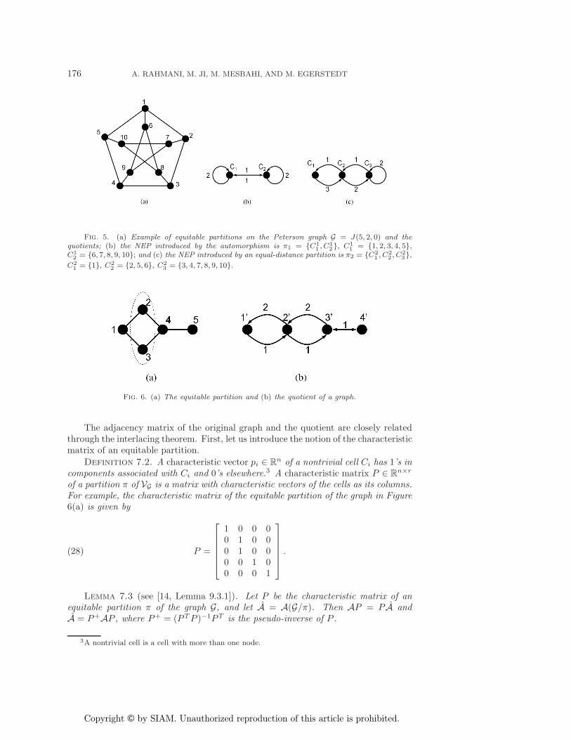
Equitable partitions of a graph can be obtained from its automorphisms. Forexample, in the Peterson graph shown in Figure 5(a), one equitable partition π1
(Figure 5(b)) is given by the two orbit of the automorphism groups, namely the 5inner vertices and the 5 outer vertices. The adjacency matrix of the quotient is thengiven by
A(G/π1) =[
2 11 2
].
The equitable partition can also be introduced by the equal distance partition.Let C1 ⊂ VG be a given cell, and let Ci ⊂ VG be the set of vertices at distance i− 1from C1. C1 is said to be completely regular if its distance partition is equitable. Forinstance, every node in the Peterson graph is completely regular and introduces thepartition π2 as shown in Figure 5(c). The adjacency matrix of this quotient is givenby
A(G/π2) =
⎡⎣ 0 3 0
1 0 20 1 2
⎤⎦ .
Copyright © by SIAM. Unauthorized reproduction of this article is prohibited.
176 A. RAHMANI, M. JI, M. MESBAHI, AND M. EGERSTEDT
Fig. 5. (a) Example of equitable partitions on the Peterson graph G = J(5, 2, 0) and thequotients; (b) the NEP introduced by the automorphism is π1 = {C1
1 , C12}, C1
1 = {1, 2, 3, 4, 5},C1
2 = {6, 7, 8, 9, 10}; and (c) the NEP introduced by an equal-distance partition is π2 = {C21 , C2
2 , C23},
C21 = {1}, C2
2 = {2, 5, 6}, C23 = {3, 4, 7, 8, 9, 10}.
Fig. 6. (a) The equitable partition and (b) the quotient of a graph.
The adjacency matrix of the original graph and the quotient are closely relatedthrough the interlacing theorem. First, let us introduce the notion of the characteristicmatrix of an equitable partition.
Definition 7.2. A characteristic vector pi ∈ Rn of a nontrivial cell Ci has 1’s in
components associated with Ci and 0’s elsewhere.3 A characteristic matrix P ∈ Rn×r
of a partition π of VG is a matrix with characteristic vectors of the cells as its columns.For example, the characteristic matrix of the equitable partition of the graph in Figure6(a) is given by
(28) P =
⎡⎢⎢⎢⎢⎣
1 0 0 00 1 0 00 1 0 00 0 1 00 0 0 1
⎤⎥⎥⎥⎥⎦ .
Lemma 7.3 (see [14, Lemma 9.3.1]). Let P be the characteristic matrix of anequitable partition π of the graph G, and let A = A(G/π). Then AP = P A andA = P+AP , where P+ = (PTP )−1PT is the pseudo-inverse of P .
3A nontrivial cell is a cell with more than one node.
Copyright © by SIAM. Unauthorized reproduction of this article is prohibited.
CONTROLLABILITY FROM A GRAPH-THEORETIC PERSPECTIVE 177
As an example, the graph in Figure 6 has a nontrivial cell (2, 3). The adjacencymatrix of the original graph is
A =
⎡⎢⎢⎢⎢⎣
0 1 1 0 01 0 0 1 01 0 0 1 00 1 1 0 10 0 0 1 0
⎤⎥⎥⎥⎥⎦ .
The adjacency matrix of the quotient, on the other hand, is
A = P+AP =
⎡⎢⎢⎣
0 2 0 01 0 1 00 2 0 10 0 1 0
⎤⎥⎥⎦ .
Lemma 7.4 (see [14, Lemma 9.3.2]). Let G be a graph with adjacency matrix A,and let π be a partition of VG with characteristic matrix P . Then π is equitable if andonly if the column space of P is A-invariant.
Lemma 7.5 (see [23]). Given a symmetric matrix A ∈ Rn×n, let S be a subspace
of Rn. Then S⊥ is A-invariant if and only if S is A-invariant.The proof of this lemma is well known and can be found, for example, in [23].Remark 7.6. Let R(·) denote the range space. Suppose |VG | = n, |Ci| = ni, and
|π| = r. Then we can find an orthogonal decomposition of Rn as
(29) Rn = R(P ) ⊕R(Q).
In this case the matrix Q satisfies R(Q) = R(P )⊥, and its columns, together withthose of P , form a basis for R
n. Note that by Lemma 7.5, R(Q) is also A-invariant.One way of obtaining the Q matrix is via the orthonormal basis of R(P )⊥. Let
us denote the normalized matrix (each column of which is a norm one vector) by Q.Next, define
(30) P = P (PTP )−12
as the normalized P matrix.4 Since P and Q have the same column space as P andQ, respectively, they satisfy PT Q = 0 and QT Q = In−r. In other words,
(31) T = [P | Q]
is a matrix, constructed based on the equitable partition π, whose columns constitutean orthonormal basis for R
n.Theorem 7.7 (see [14, Theorem 9.3.3]). If π is an equitable partition of a
graph G, then the characteristic polynomial of A = A(G/π) divides the characteristicpolynomial of A(G).
Lemma 7.8 (see [14, Theorem 9.5.1]). Let Φ ∈ Rn×n be a real symmetric matrix,
and let R ∈ Rn×m be such that RTR = Im. Set Θ = RTΦR and let ν1, ν2, . . . , νm be
an orthogonal set of eigenvectors for Θ such that Θνi = λi(Θ)νi, where λi(Θ) ∈ R is
4Note that the invertibility of P T P follows from the fact that the cells of the partition arenonempty. In fact, P T P is a diagonal matrix with (P T P )ii = |Ci|.
Copyright © by SIAM. Unauthorized reproduction of this article is prohibited.
178 A. RAHMANI, M. JI, M. MESBAHI, AND M. EGERSTEDT
an eigenvalue of Θ. Then1. the eigenvalues of Θ interlace the eigenvalues of Φ.2. if λi(Θ) = λi(Φ), then there is an eigenvector v of Θ with eigenvalue λi(Θ)
such that Rν is an eigenvector of Φ with eigenvalue λi(Φ).3. if λi(Θ) = λi(Φ) for i = 1, . . . , l, then Rνi is an eigenvector for Φ with
eigenvalue λi(Φ) for i = 1, . . . , l.4. if the interlacing is tight, then ΦR = RΘ.
Based on the controllability results introduced in section 5, together with somebasic properties of the graph Laplacian, we first derive the following lemma.
Lemma 7.9. Given a connected graph, the system (7) is controllable if and onlyif L and Lf do not share any common eigenvalues.
Proof. We can reformulate the lemma as stating that the system is uncontrollableif and only if there exists at least one common eigenvalue between L and Lf .
Necessity. Suppose that the system is uncontrollable. Then by Proposition 5.1there exists a vector νi ∈ R
nf such that Lfνi = λνi for some λ ∈ R, with lTflνi = 0.Now, since
[ Lf lfllTfl Ll
] [νi0
]=
[ LfνilTflνi
]= λ
[νi0
],
λ is also an eigenvalue of L, with eigenvector [νTi ,0]T . The necessary condition thusfollows.
Sufficiency. It suffices to show that if L and Lf share a common eigenvalue, thenthe system (L, lfl) is not completely controllable. Since Lf is a principal submatrixof L, it can be given by
Lf = PTf LPf ,
where Pf = [Inf, 0]T is the n × nf matrix defined in (12). Following the fourth
statement of Lemma 7.8,5 if Lf and L share a common eigenvalue, say λ, then thecorresponding eigenvector satisfies
ν = Pfνf =[νf0
],
where ν is λ’s eigenvector of L and νf is that of Lf . Moreover, we know that
Lν =[ Lf lfllTfl Ll
] [νf0
]= λ
[νf0
],
which gives us lTflνf = 0; thus the system is uncontrollable.Remark 7.10. Lemma 7.9 is an extension of Corollary 5.2, Propositions 5.3, and
Proposition 5.4 to multileader settings.
7.2. Controllability analysis based on equitable partitions. In this sec-tion, we will utilize a graph-theoretic approach to characterize the necessary conditionfor a multiple-leader networked system to be controllable. The way we approach thisnecessary condition is through Lemma 7.9. In what follows we will show first thatmatrices L and Lf are both similar to some block diagonal matrices. Furthermore,
5Here the matrix Pf plays the same role as the matrix R in the fourth statement of Lemma 7.8.

Copyright © by SIAM. Unauthorized reproduction of this article is prohibited.
CONTROLLABILITY FROM A GRAPH-THEORETIC PERSPECTIVE 179
we show that under certain assumptions, the diagonal block matrices obtained fromthe diagonalization of L and Lf have common diagonal block(s).
Lemma 7.11. If a graph G has an NEP π with characteristic matrix P , then thecorresponding adjacency matrix A(G) is similar to a block diagonal matrix
A =[ AP 0
0 AQ
],
where AP is similar to the adjacency matrix A = A(G/π) of the quotient graph.Proof. Let the matrix T = [P | Q] be the orthonormal matrix with respect to π,
as defined in (31). Let
(32) A = T TAT =[PTAP PTAQQTAP QTAQ
].
Since P and Q have the same column spaces as P and Q, respectively, they inherittheir A-invariance property, i.e., there exist matrices B and C such that
AP = PB and AQ = QC.
Moreover, since the column spaces of P and Q are orthogonal complements of eachother, one has
PTAQ = PT QC = 0
and
QTAP = QT PB = 0.
In addition, by letting D2p = PTP , we obtain
(33) PTAP = D−1P PTAPD−1
P = DP (D−2P PTAP )D−1
P = DP AD−1P ,
and therefore the first diagonal block is similar to A.Lemma 7.12. Let P be the characteristic matrix of an NEP in G. Then R(P ) is
K-invariant, where K is any diagonal block matrix of the form
K = Diag([k1, . . . , k1︸ ︷︷ ︸n1
, k2, . . . , k2︸ ︷︷ ︸n2
, . . . , kr, . . . , kr︸ ︷︷ ︸nr
]T ) = Diag([ki1ni ]ri=1),
ki ∈ R, ni = |Ci| is the cardinality of the cell, and r = |π| is the cardinality of thepartition. Consequently,
QTKP = 0,
where P = P (PTP )−12 and Q is chosen in such a way that T = [P | Q] is an
orthonormal matrix.Proof. We note that
P =
⎡⎢⎢⎢⎣P1
P2
...Pr
⎤⎥⎥⎥⎦ =
[p1 p2 . . . pr
],
Copyright © by SIAM. Unauthorized reproduction of this article is prohibited.
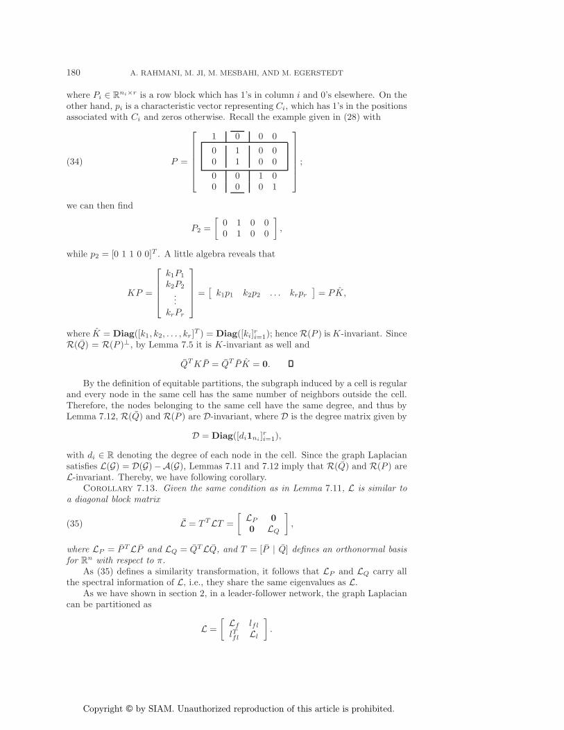
180 A. RAHMANI, M. JI, M. MESBAHI, AND M. EGERSTEDT
where Pi ∈ Rni×r is a row block which has 1’s in column i and 0’s elsewhere. On the
other hand, pi is a characteristic vector representing Ci, which has 1’s in the positionsassociated with Ci and zeros otherwise. Recall the example given in (28) with
(34) P =
⎡⎢⎢⎢⎢⎢⎣
1 0 0 0
0 1 0 00 1 0 0
0 0 1 00 0 0 1
⎤⎥⎥⎥⎥⎥⎦ ;
we can then find
P2 =[
0 1 0 00 1 0 0
],
while p2 = [0 1 1 0 0]T . A little algebra reveals that
KP =
⎡⎢⎢⎢⎣k1P1
k2P2
...krPr
⎤⎥⎥⎥⎦ =
[k1p1 k2p2 . . . krpr
]= PK,
where K = Diag([k1, k2, . . . , kr]T ) = Diag([ki]ri=1); hence R(P ) isK-invariant. SinceR(Q) = R(P )⊥, by Lemma 7.5 it is K-invariant as well and
QTKP = QT P K = 0.
By the definition of equitable partitions, the subgraph induced by a cell is regularand every node in the same cell has the same number of neighbors outside the cell.Therefore, the nodes belonging to the same cell have the same degree, and thus byLemma 7.12, R(Q) and R(P ) are D-invariant, where D is the degree matrix given by
D = Diag([di1ni ]ri=1),
with di ∈ R denoting the degree of each node in the cell. Since the graph Laplaciansatisfies L(G) = D(G)−A(G), Lemmas 7.11 and 7.12 imply that R(Q) and R(P ) areL-invariant. Thereby, we have following corollary.
Corollary 7.13. Given the same condition as in Lemma 7.11, L is similar toa diagonal block matrix
(35) L = T TLT =[ LP 0
0 LQ],
where LP = PTLP and LQ = QTLQ, and T = [P | Q] defines an orthonormal basisfor R
n with respect to π.As (35) defines a similarity transformation, it follows that LP and LQ carry all
the spectral information of L, i.e., they share the same eigenvalues as L.As we have shown in section 2, in a leader-follower network, the graph Laplacian
can be partitioned as
L =[ Lf lfllTfl Ll
].
Copyright © by SIAM. Unauthorized reproduction of this article is prohibited.
CONTROLLABILITY FROM A GRAPH-THEORETIC PERSPECTIVE 181
Transformations similar to (35) can also be found for Lf in the presence of NEPs inthe follower graph Gf .
Corollary 7.14. Let Gf be a follower graph, and let Lf be the diagonal sub-matrix of L related to Gf . If there is an NEP πf in Gf and a π in G such that all thenontrivial cells in πf are also cells in π, then there exists an orthonormal matrix Tfsuch that
(36) Lf = T Tf LfTf =[ LfP 0
0 LfQ].
Proof. Let Pf = Pf (PTf Pf )12 , where Pf is the characteristic matrix for πf .
Moreover, let Qf be defined on an orthonormal basis of R(Pf )⊥. In this way,we obtain an orthonormal basis for R
nf with respect to πf . Moreover, by (9),Lf (G) = Dl
f (G) + L(Gf ), where L(Gf ) denotes the Laplacian matrix of Gf whileDlf is the diagonal follower-leader degree matrix defined in (8). Since all the nontriv-
ial cells in πf are also cells in π, Df satisfies the condition in Lemma 7.12, i.e., nodesfrom an identical cell in πf have the same degree. Hence by Lemma 7.11 and Lemma7.12, R(Pf ) and R(Qf ) are Lf -invariant and consequently,
(37) Lf = T Tf LfTf =[ LfP 0
0 LfQ],
where Tf = [Pf | Qf ], LfP = PTf Lf Pf , and LfQ = QTf Lf Qf .Again, the diagonal blocks of Lf contain the entire spectral information of Lf .
We are now in the position to prove the main result of this section.Theorem 7.15. Given a connected graph G and the induced follower graph Gf ,
the system (7) is not controllable if there exist NEPs on G and Gf , say π and πf ,such that all nontrivial cells of π are contained in πf ; i.e., for all Ci ∈ π\πf , one has|Ci| = 1.
Proof. In Corollaries 7.13 and 7.14, we have shown that L and Lf are similar tosome block diagonal matrices. Here we further expand on the relationship betweensuch matrices.
Assume that π ∩ πf = {C1, C2, . . . , Cr1}. According to the underlying condition,one has |Ci| ≥ 2, i = 1, 2, . . . , r1. Without loss of generality, we can index the nodesin such a way that the nontrivial cells comprise the first n1 nodes, where6
n1 =r1∑i=1
|Ci| ≤ nf < n.
As all the nontrivial cells of π are in πf , their characteristic matrices have similarstructures,
P =[P1 00 In−n1
]n×r
and Pf =[P1 00 Inf−n1
]nf×rf
,
where P1 is an n1 × r1 matrix containing the nontrivial part of the characteristicmatrices. Since P and Pf are the normalizations of P and Pf , respectively, they
6We have introduced n1 for notational convenience. It is easy to verify that n1 − r1 = n − r =nf − rf .
Copyright © by SIAM. Unauthorized reproduction of this article is prohibited.
182 A. RAHMANI, M. JI, M. MESBAHI, AND M. EGERSTEDT
have the same block structures. Consequently Q and Qf , the matrices containing theorthonormal bases of R(P ) and R(Pf ), have the following structures:
Q =[Q1
0
]n×(n1−r1)
and Qf =[Q1
0
]nf×(n1−r1)
,
where Q1 is an n1 × (n1 − r1) matrix that satisfies QT1 P1 = 0. We observe that Qf isdifferent from Q only by n− nf rows of zeros. In other words, the special structuresof Q and Qf lead to the relationship
Qf = RTQ,
where R = [Inf, 0]T . Now, recall the definition of LQ and LQf from (35) and (36),
leading us to
(38) LQ = QTLQ = QTf RTLRQf = QTf Lf Qf = LfQ.
Therefore Lf and L share the same eigenvalues associated with LQ; hence by Lemma7.9, the system is not controllable.
Theorem 7.15 provides a method to identify uncontrollable multi-agent systemsin the presence of multiple leaders. In an uncontrollable multi-agent system, ver-tices in the same cell of an NEP, satisfying the condition in Theorem 7.15, are notdistinguishable from the leaders’ point of view. In other words, agents belonging toa shared cell among π and πf , when identically initialized, remain undistinguishedto the leaders throughout the system evolution. Moreover, the controllable subspacefor this multi-agent system can be obtained by collapsing all the nodes in the samecell into a single “meta-agent.” However, since the NEPs may not be unique, as wehave seen in the case of the Peterson graph, more work is required before a completeunderstanding of the intricate interplay between controllability and NEPs is obtained.
Two immediate ramifications of the above theorem are as follows.Corollary 7.16. Given a connected graph G with the induced follower graph
Gf , a necessary condition for (7) to be controllable is that no NEPs π and πf , on Gand Gf , respectively, share a nontrivial cell.
Corollary 7.17. If G is disconnected, a necessary condition for (7) to be con-trollable is that all of its connected components are controllable.
8. Simulation and discussions. In this section we will explore controllableand uncontrollable leader-follower networks that are amenable to analysis via methodsproposed in this paper.
Example 1 (single leader with symmetric followers). In Figure 6, if we choose node5 as the leader, the symmetric pair (2, 3) in the follower graph renders the networkuncontrollable, as stated in [34]. The dimension of the controllable subspace is three,while there are four nodes in the follower group. This result can also be interpreted viaTheorem 7.15, since the corresponding automorphisms introduce equitable partitions.
Example 2 (single leader with equal distance partitions). We have shown in Fig-ure 5 that the Peterson graph has two NEPs. One is introduced by the automorphismgroup and the other (π2) is introduced by the equal-distance partition. Based on π2,if we choose node 1 as the leader, the leader-follower network ends up with a con-trollable subspace of dimension two. Since there are four orbits in the automorphismgroup,7 this dimension pertains to the two-cell equal-distance partitions.8
7They are {2, 5, 6}, {7, 10}, {8, 9}, and {3, 4}.8They are {2, 5, 6} and {3, 4, 7, 8, 9, 10}.

Copyright © by SIAM. Unauthorized reproduction of this article is prohibited.
CONTROLLABILITY FROM A GRAPH-THEORETIC PERSPECTIVE 183
Fig. 7. A 2-leader network based on the Peterson graph.
Fig. 8. A path-like information exchange network.
Example 3 (multiple leaders). This example is a modified leader graph based onthe Peterson graph. In Figure 7, we add another node (11) connected to {3, 4, 7, 8, 9, 10}as the second leader in addition to node 1. In this network, there is an equal-distancepartition with four cells {1}, {2, 5, 6}, {3, 4, 7, 8, 9, 10}, and {11}. In this case, thedimension of the controllable subspace is still two, which is consistent with the secondexample above.
Example 4 (single-leader controllability). To demonstrate the controllability no-tion for the leader-follower system (7), consider a path-like information network, asshown in Figure 8. In this figure, the last node is chosen as the leader. By Proposition5.17, this system is controllable. The system matrices in (7) assume the form
A =
⎡⎣ −1 1 0
1 −2 10 1 −2
⎤⎦ and B =
⎡⎣ 0
01
⎤⎦ .
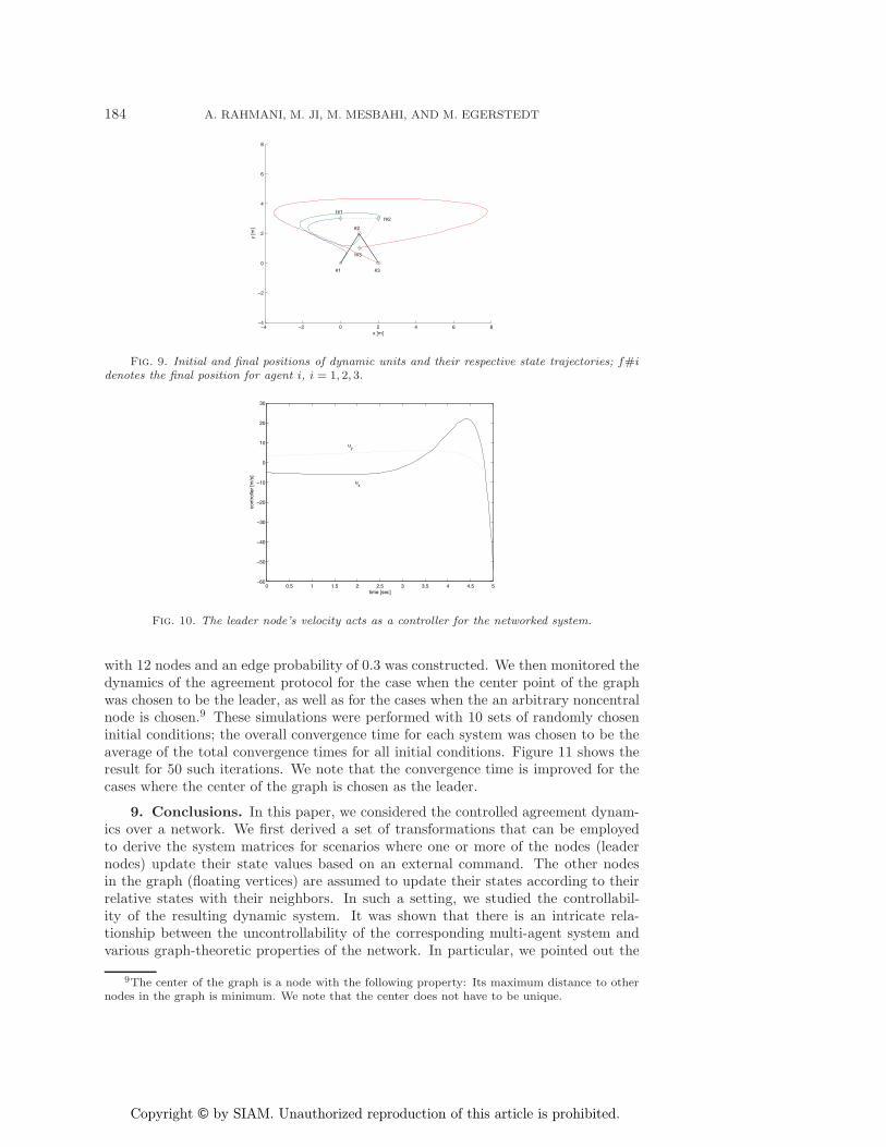
Using (26), one can find the controller that drives the leader-follower system fromany initial state to an arbitrary final state. For this purpose, we chose to re-orientthe planar triangle on the node set {1, 2, 3}. The maneuver time is set to be fiveseconds. Figure 9 shows the initial and the final positions of the nodes along withtheir respective trajectories.
Figure 10, on the other hand, depicts the leader node state trajectory as needed toperform the required maneuver. This trajectory corresponds to the speed of node 4 inthe xy-plane. We note that as there are no restrictions on the leader’s state trajectory,the actual implementation of this control law can become infeasible, especially whenthe maneuver time is arbitrarily short. This observation is apparent in the previousexample, in this scenario, the speed of node 4 changes rather rapidly from 20 [m/s] to−50 [m/s]. To further explore the relationship between the location of the leader nodeand the convergence time to the agreement subspace, an extensive set of simulationswas also carried out. In these simulations, at each step, a random connected graph
Copyright © by SIAM. Unauthorized reproduction of this article is prohibited.
184 A. RAHMANI, M. JI, M. MESBAHI, AND M. EGERSTEDT
Fig. 9. Initial and final positions of dynamic units and their respective state trajectories; f#idenotes the final position for agent i, i = 1, 2, 3.
0 0.5 1 1.5 2 2.5 3 3.5 4 4.5 5−60
−50
−40
−30
−20
−10
0
10
20
30
time [sec]
cont
rolle
r [m
/s]
ux
uy
Fig. 10. The leader node’s velocity acts as a controller for the networked system.
with 12 nodes and an edge probability of 0.3 was constructed. We then monitored thedynamics of the agreement protocol for the case when the center point of the graphwas chosen to be the leader, as well as for the cases when the an arbitrary noncentralnode is chosen.9 These simulations were performed with 10 sets of randomly choseninitial conditions; the overall convergence time for each system was chosen to be theaverage of the total convergence times for all initial conditions. Figure 11 shows theresult for 50 such iterations. We note that the convergence time is improved for thecases where the center of the graph is chosen as the leader.
9. Conclusions. In this paper, we considered the controlled agreement dynam-ics over a network. We first derived a set of transformations that can be employedto derive the system matrices for scenarios where one or more of the nodes (leadernodes) update their state values based on an external command. The other nodesin the graph (floating vertices) are assumed to update their states according to theirrelative states with their neighbors. In such a setting, we studied the controllabil-ity of the resulting dynamic system. It was shown that there is an intricate rela-tionship between the uncontrollability of the corresponding multi-agent system andvarious graph-theoretic properties of the network. In particular, we pointed out the
9The center of the graph is a node with the following property: Its maximum distance to othernodes in the graph is minimum. We note that the center does not have to be unique.

Copyright © by SIAM. Unauthorized reproduction of this article is prohibited.
CONTROLLABILITY FROM A GRAPH-THEORETIC PERSPECTIVE 185
0 10 20 30 40 500
20
40
60
80
100
120
iteration #
conv
erge
nce
time
[sec
]
Fig. 11. Convergence time comparison (x: center node is the leader. o: an arbitrary noncentralpoint is the leader).
importance of the network automorphism group and its nontrivial equitable partitionsin the controllability properties of the interconnected system. Some of the ramifica-tions of this correspondence were then explored. The results of the present workpoint to a promising research direction at the intersection of graph theory and controltheory that aims to study system-theoretic attributes from a purely graph-theoreticoutlook.
Acknowledgments. The authors would like to thank the referees for their help-ful comments and suggestions.
REFERENCES
[1] T. Balch and R. C. Arkin, Behavior-based formation control for multi-robot teams, IEEETrans. Robotics Automat., 14 (1998), pp. 926–939.
[2] B. Bamieh, F. Paganini, and M. Dahleh, Distributed control of spatially-invariant systems,IEEE Trans. Automat. Control, 47 (2002), pp. 1091–1107.
[3] R. W. Beard, J. R. Lawton, and F. Y. Hadaegh, A coordination architecture for spacecraftformation control, IEEE Trans. Control Systems Technology, 9 (2001), pp. 777–790.
[4] D. P. Bertsekas and J. N. Tsitsiklis, Parallel and Distributed Computation, Prentice–Hall,Englewood Cliffs, NJ, 1989.
[5] N. Biggs, Algebraic Graph Theory, Cambridge University Press, Cambridge, UK, 1993.[6] B.-D. Chen and S. Lall, Dissipation inequalities for distributed systems on graphs, in Pro-
ceedings of the 42nd IEEE Conference on Decision and Control, IEEE Press, Piscataway,NJ, 2003 pp. 3084–3090.
[7] J. Cortes and F. Bullo, Coordination and geometric optimization via distributed dynamicalsystems, SIAM J. Control Optim., 44 (2005), pp. 1543–1574.
[8] J. Cortes, S. Martınez, and F. Bullo, Robust rendezvous for mobile autonomous agentsvia proximity graphs in arbitrary dimensions, IEEE Trans. Automat. Control, 8 (2006),pp. 1289–1298.
[9] R. D’Andrea and G. E. Dullerud, Distributed control design for spatially interconnectedsystems, IEEE Trans. Automat. Control, 9 (2003), pp. 1478–1495.
[10] J. Desai, J. Ostrowski, and V. Kumar, Controlling formations of multiple mobile robots,in Proceedings of the IEEE International Conference on Robotics and Automation, IEEEPress, Piscataway, NJ, 1998, pp. 2864–2869.
[11] R. Diestel, Graph Theory, Springer, New York, 2000.[12] C. Fall, E. Marland, J. Wagner, and J. Tyson, eds., Computational Cell Biology, Springer,
New York, 2005.

Copyright © by SIAM. Unauthorized reproduction of this article is prohibited.
186 A. RAHMANI, M. JI, M. MESBAHI, AND M. EGERSTEDT
[13] J. Fax and R. Murray, Information flow and cooperative control of vehicle formations, IEEETrans. Automat. Control, 49 (2004), pp. 1465–1476.
[14] C. Godsil and G. Royle, Algebraic Graph Theory, Springer, New York, 2001.[15] Y. Hatano and M. Mesbahi, Agreement over random networks, IEEE Trans. Automat. Con-
trol, 50 (2005), pp. 1867–1872.[16] R. A. Horn and C. Johnson, Matrix Analysis, Cambridge University Press, Cambridge, UK,
1985.[17] A. Jadbabaie, J. Lin, and A. S. Morse, Coordination of groups of mobile autonomous agents
using nearest neighbor rules, IEEE Trans. Automat. Control, 6 (2003), pp. 988–1001.[18] M. Ji, A. Muhammad, and M. Egerstedt, Leader-based multi-agent coordination: Controlla-
bility and optimal control, in Proceedings of the IEEE American Control Conference, IEEEPress, Piscataway, NJ, 2006, article 1656406.
[19] T. Kailath, Linear Systems, Prentice–Hall, Englewood Cliffs, NJ, 1980.[20] Y. Kim, M. Mesbahi, and F. Y. Hadaegh, Multiple-spacecraft reconfigurations through colli-
sion avoidance, bouncing, and stalemates, J. Optim. Theory Appl., 2 (2004), pp. 323–343.[21] J. Lauri and R. Scapellato, Topics in Graph Automorphisms and Reconstruction, Cam-
bridge University Press, Cambridge, UK, 2003.[22] Z. Lin, M. Broucke, and B. Francis, Local control strategies for groups of mobile autonomous
agents, IEEE Trans. Automat. Control, 4 (2004), pp. 622–629.[23] D. Luenberger, Optimization by Vector Space Methods, Wiley, New York, 1969.[24] R. Merris, Laplacian matrices of graphs: A survey, Linear Algebra Appl., 197 (1994), pp. 143–
176.[25] M. Mesbahi, State-dependent graphs, in Proceedings of the 42nd IEEE Conference on Decision
and Control, IEEE Press, Piscataway, NJ, 2003, pp. 3058–3063.[26] M. Mesbahi, State-dependent graphs and their controllability properties, IEEE Trans. Automat.
Control, 3 (2005), pp. 387–392.[27] M. Mesbahi and F. Y. Hadaegh, Formation flying control of multiple spacecraft via graphs,
matrix inequalities, and switching, J. Guidance Control Dynam., 2 (2001), pp. 369–377.[28] L. Moreau, Stability of multiagent systems with time-dependent communication links, IEEE
Trans. Automat. Control, 2 (2005), pp. 169–182.[29] R. Olfati-Saber and R. M. Murray, Agreement problems in networks with directed graphs
and switching topology, in Proceedings of the 42nd IEEE Conference on Decision andControl, IEEE Press, Piscataway, NJ, 2003, pp. 4126–4132.
[30] R. Olfati-Saber and R. M. Murray, Consensus problems in networks of agents with switch-ing topology and time-delays, IEEE Trans. Automat. Control, 9 (2004), pp. 1520–1533.
[31] R. Olfati-Saber and J. S. Shamma, Consensus filters for sensor networks and distributedsensor fusion, in Proceedings of the 44th IEEE Conference on Decision and Control, IEEEPress, Piscataway, NJ, 2005, pp. 6698–6703.
[32] R. Olfati-Saber, Flocking for multi-agent dynamic systems: Algorithms and theory, IEEETrans. Automat. Control, 3 (2006), pp. 401–420.
[33] K. Ogata, Modern Control Engineering, Prentice–Hall, Upper Saddle River, NJ, 2002.[34] A. Rahmani and M. Mesbahi, On the controlled agreement problem, in Proceedings of the
IEEE American Control Conference, IEEE Press, Piscataway, NJ, 2006, article 1656409.[35] H. Tanner, A. Jadbabaie, and G. Pappas, Stable flocking of mobile agents, part II: Dynamic
topology, in Proceedings of the 42nd IEEE Conference on Decision and Control, IEEEPress, Piscataway, NJ, 2003, pp. 2016–2021.
[36] H. G. Tanner, On the controllability of nearest neighbor interconnections, in Proceedings ofthe 43rd IEEE Conference on Decision and Control, IEEE Press, Piscataway, NJ, 2004,pp. 2467–2472.
[37] G. Walsh, H. Ye, and L. Bushnell, Stability analysis of networked control systems, in Pro-ceedings of the American Control Conference, IEEE Press, Piscataway, NJ, 1999, pp. 2876–2880.
[38] P. K. C. Wang and F. Y. Hadaegh, Coordination and control of multiple microspacecraftmoving in formation, J. Astronautical Sci., 44 (1996), pp. 315–355.
[39] L. Xiao and S. Boyd, Fast linear iterations for distributed averaging, Systems Control Lett.,53 (2004), pp. 65–78.