Controllability of Fokker-Planck equations and the ...porretta/MCT-Trieste.pdf · Controllability of Fokker-Planck equations and the ... A similar paradygm independently developed

Controllability of Fokker-Planck equations and theplanning problem for mean field games

Alessio PorrettaUniversita’ di Roma Tor Vergata

Mathematical Control in Trieste, 3/12/2013

A. Porretta The planning problem for mean field games

Outlines of the talk

Brief description of the Mean Field Games model.Coupling viscous Hamilton-Jacobi & Fokker-Planck equations.

The planning problem: a question of optimal transport & optimalcontrol.

Construction of the solution as limit of standard mean field gamesproblems (from optimal control to exact controllability).

Uniqueness of weak solutions

Comments, work in progress and perspectives.


Mean Field Games

The Mean Field Games model was introduced by Lasry-Lions since 2006.A similar paradygm independently developed by Huang-Caines-Malhamein terms of stochastic dynamics.

Main goal: describe games with large numbers (a continuum) of agentswhose strategies depend on the distribution of the other agents.

Typical features of the model:

- players act according to the same principles (they are indistinguishableand have the same optimization criteria).

- players have individually a minor (infinitesimal) influence, but theirstrategy takes into account the mass of co-players.

Roughly: players are particles but have strategies (more sophisticatedthan particle physics or similar economics models); however, they onlyconsider the statistical state of the mass of co-players (less sophisticatedthan agents of N-players games)

Goal: introduce a macroscopic description through a mean field approachas the number of players N →∞.


The simplest form of the continuum limit is a coupled system of PDEs(1) −ut −∆u + H(x ,Du) = F (x ,m) in (0,T )× Ω

(2) mt −∆m − div(mHp(x ,Du)) = 0 in (0,T )× Ω ,

where Hp stands for ∂H(x,p)∂p .

(1) is the Bellman equation for the agents’ value function u.

(2) is the Kolmogorov-Fokker-Planck equation for the state of theagents. m(t) is the probability density of the state of players attime t.


Roughly, each agent controls the dynamics of a N-d Brownian motion

dXt = βtdt +√

2dBt ,

in order to minimize, among controls βt , some cost:

inf J(β) := E

∫ T

0

[L(Xs , βs) + F (Xs ,m(s))]ds + G (XT ,m(T ))

where m(t) is the probability measure in RN induced by the law of theprocess Xt .

The associated Hamilton-Jacobi-Bellman equation is

−ut −∆u + H(x ,Du) = F (x ,m(t))

where H = supβ[−β · p − L(x , β)].

If u solves the Bellman equation it gives

• the best value infβ J(β) =∫u(x , 0)dm0(x),

where m0 is the probability distribution of X0.

• the optimal feedback β∗t =b(t,Xt), where b(t, x) = −Hp(x ,Du(t, x))A. Porretta The planning problem for mean field games

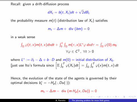
Recall: given a drift-diffusion process

dXt = b(t,Xt)dt +√

2dBt

the probability measure m(t) (distribution law of Xt) satisfies

mt −∆m + div (bm) = 0

in a weak sense∫Ωϕ(t, x)m(t, x)dxdt +

∫ t

0

∫Ωm(τ, x)L∗ϕ dxdτ =

∫Ωϕ(0)m0

∀ϕ ∈ C 2 , ∀t > 0

where L∗ := ∂t −∆ + b · D and m(0) = initial distribution of X0.

[just use Ito’s formula since[E∫ T

0ϕ(Xt)dt

]=∫

Ω

∫ T

0ϕ(x)m(t, x) dt

Hence, the evolution of the state of the agents is governed by theiroptimal decisions b∗t = −Hp(·,Du(·)):

mt −∆m − div (mHp(x ,Du)) = 0


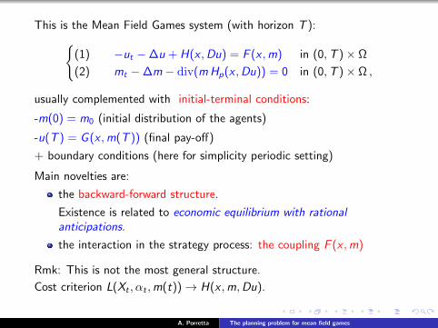
This is the Mean Field Games system (with horizon T ):(1) −ut −∆u + H(x ,Du) = F (x ,m) in (0,T )× Ω

(2) mt −∆m − div(mHp(x ,Du)) = 0 in (0,T )× Ω ,

usually complemented with initial-terminal conditions:

-m(0) = m0 (initial distribution of the agents)

-u(T ) = G (x ,m(T )) (final pay-off)

+ boundary conditions (here for simplicity periodic setting)

Main novelties are:

the backward-forward structure.

Existence is related to economic equilibrium with rationalanticipations.

the interaction in the strategy process: the coupling F (x ,m)

Rmk: This is not the most general structure.

Cost criterion L(Xt , αt ,m(t))→ H(x ,m,Du).


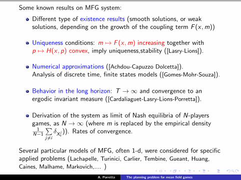
Some known results on MFG system:

Different type of existence results (smooth solutions, or weaksolutions, depending on the growth of the coupling term F (x ,m))

Uniqueness conditions: m 7→ F (x ,m) increasing together withp 7→ H(x , p) convex, imply uniqueness,stability ([Lasry-Lions]).

Numerical approximations ([Achdou-Capuzzo Dolcetta]).Analysis of discrete time, finite states models ([Gomes-Mohr-Souza]).

Behavior in the long horizon: T →∞ and convergence to anergodic invariant measure ([Cardaliaguet-Lasry-Lions-Porretta]).

Derivation of the system as limit of Nash equilibria of N-playersgames, as N →∞ (where m is replaced by the empirical density

1N−1

∑j 6=i

δX js)). Rates of convergence.

Several particular models of MFG, often 1-d, were considered for specificapplied problems (Lachapelle, Turinici, Carlier, Tembine, Gueant, Huang,

Caines, Malhame, Markovich,.... )


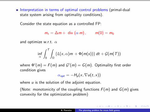
Interpretation in terms of optimal control problems (primal-dualstate system arising from optimality conditions).

Consider the state equation as a controlled FP:

mt = ∆m + div (αm) , m(0) = m0

and optimize w.r.t. α

infα

∫ T

0

∫Ω

L(x , α)m + Φ(m(s)) dt + G(m(T ))

where Φ′(m) = F (m) and G′(m) = G (m). Optimality first ordercondition gives

αopt = −Hp(x ,∇u(t, x))

where u is the solution of the adjoint equation.

(Note: monotonicity of the coupling functions F (m) and G (m) givesconvexity for the optimization problem)


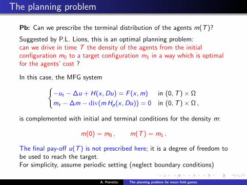
The planning problem

Pb: Can we prescribe the terminal distribution of the agents m(T )?

Suggested by P.L. Lions, this is an optimal planning problem:can we drive in time T the density of the agents from the initialconfiguration m0 to a target configuration m1 in a way which is optimalfor the agents’ cost ?

In this case, the MFG system−ut −∆u + H(x ,Du) = F (x ,m) in (0,T )× Ω

mt −∆m − div(mHp(x ,Du)) = 0 in (0,T )× Ω ,

is complemented with initial and terminal conditions for the density m:

m(0) = m0 , m(T ) = m1 .

The final pay-off u(T ) is not prescribed here; it is a degree of freedom tobe used to reach the target.For simplicity, assume periodic setting (neglect boundary conditions)


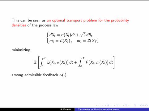
This can be seen as an optimal transport problem for the probabilitydensities of the process law

dXt = α(Xt)dt +√

2 dBt

m0 = L(X0) , m1 = L(XT )

minimizing

E

[∫ T

0

L(Xt , α(Xt)) dt +

∫ T

0

F (Xt ,m(Xt)) dt

]

among admissible feedback α(·).


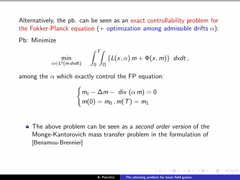
Alternatively, the pb. can be seen as an exact controllability problem forthe Fokker-Planck equation (+ optimization among admissible drifts α):

Pb: Minimize

minα∈L2(m dxdt)

∫ T

0

∫Ω

L(x , α)m + Φ(x ,m) dxdt ,

among the α which exactly control the FP equation:mt −∆m − div (αm) = 0

m(0) = m0 ,m(T ) = m1

The above problem can be seen as a second order version of theMonge-Kantorovich mass transfer problem in the formulation of[Benamou-Brennier]


The model case H(x ,Du) = 12 |Du|

2 was solved by P.L. Lions:

-F (m) nondecreasing and bounded, m0, m1 smooth and positive:

m0,m1 ∈ C 1(Ω) , m0,m1 > 0,

∫Ω

m0 dx =

∫Ω

m1 dx = 1

Then, there exists a smooth solution (u,m) to−ut −∆u + 1

2 |Du|2 = F (m) in (0,T )× Ω

mt −∆m − div(mDu) = 0 in (0,T )× Ω ,

m(0) = m0 , m(T ) = m1 ,

+periodic b.c.

Moreover, the smooth solution is unique (up to adding a constant to u).

Lions’ proof relies on a change of unknown, including the Hopf-Coletransform, which reduces the pb. to a semilinear system:

ϕ := e−12 u ; ψ := me

12 u

⇒

−ϕt −∆ϕ+ 1

2F (x , ϕψ)ϕ = 0

ψt −∆ψ + 12F (x , ϕψ)ψ = 0


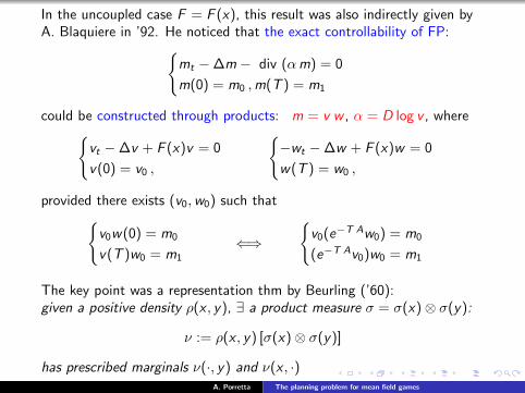
In the uncoupled case F = F (x), this result was also indirectly given byA. Blaquiere in ’92. He noticed that the exact controllability of FP:

mt −∆m − div (αm) = 0

m(0) = m0 ,m(T ) = m1

could be constructed through products: m = v w , α = D log v , wherevt −∆v + F (x)v = 0

v(0) = v0 ,

−wt −∆w + F (x)w = 0

w(T ) = w0 ,

provided there exists (v0,w0) such thatv0w(0) = m0

v(T )w0 = m1

⇐⇒

v0(e−T Aw0) = m0

(e−T Av0)w0 = m1

The key point was a representation thm by Beurling (’60):given a positive density ρ(x , y), ∃ a product measure σ = σ(x)⊗ σ(y):

ν := ρ(x , y) [σ(x)⊗ σ(y)]

has prescribed marginals ν(·, y) and ν(x , ·)A. Porretta The planning problem for mean field games

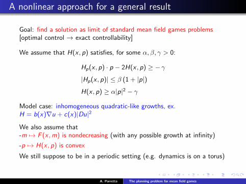
A nonlinear approach for a general result

Goal: find a solution as limit of standard mean field games problems[optimal control → exact controllability]

We assume that H(x , p) satisfies, for some α, β, γ > 0:

Hp(x , p) · p − 2H(x , p) ≥ − γ

|Hp(x , p)| ≤ β (1 + |p|)

H(x , p) ≥ α|p|2 − γ

Model case: inhomogeneous quadratic-like growths, ex.H = b(x)∇u + c(x)|Du|2

We also assume that-m 7→ F (x ,m) is nondecreasing (with any possible growth at infinity)

-p 7→ H(x , p) is convex

We still suppose to be in a periodic setting (e.g. dynamics is on a torus)


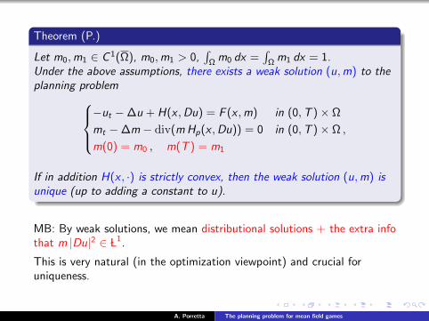
Theorem (P.)

Let m0,m1 ∈ C 1(Ω), m0,m1 > 0,∫

Ωm0 dx =

∫Ωm1 dx = 1.

Under the above assumptions, there exists a weak solution (u,m) to theplanning problem

−ut −∆u + H(x ,Du) = F (x ,m) in (0,T )× Ω

mt −∆m − div(mHp(x ,Du)) = 0 in (0,T )× Ω ,

m(0) = m0 , m(T ) = m1

If in addition H(x , ·) is strictly convex, then the weak solution (u,m) isunique (up to adding a constant to u).

MB: By weak solutions, we mean distributional solutions + the extra infothat m |Du|2 ∈ L1.

This is very natural (in the optimization viewpoint) and crucial foruniqueness.


Comments & remarks:

Compared with P.-L. Lions’ result, we obtain only weak solutions(smoothness ? open problem). Nevertheless, weak solutions areunique!

Our approach only relies on energy methods (estimates,compactness); we construct the solution from penalized optimalcontrol problems, as it is customary for exact controllability.

Numerical schemes were studied in [Achdou-Camilli-Capuzzo Dolcetta

’12] (consistency, existence for the discretized problem).

This was our starting motivation: find the arguments (at thecontinuous level) which may be used for the convergence ofnumerical approximations.


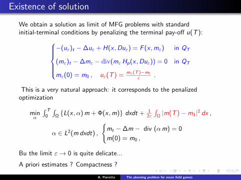
Existence of solution

We obtain a solution as limit of MFG problems with standardinitial-terminal conditions by penalizing the terminal pay-off u(T ):

−(uε)t −∆uε + H(x ,Duε) = F (x ,mε) in QT

(mε)t −∆mε − div(mε Hp(x ,Duε)) = 0 in QT

mε(0) = m0 , uε(T ) = mε(T )−m1

ε .

This is a very natural approach: it corresponds to the penalizedoptimization

minα

∫ T

0

∫ΩL(x , α)m + Φ(x ,m) dxdt + 1

2ε

∫Ω|m(T )−m1|2 dx ,

α ∈ L2(mdxdt) ,

mt −∆m − div (αm) = 0

m(0) = m0 ,

Bu the limit ε→ 0 is quite delicate...

A priori estimates ? Compactness ?


Part I. Estimates.

We use several tools among which some structural points of MFG system:

1. The structure of Hamiltonian system:

−ut −∆u + H(x ,Du) = F (x ,m)

mt −∆m − div(mHp(x ,Du)) = 0⇐⇒

∂u

∂t=∂E∂m

∂m

∂t= −∂E

∂u

where

E(u,m) =

∫Ω

[1

2m|∇u|2 +∇u · ∇m − Φ(x ,m)]dx

In particular, the quantity E(u(t),m(t)) is constant along the flow.

2. This gives a kind of observability inequality: any solution satisfies∫Ω

|Du(0)|2 dx ≤ C

∫ T

0

∫Ω

m |Du|2 dxdt + 1

(1)

where C = C (T ,H,m0).


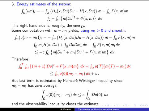
3. Energy estimates of the system:∫Ω

(um)t = −∫

ΩHp(x ,Du)Du − H(x ,Du)m −

∫ΩF (x ,m)m

. −∫

Ω

m|Du|2 + Φ(x ,m)

dx

The right hand side is, roughly, the energy.Same computation with m −m1 yields, using m1 > 0 and smooth:∫

Ω(u(m −m1))t = −

∫ΩHp(x ,Du)Du − H(x ,Du)m −

∫ΩF (x ,m)m

−∫

Ωm1H(x ,Du) +

∫ΩDuDm1 dx −

∫ΩF (x ,m)m1dx

. −c∫

Ω

m|Du|2 + m1|Du|2 + F (x ,m)m

dx

Therefore∫ T

0

∫Ω

(m + 1)|Du|2 + F (x ,m)m

dx +

∫Ωu(T )(m(T )−m1)dx

≤∫

Ωu(0)(m0 −m1) dx + c .

But last term is estimated by Poincare-Wirtinger inequality sincem0 −m1 has zero average:∫

Ω

u(0)(m0 −m1) dx ≤ c

∫Ω

|Du(0)| dx

and the observability inequality closes the estimateA. Porretta The planning problem for mean field games

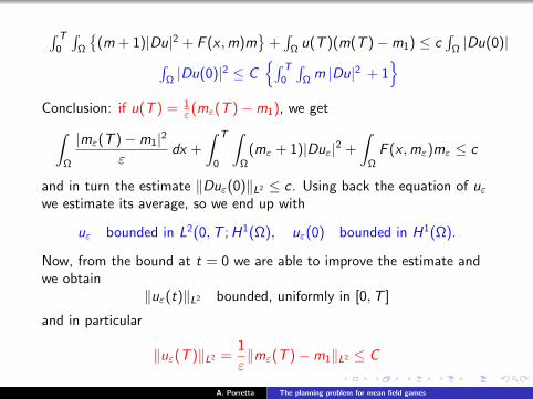
∫ T

0

∫Ω

(m + 1)|Du|2 + F (x ,m)m

+∫

Ωu(T )(m(T )−m1) ≤ c

∫Ω|Du(0)|∫

Ω|Du(0)|2 ≤ C

∫ T

0

∫Ωm |Du|2 + 1

Conclusion: if u(T ) = 1

ε (mε(T )−m1), we get∫Ω

|mε(T )−m1|2

εdx +

∫ T

0

∫Ω

(mε + 1)|Duε|2 +

∫Ω

F (x ,mε)mε ≤ c

and in turn the estimate ‖Duε(0)‖L2 ≤ c . Using back the equation of uεwe estimate its average, so we end up with

uε bounded in L2(0,T ;H1(Ω), uε(0) bounded in H1(Ω).

Now, from the bound at t = 0 we are able to improve the estimate andwe obtain

‖uε(t)‖L2 bounded, uniformly in [0,T ]

and in particular

‖uε(T )‖L2 =1

ε‖mε(T )−m1‖L2 ≤ C


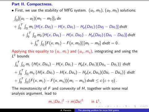
Part II. Compactness.

• First, we use the stability of MFG system. (u1,m1), (u2,m2) solutions:∫Ω

[(u1 − u2)(m1 −m2)]t dx

+∫ T

0

∫Ωm1 [H(x ,Du2)− H(x ,Du1)− Hp(Du1) (Du2 − Du1)] dxdt

+∫ T

0

∫Ωm2 [H(x ,Du1)− H(x ,Du2)− Hp(Du2) (Du1 − Du2)] dxdt

+∫ T

0

∫Ω

[F (x ,m1)− F (x ,m2)] [m1 −m2] dxdt = 0 .

Applying this equality to (uε,mε) and (uη,mη), integrating and using theL2 bounds∫ T

0

∫Ωmε H(x ,Duη)− H(x ,Duε)− Hp(x ,Duε)(Duη − Duε) dxdt

+∫ T

0

∫Ωmη H(x ,Duε)− H(x ,Duη)− Hp(x ,Duη)(Duε − Duη) dxdt

+∫ T

0

∫Ω

(F (x ,mε)− F (x ,mη))(mε −mη) dxdt ≤ c (ε+ η) .

The monotonicity of F and convexity of H, together with some realanalysis argument, lead to

mε|Duε|2 → m|Du|2 in L1.


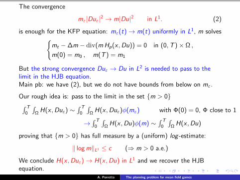
The convergence

mε|Duε|2 → m|Du|2 in L1. (2)

is enough for the KFP equation: mε(t)→ m(t) uniformly in L1, m solvesmt −∆m − div(mHp(x ,Du)) = 0 in (0,T )× Ω ,

m(0) = m0 , m(T ) = m1

But the strong convergence Duε → Du in L2 is needed to pass to thelimit in the HJB equation.Main pb: we have (2), but we do not have bounds from below on mε.

Our rough idea is: pass to the limit in the set m > 0∫ T

0

∫ΩH(x ,Duε) ∼

∫ T

0

∫ΩH(x ,Duε)φ(mε) with Φ(0) = 0, Φ close to 1

→∫ T

0

∫ΩH(x ,Du)φ(m) ∼

∫ T

0

∫ΩH(x ,Du)

proving that m > 0 has full measure by a (uniform) log -estimate:

‖ logm‖L1 ≤ c (⇒ m > 0 a.e.)

We conclude H(x ,Duε)→ H(x ,Du) in L1 and we recover the HJBequation.


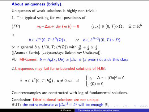
About uniqueness (briefly).

Uniqueness of weak solutions is highly non trivial:

1. The typical setting for well-posedness of

(FP) mt−∆m+ div (mb) = 0 (t, x) ∈ (0,T )×Ω , Ω ⊂ RN

isb ∈ L∞(0,T ; LN(Ω)) , or b ∈ LN+2((0,T )× Ω)

or in general b ∈ Lr (0,T ; Lq(Ω)) with N2r + 1

q ≤12

([Aronson-Serrin], [Ladysenskaya-Solonnikov-Uraltseva]).

Pb. MFGames: b = Hp(x ,Du) ' |Du| is (a priori) outside this class

2.Uniqueness may fail for unbounded solutions of HJB:

∃ u ∈ L2(0,T ;H10 ) , u 6= 0 sol. of

ut −∆u + |Du|2 = 0

u(0) = 0

Counterexamples are constructed with log of fundamental solutions.

Conclusion: Distributional solutions are not unique.BUT: the extra estimate m |Du|2 ∈ L1 will be enough !!!


Uniqueness stands on the following two main steps:

1. New results on weak solutions of Fokker-Planck equations.

Key-point: we can consider solutions of Fokker-Planck

mt −∆m − div (bm) = 0

such that m ≥ 0, m|b|2 ∈ L1

In this framework, we can prove:

1 Weak (=distributional) solutions of (FP) are unique in this class(see also [Bogachev-Da Prato-Rockner ’11])

2 Weak solutions are renormalized solutions;

(in the sense of [Di Perna-Lions], [Lions-Murat])

Moreover, we show that solutions can be regularized and obtained aslimit of smooth solutions.


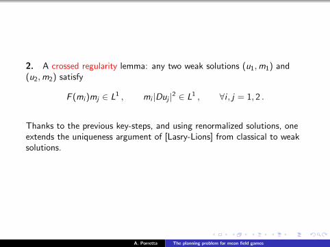
2. A crossed regularity lemma: any two weak solutions (u1,m1) and(u2,m2) satisfy

F (mi )mj ∈ L1 , mi |Duj |2 ∈ L1 , ∀i , j = 1, 2 .

Thanks to the previous key-steps, and using renormalized solutions, oneextends the uniqueness argument of [Lasry-Lions] from classical to weaksolutions.


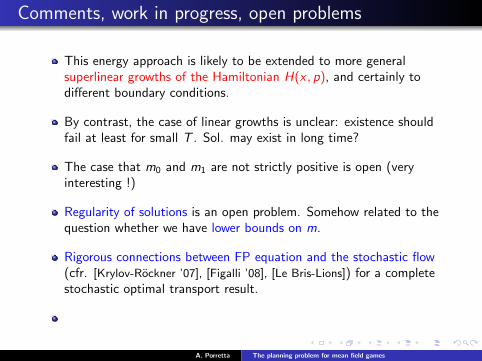
Comments, work in progress, open problems

This energy approach is likely to be extended to more generalsuperlinear growths of the Hamiltonian H(x , p), and certainly todifferent boundary conditions.

By contrast, the case of linear growths is unclear: existence shouldfail at least for small T . Sol. may exist in long time?

The case that m0 and m1 are not strictly positive is open (veryinteresting !)

Regularity of solutions is an open problem. Somehow related to thequestion whether we have lower bounds on m.

Rigorous connections between FP equation and the stochastic flow(cfr. [Krylov-Rockner ’07], [Figalli ’08], [Le Bris-Lions]) for a completestochastic optimal transport result.


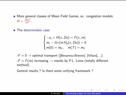
More general classes of Mean Field Games, ex. congestion models:

H = |Du|2mγ .

The deterministic case:−ut + H(x ,Du) = F (x ,m)

mt − div(mHp(x ,Du)) = 0

m(0) = m0 , m(T ) = m1

-F = 0→ optimal transport ([Benamou-Brenier], [Villani],...).

-F = F (m) increasing → results by P.L. Lions (totally differentmethod).

General results ? Is there some unifying framework ?


Thanks for the attention !


Documents

Controllability of Fokker-Planck equations and the ...porretta/MCT-Trieste.pdf · Controllability of Fokker-Planck equations and the ... A similar paradygm independently developed