Embed Size (px)
Citation preview

Controllability of Complex Networks
Yang-Yu Liu
Center of Complex Network ResearchNortheastern University
May 2011
Tuesday, May 3, 2011

Collaborators
Jean-Jacques SlotineMIT
Albert-László BarabásiNEU/HMS
Tuesday, May 3, 2011

NATURE.COM/NATURE12 May 2011 £10
Vol. 473, No. 7346
POLICY
WHO NEEDS CHANGE
A World Health Organization for today’s world
PAGE !43
MICROBIOLOGY
A BOOST FOR ANTIBIOTICS
How metabolic ‘helpers’ kill persistent pathogens
PAGE XXX
GEOLOGY
WAITING FOR THE INEVITABLEVesuvius will erupt again —
but when?PAGE !40
TAMING COMPLEXITYThe mathematics of network control — from
cell biology to cellphones PAGES XXX & XXX
T H E I N T E R N AT I O N A L W E E K LY J O U R N A L O F S C I E N C E
ARTICLEdoi:10.1038/nature10011
Controllability of complex networksYang-Yu Liu1,2, Jean-Jacques Slotine3,4 & Albert-Laszlo Barabasi1,2,5
The ultimate proof of our understanding of natural or technological systems is reflected in our ability to control them.Although control theory offersmathematical tools for steering engineered and natural systems towards a desired state, aframework to control complex self-organized systems is lacking. Here we develop analytical tools to study thecontrollability of an arbitrary complex directed network, identifying the set of driver nodes with time-dependentcontrol that can guide the system’s entire dynamics. We apply these tools to several real networks, finding that thenumber of driver nodes is determined mainly by the network’s degree distribution. We show that sparseinhomogeneous networks, which emerge in many real complex systems, are the most difficult to control, but thatdense and homogeneous networks can be controlled using a few driver nodes. Counterintuitively, we find that inboth model and real systems the driver nodes tend to avoid the high-degree nodes.
According to control theory, a dynamical system is controllable if, with asuitable choice of inputs, it can be driven from any initial state to anydesired final state within finite time1–3. This definition agrees with ourintuitive notion of control, capturing an ability to guide a system’sbehaviour towards adesired state through the appropriatemanipulationof a few input variables, like a driver prompting a car to move with thedesired speed and in the desired direction by manipulating the pedalsand the steering wheel. Although control theory is a mathematicallyhighly developed branch of engineering with applications to electriccircuits, manufacturing processes, communication systems4–6, aircraft,spacecraft and robots2,3, fundamental questions pertaining to the con-trollability of complex systems emerging in nature and engineering haveresisted advances. The difficulty is rooted in the fact that two independ-ent factors contribute to controllability, each with its own layer ofunknown: (1) the system’s architecture, represented by the networkencapsulating which components interact with each other; and (2) thedynamical rules that capture the time-dependent interactions betweenthe components. Thus, progress has beenpossible only in systemswhereboth layers are well mapped, such as the control of synchronized net-works7–10, small biological circuits11 and rate control for communica-tion networks4–6. Recent advances towards quantifying the topologicalcharacteristics of complex networks12–16 have shed light on factor (1),prompting us to wonder whether some networks are easier to controlthan others and how network topology affects a system’s controllability.Despite some pioneering conceptual work17–23 (SupplementaryInformation, section II), we continue to lack general answers to thesequestions for large weighted and directed networks, which most com-monly emerge in complex systems.
Network controllabilityMost real systems are driven by nonlinear processes, but the controll-ability of nonlinear systems is in many aspects structurally similar tothat of linear systems3, prompting us to start our study using thecanonical linear, time-invariant dynamics
dx(t)dt
~Ax(t)zBu(t) !1"
where the vector x(t)5 (x1(t), …, xN(t))T captures the state of a
system ofN nodes at time t. For example, xi(t) can denote the amount
of traffic that passes through a node i in a communication network24
or transcription factor concentration in a gene regulatory network25.The N3N matrix A describes the system’s wiring diagram and theinteraction strength between the components, for example the trafficon individual communication links or the strength of a regulatoryinteraction. Finally, B is the N3M input matrix (M#N) that iden-tifies the nodes controlled by an outside controller. The system iscontrolled using the time-dependent input vector u(t)5 (u1(t), …,uM(t))
T imposed by the controller (Fig. 1a), where in general the samesignal ui(t) can drivemultiple nodes. If wewish to control a system, wefirst need to identify the set of nodes that, if driven by different signals,can offer full control over the network. We will call these ‘drivernodes’. We are particularly interested in identifying the minimumnumber of driver nodes, denoted by ND, whose control is sufficientto fully control the system’s dynamics.The system described by equation (1) is said to be controllable if it
can be driven from any initial state to any desired final state in finitetime, which is possible if and only if theN3NM controllability matrix
C~(B,AB,A2B, . . . ,AN{1B) !2"
has full rank, that is
rank(C)~N !3"
This represents the mathematical condition for controllability, and iscalled Kalman’s controllability rank condition1,2 (Fig. 1a). In practicalterms, controllability canbe alsoposed as follows. Identify theminimumnumber of driver nodes such that equation (3) is satisfied. For example,equation (3) predicts that controlling node x1 in Fig. 1b with the inputsignalu1 offers full controlover the system, as the states of nodesx1,x2,x3and x4 are uniquely determined by the signal u1(t) (Fig. 1c). In contrast,controlling the top node in Fig. 1e is not sufficient for full control, as thedifference a31x2(t)2 a21x3(t) (where aij are the elements of A) is notuniquely determined by u1(t) (see Fig. 1f and SupplementaryInformation section III.A). To gain full control, wemust simultaneouslycontrol node x1 and any two nodes among {x2, x3, x4} (see Fig. 1h, i for amore complex example).To apply equations (2) and (3) to an arbitrary network, we need to
know the weight of each link (that is, the aij), which for most real
1Center for Complex Network Research and Departments of Physics, Computer Science and Biology, Northeastern University, Boston, Massachusetts 02115, USA. 2Center for Cancer Systems Biology,Dana-Farber Cancer Institute, Boston, Massachusetts 02115, USA. 3Nonlinear Systems Laboratory, Massachusetts Institute of Technology, Cambridge, Massachusetts 02139, USA. 4Department ofMechanical EngineeringandDepartmentofBrain andCognitiveSciences,Massachusetts Institute of Technology, Cambridge,Massachusetts02139,USA. 5DepartmentofMedicine,BrighamandWomen’sHospital, Harvard Medical School, Boston, Massachusetts 02115, USA.
0 0 M O N T H 2 0 1 1 | V O L 0 0 0 | N A T U R E | 1
Tuesday, May 3, 2011

Motivation
Tuesday, May 3, 2011

Motivation
•How to control a network with minimum number of nodes?
Tuesday, May 3, 2011

Motivation
•How to control a network with minimum number of nodes?
•How does the network topology affect its controllability?
Tuesday, May 3, 2011

Rudolf E. KalmanTuesday, May 3, 2011

J.S.I.A.M. CONTROISer. A, Vol. 1, No.
Printed in U.,q.A., 1963
MATHEMATICAL DESCRIPTION OF LINEARDYNAMICAL SYSTEMS*
R. E. KALMANAbstract. There are two different ways of describing dynamical systems: (i) by
means of state w.riables and (if) by input/output relations. The first method may beregarded as an axiomatization of Newton’s laws of mechanics and is taken to be thebasic definition of a system.
It is then shown (in the linear case) that the input/output relations determineonly one prt of a system, that which is completely observable and completely con-trollable. Using the theory of controllability and observability, methods are givenfor calculating irreducible realizations of a given impulse-response matrix. In par-ticular, an explicit procedure is given to determine the minimal number of statevaribles necessary to realize a given transfer-function matrix. Difficulties arisingfrom the use of reducible realizations are discussed briefly.
1. Introduction and summary. Recent developments in optimM controlsystem theory are bsed on vector differential equations as models ofphysical systems. In the older literature on control theory, however, thesame systems are modeled by ransfer functions (i.e., by the Laplace trans-forms of the differential equations relating the inputs to the outputs). Twodifferet languages have arisen, both of which purport to talk about thesame problem. In the new approach, we talk about state variables, tran-sition equations, etc., and make constant use of abstract linear algebra.In the old approach, the key words are frequency response, pole-zero pat-terns, etc., and the main mathematical tool is complex function theory.
Is there really a difference between the new and the old? Precisely whatare the relations between (linear) vector differential equations and transfer-functions? In the literature, this question is surrounded by confusion [1].This is bad. Communication between research workers and engineers isimpeded. Important results of the "old theory" are not yet fully integratedinto the new theory.
In the writer’s view--which will be argued t length in this paperthediiIiculty is due to insufficient appreciation of the concept of a dynamicalsystem. Control theory is supposed to deal with physical systems, and notmerely with mathematical objects such as a differential equation or a trans-fer function. We must therefore pay careful attention to the relationshipbetween physical systems and their representation via differential equations,transfer functions, etc.
* Received by the editors July 7, 1962 and in revised form December 9, 1962.Presented at the Symposium on Multivariable System Theory, SIAM, November 1,
1962 at Cambridge, Massachusetts.This research was supported in part under U. S. Air Force Contracts AF 49 (638)-382
and AF 33(616)-6952 as well as NASA Contract NASr-103.Research Institute for Advanced Studies (RIAS), Baltimore 12, Maryland.
152
Kalman, J.S.I.A.M. Control (1963)Tuesday, May 3, 2011

Motivation: How to control a network ?
Controllability Problem: whether a system is controllable?
A system is controllable iff it can be driven from any initial state toany desired final state within finite time!
Yang Liu, Jean-Jacques Slotine, Albert-Laszlo Barabasi Controllability of Complex Networks
Controllable: the system can be driven from any initial state to any desired final state in finite time.
Tuesday, May 3, 2011

Linear System
Kalman, J.S.I.A.M. Control (1963)Tuesday, May 3, 2011

Linear System• Linear Time-Invariant System
x(t) = Ax(t) +Bu(t)
x(t) ∈ RN×1 : state vector.
u(t) ∈ RM×1 : input signals (M ≤ N).
A ∈ RN×N : state matrix
(weighted wiring diagram).
B ∈ RN×M : input matrix
(⇒ control configuration).
Kalman, J.S.I.A.M. Control (1963)Tuesday, May 3, 2011
Linear System• Linear Time-Invariant System
x(t) = Ax(t) +Bu(t)
x(t) ∈ RN×1 : state vector.
u(t) ∈ RM×1 : input signals (M ≤ N).
A ∈ RN×N : state matrix
(weighted wiring diagram).
B ∈ RN×M : input matrix
(⇒ control configuration).
x =
x1
x2
x3
x4
; u =
�u1
u2
�
#'#$
#%
#&
"& !
"% !
Kalman, J.S.I.A.M. Control (1963)Tuesday, May 3, 2011

Linear System• Linear Time-Invariant System
x(t) = Ax(t) +Bu(t)
x(t) ∈ RN×1 : state vector.
u(t) ∈ RM×1 : input signals (M ≤ N).
A ∈ RN×N : state matrix
(weighted wiring diagram).
B ∈ RN×M : input matrix
(⇒ control configuration).
x =
x1
x2
x3
x4
; u =
�u1
u2
�
#'#$
#%
#&
"& !
"% !
• Kalman’s Rank Condition: The LTI system is controllable iff its controllability matrix has full rank.
rankC = N
C = [B,AB,A2 B, · · · ,AN−1 B]
Kalman, J.S.I.A.M. Control (1963)Tuesday, May 3, 2011

Example 1: Controllable
Tuesday, May 3, 2011

Example 1: Controllable
21 31!"
!%
!$
#"
21
32
Consider a single-input discrete-time system (N = 3)
x(t+ 1) = Ax(t) + bu(t)
with A =
0 0a21 0 00 a32 0
, b =
b00
.
Assume x(t = 0) = 0, then the state sequence is given byx(0) → x(1) → x(2) → x(3)
000
⇒
bu(0)00
⇒
bu(1)
a21bu(0)0
⇒
bu(2)
a21bu(1)a32a21bu(0)
Consider a single-input discrete-time system (N = 3)
x(t+ 1) = Ax(t) + bu(t)
with A =
0 0a21 0 00 a32 0
, b =
b00
.
Assume x(t = 0) = 0, then the state sequence is given byx(0) → x(1) → x(2) → x(3)
000
⇒
bu(0)00
⇒
bu(1)
a21bu(0)0
⇒
bu(2)
a21bu(1)a32a21bu(0)
=
b 0 00 ba21 00 0 ba32a21
u(2)u(1)u(0)
.
Controllability Matrix: C = [b,Ab,A2b]
Since C has full rank, with suitable choice of input signals, we can explore the whole state space.
Tuesday, May 3, 2011

Example 2: Uncontrollable
Tuesday, May 3, 2011

!% !$
!"
#"
21 31
21
32
Consider a single-input discrete-time system (N = 3)
x(t+ 1) = Ax(t) + bu(t)
with A =
0 0a21 0 0a31 0 0
, b =
b00
.
Example 2: Uncontrollable
Tuesday, May 3, 2011

!% !$
!"
#"
21 31
21
32
Consider a single-input discrete-time system (N = 3)
x(t+ 1) = Ax(t) + bu(t)
with A =
0 0a21 0 0a31 0 0
, b =
b00
.
Assume x(t = 0) = 0, then the state sequence is given byx(0) → x(1) → x(2) → x(3)
000
⇒
bu(0)00
⇒
bu(1)
a21bu(0)a31bu(0)
⇒
bu(2)
a21bu(1)a31bu(1)
=
b 0 00 ba21 00 ba31 0
u(2)u(1)u(0)
.
Example 2: Uncontrollable
Tuesday, May 3, 2011

Controllability Matrix: C = [b,Ab,A2b]
!% !$
!"
#"
21 31
21
32
Consider a single-input discrete-time system (N = 3)
x(t+ 1) = Ax(t) + bu(t)
with A =
0 0a21 0 0a31 0 0
, b =
b00
.
Assume x(t = 0) = 0, then the state sequence is given byx(0) → x(1) → x(2) → x(3)
000
⇒
bu(0)00
⇒
bu(1)
a21bu(0)a31bu(0)
⇒
bu(2)
a21bu(1)a31bu(1)
=
b 0 00 ba21 00 ba31 0
u(2)u(1)u(0)
.
Example 2: Uncontrollable
Since C is rank deficient, no matter how we tune input signals, we can never explore the whole state space.
Tuesday, May 3, 2011

!% !$
!"
#"
21 31
21
32
Example 2: Uncontrollable
Tuesday, May 3, 2011

!% !$
!"
#"
21 31
21
32
Example 2: Uncontrollable
x(t+ 1) = Ax(t) + bu(t)
⇔
x1(t+ 1)x2(t+ 1)x3(t+ 1)
=
0 0a21 0 0a31 0 0
x1(t)x2(t)x3(t)
+
b00
u(t).
⇔
x1(t+ 1) = bu(t)x2(t+ 1) = a21x1(t)x3(t+ 1) = a31x1(t)
⇒ a31x2(t+ 1)− a21x3(t+ 1) = 0 ⇒
Tuesday, May 3, 2011

!% !$
!"
#"
21 31
21
32
Example 2: Uncontrollable
x(t+ 1) = Ax(t) + bu(t)
⇔
x1(t+ 1)x2(t+ 1)x3(t+ 1)
=
0 0a21 0 0a31 0 0
x1(t)x2(t)x3(t)
+
b00
u(t).
⇔
x1(t+ 1) = bu(t)x2(t+ 1) = a21x1(t)x3(t+ 1) = a31x1(t)
⇒ a31x2(t+ 1)− a21x3(t+ 1) = 0 ⇒
x(t+ 1) = Ax(t) + bu(t)
⇔
x1(t+ 1)x2(t+ 1)x3(t+ 1)
=
0 0a21 0 0a31 0 0
x1(t)x2(t)x3(t)
+
b00
u(t).
⇔
x1(t+ 1) = bu(t)x2(t+ 1) = a21x1(t)x3(t+ 1) = a31x1(t)
⇒ a31x2(t+ 1)− a21x3(t+ 1) = 0 ⇒
Tuesday, May 3, 2011

!% !$
!"
#"
21 31
21
32
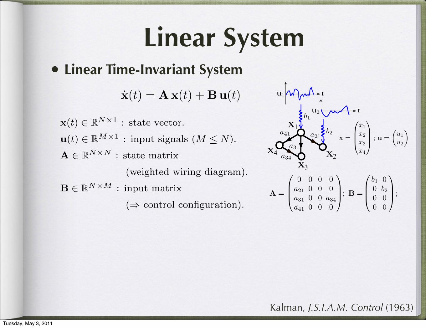
The system is stuck in a plane in the state space.
Example 2: Uncontrollable
x(t+ 1) = Ax(t) + bu(t)
⇔
x1(t+ 1)x2(t+ 1)x3(t+ 1)
=
0 0a21 0 0a31 0 0
x1(t)x2(t)x3(t)
+
b00
u(t).
⇔
x1(t+ 1) = bu(t)x2(t+ 1) = a21x1(t)x3(t+ 1) = a31x1(t)
⇒ a31x2(t+ 1)− a21x3(t+ 1) = 0 ⇒
x(t+ 1) = Ax(t) + bu(t)
⇔
x1(t+ 1)x2(t+ 1)x3(t+ 1)
=
0 0a21 0 0a31 0 0
x1(t)x2(t)x3(t)
+
b00
u(t).
⇔
x1(t+ 1) = bu(t)x2(t+ 1) = a21x1(t)x3(t+ 1) = a31x1(t)
⇒ a31x2(t+ 1)− a21x3(t+ 1) = 0 ⇒
Tuesday, May 3, 2011
!% !$
!"
#"
21 31
21
32
!"!!
The system is stuck in a plane in the state space.
Example 2: Uncontrollable
x(t+ 1) = Ax(t) + bu(t)
⇔
x1(t+ 1)x2(t+ 1)x3(t+ 1)
=
0 0a21 0 0a31 0 0
x1(t)x2(t)x3(t)
+
b00
u(t).
⇔
x1(t+ 1) = bu(t)x2(t+ 1) = a21x1(t)x3(t+ 1) = a31x1(t)
⇒ a31x2(t+ 1)− a21x3(t+ 1) = 0 ⇒
x(t+ 1) = Ax(t) + bu(t)
⇔
x1(t+ 1)x2(t+ 1)x3(t+ 1)
=
0 0a21 0 0a31 0 0
x1(t)x2(t)x3(t)
+
b00
u(t).
⇔
x1(t+ 1) = bu(t)x2(t+ 1) = a21x1(t)x3(t+ 1) = a31x1(t)
⇒ a31x2(t+ 1)− a21x3(t+ 1) = 0 ⇒
Tuesday, May 3, 2011

Questions
For an arbitrary complex network:
Tuesday, May 3, 2011

• What’s the minimum number of driver nodes (ND) ?
Questions
For an arbitrary complex network:
Tuesday, May 3, 2011

• What’s the minimum number of driver nodes (ND) ?
• How to efficiently identify them?
Questions
For an arbitrary complex network:
Tuesday, May 3, 2011

• What’s the minimum number of driver nodes (ND) ?
• How to efficiently identify them?
• Which network characteristics determine ND ?
Questions
For an arbitrary complex network:
Tuesday, May 3, 2011

Difficulties
Tuesday, May 3, 2011

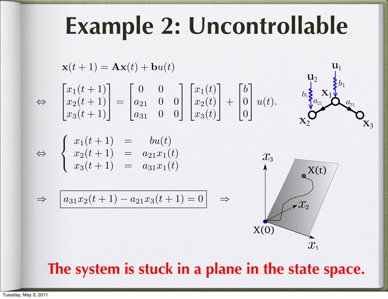
Difficulties• Parameters (link weights):
usually unknown.
!
Tuesday, May 3, 2011

Difficulties• Parameters (link weights):
usually unknown.
!
rankC = N
C = [B,AB,A2 B, · · · ,AN−1 B]
• Kalman’s rank condition:hard to check for large system(C is of dimension NxNM).
Tuesday, May 3, 2011
Difficulties• Parameters (link weights):
usually unknown.
!
�N
1
�+
�N
2
�+ · · ·+
�N
N
�= 2N − 1
rankC = N
C = [B,AB,A2 B, · · · ,AN−1 B]
• If brute-force search:(2N-1) combinations.
• Kalman’s rank condition:hard to check for large system(C is of dimension NxNM).
Tuesday, May 3, 2011

Solution
Tuesday, May 3, 2011

Solution
• Structural Controllability
• Maximum Matching
Liu et al., Nature (in press)Tuesday, May 3, 2011

IEEE TRAXSACTIONS ON AUTOMATIC CONTROL, VOL. AC-19, NO. 3, JUNE 1974 20 1
Structural Controllability CHIT\;G-TAI LIN, WENBER, IEEE
Abstract-The new concepts of “structure” and “structural con- trollability” for a linear timeinvariant control system (described by a pair ( A $ ) ) are defined and studied. The physical justification of these concepts and examples are also given.
The graph of a pair ( A $ ) is also defined. This gives another way of describing the structure of this pair. The property of structural con- trollability is reduced to a property of the graph of the pair (A,b) . To do this, the basic concept of a L‘cactus’’ and the related concept of a ‘Lprecactus” are introduced. The main result of this paper states that the pair ( A $ ) is structurally controllable if an only if the graph of (A ,b ) is “spanned by a cactus.” The result is also expressed in a more conventional way, in terms of some properties of the pair (A,b) .
I. INTRODUCTION
C ONSIDER a linear control system
x = AX + bu
with x E R”, u E R. The ma.trices A E Rnxn and b E Rn are assumed throughout to have compat.ible dimensions a.nd t.0 be time invariant. For convenience, the control system (1.1) is denoted t,hroughout. the paper by the pair (-4,b).
It is known (see Lee and Marlcus [l 1) that t.he set. of all (completely) cont,rollable pairs (1.1) is open and dense in the space of all pa.irs (A$) (with the st.andard met,ric). Thus, if the pair (Ao,bo) is not, completely controllable, t,hen for every E > 0, there exists a completely controllable pair (A$) wit,h IIA - Aoj/ < c and Ilb - bo;! < c (where I] .I) denotes norm1). This result is of an obvious physical interest. Practically, for every pair (A$), most. of the entries of A and b are known only with the approximat>ion of somr errors of measurement. Only some of t,hese ent.rirs are known with 100 percent precision. Sormally, t,his happens for some ent,ries which are equal t.0 zrros. Thus we shall assume here t,hat, there are some rntrirs of A and b which are precisely zero, while all t,he ot,hrr rntries are linowm only
We shall say that, the pair ( A $ ) has t.he same structure as another pair (A,&), of the same dimmsions, if for every fixed (zero) ent,ry of the matrix (Ab), tjhe corresponding entry of the matrix (Ab) is fixed (zero) and, at t,he samr t,imc, for every fixed (zero) entrl- of (rig), the correspond-
hranuscript. received Kovember 15, 1972; revised August, 16, 1973. Paper reconmended by A. Stephen Morse, Chairman of IEEE S-CS Linear Systems Commit,tee.
The author was with t.he Department of Electrical Engineering and Electronics Laboratory, Universit.y of Xaryland, College Pa.rk,
tion, Columbia, Md. 21043. Md. 20742. He is now nit.h t.he Bendis Field Engineering Corpora-
1 For inst.ance, if ai j and bi are the ent,ries of A and b, respec- t,ively, thenwemaytake l l A l l ; , ~ = 1 , . . . , n = maxlaijl and i!bl\ i=l. . . . ,n = max Ibil.
2 Other possible assumptions are left for furt.her research.
ing entry of (Ab) is also fixed (zero). Then one defines the pair @,,bo) to be structurally controllable if a.nd only if there exists a completely controllable pair (A$) which has the same structure as (&,bo).
The concept of “st.ruct,ural cont.rollabilitf’ of a pair ( A & ) makes the mcaning of controllability (in the usual sense) more complete from the physical point of view. In fact, itt is preferred whenever (Ao,bo) represents an actual physical system (that. involves parameters only approximat.cly det.ermined). Actually, thc completely cont.rolla.ble pair (A$) can be considered as “physically undistinguishable” from the pair (,4,,bo) (sce the following proposition). From this viewpoint, the concept of struc- tural cont,rollabilit,y has a physical justification. Indeed, the definition of st.ruct,ural cont.rollability is equivalent to a st,rongcr property as shown by the following proposition.
Propositim2 1: The pair (Ao,bo) is structurally contxollable if and only if ‘OLE > 0, there cxist,s a completely cont.rollablc pair (A1,bl) of the same struct,ure as (Ao,bo) such that ~ I A I - A n ] / < c a.nd llbl - bo;: < e .
Indrrd, if the pr0pert.y in Proposition 1 is sat,isfied, then thc pair (AO&) is obviously structurally controllable. Conversely, assume now t,hat t.he pair (Ao,bo) is st,ruc- turally controllable, i.c., there exist.s a completely con- trollable pair (A2,b2) of the same structure as (Ao,bo). Consider now t,he pairs, A(X) = (1 - X)& + XAS; b(X) = (1 - X)bo + Abs, where hc[0,1]. Then #(X) = det @(X) A(X)b(X), -4(X)”-%(X)) is a polynomial in X, and this poly- nomial is not. identically zero (since it is diff erent from zero for X = 1). Clearly, given an arbitrary > 0, one can find X 0 ~ [ 0 , 1 ] such t,hat ~ \ A ( x ) - A o l l < e and Ilb(X) - bdj < ~ , ‘ ~ X X E [ O , X ~ ] . Furt.her one can find Xlc[O,ho] such that, #(XI) # 0, Le., t>he pair (A(hl),b(Xl)) is complrtely con- trollablc--and onc has obt.ained t.hc property in Proposi- tion 1. Q.E.D.
It, is immediate that, cvery completely controllable pa.ir (A$) is also structurally controllable. Rlorrover, if no entry of (A$) is fixed, then tlhe pair (A$) is struct,urally controllable (t.his also follows from the LeeMarkus result ment,ioned in the introduction). However, if some cnt,ries of ( A $ ) are fixed, the pa.ir ma,y not be structurally con- trollablr. Consider, for inst.ancc, the pair (A$) of the form
\~11erc All E R P X k , A P 1 E R ( ” - k ) X k > L4 22 E R( ” -p )X(n - - l i )
b2 E R“-k((l 5 h- 5 , I ) , ) , and by 0, onc denotes a matrix or a vector containing only fixed (zero) entries. Then, i t is easy to ser tha.t, rank (b-46. . .A”-%) is less than n. (indc pendently of the valurs of All , A s l , Az, and b2). Thus the pair (1.2) is not structurally controllable.
Authorized licensed use limited to: University of Illinois. Downloaded on November 11, 2009 at 15:38 from IEEE Xplore. Restrictions apply.
208 IEEE TRANSACTIONS ON AUT031.4TIC CONTROL, JUNE 1974
dimension can be partitioned into two sets: The set. of the pairs ( A $ ) , which are not. structurally controllable, and the set. of t,he pairs (A$) , which are structurally con- trollable. We also gave several necessarv and sufficient. condit,ions of structural controllabilit,y. Thc introduction of t.he structurally controllable set is justified by the remark that, taking into account, the presence of the errors of measurements, we cannot decide, by physical measure- ments, whether or not, a pair (A$) is completely con- trollable or only structurally controllable. For instancc, consider t.he circuit shown in Fig. 6, in which u is the input. volt,age and y is the out,put current. It is a sinple- input singlcout.put system. Let. the voltagcl arrow the capacitor and thc current flowing through the inductor bn the 5ta.tevariables TI and x?, respectively [*I. Then the system can be ea,sily described as .i = A . E + bu, (den0tc.d by t he pair ( A ? b ) ) , where
Suppose t,hc components of the circuit, R1, R?. C, and I,, have unit. values? a.nd let. @,.bo) be the pair with these specified values in the entries of ( A $ ) . Then the pair
pair (Ao&) is not complet.ely controllablr since rank (bo A&,) < 2. However, by the definit,ion of structural con- t,rollability or the theorem in this section, one sees that the pairs (A$) and (&,bo), having the same structure, are both structurally cont,rollable.
The study of the structure and the graph of a pair (A$) (1.1) in this work results in a more precise controllability property in the cont.rol s?-stem. Furthermorc, it will also be possible to derive some basic properties in matrix and graph theories. For instancc? by mamining the theorem in this yection, structural controllability cquiv:d(wcc condi- tions could be related to the irreducibility properties in matrix throry, ergodic propcrt,ies of IIarkov chains, nnd the iden of thr shortest length in graph thcory. 3Iorcover. the control q-stem (1.1) studied here has a single input and is time invariant. It is left for further research to establish results like the theorrm in Section 1’ for thc multi-input and timcvariant cases. I t would bn also in- t.eresting to study the dual property of drurturnl observ-
ability of a l inea observed system. Thus the c0ncept.s of “structure” and “struct,ural controllabilit,y” a.nd t,he results obta,ined here are only the first step in what, is believed to bo a promising new branch in control system theory.
ACKNOWLEDGMENT The aut,hor Tlishes to express his grat.itudc to Prof.
V. 31. Popov of thr University of hlaryland for his sugges- tion and guidance in the course of this rrwarch.
REFEREWES E. B. Lee and L. Markus, F o u n d d i m of Optimal Control Theory. New York: Wiley, 1967. 0. Ore, “Theory of Graphs,” Anzer. Math. SOC. Col1oquiu.m Publ., vol. 38, 1962. V. 11. Popov, Hyperstmi1itate.s sistemlor autmnaje (in Ronla- nian). Sew York: Springer, to he published. L. A. Zadeh and C. 4 . Deoer, Linear Sgsfem Theory. Sew York: JIcGraw-Hill, 1963. F. R. Gant,macher, The Theory of Xdrices. h-ew York: vol. 1 and 2, Chelsea Publkhing Campany, 1960. It. E. KF!man, “1Iathematical description of linear dynamical s;vstenls, S Z A X J . Cont~., vol. 1, 1963. It. W . Brocket.t, Finite Dimensional Linear Systems. New York: Wiley, 19’70. K. S. Varga, Slairix Ikrutive Analysis. Engleaood Cliffs, K.J.: Prent.ice-Hall, 1962. J . G. Kemeny and J. L. Snell, Finiie -1farRm: Chains. Prince- ton, K. J.: Van Sost,rand, 1960. I) . G. Luenberger, “Canonical forms for linear mult.ivariable systems,” IEEE Trans. Auto. Conir., June 1967. IXnw Kiinig, Theories der Endlichen m d c.’nend/ichen Graphen. Kea Tork: Chelsea Publishing Company, 19.70. C. T. Lin, “Struct.ura1 controllability,’‘ Ph.1). dissert.ation, Dep. Elec. Eng., Univ. of lIar?;land, College Park, Md., 19’72.
Ching-Tai Lin (S’73-31’73) m-as born in Taipei, China, on October 14, 10-%4. He re- ceived the B.S. degree in electrical engineering from Kational Taiwan Gnivewit.y, Taipei, Taiwan, China in 196’7, and the 313. and Ph.1). degrees in electrical engineering from the University of JIaryland, College Park, JId. in 1970 and 1972, respectively.
From 1967 tu 1966, he wCas a Second Lientenant Electronia Officer in the Chinese Air Force, Taiwan, China. He m-a? a Research
Assistant end a Tenching Assistant at t.he Electronics Research Laboratory, Fnivenity of 3Iaryland during 1065-1069 and 1069- 1972, respectivelv. I n 1973, he, as an Instructor, taught at the Electrical Engineering Depart.ment, Howard Cniversity, Washing- ton, D.C. Since Jmne 1973. he has been with Bendis Field Engineering Corp.. Columbia, 3rd. where he is now a Senior System Engineer. His current. rvsearch interests include linear system theory and process control, and stability theory.
Authorized licensed use limited to: University of Illinois. Downloaded on November 11, 2009 at 15:38 from IEEE Xplore. Restrictions apply.
Lin, IEEE Trans. Auto. Contr. (1974)Tuesday, May 3, 2011

Structural Controllability
Tuesday, May 3, 2011

Structural Controllability
!$!%
!#
!&
"&"#
!$!%
!#
!&
"&"#
!$!%
!#
!&
"&"#
· · ·· · ·
Tuesday, May 3, 2011

Structural Controllability
!$!%
!#
!&
"&"#
� �� �!$
!%!#
!&
"&"#
!$!%
!#
!&
"&"#
!$!%
!#
!&
"&"#
· · ·· · ·
Tuesday, May 3, 2011

Structural Controllability
!$!%
!#
!&
"&"#
� �� �
Structured Matrix: Its elements are either fixed zeros or independent free parameters.
!$!%
!#
!&
"&"#
!$!%
!#
!&
"&"#
!$!%
!#
!&
"&"#
· · ·· · ·
Tuesday, May 3, 2011

Structural Controllability
!$!%
!#
!&
"&"#
� �� �
Structured Matrix: Its elements are either fixed zeros or independent free parameters.
Only the structure matters!
!$!%
!#
!&
"&"#
!$!%
!#
!&
"&"#
!$!%
!#
!&
"&"#
· · ·· · ·
Tuesday, May 3, 2011

4
31
23
21
23
a b c d
21 31
21
32
x2
x3x1
u1
21 31
33
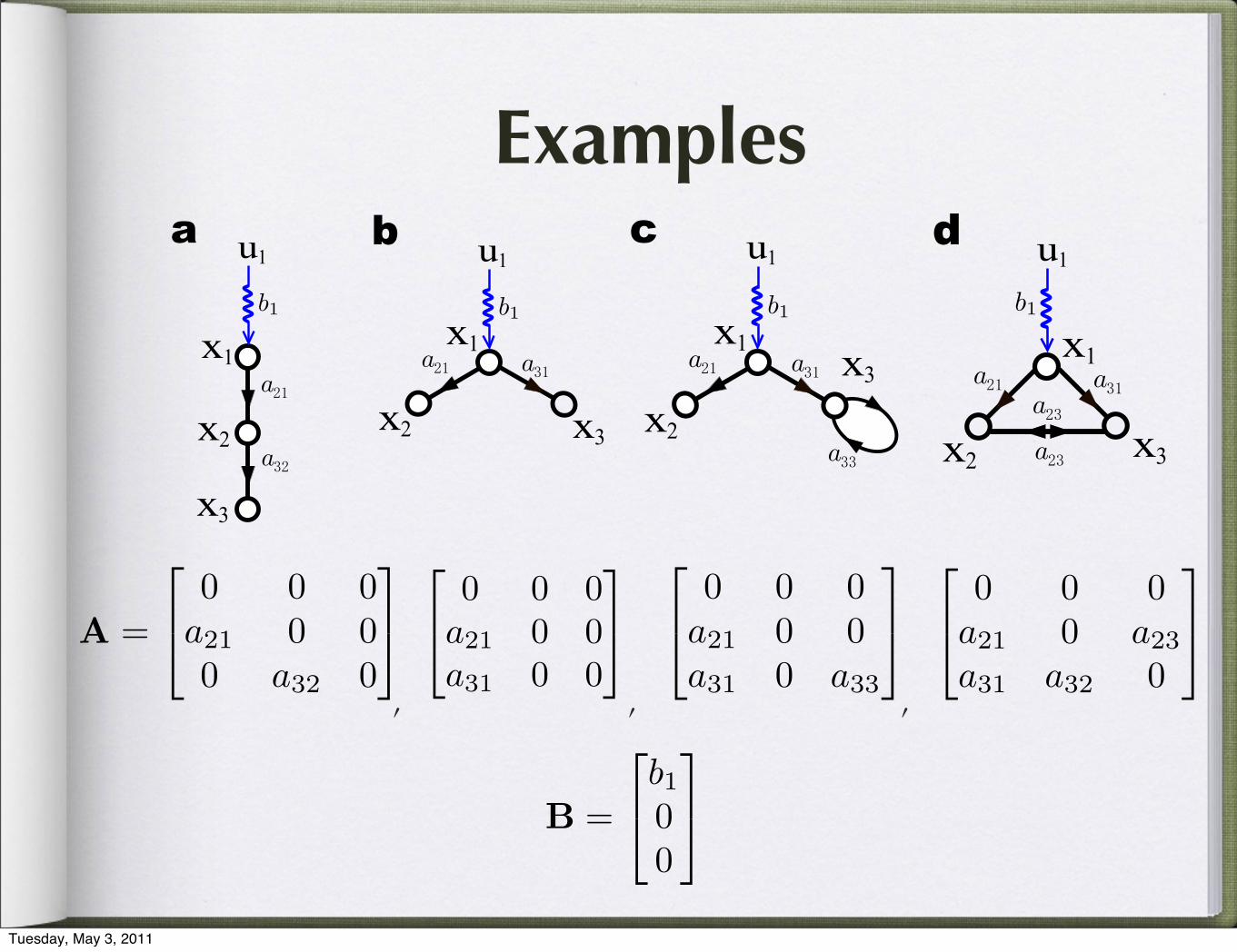
Figure S1: Control simple networks. a, A directed path can be completely controlled by controlling the
starting node only. The controllability is independent of the detailed (non-zero) values of b1, a21, and a32,
so the system is strongly structurally controllable. b, A directed star can never be completely controlled by
controlling the central hub (node x1) only. c, This example network, generated by adding a self-edge to the
star shown in b, can be completely controlled by controlling node x1 only. The controllability is independent
of the detailed (non-zero) values of b1, a21, a31, and a33, so the system is strongly structurally controllable.
d, This network is completely controllable for almost all weights combinations. It will be uncontrollable
only in some pathological cases, e.g. those weights satisfy the constraint a32a221 = a23a2
31 exactly, so the
system is structurally controllable.
The controllability matrix is given by
C = [B,A · B,A2 · B] = b1
1 0 0
0 a21 0
0 0 a32a21
.
Since rankC = 3 = N , so the system is controllable. Note that the system is always controllable
as long as those weights, i.e. a21, a32 and b1, are non-zero. In other words, its controllability is
independent of the detailed values of a21, a32 and b1. This is an example of the so called strong
structural controllability [3].
The linear dynamics shown in Fig. S1(b) can be written as
x1(t)
x2(t)
x3(t)
=
0 0 0
a21 0 0
a31 0 0
·
x1(t)
x2(t)
x3(t)
+
b1
0
0
u(t).
4
31
23
21
23
a b c d
x2 x3
x1
u1
21 31
21
32
21 31
33
Figure S1: Control simple networks. a, A directed path can be completely controlled by controlling the
starting node only. The controllability is independent of the detailed (non-zero) values of b1, a21, and a32,
so the system is strongly structurally controllable. b, A directed star can never be completely controlled by
controlling the central hub (node x1) only. c, This example network, generated by adding a self-edge to the
star shown in b, can be completely controlled by controlling node x1 only. The controllability is independent
of the detailed (non-zero) values of b1, a21, a31, and a33, so the system is strongly structurally controllable.
d, This network is completely controllable for almost all weights combinations. It will be uncontrollable
only in some pathological cases, e.g. those weights satisfy the constraint a32a221 = a23a2
31 exactly, so the
system is structurally controllable.
The controllability matrix is given by
C = [B,A · B,A2 · B] = b1
1 0 0
0 a21 0
0 0 a32a21
.
Since rankC = 3 = N , so the system is controllable. Note that the system is always controllable
as long as those weights, i.e. a21, a32 and b1, are non-zero. In other words, its controllability is
independent of the detailed values of a21, a32 and b1. This is an example of the so called strong
structural controllability [3].
The linear dynamics shown in Fig. S1(b) can be written as
x1(t)
x2(t)
x3(t)
=
0 0 0
a21 0 0
a31 0 0
·
x1(t)
x2(t)
x3(t)
+
b1
0
0
u(t).
4
31
23
21
23
a b c d
21 31x1
x2
x3
u1
21
32
21 31
33
Figure S1: Control simple networks. a, A directed path can be completely controlled by controlling the
starting node only. The controllability is independent of the detailed (non-zero) values of b1, a21, and a32,
so the system is strongly structurally controllable. b, A directed star can never be completely controlled by
controlling the central hub (node x1) only. c, This example network, generated by adding a self-edge to the
star shown in b, can be completely controlled by controlling node x1 only. The controllability is independent
of the detailed (non-zero) values of b1, a21, a31, and a33, so the system is strongly structurally controllable.
d, This network is completely controllable for almost all weights combinations. It will be uncontrollable
only in some pathological cases, e.g. those weights satisfy the constraint a32a221 = a23a2
31 exactly, so the
system is structurally controllable.
The controllability matrix is given by
C = [B,A · B,A2 · B] = b1
1 0 0
0 a21 0
0 0 a32a21
.
Since rankC = 3 = N , so the system is controllable. Note that the system is always controllable
as long as those weights, i.e. a21, a32 and b1, are non-zero. In other words, its controllability is
independent of the detailed values of a21, a32 and b1. This is an example of the so called strong
structural controllability [3].
The linear dynamics shown in Fig. S1(b) can be written as
x1(t)
x2(t)
x3(t)
=
0 0 0
a21 0 0
a31 0 0
·
x1(t)
x2(t)
x3(t)
+
b1
0
0
u(t).
4
x3x2
x131
23
21
23
u1a b c d
21 31
21
32
21 31
33
Figure S1: Control simple networks. a, A directed path can be completely controlled by controlling the
starting node only. The controllability is independent of the detailed (non-zero) values of b1, a21, and a32,
so the system is strongly structurally controllable. b, A directed star can never be completely controlled by
controlling the central hub (node x1) only. c, This example network, generated by adding a self-edge to the
star shown in b, can be completely controlled by controlling node x1 only. The controllability is independent
of the detailed (non-zero) values of b1, a21, a31, and a33, so the system is strongly structurally controllable.
d, This network is completely controllable for almost all weights combinations. It will be uncontrollable
only in some pathological cases, e.g. those weights satisfy the constraint a32a221 = a23a2
31 exactly, so the
system is structurally controllable.
The controllability matrix is given by
C = [B,A · B,A2 · B] = b1
1 0 0
0 a21 0
0 0 a32a21
.
Since rankC = 3 = N , so the system is controllable. Note that the system is always controllable
as long as those weights, i.e. a21, a32 and b1, are non-zero. In other words, its controllability is
independent of the detailed values of a21, a32 and b1. This is an example of the so called strong
structural controllability [3].
The linear dynamics shown in Fig. S1(b) can be written as
x1(t)
x2(t)
x3(t)
=
0 0 0
a21 0 0
a31 0 0
·
x1(t)
x2(t)
x3(t)
+
b1
0
0
u(t).
Examples
Tuesday, May 3, 2011

4
31
23
21
23
a b c d
21 31
21
32
x2
x3x1
u1
21 31
33
Figure S1: Control simple networks. a, A directed path can be completely controlled by controlling the
starting node only. The controllability is independent of the detailed (non-zero) values of b1, a21, and a32,
so the system is strongly structurally controllable. b, A directed star can never be completely controlled by
controlling the central hub (node x1) only. c, This example network, generated by adding a self-edge to the
star shown in b, can be completely controlled by controlling node x1 only. The controllability is independent
of the detailed (non-zero) values of b1, a21, a31, and a33, so the system is strongly structurally controllable.
d, This network is completely controllable for almost all weights combinations. It will be uncontrollable
only in some pathological cases, e.g. those weights satisfy the constraint a32a221 = a23a2
31 exactly, so the
system is structurally controllable.
The controllability matrix is given by
C = [B,A · B,A2 · B] = b1
1 0 0
0 a21 0
0 0 a32a21
.
Since rankC = 3 = N , so the system is controllable. Note that the system is always controllable
as long as those weights, i.e. a21, a32 and b1, are non-zero. In other words, its controllability is
independent of the detailed values of a21, a32 and b1. This is an example of the so called strong
structural controllability [3].
The linear dynamics shown in Fig. S1(b) can be written as
x1(t)
x2(t)
x3(t)
=
0 0 0
a21 0 0
a31 0 0
·
x1(t)
x2(t)
x3(t)
+
b1
0
0
u(t).
4
31
23
21
23
a b c d
x2 x3
x1
u1
21 31
21
32
21 31
33
Figure S1: Control simple networks. a, A directed path can be completely controlled by controlling the
starting node only. The controllability is independent of the detailed (non-zero) values of b1, a21, and a32,
so the system is strongly structurally controllable. b, A directed star can never be completely controlled by
controlling the central hub (node x1) only. c, This example network, generated by adding a self-edge to the
star shown in b, can be completely controlled by controlling node x1 only. The controllability is independent
of the detailed (non-zero) values of b1, a21, a31, and a33, so the system is strongly structurally controllable.
d, This network is completely controllable for almost all weights combinations. It will be uncontrollable
only in some pathological cases, e.g. those weights satisfy the constraint a32a221 = a23a2
31 exactly, so the
system is structurally controllable.
The controllability matrix is given by
C = [B,A · B,A2 · B] = b1
1 0 0
0 a21 0
0 0 a32a21
.
Since rankC = 3 = N , so the system is controllable. Note that the system is always controllable
as long as those weights, i.e. a21, a32 and b1, are non-zero. In other words, its controllability is
independent of the detailed values of a21, a32 and b1. This is an example of the so called strong
structural controllability [3].
The linear dynamics shown in Fig. S1(b) can be written as
x1(t)
x2(t)
x3(t)
=
0 0 0
a21 0 0
a31 0 0
·
x1(t)
x2(t)
x3(t)
+
b1
0
0
u(t).
4
31
23
21
23
a b c d
21 31x1
x2
x3
u1
21
32
21 31
33
Figure S1: Control simple networks. a, A directed path can be completely controlled by controlling the
starting node only. The controllability is independent of the detailed (non-zero) values of b1, a21, and a32,
so the system is strongly structurally controllable. b, A directed star can never be completely controlled by
controlling the central hub (node x1) only. c, This example network, generated by adding a self-edge to the
star shown in b, can be completely controlled by controlling node x1 only. The controllability is independent
of the detailed (non-zero) values of b1, a21, a31, and a33, so the system is strongly structurally controllable.
d, This network is completely controllable for almost all weights combinations. It will be uncontrollable
only in some pathological cases, e.g. those weights satisfy the constraint a32a221 = a23a2
31 exactly, so the
system is structurally controllable.
The controllability matrix is given by
C = [B,A · B,A2 · B] = b1
1 0 0
0 a21 0
0 0 a32a21
.
Since rankC = 3 = N , so the system is controllable. Note that the system is always controllable
as long as those weights, i.e. a21, a32 and b1, are non-zero. In other words, its controllability is
independent of the detailed values of a21, a32 and b1. This is an example of the so called strong
structural controllability [3].
The linear dynamics shown in Fig. S1(b) can be written as
x1(t)
x2(t)
x3(t)
=
0 0 0
a21 0 0
a31 0 0
·
x1(t)
x2(t)
x3(t)
+
b1
0
0
u(t).
4
x3x2
x131
23
21
23
u1a b c d
21 31
21
32
21 31
33
Figure S1: Control simple networks. a, A directed path can be completely controlled by controlling the
starting node only. The controllability is independent of the detailed (non-zero) values of b1, a21, and a32,
so the system is strongly structurally controllable. b, A directed star can never be completely controlled by
controlling the central hub (node x1) only. c, This example network, generated by adding a self-edge to the
star shown in b, can be completely controlled by controlling node x1 only. The controllability is independent
of the detailed (non-zero) values of b1, a21, a31, and a33, so the system is strongly structurally controllable.
d, This network is completely controllable for almost all weights combinations. It will be uncontrollable
only in some pathological cases, e.g. those weights satisfy the constraint a32a221 = a23a2
31 exactly, so the
system is structurally controllable.
The controllability matrix is given by
C = [B,A · B,A2 · B] = b1
1 0 0
0 a21 0
0 0 a32a21
.
Since rankC = 3 = N , so the system is controllable. Note that the system is always controllable
as long as those weights, i.e. a21, a32 and b1, are non-zero. In other words, its controllability is
independent of the detailed values of a21, a32 and b1. This is an example of the so called strong
structural controllability [3].
The linear dynamics shown in Fig. S1(b) can be written as
x1(t)
x2(t)
x3(t)
=
0 0 0
a21 0 0
a31 0 0
·
x1(t)
x2(t)
x3(t)
+
b1
0
0
u(t).
Examples
0 0 0a21 0 0a31 0 0
0 0 0a21 0 0a31 0 a33
0 0 0a21 0 a23a31 a32 0
A =
0 0 0a21 0 00 a32 0
, , ,
Tuesday, May 3, 2011
4
31
23
21
23
a b c d
21 31
21
32
x2
x3x1
u1
21 31
33
Figure S1: Control simple networks. a, A directed path can be completely controlled by controlling the
starting node only. The controllability is independent of the detailed (non-zero) values of b1, a21, and a32,
so the system is strongly structurally controllable. b, A directed star can never be completely controlled by
controlling the central hub (node x1) only. c, This example network, generated by adding a self-edge to the
star shown in b, can be completely controlled by controlling node x1 only. The controllability is independent
of the detailed (non-zero) values of b1, a21, a31, and a33, so the system is strongly structurally controllable.
d, This network is completely controllable for almost all weights combinations. It will be uncontrollable
only in some pathological cases, e.g. those weights satisfy the constraint a32a221 = a23a2
31 exactly, so the
system is structurally controllable.
The controllability matrix is given by
C = [B,A · B,A2 · B] = b1
1 0 0
0 a21 0
0 0 a32a21
.
Since rankC = 3 = N , so the system is controllable. Note that the system is always controllable
as long as those weights, i.e. a21, a32 and b1, are non-zero. In other words, its controllability is
independent of the detailed values of a21, a32 and b1. This is an example of the so called strong
structural controllability [3].
The linear dynamics shown in Fig. S1(b) can be written as
x1(t)
x2(t)
x3(t)
=
0 0 0
a21 0 0
a31 0 0
·
x1(t)
x2(t)
x3(t)
+
b1
0
0
u(t).
4
31
23
21
23
a b c d
x2 x3
x1
u1
21 31
21
32
21 31
33
Figure S1: Control simple networks. a, A directed path can be completely controlled by controlling the
starting node only. The controllability is independent of the detailed (non-zero) values of b1, a21, and a32,
so the system is strongly structurally controllable. b, A directed star can never be completely controlled by
controlling the central hub (node x1) only. c, This example network, generated by adding a self-edge to the
star shown in b, can be completely controlled by controlling node x1 only. The controllability is independent
of the detailed (non-zero) values of b1, a21, a31, and a33, so the system is strongly structurally controllable.
d, This network is completely controllable for almost all weights combinations. It will be uncontrollable
only in some pathological cases, e.g. those weights satisfy the constraint a32a221 = a23a2
31 exactly, so the
system is structurally controllable.
The controllability matrix is given by
C = [B,A · B,A2 · B] = b1
1 0 0
0 a21 0
0 0 a32a21
.
Since rankC = 3 = N , so the system is controllable. Note that the system is always controllable
as long as those weights, i.e. a21, a32 and b1, are non-zero. In other words, its controllability is
independent of the detailed values of a21, a32 and b1. This is an example of the so called strong
structural controllability [3].
The linear dynamics shown in Fig. S1(b) can be written as
x1(t)
x2(t)
x3(t)
=
0 0 0
a21 0 0
a31 0 0
·
x1(t)
x2(t)
x3(t)
+
b1
0
0
u(t).
4
31
23
21
23
a b c d
21 31x1
x2
x3
u1
21
32
21 31
33
Figure S1: Control simple networks. a, A directed path can be completely controlled by controlling the
starting node only. The controllability is independent of the detailed (non-zero) values of b1, a21, and a32,
so the system is strongly structurally controllable. b, A directed star can never be completely controlled by
controlling the central hub (node x1) only. c, This example network, generated by adding a self-edge to the
star shown in b, can be completely controlled by controlling node x1 only. The controllability is independent
of the detailed (non-zero) values of b1, a21, a31, and a33, so the system is strongly structurally controllable.
d, This network is completely controllable for almost all weights combinations. It will be uncontrollable
only in some pathological cases, e.g. those weights satisfy the constraint a32a221 = a23a2
31 exactly, so the
system is structurally controllable.
The controllability matrix is given by
C = [B,A · B,A2 · B] = b1
1 0 0
0 a21 0
0 0 a32a21
.
Since rankC = 3 = N , so the system is controllable. Note that the system is always controllable
as long as those weights, i.e. a21, a32 and b1, are non-zero. In other words, its controllability is
independent of the detailed values of a21, a32 and b1. This is an example of the so called strong
structural controllability [3].
The linear dynamics shown in Fig. S1(b) can be written as
x1(t)
x2(t)
x3(t)
=
0 0 0
a21 0 0
a31 0 0
·
x1(t)
x2(t)
x3(t)
+
b1
0
0
u(t).
4
x3x2
x131
23
21
23
u1a b c d
21 31
21
32
21 31
33
Figure S1: Control simple networks. a, A directed path can be completely controlled by controlling the
starting node only. The controllability is independent of the detailed (non-zero) values of b1, a21, and a32,
so the system is strongly structurally controllable. b, A directed star can never be completely controlled by
controlling the central hub (node x1) only. c, This example network, generated by adding a self-edge to the
star shown in b, can be completely controlled by controlling node x1 only. The controllability is independent
of the detailed (non-zero) values of b1, a21, a31, and a33, so the system is strongly structurally controllable.
d, This network is completely controllable for almost all weights combinations. It will be uncontrollable
only in some pathological cases, e.g. those weights satisfy the constraint a32a221 = a23a2
31 exactly, so the
system is structurally controllable.
The controllability matrix is given by
C = [B,A · B,A2 · B] = b1
1 0 0
0 a21 0
0 0 a32a21
.
Since rankC = 3 = N , so the system is controllable. Note that the system is always controllable
as long as those weights, i.e. a21, a32 and b1, are non-zero. In other words, its controllability is
independent of the detailed values of a21, a32 and b1. This is an example of the so called strong
structural controllability [3].
The linear dynamics shown in Fig. S1(b) can be written as
x1(t)
x2(t)
x3(t)
=
0 0 0
a21 0 0
a31 0 0
·
x1(t)
x2(t)
x3(t)
+
b1
0
0
u(t).
Examples
0 0 0a21 0 0a31 0 0
0 0 0a21 0 0a31 0 a33
0 0 0a21 0 a23a31 a32 0
A =
0 0 0a21 0 00 a32 0
, , ,
B =
b100
Tuesday, May 3, 2011

4
31
23
21
23
a b c d
21 31
21
32
x2
x3x1
u1
21 31
33
Figure S1: Control simple networks. a, A directed path can be completely controlled by controlling the
starting node only. The controllability is independent of the detailed (non-zero) values of b1, a21, and a32,
so the system is strongly structurally controllable. b, A directed star can never be completely controlled by
controlling the central hub (node x1) only. c, This example network, generated by adding a self-edge to the
star shown in b, can be completely controlled by controlling node x1 only. The controllability is independent
of the detailed (non-zero) values of b1, a21, a31, and a33, so the system is strongly structurally controllable.
d, This network is completely controllable for almost all weights combinations. It will be uncontrollable
only in some pathological cases, e.g. those weights satisfy the constraint a32a221 = a23a2
31 exactly, so the
system is structurally controllable.
The controllability matrix is given by
C = [B,A · B,A2 · B] = b1
1 0 0
0 a21 0
0 0 a32a21
.
Since rankC = 3 = N , so the system is controllable. Note that the system is always controllable
as long as those weights, i.e. a21, a32 and b1, are non-zero. In other words, its controllability is
independent of the detailed values of a21, a32 and b1. This is an example of the so called strong
structural controllability [3].
The linear dynamics shown in Fig. S1(b) can be written as
x1(t)
x2(t)
x3(t)
=
0 0 0
a21 0 0
a31 0 0
·
x1(t)
x2(t)
x3(t)
+
b1
0
0
u(t).
4
31
23
21
23
a b c d
x2 x3
x1
u1
21 31
21
32
21 31
33
Figure S1: Control simple networks. a, A directed path can be completely controlled by controlling the
starting node only. The controllability is independent of the detailed (non-zero) values of b1, a21, and a32,
so the system is strongly structurally controllable. b, A directed star can never be completely controlled by
controlling the central hub (node x1) only. c, This example network, generated by adding a self-edge to the
star shown in b, can be completely controlled by controlling node x1 only. The controllability is independent
of the detailed (non-zero) values of b1, a21, a31, and a33, so the system is strongly structurally controllable.
d, This network is completely controllable for almost all weights combinations. It will be uncontrollable
only in some pathological cases, e.g. those weights satisfy the constraint a32a221 = a23a2
31 exactly, so the
system is structurally controllable.
The controllability matrix is given by
C = [B,A · B,A2 · B] = b1
1 0 0
0 a21 0
0 0 a32a21
.
Since rankC = 3 = N , so the system is controllable. Note that the system is always controllable
as long as those weights, i.e. a21, a32 and b1, are non-zero. In other words, its controllability is
independent of the detailed values of a21, a32 and b1. This is an example of the so called strong
structural controllability [3].
The linear dynamics shown in Fig. S1(b) can be written as
x1(t)
x2(t)
x3(t)
=
0 0 0
a21 0 0
a31 0 0
·
x1(t)
x2(t)
x3(t)
+
b1
0
0
u(t).
4
31
23
21
23
a b c d
21 31x1
x2
x3
u1
21
32
21 31
33
Figure S1: Control simple networks. a, A directed path can be completely controlled by controlling the
starting node only. The controllability is independent of the detailed (non-zero) values of b1, a21, and a32,
so the system is strongly structurally controllable. b, A directed star can never be completely controlled by
controlling the central hub (node x1) only. c, This example network, generated by adding a self-edge to the
star shown in b, can be completely controlled by controlling node x1 only. The controllability is independent
of the detailed (non-zero) values of b1, a21, a31, and a33, so the system is strongly structurally controllable.
d, This network is completely controllable for almost all weights combinations. It will be uncontrollable
only in some pathological cases, e.g. those weights satisfy the constraint a32a221 = a23a2
31 exactly, so the
system is structurally controllable.
The controllability matrix is given by
C = [B,A · B,A2 · B] = b1
1 0 0
0 a21 0
0 0 a32a21
.
Since rankC = 3 = N , so the system is controllable. Note that the system is always controllable
as long as those weights, i.e. a21, a32 and b1, are non-zero. In other words, its controllability is
independent of the detailed values of a21, a32 and b1. This is an example of the so called strong
structural controllability [3].
The linear dynamics shown in Fig. S1(b) can be written as
x1(t)
x2(t)
x3(t)
=
0 0 0
a21 0 0
a31 0 0
·
x1(t)
x2(t)
x3(t)
+
b1
0
0
u(t).
4
x3x2
x131
23
21
23
u1a b c d
21 31
21
32
21 31
33
Figure S1: Control simple networks. a, A directed path can be completely controlled by controlling the
starting node only. The controllability is independent of the detailed (non-zero) values of b1, a21, and a32,
so the system is strongly structurally controllable. b, A directed star can never be completely controlled by
controlling the central hub (node x1) only. c, This example network, generated by adding a self-edge to the
star shown in b, can be completely controlled by controlling node x1 only. The controllability is independent
of the detailed (non-zero) values of b1, a21, a31, and a33, so the system is strongly structurally controllable.
d, This network is completely controllable for almost all weights combinations. It will be uncontrollable
only in some pathological cases, e.g. those weights satisfy the constraint a32a221 = a23a2
31 exactly, so the
system is structurally controllable.
The controllability matrix is given by
C = [B,A · B,A2 · B] = b1
1 0 0
0 a21 0
0 0 a32a21
.
Since rankC = 3 = N , so the system is controllable. Note that the system is always controllable
as long as those weights, i.e. a21, a32 and b1, are non-zero. In other words, its controllability is
independent of the detailed values of a21, a32 and b1. This is an example of the so called strong
structural controllability [3].
The linear dynamics shown in Fig. S1(b) can be written as
x1(t)
x2(t)
x3(t)
=
0 0 0
a21 0 0
a31 0 0
·
x1(t)
x2(t)
x3(t)
+
b1
0
0
u(t).
Examples
C = [B,A ·B,A2 ·B]
Tuesday, May 3, 2011

4
31
23
21
23
a b c d
21 31
21
32
21 31
33
Figure S1: Control simple networks. a, A directed path can be completely controlled by controlling the
starting node only. The controllability is independent of the detailed (non-zero) values of b1, a21, and a32,
so the system is strongly structurally controllable. b, A directed star can never be completely controlled by
controlling the central hub (node x1) only. c, This example network, generated by adding a self-edge to the
star shown in b, can be completely controlled by controlling node x1 only. The controllability is independent
of the detailed (non-zero) values of b1, a21, a31, and a33, so the system is strongly structurally controllable.
d, This network is completely controllable for almost all weights combinations. It will be uncontrollable
only in some pathological cases, e.g. those weights satisfy the constraint a32a221 = a23a2
31 exactly, so the
system is structurally controllable.
The controllability matrix is given by
C = [B,A · B,A2 · B] = b1
1 0 0
0 a21 0
0 0 a32a21
.
Since rankC = 3 = N , so the system is controllable. Note that the system is always controllable
as long as those weights, i.e. a21, a32 and b1, are non-zero. In other words, its controllability is
independent of the detailed values of a21, a32 and b1. This is an example of the so called strong
structural controllability [3].
The linear dynamics shown in Fig. S1(b) can be written as
x1(t)
x2(t)
x3(t)
=
0 0 0
a21 0 0
a31 0 0
·
x1(t)
x2(t)
x3(t)
+
b1
0
0
u(t).
5
The controllability matrix is given by
C = [B,A · B,A2 · B] = b1
1 0 0
0 a21 0
0 a31 0
.
Since rankC = 2 < N , so the system is uncontrollable. Note that this is independent of the detailed
values of a21, a31, and b1. No matter how we tune them, the system is not controllable. Indeed,
the dynamics equation suggest that the system will get stuck on the plane : a31x2(t) = a21x3(t) in
the state space.
The linear dynamics shown in Fig. S1(c) can be written as
x1(t)
x2(t)
x3(t)
=
0 0 0
a21 0 0
a31 0 a33
·
x1(t)
x2(t)
x3(t)
+
b1
0
0
u(t).
The controllability matrix is given by
C = [B,A · B,A2 · B] = b1
1 0 0
0 a21 0
0 a31 a33a31
.
Since rankC = 3 = N , so the system is controllable. In this example, the controllability is
independent of the detailed values of a21, a31 , a33, and b1, as long as they are non-zero. This
is another example of strong structural controllability. Notice the small difference between the
networks shown in Fig. S1(b) and Fig. S1(c). The presence of a self-edge fundamentally changes
the controllability of the system.
The linear dynamics shown in Fig. S1(d) can be written as
x1(t)
x2(t)
x3(t)
=
0 0 0
a21 0 a23
a31 a32 0
·
x1(t)
x2(t)
x3(t)
+
b1
0
0
u(t).
The controllability matrix can be easily calculated
C = [B,A · B,A2 · B] = b1
1 0 0
0 a21 a23a31
0 a31 a32a21
.
In most cases, we have rankC = 3 = N , so the system will be controllable. In case�a21a31
�∝
�a23a31a32a21
�,
e.g. a32a221 = a23a2
31, then rank (C) = 2 < N and the system will be uncontrollable. However, this
4
31
23
21
23
a b c d
21 31
21
32
x2
x3x1
u1
21 31
33
Figure S1: Control simple networks. a, A directed path can be completely controlled by controlling the
starting node only. The controllability is independent of the detailed (non-zero) values of b1, a21, and a32,
so the system is strongly structurally controllable. b, A directed star can never be completely controlled by
controlling the central hub (node x1) only. c, This example network, generated by adding a self-edge to the
star shown in b, can be completely controlled by controlling node x1 only. The controllability is independent
of the detailed (non-zero) values of b1, a21, a31, and a33, so the system is strongly structurally controllable.
d, This network is completely controllable for almost all weights combinations. It will be uncontrollable
only in some pathological cases, e.g. those weights satisfy the constraint a32a221 = a23a2
31 exactly, so the
system is structurally controllable.
The controllability matrix is given by
C = [B,A · B,A2 · B] = b1
1 0 0
0 a21 0
0 0 a32a21
.
Since rankC = 3 = N , so the system is controllable. Note that the system is always controllable
as long as those weights, i.e. a21, a32 and b1, are non-zero. In other words, its controllability is
independent of the detailed values of a21, a32 and b1. This is an example of the so called strong
structural controllability [3].
The linear dynamics shown in Fig. S1(b) can be written as
x1(t)
x2(t)
x3(t)
=
0 0 0
a21 0 0
a31 0 0
·
x1(t)
x2(t)
x3(t)
+
b1
0
0
u(t).
4
31
23
21
23
a b c d
x2 x3
x1
u1
21 31
21
32
21 31
33
Figure S1: Control simple networks. a, A directed path can be completely controlled by controlling the
starting node only. The controllability is independent of the detailed (non-zero) values of b1, a21, and a32,
so the system is strongly structurally controllable. b, A directed star can never be completely controlled by
controlling the central hub (node x1) only. c, This example network, generated by adding a self-edge to the
star shown in b, can be completely controlled by controlling node x1 only. The controllability is independent
of the detailed (non-zero) values of b1, a21, a31, and a33, so the system is strongly structurally controllable.
d, This network is completely controllable for almost all weights combinations. It will be uncontrollable
only in some pathological cases, e.g. those weights satisfy the constraint a32a221 = a23a2
31 exactly, so the
system is structurally controllable.
The controllability matrix is given by
C = [B,A · B,A2 · B] = b1
1 0 0
0 a21 0
0 0 a32a21
.
Since rankC = 3 = N , so the system is controllable. Note that the system is always controllable
as long as those weights, i.e. a21, a32 and b1, are non-zero. In other words, its controllability is
independent of the detailed values of a21, a32 and b1. This is an example of the so called strong
structural controllability [3].
The linear dynamics shown in Fig. S1(b) can be written as
x1(t)
x2(t)
x3(t)
=
0 0 0
a21 0 0
a31 0 0
·
x1(t)
x2(t)
x3(t)
+
b1
0
0
u(t).
4
31
23
21
23
a b c d
21 31x1
x2
x3
u1
21
32
21 31
33
Figure S1: Control simple networks. a, A directed path can be completely controlled by controlling the
starting node only. The controllability is independent of the detailed (non-zero) values of b1, a21, and a32,
so the system is strongly structurally controllable. b, A directed star can never be completely controlled by
controlling the central hub (node x1) only. c, This example network, generated by adding a self-edge to the
star shown in b, can be completely controlled by controlling node x1 only. The controllability is independent
of the detailed (non-zero) values of b1, a21, a31, and a33, so the system is strongly structurally controllable.
d, This network is completely controllable for almost all weights combinations. It will be uncontrollable
only in some pathological cases, e.g. those weights satisfy the constraint a32a221 = a23a2
31 exactly, so the
system is structurally controllable.
The controllability matrix is given by
C = [B,A · B,A2 · B] = b1
1 0 0
0 a21 0
0 0 a32a21
.
Since rankC = 3 = N , so the system is controllable. Note that the system is always controllable
as long as those weights, i.e. a21, a32 and b1, are non-zero. In other words, its controllability is
independent of the detailed values of a21, a32 and b1. This is an example of the so called strong
structural controllability [3].
The linear dynamics shown in Fig. S1(b) can be written as
x1(t)
x2(t)
x3(t)
=
0 0 0
a21 0 0
a31 0 0
·
x1(t)
x2(t)
x3(t)
+
b1
0
0
u(t).
4
x3x2
x131
23
21
23
u1a b c d
21 31
21
32
21 31
33
Figure S1: Control simple networks. a, A directed path can be completely controlled by controlling the
starting node only. The controllability is independent of the detailed (non-zero) values of b1, a21, and a32,
so the system is strongly structurally controllable. b, A directed star can never be completely controlled by
controlling the central hub (node x1) only. c, This example network, generated by adding a self-edge to the
star shown in b, can be completely controlled by controlling node x1 only. The controllability is independent
of the detailed (non-zero) values of b1, a21, a31, and a33, so the system is strongly structurally controllable.
d, This network is completely controllable for almost all weights combinations. It will be uncontrollable
only in some pathological cases, e.g. those weights satisfy the constraint a32a221 = a23a2
31 exactly, so the
system is structurally controllable.
The controllability matrix is given by
C = [B,A · B,A2 · B] = b1
1 0 0
0 a21 0
0 0 a32a21
.
Since rankC = 3 = N , so the system is controllable. Note that the system is always controllable
as long as those weights, i.e. a21, a32 and b1, are non-zero. In other words, its controllability is
independent of the detailed values of a21, a32 and b1. This is an example of the so called strong
structural controllability [3].
The linear dynamics shown in Fig. S1(b) can be written as
x1(t)
x2(t)
x3(t)
=
0 0 0
a21 0 0
a31 0 0
·
x1(t)
x2(t)
x3(t)
+
b1
0
0
u(t).
Examples
C = [B,A ·B,A2 ·B]
, , ,
Tuesday, May 3, 2011

4
31
23
21
23
a b c d
21 31
21
32
21 31
33
Figure S1: Control simple networks. a, A directed path can be completely controlled by controlling the
starting node only. The controllability is independent of the detailed (non-zero) values of b1, a21, and a32,
so the system is strongly structurally controllable. b, A directed star can never be completely controlled by
controlling the central hub (node x1) only. c, This example network, generated by adding a self-edge to the
star shown in b, can be completely controlled by controlling node x1 only. The controllability is independent
of the detailed (non-zero) values of b1, a21, a31, and a33, so the system is strongly structurally controllable.
d, This network is completely controllable for almost all weights combinations. It will be uncontrollable
only in some pathological cases, e.g. those weights satisfy the constraint a32a221 = a23a2
31 exactly, so the
system is structurally controllable.
The controllability matrix is given by
C = [B,A · B,A2 · B] = b1
1 0 0
0 a21 0
0 0 a32a21
.
Since rankC = 3 = N , so the system is controllable. Note that the system is always controllable
as long as those weights, i.e. a21, a32 and b1, are non-zero. In other words, its controllability is
independent of the detailed values of a21, a32 and b1. This is an example of the so called strong
structural controllability [3].
The linear dynamics shown in Fig. S1(b) can be written as
x1(t)
x2(t)
x3(t)
=
0 0 0
a21 0 0
a31 0 0
·
x1(t)
x2(t)
x3(t)
+
b1
0
0
u(t).
5
The controllability matrix is given by
C = [B,A · B,A2 · B] = b1
1 0 0
0 a21 0
0 a31 0
.
Since rankC = 2 < N , so the system is uncontrollable. Note that this is independent of the detailed
values of a21, a31, and b1. No matter how we tune them, the system is not controllable. Indeed,
the dynamics equation suggest that the system will get stuck on the plane : a31x2(t) = a21x3(t) in
the state space.
The linear dynamics shown in Fig. S1(c) can be written as
x1(t)
x2(t)
x3(t)
=
0 0 0
a21 0 0
a31 0 a33
·
x1(t)
x2(t)
x3(t)
+
b1
0
0
u(t).
The controllability matrix is given by
C = [B,A · B,A2 · B] = b1
1 0 0
0 a21 0
0 a31 a33a31
.
Since rankC = 3 = N , so the system is controllable. In this example, the controllability is
independent of the detailed values of a21, a31 , a33, and b1, as long as they are non-zero. This
is another example of strong structural controllability. Notice the small difference between the
networks shown in Fig. S1(b) and Fig. S1(c). The presence of a self-edge fundamentally changes
the controllability of the system.
The linear dynamics shown in Fig. S1(d) can be written as
x1(t)
x2(t)
x3(t)
=
0 0 0
a21 0 a23
a31 a32 0
·
x1(t)
x2(t)
x3(t)
+
b1
0
0
u(t).
The controllability matrix can be easily calculated
C = [B,A · B,A2 · B] = b1
1 0 0
0 a21 a23a31
0 a31 a32a21
.
In most cases, we have rankC = 3 = N , so the system will be controllable. In case�a21a31
�∝
�a23a31a32a21
�,
e.g. a32a221 = a23a2
31, then rank (C) = 2 < N and the system will be uncontrollable. However, this
5
The controllability matrix is given by
C = [B,A · B,A2 · B] = b1
1 0 0
0 a21 0
0 a31 0
.
Since rankC = 2 < N , so the system is uncontrollable. Note that this is independent of the detailed
values of a21, a31, and b1. No matter how we tune them, the system is not controllable. Indeed,
the dynamics equation suggest that the system will get stuck on the plane : a31x2(t) = a21x3(t) in
the state space.
The linear dynamics shown in Fig. S1(c) can be written as
x1(t)
x2(t)
x3(t)
=
0 0 0
a21 0 0
a31 0 a33
·
x1(t)
x2(t)
x3(t)
+
b1
0
0
u(t).
The controllability matrix is given by
C = [B,A · B,A2 · B] = b1
1 0 0
0 a21 0
0 a31 a33a31
.
Since rankC = 3 = N , so the system is controllable. In this example, the controllability is
independent of the detailed values of a21, a31 , a33, and b1, as long as they are non-zero. This
is another example of strong structural controllability. Notice the small difference between the
networks shown in Fig. S1(b) and Fig. S1(c). The presence of a self-edge fundamentally changes
the controllability of the system.
The linear dynamics shown in Fig. S1(d) can be written as
x1(t)
x2(t)
x3(t)
=
0 0 0
a21 0 a23
a31 a32 0
·
x1(t)
x2(t)
x3(t)
+
b1
0
0
u(t).
The controllability matrix can be easily calculated
C = [B,A · B,A2 · B] = b1
1 0 0
0 a21 a23a31
0 a31 a32a21
.
In most cases, we have rankC = 3 = N , so the system will be controllable. In case�a21a31
�∝
�a23a31a32a21
�,
e.g. a32a221 = a23a2
31, then rank (C) = 2 < N and the system will be uncontrollable. However, this
5
The controllability matrix is given by
C = [B,A · B,A2 · B] = b1
1 0 0
0 a21 0
0 a31 0
.
Since rankC = 2 < N , so the system is uncontrollable. Note that this is independent of the detailed
values of a21, a31, and b1. No matter how we tune them, the system is not controllable. Indeed,
the dynamics equation suggest that the system will get stuck on the plane : a31x2(t) = a21x3(t) in
the state space.
The linear dynamics shown in Fig. S1(c) can be written as
x1(t)
x2(t)
x3(t)
=
0 0 0
a21 0 0
a31 0 a33
·
x1(t)
x2(t)
x3(t)
+
b1
0
0
u(t).
The controllability matrix is given by
C = [B,A · B,A2 · B] = b1
1 0 0
0 a21 0
0 a31 a33a31
.
Since rankC = 3 = N , so the system is controllable. In this example, the controllability is
independent of the detailed values of a21, a31 , a33, and b1, as long as they are non-zero. This
is another example of strong structural controllability. Notice the small difference between the
networks shown in Fig. S1(b) and Fig. S1(c). The presence of a self-edge fundamentally changes
the controllability of the system.
The linear dynamics shown in Fig. S1(d) can be written as
x1(t)
x2(t)
x3(t)
=
0 0 0
a21 0 a23
a31 a32 0
·
x1(t)
x2(t)
x3(t)
+
b1
0
0
u(t).
The controllability matrix can be easily calculated
C = [B,A · B,A2 · B] = b1
1 0 0
0 a21 a23a31
0 a31 a32a21
.
In most cases, we have rankC = 3 = N , so the system will be controllable. In case�a21a31
�∝
�a23a31a32a21
�,
e.g. a32a221 = a23a2
31, then rank (C) = 2 < N and the system will be uncontrollable. However, this
rank C = 3 = Ncontrollable
rank C = 2<N =3 uncontrollable
rank C = 3 = Ncontrollable
rank C = ?controllable ?
4
31
23
21
23
a b c d
21 31
21
32
x2
x3x1
u1
21 31
33
Figure S1: Control simple networks. a, A directed path can be completely controlled by controlling the
starting node only. The controllability is independent of the detailed (non-zero) values of b1, a21, and a32,
so the system is strongly structurally controllable. b, A directed star can never be completely controlled by
controlling the central hub (node x1) only. c, This example network, generated by adding a self-edge to the
star shown in b, can be completely controlled by controlling node x1 only. The controllability is independent
of the detailed (non-zero) values of b1, a21, a31, and a33, so the system is strongly structurally controllable.
d, This network is completely controllable for almost all weights combinations. It will be uncontrollable
only in some pathological cases, e.g. those weights satisfy the constraint a32a221 = a23a2
31 exactly, so the
system is structurally controllable.
The controllability matrix is given by
C = [B,A · B,A2 · B] = b1
1 0 0
0 a21 0
0 0 a32a21
.
Since rankC = 3 = N , so the system is controllable. Note that the system is always controllable
as long as those weights, i.e. a21, a32 and b1, are non-zero. In other words, its controllability is
independent of the detailed values of a21, a32 and b1. This is an example of the so called strong
structural controllability [3].
The linear dynamics shown in Fig. S1(b) can be written as
x1(t)
x2(t)
x3(t)
=
0 0 0
a21 0 0
a31 0 0
·
x1(t)
x2(t)
x3(t)
+
b1
0
0
u(t).
4
31
23
21
23
a b c d
x2 x3
x1
u1
21 31
21
32
21 31
33
Figure S1: Control simple networks. a, A directed path can be completely controlled by controlling the
starting node only. The controllability is independent of the detailed (non-zero) values of b1, a21, and a32,
so the system is strongly structurally controllable. b, A directed star can never be completely controlled by
controlling the central hub (node x1) only. c, This example network, generated by adding a self-edge to the
star shown in b, can be completely controlled by controlling node x1 only. The controllability is independent
of the detailed (non-zero) values of b1, a21, a31, and a33, so the system is strongly structurally controllable.
d, This network is completely controllable for almost all weights combinations. It will be uncontrollable
only in some pathological cases, e.g. those weights satisfy the constraint a32a221 = a23a2
31 exactly, so the
system is structurally controllable.
The controllability matrix is given by
C = [B,A · B,A2 · B] = b1
1 0 0
0 a21 0
0 0 a32a21
.
Since rankC = 3 = N , so the system is controllable. Note that the system is always controllable
as long as those weights, i.e. a21, a32 and b1, are non-zero. In other words, its controllability is
independent of the detailed values of a21, a32 and b1. This is an example of the so called strong
structural controllability [3].
The linear dynamics shown in Fig. S1(b) can be written as
x1(t)
x2(t)
x3(t)
=
0 0 0
a21 0 0
a31 0 0
·
x1(t)
x2(t)
x3(t)
+
b1
0
0
u(t).
4
31
23
21
23
a b c d
21 31x1
x2
x3
u1
21
32
21 31
33
Figure S1: Control simple networks. a, A directed path can be completely controlled by controlling the
starting node only. The controllability is independent of the detailed (non-zero) values of b1, a21, and a32,
so the system is strongly structurally controllable. b, A directed star can never be completely controlled by
controlling the central hub (node x1) only. c, This example network, generated by adding a self-edge to the
star shown in b, can be completely controlled by controlling node x1 only. The controllability is independent
of the detailed (non-zero) values of b1, a21, a31, and a33, so the system is strongly structurally controllable.
d, This network is completely controllable for almost all weights combinations. It will be uncontrollable
only in some pathological cases, e.g. those weights satisfy the constraint a32a221 = a23a2
31 exactly, so the
system is structurally controllable.
The controllability matrix is given by
C = [B,A · B,A2 · B] = b1
1 0 0
0 a21 0
0 0 a32a21
.
Since rankC = 3 = N , so the system is controllable. Note that the system is always controllable
as long as those weights, i.e. a21, a32 and b1, are non-zero. In other words, its controllability is
independent of the detailed values of a21, a32 and b1. This is an example of the so called strong
structural controllability [3].
The linear dynamics shown in Fig. S1(b) can be written as
x1(t)
x2(t)
x3(t)
=
0 0 0
a21 0 0
a31 0 0
·
x1(t)
x2(t)
x3(t)
+
b1
0
0
u(t).
4
x3x2
x131
23
21
23
u1a b c d
21 31
21
32
21 31
33
Figure S1: Control simple networks. a, A directed path can be completely controlled by controlling the
starting node only. The controllability is independent of the detailed (non-zero) values of b1, a21, and a32,
so the system is strongly structurally controllable. b, A directed star can never be completely controlled by
controlling the central hub (node x1) only. c, This example network, generated by adding a self-edge to the
star shown in b, can be completely controlled by controlling node x1 only. The controllability is independent
of the detailed (non-zero) values of b1, a21, a31, and a33, so the system is strongly structurally controllable.
d, This network is completely controllable for almost all weights combinations. It will be uncontrollable
only in some pathological cases, e.g. those weights satisfy the constraint a32a221 = a23a2
31 exactly, so the
system is structurally controllable.
The controllability matrix is given by
C = [B,A · B,A2 · B] = b1
1 0 0
0 a21 0
0 0 a32a21
.
Since rankC = 3 = N , so the system is controllable. Note that the system is always controllable
as long as those weights, i.e. a21, a32 and b1, are non-zero. In other words, its controllability is
independent of the detailed values of a21, a32 and b1. This is an example of the so called strong
structural controllability [3].
The linear dynamics shown in Fig. S1(b) can be written as
x1(t)
x2(t)
x3(t)
=
0 0 0
a21 0 0
a31 0 0
·
x1(t)
x2(t)
x3(t)
+
b1
0
0
u(t).
Examples
C = [B,A ·B,A2 ·B]
, , ,
Tuesday, May 3, 2011

4
x3x2
x131
23
21
23
u1a b c d
21 31
21
32
21 31
33
Figure S1: Control simple networks. a, A directed path can be completely controlled by controlling the
starting node only. The controllability is independent of the detailed (non-zero) values of b1, a21, and a32,
so the system is strongly structurally controllable. b, A directed star can never be completely controlled by
controlling the central hub (node x1) only. c, This example network, generated by adding a self-edge to the
star shown in b, can be completely controlled by controlling node x1 only. The controllability is independent
of the detailed (non-zero) values of b1, a21, a31, and a33, so the system is strongly structurally controllable.
d, This network is completely controllable for almost all weights combinations. It will be uncontrollable
only in some pathological cases, e.g. those weights satisfy the constraint a32a221 = a23a2
31 exactly, so the
system is structurally controllable.
The controllability matrix is given by
C = [B,A · B,A2 · B] = b1
1 0 0
0 a21 0
0 0 a32a21
.
Since rankC = 3 = N , so the system is controllable. Note that the system is always controllable
as long as those weights, i.e. a21, a32 and b1, are non-zero. In other words, its controllability is
independent of the detailed values of a21, a32 and b1. This is an example of the so called strong
structural controllability [3].
The linear dynamics shown in Fig. S1(b) can be written as
x1(t)
x2(t)
x3(t)
=
0 0 0
a21 0 0
a31 0 0
·
x1(t)
x2(t)
x3(t)
+
b1
0
0
u(t).
5
The controllability matrix is given by
C = [B,A · B,A2 · B] = b1
1 0 0
0 a21 0
0 a31 0
.
Since rankC = 2 < N , so the system is uncontrollable. Note that this is independent of the detailed
values of a21, a31, and b1. No matter how we tune them, the system is not controllable. Indeed,
the dynamics equation suggest that the system will get stuck on the plane : a31x2(t) = a21x3(t) in
the state space.
The linear dynamics shown in Fig. S1(c) can be written as
x1(t)
x2(t)
x3(t)
=
0 0 0
a21 0 0
a31 0 a33
·
x1(t)
x2(t)
x3(t)
+
b1
0
0
u(t).
The controllability matrix is given by
C = [B,A · B,A2 · B] = b1
1 0 0
0 a21 0
0 a31 a33a31
.
Since rankC = 3 = N , so the system is controllable. In this example, the controllability is
independent of the detailed values of a21, a31 , a33, and b1, as long as they are non-zero. This
is another example of strong structural controllability. Notice the small difference between the
networks shown in Fig. S1(b) and Fig. S1(c). The presence of a self-edge fundamentally changes
the controllability of the system.
The linear dynamics shown in Fig. S1(d) can be written as
x1(t)
x2(t)
x3(t)
=
0 0 0
a21 0 a23
a31 a32 0
·
x1(t)
x2(t)
x3(t)
+
b1
0
0
u(t).
The controllability matrix can be easily calculated
C = [B,A · B,A2 · B] = b1
1 0 0
0 a21 a23a31
0 a31 a32a21
.
In most cases, we have rankC = 3 = N , so the system will be controllable. In case�a21a31
�∝
�a23a31a32a21
�,
e.g. a32a221 = a23a2
31, then rank (C) = 2 < N and the system will be uncontrollable. However, thiscontrollable ?
If �a21a31
�∝
�a23a31a32a21
�, e.g. a32a
221 = a23a
231,
then rank (C) = 2 < N ⇒ uncontrollable! However, this case is pathological.
In most cases, the system is controllable.
Tuesday, May 3, 2011

structurally controllable
4
x3x2
x131
23
21
23
u1a b c d
21 31
21
32
21 31
33
Figure S1: Control simple networks. a, A directed path can be completely controlled by controlling the
starting node only. The controllability is independent of the detailed (non-zero) values of b1, a21, and a32,
so the system is strongly structurally controllable. b, A directed star can never be completely controlled by
controlling the central hub (node x1) only. c, This example network, generated by adding a self-edge to the
star shown in b, can be completely controlled by controlling node x1 only. The controllability is independent
of the detailed (non-zero) values of b1, a21, a31, and a33, so the system is strongly structurally controllable.
d, This network is completely controllable for almost all weights combinations. It will be uncontrollable
only in some pathological cases, e.g. those weights satisfy the constraint a32a221 = a23a2
31 exactly, so the
system is structurally controllable.
The controllability matrix is given by
C = [B,A · B,A2 · B] = b1
1 0 0
0 a21 0
0 0 a32a21
.
Since rankC = 3 = N , so the system is controllable. Note that the system is always controllable
as long as those weights, i.e. a21, a32 and b1, are non-zero. In other words, its controllability is
independent of the detailed values of a21, a32 and b1. This is an example of the so called strong
structural controllability [3].
The linear dynamics shown in Fig. S1(b) can be written as
x1(t)
x2(t)
x3(t)
=
0 0 0
a21 0 0
a31 0 0
·
x1(t)
x2(t)
x3(t)
+
b1
0
0
u(t).
5
The controllability matrix is given by
C = [B,A · B,A2 · B] = b1
1 0 0
0 a21 0
0 a31 0
.
Since rankC = 2 < N , so the system is uncontrollable. Note that this is independent of the detailed
values of a21, a31, and b1. No matter how we tune them, the system is not controllable. Indeed,
the dynamics equation suggest that the system will get stuck on the plane : a31x2(t) = a21x3(t) in
the state space.
The linear dynamics shown in Fig. S1(c) can be written as
x1(t)
x2(t)
x3(t)
=
0 0 0
a21 0 0
a31 0 a33
·
x1(t)
x2(t)
x3(t)
+
b1
0
0
u(t).
The controllability matrix is given by
C = [B,A · B,A2 · B] = b1
1 0 0
0 a21 0
0 a31 a33a31
.
Since rankC = 3 = N , so the system is controllable. In this example, the controllability is
independent of the detailed values of a21, a31 , a33, and b1, as long as they are non-zero. This
is another example of strong structural controllability. Notice the small difference between the
networks shown in Fig. S1(b) and Fig. S1(c). The presence of a self-edge fundamentally changes
the controllability of the system.
The linear dynamics shown in Fig. S1(d) can be written as
x1(t)
x2(t)
x3(t)
=
0 0 0
a21 0 a23
a31 a32 0
·
x1(t)
x2(t)
x3(t)
+
b1
0
0
u(t).
The controllability matrix can be easily calculated
C = [B,A · B,A2 · B] = b1
1 0 0
0 a21 a23a31
0 a31 a32a21
.
In most cases, we have rankC = 3 = N , so the system will be controllable. In case�a21a31
�∝
�a23a31a32a21
�,
e.g. a32a221 = a23a2
31, then rank (C) = 2 < N and the system will be uncontrollable. However, this
If �a21a31
�∝
�a23a31a32a21
�, e.g. a32a
221 = a23a
231,
then rank (C) = 2 < N ⇒ uncontrollable! However, this case is pathological.
In most cases, the system is controllable.
Tuesday, May 3, 2011

structurally controllable
Structurally Controllable ≈ Controllable4
x3x2
x131
23
21
23
u1a b c d
21 31
21
32
21 31
33
Figure S1: Control simple networks. a, A directed path can be completely controlled by controlling the
starting node only. The controllability is independent of the detailed (non-zero) values of b1, a21, and a32,
so the system is strongly structurally controllable. b, A directed star can never be completely controlled by
controlling the central hub (node x1) only. c, This example network, generated by adding a self-edge to the
star shown in b, can be completely controlled by controlling node x1 only. The controllability is independent
of the detailed (non-zero) values of b1, a21, a31, and a33, so the system is strongly structurally controllable.
d, This network is completely controllable for almost all weights combinations. It will be uncontrollable
only in some pathological cases, e.g. those weights satisfy the constraint a32a221 = a23a2
31 exactly, so the
system is structurally controllable.
The controllability matrix is given by
C = [B,A · B,A2 · B] = b1
1 0 0
0 a21 0
0 0 a32a21
.
Since rankC = 3 = N , so the system is controllable. Note that the system is always controllable
as long as those weights, i.e. a21, a32 and b1, are non-zero. In other words, its controllability is
independent of the detailed values of a21, a32 and b1. This is an example of the so called strong
structural controllability [3].
The linear dynamics shown in Fig. S1(b) can be written as
x1(t)
x2(t)
x3(t)
=
0 0 0
a21 0 0
a31 0 0
·
x1(t)
x2(t)
x3(t)
+
b1
0
0
u(t).
5
The controllability matrix is given by
C = [B,A · B,A2 · B] = b1
1 0 0
0 a21 0
0 a31 0
.
Since rankC = 2 < N , so the system is uncontrollable. Note that this is independent of the detailed
values of a21, a31, and b1. No matter how we tune them, the system is not controllable. Indeed,
the dynamics equation suggest that the system will get stuck on the plane : a31x2(t) = a21x3(t) in
the state space.
The linear dynamics shown in Fig. S1(c) can be written as
x1(t)
x2(t)
x3(t)
=
0 0 0
a21 0 0
a31 0 a33
·
x1(t)
x2(t)
x3(t)
+
b1
0
0
u(t).
The controllability matrix is given by
C = [B,A · B,A2 · B] = b1
1 0 0
0 a21 0
0 a31 a33a31
.
Since rankC = 3 = N , so the system is controllable. In this example, the controllability is
independent of the detailed values of a21, a31 , a33, and b1, as long as they are non-zero. This
is another example of strong structural controllability. Notice the small difference between the
networks shown in Fig. S1(b) and Fig. S1(c). The presence of a self-edge fundamentally changes
the controllability of the system.
The linear dynamics shown in Fig. S1(d) can be written as
x1(t)
x2(t)
x3(t)
=
0 0 0
a21 0 a23
a31 a32 0
·
x1(t)
x2(t)
x3(t)
+
b1
0
0
u(t).
The controllability matrix can be easily calculated
C = [B,A · B,A2 · B] = b1
1 0 0
0 a21 a23a31
0 a31 a32a21
.
In most cases, we have rankC = 3 = N , so the system will be controllable. In case�a21a31
�∝
�a23a31a32a21
�,
e.g. a32a221 = a23a2
31, then rank (C) = 2 < N and the system will be uncontrollable. However, this
If �a21a31
�∝
�a23a31a32a21
�, e.g. a32a
221 = a23a
231,
then rank (C) = 2 < N ⇒ uncontrollable! However, this case is pathological.
In most cases, the system is controllable.
Tuesday, May 3, 2011

Matching
Lovász & Plummer, Matching TheoryTuesday, May 3, 2011

Matching
Lovász & Plummer, Matching Theory
Undirectednetwork
Tuesday, May 3, 2011

Matching
Lovász & Plummer, Matching Theory
Undirectednetwork
Matchinga set of edges without
common vertices
Tuesday, May 3, 2011

Matching
Lovász & Plummer, Matching Theory
Undirectednetwork
Matchinga set of edges without
common vertices
matched unmatched
Tuesday, May 3, 2011

Maximum Matchinga matching of the largest size
Matching
Lovász & Plummer, Matching Theory
Undirectednetwork
Matchinga set of edges without
common vertices
matched unmatched
Tuesday, May 3, 2011

Maximum Matchinga matching of the largest size
Matching
Lovász & Plummer, Matching Theory
Undirectednetwork
Matchinga set of edges without
common vertices
matched unmatched
Perfect matching
Tuesday, May 3, 2011

Matching in Directed Networks
Tuesday, May 3, 2011

Matching in Directed Networks
Matching : a set of directed edges without common heads or tails.
Tuesday, May 3, 2011
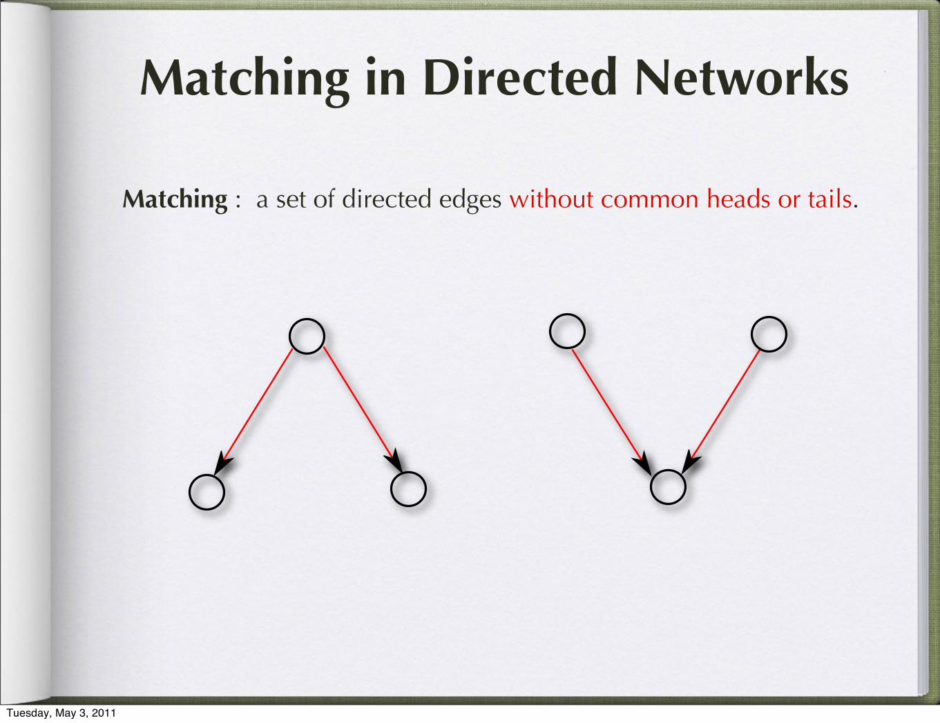
Matching in Directed Networks
Matching : a set of directed edges without common heads or tails.
Tuesday, May 3, 2011

Matching in Directed Networks
Matching : a set of directed edges without common heads or tails.
Not Allowed
Tuesday, May 3, 2011

Matching in Directed NetworksMatching : a set of directed edges without common heads or tails.
Tuesday, May 3, 2011
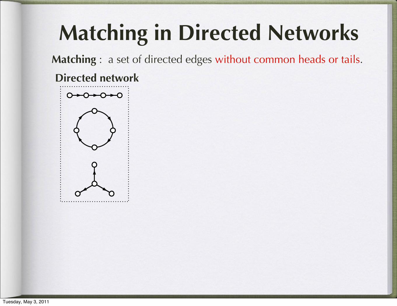
Matching in Directed NetworksMatching : a set of directed edges without common heads or tails.
Directed network
Tuesday, May 3, 2011

Matching in Directed NetworksMatching : a set of directed edges without common heads or tails.
Directed network Maximum matching
Tuesday, May 3, 2011

matched unmatched
Matching in Directed NetworksMatching : a set of directed edges without common heads or tails.
Directed network Maximum matching
Tuesday, May 3, 2011

matched unmatched
Matching in Directed NetworksMatching : a set of directed edges without common heads or tails.
Directed network Maximum matching
Perfect matching
Tuesday, May 3, 2011

matched unmatched
Matching in Directed NetworksMatching : a set of directed edges without common heads or tails.
Directed network Maximum matching
Perfect matching
Minimum Inputs TheoremDriver nodes = unmatched nodes
ND = max{1, Nunmatched}Liu et al., Nature (in press)
Tuesday, May 3, 2011

14
Figure S3: Matching in digraph and its bipartite representation. a, A simple digraph. b, The
bipartite representation of the digraph shown in a. It has a unique maximum matching, which is shown in
red. Matched (or unmatched) nodes are shown in green (or white), respectively.
maximum matching can be found efficiently using the well-known Hopcroft-Karp algorithm, which
runs in O(√
V E) time [23].
Denote |M∗| as the size of the maximum matching in the directed network G(A). We have
Theorem 2 (Minimum Input Theorem).
The minimum number of inputs (NI) or equivalently the minimum number of driver nodes (ND)
need to fully control a network G(A) is one if there is a perfect matching in G(A). (In this case,
any single node can be chosen as the driver node.) Otherwise, it equals the number of unmatched
nodes with respective to any maximum matchings. (In this case, the driver nodes are just the
unmatched nodes.)
NI = ND = max {N − |M∗|, 1} . (S4)
Proof. Case 1) If |M∗| < N , the maximum matching in G(A) is not perfect and there are N− |M∗|
unmatched vertices. The matching edges form elementary paths and circles. We call them matching
paths and matching circles hereafter (see Fig. S2c). We can connect an input vertex to each
unmatched vertex, and form N − |M∗| stems. All other state vertices are spanned by matching
cycles. For a given matching cycle C, if there is an edge e in G(A) such that the starting vertex of
e belongs to one of the stems and the ending vertex of e belongs to C, then e∪C forms a bud. For
a matching cycle which can not form a bud in such a way, we can connect one of the input vertices
to it and form a bud. In both cases, matching cycles do not require extra inputs to form buds.
Thus, we have a disjoint set of cacti with N − |M∗| inputs (origins). According to Lin’s theorem,
the system is structurally controllable. Since |M∗| is the size of the maximum matching in G(A),
How to calculate maximum matchings in Digraph?
A maximum matching of a digraph can be easily found in its bipartite rep-
resentation, using the Hopcroft-Karp algorithm (O(√NE)).
Tuesday, May 3, 2011

Results
Tuesday, May 3, 2011
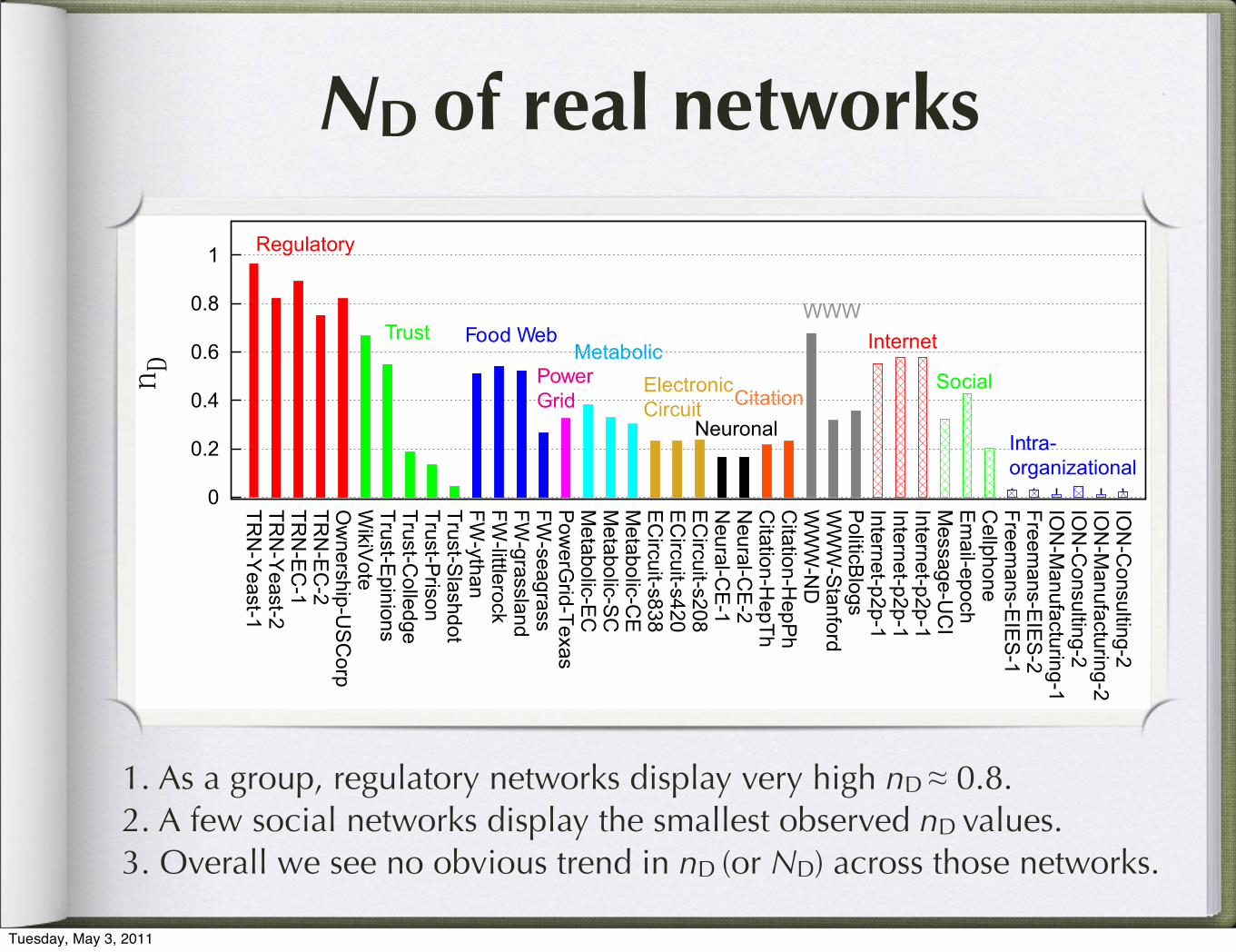
ND of real networksResults: Controllability of Real-world Networks
0
0.2
0.4
0.6
0.8
1
TRN
-Yeast-1
TRN
-Yeast-2
TRN
-EC
-1TR
N-E
C-2
Ow
nership-US
Corp
WikiV
oteTrust-E
pinionsTrust-C
olledgeTrust-P
risonTrust-S
lashdotFW
-ythanFW
-littlerockFW
-grasslandFW
-seagrassP
owerG
rid-TexasM
etabolic-EC
Metabolic-S
CM
etabolic-CE
EC
ircuit-s838E
Circuit-s420
EC
ircuit-s208N
eural-CE
-1N
eural-CE
-2C
itation-HepTh
Citation-H
epPh
WW
W-N
DW
WW
-Stanford
PoliticB
logsInternet-p2p-1Internet-p2p-1Internet-p2p-1M
essage-UC
IE
mail-epoch
Cellphone
Freemans-E
IES
-1Freem
ans-EIE
S-2
ION
-Manufacturing-1
ION
-Consulting-2
ION
-Manufacturing-2
ION
-Consulting-2
nD
Regulatory
Trust Food Web
PowerGrid
MetabolicElectronic Circuit
NeuronalCitation
WWWInternet
Social
Intra-organizational
We find
1 As a group, regulatory networks display very high nD ≈ 0.8.
2 A few social networks display the smallest observed nD values.
3 Overall we see no obvious trend in nD (or ND) across those networks.
Yang Liu, Jean-Jacques Slotine, Albert-Laszlo Barabasi Controllability of Complex Networks
1. As a group, regulatory networks display very high nD ≈ 0.8.2. A few social networks display the smallest observed nD values.3. Overall we see no obvious trend in nD (or ND) across those networks.
Tuesday, May 3, 2011

Role of hubs
!
"#$%& '())*+%& ,(-.%&"#$%& '())*+%& ,(-.%&
! !
!
!/
!/01
!/02
!/03
!/04
!5
!!
! !"# $%&'()* " +,-.'%/"''
"#
"#$
"# "#$
!%"""!
!%"
#
1. The fraction of driver nodes is significantly higher among low degree nodes than among the hubs.
2. Mean degree of driver nodes <kD> is either significantly smaller or comparable to <k>.
Driver nodes tend to avoid hubs.Tuesday, May 3, 2011

NDreal
vs. NDrand
Tuesday, May 3, 2011
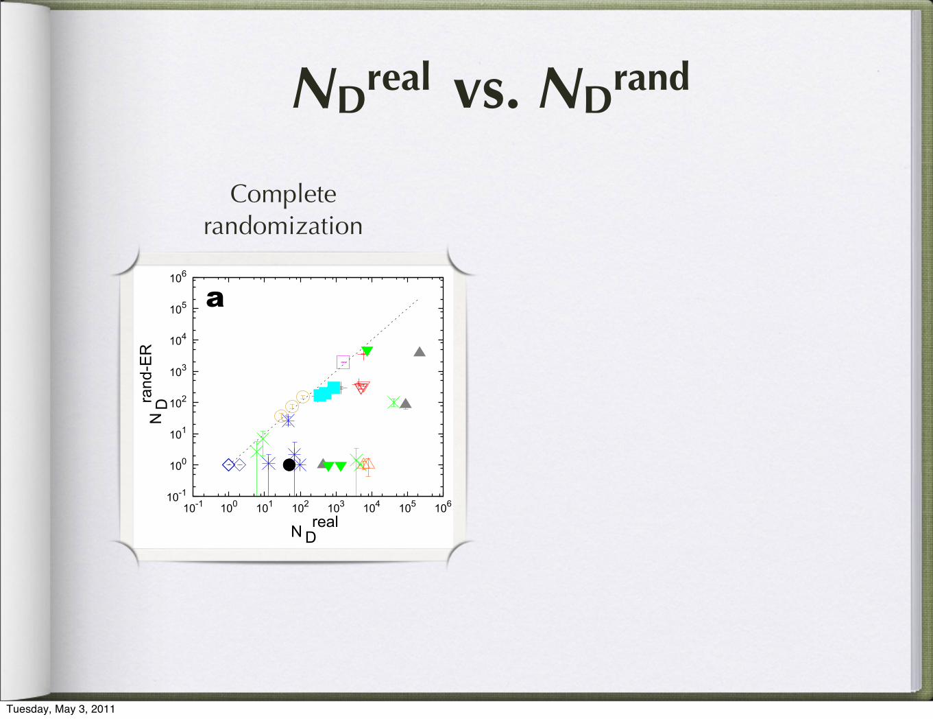
NDreal
vs. NDrand
Results: Compare N realD and N random
D
Two types of randomizations:
a. Complete randomization.Keep N, L unchanged =⇒ Erdos-Renyi random networks.
b. Degree-preserved randomization.Keep N, L, and degree sequence unchanged.
10-1
100
101
102
103
104
105
106
10-1 100 101 102 103 104 105 106
NDrand-ER
N Dreal
a
rand-Degree
Yang Liu, Jean-Jacques Slotine, Albert-Laszlo Barabasi Controllability of Complex Networks
Complete randomization
Degree-preserving randomization
Results: Compare N realD and N random
D
Two types of randomizations:
a. Complete randomization.Keep N, L unchanged =⇒ Erdos-Renyi random networks.
b. Degree-preserved randomization.Keep N, L, and degree sequence unchanged.
10610-1
100
101
102
103
104
105
106
10-1 100 101 102 103 104 105 106NDrand-Degree
N Dreal
b
Yang Liu, Jean-Jacques Slotine, Albert-Laszlo Barabasi Controllability of Complex Networks
ND is mainly determined by degree distribution.
Tuesday, May 3, 2011

Key Result
P (kin, kout) → ND
ND is primarily determined by degree distribution.
Tuesday, May 3, 2011

Key Result
P (kin, kout) → ND
ND is primarily determined by degree distribution.
1. Unexpected and counter-intuitive: The specific wiring diagram does not matter!
Tuesday, May 3, 2011

Key Result
P (kin, kout) → ND
ND is primarily determined by degree distribution.
1. Unexpected and counter-intuitive: The specific wiring diagram does not matter!
2. Allows us to analytically calculate the average ND over all network realizations compatible with P(kin, kout), using the cavity method in statistical physics.
Tuesday, May 3, 2011

Define Q(kout) :=koutP (kout)
�kout� and �Q(kin) :=kin
�P (kin)�kin� .
Generating functions:
G(x) :=�∞
kout=0 P (kout)xkout
�G(x) :=�∞
kin=0�P (kin)xkin
H(x) :=�∞
kout=0 Q(kout + 1)xkout
�H(x) :=�∞
kin=0�Q(kin + 1)xkin
Self-consistent equations:
w1 = H( �w2)w2 = 1−H(1− �w1)
�w1 = �H(w2)
�w2 = 1− �H(1− w1)
Average ND over all network realizations compatible with P (kin, kout)
E(ND) = N2
��G( �w2) +G(1− �w1)− 1
�+
� �G(w2) + �G(1− w1)− 1�
+ z2
��w1(1− w2) + w1(1− �w2)
��
Analytic Result
Tuesday, May 3, 2011

Analytical vs. Numerical
10-1
100
101
102
103
104
105
106
10-1 100 101 102 103 104 105 106
NDrand-Degree
NDanalytic
Tuesday, May 3, 2011

Which properties in P(k)determine ND?
Tuesday, May 3, 2011
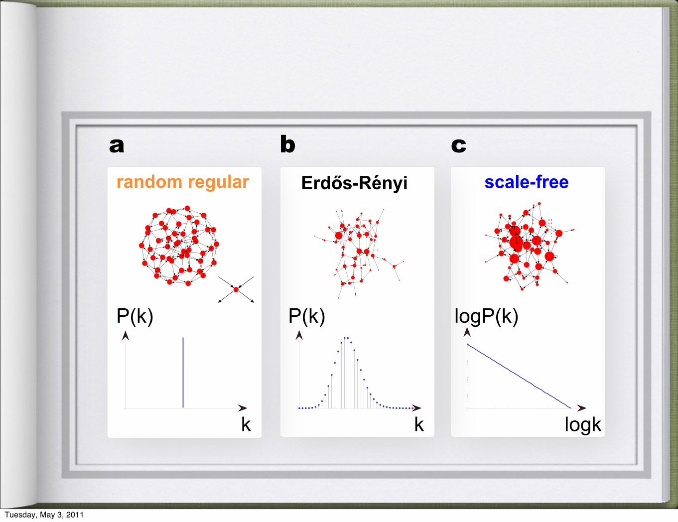
random regular
P(k) P(k) logP(k)
k k logk
Erd s-Renyi scale-free
a b c
d e
f g
10-5
10-4
10-3
10-2
10-1
100
0 10 20 30 40 50
<k>
nD
SF =2.2
SF =3.0
SF =4.0
ER
SF =2.5
N= N=10oo 5
0
0.2
0.4
0.6
0.8
1
1 2 3 4 5 6
SF <k>=2
SF <k>=8
SF <k>=16
SF <k>=4
N= N=10oo 5
nD
All
node
s m
ust b
e co
ntro
lled.
0
0.2
0.4
0.6
0.8
1
0 0.5 1 1.5 2
H
nD
SF <k>=2
SF <k>=8
SF <k>=16
ER
SF <k>=4
N= N=10oo 5
0
0.2
0.4
0.6
0.8
1
0 0.5 1 1.5 2
H
nD
SF =2.2
SF =3.0
SF =4.0
ER
SF =2.5
N= N=10oo 5
22
Most homogeneous Most heterogeneous
Tuesday, May 3, 2011

Results on Model Networks : Infinite System (N = ∞)
Erd s-Renyi Scale-free
0
0.2
0.4
0.6
0.8
1
0 2 4 6 8 10 12 14 16 18 20
<k>
nD
1e-05
0.0001
0.001
0.01
0.1
1
0 4 8 12 16 202e
e- <k> /2
<k>
nD <k>
0
0.2
0.4
0.6
0.8
1
1 2 3 4 5100
101
102
103
104
All
node
s m
ust b
e co
ntro
lled.
Control via a finite fraction of nodes.
nD
ER
nD(�k�) ∼ e−�k�/2 as �k� � 1.
SF, controllability phase transition
nD(γ) → 1 as γ → 2 ⇒ γc = 2 is the critical value!
Yang Liu, Jean-Jacques Slotine, Albert-Laszlo Barabasi Controllability of Complex Networks
Analytical
For infinite system (N = ∞)
1. ER : nD(�k�) ∼ e−�k�/2 as �k� � 1
2. SF : nD(γ) → 1 as γ → γc = 2
Tuesday, May 3, 2011

Finite system, asymptotically (�k� � 1)
1. ER: nD(�k�) ∼ e−�k�/2.
2. SF: nD(�k�, γ) ∼ e−f(γ)�k�/2 with f(γ) = 1− 1γ−1
(consistent with γc = 2).
!"#$
!"#%
!"#&
!"#'
!"#!
!""
(" (!" ('" (&" (%" ($"
!)"
*+
!"# $%&%
!"# $'&(!"# $)&(*+#
!"# $%&,
(((,-((((((((,-!".. $
("
("/'
("/%
("/0
("/1
(!
(! (' (& (% ($ (0
!"#-./$%#
!"#-./$0#!"#-./$12#
!"#-./$)
(((,-((((((((,-!".. $
*+
233(*.456(7869(:5(
;.*9<.3354/
Analytical vs. Numerical
Tuesday, May 3, 2011
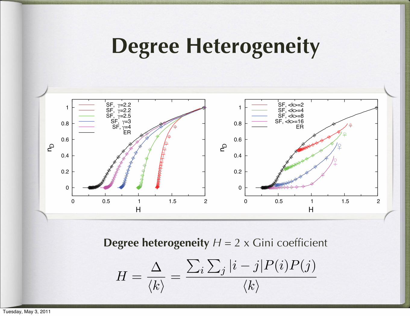
0
0.2
0.4
0.6
0.8
1
0 0.5 1 1.5 2
n D
H
SF, =2.2SF, =2.2SF, =2.5
SF, =3SF, =4
ER
0
0.2
0.4
0.6
0.8
1
0 0.5 1 1.5 2
n D
H
SF, <k>=2SF, <k>=4SF, <k>=8
SF, <k>=16ER
18
w1 ∼ e−z0 , w2 = 1 − e
−z0w1 ∼ z0w1, and thus nD ∼ w1 − z0w1w2 ∼ e−z0 − z
20e−2z0 . Therefore, in
the large z = �k� limit we have
nD ∼ e−z0 = e
−�k�/2. (S51)
To study the effect of degree heterogeneity on nD for an arbitrary network, we defined the
degree heterogeneity as the relative mean difference of its degree distribution,
H =∆�k� =
�i
�j |i− j|P (i)P (j)
�k� = 2�
i
�j<i(i− j)P (i)P (j)
�k� (S52)
where ∆ is the average absolute degree difference of two degrees (i and j) drawn from the degree
distribution. As a measure of statistical dispersion, H has a well-defined range [0, 2] and is twice
of the Gini coefficient of the given distribution. Note that an often used measure of degree hetero-
geneity, �k2�/�k�2, diverges for scale-free networks with γ ≤ 3 in the N → ∞ limit, thus it is not
appropriate to explore the impact of heterogeneity in scale-free networks.
For Poisson distribution: P (k) = e−zzk
k! , k = 0, 1, 2, · · · , one can show that
H = 2e−2z [I0(2z) + I1(2z)] (S53)
where In(x) =�∞
i=01
i!(n+i)!
�x2
�2i+n is the modified Bessel function of the first kind. For a general
distribution P (k), it is usually hard to get an analytical formula for H. Nevertheless, it can be
numerically calculated by using its definition.
3. Exponentially distributed digraph
For exponentially distributed digraphs, we assume both P (kin) and P (kout) follow the same
exponential distribution, i.e. (1− e−1/κ)e−k/κ. Then the half mean degree is given by z0 = z/2 =
e−1/κ
1−e−1/κ = �kin� = �kout� and the generating functions are
G(x) = �G(x) =1− e
−1/κ0
1− xe−1/κ0(S54)
and
H(x) = �H(x) =
�1− e
−1/κ0
1− xe−1/κ0
�2
. (S55)
The calculated nD is shown in Fig. S5.
Degree heterogeneity H = 2 x Gini coefficient
Degree Heterogeneity
Tuesday, May 3, 2011

Summary
1. The minimum set of driver nodes can be efficiently identified,with
ND = max{1, Nunmatched}.
2. ND is mainly determined by the degree distribution.
P (kin, kout) → ND.
* Driver nodes tend to avoid hubs.* Mean degree �k� and degree inhomogeneity H are two main factors.* Sparse and heterogeneous networks are most difficult to control.
Tuesday, May 3, 2011

Courtesy of Mauro MartinoTuesday, May 3, 2011

Many Thanks.We thank Chaoming Song, Ginestra Bianconi, Haijun Zhou, Linas Vepstas, Natali Gulbahce, Hawoong Jeong, Yong-Yeol Ahn, Baruch Barzel, Nicholas Blumm, Dashun Wang, Zehui Qu, and Yanjing Li for valuable discussions.
This work was supported by the Network Science Collaborative Technology Alliance sponsored by the US Army Research Laboratory under Agreement Number W911NF-09-2-0053; the Office of Naval Research under Agreement Number N000141010968; the Defense Threat Reduction Agency Awards WMD BRBAA07-J-2-0035 and BRBAA08-Per4-C-2-0033; and the James S. McDonnell Foundation 21st Century Initiative in Studying Complex Systems.
Tuesday, May 3, 2011

The End
Courtesy of Mauro MartinoTuesday, May 3, 2011


![Robust reconstruction of Baraba´si-Albert networks in the ...dremenik/popularity_networks.pdfsituations ranging from the genome to the Internet [8]. They are generated by a stochastic](https://img.pdfslide.us/doc/110x75/6007292e6406a257c922d834/robust-reconstruction-of-barabasi-albert-networks-in-the-dremenikpopularitynetworkspdf.jpg)


![[1987 J.J. Slotine, W. Li] On the Adaptive Control of Robot Manipulators.pdf](https://img.pdfslide.us/doc/110x75/577c7ab41a28abe05495ece7/1987-jj-slotine-w-li-on-the-adaptive-control-of-robot-manipulatorspdf.jpg)