Control Theory: a Brief Tutorial - Department of Mathematics · PDF fileControl Theory: a Brief Tutorial ... Construct an open-loop control u(t) ... (which start su ciently close to

Control Theory: a Brief Tutorial

Alberto Bressan

Department of Mathematics, Penn State University

[email protected]

Alberto Bressan (Penn State) control theory 1 / 33

ODE’s and control systems x(t) = ddt x(t)

x = f (x) (ODE )

x

x0

x0

f(x)

x

F(x)

x = f (x , u(t)), u(t) ∈ U (control system)

x ∈ F (x) = {f (t, u) ; u ∈ U} (differential inclusion)


Example 1 - boat on a river

x(t) = position of a boat on a river

v(x) velocity of the water

M = maximum speed of the boat relative to the water

x = f (x , u(t)) = v(x) + u(t) u ∈ U = {ω ∈ R2, |ω| ≤ M} (CS)

x ∈ F (x) ={

v(x) + ω ; |ω| ≤ M}

(DI )

x

u

v


Example 2 - cart on a rail

x(t) = position of the cart

y(t) = velocity of the cart

u(t) = force pushing or pulling the cart (control function)

m x = u(t), m = mass of the cart

{x = y

y = 1mu(t)

u(t) ∈ [−1, 1]

0 x

y u


Example 3 - fishery management

x(t) = amount of fish in a lake, at time t

M = maximum population supported by the habitat

u(t) = harvesting effort (control function)

x = αx(M − x)− xu, u(t) ∈ [0, umax ]


Example 4 - systems with scalar control entering linearly

x = f (x) + g(x) u u ∈ [−1, 1]

x ∈ F (x) ={

f (x) + g(x) u ; u ∈ [−1, 1]}

xg

f

x1

0

2


Open-loop controls

If u = u(t) is assigned as a function of time, we say that u is anopen-loop control.

Theorem

Assume that the function f (x , u) is differentiable w.r.t. x. Then for every(possibly discontinuous) control function u(t) the Cauchy problem

x(t) = f (x(t), u(t)), x(t0) = x0

has a unique solution.


Feedback controls

If u = u(x) is assigned as a function of the state variable x , we say thatu is a closed-loop (or feedback) control.

Theorem

Assume that the function f (x , u) is differentiable w.r.t. both x and u, andthat the feedback control function u(x) is differentiable w.r.t. x.Then the Cauchy problem

x(t) = f (x(t), u(x)), x(t0) = x0

has a unique solution.


Designing a control function

x = f (x , u), u(t) ∈ U

Possible goals:

Reach a target in minimum time

Construct a feedback control function u = u(x) which stabilizes thesystem at the origin.

Construct an open-loop control u(t) which is optimal for a given costcriterion.


Two strategies for crossing a river by boat

x

u

v

u

A

B

u

v


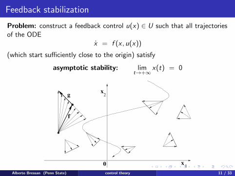
Feedback stabilization

Problem: construct a feedback control u(x) ∈ U such that all trajectoriesof the ODE

x = f (x , u(x))

(which start sufficiently close to the origin) satisfy

asymptotic stability: limt→+∞

x(t) = 0

xg

f

x1

0

2


Asymptotic stabilization by a feedback control

x = f (x , u(x))

x = (x1, . . . , xn) , u = (u1, . . . , um) , f = (f1, . . . , fn)

Theorem

Assume that f (0, u(0)) = 0, so that x = 0 ∈ Rn is an equilibrium point.This equilibrium is asymptotically stable if the n × n Jacobian matrixA = (Aij)

Aij =

[∂fi∂xj

+m∑

k=1

∂fi∂uk

∂uk

∂xj

]x=0

has all eigenvalues with strictly negative real part.


Optimal control problems

x = f (x , u), u(t) ∈ U, x(0) = x0 , t ∈ [0,T ]

x0

F(x)

x

R(T)

R(T) = reachable set

at time T

Goal: Choose a control u(t) ∈ U such that the corresponding trajectorymaximizes the payoff

J = ψ(x(T ))−∫ T

0L(x(t), u(t)) dt

= [terminal payoff]− [running cost]


Existence of optimal controls (with no running cost)

Consider the problem

maximize: ψ(x(T ))

subject to: x = f (x , u), x(0) = x0 , u(t) ∈ U.

Assume that for every x the set of possible velocities

F (x) = {f (x , u) ; u ∈ U}

is closed, bounded, and convex.

Than an optimal (open-loop) control u : [0,T ] 7→ U exists.


Existence of optimal controls (with dynamics linear w.r.t. u)

Consider the problem

maximize: ψ(x(T ))−∫ T

0L(x(t), u(t)) dt

subject to: x = f (x) + g(x)u, x(0) = x0 , u(t) ∈ [a, b].

Assume that the cost function L is convex in u, for every fixed x .

Than an optimal (open-loop) control u : [0,T ] 7→ U exists.


Finding the optimal control

maximize: ψ(x(T ))

subject to: x = f (x , u), x(0) = x0 , u(t) ∈ U

x (t)

ψ = const.

R(T)

*

x0

Let u∗(t) be an optimal control and let x∗(t) be the optimal trajectory.

Derive necessary conditions for their optimality.Alberto Bressan (Penn State) control theory 16 / 33

Preliminary: perturbed solutions of an ODE

x(t) = g(t, x(t)) (ODE )

Let x∗(t) be a solution, and consider a family of perturbed solutions

xε(t) = x∗(t) + εv(t) + O(ε2)

x (t)

v(t)

v( ) x (t)

v(T)

x (T)

x ( )τ*ε

*

x ( )

ε

x (T)ε

*

τ

τ

How does the “first order perturbation” v(t) evolve in time?


An example

x1 = x2 , x2 = − x1 , T = π

1

x2

xx(0) x(T)

x(t)

v(t)

x (t)ε

0


A linearized equation for the evolution of tangent vectors

x(t) = g(t, x(t)) (ODE )

xε(t) = x∗(t) + εv(t) + O(ε2) (†)

Insert (†) in (ODE), and use a Taylor approximation:

xε(t) = g(t, xε(t))

x∗(t) + εv(t) + O(ε2) = g(

t, x∗(t) + εv(t) + O(ε2))

= g(t, x∗(t)

)+∂g

∂x(t, x∗(t)) · εv(t) + O(ε2)

=⇒ v(t) = A(t)v(t), A(t) =∂g

∂x(t, x∗(t))


The adjoint linear system

p = (p1, . . . , pn), v =

v1...

vn

, A(t) is an n × n matrix

Lemma

Let v(t) and p(t) be any solutions to the linear ODEs

v(t) = A(t)v(t), p(t) = − p(t)A(t)

Then the product p(t)v(t) =∑

i pivi is constant.

d

dt(pv) = pv + pv = (−pA)v + p(Av) = 0


Deriving necessary conditions

maximize the terminal payoff: ψ(x(T ))


u∗(t) = optimal control, x∗(t) = optimal trajectory.

x (t)

ψ = const.

R(T)

*

x0

No matter how we change the control u∗(·), the terminal payoff cannot be

increased.


Needle variations

Choose an arbitrary time τ ∈ ]0,T ] and control value ω ∈ U.

needle variation: uε(t) =

{ω if t ∈ [τ − ε, τ ],

u∗(t) otherwise.

perturbed trajectory: xε(t) =

{x∗(t) if t ≤ τ − ε,

x∗(t) + εv(t) +O(ε2) if t ≥ τ

x ∆

ψε

τ−ε

ω

0 Tτ

uε

u* *

*x ( )τ

x (T)

x0

v( )τ

v(T)

ψ = constant


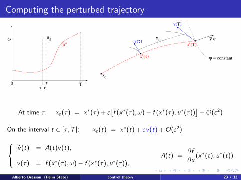
Computing the perturbed trajectory

x ∆

ψε

τ−ε

ω

0 Tτ

uε

u* *

*x ( )τ

x (T)

x0

v( )τ

v(T)

ψ = constant

At time τ : xε(τ) = x∗(τ) + ε[f (x∗(τ), ω)− f (x∗(τ), u∗(τ))

]+O(ε2)

On the interval t ∈ [τ,T ]: xε(t) = x∗(t) + εv(t) +O(ε2),

v(t) = A(t)v(t),

v(τ) = f (x∗(τ), ω)− f (x∗(τ), u∗(τ)),A(t) =

∂f

∂x(x∗(t), u∗(t))


A family of necessary conditions

x ∆

ψε

τ−ε

ω

0 Tτ

uε

u* *

*x ( )τ

x (T)

x0

v( )τ

v(T)

ψ = constant

u∗ is optimal =⇒ d

dεψ(xε(T ))

∣∣∣∣ε=0

= ∇ψ(x∗(T )) · v(T ) ≤ 0


Let the row vector p(t) be the solution to

p(t) = − p(t)A(t), p(T ) = ∇ψ(x∗(T ))

A(t) =∂f

∂x(t, x∗(t))

Since v(t) satisfies v(t) = A(t)v(t), the product p(t)v(t) is constant intime. Hence

p(τ)v(τ) = p(T )v(T ) = ∇ψ(x∗(T )) · v(T ) ≤ 0

For every τ ∈]0,T ] and ω ∈ U, we thus have

p(τ)v(τ) = p(τ)[f (x∗(τ), ω)− f (x∗(τ), u∗(τ))

]≤ 0


Geometric interpretation of the Pontryagin Maximum Principle

For every τ ∈]0,T ], the inequality

p(τ)[f (x∗(τ), ω)− f (x∗(τ), u∗(τ))

]≤ 0 for all ω ∈ U

implies

p(τ) · x∗(τ) = p(τ) · f(x∗(τ), u∗(τ)

)= max

ω∈U

{p(τ) · f

(x∗(τ), ω

)}(PMP)

For every time τ ∈ ]0,T ], the speed x∗(τ) corresponding to the optimal control

u∗(τ) is the one maximizing the product with p(τ).

* τ

*

*.

f(x ( ), )ω

ψ =

p(T) =

const.

∆

x ( )τ

x ( )τx (T)

ψ

x0

p( )τ

*


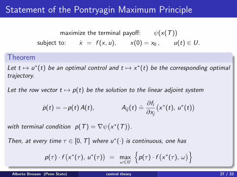
Statement of the Pontryagin Maximum Principle

maximize the terminal payoff: ψ(x(T ))


Theorem

Let t 7→ u∗(t) be an optimal control and t 7→ x∗(t) be the corresponding optimaltrajectory.

Let the row vector t 7→ p(t) be the solution to the linear adjoint system

p(t) = −p(t) A(t), Aij(t).

=∂fi∂xj

(x∗(t), u∗(t)

)with terminal condition p(T ) = ∇ψ

(x∗(T )

).

Then, at every time τ ∈ [0,T ] where u∗(·) is continuous, one has

p(τ) · f(x∗(τ), u∗(τ)

)= max

ω∈U

{p(τ) · f

(x∗(τ), ω

)}Alberto Bressan (Penn State) control theory 27 / 33

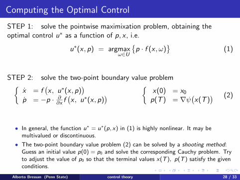
Computing the Optimal Control

STEP 1: solve the pointwise maximixation problem, obtaining theoptimal control u∗ as a function of p, x , i.e.

u∗(x , p) = argmaxω∈U

{p · f (x , ω)

}(1)

STEP 2: solve the two-point boundary value problem{x = f

(x , u∗(x , p)

)p = −p · ∂

∂x f(x , u∗(x , p)

) {x(0) = x0

p(T ) = ∇ψ(x(T )

) (2)

• In general, the function u∗ = u∗(p, x) in (1) is highly nonlinear. It may bemultivalued or discontinuous.

• The two-point boundary value problem (2) can be solved by a shooting method:Guess an initial value p(0) = p0 and solve the corresponding Cauchy problem. Tryto adjust the value of p0 so that the terminal values x(T ), p(T ) satisfy the givenconditions.


Example: a linear pendulum

u

q

q(t) = position of a linearized pendulum, controlled by an external forcewith magnitude u(t) ∈ [−1, 1].

q(t) + q(t) = u(t), q(0) = q(0) = 0, u(t) ∈ [−1, 1]

We wish to maximize the terminal displacement q(T ).


q(t) + q(t) = u(t), q(0) = q(0) = 0, u(t) ∈ [−1, 1]

Equivalent control system: x1 = q, x2 = q

{x1 = f1(x1, x2, u) = x2x2 = f2(x1, x2, u) = u − x1

{x1(0) = 0x2(0) = 0

Goal: maximize ψ(x(T )).

= x1(T )

Let u∗(t) be an optimal control, and let x∗(t) be the optimal trajectory.

The adjoint vector p = (p1, p2) is found by solving the linear system of ODEs

p = − p(t)A(t), p(T ) = ∇ψ(x∗(T ))

Aij(t) =∂fi∂xj

, A(t) =

(0 1−1 0

)ψ(x1, x2) = x1, (p1(T ), p2(T )) =

(∂ψ

∂x1,∂ψ

∂x2

)x=x∗(T )

= (1, 0)


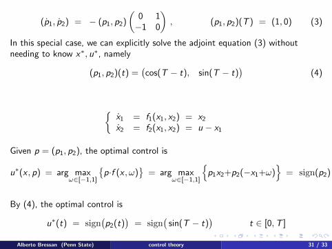
(p1, p2) = − (p1, p2)

(0 1−1 0

), (p1, p2)(T ) = (1, 0) (3)

In this special case, we can explicitly solve the adjoint equation (3) withoutneeding to know x∗, u∗, namely

(p1, p2)(t) =(cos(T − t), sin(T − t)

)(4)

{x1 = f1(x1, x2) = x2x2 = f2(x1, x2) = u − x1

Given p = (p1, p2), the optimal control is

u∗(x , p) = arg maxω∈[−1,1]

{p·f (x , ω)

}= arg max

ω∈[−1,1]

{p1x2+p2(−x1+ω)

}= sign(p2)

By (4), the optimal control is

u∗(t) = sign(p2(t)

)= sign

(sin(T − t)

)t ∈ [0,T ]


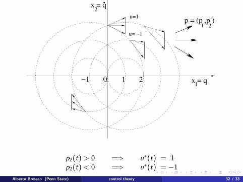
p = (p ,p )1 2

u=1

u= −1

x = q

x = q1

2

0 1 2−1

.

p2(t) > 0 =⇒ u∗(t) = 1p2(t) < 0 =⇒ u∗(t) = −1


References

A. Bressan and B. Piccoli, Introduction to the Mathematical Theory of Control,AIMS Series in Applied Mathematics, Springfield Mo. 2007.

L. Cesari, Optimization - Theory and Applications, Springer, 1983.

W. H. Fleming and R. W. Rishel, Deterministic and Stochastic Optimal Control,Springer, 1975.

S. Lenhart and J. T. Workman, Optimal Control Applied to Biological ModelsChapman and Hall/CRC, 2007.


Documents

Control Theory: a Brief Tutorial - Department of Mathematics · PDF fileControl Theory: a Brief Tutorial ... Construct an open-loop control u(t) ... (which start su ciently close to