Embed Size (px)
Citation preview
Outline
Control systemsFrequency domain analysis
V. Sankaranarayanan
V. Sankaranarayanan Frequency domain analysis
Outline
Outline
1 IntroductionExample
2 Graphical techniquesBode plotExamplesPolar plots
V. Sankaranarayanan Frequency domain analysis

Outline
Outline
1 IntroductionExample
2 Graphical techniquesBode plotExamplesPolar plots
V. Sankaranarayanan Frequency domain analysis

IntroductionGraphical techniques
Example
Frequency response
Definition
Steady state response of a linear system to a sinusoidal input
Advantages
we can use the data obtained from measurements on the physical systemwithout deriving its mathematical model.
It is used to study both the absolute and relative stabilities of linearclosed-loop systems from a knowledge of their open-loop frequency responsecharacteristics.
Frequency-response tests are, in general, simple and can be made accuratelyby use of readily available sinusoidal signal generators and precisemeasurement equipment.
V. Sankaranarayanan Frequency domain analysis

IntroductionGraphical techniques
Example
Historical perspective
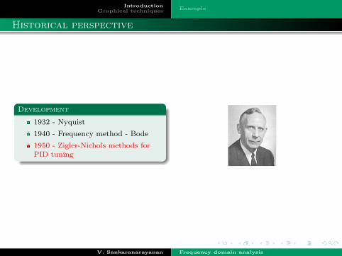
Development
1932 - Nyquist
1940 - Frequency method - Bode
1950 - Zigler-Nichols methods forPID tuning
V. Sankaranarayanan Frequency domain analysis

IntroductionGraphical techniques
Example
Historical perspective
Development
1932 - Nyquist
1940 - Frequency method - Bode
1950 - Zigler-Nichols methods forPID tuning
V. Sankaranarayanan Frequency domain analysis
IntroductionGraphical techniques
Example
Historical perspective
Development
1932 - Nyquist
1940 - Frequency method - Bode
1950 - Zigler-Nichols methods forPID tuning
V. Sankaranarayanan Frequency domain analysis

IntroductionGraphical techniques
Example
Frequency response analysis I
Definition
Steady state response of a linear system to a sinusoidal input
x(t) = X sinωt
G(s) =p(s)
q(s)=
p(s)
(s+ s1)(s+ s2)....(s+ sn)
Y (s) = G(s)X(s) =p(s)
q(s)X(s)
Y (s) = G(s)X(s) = G(s)ωX
s2 + ω2
Y (s) =a
s+ jω+
a
s− jω+
b1
s+ s1+
b2
s+ s2+ .....+
bn
s+ sn
V. Sankaranarayanan Frequency domain analysis

IntroductionGraphical techniques
Example
Frequency response analysis II
y(t) = ae−jωt + aejωt + b1e−s1t + b2e
−s2t + .......+ bne−snt
yss = ae−jωt + aejωt
a = −XG(−jω)
2j
a =XG(jω)
2j
Complex function G(jω) can be written as
G(jω) = |G(jω)|ejφ
φ = ∠G(jω) = tan−1[ imaginarypartofG(jω)
realpartofG(jω)
]yss(t) = X|G(jω)|
ej(ωt+φ) − e−j(ωt+φ)
2j
= X|G(jω)| sin(ωt+ φ)
= Y sin(ωt+ φ)
V. Sankaranarayanan Frequency domain analysis

IntroductionGraphical techniques
Example
Frequency response analysis III
V. Sankaranarayanan Frequency domain analysis

IntroductionGraphical techniques
Example
Outline
1 IntroductionExample
2 Graphical techniquesBode plotExamplesPolar plots
V. Sankaranarayanan Frequency domain analysis

IntroductionGraphical techniques
Example
Example I
Consider the following system
G(s) =K
1 + Ts
G(jω) =K
1 + Tjω
|G(jω)| =K
√1 + T 2ω2
φ = − tan−1 Tω
For the input X sinωt
yss =KX
√1 + T 2ω2
sin(ωt− tan−1 Tω)
V. Sankaranarayanan Frequency domain analysis

IntroductionGraphical techniques
Bode plotExamplesPolar plots
Various methods
Different graphical techniques
Bode diagram or logarithmic plot
Nyquist plot or polar plot
Log-magnitude-versus-phase plot (Nichols plots)
V. Sankaranarayanan Frequency domain analysis

IntroductionGraphical techniques
Bode plotExamplesPolar plots
Outline
1 IntroductionExample
2 Graphical techniquesBode plotExamplesPolar plots
V. Sankaranarayanan Frequency domain analysis

IntroductionGraphical techniques
Bode plotExamplesPolar plots
Bode plot
Bode plot
It consists of two graphs
Logarithm of the magnitude of a sinusoidal transfer function
Phase angle
Both are plotted against the frequency on a logarithmic
logarithmic magnitude of G(jω) is 20 log |G(jω)|Log scale of frequency and the linear scale for magnitude or phase angle
The multiplications of magnitude can be converted into addition
Although it is not possible to plot the curves right down to zero frequencybecause of the logarithmic frequency (log 0 =∞), this does not create aserious problem
V. Sankaranarayanan Frequency domain analysis

IntroductionGraphical techniques
Bode plotExamplesPolar plots
Bode plot
Basic factors
Gain K
Integral and derivative factors (jω)±1
First-order factors (1 + jω)±1
Quadratic factors[1 + 2ζ(j ω
ωn) + (j ω
ωn)2]±1
V. Sankaranarayanan Frequency domain analysis

IntroductionGraphical techniques
Bode plotExamplesPolar plots
Bode plot
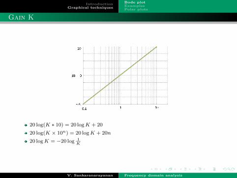
Gain K
A number greater than unity has a positive value in decibels, while a numbersmaller than unity has a negative value.
The log-magnitude curve for a constant gain K is a horizontal straight line atthe magnitude of 20 logKdecibels.
The phase angle of the gain K is zero.
The effect of varying the gain K in the transfer function is that it raises orlowers the log-magnitude curve of the transfer function
V. Sankaranarayanan Frequency domain analysis
IntroductionGraphical techniques
Bode plotExamplesPolar plots
Gain K
20 log(K ∗ 10) = 20 logK + 20
20 log(K × 10n) = 20 logK + 20n
20 logK = −20 log 1K
V. Sankaranarayanan Frequency domain analysis
IntroductionGraphical techniques
Bode plotExamplesPolar plots
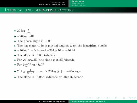
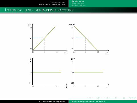
Integral and derivative factors
20 log∣∣∣ 1jω
∣∣∣−20 logωdB
The phase angle is −90o
The log magnitude is plotted against ω on the logarithmic scale
−20 log 1 = 0dB and −20 log 10 = −20dB
The slope is −20dB/decade
For 20 logωdB, the slope is 20dB/decade
For ( 1jω
)n or (jω)n
20 log∣∣∣ 1(jω)n
∣∣∣ = −n× 20 log |jω| = −20n logω
The slope is −20ndB/decade or 20ndB/decade
V. Sankaranarayanan Frequency domain analysis
IntroductionGraphical techniques
Bode plotExamplesPolar plots
Integral and derivative factors
V. Sankaranarayanan Frequency domain analysis
IntroductionGraphical techniques
Bode plotExamplesPolar plots
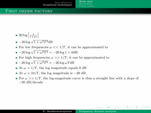
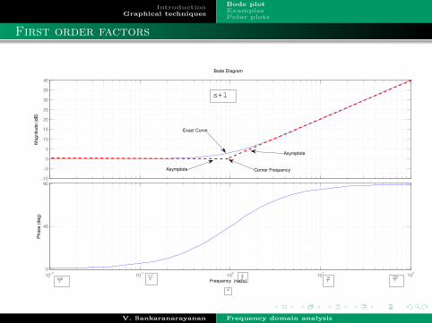
First order factors
20 log∣∣∣ 11+jω
∣∣∣−20 log
√1 + ω2T 2dB
For low frequencies ω << 1/T , it can be approximated to
−20 log√
1 + ω2T 2 = −20 log 1 = 0dB
For high frequencies ω >> 1/T , it can be approximated to
−20 log√
1 + ω2T 2 = −20 logωTdB
At ω = 1/T , the log magnitude equals 0 dB
At ω = 10/T , the log magnitude is −20 dB.
For ω >> 1/T , the log-magnitude curve is thus a straight line with a slope of−20 dB/decade
V. Sankaranarayanan Frequency domain analysis

IntroductionGraphical techniques
Bode plotExamplesPolar plots
First order factors
φ = − tan−1 ωT
At zero frequency φ = 0
At ω = 1/T , φ = −45o
At ω =∞, φ = −90o
V. Sankaranarayanan Frequency domain analysis

IntroductionGraphical techniques
Bode plotExamplesPolar plots
First order factors
−30
−25
−20
−15
−10
−5
0
5
10
Mag
nit
ud
e (
dB
)
10−2
10−1
100
101
102
−90
−45
0
Ph
ase (
deg
)
Bode Diagram
Frequency (rad/s)
Corner Frequency
Asymptote
Asymptote
Exact Curve
V. Sankaranarayanan Frequency domain analysis
IntroductionGraphical techniques
Bode plotExamplesPolar plots
First order factors
−10
−5
0
5
10
15
20
25
30
35
40
Magnitude (
dB
)
10−2
10−1
100
101
102
0
45
90
Phase (
deg)
Bode Diagram
Frequency (rad/s)
Corner Frequency
Asymptote
Asymptote
Exact Curve
s+1
1
T
ω
10
T
100
T
0.1
T0.01
T
V. Sankaranarayanan Frequency domain analysis

IntroductionGraphical techniques
Bode plotExamplesPolar plots
Second order factors
[1 + 2ζ(j ωωn
) + (j ωωn
)2]±1
G(jω) = 11+2ζ(j ω
ωn)+(j ω
ωn)2
20 log∣∣∣ 11+2ζ(j ω
ωn)+(j ω
ωn)2
∣∣∣ = −20 log
√(1− ω2
ω2n
)2 + (2ζ ωωn
)2
For low frequncies ω << ωn
−20 log 1 = 0dB
For high frequencies
−20 log ω2
ω2n
= −40 log ωωn
dB
The slope is −40dB/decade
At ω = ωn
−40 log ωnωn
= −40 log 1 = 0dB
V. Sankaranarayanan Frequency domain analysis

IntroductionGraphical techniques
Bode plotExamplesPolar plots
Second order factors
φ = ∠ 11+2ζ(jω/ωn)+(jω/ωn)2
= − tan−1[ 2ζ ω
ωn1−( ω
ωn)2
]At ω = 0, φ = 0
At ω = ωn, φ = − tan−1 ( 2ζ0
) = − tan−1∞ = −90◦
At ω =∞, φ = −180◦
V. Sankaranarayanan Frequency domain analysis

IntroductionGraphical techniques
Bode plotExamplesPolar plots
First order factors
−40
−30
−20
−10
0
10
20
Magnitude (
dB
)
10−1
100
101
−180
−135
−90
−45
0
Phase (
deg)
Bode Diagram
ω / ωn (rad/s)
ζ =0.1
ζ =0.2
ζ=0.3
ζ=0.5
ζ =0.2
\zeta =0.1
ζ=0.3
ζ=0.5
ζ=0.7
ζ=0.7
ζ=1
\zeta=1
Asymptote
V. Sankaranarayanan Frequency domain analysis
IntroductionGraphical techniques
Bode plotExamplesPolar plots
Outline
1 IntroductionExample
2 Graphical techniquesBode plotExamplesPolar plots
V. Sankaranarayanan Frequency domain analysis

IntroductionGraphical techniques
Bode plotExamplesPolar plots
Examples
G(s) = 5s+10
Time constant formG(s) = 0.51+0.1s
DC Gain - 20 log 0.5
First order factor - Till 10 rad/sec 0db/decade
Slope −20dB/decade from 10 rad/sec
−50
−40
−30
−20
−10
0
Ma
gn
itu
de
(d
B)
10−1
100
101
102
103
−90
−45
0
Ph
ase
(d
eg
)
Bode Diagram
Frequency (rad/s)
Corner Frequency
V. Sankaranarayanan Frequency domain analysis

IntroductionGraphical techniques
Bode plotExamplesPolar plots
More Example
G(s) = s+1s+100
Time Constant Form G(s) =0.01(s+1)0.01s+1
Dc Gain -20log(0.01)=-40dBSlope : Before 1 rad/sec 0dB/decade ,1rad/sec-100 rad/sec 20dB/decade,After 100rad/sec 0db/decade
−40
−35
−30
−25
−20
−15
−10
−5
0
Magnitu
de (
dB
)
10−2
10−1
100
101
102
103
104
0
30
60
90
Phase
(deg)
Bode Diagram
Frequency (rad/s)
Corner Frequency 1
Corner Frequency 100
V. Sankaranarayanan Frequency domain analysis

IntroductionGraphical techniques
Bode plotExamplesPolar plots
Terminology
V. Sankaranarayanan Frequency domain analysis

IntroductionGraphical techniques
Bode plotExamplesPolar plots
Magnitude Plot
Consider
G(s) =5
s= 5×
1
s
20log|G(s)| = 20log(5) + 20log|1
s|
BodeMagnitudeP lot = ConstantLine+−20dBline
100
101
−20
−15
−10
−5
0
5
10
15
Magnitude (
dB
)
Bode Diagram
Frequency (rad/s)
Plot for5
s
Plot for1
s
20log(5)
V. Sankaranarayanan Frequency domain analysis

IntroductionGraphical techniques
Bode plotExamplesPolar plots
Magnitude Plot
G(s) =1000(s+ 1)
s+ 100=
10(s+ 1)
0.01s+ 1
10−2
10−1
100
101
102
103
104
−40
−20
0
20
40
60
80
Magnitude (
dB
)
Bode Diagram
Frequency (rad/s)
Plot for 10.01s+1
20log(10)
Plot for s+ 1
Plot for 10(s+1)0.01s+100
V. Sankaranarayanan Frequency domain analysis

IntroductionGraphical techniques
Bode plotExamplesPolar plots
Phase Plot
Consider =
G(s) =1
s+ 1
G(jω) =1
jω + 1
Angle is ∠G(jw) = − arctan(ω)ω = 0,∠G(jω) = 0o
ω =∞,∠G(jω) = −90o
10−2
10−1
100
101
102
−90
−60
−30
0
Pha
se (
deg)
Bode Diagram
Frequency (rad/s)
Consider =
G(s) = s+ 1
G(jω) = jω + 1
Angle is ∠G(jw) = arctan(ω)ω = 0,∠G(jω) = 0o
ω =∞,∠G(jω) = 90o
10−2
10−1
100
101
102
0
30
60
90
Pha
se (
deg)
Bode Diagram
Frequency (rad/s)
V. Sankaranarayanan Frequency domain analysis

IntroductionGraphical techniques
Bode plotExamplesPolar plots
Sencond Order System
ConsiderG(jω) = (jω)2 + 2ζωnjω + ω2
n
G(jω) = ω2n − ω2 + j2ζωnω
Angle is
∠G(jω) = tan−1
(2ζωnω
ω2n − ω2
)ω = 0,∠G(jω) = 0o
ω =∞,∠G(jω) = 180o
10−2
10−1
100
101
102
0
45
90
135
180
Phase (
deg)
Bode Diagram
Frequency (rad/s)
V. Sankaranarayanan Frequency domain analysis

IntroductionGraphical techniques
Bode plotExamplesPolar plots
Example
G(s) =s+ 1
s+ 100
G(jω) =jω + 1
jω + 10
ω = 0∠G = 0, ω =∞∠G = 0 Supose ω = 30rad/sec,∠G = 16o
10−2
10−1
100
101
102
103
104
−90
−45
0
45
90
Phase (
deg)
Bode Diagram
Frequency (rad/s)
s+1
s+100
s+1
s+100
V. Sankaranarayanan Frequency domain analysis

IntroductionGraphical techniques
Bode plotExamplesPolar plots
More Example
G(s) = s+5(s+1)(s+10)
Time Constant form G(s) = 0.5 0.2s+1(s+1)(0.1s+1)
Dc Gain: -20log(0.5)Asymptote slopes: Upto 1rad/sec = 0dB/decade , 1rad/sec - 5rad/sec =-20dB/decade , 5rad/sec-10rad/sec = 0dB/decade, After 10rad/sec =-20dB/decadeNote: Asymptotic approximation seems to fail because of presence of cornerfrequency near to each other.
−45
−40
−35
−30
−25
−20
−15
−10
−5
Magnitude (
dB
)
10−2
10−1
100
101
102
−90
−60
−30
0
Phase (
deg)
Bode Diagram
Frequency (rad/s)
1rad/sec
5rad/sec
10rad/sec
V. Sankaranarayanan Frequency domain analysis

IntroductionGraphical techniques
Bode plotExamplesPolar plots
More Example
G(s) = s+10(s+1)(s+1000)
Time Constant form G(s) = 1100
0.1s+1(s+1)(0.001s+1)
Dc Gain= -20log(0.01)Slope: Upto 1rad/sec = 0dB/decade , 1rad/sec - 10rad/sec = -20dB/decade ,10rad/sec - 1000rad/sec = 0dB/decade , After 1000rad/sec = -20dB/decadeNote: Asymptotic approximation matches
−100
−90
−80
−70
−60
−50
−40
Magnitude (
dB
)
10−2
10−1
100
101
102
103
104
105
−90
−45
0
Phase (
deg)
Bode Diagram
Frequency (rad/s)
1rad/sec
10rad/sec
1000rad/sec
V. Sankaranarayanan Frequency domain analysis

IntroductionGraphical techniques
Bode plotExamplesPolar plots
More Example
G(s) =s+ 10
(s+ 1)(s2 + 600s+ 1000000)Slops: Upto 1rad/sec = 0dB/decade, 1rad/sec - 10rad/sec = 20dB/decade,10rad/sec - 1000rad/sec= 0dB/decade, After 1000rad/sec= -40dB/decade
−200
−190
−180
−170
−160
−150
−140
−130
−120
−110
−100
Magnitude (
dB
)
10−2
10−1
100
101
102
103
104
105
−180
−90
0
90
Phase (
deg)
Bode Diagram
Frequency (rad/s)
1rad/sec
10rad/sec 1000rad/sec
V. Sankaranarayanan Frequency domain analysis

IntroductionGraphical techniques
Bode plotExamplesPolar plots
Phase margin and gain margin
Gain cross over frequency
It is the frequency at which |G(jω)|, the magnitude of the open-loop transferfunction, is unity
Phase margin
The phase margin is the amount of additional phase lag at the gain cross overfrequency required to the verge of instability γ = 180o + φ
Gain margin
The gain margin is the reciprocal of the magnitude |G(jω)| at the frequency atwhich the phase angle is −180o(Phased cross over frequency)
Kg =1
|G(jω)|= −20 log |G(jω)|
V. Sankaranarayanan Frequency domain analysis

IntroductionGraphical techniques
Bode plotExamplesPolar plots
Terminology
V. Sankaranarayanan Frequency domain analysis

IntroductionGraphical techniques
Bode plotExamplesPolar plots
Terminology
V. Sankaranarayanan Frequency domain analysis

IntroductionGraphical techniques
Bode plotExamplesPolar plots
Outline
1 IntroductionExample
2 Graphical techniquesBode plotExamplesPolar plots
V. Sankaranarayanan Frequency domain analysis

IntroductionGraphical techniques
Bode plotExamplesPolar plots
Polar plot
It is a plot of the magnitude of G(jω) versus the phase angle of G(jω) onpolar coordinates as ω is varied from zero to infinity
In polar plots a positive (negative) phase angle is measured counterclockwise(clockwise) from the positive real axis
V. Sankaranarayanan Frequency domain analysis

IntroductionGraphical techniques
Bode plotExamplesPolar plots
Integral and derivative factors
Integral and derivative factors
G(jω) = 1jω
= −j 1ω
= 1ω∠−90o
The Polar plot of 1jω
is the negative imaginary axis
V. Sankaranarayanan Frequency domain analysis

IntroductionGraphical techniques
Bode plotExamplesPolar plots
Integral and derivative factors
Integral and derivative factors
The Polar plot of jω is the positive imaginary axis
V. Sankaranarayanan Frequency domain analysis

IntroductionGraphical techniques
Bode plotExamplesPolar plots
First order factors
First order factors
G(jω) = 11+jωT
= 1√1+ω2T2
∠−tan−1ωT
G(j0) = 1∠0o, G(j 1T
) = 1√2∠45o
ω −→∞, |G(jω)| −→ 0 and ∠G(jω) −→ −90o
V. Sankaranarayanan Frequency domain analysis

IntroductionGraphical techniques
Bode plotExamplesPolar plots
First order factors
First order factors
G(jω) = 1 + jωT
It is simply the upper half of the straight line passing through point (1, 0) inthe complex plane and parallel to the imaginary axis
V. Sankaranarayanan Frequency domain analysis

IntroductionGraphical techniques
Bode plotExamplesPolar plots
Quadratic factors
Quadratic factors
G(jω) = 11+2ζ(j ω
ωn)+(j ω
ωn)2
For ζ > 0
limω→0
G(jω) = 1∠0
limω→∞
G(jω) = 0∠−180
The polar plot of this sinusoidal transfer function starts at 1∠0 and ends at0∠−180 as ω increases from zero to infinity
The high-frequency portion of G(jω) is tangent to the negative real axis.
For the underdamped case ω = ωn, the phase angle is −90
In the polar plot, the frequency point whose distance from the origin ismaximum corresponds to the resonant frequency ωr.
V. Sankaranarayanan Frequency domain analysis

IntroductionGraphical techniques
Bode plotExamplesPolar plots
V. Sankaranarayanan Frequency domain analysis

IntroductionGraphical techniques
Bode plotExamplesPolar plots
Quadratic factors
Quadratic factors
G(jω) = 1 + 2ζ(j ωωn
) + (j ωωn
)2
=(
1− ω2
ω2n
)+ j(
2ζωωn
)limω→0
G(jω) = 1∠0
limω→∞
G(jω) =∞∠180
V. Sankaranarayanan Frequency domain analysis

IntroductionGraphical techniques
Bode plotExamplesPolar plots
V. Sankaranarayanan Frequency domain analysis