Embed Size (px)
Citation preview
CONTROL SYSTEM FOR A HIGH PULSE-ENERGY
ATMOSPHERIC LIDAR
A Thesis
Presented
to the Faculty of
California State University, Chico
In Partial Fulfillment
of the Requirements for the Degree
Master of Science
in
Electrical and Computer Engineering
by
c© Denton R Scott 2012
Fall 2012


PUBLICATION RIGHTS
No portion of this thesis may be reprinted or reproduced in any manner
unacceptable to the usual copyright restrictions without the written permission of
the author.
iii

ACKNOWLEDGMENTS
The research described herein was supported by awards 0924407,
1104342, and 1228464 from the U.S. National Science Foundation’s Physical and
Dynamic Meteorology Program. The author thanks Dr. Laurie Albright and
committee members for helpful suggestions in preparation of the thesis. Mr. Bruce
Morley and Dr. Scott Spuler of the National Center for Atmospheric Research
(NCAR) provided much appreciated technical assistance. The author thanks the
many family members and friends that provided help and support.
iv

TABLE OF CONTENTS
PAGE
Publication Rights ........................................................................... iii
Acknowledgments ............................................................................ iv
Table of Contents ............................................................................ v
List of Tables.................................................................................. vii
List of Figures ................................................................................ viii
List of Abbreviations ........................................................................ xi
Abstract ........................................................................................ xii
CHAPTER
I. Introduction .................................................................... 1
Narration of Problem ................................................. 1Scope of the Thesis.................................................... 2Significance of the Thesis ............................................ 3Preview of Chapters 2 Through 5 ................................. 5
II. Literature Review ............................................................. 7
Lidar History, Technology, and Uses .............................. 7Control Theory ......................................................... 11
III. History and Components of the Raman-Shifted Eye-SafeAerosol Lidar .............................................................. 15
History of the Raman-Shifted Eye-Safe Aerosol Lidar ....... 15Description of the Raman-Shifted Eye-Safe Aerosol
Lidar as Currently Configured ................................ 17
IV. Experimental Procedures, Findings, and Solutions ................... 22
System Variables....................................................... 23
v

CHAPTER PAGE
Laser Energy Control ................................................. 38Safe-Shutdown Feature ............................................... 54Contact Personnel Feature .......................................... 57Frequency of Control ................................................. 58Data Quality ............................................................ 64Testing and Results ................................................... 76
V. Summary ........................................................................ 79
References ...................................................................................... 81
Appendices
A. Future Work .................................................................... 93B. An Overview of the LabVIEW Code for the REAL.................. 102
vi

LIST OF TABLES
TABLE PAGE
1. System Components and Corresponding LocationNumbers for Fig. 5 and 6 .............................................. 25
2. System Variable Measurements Distinguished byDependency on Nd:YAG Laser Pulse ............................... 60
3. Loop Process Time for Distinct Implementation Phases ............ 62
4. Full-Scale Programmable Input Range and VerticalOffset for the NI PCI-5122............................................. 65
5. BSCAN Data File 30-Word Header Format ............................ 74
vii

LIST OF FIGURES
FIGURE PAGE
1. General Control System Diagram ......................................... 11
2. Gain Scheduler Feedback Control System Diagram .................. 12
3. Linear Feedback Control System Diagram.............................. 13
4. Photograph of the Lidar at the CSUC Farm........................... 21
5. Cutaway of a Solid-Model of the Lidar System........................ 26
6. Diagram of Component Placement on Optics Table ................. 27
7. Control System Hardware Component Signal Flow Diagram ...... 28
8. Photograph of the Two Gravity Referenced Tiltmeters ............. 33
9. Photograph of the Precipitation Sensor ................................. 35
10. Photograph of the DataRay WinCamD Beam Profiler inthe Transmitter of the Instrument ................................... 36
11. Typical Beam Profile Produced by the DataRayWinCamD CCD Camera ............................................... 37
12. Time-Series of Several Vital Signs during the 2007 CHATSExperiment ................................................................ 39
13. Lidar Control System Diagram with Energy Feedback Loop ...... 41
14. Time vs. Laser Energy and Conversion Efficiency duringthe 11 Increments of the Flashlamp Voltage ...................... 42
viii

15. Photograph of the Flashlamps Discharging in the Nd:YAGLaser Cavity ............................................................... 43
16. Photograph of the Damaged Raman Cell Prism ...................... 44
17. Color Negative Burn Paper Results from FlashlampVoltage vs. Conversion Experiment ................................. 46
18. Energy Density of the Nd:YAG beam at 1 µm vs.Distance from the Raman Cell Entry Window perFlashlamp Voltage ....................................................... 47
19. Lidar Control System Diagram with Pulse CountFeedback Controller ..................................................... 49
20. Vital Signs during the October 2012 Experiment usingthe Gain Scheduling Controller with Pulse Count Feedback .. 51
21. A Comparison of Data from the CHATS Experiment andthe Field Experiment with Flashlamp Voltage Control ........ 53
22. Photograph of Nd:YAG Laser PCU Power Key Turner ............. 55
23. Photograph of the Receiver Box Safety Shutter ....................... 56
24. Backscatter Intensity Waveforms from InGaAs Detectorson Days with Clear Sky, Clouds, and a Smoke Layer ........... 66
25. Frequency Distribution of Single Pulse SNR of the AerosolBackscatter Data as a Function of Range during theCHATS Experiment ..................................................... 67
26. Frequency Distribution of Single Pulse SNR of the AerosolBackscatter Data as a Function of Range during theFlashlamp Voltage Control Field Experiment .................... 68
27. Comparison of SNR Peak Distribution of the AerosolBackscatter Data as a Function of Range duringthe Control System Field Experiment .............................. 70
28. Distributions of Wind Velocity Component Differencesas a Function of Average SNR ........................................ 71
ix

29. Comparison of Unnormalized and Normalized Full Scan Data .... 72
30. Magnified Comparison of Unnormalized and NormalizedFull Scan Data ............................................................ 72
31. BSCAN File Format Organization........................................ 73
x

LIST OF ABBREVIATIONS
BSCAN - format designator given to the raw REAL beam-by-beam data
BSU - Beam Steering Unit
CHATS - Canopy Horizontal Array Turbulence Study
CSUC - California State University, Chico
InGaAs - Indium Gallium Arsenide
Lidar - Light Detection and Ranging
LUT - Look-Up Table
Nd:YAG - Neodymium-doped Yttrium Aluminum Garnet
NI - National Instruments
PCU - Power and Cooling Unit
PID - Proportional, Integral, Derivative (control method)
REAL - Raman-shifted Eye-safe Atmospheric Lidar
RTOS - Real-Time Operating System
SNR - Signal to Noise Ratio
SRS - Stimulated Raman Scattering
UPS - Uninterruptible Power Supply
xi

ABSTRACT
CONTROL SYSTEM FOR A HIGH PULSE-ENERGY
ATMOSPHERIC LIDAR
by
c© Denton R Scott 2012
Master of Science in Electrical and Computer Engineering
California State University, Chico
Fall 2012
A master’s thesis that develops, tests, and implements a control system
for a high pulse-energy atmospheric lidar system is presented. The control system
senses in real-time system variables such as transmitter component temperature,
pressure, and energy and diameter of high energy laser pulses and makes decisions
on whether action is required. The control program can immediately and gracefully
shut down the lidar if the system variable measurements exceed operator-defined
thresholds. It can also inform operators of changes in system status. The control
system includes a feedback loop to increase the Neodymium-doped Yttrium
Aluminum Garnet laser flashlamp voltage incrementally thereby providing
improved transmit pulse-energy stability over the 23 to 30 day lifetime of a
flashlamp set. This control system facilitates unattended operation of the lidar over
long periods of time with more uniform performance and the safety of a control
system that can head off potentially catastrophic system failures.
xii

CHAPTER I
INTRODUCTION
Narration of Problem
Improved spatial wind field and atmospheric boundary layer height
measurements are needed in a number of practical applications. Wind resource
assessment requires long-term monitoring to determine wind energy potential in
challenging to reach locations and altitudes (for example, offshore
measurements) [1]-[4]. Wind turbines are more efficient if incoming wind vector
measurements are used to optimize the pitch of rotor blades and yaw of the hub [5].
Air quality forecasting can be improved with measurements of boundary layer
height [6], [7]. Dispersion of potentially hazardous emissions from industrial sites
can be tracked [8]. Airport safety and efficiency can be increased with observations
of wake vortices and wind shears that may be hazardous to aircraft [9]-[11].
Scanning lidars enable remote observations of the two dimensional
spatial structure and movement of the clear atmosphere. As a lidar scans, pulses of
radiation propagate through the atmosphere illuminating volumes containing air
molecules, aerosol particles, and hydrometers. A small portion of the radiation is
scattered back to the lidar where the intensity is detected and recorded. Horizontal
scans reveal the advection of features, such as aerosol plumes, as they drift with the
wind. Vertical scans reveal the atmospheric boundary layer that tends to contain a
higher density of aerosol particles in contrast to the rest of the troposphere which is
1

2
more clear. Computer algorithms can be applied to the image sequences to
determine the wind field and atmospheric boundary layer height [12], [13].
The Department of Physics at California State University, Chico
(CSUC) operates a scanning lidar for atmospheric research. This instrument is
well-suited to measure the wind field and atmospheric boundary layer height as (1)
the laser pulses emitted into the atmosphere have high peak power and yet are
eye-safe, (2) cross-sections of the atmosphere are produced quickly (one scan
approximately every 15 seconds), and (3) computer algorithms implemented by the
research group can calculate two-component wind vectors from sequential scans
and atmospheric boundary layer heights from individual scans [12].
The above applications require spatial wind field and boundary layer
height measurements to be collected over long periods of time. In order to be
cost-efficient and reliable over long periods of time (months, preferably years), the
high pulse-energy atmospheric lidar at CSUC must operate continuously,
unattended, and in a fail-safe manner. This study addresses these challenges.
Scope of the Thesis
This study develops a control system for a high pulse-energy atmospheric
lidar to facilitate continuous, unattended, and fail-safe operation. System failure
cases were analyzed and characteristics of the system operation were explored.
Specific system components and processes were optimized to improve data quality
and control. A field experiment was conducted with the proposed control system in
place. Data were collected and performance was compared to that of a previous
experiment that used a design with no control system [14]-[16]. Recommendations
are provided for future work that will lead to enhanced performance.

3
Significance of the Thesis
This study represents a milestone in the development of the instrument
at CSUC: the first automatic flashlamp voltage adjustment and fail-safe operation
of the high pulse-energy atmospheric lidar. This instrument transmits high energy,
eye-safe pulses into the atmosphere at a rate of 10 Hz. Each pulse produces
backscatter radiation with a sufficiently high signal-to-noise ratio (SNR) that, after
a 15 second scan of the atmosphere, spatial atmospheric structure is revealed to
ranges typically up to 3 to 5 km. This high performance is largely the result of the
high energy transmitter which, in particular, benefits from a control system.
The SNR of backscatter radiation data is affected by the conditions of
the atmosphere as well as the performance of the instrument. For example, an
increase in atmospheric particle concentration will result in stronger SNR.
Similarly, reduction of electronics noise in the receiver subsystem will result in
stronger SNR. Given a constant atmosphere, the SNR is strongly dependent upon
the “power-aperture product” of the lidar [17]. An increase in SNR may be the
result of an increase in power transmitted or an increase in receiver aperture size.
There are different ways to obtain the same power-aperture product.
Consider two lidars with equivalent receiver apertures. One lidar
transmits high energy pulses and the other low energy pulses. Both lidars can have
the same power-aperture product if equal amounts of power are transmitted into
the atmosphere. Transmit power is equal to the total transmit energy per unit of
time. The lidar used in this study nominally transmits 170 mJ of energy into the
atmosphere every 0.1 seconds. A lidar with a pulse-energy of 1 mJ could achieve an
equivalent power-aperture product by integrating over the energy of 170 pulses
emitted in the same 0.1 seconds time interval.

4
The lidar at CSUC transmits high energy pulses to facilitate rapid
scanning of the atmosphere. High energy pulses produce sufficient SNR typically
out to 5 km in range with one pulse and, therefore, eliminate the need to integrate
over backscatter radiation from multiple pulses. In order to produce the high
energy pulses, a flashlamp pumped Nd:YAG laser is used. As the cathodes
deteriorates slightly with each pulse of the 20 million pulse lifetime (about 23 days)
of each flashlamp set, the flashlamp energy emission decreases [18]. This decrease
in flashlamp energy reduces the energy that produces 1 µm pulses in transmitter.
This degradation, if left unchecked, ultimately results in slowly decreasing transmit
energy of the lidar. Flashlamp voltage adjustment is, therefore, required to
maintain the desired transmit energy level. In order for this high energy transmit
pulse to be eye-safe, a Raman cell is used to convert the high energy 1 µm Nd:YAG
pulse to a more eye-safe wavelength of 1.5 µm. Otherwise, the non-eye-safe nature
of the high energy transmit pulse would limit the practical applications of the lidar.
Micropulse is a class of lidar that, in contrast to the lidar at CSUC,
transmit low energy pulses that do not pose as great a risk to optics and system
components. These pulses are typically produced by diode-pumped solid-state
lasers that have a lifetime of more than a year (more than a billion pulses) and
require no significant voltage adjustment to maintain a desired transmit energy
level [19]. However, atmospheric micropulse lidars do not usually scan the
atmosphere. To produce the equivalent SNR of a high pulse-energy lidar, a
micropulse lidar must integrate over the backscatter radiation of multiple pulses
(usually thousands). This integration necessitates slowing the scan in order to
reveal small spatial scale aerosol features in the area of interest. Slowing a scan
defeats the purpose which is to capture images before wind and turbulence have
advected and distorted the aerosol features appreciably. Micropulse lidars typically

5
stare in a single direction and observe atmospheric particulate matter in the path
(often a vertical column) of the pulses over time [20]-[22]. This method of
observation is limited in comparison to the spatial atmospheric cross-sections
observed over time with a scanning lidar.
Because the instrument used in this study incorporates a high pressure
cell containing flammable gas and a laser that produces a beam capable of high
energy densities, failures have the potential to escalate quickly. An increase in the
energy density of the laser beam may damage optics and sensors in the system.
Diffraction patterns caused by one damaged optic may lead to damage (such as
coating failures and inclusions) on others as well. Although it has never happened,
it is conceivable that such failures may initiate a chain of events culminating in a
catastrophic failure such as a rupture in the window of the high pressure cell.
A control system is needed to detect and prevent problems from
escalating during long-term, unattended operation of the instrument. The high
pulse-energy atmospheric lidar at CSUC, with the control system presented in this
study, will facilitate advancements in meteorological research by encouraging
routine long-term, unattended use of the instrument in studies of the wind and
atmospheric boundary layer height.
Preview of Chapters 2 Through 5
Chapter II is a brief review of the theories that apply to the lidar system
used and control systems tested in this study. Chapter III is a history and technical
description of the specific lidar system used in this study. Chapter IV describes the
experimental work conducted, including sensors and subsystems used by the
control system that was developed and tested. Chapter V is a summary of the
thesis. Appendix A lists future engineering projects that would further improve the

6
lidar. Appendix B provides an overview of the control system as written in the
LabVIEW programming language.

CHAPTER II
LITERATURE REVIEW
Lidar History, Technology, and Uses
Although the term lidar was not conceived until the 1950s, light
detection and ranging technology have roots as far back as the 1930s. Even though
lidar technology originated from searchlights and telescopes, in 1938 flashlamps
were used to send pulses of light into the atmosphere that would reflect off cloud
formations. Light pulse round-trip time measurements were used to calculate the
altitude of clouds. This was the first application of atmospheric lidar [23].
The invention and development of the laser in the 1960s opened new
possibilities for lidar technology [24]. Soon lidars were transmitting high energy
pulses at specific wavelengths. This was the launch point from which both laser
and lidar technologies rose to their present importance. Today lidar most
commonly refers to the use of laser radiation detection. In 1976, E. D. Hinkley
further validated lidar technology with the publication of the first lidar text book,
Laser Monitoring of the Atmosphere [23], [25].
Today, lidar technology is commonly used for remote velocity detection
of hard targets (lidar gun) [26]; terrain mapping [27]; scene scanning [28], [29]; and,
as in this study, remote sensing of atmospheric and meteorological variables such as
wind, aerosol, and boundary layer heights [30]-[36]. The instrument used for this
study is an active, high pulse-energy, distributed target (atmospheric) lidar. It is
distinct from hard-target lidars that have the benefit of a bright impulse returned
7

8
from solid objects. The atmospheric lidar must detect backscatter signal from
microscopic particles distributed through the atmosphere.
Active vs. Passive Sensing
Active sensing technologies, such as lidar and radar, involve emitting
energy and sensing the backscatter energy as it encounters targets of interest. In a
lidar, a telescope collects this backscatter energy and, with the help of additional
smaller optics, focuses it onto a photo detector. A passive sensing instrument (i.e.,
a radiometer) senses radiation from sources.
Cameras use both passive and active sensing. When capturing outside
photographs on a sunny day, a common camera will sense that light is sufficient
and not require a flash. This is passive sensing. A dark environment requires active
sensing. Using the flash bulb, the camera emits broadband radiation and captures
the radiation reflected from distant surfaces. The lidar in this study is an active
sensing instrument and the subject is the clear atmosphere. However, unlike a
camera, the lidar provides range-resolved information.
Hard vs. Distributed Target
Laser radiation from a lidar can be used to detect hard or distributed
targets. Because hard target backscatter radiation is relatively intense, lidars for
this application do not in general require high pulse-energy transmitters. Hard
targets produce a large signal-to-noise ratio (SNR) impulse that allows precise
measurements of round-trip time (for target distance measurements) or frequency
shift (for target velocity measurements).
Lidars that sense distributed targets measure range-dependent,
backscatter intensity from air particulate matter (aerosol particles), and
hydrometers (clouds and precipitation) [37]-[39]. For example, when radiation is
emitted into the atmosphere, the population of particles in the path of the pulse
9
scatter very low quantities of energy back to be detected by the instrument [37]. As
the pulse propagates through the atmosphere, radiation is scattered and detected
by the lidar as a function of time. The initial backscatter radiation detected
represents aerosol backscatter intensity at short ranges and delayed radiation
represents aerosol backscatter intensity at longer ranges. This backscatter energy
can be detected until the pulse encounters a hard target or the pulse-energy is
attenuated below an SNR equal to one. The targets detected in this study are
distributed aerosol particles and any backscatter intensity data point represents the
collective backscattering radiation resulting from a very large number of particles.
This is a result of the size of the lidar pulse which illuminates a large volume of
particles at any one instant.
A lidar that senses distributed targets may detect one or both of two
forms of scattering: elastic or inelastic. Elastic scattering describes a process
whereby radiation incident on a particle is redirected and no wavelength change
occurs because the incident radiation is not absorbed by the particle. Inelastic
scattering (includes, for example, Raman and florescence scattering) describes a
process whereby incident radiation is absorbed by a particle and re-emitted as
radiation at a different wavelength. Both elastic and inelastic scattering are
involved in the lidar used in this study. The lidar detects elastic backscatter from
atmospheric particles (radiation transmitted and radiation detected have the same
wavelength of 1.5 µm). However, inelastic scattering takes place in the Raman cell
of the transmitter (radiation enters the cell at a wavelength of 1 µm and a
percentage is absorbed and re-emitted at a wavelength of 1.5 µm). The inelastic
scattering in the Raman cell is known as stimulated Raman scattering (SRS).
Therefore, the elastic lidar used in this study is not to be confused with “Raman

10
lidars” which detect inelastic backscatter radiation at a wavelength different from
that transmitted [40]-[42].
Low vs. High Energy
Lidars may be categorized based on the manner in which they deliver
power: high pulse rate, low energy pulses (micropulse) [43] and low pulse rate, high
energy pulses [44]. In designing a lidar, engineers have the choice of transmitting
one high energy pulse that could have the equivalent SNR of a large number of
weaker pulses. Because of the reliability of a low pulse-energy transmitter, there are
more low pulse-energy lidars in operation. A low pulse-energy laser requires a faster
pulse rate to produce equivalent power and photon-counting (digital) receivers are
generally used to detect the weak backscatter signal [31]. Low pulse-energy laser
also present a lower risk to system components such as optics and sensors.
Alternately, a high pulse-energy laser presents a greater risk of damaging
components during routine operation and, therefore, requires careful monitoring.
However, the high pulse-energy laser does not need to pulse as frequently to
produce the same average power as a low pulse-energy laser.
Though the most popular applications of low pulse-energy lidars sense
hard target returns such as lidar guns, terrain mapping, and scene scanning, there
are also distributed target applications for low pulse-energy lidars in atmospheric
research [45]. High pulse-energy lidars are more commonly applied in the remote
sensing of atmospheric quantities. This study uses a high pulse-energy lidar.
Rayleigh vs. Mie Scattering
Distributed targets scatter radiation in all directions as the pulses
propagate through the atmosphere. Two theories describe how distributed targets
of different size scatter electromagnetic radiation [46]. Two types of elastic
scattering are Rayleigh and Mie. Rayleigh scattering theory describes the

11
redirection of electromagnetic radiation that occurs when the particles are much
smaller than the wavelength of the radiation [47], [48]. For example, visible
radiation with a wavelength of about 0.5 microns will cause Rayleigh scattering as
it propagates through pure air since nitrogen and oxygen molecules are more than
1000 times smaller. The lidar used in the study transmits laser radiation at 1.54
microns wavelength. Therefore, Rayleigh scattering is also produced from the
air [49]. However, the intensity of Rayleigh scattering scales as the one over
wavelength to the 4th power. Therefore, Rayleigh scattering from the lidar is
extremely weak. Most of the backscatter radiation detected by the REAL can be
described through Mie Scattering theory which applies when the particles are
spherical and approximately the same size as the wavelength of the radiation.
Control Theory
Control theory, an aspect of dynamic system engineering, guides a given
system to a desired output by using a previous output to alter an input to that
system. The control uses one or more system outputs in an algorithm that
calculates the next input for the system. One or more system measurement outputs
are input to the control as a feedback variable. Fig. 1 illustrates a general control
system flow diagram.
Fig. 1. General control system diagram.

12
Gain scheduling is one method of control. Gain scheduling maps a
control input directly to a control output using a look-up table [50]. This is a
common controller for simple, robust dynamic systems [51]. The control separates
system operating conditions into areas to be analyzed individually. For the current
area of operation, the pre-calculated control gains are applied to the control
algorithm to produce the desired system response. Fig. 2 illustrates the system
flow diagram.
Gain scheduler controllers have a wide range of applications, from linear
controllers applied to known linear dynamic systems, to adaptive controllers
applied to time-variant, nonlinear dynamic systems. The proportional, integral,
and derivative (PID) controller is commonly used in conjunction with the gain
scheduler method. Because each of the three gains correlates with a response
characteristic, the PID controller is a comprehensive method of control. The
proportional gain adjusts the rise-time, the integral gain adjusts the state-steady
error, and the derivative gain adjusts the settling-time of the response.
Given the system characteristics in the form of a system transfer
function and known operating conditions, the three PID controller gains can be
calculated using a number of known methods. However, this control may perform
Fig. 2. Gain scheduler feedback control systemdiagram.
13
better under one range of operating conditions than another. The gain scheduling
method calculates the three PID gains for several ranges of operation. These gains
are then loaded into a look-up table in the controller design. As the system
operating conditions change, the controller applies the gains optimally calculated
for that range of conditions.
An airplane operating at a wide range of altitudes illustrates this
method. The altitude control may be calculated to perform over the whole range.
This may result in a desirable response at mid-range altitudes, but low and high
altitude responses may suffer. A gain scheduler control could have three sets of
control gains, one each for low, mid-range, and high altitude operating conditions.
This same approach can also be used for the velocity control and other
characteristics that change with operating conditions.
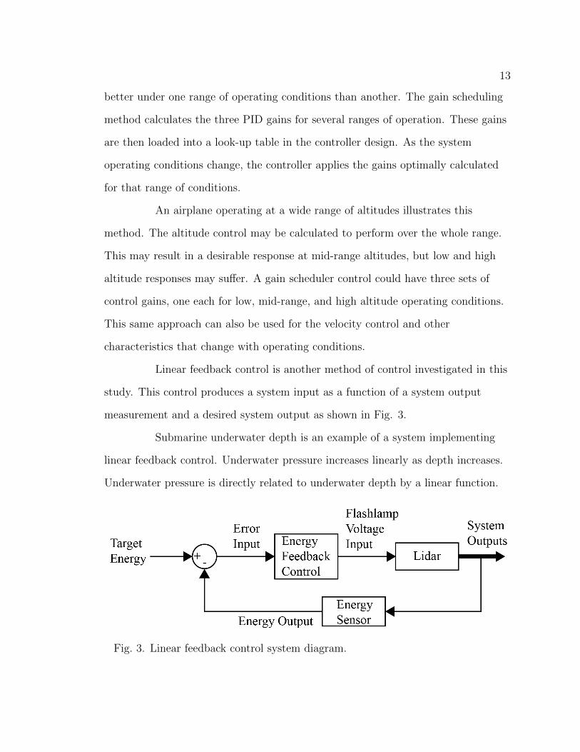
Linear feedback control is another method of control investigated in this
study. This control produces a system input as a function of a system output
measurement and a desired system output as shown in Fig. 3.
Submarine underwater depth is an example of a system implementing
linear feedback control. Underwater pressure increases linearly as depth increases.
Underwater pressure is directly related to underwater depth by a linear function.
Fig. 3. Linear feedback control system diagram.

14
This facilitates the implementation of a linear feedback control that will adjust the
system inputs to produce optimal performance at all depths.
For optimized computation, most dynamic systems utilize a real-time
operating system or a microcomputer enabling extensive control of the timing and
process allocation [52]. Even though a number of components in the lidar at CSUC
could benefit from a dynamic control, this study is focused on performance
stabilization, process synchronization, data acquisition, data transmission, and
communication.

CHAPTER III
HISTORY AND COMPONENTS OF
THE RAMAN-SHIFTED EYE-
SAFE AEROSOL LIDAR
History of the Raman-Shifted Eye-SafeAerosol Lidar
Prior to the Raman-shifted Eye-safe Aerosol Lidar (REAL), high
pulse-energy atmospheric lidars either presented ocular hazards or had limited
performance capabilities [53]. The REAL successfully produces, with an eye-safe
beam, high spatial and temporal resolution aerosol data with sufficient SNR to
reveal atmospheric structure up to ranges of 3 to 10 km depending on atmospheric
conditions.
The development of the REAL began in 2002 at the National Center for
Atmospheric Research (NCAR) in Boulder, Colorado [54]. Dr. Shane Mayor and
his group at NCAR were successful in creating an eye-safe lidar using SRS for
wavelength conversion. The REAL nominally transmits 170 mJ pulses at a 10 Hz
rate into the atmosphere. These parameters allow high spatial resolution scans to
be produced at 15 second intervals typically.
The first major experiment involving the REAL was the Pentagon Shield
field program in Washington, DC from April 9th to May 16th, 2004 [55]-[57]. The
REAL was deployed as a surveillance instrument to reveal otherwise undetectable
aerosol activity in the area. The experiment was successful, and in 2005 a
15

16
reproduction of the REAL was installed near the Pentagon and operated for over
eight years [58]-[60]. Unfortunately, the control system of the reproduction was a
proprietary component and the intellectual property was not shared for use in the
prototype instrument.
The same REAL used in the Pentagon Shield field program was deployed
in Dixon, CA, from March 15 to June 11, 2007 in the Canopy Horizontal Array
Turbulence Study (CHATS) [14]-[16]. The REAL operated almost continuously at
CHATS for three months and collected data that have been a subject of analysis
since. Data and experience gained during the experiment have been useful in the
continued refinement of the REAL.
Although the REAL has been deployed in multiple field experiments, the
Pentagon Shield field program and CHATS represent milestones in the development
of the instrument. The Pentagon Shield field program was the debut for the REAL
as a scanning, eye-safe, and high pulse-energy lidar and was the first opportunity to
demonstrate the capability in a dense urban environment. Similarly, CHATS was
the first long-term (3 months) experiment that captured data from both horizontal
and vertical scans of the atmosphere over an agricultural forest canopy. Within the
CHATS data, density current fronts have been discovered [61] and two dimensional
horizontal images of fine-scale canopy waves have been revealed [62]-[64].
In August 2008, the REAL arrived at California State University, Chico
(CSUC). With the support of three grants from the National Science Foundation
(NSF awards 0924407, 1104342, and 1228464), the REAL has been a source of
research opportunities for students and faculty from several departments. Projects
include analysis of fine-scale gravity waves, atmospheric boundary layer height
analysis, wind vector algorithm development, web application development, and
engineering projects [65].

17
Description of the Raman-ShiftedEye-Safe Aerosol Lidar as
Currently Configured
Lidar Transmitter
The transmitter of the lidar has three main components: (1) a 1 µm
wavelength, flashlamp-pumped, Nd:YAG laser; (2) a 1.5 µm wavelength seed laser;
(3) and a Raman cell that facilitates SRS of the 1 µm wavelength energy. Together,
the elements produce nominally 170 mJ pulses at a rate of 10 Hz at a wavelength of
1.5 µm. The beam is expanded to a 10 cm diameter before being projected into the
atmosphere [53]. At this energy density and wavelength, the instrument is eye-safe
according to the American National Standard Institute [66]. The Nd:YAG laser is a
Continuum Surelite III capable of producing 900 mJ pulses at 1.064 µm, a pulse
length of 6 to 9 ns, and a pulse rate of 10 Hz. The output energy of the laser can
be adjusted by the flashlamp voltage and the Q-switch delay either manually from
the front panel of the power and cooling unit (PCU) or remotely from a computer
to the PCU through an RS-232 connection. The flashlamp voltage input range is
1.47 to 1.57 kV in increments of 0.01 kV.
The wavelength converter, the Raman cell, is a cylindrical chamber 80
cm in length that is pressurized with 9.5 parts methane and 4.1 parts argon to 1379
kPa (200 psi) [67]. A folded cell geometry with prisms enables the Nd:YAG beam
to achieve a 3 meter interaction path length in the gas mixture. The Nd:YAG
beam excites the methane in the cell and the first-Stokes SRS re-emits energy at a
wavelength of 1.5 µm. The argon gas in the cell acts as a buffer gas to prevent
Raman scattering at higher-order Stokes and anti-Stokes lines which are not
necessarily in the eye-safe region of the spectrum and are capable of damaging

18
optics. Internal fans circulate the gas mixture to prevent thermal blooming from
compromising the beam quality of subsequent pulses.
The Raman cell is injection seeded with a ThorLABS
WDM8-C-33A-20-NM DFB laser that produces a continuous wave (cw) beam of 20
mW at 1.54373 µm. This beam is essential in the Raman-shifting process, as it
seeds the first-Stokes SRS process within the Raman cell. The seed laser improves
the conversion efficiency by stabilizing the Stokes output and improves beam
quality by reducing beam divergence [53], [57], [67]. The Nd:YAG laser can be
injection seeded as well to increase the conversion efficiency further [67]. However,
the system at CSUC does not currently contain such a feature.
Two beams exit the Raman cell: (1) the 1.5 µm wavelength, and (2) the
residual 1 µm beam. They are physically separated by a prism in order to block the
1 µm beam.. When optimized, the SRS process using an unseeded Nd:YAG beam
has a conversion efficiency near 30%. The nominal 170 mJ of 1.5 µm wavelength
energy is typically sufficient to generate good SNR at ranges of up to 3 to 5 km or
more, depending on atmospheric conditions and other aspects of instrument
performance. Other factors that affect instrument performance include, for
example, optical efficiency of the telescope and beam steering unit, alignment of the
transmit beam and receive field-of-view, and gain and noise levels in the detection
subsystem.
The optical components used in the 1 µm wavelength Nd:YAG beam
(before reaching the Raman cell) include a Faraday isolator, a beam reducer, and
25 and 50 mm diameter turning mirrors. The 1.5 µm seed laser beam uses a
collimator, isolator, half wave plate, and turning mirrors to co-align the seed laser
beam with the Nd:YAG beam before it enters the Raman cell. A short-wave-pass
dichroic mirror, pellin broca prism, holographic splitter, corner cube, and beam

19
block remove the excess 1.064 µm energy from the transmit beam. A beam
expander lowers the energy density of the 1.5 µm wavelength pulses to be eye-safe.
Turning mirrors direct the transmit beam into the atmosphere through the beam
steering unit (BSU). Two Molectron energy meters and a DataRay WinCamD
Beam Profiler monitor transmitter performance. A temperature sensor and
pressure sensor monitor the Raman cell.
Beam Steering Unit
The elevation over azimuth style BSU, designed and built at NCAR,
directs both the transmit beam and the receiver field of view in the atmosphere.
The BSU is a series of two Zerodur, gold-coated, light-weight mirrors on rotating
axes. Two Anamatic servo motors, SM2340D and SM3420D, rotate the azimuth
and elevation mirrors, respectively. The elevation motor receives power and
communication through a 16-channel slip-ring to facilitate continuous scanning in
one direction. Each mirror is designed to have a flatness of within 3 wavelengths
(0.9 µm of sag) across the full aperture [54]. The beam steering unit operates on a
control loop independent from the program being executed on the system PC. Once
issued a command, the BSU motors will repeat the command without further
communication with the lidar control program until another command is issued.
Receiver and Data Acquisition
The primary telescope mirror, 40.6 cm in diameter, collects backscatter
radiation and focuses it into a receiver subsystem [54]. The receiver is composed of
a collimating lens, a set of neutral density filters, an interference filter, a half-wave
plate, and a beam splitter. The beam splitter separates the two polarization
components of the backscattered radiation and each is focused on to a detector.
The detectors are InGaAs avalanche photodiodes (Perkin Elmer part number
C30659-1550-R2A). The InGaAs detectors [53] produce a voltage waveform

20
representing backscatter energy received as a function of time. The backscatter
energy waveform is amplified with an AD829 [37] and digitized by a National
Instruments (NI) PCI-5122 digitizer operating at 100 MS/s with a 14-bit
resolution. The digitizer is read by a LabVIEW program being executed on the
system PC, a Dell T7500 running a Windows 7 Professional 64-bit operating
system with an Intel(R) Xeon(R) E5620.
The REAL is connected to the network on the main campus by a 2 km
wireless connection to the CSUC Farm office and another 6 km wireless connection
to campus. The connection to the CSUC Farm office is a 36 Mb/s, 2-channel
connection. The bandwidth between the CSUC Farm office and the campus is 400
Mb/s.
Container and Environment
A custom-designed shipping container (6 x 2.5 x 2.5 meters) houses the
lidar on a flat-bed semi-truck trailer as shown in Fig. 4. Air conditioning units,
heating units, and insulation keep the container temperature-controlled
independent of instrument operation and a HEPA filter system purges the
transmitter subsystem with particle-free air. Temperature within the housing
container varies between 22 to 28 degrees Celsius. The optical components are
mounted on a 5-meter-long optics table. Interior environmental sensors include
temperature sensors, platform attitude sensors, a utility power sensor, and a
security system.
The lidar is located at the California State University, Chico (CSUC)
Farm, 3 km outside the city limits of Chico, California and 6 km from the CSUC
campus. The instrument is surrounded by fields of corn, alfalfa, sunflowers, and
almond orchards. The weather is similar to a typical Mediterranean climate - dry
and sunny from spring to the fall and rain in the winter.

21
Fig. 4. Photograph of lidar at the CSUC farm. The container on the left is used asa field office. The container on the right houses the lidar. The BSU is on the top ofthe right container.
LabVIEW Language and Signal Flow
The majority of the system that operates and controls the lidar is written
in LabVIEW, a graphical object language. National Instruments (NI) develops and
supports this language and hardware products that easily interface with LabVIEW
programs. The program used to operate the lidar implements a state machine that
executes a main loop upon receiving a trigger signal from the Nd:YAG laser.
The original LabVIEW program that controlled the REAL when it
arrived at CSUC was written by Mr. Bruce Morley at NCAR. It provided basic
ON/OFF capabilities for the instrument. This program was rewritten as this study
developed and new features were added. The resulting program uses many of the
same sub-programs while implementing multiple new control features, a
restructured state machine, and multiple redesigned processes. The REAL
LabVIEW program is detailed further in Appendix B.
CHAPTER IV
EXPERIMENTAL PROCEDURES,
FINDINGS, AND SOLUTIONS
The high pulse-energy atmospheric lidar at CSUC is a scientific
instrument used in meteorological research. The lidar provides detailed wind field
and atmospheric boundary layer measurements over several square kilometers. In
the system’s transmitter, a high pulse-energy 1 µm wavelength laser pulses at a
rate of 10 Hz. These pulses are coaligned with a seed laser through a pressurized
gas cylinder called a Raman cell. A portion of the 1 µm laser energy entering the
Raman cell is converted from the 1 µm wavelength to an eye-safe 1.5 µm wavelength
with an efficiency of about 30%. The residual 1 µm energy is separated from the
laser path before the 1.5 µm energy is expanded and projected into the atmosphere
by the beam steering unit (BSU). The backscatter radiation (which is extremely
low energy) is collected by a primary telescope mirror and directed toward two
avalanche photodiode detectors, each 200 µm in diameter, in the receiver
subsystem. The design, testing, and implementation of the control system for this
instrument required organizing dependencies between control loop frequencies,
variable characteristics, process execution, and operating system constraints.
The design presented in this study incorporates control system design
concepts applicable to systems with a process loop distinct from that of the control
loop. Every system design has a timing aspect that plays a vital role in the
effectiveness of the control. Although it is generally better to apply a control
22

23
sooner than later, the quality of the control depends on the data collected since the
application of the previous control. Just as the operating system is the brain, the
sensors are the fingers that sense instrument performance. Quality of operation
depends largely on analog-to-digital converters (ADC) that read sensors and
digital-to-analog converters (DAC) that apply controls.
The frequency at which system variables are sampled and controls
applied determines the design of the code layout and hardware that control the
instrument. System variable measurements are recorded and used to flag the
“safe-shutdown” and “contact personnel” features of the control system. The
voltage applied to the flashlamps pumping the Nd:YAG laser is stepped over time
in an effort to stabilize the transmit energy. Data quality is improved through a
redesign of the backscatter data normalization algorithm and the implementation
of a control that can utilize one of the digitizer resolution settings available for
reading the photo detectors.
System Variables
The high pulse-energy atmospheric lidar used for this study transmits
laser pulses at a wavelength that is obtained through a process known as
stimulated Raman scattering (SRS). This process introduces components into the
system than would otherwise not be present such as a Raman cell pressurized with
flammable gas. This, along with the high pulse-energy Nd:YAG laser, could
potentially cause failures that are hazardous to components in the system.
An image of the container housing the lidar is shown in Fig. 5 with the
locations of components and sensors as indicated. The optical table is similarly
illustrated in Fig. 6. All the sensors throughout the instrument are read by ADCs
and the measurements are input to the main program being executed on the

24
system PC in the housing container. The main program then executes the control
algorithm that produces system flags to shut down gracefully, contact personnel, or
adjust the flashlamp voltage to stabilize transmit energy as described in Fig. 7.
Herein, the term “vital signs” refers specifically to at least the following system
variables: Nd:YAG beam energy, transmit beam energy, wavelength conversion
efficiency, and transmit beam radius. Otherwise, the term “system variables” refers
to all variables used by the program operating the system. The location numbers in
Fig. 5 and 6 are described in Table 1 with vital signs indicated with a ?.
Most system variables are sampled at a rate of 10 Hz with each pulse
from the Nd:YAG laser. Samples are averaged over the period of time required to
make one cross-sectional scan of the atmosphere. Therefore, one set of system
variable measurements corresponds to one scan. These once-per-scan records are
created, but not used, by the control system. These records allow for trends and
correlations to be identified between system variables during post-operation
processing and analysis performed by operators. For example, a correlation could
be investigated between the temperature of the Nd:YAG laser cavity and the beam
energy or radius.

25
TABLE 1System Components and Corresponding Location
Numbers for Fig. 5 and 6
System Component Location NumberTransmitter optics table · · · · · · · · · · · · · · · · · 1Receiver optics table · · · · · · · · · · · · · · · · · · · 2?Energy meter for 1.064 µm beam · · · · · · · · · · · 3?Energy meter for 1.543 µm beam · · · · · · · · · · · 4Temperature sensor for housing container · · · · · · · 5Temperature sensor for optics table · · · · · · · · · · 6Nd:YAG laser head · · · · · · · · · · · · · · · · · · · 7Temperature sensor for Nd:YAG laser head · · · · · · 7Raman cell · · · · · · · · · · · · · · · · · · · · · · · · 8Temperature sensor for Raman cell · · · · · · · · · · · 8Pressure sensor for Raman cell · · · · · · · · · · · · · 9CCD camera to monitor ? beam radius and centroid
position of the transmit beam · · · · · · · · · · 10Precipitation sensor · · · · · · · · · · · · · · · · · · · 11Nd:YAG PCU - reads flashlamp count and flashlamp
voltage· · · · · · · · · · · · · · · · · · · · · · · 12Sensor for absolute platform attitude · · · · · · · · · · 13Sensor for utility power · · · · · · · · · · · · · · · · · 14InGaAs Detector Control Voltage · · · · · · · · · · · · 15InGaAs detectors · · · · · · · · · · · · · · · · · · · · 15Sensor for BSU direction/movement · · · · · · · · · · 16System PC - execute LabVIEW program, monitor
available disk space, and calculate ? Raman cellconversion efficiency· · · · · · · · · · · · · · · · 17
Launch mirror · · · · · · · · · · · · · · · · · · · · · · 18Primary mirror · · · · · · · · · · · · · · · · · · · · · · 19
A list of the system components with the corresponding location number for Fig.5 and 6. In some cases location number labels are used to represent multiplecomponents due to size and limited detail of figures.

26
Fig
.5.
(Col
orre
quir
ed.)
Cuta
way
ofa
solid-m
odel
ofth
elidar
syst
em.
Loca
tion
num
ber
lab
els
des
crib
edin
Tab
le1.

27
Fig
.6.
Dia
gram
ofco
mp
onen
tpla
cem
ent
onop
tics
table
.L
oca
tion
num
ber
lab
els
des
crib
edin
Tab
le1.

28
Fig
.7.
Con
trol
syst
emhar
dw
are
com
pon
ent
sign
alflow
dia
gram
.

29
Temperature Sensors
Sensors monitor the temperature of the interior of the housing container,
the optics table surface, the Nd:YAG laser head, and the exterior surface of the
Raman cell. Though extreme temperatures may cause or be symptoms of failures
in the system, even small variations in temperature do indeed affect the overall
performance of both the transmitter and the receiver. One hypothesis is that
temperature variation affects thermal lensing in the Nd:YAG rod that changes the
convergence and energy density and therefore conversion efficiency. In the receiver,
the InGaAs detector sensitivities also vary with temperature [37]. Three of the
sensors are K type thermocouples read by the National Instruments (NI) SC-2345
with three NI SCC-TC01 modules. The container temperature sensor is a pt 3750
type resistance temperature detector read by the NI SC-2345 with a NI
SCC-RTD01. The InGaAs detectors in the receiver also have a built-in temperature
sensing diode to adjust a bias voltage for stability in detector sensitivity.
Pressure Sensor
The Raman cell is pressurized with 9.5 parts methane (CH4) and 4.1
parts argon (Ar) to 1310–1448 kPa. A decrease in pressure will affect the
wavelength conversion efficiency and result in a decrease in transmit energy [53]. A
sudden decrease in pressure from a leak in the Raman cell will cause the release of
the flammable gas into the instrument housing container. The pressure is measured
using an Ashcroft 2F249 pressure transducer which is read by the NI SC-2345 with
a NI SCC-FT01 module. The SCC-FT01 measures the voltage drop created as the
4–20 mA output of the transducer passes through an external 249 ohm resistor.

30
Energy Meters
Two pyroelectric Molectron energy meters quantify the total energy in
each pulse just before entering the Raman cell and again after exiting the Raman
cell. Before the Raman cell, the total energy of the 1 µm Nd:YAG pulse is
measured. After the Raman cell, the total energy of the 1.5 µm transmit pulse is
measured. The efficiency of the stimulated Raman scattering in converting the
wavelength of the pulse in the Raman cell is a key indicator of system performance.
These two energy readings are used to calculate this conversion efficiency.
conversion efficiency percentage =Energy at 1.543 µm
Energy at 1.064 µm× 100 (1)
Flashlamp Pulse Count and Voltage
The Nd:YAG Continuum Surelite III laser includes a head unit with a
power and cooling unit (PCU) that are located approximately 5 m apart on the
optics table. The PCU and laser head are connected by water lines, power cables,
and control cables, each approximately 7 m in length. The main LabVIEW control
program interfaces with the PCU via RS-232. The two commands that are used
most frequently are a flashlamp pulse count read and a flashlamp voltage write.
Other commands check for errors, turn the flashlamps ON or OFF, turn the laser
head shutter ON or OFF, adjust the Q-switch delay (pulse-energy), adjust the
pulse rate, and open or close the communication port.
The flashlamp pulse count command returns the number of pulses the
Nd:YAG laser has discharged in its lifetime. This metric is used in the transmit
energy control algorithm. At the beginning of this study the unit’s pulse count was
86 million. The flashlamp count is determined by subtracting the number of pulses
on the unit when the present flashlamps were installed. The flashlamp voltage is

31
the output of the laser energy control algorithm. This voltage is written to the unit
on startup and during operation once per scan.
Beam Steering Unit Direction andMovement Sensors
The elevation over azimuth style beam steering unit (BSU) operates on a
control loop independent from the main system. At the beginning of operation, the
BSU receives a command that is stored within the BSU motor onboard computers
and repeatedly executed until a different command is issued. A command is
generally a scan sequence such as: (1) initial azimuth and elevation angles, (2) a
scan rate, (3) final azimuth or elevation angle for horizontal or vertical scans,
respectively, then (4) a reset to the initial angles. Two Anamatic servo motors,
SM2340D and SM3420D, rotate the azimuth and elevation mirrors, respectively. If
the power to the motors is interrupted, the motors will stop and require a
reinitialization before continuing. Reinitialization is required for correct azimuth
and elevation axis orientation. Power and communication to the BSU motor
controlling elevation are delivered through a 16-channel slip ring to enable
continuous scanning in one direction. The BSU is bolted to a large tip-tilt stage
attached to a tower made of 80/20 extruded aluminum. This tower is fastened to
the transmitter/receiver optics table so that the BSU and optics table form a
monolithic structure independent of the housing container.
Prior to this research, the encoders built into the BSU motors were
determined to be insufficiently accurate. Angular decoders were installed that
produce measurements with 10−4 of a degree precision. The decoders are read by
the NI SC-2345 through digital counter ports. These high precision decoders allow
for a more accurate and reliable measuring of the BSU direction. However, due to
the nature of scan sequence types and timing, the control algorithms for the BSU

32
are limited. For example, a new scan is defined as the moment the current BSU
angle is greater than the previous angle. The scan has ended when the current
angle is less than the previous angle. This assumes that the lidar will always scan
in the same direction, which is true as currently configured. A freeze (failure caused
by momentary loss of power) is defined to be true after a pre-determined number of
seconds pass without the start of a new scan. A future feature will include a timed
scan interval in which each scan will commence after a operator-defined interval of
time greater than the length of the scan. This will be done by recognizing that a
scan has been completed and commanding the BSU to return to point in the start
direction and hold. The moment the scan interval has elapsed, the program will
issue a command to the BSU to begin scanning again. This feature is needed to
produce scans and wind measurements at consistent, operator-defined intervals,
and to coordinate scans with other lidar systems in field research.
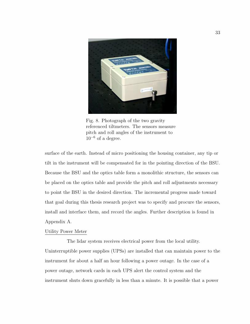
Absolute Attitude Sensors
The high pulse-energy atmospheric lidar can collect backscatter signal
from ranges of more than 10 kilometers. Any pitch or roll movements in the
housing of the instrument will result in a beam displacement in the atmosphere.
Two Applied Geomechanics Model 801 Tuff Tilt Uniaxial Tiltmeters are used to
monitor the pitch and roll of the instrument. Each tiltmeter has an angular range
of ±0.5 degrees and a resolution of 10−6 degrees. These gravity-referenced
electrolytic tilt transducers produce a voltage read by the NI SC-2345 using a NI
SCC-FT01. A photograph of the two tiltmeters is shown in Fig. 8.
The longer-term goal for these devices is to use them for precise laser
beam positioning at far ranges. Pitch and roll measurements will be used to adjust
BSU elevation angle just before each laser pulse to compensate for movement in the
instrument and maintain precise control of the altitude of the beam above the
33
Fig. 8. Photograph of the two gravityreferenced tiltmeters. The sensors measurepitch and roll angles of the instrument to10−6 of a degree.
surface of the earth. Instead of micro positioning the housing container, any tip or
tilt in the instrument will be compensated for in the pointing direction of the BSU.
Because the BSU and the optics table form a monolithic structure, the sensors can
be placed on the optics table and provide the pitch and roll adjustments necessary
to point the BSU in the desired direction. The incremental progress made toward
that goal during this thesis research project was to specify and procure the sensors,
install and interface them, and record the angles. Further description is found in
Appendix A.
Utility Power Meter
The lidar system receives electrical power from the local utility.
Uninterruptible power supplies (UPSs) are installed that can maintain power to the
instrument for about a half an hour following a power outage. In the case of a
power outage, network cards in each UPS alert the control system and the
instrument shuts down gracefully in less than a minute. It is possible that a power

34
outage could prevent communication with personnel through the Ethernet network
connection. The security system, which can operate by battery for days, has a
feature that uses GPRS (cellphone) communication channels to contact personnel
in the event of a power outage.
Disk Space Meter
The computer executing the control system program has two physically
independent 2 terabyte hard disk drives for storage of the backscatter data. The
files on each disk are duplicates (RAID 1) for safety. The available disk space is
monitored and personnel are notified or the system is shut down if the available
space is less than a predetermined threshold. Disk space usage rate depends on the
resolution and range of data being saved. Two terabytes of data (saving data to 5.8
km range at 1.5 meters per gate at 10 Hz) will be recorded after three months of
continuous operation which corresponds to three sets of flashlamps.
Precipitation Sensor
Operation of the lidar is not optimal when precipitation is falling.
Precipitation attenuates the transmitted pulses and backscatter radiation which
significantly limits the range of useful data. In addition, the BSU azimuth motor is
more exposed to precipitation when the BSU is scanning the atmosphere, and water
drops on the face of the protective glass BSU window cause unwanted backscatter
of the transmit beam and obstruct the receiver field of view. Therefore, a Thies
Clima 5.4103.10.700 precipitation monitor detects hydrometers and flags the
control system to enter a sleep mode. This sensor activates a relay when 1 to 15
drop incidences are detected and switches back 25 to 375 seconds after the last drop
incidence, as set by the operator. The precipitation sleep mode stops operation,
stows the BSU into a protective posture covering the azimuth motor, and allows

35
Fig. 9. Photograph of the precipitationsensor. The system enters a sleep modewhen the precipitation sensor detects rain.
the system to sleep and then wake to continue operation after precipitation has
stopped. A photograph of the precipitation monitor is shown in Fig. 9.
Beam Profiler
The Nd:YAG laser beam profile is monitored constantly with a DataRay
WinCamD-UCD12. This sensor is a CCD camera that, with the DataRay software,
can display the laser beam cross-section. The profiler is interfaced into the control
system and drivers are used to extract three variables from the camera: centroid’s
X location and Y location, and beam radius. These measurements are made from
the raster image produced by the CCD camera and an algorithm on board the
camera’s computer. The DataRay software shows high beam energy density as
warm colors (i.e., white, red) and low energy density as cool colors (i.e., blue,
green). Centroid location is determined to be the center of total energy density.
The beam radius is measured at the 1e2
level as for a Gaussian beam profile. Power
and communication are delivered via USB. The device is not fast enough to capture
each pulse at 10 Hz and therefore measurements may be held for two to three pulses

36
Fig. 10. Photograph of the DataRay WinCamD beamprofiler in the transmitter of the instrument. The pellinbroca prism that directs a sample of the Nd:YAG laserbeam to the CCD camera is shown on the right side of thephotograph.
before a new measurement is made. A photograph of the CCD camera is shown in
Fig. 10 and Fig. 11 shows an example of the raster image produced by the sensor.

37
Fig. 11. (Color required.) Typical beamprofile produced by the DataRay WinCamDCCD camera. The cross-section shows thecenter of the beam to have a high energydensity with the centroid indicated by theintersection of the two lines.
InGaAs Detector Control Voltage
The parallel and perpendicular polarized components of the
backscattered radiation are focused onto two Perkin-Elmer C30659-1550-R2A
InGaAs Avalanche Photodiode Detectors in the receiver subsystem. This compact
detector has an active area of 0.03 mm2. The detector has a pre-amplifier and a
temperature diode that is used to control the bias voltage that regulates detector
sensitivity. The temperature diodes are monitored by the NI SC-2345 using two NI
SCC-FT01 modules. The input is processed and bias voltages are driven using
another pair of NI SCC-FT01 modules. The output waveforms of the detectors

38
each pass through a post-amplifier before being read by the NI PCI-6229 high
speed digitizer.
Laser Energy Control
During the Canopy Horizontal Array Turbulence Study (CHATS)
experiment of 2007 the flashlamp voltage was increased manually with computer
every week or so and could not be changed unless the system was stopped. Truly
continuous operation requires that the voltage be changed without interrupting
data collection. Unattended operation requires that this change be made without
the assistance of an operator. When this requirement is met, the constraint on
continuous operating time is the life of the flashlamps, between 23 and 34 days of
round-the-clock operation. A trained person may change the flashlamps in less
than 30 minutes.
Vital sign and system temperature data from the CHATS experiment are
displayed in Fig. 12 [68]. Notice the transmit (SRS) energy at 1.5 µm on the lower
graph has a sawtooth pattern. The steady increase in beam size and decrease in
transmit energy is due to the aging of the flashlamps in the Nd:YAG laser. After
the transmit energy has decreased by some amount, an operator manually
incremented the flashlamp voltage in an effort to increase the transmit energy back
to the original level.
Manual voltage adjustment during the experiment was inconsistent with
varying increment size and interval. The voltage increment range is between 1.47
and 1.57 kV with minimum increments of 0.01 kV. This represents 11 available
voltage settings for the lifetime of a set of flashlamps. According to the CHATS
record, which spans the life of three sets of flashlamps, the voltage would have had
to be adjusted 4 or 5 times during the life of a flashlamp set as indicated by the

39
Fig. 12. (Color required.) Time-series of several vital signs during the 2007 CHATSexperiment. This experiment was performed from March 19 to June 11, 2007 withno control system. The X-axis units are Julian days of the year 2007. Thesawtooth shape of the transmitted (SRS) energy (bottom plot) is a result of agingof the flashlamps and manually increasing the flashlamp voltage periodically.
steps in the bottom plot of Fig. 12. Sometimes the voltage was increased by just
0.01 kV and other times by 0.02 kV. This does not take full advantage of the 11
flashlamp voltage settings available. This study identified two methods of flashlamp
voltage control: a linear feedback method and a gain scheduler method.
The linear energy feedback control is designed to stabilize the laser beam
energy by adjusting the voltage regardless of the increment size and interval
required. In other words, stabilization can be achieved by changing the voltage by
any amount as frequently as needed. In contrast, the gain scheduler control is

40
designed to change the voltage at fixed increments and time intervals regardless of
whether the laser energy is at the desired level or not.
Linear Energy Feedback Control
The linear energy feedback control was the first control method
investigated in this research. This control type uses operator-set transmit energy
level thresholds to trigger incremental increases in the flashlamp voltage as the
average transmit energy decreases with time. The feedback control is designed to
produce an optimal laser energy over the life of the flashlamps. The feedback
control may or may not use all 11 flashlamp voltage settings and it may or may not
adjust the voltage at equal intervals. This method is designed to keep the energy at
or above a operator-specified value. This method is designed to produce a beam
energy that is constant over the lifetime of the flashlamps.
A critical piece of the design of the linear feedback control method is the
operator-defined energy threshold, shown as the input in Fig. 13, that triggers the
voltage incrementation. If the energy threshold is too low, the voltage will not
optimally use all 11 values of incrementation that are available and will therefore
produce a lower transmit energy of the life of the flashlamps. At the end of their
lifetime, the flashlamps would theoretically have “life” remaining. However, if the
energy threshold is too high, the voltage will increment too quickly and use all 11
values of incrementation before appropriate for the age of the flashlamps. At best,
this would produce a higher transmit energy over the life of the flashlamps but
exhaust their range of control quickly. At worst, the voltage would increase faster
than the flashlamps are designed to operate, thus shortening their lifetime. Limits
might need to be enforced on the control voltage to prevent a “run-away” voltage.
This method also assumes that the pulse-energy decreases linearly over
the lifetime of a flashlamp set. This is a theory that has not yet been confirmed. If

41
Fig. 13. Lidar control system diagram with energy feedback loop.
the theory is wrong and the beam energy decreases non-linearly then a constant
energy threshold may not be appropriate. Such a non-linear feature in the system
would require a more complicated algorithm. A flashlamp voltage experiment was
devised to study the effect this control system might have on the performance of
the instrument.
Flashlamp Voltage Experiment
To study how the flashlamp voltage affects the performance of the
instrument, an experiment was conducted. For 1 hour the system was operated for
5 minutes at each of the 11 flashlamp voltage settings with less than 2 minutes of
rest between each interval. During the 2 minutes of rest, the flashlamps were not
pulsing while the voltage was being adjusted. Performance was recorded and three
variables are displayed in Fig. 14. A photograph of the flashlamps discharging in
the laser head cavity is shown in Fig. 15.
The 1 µm Nd:YAG laser energy (top, Fig. 14) increases in a step-like
fashion but both the transmit energy (middle, Fig. 14) and the conversion
efficiency (bottom, Fig. 14) increase steadily and then level off about halfway
through the experiment. Toward the end of the experiment even a slight decrease
was noted in the trend of each variable. After completion of this experiment it was

42
Fig. 14. Time vs. laser energy and conversion efficiency during the 11increments of the flashlamp voltage. The system was operated forapproximately five minute periods at each of the 11 flashlamp voltage levelsbeginning with 6,393,146 pulses on the flashlamps. This was a study of theeffect of the flashlamp voltage on the vital signs of the instrument.
concluded that the system should be operated at the flashlamp voltage
corresponding to the maximum conversion efficiency, about 1.55 kV. This voltage
represents the voltage that the linear energy feedback control would determine
appropriate to maximize transmit energy. Prior to this experiment, the flashlamp
voltage was set to 1.47 kV for the current flashlamps.
At this point it is noted that the manual for this Nd:YAG laser indicates
that a flashlamp set may be used for 20 to 30 million pulses. The pulse count for
the beginning of this experiment was 6,393,146 pulses which represents between
21-32% of the lifetime of the flashlamp set. If the voltage increments were

43
Fig. 15. Photograph of the flashlamps discharging in theNd:YAG laser cavity.
distributed over the lifetime of the flashlamps evenly, the 6,393,146 pulse count
would correspond to a setting between 1.49 and 1.51 kV.
The instrument was operated for a 10-hour day with the flashlamp
voltage set at 1.55 kV and then shut down by the operator. The next morning the
instrument was restarted. After one and a half hours a failure occurred.
Fortunately, a section of the fail-safe feature of the control system (discussed in the
next section of this chapter) was already implemented and it detected the failure
which manifested as a sudden decrease in transmit energy. The fail-safe feature
shut the instrument down quickly (after 500 ms or 5 pulses) and gracefully before
the failure could affect other components of the system.
Investigation revealed that one of the four prisms in the Raman cell had
been damaged. It was hypothesized the prism may have been damaged by an
increase in energy density in the beam through the Raman cell. An experiment was
devised to validate this theory.

44
Beam Conversion Through RamanCell Experiment
At the time of the failure of the Raman cell prism, there were 10,779,826
pulses on the flashlamps. Again, it is noted that this corresponds to 36 to 54% of
the life of a flashlamp set. Also, if the voltage increments were distributed over the
lifetime of the flashlamps evenly, the 10,779,826 pulse count would correspond to a
setting between 1.50 and 1.53 kV.
Fig. 16. Photograph of the damaged Raman cellprism.
After removing and repairing the Raman cell, data analysis was
performed to estimate the 1 µm wavelength energy density through the Raman cell.
It was expected that increasing the flashlamp voltage moved the waist of the beam
from beyond the Raman cell where it should be, to inside the Raman cell. If this
expectation were true, the waist, being the point of smallest beam cross-section and

45
thus highest energy density, could have been located on or near a prism and caused
the damage.
The system is designed with the waist of the beam beyond the Raman
cell because, although high energy densities improve wavelength conversion
efficiency, the waist of the beam may have high enough energy density to optically
break down the gas and cause sooting [69], [70]. A slight convergence of the beam
through the cell provides optimal conversion efficiency while preventing damage to
the optics.
The beam energy density through the Raman cell was measured using
laser burn paper to measure the beam radius at 20 cm increments for 3 meters
starting from the position of the entrance window of the Raman cell. This length
represents the path length of the beam folded in the Raman cell. Fig. 17 displays
the results of the experiment. The images in Fig. 17 are a negative color
representation of what appears on the burn paper for clarity in print. The burn
paper is actually black and burn spots are white and yellow.
Several characteristics of the beam are identified in this experiment by
visual inspection of the burn paper. The first is that the overall shape of the beam
profile changes with an increase in either distance or voltage. The beam profile
starts as an oval shape and changes to the diamond-star shape with four distinct
corners. The measurement at 180 cm with a voltage of 1.55 kV was erroneous and
therefore, was omitted from the figure, and was interpolated based on neighboring
data points. Conversion trends are readily apparent as the voltage and distance
increase.

46
Fig. 17. (Color required.) Color negative burn paper results fromflashlamp voltage vs. conversion experiment. ZAP-IT laseralignment paper was set at distances between 20 and 300 cm, atincrements of 20 cm, from the mirror that turns the beam into theRaman cell. This was repeated for each of the 11 flashlamp voltagesettings available to measure beam energy density, beam waistmovement, and beam profile shape through the Raman cell vs.flashlamp voltage.

47
Fig. 18. (Color required.) Energy density of the Nd:YAG beam at 1 µm vs.distance from the Raman cell entry window per flashlamp voltage. The trianglesrepresent the actual peaks of those curves. The peaks represent the highestenergy density in the beam, also referred to as “the waist.” The vertical dashedlines indicate the approximate locations of the Raman cell prisms. The thickervertical dashed line represents the approximate location of the Raman cell prismthat was damaged. Notice that the curves corresponding to flashlamp voltages1.52 to 1.57 kV have peaks within Raman cell.
A Java-based computer program, ImageJ, was used to measure the area
of the beam’s centroid. The burn paper was scanned into a computer at 1200 dpi.
ImageJ was used to find the area in pixels of the centroid of each pulse. The
centroid was taken to be the area inside the ring that was most distinct. Because
burn paper is an uncalibrated measurement media, exact energy density is
approximated using the energy levels of the flashlamp voltage experiment as shown
in Fig. 14.

48
The results of the experiment are revealed in Fig. 18 with dashed
vertical lines marking the approximate positions of the four prisms inside the
Raman Cell. The bold line represents the prism that was damaged. Maxima in the
energy density are marked with 4. Note that the maxima for each curve represent
a waist in the beam and a peak in energy density. For low voltages the waist is
located beyond the exit window of the Raman cell (a distance of three meters from
the entrance window) as expected. As the voltage is increased the waist moves into
the Raman cell and may result in energy densities that are higher than the damage
threshold of the optics. As expected, the voltages that produce a beam with a
waist inside the Raman cell are voltages 1.52 to 1.57 kV as identified with the 4.
This experiment confirmed the theory that prematurely increasing the
flashlamp voltage moves the beam waist from beyond the Raman cell to inside thus
increasing beam energy density above the damage threshold of the optics. The
linear energy feedback control does not, therefore, have all 11 flashlamp voltage
settings available at all times. The control would need to know the location of the
waist which is not possible with the present configuration of the instrument.
This experiment concluded that the linear energy feedback control has
limited capabilities in stabilizing the transmit energy and introduces high energy
density risks to the wavelength converting part of the instrument. It was decided
that the gain scheduler control would be investigated as a solution that would
provide more stable transmit energy.
Gain Scheduler Control
The gain scheduler method implements a look-up table (LUT) to set the
flashlamp voltage based on the number of flashlamp discharges. The LUT is
designed to take advantage of the full range of voltage settings, incrementing ten
times in the life of the flashlamps at even intervals. The gain scheduler system

49
(a) Lidar control system diagram with pulse count feedbackcontroller.
(b) Pulse count feedback controller implemented as a look-uptable (LUT).
Fig. 19. Lidar control system diagram with pulse countfeedback controller. The pulse count feedback controller isimplemented as a look-up table (LUT). This was the controlimplemented for the field experiment performed in this study.

50
diagram and LUT are shown in Fig. 19. The beam energy may decrease or increase
over the lifetime of a flashlamp set but should be more uniform and consistent. The
flashlamp voltage will increase every two to three million pulses depending on the
expected flashlamp lifetime of 20 or 30 million pulses, respectively.
An experiment was performed to collect new data that were compared
with the data from the CHATS experiment (Fig. 12). The lidar was operated
continuously and unattended from October 2 to October 22, 2012. On October 22,
a rain storm interrupted the experiment but operation resumed on October 25 and
continued through October 30. The flashlamp voltage was adjusted according to a
20 million pulse lifetime. The results are shown in Fig. 20.
By comparing Fig. 12 with Fig. 20, several differences can be observed.
It is important to note the scale of the vertical axis on the plots. The main goal in
this experiment was to stabilize the Nd:YAG energy. A scaled comparison of the
Nd:YAG beam energy and the transmit beam energy is shown in Fig. 21.
In Fig. 20 it was expected that the flashlamp voltage would have a
considerable effect on the beam energy and the SRS conversion efficiency and it
did. However, the goal was to stabilize the transmit power so that it does not
decrease over time with the aging of the flashlamps. It actually increased which
means the lidar will produce even better measurements over time. Experiments will
be performed in the future to investigate how transmit pulses from the early life of
the flashlamps might have energy levels similar to pulses from the later life of the
flashlamps. It is possible that the cause of this increase in energy is the result of a
flashlamp voltage incrementation schedule calculated for a 20 million pulse lifetime.
An incrementation calculated for a 30 million pulse lifetime might produce a
transmit energy more constant over the flashlamp lifetime. However, this energy
level would be closer to the starting energy level which is lower than the energy

51
Fig
.20
.(C
olor
requir
ed.)
Vit
alsi
gns
duri
ng
the
Oct
ober
2012
exp
erim
ent
usi
ng
the
gain
sched
uling
contr
olle
rw
ith
puls
eco
unt
feed
bac
k.
Ast
rong
corr
elat
ion
bet
wee
nte
mp
erat
ure
and
lase
rb
eam
ener
gyan
dra
diu
sis
not
ed.
Bot
hth
eN
d:Y
AG
and
the
tran
smit
bea
men
ergi
esw
ere
not
edto
hav
ean
incr
easi
ng
tren
das
the
flas
hla
mp
volt
age
incr
ease
s.

52
levels toward the end of the experiment. This is because flashlamp voltage
incrementation rate would be more proportional to the deterioration rate of the
flashlamp cathodes.
The 1.5 µm beam radius was monitored closely during the experiment.
The slight increase in radius toward the end of the experiment suggests that the
waist is moving farther from the exit window of the Raman cell as the flashlamps
age. Because beam energy density is increasing while the radius is decreasing,
energy density, and therefore conversion efficiency, remain more stable.
System temperatures are highly correlated with both beam energies, and
therefore, with conversion efficiency and the beam radius. A strong dependency on
temperature was not expected, but was found. It is hypothesized that the vital
signs are more sensitive to temperature than expected through the effects of
thermal lensing. The Nd:YAG rod used in this study is relatively long and
manifests thermal lensing as the rod is heated more on the axis of the beam than
on the outer regions. This temperature variation in the rod causes some transverse
gradient of the refractive index of the rod. Temperature variations in the laser head
accentuate this effect. Thermal lensing alters the intended convergence of the beam
thus affecting the vital signs of the instrument.
This finding will lead to further experiments to study the effect of
temperature and how it can be controlled to produce more stable results of the
instrument. The Nd:YAG rod temperature is stabilized using circulating water. A
future experiment might provide a larger reservoir of circulatory water thus
increasing the thermal mass and the temperature stability of the laser head. The
current reservoir is approximately one liter in size.

53
(a) Nd:YAG and transmit beam energies from the CHATS experiment
(b) Nd:YAG and transmit beam energies from the field experiment with flashlampvoltage control
Fig. 21. A comparison of data from the CHATS experiment (upper two plots,a) and the field experiment with flashlamp voltage control (lower two plots,b). The control designed in this study was tested on a new set of flashlampsto verify the effect on the beam energy over the lifetime of the set. Thiscomparison verifies the ability of the control to stabilize the beam energy.

54
Safe-Shutdown Feature
Prior to this study, unattended operation of the original REAL required
accepting the risk that a problem would go undetected and might initiate a chain
reaction of costly additional component failures and data loss. To reduce this risk
associated with long-term unattended operation, a safe-shutdown (or “fail-safe”)
feature was added to the control system. A fail-safe feature significantly reduces
the risk of catastrophic failures or data loss because out-of-range variables are
immediately detected and actions automatically taken to trigger a graceful
shutdown of the entire system.
The backbone of the safe-shutdown feature is a collection of thresholds
that will set a flag when violated by a measurement of the appropriate system
variable. Each variable in the system has at least one set of thresholds that acts as
a preventative measure against failures and damage to system components by
notifying personnel of system status and/or gracefully shutting down the
instrument. The threshold values are derived using component specifications and
data records.
The procedure for shutting down the system starts by closing a safety
shutter at the entrance to the receiver box, thus preventing any radiation from
reaching the InGaAs detectors, which are the most vulnerable components in the
system. At the same time the safety shutter is closed, a command is sent to the
Nd:YAG laser PCU to stop the flashlamps. Stopping the flashlamps prevents
further damage to system components that might have been caused by the
Nd:YAG laser, the most powerful component. The rest of the shutdown procedure
involves contacting personnel, closing communication ports, moving the BSU into
the stow posture, and cooling the laser head.

55
Nd:YAG PCU Key Turnerand Safety Shutter
An underlying goal of this research was to enable the lidar to operate
remotely using a connection from the main campus. Two obstacles that were
overcome were remotely powering on the Nd:YAG laser PCU and protecting the
InGaAs detectors. Dr. Eric Ayars from the Department of Physics at CSUC
designed and fabricated a microcontroller that activates a servo motor. The key
turner is a LabVIEW controlled servo motor and controller secured to the face of
the Nd:YAG laser PCU. When activated, this servo motor turns the power key to
the ON position. The key turner allows for remote control of laser power without
altering the existing equipment. A photograph of the key tuner is shown in Fig. 22.
Fig. 22. Photograph of Nd:YAG laser PCU power key turner.A microcontroller with a servo motor facilitates remoteoperation of the lidar.

56
Fig. 23. Photograph of the receiver boxsafety shutter. A microcontroller with aservo motor facilitates remote protectionof the InGaAs photo detectors.
The safety shutter is another servo with a controller and a matte black,
rigid, and light-weight card attached to the head. When activated, the card swings
down to block any backscatter radiation from entering the receiver box. The safety
shutter is shown in Fig. 23 in the position that blocks backscatter radiation from
entering the receiver box. The safety shutter provides remote-controlled protection
for the most sensitive components of the system.
These devices, along with network controlled uninterruptible power
supplies (UPSs) and power distribution units (PDUs), enable complete remote
operation of the instrument. This is done across a wireless network connection from
the lidar facility to the CSUC Farm office. Security cameras also assist by allowing
operators to view various components and conditions during remote operation.

57
Contact Personnel Feature
It is convenient to contact personnel as soon as a system variable exceeds
a preset threshold. Doing so enables engineers and operators to investigate and
take corrective action if necessary. Variables that are out of normal range trigger
warning or shutdown procedures that contact personnel via SMTP. Messages sent
to personnel include: (1) the name of the system variable that triggered the flag,
(2) the value of that variable, (3) the threshold the variable violated, and (4) the
time the event occurred. Messages are sent in the form of emails or text messages
to mobile phones. These text messages have been the quickest method of
communication. Currently, it is programmed to send an email to two addresses or
phone numbers. Personnel can respond to the messages and failures by logging on
to the system PC remotely through the network or traveling to the instrument to
adjust system components, perform maintenance, perform necessary repairs, or
simply restart the system.
There is one known risk in this design: messages are dependent on a
two-kilometer wireless signal from the lidar facility to the CSUC Farm office and
another from the Farm office to the main campus before accessing the Internet. If a
network failure occurred during unattended operation and personnel was not made
aware, the instrument would still be shut down gracefully. The system could
potentially be inactive for hours or days before personnel became aware of the
change, resulting in loss of time and data. This can be prevented by operators
simply checking a web application that posts the most recent system variable
measurements. If the data on the web application is not current and a message has
not been received, a system failure has occurred, the instrument has safely shut
down, and the network was not able to deliver the message to the operator.

58
Frequency of Control
A vital piece of the control design is the frequency at which it performs.
The Nd:YAG laser, pulsing at a frequency of 10 Hz, is not controlled by the main
program. The command to start lasing is issued by the main program and the laser
begins pulsing at 10 Hz independent of the control loop. Much of the preliminary
work on the control design was deciding whether to control at a faster rate, a
slower rate, or the same rate as the firing of the laser. After some research it was
apparent that a control loop that executed at any rate other than the 10 Hz of the
laser would unnecessarily introduce significantly more complexity to the system.
A slower control loop would likely occur once per scan of the atmosphere
and the control frequency would, therefore, depend on the duration of a scan.
When a scan is complete, the BSU returns quickly to the azimuth and elevation
angles that were specified for the beginning of the scan. During this time,
sometimes referred to as the “fly-back”, the transmitter will continue to pulse, but
backscatter data will not be recorded. The time the fly-back takes to occur is
usually between 400 to 800 ms depending on the angular width of scan. The 100
ms period of the Nd:YAG laser loop might constrain calculations that would be
possible during the fly-back time. If the control loop is executed faster than once
per scan it will happen inbetween laser pulses that need to be recorded. This limits
the control to what can be executed within the 100 ms period. If the control is
designed to execute more frequently than once per scan it might as well execute
every time the Nd:YAG laser pulses.
A control frequency of once per scan would be less computationally
demanding, but the control would not be fast enough to catch all failure cases in an
appropriate amount of time. For example, if the energy density in the Raman cell

59
exceeds damage thresholds, an immediate shutdown should occur. Data analysis
indicated that the 10 Hz control loop detected the drop in energy associated with
the damaged prism and shut down the system within 500 ms or 5 laser pulses. If
the control executed once per scan and the scan at the moment of energy density
increase was a wide, slow horizontal scan, it is possible that the scan could last up
to a minute. This is enough time to allow hot spots in the beam to begin damaging
other components.
In researching methods of timing control, National Instruments support
network was contacted. One of their suggestions included a master/slave
architecture. A master/slave architecture configures the 10 Hz Nd:YAG laser pulse
loop as the master loop that would execute the control loop, acting as the slave, as
often as possible. The slave loop executes independently of the master loop at a
rate that could be slower than 10 Hz, but it is as fast as the system PC will allow.
Because the slave loop executes independently, the master loop will record the
backscatter data for each pulse to prevent data loss. This would be an excellent
solution if the control could not execute within the 100 ms period of the master
loop. However, because the control can execute within the 100 ms period it was
decided to execute the control at least once per pulse to take advantage of some
additional capabilities of this method.
If the control loop executes at least once in the 100 ms period between
Nd:YAG laser pulses, one set of measurements could be collected from the system
variables for each laser pulse. This has proven essential for diagnosing a failure in
post-operation data analysis. In the case of the energy density increase in the
Raman cell that resulted in damage to a prism, data from the last three pulses were
used to identify the possible causes of the failure.

60
TABLE 2System Variable Measurements Distinguished by
Dependency on Nd:YAG Laser Pulse
System variable measurementsdependent on a Nd:YAG laser pulse
System variable measurementsindependent of Nd:YAG laser
?Nd:YAG laser beam energy Housing temperature?Transmit beam energy Optic table temperature?Raman cell conversion efficiency Raman cell temperature?Transmit beam radius Nd:YAG laser cavity temperatureTransmit beam centroid X location Raman cell pressureTransmit beam centroid Y location Precipitation sensorFlashlamp count Absolute attitude of platformFlashlamp control voltage Utility powerInGaAs Detector Control Voltage BSU pointing direction
BSU movementDisk space availability
The system variable measurements that are dependent on the Nd:YAG laserpulse cannot be used in a control frequency faster than the pulse rate of thelaser. Relatively few variables are left if such a controller is implemented.Vital signs are marked with a ?.
A faster control loop would significantly complicate the main program
code of the system. This type of design was considered until the role of the system
variables was investigated. Table 2 lists the system variable measurements that are
dependent on and independent of the Nd:YAG laser pulse with the vital signs
marked with a ?.
This analysis revealed that all vital sign measurements require the
discharge of the Nd:YAG laser. Then the question became “Is a frequency of 10 Hz
adequate to control all variables?” Each system variable has a different rate of
change. Temperature in the housing container, for example, will not change faster
than about three degrees Celsius per minute. Beam energy, however, could drop
dramatically from one pulse to the next if, for example, an optic is damaged.

61
Analysis revealed that no system variable could be controlled fast enough to
prevent a failure from developing between the 10 Hz pulses.
Along with the rate at which system variables change, the rate at which
sensors can be sampled and the signal-to-noise ratio of each sensor were considered
in the design. Each system variable has a control option that will calculate running
average samples. This allows noisy measurements to be smoothed out to a more
representative value. The Molectron energy detectors, for example, are relatively
noisy. A measurement may range between 140 and 170 mJ. A running average of
ten samples would produce a smoother measurement that can be used to control
more precisely. However, with an average of ten samples, failure detection is
slowed. The system can collect ten samples in one second while the beam energy
can change substantially within that period. It was decided that a running average
of three samples would provide sufficiently smooth values and would maintain the
desired control speed.
The beam radius sensor produces noisy measurements that range from 8
to 12 mm. This sensor is also slow with a sampling frequency of 2 to 10 Hz
(measurements are held for 1 to 4 pulses until a new measurement is taken). Due
to the noise and sampling frequency of the sensor, a running average of 20 samples
or more is used to smooth the beam radius value. The sensors measuring tip and
tilt of the housing container, on the other hand, have little noise and are capable of
fast sampling frequencies. These sensors do not require a running average.
As the main program was expanded to include various control features,
the interpulse period of 100 ms became a concern. The time spent processing each
cycle of the main loop was measured as the time period from the moment the
program received the loop trigger from the Nd:YAG laser, to the time the program
had completed all instructions and was waiting again for the next trigger. This

62
TABLE 3Loop Process Time for Distinct Implementation Phases
Design phase Min(ms) Avg(ms) Max(ms)Original 60 70 80Control added 80 95 100Code parallelizing 70 80 90SNR calculation and black box added 90 110 120Subroutine optimization 80 90 100
Time required to complete all tasks in the control system.
measurement was recorded through most of the design and implementation process.
Table 3 reveals that the process time of the various phases of design was close to or
even exceeded the allotted period.
There are two explanations for the success of the operation despite the
apparent violation of the allotted time period. The first is that methods for
measuring the timing with the functions available in LabVIEW are limited. These
measurements do not reflect any parallel processing, system priority settings, or
display processing. Although the measurement is more relative than absolute, the
effect the changes had on the process time was apparent. The second explanation is
that there are multiple buffers in the system. The detectors, digitizer, processors,
and graphic displays all have buffers that store data while the system is busy with
calculations. This allows some flexibility in the execution priority and calculation
timing.
Other options were considered in an effort to speed up processing to
make execution time available for additional features. The limitation in control
frequency begins with the speed of the computer currently executing the main
program, a Dell Precision T7500 running a Windows 7 operating system on a
Intel(R) Xeon(R) E5620 with 3 GB of RAM. The nature of a commercialized
operating system such as Windows 7 is that it specializes in prioritizing a variety of

63
tasks and programs that may be running at one time. When the lidar control
program is running on such a machine it is possible to prioritize execution in favor
of LabVIEW, but such control is very limited and not very effective. The solution
would be to implement an operating system that executes only this program.
National Instruments offers a Real-Time Module that would provide the
desired solution. The NI Real-Time Module would effectively transform the
computer executing the main LabVIEW program into a machine with a real-time
operating system (RTOS). The RTOS would then be run on another machine. This
setup allows the RTOS to do one thing: control the lidar.
A RTOS would provide the control necessary to push the hardware to
meet the timing requirements of the 10 Hz loop. The NI Real-Time Module
implementation could cost up to $3,000, depending on hardware implemented, and
would require a significant amount of time to design, configure, install, and
implement. For this reason, this research focused on optimizing the processing time
required for each loop (with the current hardware).
It is possible that future high pulse-energy atmospheric lidars could use
lasers with faster pulse rates than are used in this study, such as 20 Hz, 50 Hz, or
100 Hz. The current system with its software and hardware would not be able keep
up with the faster-rate lasers. However, the introduction of RTOS would solve that
problem.
LabVIEW is a very serial language. Some effort was spent optimizing
the code to be more parallel in nature. This significantly improved the speed of the
loop but also made the code more challenging to read. It was determined that the
improvement in speed was worth the increase in code complexity.
A timing profiler is available for LabVIEW programs. This profiler
reports the time and memory each routine and subroutine utilize in execution. This

64
was helpful in identifying subroutines that could have the greatest impact if
optimized. The profiler report identified the black box feature as a memory
intensive routine and was hard coded to optimize usage. The email feature was
identified as a time consuming routine and was optimized as a subroutine to
minimize execution time. It was concluded, however, that for a thorough analysis
and optimal design, a NI Real-Time Module would need to be purchased, and a
RTOS would need to be implemented.
Data Quality
Data acquisition is at the heart of this study. Backscatter data is
captured and used in other algorithms to deduce wind and boundary layer height.
System variable measurements are recorded that represent system conditions.
These two sets of data encompass most of what is known about the system when in
operation. A number of steps were implemented to improve backscatter data
quality.
Optimizing Digitizer Resolution
The InGaAs detectors produce a waveform that represents the
backscattered signal intensity from the atmosphere. This voltage has an amplitude
of up to 1 volt. A 100 MS/s, 14-bit NI PCI-5122 digitizer reads the backscatter
signal into the computer. The 14-bit range provides 16,384 counts of digitization.
Digitizer resolution can be set by adjusting voltage input range and offset to be
captured by the 16,384 counts. The available settings are shown in Table 4 [71].
Adjusting resolution settings optimizes the digitized signal on the data
type used. A wide voltage input range offers a coarse resolution that would best
capture the larger dynamic range of data on days when the atmosphere contains
regions of very strong backscatter signal (such as clouds, smoke plumes or layers).

65
TABLE 4Full-Scale Programmable Input Rangeand Vertical Offset for the NI PCI-5122
Range(Vpk−pk)
Vertical offsetRange (V)
Resolution(µV/count)
0.2 ± 0.1 120.4 ± 0.2 241 ±0.5 612 ± 1 1224 ± 2 24410 — 610
The signal read from the InGaAs sensors usuallyranges from +0.4 volts to -0.6 volts. This restrictsthe range setting to 0.4 volts or greater, given thata range of 0.2 volts with a maximum offset of 0.1volts will not read the +0.4 volt signal.
Such waveforms are digitized and plotted in red and green in Fig. 24. A narrow
voltage input range offers fine resolution that would best resolve waveforms on days
when the atmosphere is clear. The blue curve in Fig. 24 offers a sample waveform
from a clear day.
The voltage range of the digitizer is set to ten volts by default. This is
wide enough to capture the entire waveform from the InGaAs detectors that is
never more than one volt in amplitude. The lighter horizontal lines in Fig. 24 mark
the two narrowest voltage ranges on the digitizer. The narrowest is a range of 0.2
volts. This range is wide enough to capture more than 97% of the waveform at 50
times the resolution the default setting would provide. Unfortunately, the 0.2 volt
range does not accommodate the waveform read from the detectors as most of the
data is represented by voltages greater the 0.3 volts and the greatest voltage read
by the digitizer with a 0.2 volt range is 0.2 volts, including the 0.1 volt offset. The
next narrow voltage range is 0.4 volts which captures more than 87% of the

66
Fig. 24. (Color required.) Backscatter intensity waveforms from InGaAsdetectors on days with clear sky, clouds, and a smoke layer. A day with cloudswill produce about a one volt range from the InGaAs sensors. Days with clearsky and possibly a smoke layer could take advantage of a high resolution settingon the detectors as shown in Table 4.
waveform with a cloud layer at 25 times the resolution the default setting would
provide.
A computer control has been implemented to change the resolution
during operation without interruption. Ideally the voltage range would never need
to be more than 1 volt and could adjust between ranges of 1 and 0.4 volts
automatically as atmospheric conditions change. This feature will be considered for
future projects.
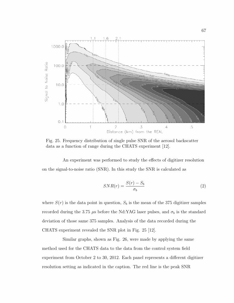
67
Fig. 25. Frequency distribution of single pulse SNR of the aerosol backscatterdata as a function of range during the CHATS experiment [12].
An experiment was performed to study the effects of digitizer resolution
on the signal-to-noise ratio (SNR). In this study the SNR is calculated as
SNR(r) =S(r)− Sb
σb(2)
where S(r) is the data point in question, Sb is the mean of the 375 digitizer samples
recorded during the 3.75 µs before the Nd:YAG laser pulses, and σb is the standard
deviation of those same 375 samples. Analysis of the data recorded during the
CHATS experiment revealed the SNR plot in Fig. 25 [12].
Similar graphs, shown as Fig. 26, were made by applying the same
method used for the CHATS data to the data from the control system field
experiment from October 2 to 30, 2012. Each panel represents a different digitizer
resolution setting as indicated in the caption. The red line is the peak SNR

68
(a) Digitizer range of 10 volts. Duration of80 days in the CHATS experiment of 2007.
(b) Digitizer range of 10 volts. Duration of7 days (Oct. 2–9, 2012).
(c) Digitizer range of 4 volts. Duration of3 days (Oct. 9–12, 2012).
(d) Digitizer range of 2 volts. Duration of3 days (Oct. 12–15, 2012).
(e) Digitizer range of 1 volt. Duration of 3days (Oct. 15–18, 2012).
(f) Digitizer range of 0.4 volts. Duration of3 days (Oct. 18–21, 2012).
Fig. 26. (Color required.) Frequency distribution of single pulse SNR of theaerosol backscatter data as a function of range during the flashlamp voltagecontrol field experiment.
distribution for the data from the CHATS experiment for comparison against SNR
from the control system field experiment.

69
The SNR is affected by instrument performance and aerosol properties
which vary with the day to day weather. Instrument performance includes both the
transmit energy as well as the digitizer resolution. During the period of operation
from the control system field experiment from which these data are taken, the
transmit energy was relatively constant, as shown in Fig. 21. Also, aerosol
properties for the operating period were similar from day to day. Although Fig. 26
shows changes in SNR due mainly to adjustments in the digitizer resolution, a
future test will include a low elevation-angle stare without scanning for about ten
minutes for each digitizer resolution setting. This will ensure a more constant
atmosphere and transmit energy to produce SNR results that will manifest the
effect of the digitizer resolution setting as much as possible.
Taking instrument performance and atmospheric condition assumptions
into consideration, a significant improvement in SNR is noted during the control
system field experiment. Fig. 26 suggests that the instrument started out with a
lower SNR in the control system field experiment than in the CHATS experiment.
With adjustments to the digitizer the SNR was improved to above that of the
CHATS experiment. Fig. 27 reveals the improvement in SNR during the control
system field experiment alone. The yellow line indicates the peak SNR distribution
for the default 10 volt range setting on the digitizer. The blue line indicates the
peak SNR distribution for the 0.4 volt range setting.
The maximum resolution setting during the control system field
experiment produced an SNR distribution peak of 200 at a range of 1 km. This is
double the SNR distribution peak at a range of 1 km from the CHATS experiment.
The control system field experiment revealed a greater improvement in SNR from
the lowest resolution setting to the highest. The SNR distribution peak of 200 at a
range of 1 km is one order in magnitude greater than that of the SNR distribution

70
Fig. 27. (Color required.) Comparison of SNR peak distribution of the aerosolbackscatter data as a function of range during the control system fieldexperiment. The yellow line indicates the peak SNR distribution for the default10 volt range setting on the digitizer and the blue line for the 0.4 volt rangesetting. Overall improvement at 1 km range during the experiment was an SNR ofabout 20 to an SNR of about 200.
peak of 20 at a range of 1 km for the lowest resolution setting in the same
experiment. The digitizer setting resolution has a significant impact on the
performance of the system.
A study was performed prior to this work to analyze how SNR is related
to the spatial wind field measurements of the lidar [12]. Fig. 28 shows the
distributions of velocity component differences in lidar measurements and sonic
anemometer measurements as a function of average SNR for the CHATS
experiment. As SNR increases, the distribution in measurement difference narrows.
This shows that the wind measurement benefits from efforts to improve the SNR of
the backscatter data.

71
Fig. 28. Distributions of wind velocity component differences as a function ofaverage SNR in the cross-correlation blocks used to derive the lidar vectors.Contour interval labels are in percent. The bar chart to the right of each contourplot shows the number of data points in each SNR bin interval. The width of thedistribution of velocity component differences tends to decrease as the SNRincreases [12].
Data Normalization
Prior to this research the backscatter waveforms captured by the
digitizer appeared to have a random vertical offset from one pulse to the next. This
produced radial striations visible in scan images. The leading hypothesis theorized
it was the result of transmit energy variation from pulse to pulse. However, when
the voltage produced from the InGaAs detector was observed directly, the vertical
offset was not present. The background signal, calculated from pre-trigger samples
recorded before the pulse of the laser was sensed, maintained a constant level. The
erratic vertical offsets were a result of a previous unsuccessful effort to normalize
the backscatter data.
Therefore, the normalization process was completely redesigned to
normalize the signal by offsetting the average background (pre-trigger) level of each
channel to a constant. This process does not change the amplitude of the

72
waveforms but shifts them to have equal average background levels. The erratic
vertical offsets were minimized and the radial striations were significantly reduced.
Fig. 29 highlights the differences between the unnormalized (Fig. 29a) and the
normalized (Fig. 29b) data. Fig. 30a and Fig. 30b magnify the striations to more
clearly show the differences.
(a) Unnormalized full scan data (b) Normalized full scan data
Fig. 29. (Color required.) Comparison of unnormalized (left) and normalized(right) full scan data. These images are examples of vertical scans that can revealthe atmospheric boundary layer at lower altitudes and clouds aloft.
(a) Magnification of unnormalized data (b) Magnification of normalized data
Fig. 30. (Color required.) Magnified comparison of unnormalized and normalizedfull scan data.

73
Darker red radial stripes shown in Fig. 30a are, at times, more or less
apparent. This case is considered typical. The normalization was applied to each
pulse from one scan to the next and, therefore, these two scans are separated in
time by about 20 seconds.
BSCAN File Header
Atmospheric backscatter signal is detected, digitized, and written to disk
in the BSCAN file format. These files are written in the form of a two-dimensional
array as shown in Fig. 31. Each row represents the result of a single pulse into the
atmosphere. The first 30 words of a row make up the header for each record in a
BSCAN file. A description of the header is given in Table 5. Following the 30-word
header are the two waveforms: the first channel of the digitizer followed by the the
second. There is one channel for each component of polarization in the received
backscatter signal.
Fig. 31. BSCAN file format organization. Rows represent laser pulses. The first30 columns represent the header and the other columns hold the backscatter data.

74
TABLE 5BSCAN Data File 30-Word Header Format
Number Header Word Name Units1 Hour2 Minute3 Second4 GPS Altitude Meters5 Platform Roll Degrees6 Platform Pitch Degrees7 BSU Azimuth from North Degrees8 BSU Elevation Above Horizon Degrees9 Beam Centroid X Location Pixels
10 Beam Centroid Y Location Pixels11 Beam Radius Millimeters12 Month13 Day14 Year15 Laser Pulse Repetition Frequency Hertz16 Transect Number17 REAL Identifier 22018 (not used)19 Latitude Degrees20 Longitude Degrees21 Range of First Data Point Meters22 Range Bin Size23 (not used)24 Number of Header Words25 (not used)26 (not used)27 Channel A Normalization Energy28 Channel B Normalization Energy29 Number of Lidar Profile Data Points30 Scan Number
This table lists the variables stored in each of the 30 words of theBSCAN data file header. The file contains one header per recordand one record per laser pulse.
The 30 words contained in the BSCAN header are available for recording
system data other than backscatter. There were nine words available in the header

75
that were not used at the time of this study. The header was modified to include
beam centroid location on the X and Y axes, the beam radius, and the absolute
attitude of the platform on the pitch (longitudinal) and the roll (transverse) axes.
The centroid location and beam radius are critical indicators of the beam quality
and it was decided that a per pulse record would be very useful for post operation
data analysis. Absolute attitude angles were included for use in future work to
precisely determine the position of the beam as a function of range. This is
discussed in more detail in Chapter V.
One Scan per BSCAN File
Prior to this study the BSCAN files were about 1.5 gigabytes in size and
contained many scans. The large size of these files made network transfer
problematic. Therefore, the BSCAN files were limited to contain only one scan per
file. The size of the files now is directly related to the duration of the scan and
typically ranges from 3 to 8 MB.
One sweep per BSCAN file creates files of manageable sizes that are
easily organized, transferred, and processed in near-real-time. Each BSCAN file
name includes the date and time of the beginning of the sweep. Data directories
are now easily navigated when looking for a specific time interval or scan. The
smaller size of the files also aids in the transfer of data to the server on the main
campus via secure file transfer program (SFTP). Once on the server, the data are
immediately available to web applications and further processing without affecting
the instrument. This facilitates additional near-real-time processing of the data.
System Variable Measurements File
System variable measurements were recorded once per minute prior to
this study. In the new system design these files are recorded once per BSU sweep to
correspond with the BSCAN files. The system variable measurements file naming

76
convention also contains the same date and time as the BSCAN files. This provides
a record with an average measurement of each system variable that corresponds to
each BSCAN file. These files are also transfered to the main campus server via
SFTP and are used in analyzing performance and diagnosing failure symptoms.
Black Box
After a system failure, engineers need to know as much as possible about
the system conditions that lead to the failure. The system variable measurements
are recorded once per scan (normally about once every 15 to 20 seconds). However,
in the case of a system failure that developed quickly, a low-rate record with data
samples a few times a minute may be inadequate for diagnosing the cause.
Therefore, a “black box” was designed that records system variable measurements
for each laser pulse for the last operator-specified number of minutes of operation.
Now that this black box is installed, high-rate data is available for detailed analysis
to determine the reason for the shutdown.
During the October 2012 testing, BSU failures occurred during horizontal
scans in which the BSU motors momentarily lost power and stopped responding. In
the process of debugging the failure, which occurred about once every 24 hours and
usually at the beginning of a horizontal scan, the azimuth and elevation angles of
the BSU were added to the list of black box variables recorded. This provided an
exact record of when and where the BSU lost power and stopped scanning.
Testing and Results
The majority of the control system implementation took place between
March and October of 2012. As soon as a subsection of code was designed and
tested, it was implemented into the instrument. The control system was built in
this way: piece by piece. Each control subsection was tested thoroughly with

77
simulation data by an integration test procedure. The LabVIEW coding
environment provides excellent code reusability features as well as subprogram
isolation that made for efficient testing.
Improvements in data quality and control were made from the beginning
of the study. On July 20th at 10:35 a.m., a system failure resulted in one of the
prisms in the Raman cell being damaged. The fail-safe control subsection that had
been implemented prior to that point recognized the problem and executed a safe
shutdown procedure. The response time was less than 500 ms and damage was
contained to one prism. Repairs were made to the Raman cell and the system was
operational again on the evening of August 16th. Had the control system not been
in place the damage might have extended to the other prisms or windows of the
Raman cell before personnel noticed. If one of the two windows had been damaged,
a leak of compressed gas from the Raman cell may have resulted.
Although the July 20th case was the most extreme case of system failure
caught by the control system, there have been a number of smaller incidences in
which changing variables were identified and adjustments were made. These
smaller incidences include changes in temperature due to changes in outdoor
weather conditions, changes in pressure due to a very slow, known leak in a Raman
cell, changes in the utility power due to an area-wide power outage, and changes in
beam quality due to the age of the flashlamps.
A whole system test was conducted to exercise the entire design. The
experiment began on October 2, 2012. The purpose of this experiment was to
operate the lidar unattended for the life of a set of flashlamps. The anticipated
flashlamp life was set at 20 million pulses. If the instrument operated continuously,
the experiment would last 23.7 days. The system took approximately 40 minutes to
set up and start. Another hour was spent monitoring the system to ensure proper

78
variable thresholds and operating conditions. After this start-up procedure,
personnel did not assist or monitor the instrument for the duration of the
experiment (25 days of operation excluding a three day interruption from a rain
storm).

CHAPTER V
SUMMARY
This study demonstrated that the high pulse-energy atmospheric lidar at
CSUC, with the control system presented in this work, can operate in a fail-safe
manner with automatic flashlamp voltage adjustment. Potential research and
commercial lidar applications, in which long-term spatial wind field and
atmospheric boundary layer height measurements are required, motivated this
study.
During design and testing to explore which of the proposed control
solutions were viable, some proved to be effective while others were discarded or
modified on an on-going basis. The resulting control system enabled the instrument
to be improved in the following ways: (1) control of the flashlamp voltage to
increase stability of transmit energy during operation, (2) a fail-safe feature to
detect emerging problems and prevent them from escalating and damaging other
system components, (3) a communication feature that notifies personnel of
significant changes in the status of operation, and (4) several data quality
improvements that produce more uniform, organized, and optimized backscatter
energy data. With this newly redesigned control system, the original REAL is now
better-suited for long-term and unattended spatial wind field and atmospheric
boundary layer height measurements.
After implementation and testing of the new control system, an
experiment was performed that demonstrated unattended and continuous operation
79

80
for the lifetime of one set of flashlamps (about 23 days). Performance was
compared to data from an experiment in 2007 during which the instrument was
operated for 80 days (3 sets of flashlamps) without the fail-safe or flashlamp voltage
adjustment features. The comparison revealed improvements in the trend and
stability of transmit energy. A redesign of the data normalization process, digitizer
resolution settings, and data file organization improved data quality.
The control system presented in this work facilitates improved spatial
wind field and atmospheric boundary layer height measurements over long periods
of continuous and unattended operation. This new capability of the lidar opens
opportunities for deployment in meteorological research and commercial
applications. These opportunities include: wind resource assessment that requires
long-term monitoring to determine wind energy potential in challenging-to-reach
locations and altitudes, wind turbine efficiency improvements that use incoming
wind vector measurements to optimize the pitch of rotor blades and yaw of the
hub, air quality forecasting improvements with measurements of boundary layer
height, tracking the dispersion of potentially hazardous emissions from industrial
sites, and increased airport safety and efficiency with observations of wake vortices
and wind shears that may be hazardous to aircraft.
The results of this study have significantly improved the performance
stability and ease of operation of the original REAL. The instrument is now better
equipped to collect measurements during the experiment that will be conducted
between June and November 2013 under NSF AGS 1228464.

REFERENCES

REFERENCES
[1] W. Musial and B. Ram, Large-Scale Offshore Wind Power in the United States.
The National Renewable Energy Laboratory, 2010. [Online]. Available:
http://www.nrel.gov/wind/pdfs/40745.pdf
[2] M. C. Brower, Offshore Resource Assessment. John Wiley & Sons, Inc., 2012,
pp. 195–219. [Online]. Available:
http://dx.doi.org/10.1002/9781118249864.ch14
[3] B. Jimenez, F. Durante, B. Lange, T. Kreutzer, and J. Tambke, “Offshore
wind resource assessment with WAsP and MM5: comparative study for the
German Bight,” Wind Energy, Vol. 10, No. 2, pp. 121–134, 2007. [Online].
Available: http://dx.doi.org/10.1002/we.212
[4] Energy Efficiency and Renewable Energy, “20% wind energy by 2030,” U.S.
Department of Energy, 2008. [Online]. Available:
http://www.20percentwind.org/20percent wind energy report revOct08.pdf
[5] N. Wang, K. Johnson, and A. Wright, “Lidar-based FX-RLS feedforward
control for wind turbine load mitigation,” in American Control Conference
(ACC), 2011, Jul. 2011, pp. 1910–1915.
[6] Committee on Urban Meteorology: Scoping the Problem, Defining the Needs;
Board on Atmospheric Sciences and Climate; Division on Earth and Life
Sciences; National Research Council, “Urban meteorology: Forecasting,
82

83
monitoring, and meeting users’ needs,” 2012. [Online]. Available:
http://www.nap.edu/openbook.php?record id=13328
[7] Committee on Developing Mesoscale Meteorological Observational Capabilities
to Meet Multiple Needs, National Research Council, “Observing weather and
climate from the ground up: A nationwide network of networks,” 2009.
[Online]. Available: http://www.nap.edu/openbook.php?record id=12540
[8] Committee on the Atmospheric Dispersion of Hazardous Material Releases,
National Research Council, “Tracking and predicting the atmospheric
dispersion of hazardous material releases: Implications for homeland security,”
2003. [Online]. Available:
http://www.nap.edu/openbook.php?record id=10716
[9] Committee on Low-Altitude Wind Shear and Its Hazard to Aviation,
Aeronautics and Space Engineering Board, Atmospheric Sciences and Climate
Board, National Research Council, “Low-altitude wind shear and its hazard to
aviation,” 1983. [Online]. Available:
http://www.nap.edu/openbook.php?record id=558
[10] National Academy of Sciences, Wake Turbulence: An Obstacle to Increased
Air Traffic Capacity. National Academies Press, 2008.
[11] M. Margulis and T. Baynard, “Clear shear,” Meteorological Technology
International, pp. 74–77, Aug. 2012.
[12] S. D. Mayor, J. P. Lowe, and C. F. Mauzey, “Two-component horizontal
aerosol motion vectors in the atmospheric surface layer from a cross-correlation
algorithm applied to elastic backscatter lidar data,” J. Atmos. Ocean.
Technol., Vol. 29, pp. 1585–1602, 2012.

84
[13] K. J. Davis, N. Gamage, C. R. Hagelberg, C. Kiemle, D. H. Lenschow, and
P. P. Sullivan, “An objective method for deriving atmospheric structure from
airborne lidar observations,” J. Atmos. Ocean. Technol., Vol. 17, pp.
1455–1468, 2000.
[14] S. D. Mayor, “Raman-shifted Eye-safe Aerosol Lidar (REAL) observations at
the Canopy Horizontal Array Turbulence Study (CHATS),” in 18th
Symposium on Boundary Layers and Turbulence. AMS, 2008.
[15] ——, “Horizontal motion vectors from cross-correlation: First application to
eye-safe aerosol lidar data from CHATS,” in 25th International Laser Radar
Conference, 2010.
[16] E. G. Patton et al., “The Canopy Horizontal Array Turbulence Study
(CHATS),” Bull. Amer. Meteor. Soc., Vol. 92, pp. 593–611, 2011.
[17] E. Jaska, “Optimal power-aperture balance,” in Proc. of the IEEE Radar
Conference, 2003, May 2003, pp. 203–209.
[18] W. Eberhardt, G. Pressler, and K. Guenther, “Cathode erosion and electrode
loss power in pulsed discharges at high pressure,” Beitrage aus der
Plasmaphysik, Vol. 14, No. 2, pp. 51–54, 1974. [Online]. Available:
http://dx.doi.org/10.1002/ctpp.19740140204
[19] Technical Features, Sigma Space Corporation, 2011. [Online]. Available:
http://dx.doi.org/10.1002/9781118249864.ch14
[20] J. D. Spinhirne, S. Chudamani, J. F. Cavanaugh, and J. L. Bufton, “Aerosol
and cloud backscatter at 1.06, 1.54, and 0.53 µm by airborne

85
hard-target-calibrated Nd : YAG/ methane Raman lidar,” Appl. Optics,
Vol. 36, pp. 3475–3490, 1997.
[21] C. J. Grund and E. W. Eloranta, “University of Wisconsin high spectral
resolution lidar,” Opt. Eng., Vol. 30, pp. 6–12, 1991.
[22] E. W. Eloranta and D. K. Forrest, “Volume-imaging lidar observations of the
convective structure surrounding the flight path of a flux-measuring aircraft,”
J. Geophys. Res, Vol. 97, pp. 18 383–18 393, 1992.
[23] C. Weitkamp, Lidar: Range-Resolved Optical Remote Sensing of the
Atmosphere, Ser. Springer Series in Optical Sciences. Springer, 2005. [Online].
Available: http://books.google.com/books?id=8AT2smoj4MkC
[24] T. H. Maiman, “Stimulated optical radiation in ruby,” Nature, Vol. 187, pp.
493–494, 1960.
[25] E. D. Hinkley, Laser monitoring of the atmosphere, Ser. Topics in applied
physics. Springer-Verlag, 1976. [Online]. Available:
http://books.google.com/books?id=pNTvAAAAMAAJ
[26] W. Gaughan and B. Butka, “Using an FPGA digital clock manager to
generate sub-nanosecond phase shifts for lidar applications,” in Programmable
Logic Conference (SPL), 2010 VI Southern, Mar. 2010, pp. 163–166.
[27] Y. Lin, J. Hyyppa, and A. Jaakkola, “Mini-UAV-borne lidar for fine-scale
mapping,” Geoscience and Remote Sensing Letters, IEEE, Vol. 8, No. 3, pp.
426–430, May 2011.
[28] C. Niclass, A. Rochas, P.-A. Besse, and E. Charbon, “Design and
characterization of a CMOS 3-D image sensor based on single photon

86
avalanche diodes,” IEEE Journal of Solid-State Circuits, Vol. 40, No. 9, pp.
1847–1854, Sep. 2005.
[29] S. Hernandez-Marin, A. Wallace, and G. Gibson, “Multilayered 3D lidar image
construction using spatial models in a Bayesian framework,” IEEE
Transactions on Pattern Analysis and Machine Intelligence, Vol. 30, No. 6, pp.
1028–1040, Jun. 2008.
[30] I. Razenkov, H. Cha, D. Kim, and J. Lee, “Measurement of air vertical motion
in the atmosphere by aerosol micro pulse lidar,” in The Pacific Rim
Conference on Lasers and Electro-Optics, 1999 (CLEO/Pacific Rim ’99),
Vol. 2, 1999, pp. 139–140.
[31] J. D. Spinhirne, “Micro pulse lidar,” IEEE Trans. Geosci. Remote Sensing,
Vol. 31, pp. 48–55, 1993.
[32] A. Ansmann, “Errors in ground-based water-vapor DIAL measurements due to
Doppler-broadened Rayleigh backscattering,” Appl. Opt., Vol. 24, No. 21, pp.
3476–3480, Nov. 1985. [Online]. Available:
http://ao.osa.org/abstract.cfm?URI=ao-24-21-3476
[33] V. A. Kovalev and W. E. Eichinger, Elastic Lidar: Theory, Practice, and
Analysis Methods. Hoboken, NJ: John Wiley & Sons, Inc., 2005.
[34] C. L. Korb and C. Y. Weng, “A theoretical study of a two-wavelength lidar
technique for the measurement of atmospheric temperature profiles,” J. Appl.
Meteor., Vol. 21, pp. 1346–1355, 1982.

87
[35] P. Rairoux et al., “Remote sensing of the atmosphere using ultrashort laser
pulses,” Applied Physics B, Vol. 71, pp. 573–580, 2000. [Online]. Available:
http://dx.doi.org/10.1007/s003400000375
[36] F. A. Theopold and J. Bosenberg, “Differential absorption lidar measurements
of atmospheric temperature profiles: Theory and experiment,” J. Atmos.
Oceanic Technol., Vol. 10, pp. 165–179, 1993.
[37] S. D. Mayor, S. M. Spuler, B. M. Morley, and E. Loew, “Polarization lidar at
1.54-microns and observations of plumes from aerosol generators,” Opt. Eng.,
Vol. 46, p. DOI: 10.1117/12.781902, 2007.
[38] E. Burrows and K.-Y. Liou, “High resolution laser lidar utilising two-section
distributed feedback semiconductor laser as a coherent source,” Electronics
Letters, Vol. 26, No. 9, pp. 577–579, Apr. 1990.
[39] G. Busch et al., “Acousto-optically tuned isotopic CO2 lasers for long-range
differential absorption lidar,” in Summaries of Papers Presented at the
Conference on Lasers and Electro-Optics (CLEO) ’97, Vol. 11, May 1997, pp.
188–189.
[40] C. Weitkamp, Lidar: Range-Resolved Optical Remote Sensing of the
Atmosphere. New York: Springer, 2005.
[41] A. Ansmann, M. Riebesell, and C. Weitkamp, “Measurement of atmospheric
aerosol extinction profiles with a Raman lidar,” Opt. Lett., Vol. 15, No. 13, pp.
746–748, Jul. 1990. [Online]. Available:
http://ol.osa.org/abstract.cfm?URI=ol-15-13-746

88
[42] D. N. Whiteman, S. H. Melfi, and R. A. Ferrare, “Raman lidar system for the
measurement of water vapor and aerosols in the Earth’s atmosphere,” Appl.
Opt., Vol. 31, No. 16, pp. 3068–3082, Jun. 1992. [Online]. Available:
http://ao.osa.org/abstract.cfm?URI=ao-31-16-3068
[43] N. Parikh and J. Parikh, “Reducing uncertainties in aerosol retrievals from
micro pulse lidar measurements,” in Geoscience and Remote Sensing
Symposium (IGARSS) 2000. IEEE International, Vol. 2, 2000, pp. 840–842.
[44] K. Rothe, U. Brinkmann, and H. Walther, “Applications of tunable dye lasers
to air pollution detection: Measurements of atmospheric NO2 concentrations
by differential absorption,” Applied Physics A: Materials Science & Processing,
Vol. 3, pp. 115–119, 1974, 10.1007/BF00884408. [Online]. Available:
http://dx.doi.org/10.1007/BF00884408
[45] K. Sassen, “Advances in polarization diversity lidar for cloud remote sensing,”
Proc. of the IEEE, Vol. 82, No. 12, pp. 1907–1914, Dec. 1994.
[46] R. Measures, Laser remote sensing: fundamentals and applications, Ser.
Wiley-Interscience publication. Wiley, 1984. [Online]. Available:
http://books.google.com/books?id=8Z8sAQAAMAAJ
[47] C.-Y. She, “Spectral structure of laser light scattering revisited: Bandwidths of
nonresonant scattering lidars,” Appl. Opt., Vol. 40, No. 27, pp. 4875–4884, Sep.
2001. [Online]. Available: http://ao.osa.org/abstract.cfm?URI=ao-40-27-4875
[48] A. T. Young and G. W. Kattawar, “Rayleigh-scattering line profiles,” Appl.
Opt., Vol. 22, No. 23, pp. 3668–3670, Dec. 1983. [Online]. Available:
http://ao.osa.org/abstract.cfm?URI=ao-22-23-3668

89
[49] J. Marshall, T. East, K. Gunn, and W. Hitschfeld, “The effect of particle
shape and composition on microwave attenuation and scattering by
precipitation,” Transactions of the IRE Professional Group on Antennas and
Propagation, Vol. 3, pp. 180–185, Aug. 1952.
[50] B. Murphy and W.-J. Kim, “Intuitive representation of gain schedulers to
facilitate their design and tuning,” in Proc. of the American Control
Conference, 2004, Vol. 2, Jul. 2004, pp. 1115–1120.
[51] F. Blanchini and S. Miani, “Gain scheduling versus robust control of LPV
systems: The output feedback case,” in American Control Conference (ACC),
2010, Jul. 2010, pp. 3871–3876.
[52] V. Alekseyev, S. Babichenko, and I. Sobolev, “Control and signal processing
system of hyperspectral FLS lidar,” in 11th International Biennial Baltic
Electronics Conference (BEC) 2008, Oct. 2008, pp. 349–352.
[53] S. D. Mayor and S. M. Spuler, “Raman-shifted Eye-safe Aerosol Lidar,” Appl.
Optics, Vol. 43, pp. 3915–3924, 2004.
[54] S. D. Mayor, S. M. Spuler, and B. M. Morley, “NCAR’s New Raman-Shifted
Eye-Safe Aerosol LIDAR (REAL),” in 22nd International Laser Radar
Conference (ILRC 2004), Ser. ESA Special Publication, G. Pappalardo and
A. Amodeo, Eds., Vol. 561, Jun. 2004, p. 53.
[55] S. D. Mayor et al., “Elastic backscatter lidar observations of a gust front
passage over Washington DC on 7 May 2004,” in 7th Symp. on the Urban
Environment. AMS, 2007.

90
[56] T. Warner et al., “The Pentagon Shield Field Program: Toward Critical
Infrastructure Protection,” Bull. Amer. Meteor. Soc., Vol. 88, pp. 167–176,
2007.
[57] S. M. Spuler and S. D. Mayor, “Scanning eye-safe elastic backscatter lidar at
1.54 microns,” J. Atmos. Ocean. Technol., Vol. 22, pp. 696–703, 2005.
[58] P. L. Ponsardin, C. S. Kletecka, R. D. Babnick, K. Krubsack, S. D. Mayor,
and S. M. Spuler, “Autonomous eye-safe lidar for continuous monitoring of
atmospheric aerosols,” in 2006 International Symposium on Spectral Sensing
Research (2006-ISSSR), 2006.
[59] S. D. Mayor, P. Benda, C. E. Murata, and R. J. Danzig, “Lidars: A key
component of urban biodefense,” Biosecur. Bioterror., Vol. 6, pp. 45–56, DOI:
10.1089 bsp.2007.0053, 2008.
[60] R. J. Danzig, “Ideas: Lidar as a lifeline in confronting bioterrorism,” Bull.
Amer. Meteor. Soc., Vol. 87, pp. 731–733, 2006.
[61] S. D. Mayor, “Observations of seven density current fronts in Dixon,
California,” Mon. Wea. Rev., Vol. 139, pp. 1338–1351, 2011.
[62] E. R. Jachens and S. D. Mayor, “Lidar observations of fine-scale atmospheric
gravity waves in the nocturnal boundary layer above an orchard canopy,” in
26th International Laser Radar Conference, Jun. 2012.
[63] S. D. Mayor, E. R. Jachens, and T. N. Randall, “Lidar observations of
fine-scale gravity waves in the nocturnal boundary layer above an orchard
canopy,” in 16th International Symposium for the Advancement of
Boundary-Layer Remote Sensing (ISARS), Jun. 2012.

91
[64] T. N. Randall, E. R. Jachens, and S. D. Mayor, “Lidar observations of
fine-scale atmospheric gravity waves in the nocturnal boundary layer above an
orchard canopy,” in American Meteorological Society’s 20th Symposium on
Boundary Layers and Turbulence, Jul. 2012.
[65] S. D. Mayor. (2012) Atmospheric lidar research group. California State
University, Chico. [Online]. Available: http://phys.csuchico.edu/lidar/
[66] American National Standards Institute and Laser Institute of America,
“American national standard for safe use of lasers: ANSI Z136.1-2000,” 2000.
[Online]. Available: http://books.google.com/books?id=IfIwRAAACAAJ
[67] S. M. Spuler and S. D. Mayor, “Raman shifter optimized for lidar at
1.5-micron wavelength,” Appl. Optics, Vol. 46, pp. 2990–2995, 2007.
[68] ——, “Eye-safe aerosol lidar at 1.5 microns: progress towards a scanning lidar
network,” in SPIE Lidar Remote Sensing for Environmental Monitoring VIII,
San Diego, CA, 2007, p. DOI: 10.1117/12.739519.
[69] E. M. Patterson, D. W. Roberts, and G. G. Gimmestad, “Initial measurements
using a 1.54 micron eyesafe raman shifted lidar,” Appl. Optics, Vol. 28, pp.
4978–4981, 1989.
[70] W. Carnuth and T. Trickl, “A powerful eyesafe infrared aerosol lidar:
Application of stimulated raman backscattering of 1.06 micron radiation,”
Rev. Sci. Instrum., Vol. 65, pp. 3324–3331, 1994.
[71] NI PXI/PCI-5122 Specifications, National Instruments, 2004. [Online].
Available: http://www.ni.com/pdf/manuals/323497b.pdf

APPENDIX A

APPENDIX A
FUTURE WORK
During the course of this research, several improvements of the lidar
that would increase both the quality of backscatter data and reliability and ease of
operation were identified. Ten possible improvements are listed and discussed in
this Appendix.
Temperature Stabilization
As shown in Fig. 20, the time-series plot of system temperatures and
vital signs from the gain scheduler control field experiment, the temperature affects
the performance of the instrument. Stability in the temperature of the housing
container is highly correlated to transmit pulse-energy and conversion efficiency. It
is hypothesized that variations in temperature have a significant impact on
instrument performance in the form of thermal lensing of the Nd:YAG rod. The
Nd:YAG rod used in this study is relatively long and manifests thermal lensing as
the rod is heated more on the axis of the beam than on the outer regions. This
temperature variation in the rod causes transverse gradients of the refractive index
of the rod. Temperature variations in the laser head accentuate this effect. The
Nd:YAG beam divergence is directly related to the beam energy density and
conversion efficiency through the Raman cell. Temperature stabilization in the
laser head would reduce changing of the thermal lensing of the Nd:YAG rod.
93

94
The laser head is cooled with a water circulation system and a heat
exchanger that exhausts hot air into the housing container of the lidar. This
system circulates about a liter of water through a reservoir and two radiators. The
radiators cool the water in direct proportion to the air temperature in the housing
container. It is hypothesized that temperature stabilization may be achieved by
increasing the size of the reservoir, and therefore the thermal mass of the water
that cools the laser head. Also, the heat exchangers could be more isolated so the
cooling process would not be so sensitive to slight changes in the air temperature in
the housing container.
Real-Time Operating System
The control system of the lidar at CSUC has the ability to substitute
the 10 Hz laser with a faster rate laser of 20 to 100 Hz. Incorporating a faster rate
laser would require a real-time operating system (RTOS) which would take months
to properly configure, test, and implement. Chapter IV discussed this limitation as
it pertains to processing constraints and speeds of the control loop. The most
viable solution found for RTOS was the NI Real-Time Module. This is a software
package that allows a PC to run an RTOS that can be supervised by another PC
running Windows 7. The RTOS maximizes the capabilities of the PC to execute a
single operation, which in this case is the operation that controls the lidar.
Adding Beam Energies and Conversion Efficiency to BSCAN File Header
This study added beam location, beam radius, and absolute attitude of
the housing container platform to the BSCAN file header. At the start of the
experiment it was decided that it would also be beneficial to have the Nd:YAG
beam and transmit beam energies and the conversion efficiency included in the

95
header. With these additions, each pulse of the lidar has on record the
corresponding beam location, radius, energies, and conversion efficiency, along with
the absolute attitude of the platform. As mentioned earlier in this study, these
variables are the “vital signs” of performance.
Smaller Flashlamp Voltage Increments
The 11 flashlamp voltage settings limit the quality of the control
available for design. This limitation is the result of the manufacturer’s design that
offers a simple operator interface. The laser was meant to be adjusted manually,
not automatically, which led to the design of crude adjustment increments of 10
volts. However, if the flashlamp voltage could be controlled in increments of 1 volt
or even 0.1 volts, the quality of control available would be increased significantly.
Modifying circuitry in the Nd:YAG laser power and cooling unit could accomplish.
This project should be done in consultation or partnership with the laser
manufacturer.
Experiments might also include the feasibility of transmit energy control
using the Q-switch delay with or in place of the flashlamp voltage. The Q-switch
delay offers a finer incrementation. For example, a range from 225 to 275 µs could
be used in increments of 1 µs. The Q-switch delay does not adjust the radiation
emitted from the flashlamps, as the flashlamp voltage does, but adjusts the
pulse-energy output from the laser head given the radiation from the flashlamps.
Automated Digitizer Resolution
The control system designed in this study allows personnel to change
the digitizer resolution (range and offset) without interrupting the continuous
operation of the lidar. As the BSU returns from finishing a scan to the start angles

96
of the next scan, the digitizer is able to recalibrate with the updated resolution
settings. A future project will automate this feature to recognize atmospheric
conditions and adjust the resolution for optimal data capture. As shown in Fig. 24,
the InGaAs detector waveform read by the digitizer is no more than a volt in
amplitude. The two settings available for digitizer resolution adjustment are a 1.0
volt range and a 0.4 volt range. InGaAs sensor clipping at long ranges may be used
to detect which amplitude would best suit atmospheric conditions. The
recalibration would then take place automatically.
Beam Quality Control
In the design presented in this study, the control feature is given the
number of pulses on the current set of flashlamps as an input and the flashlamp
control voltage is output to the system. Other inputs were explored as possible
substitutes for the pulse count. Nd:YAG and transmit beam energies were
investigated but proved to have limited dependability. Conversion efficiency (1.5
µm energy exiting the Raman cell divided by 1 µm energy entering) was found to
be a more stable and reliable variable that provided a better reflection of the
flashlamp control voltage on the beam. This variable could be investigated as a
possible input to the gain scheduler flashlamp voltage control. This project would
likely be done in conjunction with the temperature stabilization project and/or the
smaller flashlamp voltage increments project.
Precision BSU Control
Part of this research included writing the absolute attitude of the
housing container platform in the 30 word header of the BSCAN file entries.
Currently, this enables data analysts to precisely calculate the beam altitude at

97
long ranges in post-processing. A similar application could use these measurements
to precisely direct the BSU to compensate for platform pitch and roll. The absolute
attitude sensors are accurate up to 10−6 of a degree and the encoders on the BSU
are accurate up to 10−4 of a degree. This will provide much more accurate beam
placement especially at long ranges. Such capability should be of value in, for
example, offshore wind assessments where precise beam pointing is necessary to
maintain constant altitude. At a 5 kilometer range, a 1 mm roll in the housing
container would displace the beam about 2 meters. An illustration of this effect in
shown in Fig. A.1.
Fig. A.1. An illustration of the effect pitch and roll movements have on the beamat long range. A one millimeter roll in the housing of the container results in atwo meter beam displacement at five kilometers range.
Fig. A.2 displays three days of data from the tiltmeters. A daily cycle is
noted as the heating of the day and cooling of the night cause the instrument

98
housing to expand and contract. The left vertical axis indicates the angle of pitch
and roll while the right is the corresponding vertical displacement of the beam at a
range of 5 km.
Fig. A.2. A three day time series of tiltmeter measurements for pitch and roll ofthe instrument housing at the CSUC field site.
The three days plotted in Fig. A.2 were similar in temperature variation
and resulted in a beam displacement of less than one meter at five kilometers
range. As seasons change temperature variation will increase and, therefore, beam
displacement will occur. The pitch and roll of the container is also sensitive to wind
and movement of personnel on the platform. During the CHATS experiment of
2007 some roll in the container, due to the semi-truck trailer slowly sinking into the
soil, was noticed. Because the system was incapable of sensing its attitude and

99
automatically compensating for the roll, better wind measurement comparisons
with the in situ sonic anemometer could not be made.
GSM Modem Communication
The network connection is used to send email and text notifications.
This is sufficient as long as the network does not fail, in which case notifications
will not reach personnel. A GSM (wireless) modem incorporated into the system
would avoid this problem. If the network failed, the GSM modem would send a
message through the wireless network using the nearest cellphone tower. Wireless
communication is not part of the present design because of implementation cost
and low rate of failure. If the network fails, the control still performs its tasks but
personnel will not become aware until they check on the instrument. Another
feature that could be included to notify personnel of instrument status is a regular
check-in message. At a specific operator-defined interval, the control system would
send a message to personnel indicating that everything is in order. Thus, if a
message is not received at the end of the defined interval, personnel would know
about a problem with the network. I similar solution would include a program on
the campus server to verify the connection to the lidar site periodically and notify
personnel via SMTP if there is a connection failure.
Interfacing to Security System
It could be beneficial for the system to recognize when the lidar security
system has been triggered. The lidar control system could use an analog to digital
converter to read an alarm output, such as a siren, and perform a safe shutdown
procedure. If the system were in operation and a security alarm were tripped, the
control system would perform a safe shutdown procedure.

100
Scan Interval Timing
There is a need to time the scans to occur at a operator-specified time
interval. This feature could be used to stipulate equal amounts of time between
scans (necessary for time-series analysis of wind data) or coordinate the scans with
other equipment in the field. The scan interval would be required to be longer than
the length of the scan. Once the scan is complete the BSU could return to the
starting azimuth and elevation angles and wait for the start of the next interval.
This has proved difficult to implement due to the asynchronous nature of the BSU
motor control commands within the control loop.

APPENDIX B

APPENDIX B
AN OVERVIEW OF THE LABVIEW CODE FOR THE REAL
This appendix contains an overview of the LabVIEW program used to
operate the REAL. Mr. Bruce Morley from NCAR wrote the original code.
Throughout the course of this study the code has been altered to accommodate the
newly developed features. This guide does not discuss all changes that have
occurred but only the final program implemented as a result this study. This
appendix assumes the reader has a basic knowledge of LabVIEW or signal flow.
Due to the graphical nature of LabVIEW, code is somewhat self-explanatory.
Unfortunately, LabVIEW is not easily commented. Just a few comments can easily
clutter a program. This overview is designed to explain some of the code blocks in
the program and how to use them. This is not intended to be an extensive or
detailed instruction guide for programming.
Overview
The REAL LabVIEW program is meant to be read on a rotated, wide
screen monitor to facilitate navigation. This program implements a state machine
with 15 states. The main loop includes 5 of the 15 states. The main structure of
the code is a main case structure enclosed in a while loop structure. Each case in
the case structure is a state in the state machine. The while loop structure is used
to keep the program running and pass information from one state to the next using
102

103
shift registers. Shift registers are located at the top of each side of the while loop
structure and look like big ports with carrots on them.
The values outside the while loop on the left are initialization variables.
The format has to match the format expected in every state by the respective
variables. The actual values are not that important since they will be set in the
initialization states. The initialization of the DataRay WinCamD is visible at the
bottom of the state. Fig. B.1 shows the front panel of the LabVIEW program used
to operate the REAL as it would appear on the computer screen. Fig. B.2 shows
the code in the first state as it would appear on the computer screen. Table B.1
enumerates the state machine states with states included in the main loop marked
with a ?. Fig. B.3 shows the state diagram and Fig. B.4 describes the subroutines
of each state.

104
Fig
.B
.1.
Scr
een
captu
reof
the
fron
tpan
elof
the
Lab
VIE
Wpro
gram
use
dto
oper
ate
the
RE
AL
.
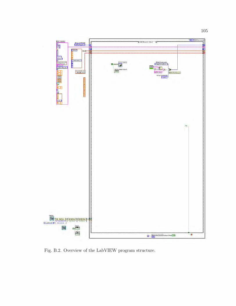
105
Fig. B.2. Overview of the LabVIEW program structure.

106
TABLE B.1State Machine States
Number State Name1 NI PCI Present2 Open Comm Ports3 Initialize NI Card4 Allocate Display Memory5 Start Laser6 Start BSU7 ?Start NI Card8 ?Wait For NI Trigger9 ?Long
10 ?Short11 ?New Scan12 Precip Sleep13 Stop Laser14 Close Comm Ports15 Abort
States included in the main loop are in-dicated with a ?.

107
Fig. B.3. State diagram used to operate the REAL as implemented by theprogram.

108
Fig
.B
.4.
Sta
tes
wit
hsu
bro
uti
ne
des
crip
tion
s.

109
Initialization
There are 6 initialization states. These states setup the variable formats
and operator settings, and calibrate hardware before the system enters the main
loop. Initialization states are:
1. NI PCI Present2. Open Comm Ports3. Initialize NI Card4. Allocate Display Memory5. Start Laser6. Start BSU
NI PCI Present
The NI PCI Present state verifies that the digitizer is present and
operable. If it is not, the system enters the shutdown procedure. In this state the
safety shutter is closed. There is no reason for the safety shutter to be open yet.
Open Comm Ports
This state opens the communication and broadcast ports that will be
used during operation. The code blocks that read “AZ” and “EL” are the azimuth
and elevation angle controls for the BSU motors. Communication ports for the seed
laser, Surelite, and Molectron ports are also opened. The variable “Profiles
Recorded” is initialized to zero and the two broadcast ports, “PPI” and “RHI”, are
opened.
Initialize NI Card
This is the main initialization state. This state was previously divided
into four states. It was decided to combine the four states into one so that only one
pop-up start menu would appear each time the system initialized. The main
subroutine, “Initialize Master.vi,” is half-way down on the left side. Once this .vi is
complete the initialization values are distributed to the appropriate variables.

110
The NI PCI-5122 setup is at the top of the event structure inside
Initialize Master.vi as shown in Fig. B.5.
Fig. B.5. NI PCI-5122 initialization code.
This code initializes and configures the digitizer. The vertical
configuration determines which voltage range the digitizer will read. The options
from the manufacturer’s manual are shown in Table 4 [71]. This code allows the
operator to chose which calibration settings will be used at the beginning of
operation but settings can also be changed once the system is in operation.
Other than the vertical range and offset, the NI PCI-5122 calibration
settings need not be changed. A little farther down are the code blocks for the seed
laser initialization, the Surelite initialization, and then the flashlamp LUT
initialization which is shown in Fig. B.6. The file titled Flashlamp\_LUT.vi
initializes the look-up table (LUT) that the gain scheduler control will use to
determine the flashlamp voltage output. Because the flashlamp voltage is such an
important part of the system, this initialization process minimizes computation
during operation. There are two LUT options: one for a 20 million flashlamp pulse

111
lifetime expectancy and another for a 30 million flashlamp pulse lifetime
expectancy.
Fig. B.6. Flashlamp LUT Setup
The next step in the procedure is the project directory and file setup,
followed by the BSU setup. The routine written for setting the new pulse count
after installing new flashlamps is the event structure that follows next in the state.
Allocate Display Memory
This state first directs the BSU to the starting angles of the first scan.
Then the history length is set on the intensity chart for readability during
operation. The sequential structure starts the flashlamps and lets them warm-up if
necessary. The Molectron energy meters are also initialized.
Start Laser
Once the flashlamps have warmed, the laser is started. The system
variable measurements file (.hk for house-keeping) and black box file (.bb) are also
created and initialized.

112
Start BSU
With the laser pulsing and the BSU pointed in the initial direction, the
scan sequence of the BSU is started without delay.
Main Loop
At this point the program has completed the initialization states and
has entered the main loop of the state machine. The states included in the main
loop are:
1. Start NI Card2. Wait For NI Trigger3. Long4. Short5. New Scan
Start NI Card
The first state in the main loop includes a while loop structure, as
shown in Fig. B.7, at the top on the left side.
Fig. B.7. Code block produces a TRUE value when the system is not collectingdata.
This while loop produces a TRUE signal when the BSU reaches the end
of a scan and starts the return motion, or “fly-back.” This boolean variable is used
throughout the program to execute processes that will be done during the time the
system is not collecting data or as soon as a scan is completed. During the time the

113
BSU is in fly-back, processes are executed that would not be possible during the
scan due to timing restrictions. For example, the vertical configuration of the
digitizer is adjusted. This may take long enough that, if done during a scan, the
delay may result in the loss of backscatter data. Also, if the configuration is
changed during the scan, then part of the scan will have inconsistent resolution
with the other part of the scan.
The most important part of this state is the sub .vi called “niScope
Initiate Acquisition.vi.” If this is not executed, then the trigger from the Nd:YAG
laser will never be seen by the digitizer and the program will be stuck in the Wait
For NI Trigger state until manually aborted. The little bit on the bottom is to close
the receiver box safety shutter if the elevation angle on the BSU ever drops below
zero degrees. This is an attempt to avoid hard target reflections.
Wait For NI Trigger
This is the state that waits for the trigger to be seen by the digitizer so
that the digitizer buffer can be read. The while loop inside the sequential structure,
as seen in Fig. B.8, is how the program waits for the trigger. There is a time out
feature so that if the trigger does not arrive within the allotted time, the problem is
recognized and the system is stopped. As soon as the trigger from the digitizer is
seen, the azimuth and elevation angles of the BSU are recorded to best represent
the beam path in the atmosphere. This is also an appropriate place to manually
measure the timing of the process.

114
Fig. B.8. Wait For NI Trigger code
The next small section of code, shown in Fig. B.9, is the control voltage
for the InGaAs detectors. This code reads the voltage from a temperature sensing
diode and averages the reading over a period of time. The control voltage is
adjusted on the detectors every second. The voltage does not change much, but it
is important because the detectors are very sensitive to temperature.
Fig. B.9. Molectron Temperature Adjustment code
The last bit of code in this state, shown in Fig. B.10, is to set the
priority that LabVIEW has in the operating system. Normally, this would be done
in the Windows Task Manager in the Processes tab by right clicking the Process in
need of a priority change. This piece of code, if enabled, will set the priority while
the system is operating. This code is currently disabled because it needs the
Kernel32.dll to function and the system does not require this feature with the 10
Hz laser. The file Kernel32.dll is in C:/Windows/System32, but the system
doesn’t automatically see it on start up. Also, little improvement was noticed in
processing time when the priority is adjusted.

115
Fig. B.10. System Priority Level Setting
Long
This is the heart of the loop where the majority of computation takes
place. It is called long because it is temporally the longest state. Several sections of
code require significant time to execute and were combined into one state to enable
as much parallel computation as possible. Starting at the top and working down,
the code that reads the digitizer buffer is visible.
The block of code shown in Fig. B.11 calculates the signal-to-noise ratio
of the captured backscatter data. Disabling this code reduces overall processing
time. The SNR is plotted on the same type of chart as the intensity chart. The
purpose of this is to compare the SNR from different scans when changing the
vertical configuration of the digitizer.
Fig. B.11. SNR code
The next bit of code, shown in Fig. B.12, is used to visually verify
digitizer voltage range and offset on the front panel. Adjustments can be made
during operation that are implemented in the Start NI Card state.

116
Fig. B.12. ADC Voltage offset
The next piece of code, shown in Fig. B.13, reads the digitizer buffer.
At this point the trigger indicates that the digitizer’s buffer contains data that is
ready to be read into the program. A .vi is used to read the data from the buffer
into a 2-D array that is split into the two channels, one for each detector. The next
bit of code scales, inverts, and normalizes the data to best represent the backscatter
signal received. Normalization takes the background (pretrigger) level of both
channels, aligns them, and offsets them to the bottom of the data spectrum. This
is often referred to as the raw data. Only offset gain manipulation is performed.
Fig. B.13. Read NI Card
Now the system checks to see if it should be “collecting data.” The
code, shown in Fig. B.14, produces a TRUE for the “collecting data” variable if a
scan is in progress and not in fly-back. This is done by stating, “If current angle
sample is greater than or equal to the previous angle sample, then the system is
collecting data, otherwise, the system is not collecting data.” If the current angle
sample is less than or equal to the previous sample, then the BSU is in fly-back. If
the current angle sample is the same, then the scan is in “stare” mode. If the scan

117
mode is horizontal then the azimuth angle will be the angle of interest, and if it is
vertical the elevation angle will be the angle of interest. If it is a stare then
collecting data is always true.
Fig. B.14. Check BSU movement
The Molectron instrument reads the energies of the Nd:YAG laser beam
and the transmit beam. The two constants, 3.41 and 3.04, are scale factors for the
transmit and Nd:YAG beams, respectively. With these two energy measurement
values, conversion efficiency is calculated. The disabled section of code is used for
the flashlamp voltage experiment mentioned in the body of the thesis. The system
was operated for five minutes on each of the 11 flashlamp voltage levels (1.47, 1.48,
..., 1.56, 1.57 kV). The corresponding energies and conversion efficiencies were
plotted in Fig. 14. The code that reads the Molectron measurements is shown in
Fig. B.15.
Fig. B.15. Molectron Readings

118
The next block of code, shown in Fig. B.16, writes the .hk and .bb files.
The variables that will be recorded are seen on the left as they are “bundled.”
There are two different .hk files because there are two directories. Two .vi’s write
the two files because using one .vi to write both files is unnecessarily slow. The file
Housekeeper\_2012.vi sums the values of each variable during the scan and, right
before writing the value to the file, the total sum is divided by the number of pulses
in the scan to produce an average value of that variable for the scan.
Writing to the .bb files reuses much of the same code as writing to the
.hk files. The difference is that the .bb file is written to after each pulse of the laser
and, once the file reaches a certain number of pulses (ten minutes worth), it writes
in the new values while erasing the oldest values. This records detailed information
about the last 10 minutes of operation. The operator may change the amount of
time recorded inside the file “black box.vi.”
Fig. B.16. House-keeping and black box .vi’s.
The next block of code, shown in Fig. B.17, displays the data on the
front panel of the program. The process is to: normalize to the pretrigger, range
correct ( 1R2 ), and, since displaying data requires significant processing, determine
whether or not to enable the display.

119
Fig. B.17. Data Display Code
The next block of code, shown in Fig. B.18, is the main control .vi’s
that were implemented during this research. Here the system decides to continue
operating if everything is in order. The variables come in from the left. The .vi’s in
the middle are the control blocks. Then all the boolean shutdown signals are OR’d
together. A “Shutdown Cause” indicator appears on the front panel when there is
a shutdown, which facilitates quick identification of failure causes. For every
variable there are contact personnel thresholds and shutdown thresholds. The
notification emails are a custom part of individual .vi’s. This facilitates specificity
in the messages sent to personnel. The only control that happens outside this state
is the utility power control. It uses FTP to read the utility power on the UPSs, so
this process is slow. Fortunately, the UPSs provide power to the system for a half
hour following a power outage which provides plenty of time for the failure to be
detected before the system is affected. This code is located in the New Scan state
and executed when not collecting data.

120
Fig. B.18. Control Block Code
The piece of code at the very bottom, shown in Fig. B.19, is for the
DataRay. Because the DataRay code comes from special .dll’s from the
manufacturer, it cannot be placed in a sub .vi.
Fig. B.19. DataRay Code expanded
The absolute attitude control .vi at the bottom is in a sequential
structure, because it executes only after the file HK\_drive.vi has finished using
the NI SCC-2345. Two .vi’s cannot try to use the device at the same time.

121
Short
After the Long state, next is the Short state. Two processes take place
in this state: write the BSCAN file and broadcast backscatter data. The top part,
shown in Fig. B.20, is the BSCAN file write. Most of what is visible is the
organization of the header. The header format is described in Table 5. Each
BSCAN header word is a 4 byte floating point number. The zeros represent
intentional blank slots in the header. Toward the bottom of the state is the
broadcast code shown in Fig. B.21.
Fig. B.20. Write BSCAN file

122
Fig. B.21. Broadcast data
New Scan
Following the Short state is the New Scan state. After each scan, new
.BSCAN and .hk files are made. The while loop determines that the scan is
completed before a new scan and file are initialized and loaded. This is also the
appropriate time to SFTP the files to the server (before closing the current files).
The current files are closed and new files are created with appropriate names. The
process is the same for both the .BSCAN and the .hk files. The little case structure
that closes and deletes the file just created is used when the stop command has
been recognized. This is to prevent creating empty files in the directory when the
operation is stopped. The code towards the bottom loads the appropriate scan
from the scan sequence queue. The corresponding scan commands are sent to the
BSU motors.
Precipitation Sleep
This state is not considered a state of the main loop. The little while
loop in step 5 is where the system sits and waits for the rain to stop. If the rain
doesn’t stop after an operator-specified number of minutes, a time out feature will
shut down the system. There are two stop buttons to manually abort the sleep

123
mode and continue operating or shut down. The “Precip Continue” button on the
front panel will override the precipitation sleep and continue collecting data even
though there is precipitation. The second button is the “STOP” button. This is
will end the precipitation sleep and stop the system. If the rain does stop in the
allotted time, the while loop is exited, the lower code is executed, and the main
loop is resumed. During the Precipitation Sleep state the flashlamps pulse, but no
laser radiation is emitted from the laser head.
Shutdown
Stop Laser
1. Stop Laser2. Close Comm Ports3. Abort
Stop Laser
This state will stop the flashlamps, stow the BSU into a protective
posture, stop the seed laser, and wait eight seconds. The eight-second wait is to
ensure that the BSU has time to correctly stow before closing the communication
ports to the BSU motors.
Close Comm Ports
This state appropriately closes files and communication ports to the
Nd:YAG laser, the Molectron energy meters, and the broadcast ports.
Abort
This state exits the most outer while loop in the program, ending code
execution. This is the final state of the state machine.