Embed Size (px)
Citation preview
C H A P T E R
CONTROL STRATEGIES FORAUTONOMOUS VEHICLES
Chinmay Samak Tanmay Samak Sivanathan Kandhasamy
Autonomous Systems LaboratoryDepartment of Mechatronics EngineeringSRM Institute of Science and Technology
{cv4703, tv4813, sivanatk}@srmist.edu.in
CONTENTS
1.1 Introduction . . . . . . . . . . . . . . . . . . . . . . . . . . . . . . . . . . . . . . . . . . . . . . . . . . . . . . . . . . . . . . 11.1.1 The Autonomous Driving Technology . . . . . . . . . . . . . . . . . . . . . . . . . . . 11.1.2 Significance of Control System . . . . . . . . . . . . . . . . . . . . . . . . . . . . . . . . . . . 21.1.3 Control System Architecture for Autonomous Vehicles . . . . . . . . . 3
1.2 Mathematical Modeling . . . . . . . . . . . . . . . . . . . . . . . . . . . . . . . . . . . . . . . . . . . . . . . . . . 31.2.1 Kinematic Model . . . . . . . . . . . . . . . . . . . . . . . . . . . . . . . . . . . . . . . . . . . . . . . . . 51.2.2 Dynamic Model . . . . . . . . . . . . . . . . . . . . . . . . . . . . . . . . . . . . . . . . . . . . . . . . . . 8
1.2.2.1 Longitudinal Vehicle Dynamics . . . . . . . . . . . . . . . . . . . . . 81.2.2.2 Lateral Vehicle Dynamics . . . . . . . . . . . . . . . . . . . . . . . . . . . 101.2.2.3 Consolidated Dynamic Model . . . . . . . . . . . . . . . . . . . . . . . 11
1.3 Control Strategies . . . . . . . . . . . . . . . . . . . . . . . . . . . . . . . . . . . . . . . . . . . . . . . . . . . . . . . . 121.3.1 Control Schemes . . . . . . . . . . . . . . . . . . . . . . . . . . . . . . . . . . . . . . . . . . . . . . . . . 12
1.3.1.1 Coupled Control . . . . . . . . . . . . . . . . . . . . . . . . . . . . . . . . . . . . . 121.3.1.2 De-Coupled Control . . . . . . . . . . . . . . . . . . . . . . . . . . . . . . . . . 13
1.3.2 Traditional Control . . . . . . . . . . . . . . . . . . . . . . . . . . . . . . . . . . . . . . . . . . . . . . 131.3.2.1 Bang-Bang Control . . . . . . . . . . . . . . . . . . . . . . . . . . . . . . . . . . 151.3.2.2 PID Control . . . . . . . . . . . . . . . . . . . . . . . . . . . . . . . . . . . . . . . . . 171.3.2.3 Geometric Control . . . . . . . . . . . . . . . . . . . . . . . . . . . . . . . . . . . 201.3.2.4 Model Predictive Control . . . . . . . . . . . . . . . . . . . . . . . . . . . . 28
1.3.3 Learning Based Control . . . . . . . . . . . . . . . . . . . . . . . . . . . . . . . . . . . . . . . . . . 351.3.3.1 Imitation Learning Based Control . . . . . . . . . . . . . . . . . . 361.3.3.2 Reinforcement Learning Based Control . . . . . . . . . . . . . 41
1.4 Our Research at Autonomous Systems Lab (SRMIST) . . . . . . . . . . . . . . . . . 451.5 Closing Remarks . . . . . . . . . . . . . . . . . . . . . . . . . . . . . . . . . . . . . . . . . . . . . . . . . . . . . . . . . 45
arX
iv:2
011.
0872
9v3
[cs
.RO
] 1
0 Se
p 20
21
Control Strategies for Autonomous Vehicles � 1
THIS CHAPTER shall focus on the self-driving technology from a control per-spective and investigate the control strategies used in autonomous vehicles and
advanced driver-assistance systems (ADAS) from both theoretical and practical view-points.
First, we shall introduce the self-driving technology as a whole, including per-ception, planning and control techniques required for accomplishing the challengingtask of autonomous driving. We shall then dwell upon each of these operations to ex-plain their role in the autonomous system architecture, with a prime focus on controlstrategies.
The core portion of this chapter shall commence with detailed mathematicalmodeling of autonomous vehicles followed by a comprehensive discussion on controlstrategies. The chapter shall cover longitudinal as well as lateral control strategiesfor autonomous vehicles with coupled and de-coupled control schemes. We shall aswell discuss some of the machine learning techniques applied to autonomous vehiclecontrol task.
Finally, there shall be a brief summary of some of the research works that ourteam has carried out at the Autonomous Systems Lab (SRMIST) and the chaptershall conclude with some thoughtful closing remarks.
1.1 INTRODUCTION
Autonomous vehicles, or self-driving cars as they are publicly referred to, have beenthe dream of mankind for decades. This is a rather complex problem statement toaddress and it requires inter-disciplinary expertise, especially considering the safety,comfort and convenience of the passengers along with the variable environmentalfactors and highly stochastic fellow agents such as other vehicles, pedestrians, etc.The complete realization of this technology shall, therefore, mark a significant stepin the field of engineering.
1.1.1 The Autonomous Driving Technology
Autonomous vehicles perceive the environment using a comprehensive sensor suiteand process the raw data from the sensors in order to make informed decisions. Thevehicle then plans the trajectory and executes controlled maneuver in order to trackthe trajectory autonomously. This process is elucidated below.
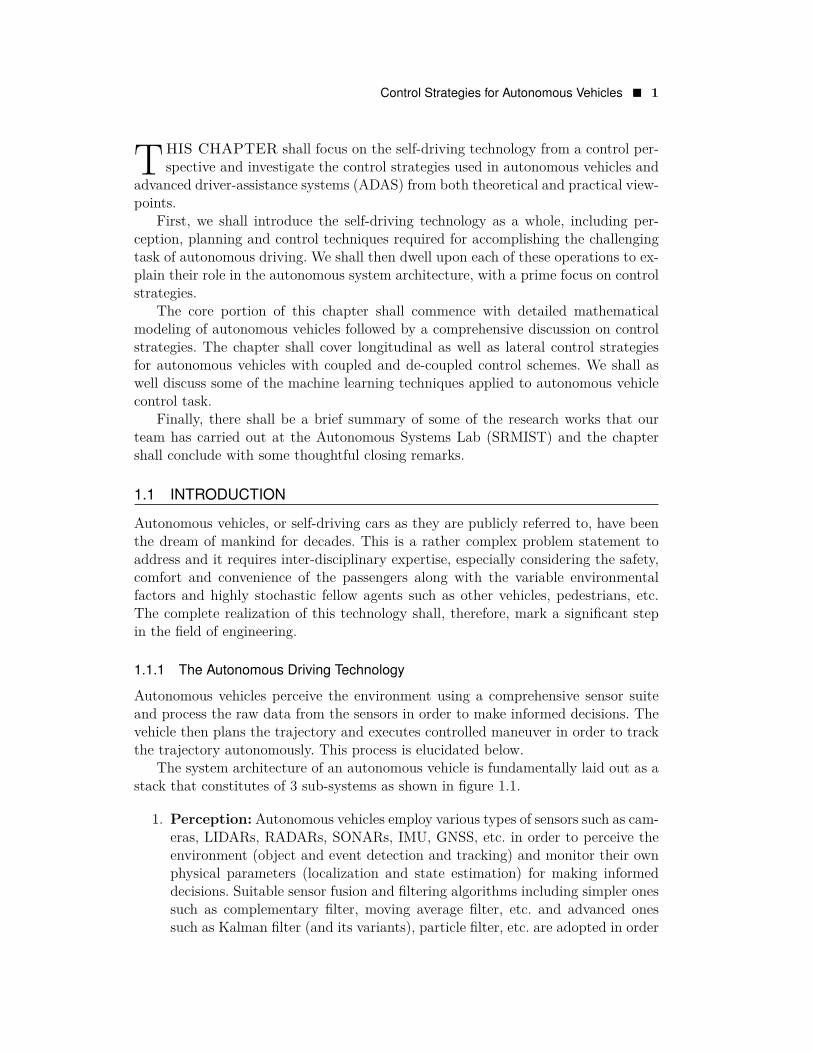
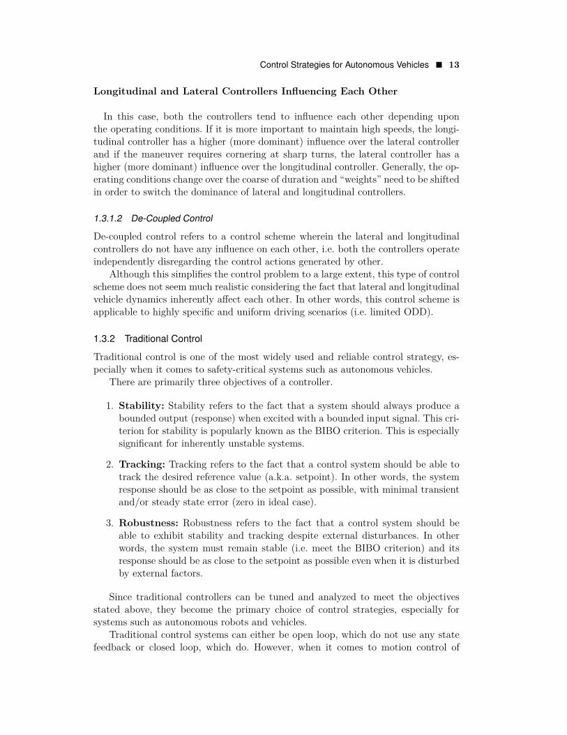
The system architecture of an autonomous vehicle is fundamentally laid out as astack that constitutes of 3 sub-systems as shown in figure 1.1.
1. Perception: Autonomous vehicles employ various types of sensors such as cam-eras, LIDARs, RADARs, SONARs, IMU, GNSS, etc. in order to perceive theenvironment (object and event detection and tracking) and monitor their ownphysical parameters (localization and state estimation) for making informeddecisions. Suitable sensor fusion and filtering algorithms including simpler onessuch as complementary filter, moving average filter, etc. and advanced onessuch as Kalman filter (and its variants), particle filter, etc. are adopted in order
2 � Control Strategies for Autonomous Vehicles
Figure 1.1 System Architecture of an Autonomous Vehicle
to reduce measurement uncertainty due to noisy sensor data. In a nutshell, thissub-system is responsible for providing both intrinsic and extrinsic knowledgeto the ego vehicle using various sensing modalities.
2. Planning: Using the data obtained from the perception sub-system, the egovehicle performs behavior planning wherein the most optimal behavior to beadopted by the ego vehicle needs to be decided by predicting states of the egovehicle as well as other dynamic objects in the environment into the future bycertain prediction horizon. Based on the planned behavior, the motion planningmodule generates an optimal trajectory, considering the global plan, passengersafety, comfort as well as hard and soft motion constraints. This entire process istermed as motion planning. Note that there is a subtle difference between pathplanning and motion planning in that the prior is responsible only for planningthe reference “path” to a goal location (ultimate or intermediate goal) whereasthe later is responsible for planning the reference “trajectory” to a goal location(i.e. considers not just the pose, but also its higher derivatives such as velocity,acceleration and jerk, thereby assigning a temporal component to the referencepath).
3. Control: Finally, the control sub-system is responsible for accurately trackingthe trajectory provided by the planning sub-system. It does so by appropriatelyadjusting the final control elements (throttle, brake and steering) of the vehicle.
1.1.2 Significance of Control System
A control system is responsible for regulating or maintaining the process conditions ofa plant at their respective desired values by manipulating certain process variable(s)to adjust the variable(s) of interest, which is/are generally the output variable(s).
If we are to look from the perspective of autonomous vehicles, the control systemis dedicated to generate appropriate commands for throttle, brake and steering (inputvariables) so that the vehicle (plant) tracks a prescribed trajectory by executing a
Control Strategies for Autonomous Vehicles � 3
controlled motion (where motion parameters such as position, orientation, velocity,acceleration, jerk, etc. are the output variables). It is to be noted that the inputand output variables (a.k.a. manipulated/process variables and controlled variables,respectively) are designated so with respect to the plant and not the controller, whichis a common source of confusion.
Control system plays a very crucial role in the entire architecture of an au-tonomous vehicle and being the last member of the pipeline, it is responsible foractually “driving” the vehicle. It is this sub-system, which ultimately decides howthe ego vehicle will behave and interact with the environment.
Although the control sub-system cannot function independently without the per-ception and planning sub-systems, it is also a valid argument that the perception andplanning sub-systems are rendered useless if the controller is not able to track theprescribed trajectory accurately.
1.1.3 Control System Architecture for Autonomous Vehicles
The entire control system of an autonomous vehicle is fundamentally broken downinto the following two components:
• Longitudinal Control: This component controls the longitudinal motion ofthe ego vehicle, considering its longitudinal dynamics. The controlled variablesin this case are throttle and brake inputs to the ego vehicle, which govern itsmotion (velocity, acceleration, jerk and higher derivatives) in the longitudinaldirection.
• Lateral Control: This component controls the lateral motion of the ego vehi-cle, considering its lateral dynamics. The controlled variable in this case is thesteering input to the ego vehicle, which governs its steering angle and heading.Note that steering angle and heading are two different terminologies. Whilesteering angle describes the orientation of the steerable wheels and hence thedirection of motion of the ego vehicle, heading is concerned with the orientationof the ego vehicle.
1.2 MATHEMATICAL MODELING
Mathematical modeling of a system refers to the notion of describing the response ofa system to the control inputs while accounting the state of the system using math-ematical equations. The following analogy of an autonomous vehicle better explainsthis notion.
When control inputs are applied to an autonomous vehicle, it moves in a veryspecific way depending upon the control inputs. For example, throttle increases theacceleration, brake reduces it, while steering alters the heading of the vehicle bycertain amount. A mathematical model of such an autonomous vehicle will representthe exact amount of linear and/or angular displacement, velocity, acceleration, etc.of the vehicle depending upon the amount of applied throttle, brake and/or steeringinput(s).
4 � Control Strategies for Autonomous Vehicles
In order to actually develop a mathematical model of autonomous vehicle (or anysystem for that matter), there are two methods widely used in industry and academia.
1. First Principles Modeling: This approach is concerned with applying thefundamental principles and constituent laws to derive the system models. It isa theoretical way of dealing with mathematical modeling, which does not nec-essarily require access to the actual system and is mostly adopted for deducinggeneralized mathematical models of the concerned system. We will be usingthis approach in the upcoming section to formulate the kinematic and dynamicmodels of a front wheel steered non-holonomic (autonomous) vehicle.
2. Modeling by System Identification: This approach is concerned with ap-plying known inputs to the system, recording it’s responses to those inputs andstatistically analyzing the input-output relations to deduce the system mod-els. This approach is a practical way of dealing with mathematical modeling,which requires access to the actual system and is mostly adopted for modelingcomplex systems, especially where realistic system parameters are to be cap-tured. It is to be noted that this approach is often helpful to estimate systemparameters even though the models are derived using first principles approach.
System models can vary from very simplistic linear models to highly detailed andcomplex, non-linear models. The complexity of model being adopted depends on theproblem at hand.
There is always a trade-off between model accuracy and the computational com-plexity that comes with it. Owing to their accuracy, complex motion models may seemattractive at the first glance; however, they may consume a considerable amount oftime for computation, making them not so “real-time” executable. When it comes tosafety-critical systems like autonomous vehicles, latency is to be considered seriouslyas failing to perform actions in real-time may lead to catastrophic consequences. Thusin practice, for systems like autonomous vehicles, often approximate motion modelsare used to represent the system dynamics. Again, the level of approximation de-pends on factors like driving speed, computational capacity, quality of sensors andactuators, etc.
It is to be noted here that the models describing vehicle motion are not only usefulin control system design, but are also a very important tool for predicting future statesof ego vehicle or other objects in the scene (with associated uncertainty), which isextremely useful in the perception and planning phases of autonomous vehicles.
We make the following assumptions and consider the following motion constraintsfor modeling the vehicle.
Assumptions:
1. The road surface is perfectly planar, any elevations or depressions are disre-garded. This is known as the planar assumption.
2. Front and rear wheels are connected by a rigid link of fixed length.
Control Strategies for Autonomous Vehicles � 5
3. Front wheels are steerable and act together, and can be effectively representedas a single wheel.
4. Rear wheels act together and can be effectively represented as a single wheel.
5. The vehicle is actually controllable like a bicycle.
Motion Constraints:
1. Pure Rolling Constraint: This constraint implies the fact that each wheelfollows a pure rolling motion w.r.t. ground; there is no slipping or skidding ofthe wheels.
2. Non-Holonomic Constraint: This constraint implies that the vehicle canmove only along the direction of heading and cannot arbitrarily slide along thelateral direction.
1.2.1 Kinematic Model
Kinematics is the study of motion of a system disregarding the forces and torquesthat govern it. Kinematic models can be employed in situations wherein kinematicrelations are able to sufficiently approximate the actual system dynamics. It is im-portant to note, however, that this approximation holds true only for systems thatperform non-aggressive maneuvers at lower speeds. To quote an example, kinematicmodels can nearly-accurately represent a vehicle driving slowly and making smoothturns. However, if we consider something like a racing car, it is very likely that thekinematic model would fail to capture the actual system dynamics.
In this section, we present one of the most widely used kinematic model forautonomous vehicles, the kinematic bicycle model. This model performs well at cap-turing the actual vehicle dynamics under nominal driving conditions. In practice, thismodel tends to strike a good balance between simplicity and accuracy and is thereforewidely adopted. That being said, one can always develop more detailed and complexmodels depending upon the requirement.
The idea is to define the vehicle state and see how it evolves over time based onthe previous state and current control inputs given to the vehicle.
Let the vehicle state constitute x and y components of position, heading angle ororientation θ and velocity (in the direction of heading) v. Summarizing, ego vehiclestate vector q is defined as follows.
q = [x, y, θ, v]T (1.1)
For control inputs, we need to consider both longitudinal (throttle and brake)and lateral (steering) commands. The brake and throttle commands contribute tolongitudinal accelerations in range of [−a′max, amax] where negative values representdeceleration due to braking and positive values represent acceleration due to throttle(forward or reverse depending upon the transmission state). Note that the limits
6 � Control Strategies for Autonomous Vehicles
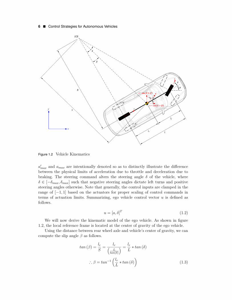
Figure 1.2 Vehicle Kinematics
a′max and amax are intentionally denoted so as to distinctly illustrate the differencebetween the physical limits of acceleration due to throttle and deceleration due tobraking. The steering command alters the steering angle δ of the vehicle, whereδ ∈ [−δmax, δmax] such that negative steering angles dictate left turns and positivesteering angles otherwise. Note that generally, the control inputs are clamped in therange of [−1, 1] based on the actuators for proper scaling of control commands interms of actuation limits. Summarizing, ego vehicle control vector u is defined asfollows.
u = [a, δ]T (1.2)
We will now derive the kinematic model of the ego vehicle. As shown in figure1.2, the local reference frame is located at the center of gravity of the ego vehicle.
Using the distance between rear wheel axle and vehicle’s center of gravity, we cancompute the slip angle β as follows.
tan (β) = lrS
= lr(L
tan(δ)
) = lrL∗ tan (δ)
∴ β = tan−1(lrL∗ tan (δ)
)(1.3)
Control Strategies for Autonomous Vehicles � 7
Ideally, lr = L/2⇒ β = tan−1(tan (δ)
2
)Resolving the velocity vector v into x and y components using the laws of
trigonometry we get,
x = v ∗ cos (θ + β) (1.4)
y = v ∗ sin (θ + β) (1.5)
In order to compute θ, we first need to calculate S using the following relation.
S = L
tan (δ) (1.6)
Using S obtained from equation 1.6, we can compute R as given below.
R = S
cos (β) = L
(tan (δ) ∗ cos (β)) (1.7)
Using R obtained from equation 1.7, we can deduce θ as follows.
θ = v
R= v ∗ tan (δ) ∗ cos (β)
L(1.8)
Finally, we can compute v using the rudimentary differential relation.
v = a (1.9)
Using equations 1.4, 1.5, 1.8 and 1.9, we can formulate the continuous-time kine-matic model of autonomous vehicle.
q =
xy
θv
=
v ∗ cos (θ + β)v ∗ sin (θ + β)v∗tan(δ)∗cos(β)
L
a
(1.10)
Based on the formulation in equation 1.10, we can formulate the discrete-timemodel of autonomous vehicle.
xt+1 = xt + xt ∗∆tyt+1 = yt + yt ∗∆tθt+1 = θt + θt ∗∆tvt+1 = vt + vt ∗∆t
(1.11)
Note that the equation 1.11 is known as the state transition equation (generallyrepresented as qt+1 = qt + qt ∗ ∆t) where t in the subscript denotes current timeinstant and t+ 1 in the subscript denotes next time instant.
8 � Control Strategies for Autonomous Vehicles
1.2.2 Dynamic Model
Dynamics is the study of motion of a system with regard to the forces and torquesthat govern it. In other words, dynamic models are motion models of a system thatclosely resemble the actual system dynamics. Such models tend to be more complexand inefficient to solve in real-time (depends on computational hardware) but aremuch of a requirement for high-performance scenarios such as racing, where drivingat high speeds and with aggressive maneuvers is common.
There are two popular methodologies for formulating dynamic model of systemsviz. Newton-Euler method and Lagrange method. In Newton-Euler approach, one hasto consider all the forces and torques acting on the system, whereas in the Lagrangeapproach, the forces and torques are represented in terms of potential and kineticenergies of the system. It is to be noted that both approaches are equally correct andresult in equivalent formulation of dynamic models. In this section, we will presentlongitudinal and lateral dynamic models of an autonomous vehicle using Newton-Euler approach.
1.2.2.1 Longitudinal Vehicle Dynamics
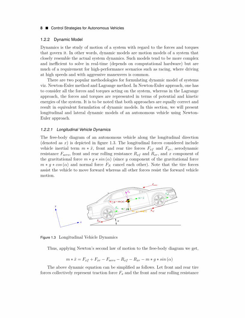
The free-body diagram of an autonomous vehicle along the longitudinal direction(denoted as x) is depicted in figure 1.3. The longitudinal forces considered includevehicle inertial term m ∗ x, front and rear tire forces Fxf and Fxr, aerodynamicresistance Faero, front and rear rolling resistance Rxf and Rxr, and x component ofthe gravitational force m ∗ g ∗ sin (α) (since y component of the gravitational forcem ∗ g ∗ cos (α) and normal force FN cancel each other). Note that the tire forcesassist the vehicle to move forward whereas all other forces resist the forward vehiclemotion.
Figure 1.3 Longitudinal Vehicle Dynamics
Thus, applying Newton’s second law of motion to the free-body diagram we get,
m ∗ x = Fxf + Fxr − Faero −Rxf −Rxr −m ∗ g ∗ sin (α)
The above dynamic equation can be simplified as follows. Let front and rear tireforces collectively represent traction force Fx and the front and rear rolling resistance
Control Strategies for Autonomous Vehicles � 9
collectively represent net rolling resistance Rx. Also, making a small angle approxi-mation for α, we can say that sin (α) ≈ α. Therefore we have,
m ∗ x = Fx − Faero −Rx −m ∗ g ∗ α
∴ x = Fxm− Faero
m− Rx
m− g ∗ α (1.12)
The individual forces can be modeled as follows.
• Traction force Fx depends upon vehicle mass m, wheel radius rwheel andangular acceleration of the wheel θwheel. Since F = m ∗ a and a = r ∗ θ, wehave,
Fx = m ∗ rwheel ∗ θwheel (1.13)
• Aerodynamic resistance Faero depends upon air density ρ, frontal surfacearea of the vehicle A and velocity of the vehicle v. Using proportionality con-stant Cα we have,
Faero = 12 ∗ Cα ∗ ρ ∗ A ∗ v
2 ≈ Cα ∗ v2 (1.14)
• Rolling resistance Rx depends upon tire normal force N , tire pressure P andvelocity of the vehicle v. Note that tire pressure is a function of vehicle velocity.
Rx = N ∗ P (v)
Where, P (v) = Cr,0 + Cr,1 ∗ |v|+ Cr,2 ∗ v2
∴ Rx = N ∗(Cr,0 + Cr,1 ∗ |v|+ Cr,2 ∗ v2
)≈ Cr,1 ∗ |v| (1.15)
Substituting equations 1.13, 1.14 and 1.15 in equation 1.12 we get,
x = rwheel ∗ θwheel −Cα ∗ v2
m− Cr,1 ∗ |v|
m− g ∗ α (1.16)
We can represent the second time derivative of velocity as jerk (rate of change ofacceleration) as follows.
v = j (1.17)
10 � Control Strategies for Autonomous Vehicles
1.2.2.2 Lateral Vehicle Dynamics
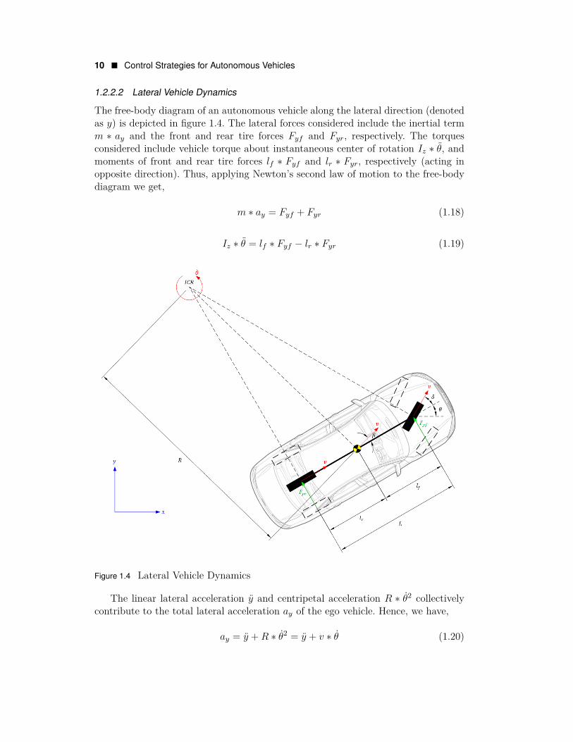
The free-body diagram of an autonomous vehicle along the lateral direction (denotedas y) is depicted in figure 1.4. The lateral forces considered include the inertial termm ∗ ay and the front and rear tire forces Fyf and Fyr, respectively. The torquesconsidered include vehicle torque about instantaneous center of rotation Iz ∗ θ, andmoments of front and rear tire forces lf ∗ Fyf and lr ∗ Fyr, respectively (acting inopposite direction). Thus, applying Newton’s second law of motion to the free-bodydiagram we get,
m ∗ ay = Fyf + Fyr (1.18)
Iz ∗ θ = lf ∗ Fyf − lr ∗ Fyr (1.19)
Figure 1.4 Lateral Vehicle Dynamics
The linear lateral acceleration y and centripetal acceleration R ∗ θ2 collectivelycontribute to the total lateral acceleration ay of the ego vehicle. Hence, we have,
ay = y +R ∗ θ2 = y + v ∗ θ (1.20)
Control Strategies for Autonomous Vehicles � 11
Substituting equation 1.20 into equation 1.18 we get,
m ∗(y + v ∗ θ
)= Fyf + Fyr (1.21)
The linearized lateral tire forces Fyf and Fyr, also known as cornering forces, canbe modeled using front and rear tire slip angles αf and αr, and cornering stiffness offront and rear tires Cf and Cr as follows.Fyf = Cf ∗ αf = Cf ∗
(δ − β − lf∗θ
v
)Fyr = Cr ∗ αr = Cr ∗
(−β + lr∗θ
v
) (1.22)
Substituting the values of linearized lateral tire forces Fyf and Fyr from equation1.22 into equations 1.21 and 1.19 respectively, and rearranging the terms we get,
y = −(Cf + Cr)m
∗ β +(Cr ∗ lr − Cf ∗ lf
m ∗ v− v
)∗ θ + Cf
m∗ δ (1.23)
θ = Cr ∗ lr − Cf ∗ lfIz
∗ β −Cr ∗ l2r + Cf ∗ l2f
Iz ∗ v∗ θ + Cf ∗ lf
Iz∗ δ (1.24)
1.2.2.3 Consolidated Dynamic Model
Equations 1.16, 1.17, 1.23 and 1.24 represent the dynamic model of an autonomousvehicle. The consolidated continuous-time dynamic model of the autonomous vehiclecan be therefore formulated as follows.
q =
xy
θv
=
rwheel ∗ θwheel − Cα∗v2
m − Cr,1∗|v|m − g ∗ α
− (Cf+Cr)m ∗ β +
(Cr∗lr−Cf∗lf
m∗v − v)∗ θ + Cf
m ∗ δCr∗lr−Cf∗lf
Iz∗ β − Cr∗l2r+Cf∗l2f
Iz∗v ∗ θ + Cf∗lfIz∗ δ
j
(1.25)
Based on the formulation in equations 1.25 and 1.10, we can formulate thediscrete-time model of autonomous vehicle as follows.
xt+1 = xt + xt ∗∆t+ xt ∗ ∆t22
yt+1 = yt + yt ∗∆t+ yt ∗ ∆t22
θt+1 = θt + θt ∗∆t+ θt ∗ ∆t22
vt+1 = vt + vt ∗∆t+ vt ∗ ∆t22
(1.26)
Note that the equation 1.26 is known as the state transition equation (generallyrepresented as qt+1 = qt + qt ∗∆t+ qt ∗ ∆t2
2 ) where t in the subscript denotes currenttime instant and t+ 1 in the subscript denotes next time instant.
12 � Control Strategies for Autonomous Vehicles
1.3 CONTROL STRATEGIES
Thus far, we have discussed in detail, all the background concepts related to controlstrategies for autonomous vehicles (or any other system for that matter).
In this section we present classical as well as some of the current state-of-the-art control strategies for autonomous vehicles. Some of these are pretty easy andintuitive, while others are not. We shall begin discussing simpler ones first and thenintroduce more complex strategies for vehicle control, but first, let us see the differentcontrol schemes.
1.3.1 Control Schemes
As stated in section 1.1.3, the control system of an autonomous vehicle is split intolongitudinal and lateral components. Depending on whether or not these componentsinfluence each other, the control schemes can be referred to as coupled or de-coupledcontrol.
1.3.1.1 Coupled Control
Coupled control refers to a control scheme wherein the lateral and longitudinal con-trollers operate synergistically and have some form of influence over each other. Al-though this approach is very much realistic, the major difficulty in practical imple-mentation lies in accurately determining the “amount” of influence the controllers aresupposed to have over one another considering the motion model and the operationaldesign domain (ODD) of the ego vehicle.
In coupled-control scheme, the lateral controller may influence the longitudinalcontroller or vice-versa, or both may have an influence over each other. Let us considereach case independently with an example.
Longitudinal Controller Influencing Lateral Controller
In this case, the longitudinal controller is dominant or has a higher preferenceover the lateral controller. As a result, the longitudinal control action is computedindependently, and this influences the lateral control action with an inverse relation(i.e. inverse proportionality). Since it is not a good idea to have a large steering angleat high speed, the controller regulates maximum steering limit inversely proportionalto the vehicle speed.
Lateral Controller Influencing Longitudinal Controller
As opposed to the previous case, in this one, the lateral controller is dominantor has a higher preference over the longitudinal controller. As a result, the lateralcontrol action is computed independently, and this influences the longitudinal controlaction with an inverse relation (i.e. inverse proportionality). Since it is a bad idea tohave high speed with large steering angle, the controller regulates maximum speedlimit inversely proportional to the steering angle.
Control Strategies for Autonomous Vehicles � 13
Longitudinal and Lateral Controllers Influencing Each Other
In this case, both the controllers tend to influence each other depending uponthe operating conditions. If it is more important to maintain high speeds, the longi-tudinal controller has a higher (more dominant) influence over the lateral controllerand if the maneuver requires cornering at sharp turns, the lateral controller has ahigher (more dominant) influence over the longitudinal controller. Generally, the op-erating conditions change over the coarse of duration and “weights” need to be shiftedin order to switch the dominance of lateral and longitudinal controllers.
1.3.1.2 De-Coupled Control
De-coupled control refers to a control scheme wherein the lateral and longitudinalcontrollers do not have any influence on each other, i.e. both the controllers operateindependently disregarding the control actions generated by other.
Although this simplifies the control problem to a large extent, this type of controlscheme does not seem much realistic considering the fact that lateral and longitudinalvehicle dynamics inherently affect each other. In other words, this control scheme isapplicable to highly specific and uniform driving scenarios (i.e. limited ODD).
1.3.2 Traditional Control
Traditional control is one of the most widely used and reliable control strategy, es-pecially when it comes to safety-critical systems such as autonomous vehicles.
There are primarily three objectives of a controller.
1. Stability: Stability refers to the fact that a system should always produce abounded output (response) when excited with a bounded input signal. This cri-terion for stability is popularly known as the BIBO criterion. This is especiallysignificant for inherently unstable systems.
2. Tracking: Tracking refers to the fact that a control system should be able totrack the desired reference value (a.k.a. setpoint). In other words, the systemresponse should be as close to the setpoint as possible, with minimal transientand/or steady state error (zero in ideal case).
3. Robustness: Robustness refers to the fact that a control system should beable to exhibit stability and tracking despite external disturbances. In otherwords, the system must remain stable (i.e. meet the BIBO criterion) and itsresponse should be as close to the setpoint as possible even when it is disturbedby external factors.
Since traditional controllers can be tuned and analyzed to meet the objectivesstated above, they become the primary choice of control strategies, especially forsystems such as autonomous robots and vehicles.
Traditional control systems can either be open loop, which do not use any statefeedback or closed loop, which do. However, when it comes to motion control of
14 � Control Strategies for Autonomous Vehicles
autonomous vehicles, a control problem where operating conditions are continuouslychanging, open loop control is not a possibility. Thus, for control of autonomousvehicles, closed loop control systems are implemented with an assumption that thestate is directly measurable or can be estimated by implementing state observers. Suchtraditional controllers can be classified as model-free and model-based controllers.
1. Model-Free Controllers: These type of controllers do not use any mathemat-ical model of the system being controlled. They tend to take “corrective” actionbased on the “error” between setpoint and current state. These controllers arequite easy to implement since they do not require in-depth knowledge of thebehavior of the system, however, are difficult to tune, do not guarantee opti-mal performance and perform satisfactorily under limited operating conditions.Common examples of these type of controllers include bang-bang controllers,PID controllers, intelligent PID controllers (iPIDs), etc.
2. Model-Based Controllers: These type of controllers use some or the othertype of mathematical model of the system being controlled. Depending uponthe model complexity and the exact approach followed to generate the controlcommands, these can be further classified as follows.
(a) Kinematic Controllers: These type of controllers use simplified motionmodels of the system and are based on the geometry and kinematics of thesystem (generally employing first order approximation). They assume noslip, no skip and often ignore internal or external forces acting on the sys-tem. Therefore, these type of controllers are often restricted to low-speedapplications (where system dynamics can be approximated), but offer anadvantage of low computational complexity (which is extremely signifi-cant in real-world implementation as opposed to theoretical formulationor simulation).
(b) Dynamic Controllers: These type of controllers use detailed motionmodels of the system and are based on system dynamics. They considerforces and torques acting on the system as well as any disturbances (in-corporated in the dynamic model). Therefore, these type of controllershave an upper hand when compared to kinematic controllers due to theunrestricted ODD, but suffer higher computational complexity owing tothe complex computations involving detailed models at each time step.
(c) Model Predictive Controllers: These type of controllers use linear ornon-linear motion models of the system to predict its future states (upto a finite receding horizon) and determine the optimal control action bynumerically solving a bounded optimization problem at each time step(essentially treating the control problem as an optimization problem, astrategy known as optimal control). The optimization problem is boundedsince model predictive controllers explicitly handle motion constraints,which is another reason for their popularity. Although this sounds to bethe perfect control strategy, it is to be noted that since model predictive
Control Strategies for Autonomous Vehicles � 15
controllers use complex motion models and additionally solve an onlineoptimization problem at each time step, they are computationally expen-sive and may cause undesirable control latency (sometimes even of theorder of a few seconds) if not implemented wisely.
The upcoming sections discuss these traditional control strategies for autonomousvehicles in a greater detail.
1.3.2.1 Bang-Bang Control
The bang-bang controller is a simple binary controller. It is extremely easy to im-plement, which is the most significant (and perhaps the only) reason for adoptingit. The control action u is switched between two states umax and umin (analogous toon/off, high/low, true/false, set/reset, 1/0, etc.) based on whether the input signal xis above or below the reference value xref .
u ={umax ;x < xref
umin ;x > xref
Note that a multi-step controller may be adopted to switch the control actionbased on more than just two cases. For example, a third control action of 0 is alsopossible in case the error becomes exactly zero (i.e. x = xref ); however, practically,this case will sustain only instantaneously, since even a small error value will overshootthe system response.
The bang-bang controller, in either of its two states, generates the same controlaction regardless of the error value. In other words, it does not account for themagnitude of error signal. It is, therefore, termed as “unstable” due to its abruptresponses, and is recommended to be applied only to variable structure systems (VSS)that allow sliding motion control (SMC).
Considering the final control elements (throttle, brake and steering) of an au-tonomous vehicle, it is safe to say that bang-bang controller may not be applied tocontrol the lateral vehicle dynamics; the vehicle would constantly oscillate about themean position, trying to minimize the cross-track error e∆ and/or heading error eψ bycompletely turning the steering wheel in one direction or the other, which would benot only uncomfortable but also dangerous and may even cause a rollover at highervelocities. Nonetheless, bang-bang controller may be applied to control the longitudi-nal vehicle dynamics by fully actuating the throttle and brakes based on the velocityerror ev and while this may be safe, it may still result in exceeding the nominal jerkvalues, causing a rather uncomfortable ride. It is important to note at this point thatabrupt control actions generated by a bang-bang controller can possibly cause lifetimereduction, if not immediate breakdown, of actuators, which is highly undesirable.
Bang-Bang Control Implementation
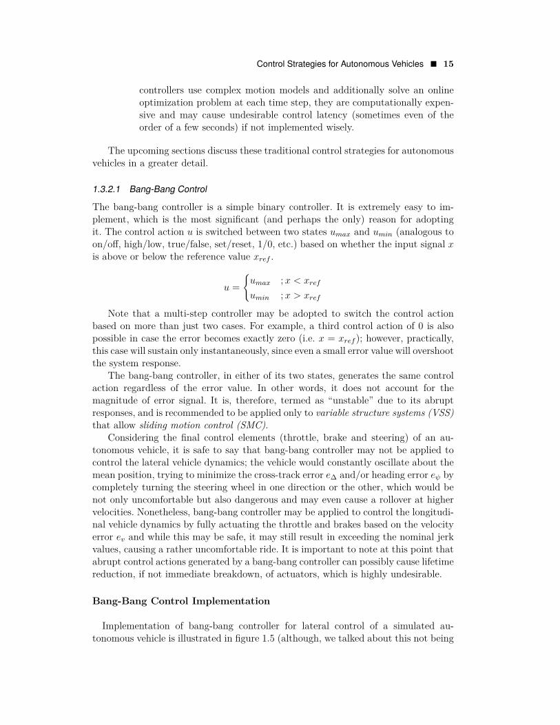
Implementation of bang-bang controller for lateral control of a simulated au-tonomous vehicle is illustrated in figure 1.5 (although, we talked about this not being

16 � Control Strategies for Autonomous Vehicles
Figure 1.5 Bang-Bang Control Implementation
a good idea). In order to have uniformity across all the implementations discussedin this chapter, a well-tuned PID controller was employed for longitudinal control ofthe ego vehicle.
For the purpose of this implementation, the reference trajectory to be followed bythe ego vehicle (marked green in the trajectory plot) was discretized into waypointsto be tracked by the lateral controller, and each waypoint had an associated velocitysetpoint to be tracked by the longitudinal controller.
The bang-bang controller response was alleviated by multiplying the control ac-tion with a limiting factor of 0.1, thereby restricting the steering actuation limitδ ∈ [−7◦, 7◦]. This allowed the bang-bang controller to track the waypoints at leastfor a while, after which, the ego vehicle went out of control and crashed!
The steering commands generated by the bang-bang controller are worth noting.
Control Strategies for Autonomous Vehicles � 17
It can be clearly seen how the controller switches back-and-forth between the twoextremities, and although it was programmed to produce no control action (i.e. 0)when the cross-track error was negligible, such an incident never occurred during thecourse of simulation.
In reality, it is the abrupt control actions that quickly render the plant uncon-trollable, which implies that the controller harms itself. Furthermore, it is to benoted that generating such abrupt control actions may not be possible practically,since the actuators have a finitely positive time-constant (especially steering actu-ation mechanism), and that doing so may cause serious damage to the actuationelements (especially at high frequencies, such as those observed between time-steps15-25). This fact further adds to the controlability problem, rendering the bang-bangcontroller close to useless for controlling the lateral vehicle dynamics.
1.3.2.2 PID Control
From the previous discussion, it is evident that bang-bang controller is not a verypromising option for vehicle control (especially lateral control, but also not so goodfor longitudinal control either) and better control strategies are required.
P Controller
The most intuitive upgrade from bang-bang controller is the proportional (P) con-troller. The P controller generates a control action u proportional to the error signale, and the proportionality constant that scales the control action is called gain of theP controller (generally denoted as kP ).
In continuous time, the P controller is represented as follows.
u(t) = kP ∗ e(t)
In discrete time, the above equation takes the following form.
ut+1 = kP ∗ etIt is extremely important to tune the gain value so as to obtain a desired system
response. A low gain value would increase the settling time of the system drastically,whereas a high gain value would overshoot the system in the opposite direction.A moderate proportional gain would try to minimize the error, however, being anerror-driven controller, it would still leave behind a significantly large steady-stateerror.
PD Controller
The PD controller can be thought of as a compound controller constituted of theproportional (P) and derivative (D) controllers.
The P component of the PD controller, as stated earlier, produces a “surrogate”
18 � Control Strategies for Autonomous Vehicles
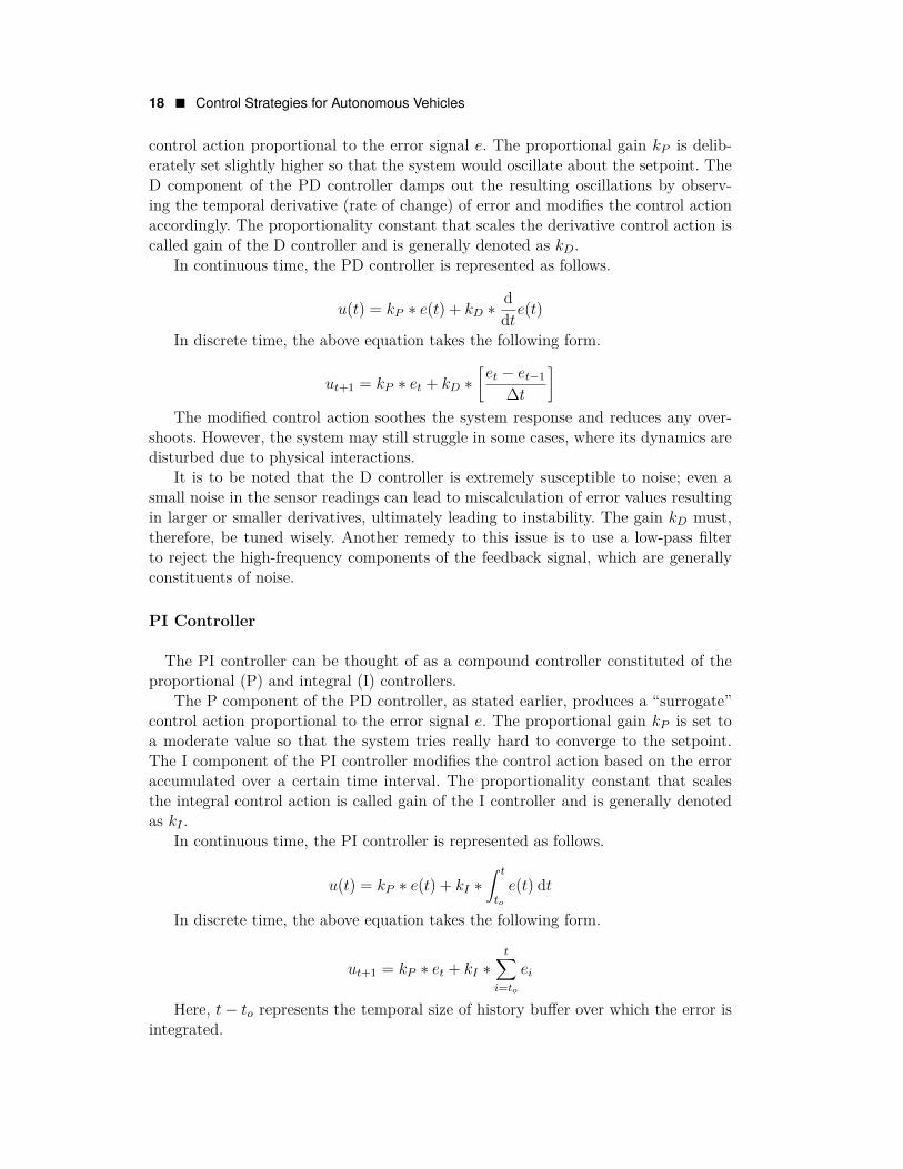
control action proportional to the error signal e. The proportional gain kP is delib-erately set slightly higher so that the system would oscillate about the setpoint. TheD component of the PD controller damps out the resulting oscillations by observ-ing the temporal derivative (rate of change) of error and modifies the control actionaccordingly. The proportionality constant that scales the derivative control action iscalled gain of the D controller and is generally denoted as kD.
In continuous time, the PD controller is represented as follows.
u(t) = kP ∗ e(t) + kD ∗ddte(t)
In discrete time, the above equation takes the following form.
ut+1 = kP ∗ et + kD ∗[et − et−1
∆t
]The modified control action soothes the system response and reduces any over-
shoots. However, the system may still struggle in some cases, where its dynamics aredisturbed due to physical interactions.
It is to be noted that the D controller is extremely susceptible to noise; even asmall noise in the sensor readings can lead to miscalculation of error values resultingin larger or smaller derivatives, ultimately leading to instability. The gain kD must,therefore, be tuned wisely. Another remedy to this issue is to use a low-pass filterto reject the high-frequency components of the feedback signal, which are generallyconstituents of noise.
PI Controller
The PI controller can be thought of as a compound controller constituted of theproportional (P) and integral (I) controllers.
The P component of the PD controller, as stated earlier, produces a “surrogate”control action proportional to the error signal e. The proportional gain kP is set toa moderate value so that the system tries really hard to converge to the setpoint.The I component of the PI controller modifies the control action based on the erroraccumulated over a certain time interval. The proportionality constant that scalesthe integral control action is called gain of the I controller and is generally denotedas kI .
In continuous time, the PI controller is represented as follows.
u(t) = kP ∗ e(t) + kI ∗∫ t
to
e(t) dt
In discrete time, the above equation takes the following form.
ut+1 = kP ∗ et + kI ∗t∑
i=toei
Here, t− to represents the temporal size of history buffer over which the error isintegrated.
Control Strategies for Autonomous Vehicles � 19
The modified control action forces the overall system response to get much closerto the setpoint value as the time proceeds. In other words, it helps the system betterconverge to the desired value. It is also worth mentioning that the I component isalso effective in dealing with any systematic biases, such as inherent misalignments,disturbance forces, etc. However, with a simple PI controller implemented, the systemmay tend to overshoot every time a control action is executed.
It is to be noted that since the I controller acts on the accumulated error, whichis a large value, its gain kI is usually set very low.
PID Controller
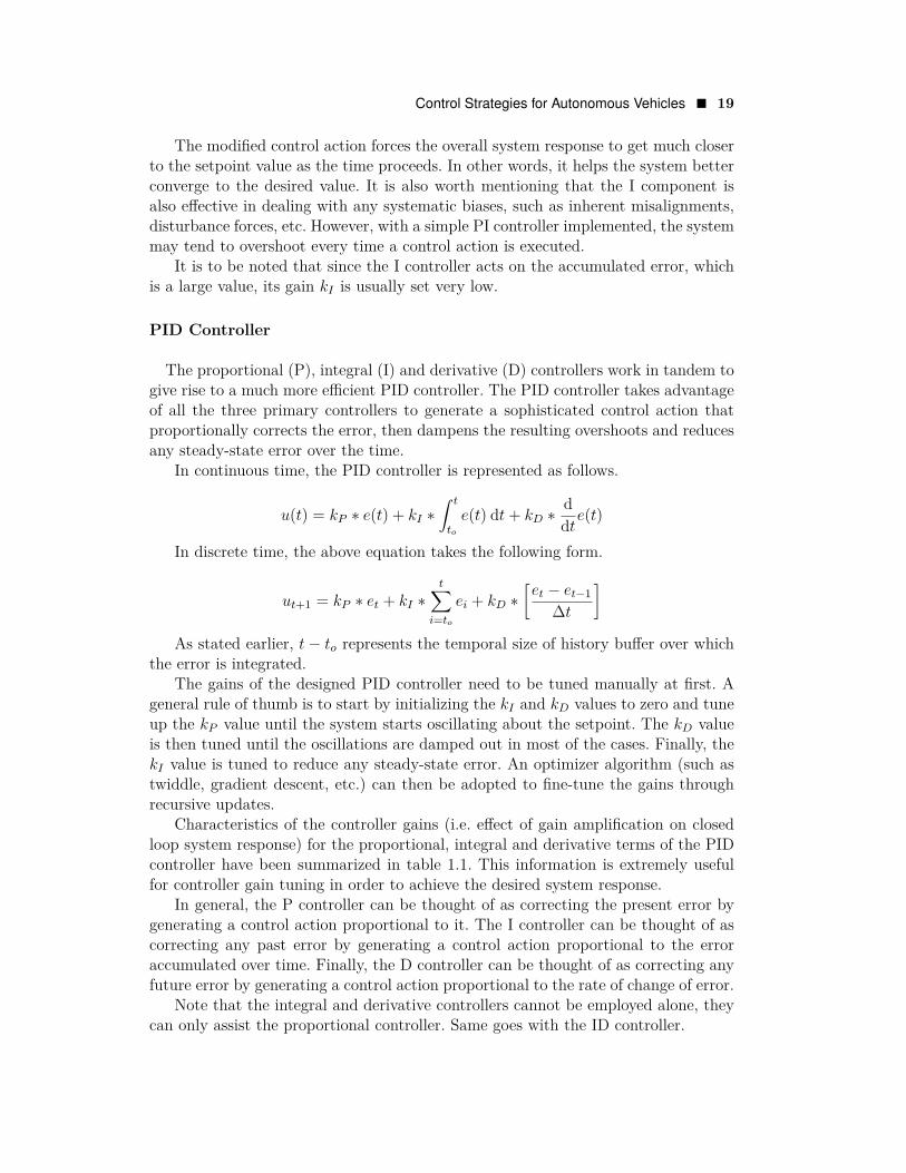
The proportional (P), integral (I) and derivative (D) controllers work in tandem togive rise to a much more efficient PID controller. The PID controller takes advantageof all the three primary controllers to generate a sophisticated control action thatproportionally corrects the error, then dampens the resulting overshoots and reducesany steady-state error over the time.
In continuous time, the PID controller is represented as follows.
u(t) = kP ∗ e(t) + kI ∗∫ t
to
e(t) dt+ kD ∗ddte(t)
In discrete time, the above equation takes the following form.
ut+1 = kP ∗ et + kI ∗t∑
i=toei + kD ∗
[et − et−1
∆t
]As stated earlier, t− to represents the temporal size of history buffer over which
the error is integrated.The gains of the designed PID controller need to be tuned manually at first. A
general rule of thumb is to start by initializing the kI and kD values to zero and tuneup the kP value until the system starts oscillating about the setpoint. The kD valueis then tuned until the oscillations are damped out in most of the cases. Finally, thekI value is tuned to reduce any steady-state error. An optimizer algorithm (such astwiddle, gradient descent, etc.) can then be adopted to fine-tune the gains throughrecursive updates.
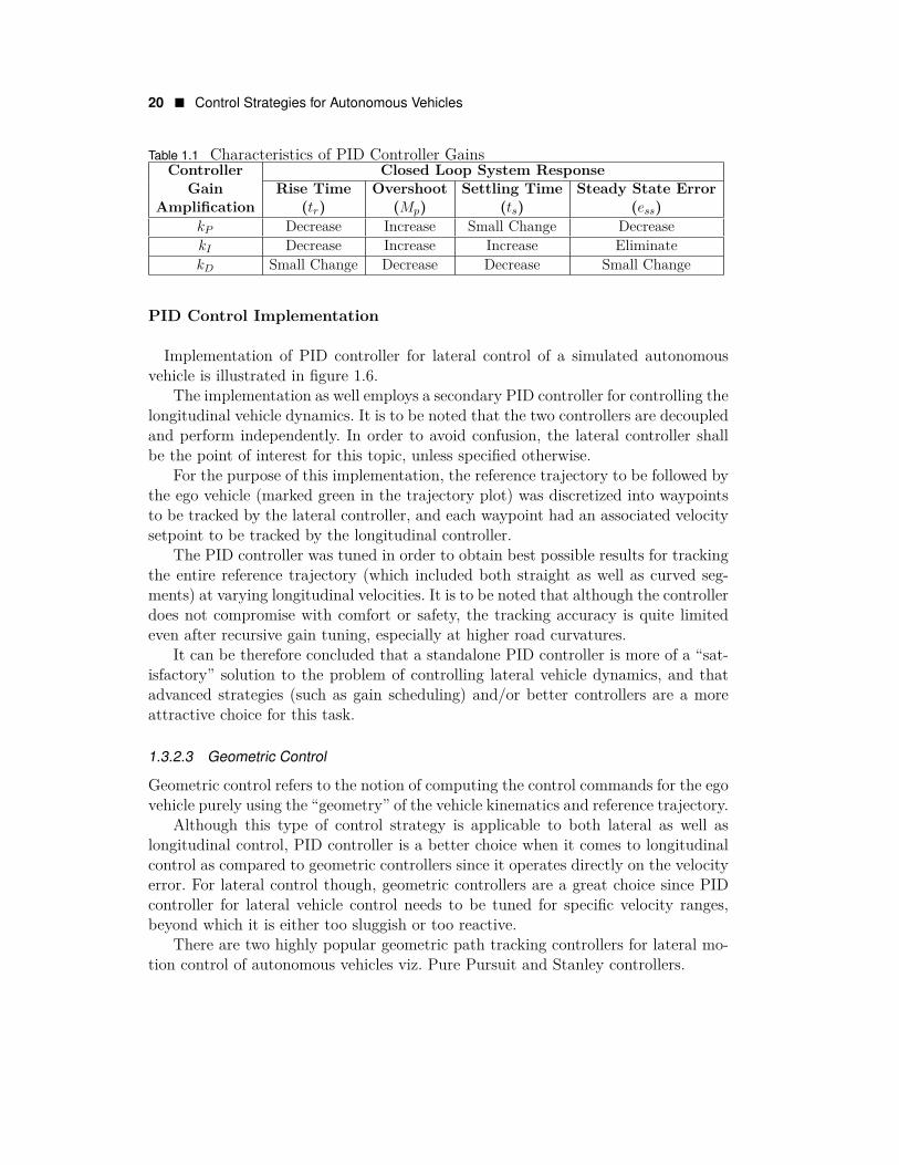
Characteristics of the controller gains (i.e. effect of gain amplification on closedloop system response) for the proportional, integral and derivative terms of the PIDcontroller have been summarized in table 1.1. This information is extremely usefulfor controller gain tuning in order to achieve the desired system response.
In general, the P controller can be thought of as correcting the present error bygenerating a control action proportional to it. The I controller can be thought of ascorrecting any past error by generating a control action proportional to the erroraccumulated over time. Finally, the D controller can be thought of as correcting anyfuture error by generating a control action proportional to the rate of change of error.
Note that the integral and derivative controllers cannot be employed alone, theycan only assist the proportional controller. Same goes with the ID controller.
20 � Control Strategies for Autonomous Vehicles
Table 1.1 Characteristics of PID Controller GainsController
GainAmplification
Closed Loop System ResponseRise Time
(tr)Overshoot
(Mp)Settling Time
(ts)Steady State Error
(ess)kP Decrease Increase Small Change DecreasekI Decrease Increase Increase EliminatekD Small Change Decrease Decrease Small Change
PID Control Implementation
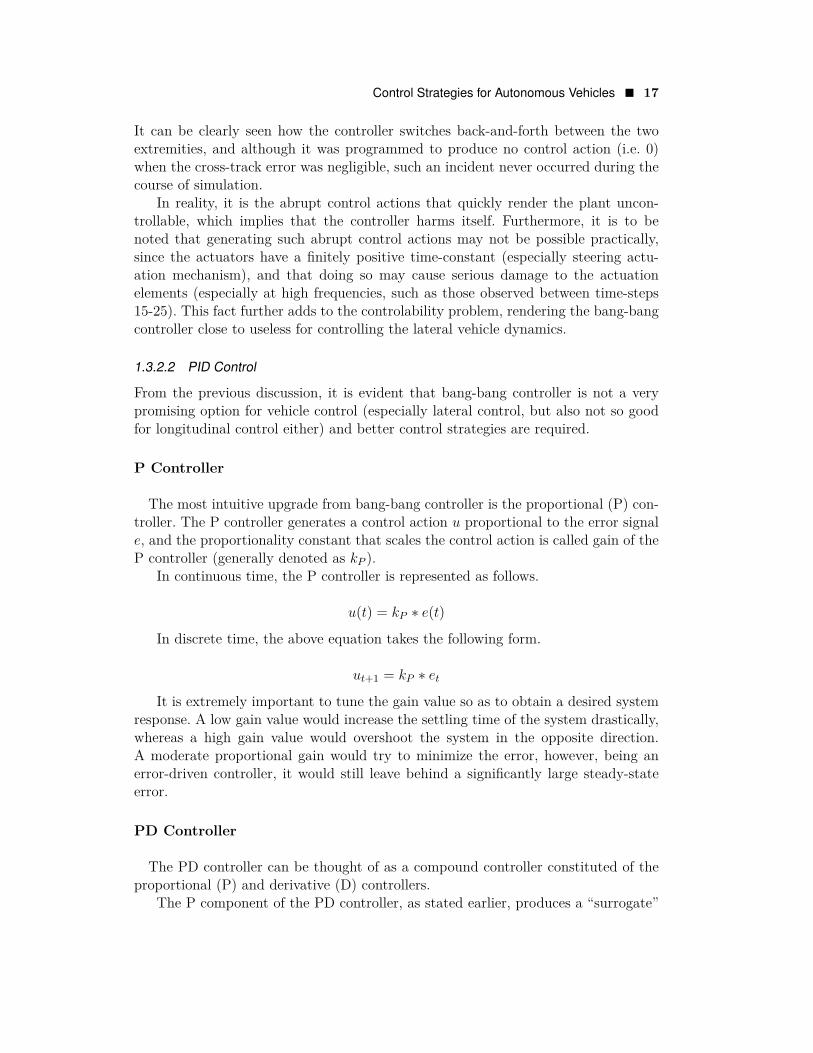
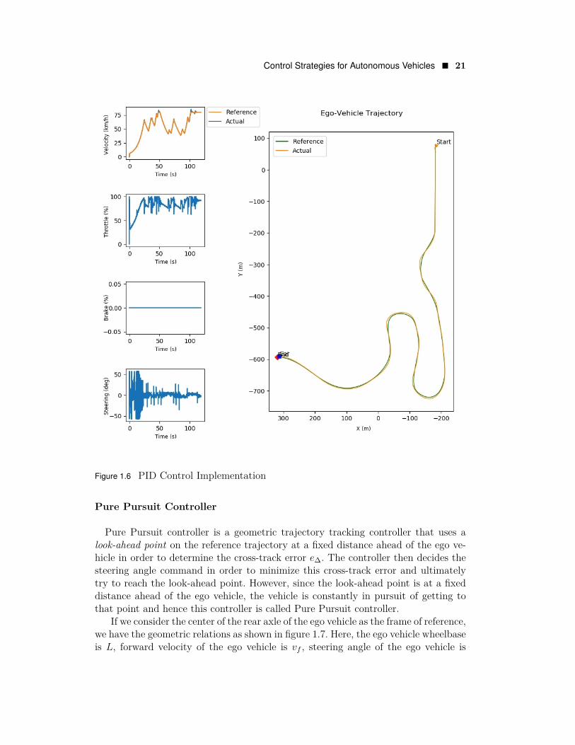
Implementation of PID controller for lateral control of a simulated autonomousvehicle is illustrated in figure 1.6.
The implementation as well employs a secondary PID controller for controlling thelongitudinal vehicle dynamics. It is to be noted that the two controllers are decoupledand perform independently. In order to avoid confusion, the lateral controller shallbe the point of interest for this topic, unless specified otherwise.
For the purpose of this implementation, the reference trajectory to be followed bythe ego vehicle (marked green in the trajectory plot) was discretized into waypointsto be tracked by the lateral controller, and each waypoint had an associated velocitysetpoint to be tracked by the longitudinal controller.
The PID controller was tuned in order to obtain best possible results for trackingthe entire reference trajectory (which included both straight as well as curved seg-ments) at varying longitudinal velocities. It is to be noted that although the controllerdoes not compromise with comfort or safety, the tracking accuracy is quite limitedeven after recursive gain tuning, especially at higher road curvatures.
It can be therefore concluded that a standalone PID controller is more of a “sat-isfactory” solution to the problem of controlling lateral vehicle dynamics, and thatadvanced strategies (such as gain scheduling) and/or better controllers are a moreattractive choice for this task.
1.3.2.3 Geometric Control
Geometric control refers to the notion of computing the control commands for the egovehicle purely using the “geometry” of the vehicle kinematics and reference trajectory.
Although this type of control strategy is applicable to both lateral as well aslongitudinal control, PID controller is a better choice when it comes to longitudinalcontrol as compared to geometric controllers since it operates directly on the velocityerror. For lateral control though, geometric controllers are a great choice since PIDcontroller for lateral vehicle control needs to be tuned for specific velocity ranges,beyond which it is either too sluggish or too reactive.
There are two highly popular geometric path tracking controllers for lateral mo-tion control of autonomous vehicles viz. Pure Pursuit and Stanley controllers.
Control Strategies for Autonomous Vehicles � 21
Figure 1.6 PID Control Implementation
Pure Pursuit Controller
Pure Pursuit controller is a geometric trajectory tracking controller that uses alook-ahead point on the reference trajectory at a fixed distance ahead of the ego ve-hicle in order to determine the cross-track error e∆. The controller then decides thesteering angle command in order to minimize this cross-track error and ultimatelytry to reach the look-ahead point. However, since the look-ahead point is at a fixeddistance ahead of the ego vehicle, the vehicle is constantly in pursuit of getting tothat point and hence this controller is called Pure Pursuit controller.
If we consider the center of the rear axle of the ego vehicle as the frame of reference,we have the geometric relations as shown in figure 1.7. Here, the ego vehicle wheelbaseis L, forward velocity of the ego vehicle is vf , steering angle of the ego vehicle is
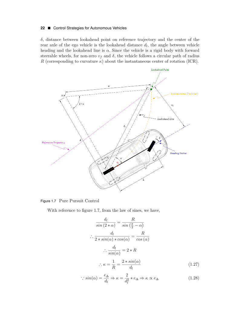
22 � Control Strategies for Autonomous Vehicles
δ, distance between lookahead point on reference trajectory and the center of therear axle of the ego vehicle is the lookahead distance dl, the angle between vehicleheading and the lookahead line is α. Since the vehicle is a rigid body with forwardsteerable wheels, for non-zero vf and δ, the vehicle follows a circular path of radiusR (corresponding to curvature κ) about the instantaneous center of rotation (ICR).
Figure 1.7 Pure Pursuit Control
With reference to figure 1.7, from the law of sines, we have,
dlsin (2 ∗ α) = R
sin(π2 − α
)∴
dl2 ∗ sin(α) ∗ cos(α) = R
cos (α)
∴dl
sin(α) = 2 ∗R
∴ κ = 1R
= 2 ∗ sin(α)dl
(1.27)
∵ sin(α) = e∆
dl⇒ κ = 2
d2l
∗ e∆ ⇒ κ ∝ e∆ (1.28)
Control Strategies for Autonomous Vehicles � 23
It can be seen from equation 1.28 that curvature of the instantaneous trajectoryκ is directly proportional to the cross-track error e∆. Thus, as the cross-track errorincreases, so does the trajectory curvature, thereby bringing the vehicle back towardsthe reference trajectory aggressively. Note that the term 2
d2l
can be thought of as aproportionality gain, which can be tuned based on the lookahead distance parameter.
With reference to figure 1.7, the steering angle command δ can be computed usingthe following relation.
tan(δ) = L
R= L ∗ κ (1.29)
Substituting the value of κ from equation 1.27 in equation 1.29 and solving for δwe get,
δ = tan−1(2 ∗ L ∗ sin(α)
dl
)(1.30)
Equation 1.30 presents the de-coupled scheme of Pure Pursuit controller (i.e. thesteering law is independent of vehicle velocity). As a result, if the controller is tunedfor low speed, it will be dangerously aggressive at higher speeds while if tuned forhigh speed, the controller will be too sluggish at lower speeds. One potentially simpleimprovement would be to vary the lookahead distance dl proportional to the vehiclevelocity vf using kv as the proportionality constant (this constant/gain will act asthe tuning parameter for Pure Pursuit controller).
dl = kv ∗ vf (1.31)
Substituting the value of dl from equation 1.31 in equation 1.30 we get the com-plete coupled Pure Pursuit control law formulation as follows.
δ = tan−1(
2 ∗ L ∗ sin(α)kv ∗ vf
); δ ∈ [−δmax, δmax] (1.32)
In summary, it can be seen that Pure Pursuit controller acts as a geometricproportional controller of steering angle δ operating on the cross-track error e∆ whileobserving the steering actuation limits.
Pure Pursuit Control Implementation
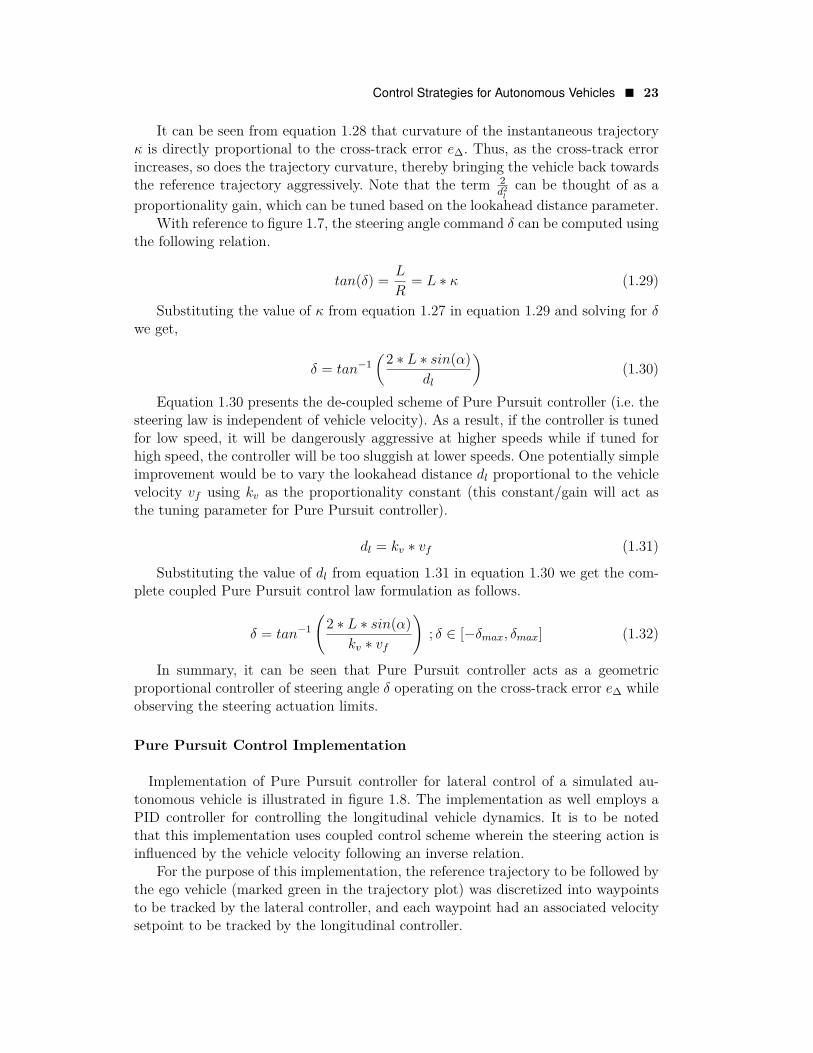
Implementation of Pure Pursuit controller for lateral control of a simulated au-tonomous vehicle is illustrated in figure 1.8. The implementation as well employs aPID controller for controlling the longitudinal vehicle dynamics. It is to be notedthat this implementation uses coupled control scheme wherein the steering action isinfluenced by the vehicle velocity following an inverse relation.
For the purpose of this implementation, the reference trajectory to be followed bythe ego vehicle (marked green in the trajectory plot) was discretized into waypointsto be tracked by the lateral controller, and each waypoint had an associated velocitysetpoint to be tracked by the longitudinal controller.
24 � Control Strategies for Autonomous Vehicles
Figure 1.8 Pure Pursuit Control Implementation
The lateral controller parameter kv was tuned in order to obtain best possibleresults for tracking the entire reference trajectory (which included both straight aswell as curved segments) at varying forward velocities. The controller was very wellable to track the prescribed trajectory with a promising level of precision. Addition-ally, the control actions generated during the entire course of simulation lied withina short span δ ∈ [−15◦, 15◦], which is an indication of the controller having a goodcommand over the system.
Nonetheless, a green highlight (representing the reference trajectory) can be seenin the neighborhood of actual trajectory followed by the ego vehicle, which indicatesthat the tracking was not “perfect”. This may be partially due to the fact that thePure Pursuit control law has a single tunable parameter dl having an approximatedfirst order relation with vf . However, a more convincing reason for potential errors

Control Strategies for Autonomous Vehicles � 25
in trajectory tracking, when it comes to Pure Pursuit controller, is that it generatessteering action regardless of heading error of the vehicle, making it difficult to actuallyalign the vehicle precisely along the reference trajectory.
Furthermore, being a kinematic controller, Pure Pursuit controller disregards ac-tual system dynamics, and as a result compromises with trajectory tracking accuracy.Now, although this may not affect a vehicle driving under nominal conditions, a racingvehicle, for example, would experience serious trajectory deviations under rigorousdriving conditions.
Pure Pursuit controller also has a pretty non-intuitive issue associated with it,which is generally undiscovered during infinitely continuous or looped trajectorytracking. Particularly, towards the end of a finite reference trajectory, the Pure Pur-suit controller generates erratic steering actions owing to the fact that the look-aheadpoint it uses in order to deduce the steering control action is no longer available, sincethe further waypoints are not really defined. This may lead to undesired stoppage ofthe ego vehicle or even cause it to wander off of the trajectory in the final few secondsof the mission.
In conclusion, Pure Pursuit controller is really good for regulating the lateraldynamics of a vehicle operating under nominal driving conditions, and that there isroom for further improvement.
Stanley Controller
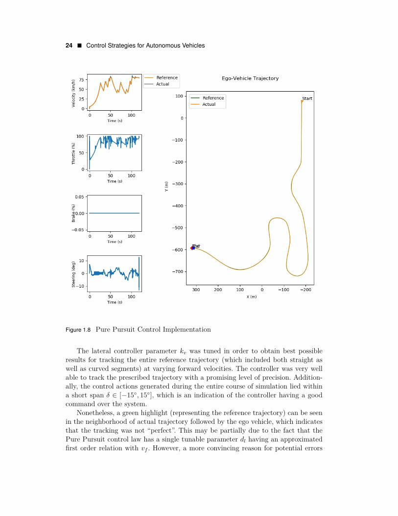
Stanley controller is a geometric trajectory tracking controller developed by Stan-ford University’s “Stanford Racing Team” for their autonomous vehicle “Stanley”at the DARPA Grand Challenge (2005). As opposed to Pure Pursuit controller (dis-cussed earlier), which uses only the cross-track error to determine the steering action,Stanley controller uses both heading as well as cross-track errors to determine thesame. The cross-track error e∆ is defined with respect to a closest point on the refer-ence trajectory (as opposed to a lookahead point in case of Pure Pursuit controller)whereas the heading error eψ is defined using the vehicle heading relative to thereference trajectory.
If we consider the center of the front axle of the ego vehicle as the frame ofreference, we have the geometric relations as shown in figure 1.9. Here, the ego vehiclewheelbase is L, forward velocity of the ego vehicle is vf , and steering angle of the egovehicle is δ.
Stanley controller uses both heading as well as cross-track errors to determine thesteering command. Furthermore, the steering angle generated by this (or any other)method must observe the steering actuation limits. Stanley control law, therefore, isessentially defined to meet the following three requirements.
1. Heading Error Correction: To correct the heading error eψ by producing asteering control action δ proportional (or equal) to it, such that vehicle headingaligns with the desired heading.
δ = eψ (1.33)
26 � Control Strategies for Autonomous Vehicles
Figure 1.9 Stanley Control
2. Cross-Track Error Correction: To correct the cross-track error e∆ by pro-ducing a steering control action δ directly proportional to it and inversely pro-portional to the vehicle velocity vf in order to achieve coupled-control. More-over, the effect for large cross-track errors can be limited by using an inversetangent function.
δ = tan−1(k∆ ∗ e∆
vf
)(1.34)
It is to be noted that at this stage of the formulation, the inverse relationbetween steering angle and vehicle speed can cause numerical instability incontrol actions.At lower speeds, the denominator becomes small, thus causing the steeringcommand to shoot to higher values, which is undesirable considering humancomfort. Hence, an extra softening coefficient ks may be used in the denomi-nator as an additive term in order to keep the steering commands smaller forsmoother steering actions.On the contrary, at higher velocities, the denominator becomes large making the
Control Strategies for Autonomous Vehicles � 27
steering commands small in order to avoid large lateral accelerations. However,even these small steering actions might be high in some cases, causing highlateral accelerations. Hence, an extra damping coefficient kd may be used inorder to dampen the steering action proportional to vehicle velocity.
δ = tan−1(
k∆ ∗ e∆
ks + kd ∗ vf
)(1.35)
3. Clipping Control Action: To continuously observe the steering actuationlimits [−δmax, δmax] and clip the steering command within these bounds.
δ ∈ [−δmax, δmax] (1.36)
Using equations 1.33, 1.35 and 1.36 we can formulate the complete Stanley controllaw as follows.
δ = eψ + tan−1(
k∆ ∗ e∆
ks + kd ∗ vf
); δ ∈ [−δmax, δmax] (1.37)
In summary, it can be seen that Stanley controller acts as a geometric proportionalcontroller of steering angle δ operating on the heading error eψ as well as the cross-track error e∆, while observing the steering actuation limits.
Stanley Control Implementation
Implementation of Stanley controller for lateral control of a simulated autonomousvehicle is illustrated in figure 1.10. The implementation as well employs a PID con-troller for controlling the longitudinal vehicle dynamics. It is to be noted that thisimplementation uses coupled control scheme wherein the steering action is influencedby the vehicle velocity following an inverse relation.
For the purpose of this implementation, the reference trajectory to be followed bythe ego vehicle (marked green in the trajectory plot) was discretized into waypointsto be tracked by the lateral controller, and each waypoint had an associated velocitysetpoint to be tracked by the longitudinal controller.
The lateral controller parameters k∆, ks and kd were tuned in order to obtainbest possible results for tracking the entire reference trajectory (which included bothstraight as well as curved segments) at varying forward velocities. The controller wasable to track the prescribed trajectory with a promising level of precision.
Nonetheless, a slight green highlight (representing the reference trajectory) canbe occasionally spotted in the neighborhood of actual trajectory followed by the egovehicle, which indicates that the tracking was sub-optimal or near-perfect. This maybe due to the first order approximations involved in the formulation. Furthermore,being a kinematic geometric controller, Stanley controller disregards actual systemdynamics, and as a result compromises with trajectory tracking accuracy, especiallyunder rigorous driving conditions.

28 � Control Strategies for Autonomous Vehicles
Figure 1.10 Stanley Control Implementation
Stanley controller uses the closest waypoint to compute the cross-track error,owing to which, it may become highly reactive at times. Since this implementationassumed static waypoints defined along a racetrack (i.e. in the global frame), andthe ego vehicle was spawned towards one side of the track, the initial cross-trackerror was quite high. This made the controller react erratically, thereby generatingsteering commands of over 50◦ in either direction. However, this is not a significantproblem practically, since the local trajectory is recursively planned as a finite set ofwaypoints originating from the vehicle coordinate system, thereby ensuring that theimmediately next waypoint is not too far from the vehicle.
In conclusion, Stanley controller is one of the best for regulating lateral dynamicsof a vehicle operating under nominal driving conditions, especially considering thecomputational complexity at which it offers such accuracy and robustness.
Control Strategies for Autonomous Vehicles � 29
1.3.2.4 Model Predictive Control
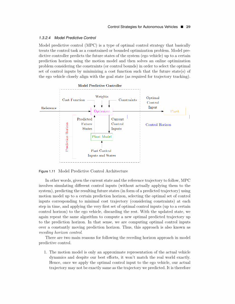
Model predictive control (MPC) is a type of optimal control strategy that basicallytreats the control task as a constrained or bounded optimization problem. Model pre-dictive controller predicts the future states of the system (ego vehicle) up to a certainprediction horizon using the motion model and then solves an online optimizationproblem considering the constraints (or control bounds) in order to select the optimalset of control inputs by minimizing a cost function such that the future state(s) ofthe ego vehicle closely align with the goal state (as required for trajectory tracking).
Figure 1.11 Model Predictive Control Architecture
In other words, given the current state and the reference trajectory to follow, MPCinvolves simulating different control inputs (without actually applying them to thesystem), predicting the resulting future states (in form of a predicted trajectory) usingmotion model up to a certain prediction horizon, selecting the optimal set of controlinputs corresponding to minimal cost trajectory (considering constraints) at eachstep in time, and applying the very first set of optimal control inputs (up to a certaincontrol horizon) to the ego vehicle, discarding the rest. With the updated state, weagain repeat the same algorithm to compute a new optimal predicted trajectory upto the prediction horizon. In that sense, we are computing optimal control inputsover a constantly moving prediction horizon. Thus, this approach is also known asreceding horizon control.
There are two main reasons for following the receding horizon approach in modelpredictive control.
1. The motion model is only an approximate representation of the actual vehicledynamics and despite our best efforts, it won’t match the real world exactly.Hence, once we apply the optimal control input to the ego vehicle, our actualtrajectory may not be exactly same as the trajectory we predicted. It is therefore
30 � Control Strategies for Autonomous Vehicles
extremely crucial that we constantly re-evaluate our optimal control actions ina receding horizon manner so that we do not build up a large error between thepredicted and actual vehicle state.
2. Beyond a specific prediction horizon, the environment will change enough thatit won’t make sense to predict any further into the future. It is therefore abetter idea to restrict the prediction horizon to a finite value and follow thereceding horizon approach to predict using the updated vehicle state at eachtime interval.
Model predictive control is extremely popular in autonomous vehicles for thefollowing reasons.
• It can handle multi-input multi-output (MIMO) systems that have cross-interactions between the inputs and outputs, which very well suits for thevehicle control problem.
• It can consider constraints or bounds to compute optimal control actions. Theconstraints are often imposed due to actuation limits, comfort bounds andsafety considerations, violating which may potentially lead to uncontrollable,uncomfortable or unsafe scenarios, respectively.
• It has a future preview capability similar to feedforward control (i.e. it canincorporate future reference information into the control problem to improvecontroller performance for smoother state transitioning).
• It can handle control latency. Since MPC uses system model for making aninformed prediction, we can incorporate any control latency (time differencebetween application of control input and actual actuation) into the systemmodel thereby enabling the controller to adopt to the latency.
Following are some of the practical considerations for implementing MPC formotion control of autonomous vehicles.
• Motion Model: For predicting the future states of the ego vehicle, we canuse kinematic or dynamic motion models as described in section 1.2. Note thatdepending upon the problem statement, one may choose simpler models, theexact same models, or even complex models. However, often, in most imple-mentations (for nominal driving conditions) it is suggested to use kinematicmodels since they offer a good balance between simplicity and accuracy.
• MPC Design Parameters:
– Sample Time (Ts): Sample time determines the rate at which the controlloop is executed. If it is too large, the controller response will be sluggishand may not be able to correct the system fast enough leading to accidents.Also, high sample time makes it difficult to approximate a continuous ref-erence trajectory by discrete paths. This is known as discretization error.

Control Strategies for Autonomous Vehicles � 31
On the other hand, if the sample time is too small, the controller mightbecome highly reactive (sometimes over-reactive) and may lead to a un-comfortable and/or unsafe ride. Also, smaller the sample time, more is thecomputational complexity since an entire control loop is supposed to beexecuted within the time interval (including online optimization). Thus, aproper sample time must be chosen such that the controller is neither slug-gish, nor over-reactive but can quickly respond to disturbances or setpointchanges. It is recommended to have sample time Ts of 5 to 10 percent ofthe rise time tr of open loop step response of the system.
0.05 ∗ tr 6 Ts 6 0.1 ∗ tr
– Prediction Horizon (p): Prediction horizon is the number of time stepsin the future over which state predictions are made by the model predictivecontroller. If it is too small, the controller may not be able to take thenecessary control actions sufficiently in advance, making it “too late” insome situations. On the other hand, a large prediction horizon will makethe controller predict too long into the future making it a wasteful effort,since a major part of (almost entire) predicted trajectory will be discardedin each control loop. Thus, a proper prediction horizon must be chosensuch that it covers significant dynamics of the system and at the same time,is not excessively high. It is recommended to determine the predictionhorizon p depending upon the sample time Ts and the settling time ts ofopen loop step response of the system (at 2% steady state error criterion).
tsTs6 p 6 1.5 ∗ ts
Ts
– Control Horizon (m): Control horizon is the number of time steps inthe future for which the optimal control actions are computed by theoptimizer. If it is too short, the optimizer may not return the best possiblecontrol action(s). On the other hand, if the control horizon is longer, modelpredictive controller can make better predictions of future states and thusthe optimizer can find best possible solutions for control actions. One canalso make the control horizon equal to the prediction horizon, however,note that usually only a first couple of control actions have a significanteffect on the predicted states. Thus, excessively larger control horizon onlyincreases the computational complexity without being much of a help.Therefore, a general rule of thumb is to have a control horizon m of 10 to20 percent of the prediction horizon p.
0.1 ∗ p 6 m 6 0.2 ∗ p
– Constraints: Model predictive controller can incorporate constraints oncontrol inputs (and their derivatives) and the vehicle state (or predictedoutput). These can be either hard constraints (which cannot be violated
32 � Control Strategies for Autonomous Vehicles
under any circumstances) or soft constraints (which can be violated withminimum necessary amount). It is recommended to have hard constraintsfor control inputs thereby accounting for actuation limits. However, foroutputs and time derivatives (time rate of change) of control inputs, it isnot a good idea to have hard constraints as these constraints may conflictwith each other (since none can be violated) and lead to an infeasiblesolution for the optimization problem. It is therefore recommended to havesoft constraints for outputs and time derivatives of control inputs, whichmay be occasionally violated (if required). Note that in order to keep theviolation of soft constraints small, it is minimized by the optimizer.
– Weights: Model predictive controller has to achieve multiple goals simul-taneously (which may compete/conflict with each other) such as minimiz-ing the error between current state and reference while limiting the rateof chance of control inputs (and obeying other constraints). In order toensure a balanced performance between these competing goals, it is a goodidea to weigh the goals in order of importance or criticality. For example,since it is more important to track the ego vehicle pose than it’s velocity(minor variations in velocity do not affect much) one may assign higherweight to pose tracking as compared to velocity tracking. This will causethe optimizer to give more weightage to the vehicle pose as compared toit’s velocity (similar to how hard constraints are more weighted as opposedto soft constraints).
• Cost Function (J): The exact choice of cost function depends very muchupon the specific problem statement requirements, and is up to the controlengineer. To state an example, for longitudinal control, one may use velocityerror ev or distance to goal eχ as cost, while for lateral control, one may usethe cross-track error e∆ and/or heading error eψ as the cost. Practically, itis advised to use quadratic (or higher degree) cost functions as opposed tolinear ones since they penalize more for deviations from reference, and tend toconverge the optimization faster. Furthermore, it is a good idea to associatecost not only for the error from desired reference e, but also for the amountof change in control inputs ∆u between each time step so that comfort andsafety are maintained. For that, one may choose a cost function that considersthe weighted squared sums of predicted errors and control input increments asfollows.
J =p∑i=1
we ∗ e2t+i +
p−1∑i=0
w∆u ∗∆u2t+i; where
{t→ presentt+ i→ future
• Optimization: The main purpose of optimization is to choose the optimal setof control inputs uoptimal (from a set of all plausible controls u) correspondingto the predicted trajectory with lowest cost (whilst considering current statex, reference state xref and constraints). As a result, there is no restriction onthe optimizer to be used for this purpose and the choice is left to the control
Control Strategies for Autonomous Vehicles � 33
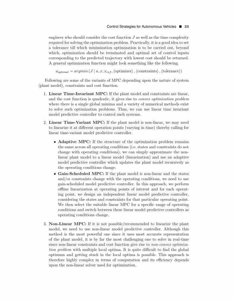
engineer who should consider the cost function J as well as the time complexityrequired for solving the optimization problem. Practically, it is a good idea to seta tolerance till which minimization optimization is to be carried out, beyondwhich, optimization should be terminated and optimal set of control inputscorresponding to the predicted trajectory with lowest cost should be returned.A general optimization function might look something like the following.
uoptimal = argmin (J | u, x, xref , 〈optimizer〉 , 〈constraints〉 , 〈tolerance〉)
Following are some of the variants of MPC depending upon the nature of system(plant model), constraints and cost function.
1. Linear Time-Invariant MPC: If the plant model and constraints are linear,and the cost function is quadratic, it gives rise to convex optimization problemwhere there is a single global minima and a variety of numerical methods existto solve such optimization problems. Thus, we can use linear time invariantmodel predictive controller to control such systems.
2. Linear Time-Variant MPC: If the plant model is non-linear, we may needto linearize it at different operation points (varying in time) thereby calling forlinear time-variant model predictive controller.
• Adaptive MPC: If the structure of the optimization problem remainsthe same across all operating conditions (i.e. states and constraints do notchange with operating conditions), we can simply approximate the non-linear plant model to a linear model (linearization) and use an adaptivemodel predictive controller which updates the plant model recursively asthe operating conditions change.• Gain-Scheduled MPC: If the plant model is non-linear and the states
and/or constraints change with the operating conditions, we need to usegain-scheduled model predictive controller. In this approach, we performoffline linearization at operating points of interest and for each operat-ing point, we design an independent linear model predictive controller,considering the states and constraints for that particular operating point.We then select the suitable linear MPC for a specific range of operatingconditions and switch between these linear model predictive controllers asoperating conditions change.
3. Non-Linear MPC: If it is not possible/recommended to linearize the plantmodel, we need to use non-linear model predictive controller. Although thismethod is the most powerful one since it uses most accurate representationof the plant model, it is by far the most challenging one to solve in real-timesince non-linear constraints and cost function give rise to non-convex optimiza-tion problem with multiple local optima. It is quite difficult to find the globaloptimum and getting stuck in the local optima is possible. This approach istherefore highly complex in terms of computation and its efficiency dependsupon the non-linear solver used for optimization.
34 � Control Strategies for Autonomous Vehicles
A general rule of thumb for selecting from the variants of MPC is to start simpleand go complex if and only if it is necessary. Thus, linear time-invariant or traditionalMPC and adaptive MPC are the two most commonly used approaches for autonomousvehicle control under nominal driving conditions.
Model Predictive Control Implementation
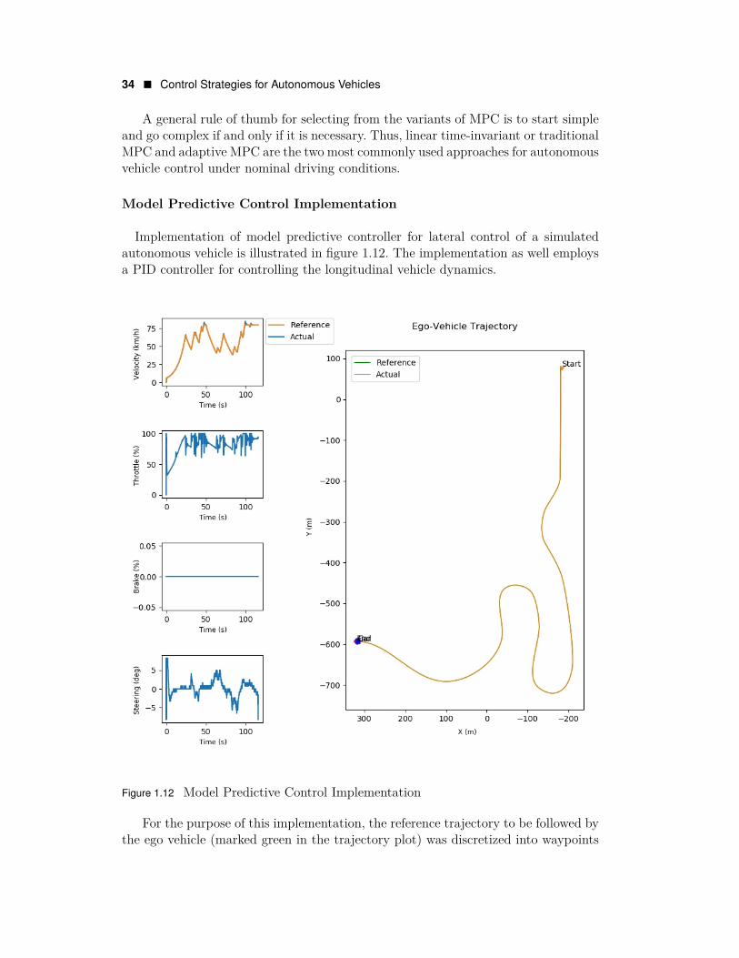
Implementation of model predictive controller for lateral control of a simulatedautonomous vehicle is illustrated in figure 1.12. The implementation as well employsa PID controller for controlling the longitudinal vehicle dynamics.
Figure 1.12 Model Predictive Control Implementation
For the purpose of this implementation, the reference trajectory to be followed bythe ego vehicle (marked green in the trajectory plot) was discretized into waypoints
Control Strategies for Autonomous Vehicles � 35
to be tracked by the lateral controller, and each waypoint had an associated velocitysetpoint to be tracked by the longitudinal controller.
A simple kinematic bicycle model also worked really well for tracking the entirereference trajectory (which included both straight as well as curved segments) atvarying longitudinal velocities. The model predictive controller was able to track theprescribed trajectory with a promising level of precision and accuracy. Additionally,the steering control commands generated during the entire course of simulation liedwell within the span δ ∈ [−10◦, 10◦], which is an indication of the controller beingable to generate optimal control actions at right time instants.
One of the most significant drawback of MPC is its heavy requirement of compu-tational resources. However, this can be easily counteracted by limiting the predictionand control horizons to moderately-small and small magnitudes, formulating simplercost functions, using less detailed motion models or setting a higher tolerance for op-timization convergence. Although this may lead to sub-optimal solutions, it reducescomputational overhead to a great extent, thereby ensuring real-time execution ofthe control algorithm.
In conclusion, model predictive control can be regarded as the best control strat-egy for both simplistic as well as rigorous driving behaviors, provided a sufficientlypowerful computational resource is available online.
1.3.3 Learning Based Control
As stated in section 1.3.2, traditional controllers require in-depth knowledge of theprocess flow involved in designing and tuning them. Additionally, in case of modelbased controllers, the physical parameters of the system, along with its kinematicand/or dynamic models need to be known before designing a suitable controller. Toadd to the problem, most traditional controllers are scenario-specific and do not adaptto varying operating conditions; they need to be re-tuned in case of a scenario-change,which makes them quite inconvenient to work with. Lastly, most of the advanced tra-ditional controllers are computationally expensive, which induces a time lag derivederror in the processing pipeline.
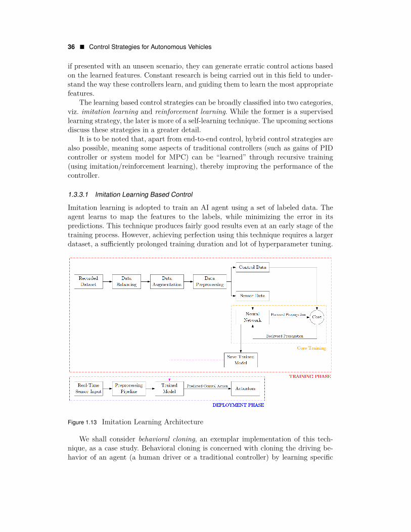
Recently, learning based control strategies have started blooming, especially end-to-end learning. Such controllers hardly require any system-level knowledge and aremuch easier to implement. The system engineer may not need to implement the per-ception, planning and control sub-systems, since the AI agent learns to perform theseoperations implicitly; it is rather difficult to exactly tell which part of the neural net-work acts as the perception sub-system, which acts as planning sub-system and whichacts as the control sub-system. Although the “learning” process is computationallyquite expensive, this step may be performed offline for a single time, after which, thetrained model may be incorporated into the system architecture of the autonomousvehicle for a real-time implementation. Another advantage of such controllers is theirability to generalize across a range of similar scenarios, which makes them fit forminor deviations in the driving conditions. All in all, learning based control schemesseem to be a tempting alternative for the traditional ones. However, there is still along way in achieving this goal as learning based controllers are somewhat unreliable;
36 � Control Strategies for Autonomous Vehicles
if presented with an unseen scenario, they can generate erratic control actions basedon the learned features. Constant research is being carried out in this field to under-stand the way these controllers learn, and guiding them to learn the most appropriatefeatures.
The learning based control strategies can be broadly classified into two categories,viz. imitation learning and reinforcement learning. While the former is a supervisedlearning strategy, the later is more of a self-learning technique. The upcoming sectionsdiscuss these strategies in a greater detail.
It is to be noted that, apart from end-to-end control, hybrid control strategies arealso possible, meaning some aspects of traditional controllers (such as gains of PIDcontroller or system model for MPC) can be “learned” through recursive training(using imitation/reinforcement learning), thereby improving the performance of thecontroller.
1.3.3.1 Imitation Learning Based Control
Imitation learning is adopted to train an AI agent using a set of labeled data. Theagent learns to map the features to the labels, while minimizing the error in itspredictions. This technique produces fairly good results even at an early stage of thetraining process. However, achieving perfection using this technique requires a largerdataset, a sufficiently prolonged training duration and lot of hyperparameter tuning.
Figure 1.13 Imitation Learning Architecture
We shall consider behavioral cloning, an exemplar implementation of this tech-nique, as a case study. Behavioral cloning is concerned with cloning the driving be-havior of an agent (a human driver or a traditional controller) by learning specific
Control Strategies for Autonomous Vehicles � 37
features from the training dataset provided. Figure 1.13 illustrates the training anddeployment phases of imitation learning, which are discussed in the following sections.
Training Phase
During the training phase, the ego vehicle is driven (either manually or using atraditional controller) in a scenario resembling one in the deployment phase, andtimestamped sensor readings (images, point cloud, etc.) along with the control in-put measurements (throttle, brake and steering) are recorded in a driving log. Thecollected dataset is then balanced to remove any inherent prejudice after which, it isaugmented and preprocessed, thereby imparting robustness to the model and helpingit generalize to a range of similar scenarios. Practically, the augmentation and pre-processing steps are performed on-the-go during the training process using a batchgenerator. Finally, a deep neural network is “trained” to directly predict the controlinputs based on sensor readings.
It is to be noted that, practically, the collected dataset influences the trainingprocess more than anything else. Other important factors affecting the training, inorder of importance, include neural network architecture (coarse-tuning is sufficientin most cases), augmentation and preprocessing techniques used and hyperparame-ter values chosen (fine-tuning may be required based on the application). It is alsocompletely possible that one training pipeline works well on one dataset, while theother works well on a different one.
Training a neural network end-to-end in order to predict the control actions re-quired to drive an autonomous vehicle based on the sensory inputs is essentiallymodeling the entire system as a linear combination of input features to predict theoutput labels. The training process can be elucidated as follows.
First a suitable neural network architecture is defined; this architecture may beiteratively modified based on experimental results. The trainable parameters of themodel include weights and biases. Generally, the weights are initialized to a smallnon-zero random value, whereas the biases are initialized to zero.
The network then performs, what is called, a forward propagation step. Here,each neuron of every layer of the neural network calculates a weighted average ofthe activated input vector a it receives from the previous layer, based on its currentweight vector wi and adds a bias term bi to it. For the first layer, however, the inputvector x is considered in place of a[l−1]. The result of this operation zi is then passedthrough a non-linear activation function g(z), to produce an activated output ai.
z[l]i = wTi · a[l−1] + bi
a[l]i = g[l](z[l]
i )
Note that l here, denotes the lth layer of the neural network and i denotes the ithneuron of that layer.
Practically, however, these operations are not performed sequentially for each
38 � Control Strategies for Autonomous Vehicles
and every neuron. Instead, vectorization is adopted, which groups the similar vari-ables and vectors into distinct matrices and performs all the matrix manipulations atonce, thereby reducing the computational complexity of the operation. The activatedoutput vector of last layer is termed as predicted output y of the neural network.
The predicted output y is then used to compute the loss L of the forward prop-agation, based on the loss function defined. Intuitively, loss is basically a measure ofincorrectness (i.e. error) of the predicted output w.r.t. the labeled output.
Generally, for a regression problem like the one we are talking about, the mostcommonly adopted loss function is the mean squared error (MSE). It is defined asfollows.
L(y, y) = 1n
n∑i=1‖yi − yi‖2
For classification problems, though, the cross-entropy loss function is a favorablechoice. For a dataset with M different classes, it is defined as follows.
L(y, y) ={−(yi ∗ log(yi) + (1− yi) ∗ log(1− yi)) ;M = 2−∑Mi=1 yi ∗ log(yi) ;M > 2
The equations defined above are used to compute loss for each training example.These individual losses L over m training examples can be used to evaluate an overallcost J using the following relation.
J(w, b) = 1m
m∑i=1
L( ˆy(i), y(i))
Note that w and b in the above equation denote vectorized form of weights andbiases respectively, across the entire training set (or a mini-batch).
The cost is then minimized by recursively updating the weights and biases usingan optimizer. This step is known as back propagation.
The most traditional optimizer is the gradient decent algorithm. In its very rudi-mentary form, the algorithm updates trainable parameters (i.e. weights and biases)by subtracting from them their respective gradients dw and db w.r.t. the cost functionJ , scaled by the learning rate hyperparameter α.{
w[l] = w[l] − α ∗ dw[l]
b[l] = b[l] − α ∗ db[l]
Where, dw and db are computed as follows.{dw[l] = ∂J
∂w[l] = dz[l] · a[l−1]
db[l] = ∂J∂b[l] = dz[l]
Here, dz and da, interdependent on each other, can be computed using the fol-lowing relations.
Control Strategies for Autonomous Vehicles � 39
{dz[l] = da[l] ∗ g[l]′(z[l])da[l−1] = w[l]T · dz[l]
However, the current state-of-the-art optimizer adopted by most domain expertsis the Adam optimizer. The algorithm commences by computing the gradients dwand db using the gradient descent method and then computes the exponential movingaverages of the gradients V and their squares S, similar to Momentum and RMSpropalgorithms respectively. {
Vdw = β1 ∗ Vdw + (1− β1) ∗ dwVdb = β1 ∗ Vdb + (1− β1) ∗ db{Sdw = β2 ∗ Sdw + (1− β2) ∗ dw2
Sdb = β2 ∗ Sdb + (1− β2) ∗ db2
The bias correction equations for the exponential moving averages after t itera-tions are given as follows. Vdw = Vdw
(1−βt1)
Vdb = Vdb(1−βt1)Sdw = Sdw(1−βt2)
Sdb = Sdb(1−βt2)
The final update equations for the training parameters are therefore as givenbelow.
w = w − α ∗ Vdw√Sdw+ε
b = b− α ∗ Vdb√Sdb+ε
Note that ε in the above equations is a small factor that prevents division byzero. The authors of Adam optimizer propose the default values of 0.9 for β1, 0.999for β2 and 10−8 for ε.They show empirically that Adam works well in practice andcompares favorably to other adaptive learning based algorithms.
Deployment Phase
During the deployment phase, the trained model is incorporated into the controlarchitecture of the ego vehicle to predict (forward propagation step alone) the sameset of control inputs (throttle, brake and steering) based on measurements (images,point cloud, etc.) from the same set of sensors as during the training phase, in realtime.
It is worth mentioning that the pipeline adopted for the deployment phase shouldhave minimum latency in order to ensure real-time performance.
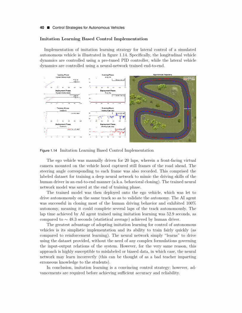
40 � Control Strategies for Autonomous Vehicles
Imitation Learning Based Control Implementation
Implementation of imitation learning strategy for lateral control of a simulatedautonomous vehicle is illustrated in figure 1.14. Specifically, the longitudinal vehicledynamics are controlled using a pre-tuned PID controller, while the lateral vehicledynamics are controlled using a neural-network trained end-to-end.
Figure 1.14 Imitation Learning Based Control Implementation
The ego vehicle was manually driven for 20 laps, wherein a front-facing virtualcamera mounted on the vehicle hood captured still frames of the road ahead. Thesteering angle corresponding to each frame was also recorded. This comprised thelabeled dataset for training a deep neural network to mimic the driving skills of thehuman driver in an end-to-end manner (a.k.a. behavioral cloning). The trained neuralnetwork model was saved at the end of training phase.
The trained model was then deployed onto the ego vehicle, which was let todrive autonomously on the same track so as to validate the autonomy. The AI agentwas successful in cloning most of the human driving behavior and exhibited 100%autonomy, meaning it could complete several laps of the track autonomously. Thelap time achieved by AI agent trained using imitation learning was 52.9 seconds, ascompared to ∼ 48.3 seconds (statistical average) achieved by human driver.
The greatest advantage of adopting imitation learning for control of autonomousvehicles is its simplistic implementation and its ability to train fairly quickly (ascompared to reinforcement learning). The neural network simply “learns” to driveusing the dataset provided, without the need of any complex formulations governingthe input-output relations of the system. However, for the very same reason, thisapproach is highly susceptible to mislabeled or biased data, in which case, the neuralnetwork may learn incorrectly (this can be thought of as a bad teacher impartingerroneous knowledge to the students).
In conclusion, imitation learning is a convincing control strategy; however, ad-vancements are required before achieving sufficient accuracy and reliability.
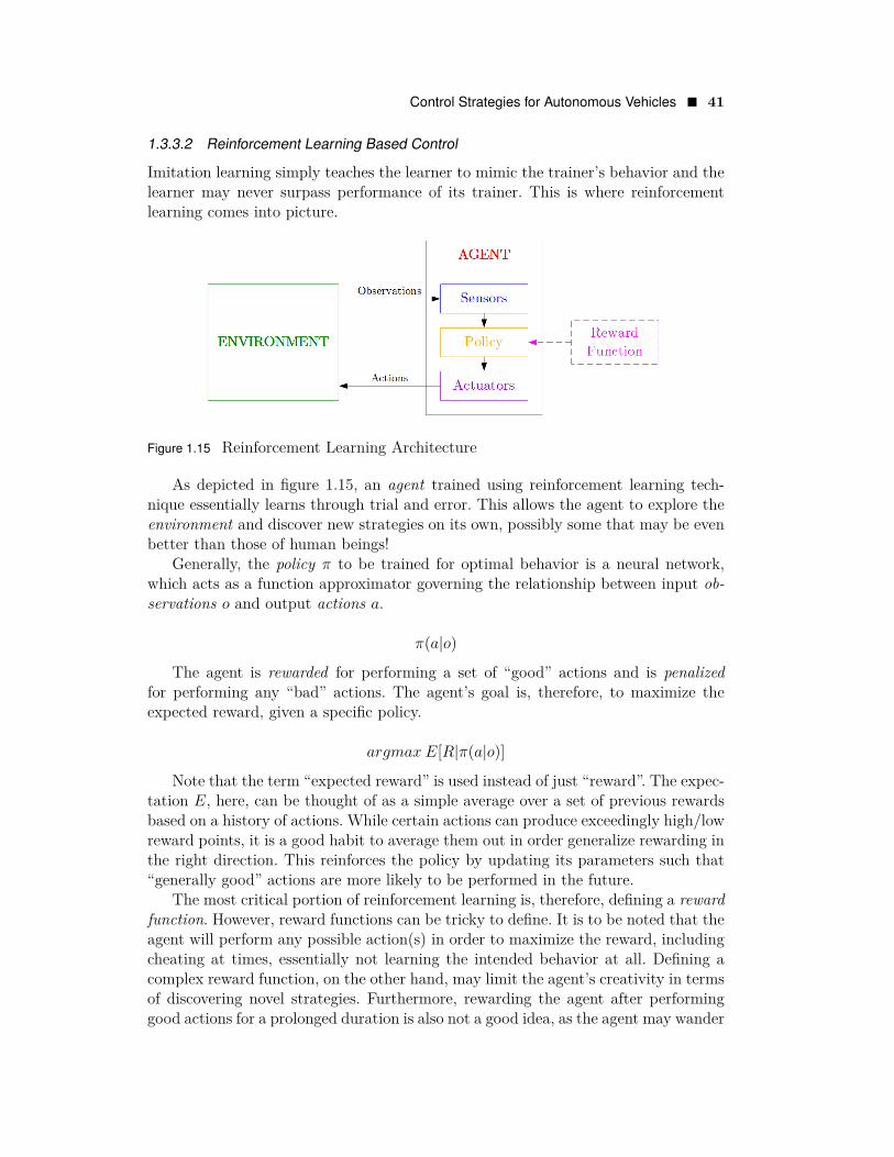
Control Strategies for Autonomous Vehicles � 41
1.3.3.2 Reinforcement Learning Based Control
Imitation learning simply teaches the learner to mimic the trainer’s behavior and thelearner may never surpass performance of its trainer. This is where reinforcementlearning comes into picture.
Figure 1.15 Reinforcement Learning Architecture
As depicted in figure 1.15, an agent trained using reinforcement learning tech-nique essentially learns through trial and error. This allows the agent to explore theenvironment and discover new strategies on its own, possibly some that may be evenbetter than those of human beings!
Generally, the policy π to be trained for optimal behavior is a neural network,which acts as a function approximator governing the relationship between input ob-servations o and output actions a.
π(a|o)
The agent is rewarded for performing a set of “good” actions and is penalizedfor performing any “bad” actions. The agent’s goal is, therefore, to maximize theexpected reward, given a specific policy.
argmax E[R|π(a|o)]
Note that the term “expected reward” is used instead of just “reward”. The expec-tation E, here, can be thought of as a simple average over a set of previous rewardsbased on a history of actions. While certain actions can produce exceedingly high/lowreward points, it is a good habit to average them out in order generalize rewarding inthe right direction. This reinforces the policy by updating its parameters such that“generally good” actions are more likely to be performed in the future.
The most critical portion of reinforcement learning is, therefore, defining a rewardfunction. However, reward functions can be tricky to define. It is to be noted that theagent will perform any possible action(s) in order to maximize the reward, includingcheating at times, essentially not learning the intended behavior at all. Defining acomplex reward function, on the other hand, may limit the agent’s creativity in termsof discovering novel strategies. Furthermore, rewarding the agent after performinggood actions for a prolonged duration is also not a good idea, as the agent may wander
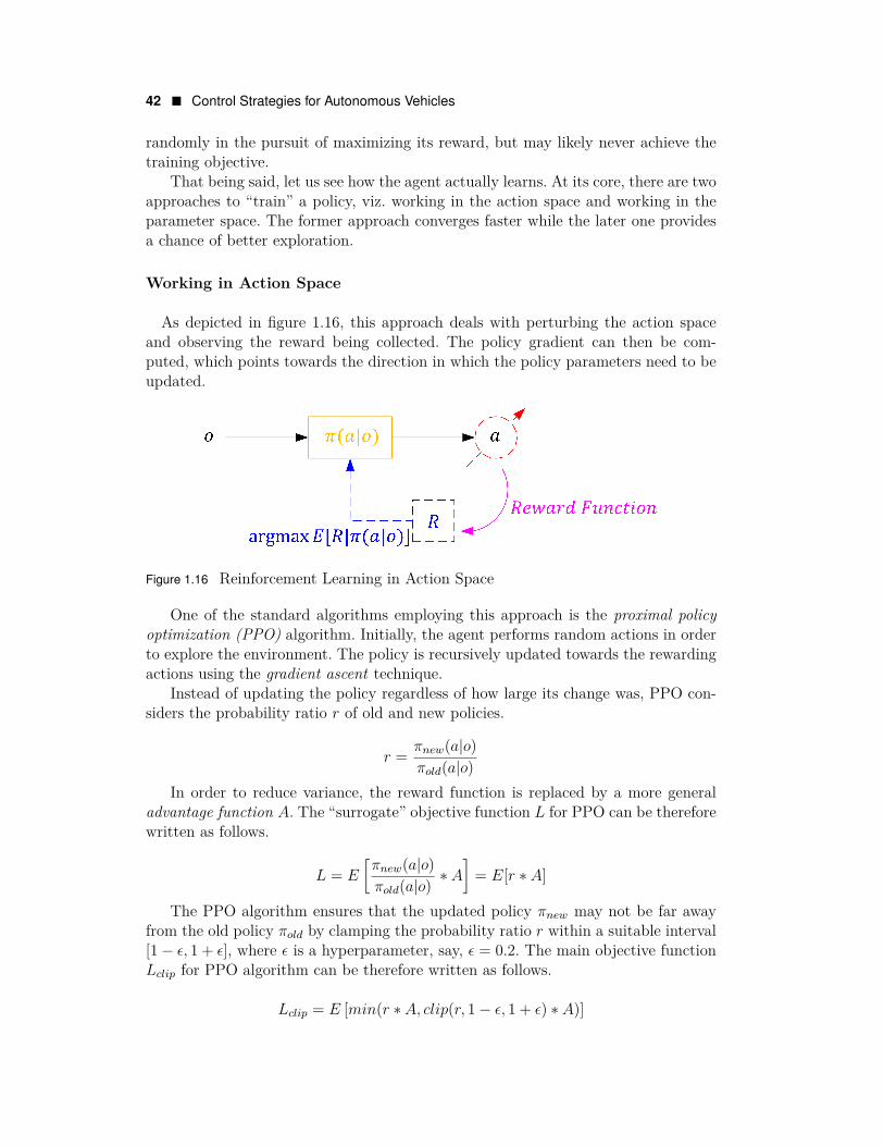
42 � Control Strategies for Autonomous Vehicles
randomly in the pursuit of maximizing its reward, but may likely never achieve thetraining objective.
That being said, let us see how the agent actually learns. At its core, there are twoapproaches to “train” a policy, viz. working in the action space and working in theparameter space. The former approach converges faster while the later one providesa chance of better exploration.
Working in Action Space
As depicted in figure 1.16, this approach deals with perturbing the action spaceand observing the reward being collected. The policy gradient can then be com-puted, which points towards the direction in which the policy parameters need to beupdated.
Figure 1.16 Reinforcement Learning in Action Space
One of the standard algorithms employing this approach is the proximal policyoptimization (PPO) algorithm. Initially, the agent performs random actions in orderto explore the environment. The policy is recursively updated towards the rewardingactions using the gradient ascent technique.
Instead of updating the policy regardless of how large its change was, PPO con-siders the probability ratio r of old and new policies.
r = πnew(a|o)πold(a|o)
In order to reduce variance, the reward function is replaced by a more generaladvantage function A. The “surrogate” objective function L for PPO can be thereforewritten as follows.
L = E
[πnew(a|o)πold(a|o)
∗ A]
= E[r ∗ A]
The PPO algorithm ensures that the updated policy πnew may not be far awayfrom the old policy πold by clamping the probability ratio r within a suitable interval[1− ε, 1 + ε], where ε is a hyperparameter, say, ε = 0.2. The main objective functionLclip for PPO algorithm can be therefore written as follows.
Lclip = E [min(r ∗ A, clip(r, 1− ε, 1 + ε) ∗ A)]
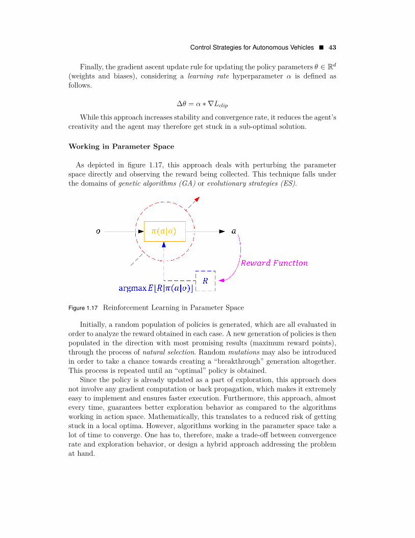
Control Strategies for Autonomous Vehicles � 43
Finally, the gradient ascent update rule for updating the policy parameters θ ∈ Rd(weights and biases), considering a learning rate hyperparameter α is defined asfollows.
∆θ = α ∗ ∇LclipWhile this approach increases stability and convergence rate, it reduces the agent’s
creativity and the agent may therefore get stuck in a sub-optimal solution.
Working in Parameter Space
As depicted in figure 1.17, this approach deals with perturbing the parameterspace directly and observing the reward being collected. This technique falls underthe domains of genetic algorithms (GA) or evolutionary strategies (ES).
Figure 1.17 Reinforcement Learning in Parameter Space
Initially, a random population of policies is generated, which are all evaluated inorder to analyze the reward obtained in each case. A new generation of policies is thenpopulated in the direction with most promising results (maximum reward points),through the process of natural selection. Random mutations may also be introducedin order to take a chance towards creating a “breakthrough” generation altogether.This process is repeated until an “optimal” policy is obtained.
Since the policy is already updated as a part of exploration, this approach doesnot involve any gradient computation or back propagation, which makes it extremelyeasy to implement and ensures faster execution. Furthermore, this approach, almostevery time, guarantees better exploration behavior as compared to the algorithmsworking in action space. Mathematically, this translates to a reduced risk of gettingstuck in a local optima. However, algorithms working in the parameter space take alot of time to converge. One has to, therefore, make a trade-off between convergencerate and exploration behavior, or design a hybrid approach addressing the problemat hand.
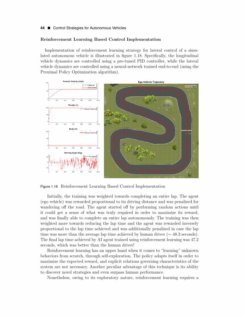
44 � Control Strategies for Autonomous Vehicles
Reinforcement Learning Based Control Implementation
Implementation of reinforcement learning strategy for lateral control of a simu-lated autonomous vehicle is illustrated in figure 1.18. Specifically, the longitudinalvehicle dynamics are controlled using a pre-tuned PID controller, while the lateralvehicle dynamics are controlled using a neural-network trained end-to-end (using theProximal Policy Optimization algorithm).
Figure 1.18 Reinforcement Learning Based Control Implementation
Initially, the training was weighted towards completing an entire lap. The agent(ego vehicle) was rewarded proportional to its driving distance and was penalized forwandering off the road. The agent started off by performing random actions untilit could get a sense of what was truly required in order to maximize its reward,and was finally able to complete an entire lap autonomously. The training was thenweighted more towards reducing the lap time and the agent was rewarded inverselyproportional to the lap time achieved and was additionally penalized in case the laptime was more than the average lap time achieved by human driver (∼ 48.3 seconds).The final lap time achieved by AI agent trained using reinforcement learning was 47.2seconds, which was better than the human driver!
Reinforcement learning has an upper hand when it comes to “learning” unknownbehaviors from scratch, through self-exploration. The policy adapts itself in order tomaximize the expected reward, and explicit relations governing characteristics of thesystem are not necessary. Another peculiar advantage of this technique is its abilityto discover novel strategies and even surpass human performance.
Nonetheless, owing to its exploratory nature, reinforcement learning requires a
Control Strategies for Autonomous Vehicles � 45
significantly high amount of training time, which might pose as a major issue incase of development-analysis cycles. Furthermore, this approach calls for a hand-crafted reward function, which, if defined inefficiently, may cause unintended reward-ing, thereby leading to erroneous learning.
In conclusion, reinforcement learning is a powerful strategy, especially in terms ofachieving super-human performance. However, it is generally better to have at leasta basic pre-trained model available to work on top of, in order to skip the initial (andmost time consuming) portion of the training phase, wherein the agent generatesalmost random actions with an aim of primary exploration.
1.4 OUR RESEARCH AT AUTONOMOUS SYSTEMS LAB (SRMIST)
Autonomous Systems Lab at the Department of Mechatronics Engineering, SRMInstitute of Science and Technology (SRMIST) is headed by Mr. K. Sivanathan, andis focused on research and development in various aspects of autonomous systems.Specifically focusing on autonomous vehicles, our team is constantly working on allthe three sub-systems viz. perception, planning and control. Although most of ourpast works are limited to simulation, we are currently working towards developingour own research platform for testing hardware implementations as well.
Further narrowing down to control of autonomous vehicles, our team has workedon most of the aforementioned control strategies, if not all, and we are continuouslystudying and experimenting with them in order to analyze their performance andtest their limits. We are also working on developing novel and hybrid control strate-gies with an aim of ameliorating the controller performance (i.e. improved stability,tracking and robustness) and/or reducing computational cost (allowing real-time ex-ecution).
It is to be noted that an exhaustive discussion on each and every research projectcarried out at Autonomous Systems Lab (SRMIST) is beyond the scope of this chap-ter. Nonetheless, some of our team’s research project demonstrations pertaining toautonomous vehicles are available at:www.youtube.com/playlist?list=PLdOCgvQ2Iny8g9OPmEJeVCas9tKr6auB3
1.5 CLOSING REMARKS
Throughout this chapter, we have discussed most of the current state-of-the-art con-trol strategies employed for autonomous vehicles, right from the basic ones such asbang-bang and PID control all the way up to advanced ones such as MPC and end-to-end learning, from theoretical, conceptual as well as practical viewpoints. Now,as we come towards the end of this chapter, we would like to add a few notes onsome minute details pertaining to performance enhancement of control strategies forautonomous vehicles based on our knowledge and experience in the field.
• Gain Scheduling: Most non-linear systems exhibit varying dynamics underdifferent operating conditions. In such cases, a controller with single set ofgains may not be able to regulate the system effectively throughout the opera-tional design domain as the operating conditions change. The gain scheduling
46 � Control Strategies for Autonomous Vehicles
technique overcomes this limitation by employing multiple sets of gains appro-priately across the entire range of operating conditions.
• Integral Windup: For PI and PID controllers, integrating the error over aprolonged duration may lead to very large values, resulting in loss of stability. Itis, therefore, advised to limit the upper value of the accumulated error to a safevalue. This can be achieved using a wide array of techniques, one of them beingimposition of upper and lower bounds on the accumulated error and clippingthe value within that range. Another approach would be limiting the size ofhistory buffer over which the error is integrated through the use of a queuedata structure of limited size based on the first-in-first-out (FIFO) principle todiscard error values that are too old.
• Smoothing Controller Outputs: Most of the controllers have a tendencyof generating abrupt responses in case of a highly dynamic event, and whileit may be appropriate in a few cases, it is generally undesirable. Such abruptcontrol actions may cause loss of stability or even affect the actuation elementsadversely. It, therefore, becomes necessary to sooth the controller outputs beforeapplying them to the plant, and one way of achieving this is to clamp thecontroller outputs within a safe range (determined through rigorous testing),such that the controller is still able to track the setpoint under all the operatingconditions. A secondary approach would comprise of limiting the rate of changeof the control output, thereby enabling a smoother transition.
• Introduction of Dead-Bands: Most corrective controllers oscillate about thesetpoint, trying really hard to converge, and while this might be desirable incase of highly precise systems, it is generally not really necessary to achieve thesetpoint exactly. The controller action may be nullified within close neighbor-hood of the setpoint. This is known as a dead-band. It must be noted, however,that the width of the dead-band must be chosen wisely, depending upon theprecision requirements of the system in question.
• Safe Reinforcement Learning: As discussed earlier, reinforcement learn-ing involves discovery of novel strategies majorly through a trial-and-errorapproach, due to which, it is seldom directly applied to a physical system(you don’t want to take millions of episodes to learn by crashing the agentalmost each time). However, there are a few techniques that can be employedto overcome this limitation, one of them being training a simulated agent underpseudo-realistic operating conditions and then transferring the trained modelonto the physical agent. Another way of approaching this problem would beto penalize the policy prior to any catastrophic event by self-supervising theagent through an array of sensors. A third (and more elegant) approach wouldbe to train the agent for a “safe” behavior using imitation learning and thenimproving its performance by training it further using reinforcement learning.
As a final note, we summarize the control strategies described in this chapteragainst a set of qualitative comparison metrics in table 1.2.
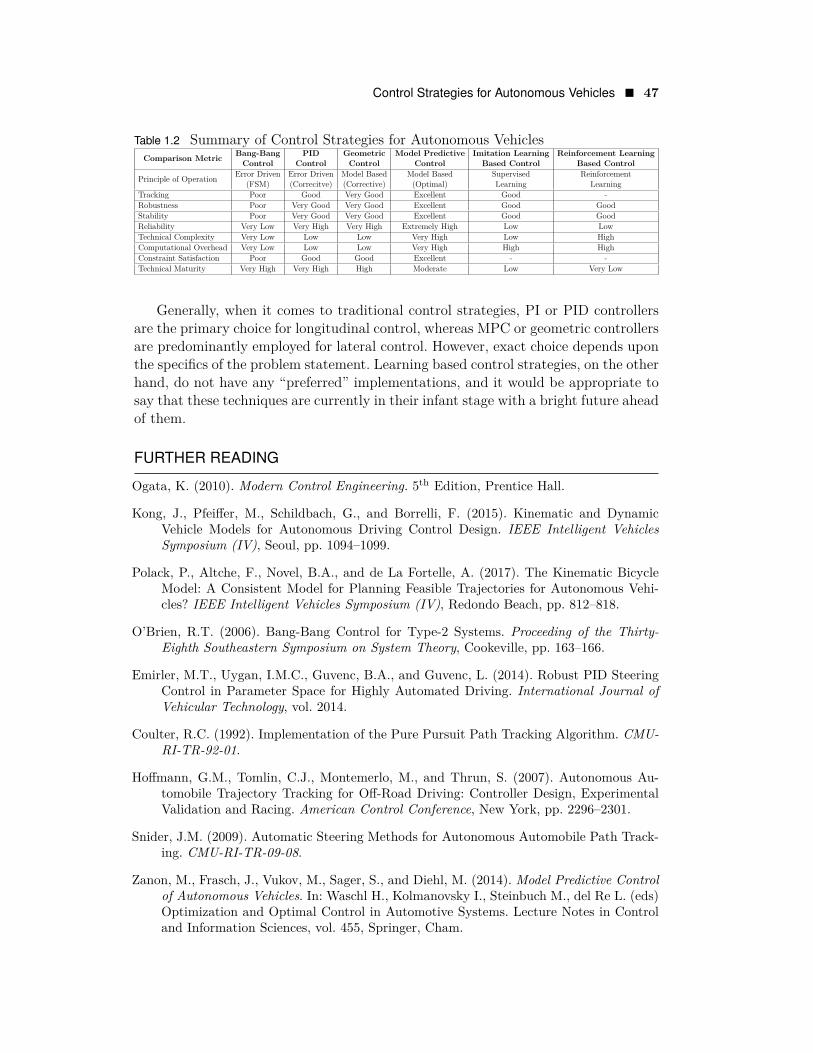
Control Strategies for Autonomous Vehicles � 47
Table 1.2 Summary of Control Strategies for Autonomous VehiclesComparison Metric Bang-Bang
ControlPID
ControlGeometric
ControlModel Predictive
ControlImitation Learning
Based ControlReinforcement Learning
Based Control
Principle of Operation Error Driven(FSM)
Error Driven(Correcitve)
Model Based(Corrective)
Model Based(Optimal)
SupervisedLearning
ReinforcementLearning
Tracking Poor Good Very Good Excellent Good -Robustness Poor Very Good Very Good Excellent Good GoodStability Poor Very Good Very Good Excellent Good GoodReliability Very Low Very High Very High Extremely High Low LowTechnical Complexity Very Low Low Low Very High Low HighComputational Overhead Very Low Low Low Very High High HighConstraint Satisfaction Poor Good Good Excellent - -Technical Maturity Very High Very High High Moderate Low Very Low
Generally, when it comes to traditional control strategies, PI or PID controllersare the primary choice for longitudinal control, whereas MPC or geometric controllersare predominantly employed for lateral control. However, exact choice depends uponthe specifics of the problem statement. Learning based control strategies, on the otherhand, do not have any “preferred” implementations, and it would be appropriate tosay that these techniques are currently in their infant stage with a bright future aheadof them.
FURTHER READING
Ogata, K. (2010). Modern Control Engineering. 5th Edition, Prentice Hall.
Kong, J., Pfeiffer, M., Schildbach, G., and Borrelli, F. (2015). Kinematic and DynamicVehicle Models for Autonomous Driving Control Design. IEEE Intelligent VehiclesSymposium (IV), Seoul, pp. 1094–1099.
Polack, P., Altche, F., Novel, B.A., and de La Fortelle, A. (2017). The Kinematic BicycleModel: A Consistent Model for Planning Feasible Trajectories for Autonomous Vehi-cles? IEEE Intelligent Vehicles Symposium (IV), Redondo Beach, pp. 812–818.
O’Brien, R.T. (2006). Bang-Bang Control for Type-2 Systems. Proceeding of the Thirty-Eighth Southeastern Symposium on System Theory, Cookeville, pp. 163–166.
Emirler, M.T., Uygan, I.M.C., Guvenc, B.A., and Guvenc, L. (2014). Robust PID SteeringControl in Parameter Space for Highly Automated Driving. International Journal ofVehicular Technology, vol. 2014.
Coulter, R.C. (1992). Implementation of the Pure Pursuit Path Tracking Algorithm. CMU-RI-TR-92-01.
Hoffmann, G.M., Tomlin, C.J., Montemerlo, M., and Thrun, S. (2007). Autonomous Au-tomobile Trajectory Tracking for Off-Road Driving: Controller Design, ExperimentalValidation and Racing. American Control Conference, New York, pp. 2296–2301.
Snider, J.M. (2009). Automatic Steering Methods for Autonomous Automobile Path Track-ing. CMU-RI-TR-09-08.
Zanon, M., Frasch, J., Vukov, M., Sager, S., and Diehl, M. (2014). Model Predictive Controlof Autonomous Vehicles. In: Waschl H., Kolmanovsky I., Steinbuch M., del Re L. (eds)Optimization and Optimal Control in Automotive Systems. Lecture Notes in Controland Information Sciences, vol. 455, Springer, Cham.
48 � Control Strategies for Autonomous Vehicles
Babu, M., Theerthala, R.R., Singh, A.K., Baladhurgesh B.P., Gopalakrishnan, B., and Kr-ishna, K.M. (2019). Model Predictive Control for Autonomous Driving considering Ac-tuator Dynamics. American Control Conference (ACC), Philadelphia, pp. 1983–1989.
Obayashi, M., and Takano, G. (2018). Real-Time Autonomous Car Motion Planning usingNMPC with Approximated Problem Considering Traffic Environment. 6th IFAC Con-ference on Nonlinear Model Predictive Control NMPC, IFAC-PapersOnLine, vol. 51,no. 20, pp. 279–286.
Tampuu, A., Semikin, M., Muhammad, N., Fishman, D., and Matiisen, T. (2020).A Survey of End-to-End Driving: Architectures and Training Methods. Preprint,arXiv:2003.06404.
Pomerleau, D. (1989). ALVINN: An Autonomous Land Vehicle In a Neural Network. Pro-ceedings of Advances in Neural Information Processing Systems 1, pp. 305–313.
LeCun, Y., Muller, U., Ben, J., Cosatto, E., and Flepp, B. (2005). Off-Road Obstacle Avoid-ance through End-to-End Learning. Advances in Neural Information Processing Sys-tems, pp. 739–746.
Bojarski, M., Testa, D.D., Dworakowski, D., Firner, B., Flepp, B., Goyal, P., Jackel, L.D.,Monfort, M., Muller, U., Zhang, J., Zhang, X., Zhao, J., and Zieba, K. (2016). End toEnd Learning for Self-Driving Cars. Preprint, arXiv:1604.07316.
Samak, T.V., Samak, C.V., and Kandhasamy, S. (2020). Robust Behavioral Cloning for Au-tonomous Vehicles using End-to-End Imitation Learning. Preprint, arXiv:2010.04767.
Li, D., Zhao, D., Zhang, Q., and Chen, Y. (2019). Reinforcement Learning and Deep Learn-ing Based Lateral Control for Autonomous Driving [Application Notes]. IEEE Com-putational Intelligence Magazine, vol. 14, no. 2, pp. 83–98.
Riedmiller, M., Montemerlo, M., and Dahlkamp, H. (2007). Learning to Drive a Real Car in20 Minutes. Frontiers in the Convergence of Bioscience and Information Technologies,Jeju City, pp. 645–650.
Kendall, A., Hawke, J., Janz, D., Mazur, P., Reda, D., Allen, J.M., Lam, V.D., Bewley, A.,and Shah, A. (2018). Learning to Drive in a Day. Preprint, arXiv:1807.00412.
Kabzan, J., Hewing, L., Liniger, A., and Zeilinger, M.N. (2019). Learning-Based ModelPredictive Control for Autonomous Racing. IEEE Robotics and Automation Letters,vol. 4, no. 4, pp. 3363–3370.
Rosolia, U., and Borrelli, F. (2020). Learning How to Autonomously Race a Car: A PredictiveControl Approach. IEEE Transactions on Control Systems Technology, vol. 28, no. 6,pp. 2713–2719.
Drews, P., Williams, G., Goldfain, B., Theodorou, E.A., and Rehg, J.M. (2018). Vision-BasedHigh Speed Driving with a Deep Dynamic Observer. Preprint, arXiv:1812.02071.


![Autonomous vehicles[1]](https://img.pdfslide.us/doc/110x75/54bf07bb4a7959cb478b4592/autonomous-vehicles1.jpg)