Embed Size (px)
Citation preview

Purdue UniversityPurdue e-Pubs
Open Access Dissertations Theses and Dissertations
Spring 2015
Control oriented concentrating solar power (CSP)plant model and its applicationsQi LuoPurdue University
Follow this and additional works at: https://docs.lib.purdue.edu/open_access_dissertations
Part of the Mechanical Engineering Commons
This document has been made available through Purdue e-Pubs, a service of the Purdue University Libraries. Please contact [email protected] foradditional information.
Recommended CitationLuo, Qi, "Control oriented concentrating solar power (CSP) plant model and its applications" (2015). Open Access Dissertations. 509.https://docs.lib.purdue.edu/open_access_dissertations/509

! ! " # ! ! $ %& ! ' ! # % ( ! ! ' ! " # ! ' ! ) * + ' , - . / % ! ! " ! ! 0 1 ! ! & 2 ! 1 ! 3 4 & ! ' 5 ! ! 6 ' 7 ' 0 ! ! 8
9 : ; < => ? @ A B ? C ? B D E @ A E F > ? @ > E @ A B G A D @ H I ? C G B J ? K E B L > I J M J C G @ AN ? F E C G @ F D A I G J J C D > G A D ? @ IO = P Q = R = S T U : V = W = X U YZ [ \ ] ^ _ G \ ^ ` a \I a \ b c d H [ \ ^ e b f f [I a g [ ] h > d [ _ \ [ i [ \ ] `G ] d a f [ Z a f [ ] a j g [
Z [ \ ] ^ _ G \ ^ ` a \G j ^ f k [ l [ l m n o p q o n m p r

CONTROL ORIENTED CONCENTRATING SOLAR POWER (CSP) PLANT
MODEL AND ITS APPLICATIONS
A Dissertation
Submitted to the Faculty
of
Purdue University
by
Qi Luo
In Partial Fulfillment of the
Requirements for the Degree
of
Doctor of Philosophy
May 2015
Purdue University
West Lafayette, Indiana

ii
I dedicate my dissertation work to my family. A special gratitude to my loving
parents, Piduo Luo and Guangxia Niu who have inspired me to be a man of
integrity, a man of mercy and responsibility, and a man keeps in pursuit of
knowledge.
I also dedicate this dissertation and give special thanks to my advisor professor
Kartik Ariyur. Without his broad knowledge, his patient tutoring, especially
without his daring adventure spirit, I could not have finished this thesis.

iii
ACKNOWLEDGMENTS
I would also thanks to Mr. Anoop K. Mathur, professor Suresh Garimella, profes-
sor Sugato Chakravarty and professor Athula Kulatunga for their help and guidelines
in my Ph.D work.

iv
TABLE OF CONTENTS
Page
LIST OF TABLES . . . . . . . . . . . . . . . . . . . . . . . . . . . . . . . . vi
LIST OF FIGURES . . . . . . . . . . . . . . . . . . . . . . . . . . . . . . . vii
ABSTRACT . . . . . . . . . . . . . . . . . . . . . . . . . . . . . . . . . . . ix
1. BACKGROUND AND MOTIVATION . . . . . . . . . . . . . . . . . . . 11.1 Solar Energy Overview . . . . . . . . . . . . . . . . . . . . . . . . . 11.2 CSP Tower Market and Technology Overview . . . . . . . . . . . . 11.3 Current CSP Control System Overview . . . . . . . . . . . . . . . . 31.4 Benefits and Motivation for New Multiple Input Multiple Output (MIMO)
Controller . . . . . . . . . . . . . . . . . . . . . . . . . . . . . . . . 4
2. CONTROL ORIENTED MODEL . . . . . . . . . . . . . . . . . . . . . . 62.1 Field of Heliostats . . . . . . . . . . . . . . . . . . . . . . . . . . . . 6
2.1.1 Location–Altitude,Azimuth Relation . . . . . . . . . . . . . 62.1.2 Field layout optimization . . . . . . . . . . . . . . . . . . . . 62.1.3 Heliostat tracking angle optimization . . . . . . . . . . . . . 7
2.2 CSP Tower . . . . . . . . . . . . . . . . . . . . . . . . . . . . . . . 102.2.1 CSP structural analysis . . . . . . . . . . . . . . . . . . . . . 102.2.2 CSP HTF dynamics . . . . . . . . . . . . . . . . . . . . . . 11
2.3 Thermal Storage . . . . . . . . . . . . . . . . . . . . . . . . . . . . 142.3.1 Thermal storage dynamics . . . . . . . . . . . . . . . . . . . 15
2.4 Steam Turbine Electricity Generation System . . . . . . . . . . . . 212.4.1 Boiler dynamics . . . . . . . . . . . . . . . . . . . . . . . . . 222.4.2 Steam turbine dynamics . . . . . . . . . . . . . . . . . . . . 262.4.3 Synchronous generator circuit model . . . . . . . . . . . . . 27
3. REAL TIME CONTROL FOR STEADY STATE OPERATION . . . . . 283.1 Three-level MIMO Controller Introduction . . . . . . . . . . . . . . 283.2 State of Development of the Controller and Proposed Approach . . 293.3 Technical Details of the Proposed Approach . . . . . . . . . . . . . 323.4 Controller Development . . . . . . . . . . . . . . . . . . . . . . . . 343.5 Actuation Analysis . . . . . . . . . . . . . . . . . . . . . . . . . . . 363.6 Time Scale in the Simulation . . . . . . . . . . . . . . . . . . . . . . 373.7 Heliostat Layout Optimization . . . . . . . . . . . . . . . . . . . . . 383.8 Solar Tower Thermal Dynamics with LQR Control . . . . . . . . . 393.9 Receiver Temperature Equilibrium Map . . . . . . . . . . . . . . . . 45
v
Page3.10 Heat Storage . . . . . . . . . . . . . . . . . . . . . . . . . . . . . . 473.11 Boiler Dynamics . . . . . . . . . . . . . . . . . . . . . . . . . . . . . 493.12 Control of Steam Turbine Generator Subsystem . . . . . . . . . . . 49
4. CONTROLS WITH SMALL DISTURBANCE . . . . . . . . . . . . . . . 534.1 Sensing and State Estimation . . . . . . . . . . . . . . . . . . . . . 534.2 Receiver Dynamics Model with Measurement Error and State Distur-
bance . . . . . . . . . . . . . . . . . . . . . . . . . . . . . . . . . . . 544.3 Kalman Filter Design . . . . . . . . . . . . . . . . . . . . . . . . . . 574.4 Disturbance Rejection Model: LQG Design by Employing Kalman Fil-
ter+LQR . . . . . . . . . . . . . . . . . . . . . . . . . . . . . . . . 604.5 Reference Tracking Model: LQG Design by Employing Kalman Fil-
ter+LQI . . . . . . . . . . . . . . . . . . . . . . . . . . . . . . . . . 624.6 System Stability and Robustness Comparison Among Different Con-
trollers . . . . . . . . . . . . . . . . . . . . . . . . . . . . . . . . . . 65
5. APPLICATIONS . . . . . . . . . . . . . . . . . . . . . . . . . . . . . . . 685.1 Life Cycle Improvements . . . . . . . . . . . . . . . . . . . . . . . . 685.2 Electricity Load and Price Forecasting Using Neural Network . . . . 715.3 Electricity Load and Price Forecasting Using Regression Tree . . . . 72
6. CONCLUSIONS . . . . . . . . . . . . . . . . . . . . . . . . . . . . . . . 79
LIST OF REFERENCES . . . . . . . . . . . . . . . . . . . . . . . . . . . . 81
A. APPENDIX . . . . . . . . . . . . . . . . . . . . . . . . . . . . . . . . . . 86A.1 Solar Radiation, Temperature, Electricity Load Sensing and Measure-
ment . . . . . . . . . . . . . . . . . . . . . . . . . . . . . . . . . . . 86A.1.1 Solar Radiation Measurement . . . . . . . . . . . . . . . . . 86A.1.2 Temperature Measurement . . . . . . . . . . . . . . . . . . . 87
A.2 Motors Comparison . . . . . . . . . . . . . . . . . . . . . . . . . . . 89A.3 Pumps Comparison . . . . . . . . . . . . . . . . . . . . . . . . . . . 90
VITA . . . . . . . . . . . . . . . . . . . . . . . . . . . . . . . . . . . . . . . 92

vi
LIST OF TABLES
Table Page
3.1 Grid Control Time Scales [44]. . . . . . . . . . . . . . . . . . . . . . . . 30
3.2 List of targeted improvements. . . . . . . . . . . . . . . . . . . . . . . . 31
3.3 Ranges of system eigenvalues. . . . . . . . . . . . . . . . . . . . . . . . 37
4.1 Controller stability and robustness comparison . . . . . . . . . . . . . . 66
A.1 Advantage and disadvantage of thermopile detectors compared with pho-toelectric detectors [75]. . . . . . . . . . . . . . . . . . . . . . . . . . . 87
A.2 Ambient Temperature Measurement Comparison. . . . . . . . . . . . 88
A.3 Servo motor vs Stepper motor [77]. . . . . . . . . . . . . . . . . . . . . 90
A.4 AC induction motors vs AC synchronize motors [77]. . . . . . . . . . . 90
A.5 Radial-flow pumps, Axial-flow pumps and Mixed-flow pumps compari-son [78]. . . . . . . . . . . . . . . . . . . . . . . . . . . . . . . . . . . . 91
vii
LIST OF FIGURES
Figure Page
1.1 Total U.S. utility-scale solar capacity solar capacity under development(in MW) [1]. . . . . . . . . . . . . . . . . . . . . . . . . . . . . . . . . . 2
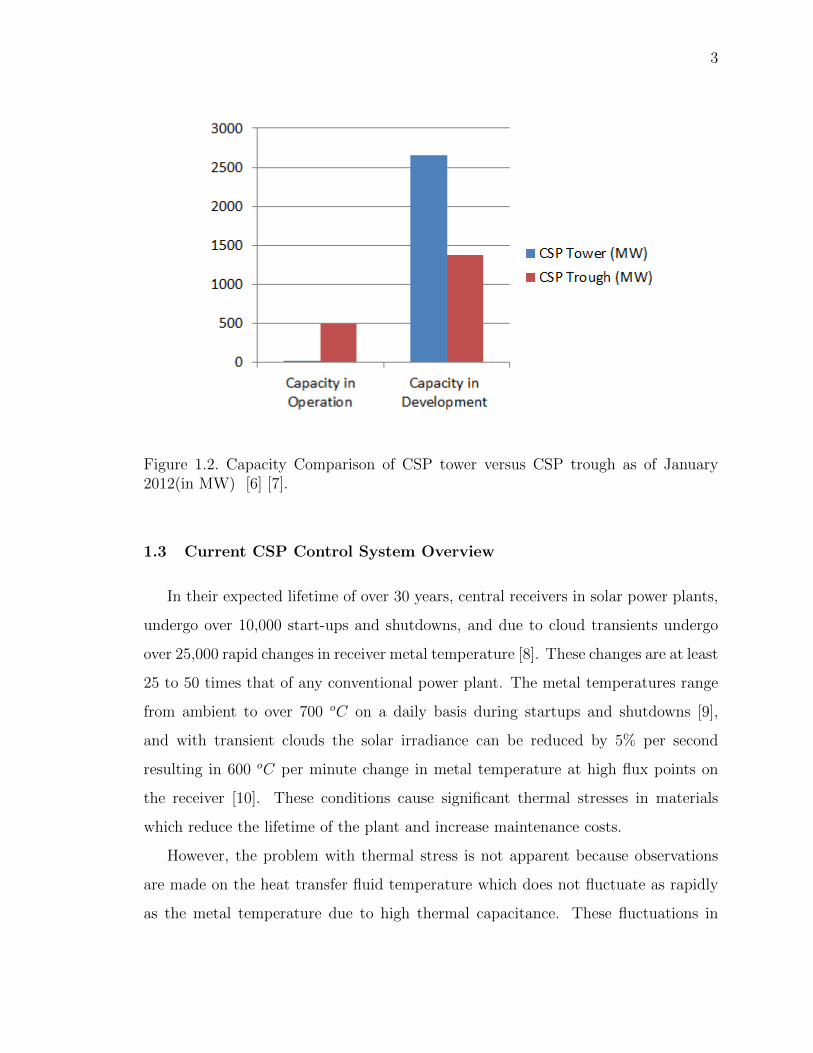
1.2 Capacity Comparison of CSP tower versus CSP trough as of January2012(in MW) [6] [7]. . . . . . . . . . . . . . . . . . . . . . . . . . . . . 3
2.1 Heliostat field layout [17]. . . . . . . . . . . . . . . . . . . . . . . . . . 7
2.2 Heliostat field position [19]. . . . . . . . . . . . . . . . . . . . . . . . . 8
2.3 Altitude azimuth tracking geometry [21]. . . . . . . . . . . . . . . . . . 8
2.4 Intersection geometry of heliostat [19]. . . . . . . . . . . . . . . . . . . 9
2.5 Flow path of working fluid inside CSP receiver. . . . . . . . . . . . . . 11
2.6 Panel Structure. . . . . . . . . . . . . . . . . . . . . . . . . . . . . . . . 12
2.7 ith node micro-structure of panel. . . . . . . . . . . . . . . . . . . . . . 13
2.8 Schematic illustration of a TES thermocline, [27]. . . . . . . . . . . . . 16
2.9 Schematic illustration of steam turbine power generation system. . . . 22
2.10 Schematic illustration of temperature distribution in steam turbine powergeneration system. . . . . . . . . . . . . . . . . . . . . . . . . . . . . . 23
2.11 Schematic illustration of boiler system [41]. . . . . . . . . . . . . . . . . 23
3.1 CSP Control Schematic. . . . . . . . . . . . . . . . . . . . . . . . . . . 33
3.2 Typical CSP operation scenarios. . . . . . . . . . . . . . . . . . . . . . 33
3.3 Optimized heliostat field position. . . . . . . . . . . . . . . . . . . . . . 38
3.4 Equilibrium nodes tube and HTF temperature with u∗1 = 450kg/s. . . . 43
3.5 HTF outlet temperature and controller output with LQR. . . . . . . . 44
3.6 Receiver tube inlet temperature and outlet temperature with LQR. . . 44
3.7 Equilibrium map candidate. . . . . . . . . . . . . . . . . . . . . . . . . 48
3.8 Discharge-charging cycle (Re = 240, Ψ = 150), H = 1.0C0, [27]. . . . . 48
3.9 Drum pressure for constant flow rate and energy step input. . . . . . . 50
viii
Figure Page
3.10 Control schematic for steam turbine generator system. . . . . . . . . . 51
3.11 Output active power from generator and mechanical power input to thesteam turbine generator system with controllers in pu. . . . . . . . . . 52
3.12 Speed deviation for the turbines and generator and torques between turbines-generator. . . . . . . . . . . . . . . . . . . . . . . . . . . . . . . . . . . 52
4.1 Kalman filter schematic for receiver dynamics with small disturbance . 57
4.2 LQG regulator schematic for receiver dynamics with small disturbance 60
4.3 Disturbance/Measurement noise level and HTF outlet temperature withLQG regulator design . . . . . . . . . . . . . . . . . . . . . . . . . . . . 62
4.4 LQI controller schematic for receiver dynamics with small disturbance 64
4.5 LQG reference controller schematic for receiver dynamics with small dis-turbance . . . . . . . . . . . . . . . . . . . . . . . . . . . . . . . . . . 64
4.6 LQG regulator schematic for receiver dynamics with small disturbance 65
5.1 Instant thermal strain of inlet and outlet headers with LQR shown inFigure 3.6. . . . . . . . . . . . . . . . . . . . . . . . . . . . . . . . . . . 69
5.2 Relationship between HTF outlet temperature deviation r and maximuminstant thermal strain εmax. . . . . . . . . . . . . . . . . . . . . . . . . 70
5.3 Load/Price calibration and forecast. . . . . . . . . . . . . . . . . . . . 71
5.4 Load forecast and MAPE evaluation for neural network prediction model(12/15/2008-12/29/2008). . . . . . . . . . . . . . . . . . . . . . . . . . 73
5.5 Load forecast and MAPE evaluation for bagged regression tree predictionmodel (12/15/2008-12/29/2008). . . . . . . . . . . . . . . . . . . . . . 76
5.6 Load forecast regression tree structure, prune to level 5. . . . . . . . . 77
5.7 Predictor weight of load forecast bagged regression tree. . . . . . . . . 77
5.8 Load forecast bagged regression tree, Out-of-Bag regression error as func-tion of No. of grown trees. . . . . . . . . . . . . . . . . . . . . . . . . . 78
A.1 Solar radiation for days with and without cloud. . . . . . . . . . . . . . 87
A.2 Frequency response of photoelectric detectors. . . . . . . . . . . . . . . 88
A.3 Plot of concentrated sunshine on a target using Beam CharacterizationSystem. . . . . . . . . . . . . . . . . . . . . . . . . . . . . . . . . . . . 89

ix
ABSTRACT
Luo, Qi. Ph.D, Purdue University, May 2015. Control Oriented Concentrating SolarPower (CSP) Plant Model and its Applications. Major Professor: Kartik Ariyur,School of Mechanical Engineering.
Solar receivers in concentrating solar thermal power plants (CSP) undergo over
10,000 start-ups and shutdowns, and over 25,000 rapid rate of change in temperature
on receivesr due to cloud transients resulting in performance degradation and material
fatigue in their expected lifetime of over 30 years. The research proposes to develop a
three-level controller that uses multi-input-multi-output (MIMO) control technology
to minimize the effect of these disturbances, improve plant performance, and extend
plant life. The controller can be readily installed on any vendor supplied state-of-the-
art control hardware.
We propose a three-level controller architecture using multi-input-multi-output
(MIMO) control for CSP plants that can be implemented on existing plants to improve
performance, reliability, and extend the life of the plant. This architecture optimizes
the performance on multiple time scalesreactive level (regulation to temperature set
points), tactical level (adaptation of temperature set points), and strategic level (trad-
ing off fatigue life due to thermal cycling and current production). This controller
unique to CSP plants operating at temperatures greater than 550 oC, will make CSPs
competitive with conventional power plants and contribute significantly towards the
Sunshot goal of 0.06/kWh(e), while responding with agility to both market dynamics
and changes in solar irradiance such as due to passing clouds. Moreover, our develop-
ment of control software with performance guarantees will avoid early stage failures
and permit smooth grid integration of the CSP power plants. The proposed controller
can be implemented with existing control hardware infrastructure with little or no
additional equipment.

x
In the thesis, we demonstrate a dynamics model of CSP, of which different com-
ponents are modelled with different time scales. We also show a real time control
strategy of CSP control oriented model in steady state. Furthermore, we shown dif-
ferent controllers design for disturbance rejection and reference tracking to handle
complex receiver dynamics under system disturbance and measurement noise. At
last, we show different applications of this control oriented CSP model including life
cycle enhancement and electricity load forecasting using both neural network and
regression tree.

1
1. BACKGROUND AND MOTIVATION
1.1 Solar Energy Overview
According to technical report from National Renewable Energy Laboratory [1],
solar energy technologies is still at unprecedented levels, with significant aids by the
advent of utility-scale projects which sell their power directly to the utilities. These
systems, compared with the traditional solar energy projects, can achieve significant
economics of scale in operation, therefore reduce the cost of delivered power.
Based on database maintained by Solar Energy Industries Association [2], [3],
there are around 16,043 megawatts(MW) of utility-scale solar resources under devel-
opment within United States, of which photovoltaic(PV) projects make up 72% of the
total project, and concentrating solar plant (CSP), which includes both CSP tower
and CSP troughs, take 25% of the market share, as shown in figure 1.1.
1.2 CSP Tower Market and Technology Overview
CSP tower systems, often referred to as power towers or central receivers, are
composed of four subsystems:
• Field of Heliostats.
• CSP receiver.
• Thermal storage.
• Steam turbine system.

2
Figure 1.1. Total U.S. utility-scale solar capacity solar capacity under development(in MW) [1].
Upon operation, the field of heliostats will track the sunshine and redirect it to
the receiver on top of a tower, the concentrated rate of the sunshine can usually be
over 600 times, and therefore can heat transfer fluid ( Usually steam, air, molten salt,
etc.) up to 500 o to 850 o, the heated fluid will usually be used to serve as heat source
of steam turbine, or to be stored in thermal storage system for further usage [4].
Of the total 1176 MW utility scale solar power under operation by January 2012,
about 503 MW is by CSP facilities, and only 10 MW is by CSP tower [5], compared
with 493 MW of CSP trough. However, the total capacity of CSP tower under
development (2655 MW) is significant higher than the capacity of CSP trough under
development (1375 MW), as shown in figure 1.2.
3
Figure 1.2. Capacity Comparison of CSP tower versus CSP trough as of January2012(in MW) [6] [7].
1.3 Current CSP Control System Overview
In their expected lifetime of over 30 years, central receivers in solar power plants,
undergo over 10,000 start-ups and shutdowns, and due to cloud transients undergo
over 25,000 rapid changes in receiver metal temperature [8]. These changes are at least
25 to 50 times that of any conventional power plant. The metal temperatures range
from ambient to over 700 oC on a daily basis during startups and shutdowns [9],
and with transient clouds the solar irradiance can be reduced by 5% per second
resulting in 600 oC per minute change in metal temperature at high flux points on
the receiver [10]. These conditions cause significant thermal stresses in materials
which reduce the lifetime of the plant and increase maintenance costs.
However, the problem with thermal stress is not apparent because observations
are made on the heat transfer fluid temperature which does not fluctuate as rapidly
as the metal temperature due to high thermal capacitance. These fluctuations in

4
fluid temperature are tolerated because they do not significantly impact performance
and hence the open control strategies that to control heliostats and simple feedback
control by manipulating flow rate to maintain heat transfer fluid temperature appear
acceptable.
The fossil power plant industry knows that during every startup and shutdown
process, the parts along hot fluid path suffer significant thermal cycling. The life cycle
of those parts may be shorten due to the thermal cycling. This can result in a plant
cost increase in two ways: First more parts have to be replaced during the inspections,
which increase the plant maintenance cost. Second, since the parts maintenance cost
get paid out earlier, this cost would have an additional cost increase due to the time
value of money. Babcock & Wilcox study using BLESS code (boiler life evaluation
and simulation system) and temperature vs time history of metal on headers showed
that reducing the temperature imbalance in headers from 30oC to 15oC extends life
by 3000 hours [11]. Prior control studies with solar central receiver showed that a
different control strategy must be used during cloud transients. Further, this study
found that the receiver flow patterns must be designed to include crossover from east
to west side of receiver to minimize the temperature imbalance due to change in heat
flux on these sides as the sun moves in the sky from east to west during the course of
the day. These modifications are implemented in CSP systems that are being built.
Grossman et al [12] developed correlations for the reduction in life time caused by
creep-fatigue damage during thermal cycling.
1.4 Benefits and Motivation for New Multiple Input Multiple Output
(MIMO) Controller
1. First Costs Reduction, Better Bankability, and Lower Levelized Energy Cost
(LCOE).
(a) Systems with simple controls are typically designed to run significantly be-
low the maximum capability to avoid violating the maximum constraints

5
on temperatures or pressures. Advance control such as the proposed MIMO
control, guarantee that these constraints are not violated, thus allowing
the plant to operate closer to constraint boundaries and resulting in bet-
ter output or efficiency point. For example, receiver fluid temperatures
are designed to withstand temperatures of upto 600oC but the maximum
operating point is specified as 565oC to allow for a safety margin. It is
possible to increase this temperature to 580oC with MIMO controller re-
sulting in improving turbine generation efficiency by 1.1% and reducing
first costs for the same rated capacity or improving energy output.
(b) With MIMO controller, we can better control the temperatures and rates
of change of temperature. Material specifications and/or design safety
factors can be relaxed, thus reducing first costs.
A trade-off between capital savings in (a) or (b) can be made.
2. Operating Cost Reduction
(a) With the proposed controller, thermal stress is explicitly controlled within
specified limits. This will reduce metal fatigue and creep, fewer failures
and better maintained assets which will result in reduced part replacement,
improved availability, reduced maintenance costs and extended plant life.
Reducing these costs impact the time it takes for the CSP system to reach
profitability.
(b) With the proposed controller, market-decision making mechanism can be
integrated with current CSP plant, increasing the automation in energy
market biding and plant production planning.

6
2. CONTROL ORIENTED MODEL
As mentioned in chapter 1, the overall schematic of concentrating solar plant and
corresponding control objective, as shown in figure 3.1, is composed of four parts:
2.1 Field of Heliostats
In the power tower system , the low dense solar radiation is reflected and concen-
trated over 500 times by a series of mirror called heliostats to the receiver of system,
where the concentrated solar radiation can be absorbed and translated into thermal
power to and used to generate electricity. The heliostat field is important subsystem
because it is worth 50% of the total CSP system cost [13], and around 49% of the
total system energy lost [14]. The control and optimization problems related to the
subsystem are:
2.1.1 Location–Altitude,Azimuth Relation
The objective is to compute the sun position (zenith and azimuth angle at the
observer location) as a function of the observer local time and position as discussed by
Reda and Andreas [15], for calculation reference in heliostat field layout optimization
and heliostat position control.
2.1.2 Field layout optimization
The significant factors affecting the performance of central receiver solar thermal
systems including, (i) cosine losses, (ii) shading and blocking, (iii) receiver interception
(i.e., heat not lost due to spillage), (iv) atmospheric attenuation between heliostat
and receiver, and (v) heliostat reflectivity, as discussed in Schmitz et al’s work [16].
7
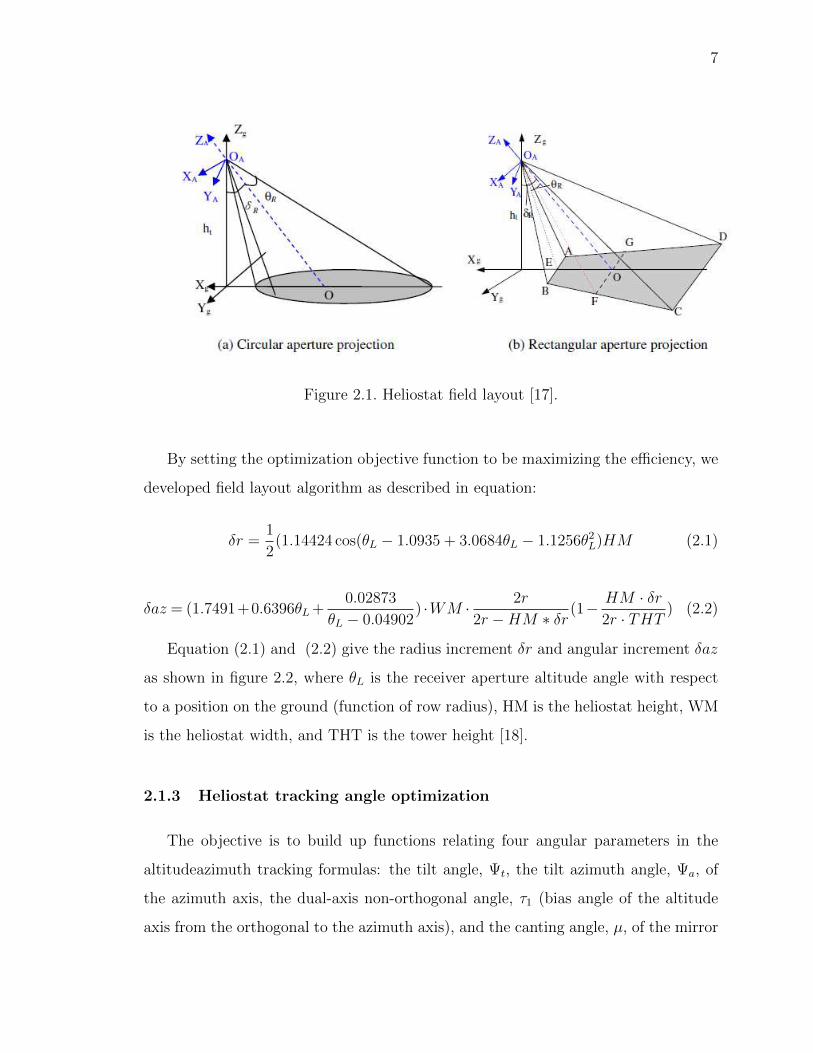
Figure 2.1. Heliostat field layout [17].
By setting the optimization objective function to be maximizing the efficiency, we
developed field layout algorithm as described in equation:
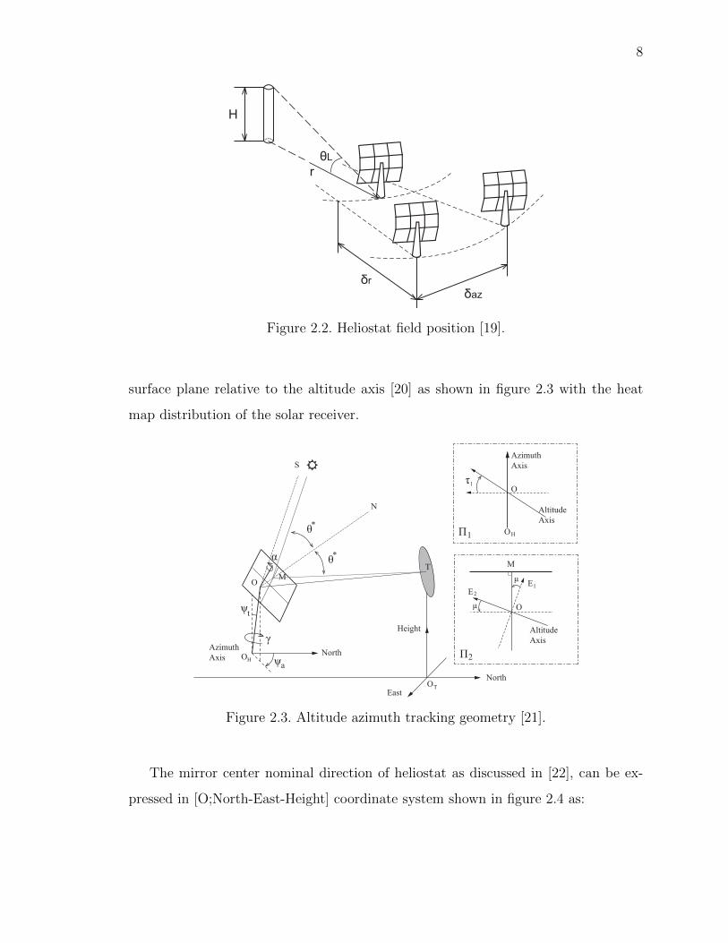
δr =1
2(1.14424 cos(θL − 1.0935 + 3.0684θL − 1.1256θ2L)HM (2.1)
(2.2)δaz = (1.7491+0.6396θL+0.02873
θL − 0.04902) ·WM · 2r
2r −HM ∗ δr(1− HM · δr
2r · THT)
Equation (2.1) and (2.2) give the radius increment δr and angular increment δaz
as shown in figure 2.2, where θL is the receiver aperture altitude angle with respect
to a position on the ground (function of row radius), HM is the heliostat height, WM
is the heliostat width, and THT is the tower height [18].
2.1.3 Heliostat tracking angle optimization
The objective is to build up functions relating four angular parameters in the
altitudeazimuth tracking formulas: the tilt angle, Ψt, the tilt azimuth angle, Ψa, of
the azimuth axis, the dual-axis non-orthogonal angle, τ1 (bias angle of the altitude
axis from the orthogonal to the azimuth axis), and the canting angle, µ, of the mirror
8
r
δr
δaz
H
θL
Figure 2.2. Heliostat field position [19].
surface plane relative to the altitude axis [20] as shown in figure 2.3 with the heat
map distribution of the solar receiver.
ψa
γ
North
North
EastOT
OM
α θ*
θ*
S
N
T
Height
Azimuth
Axis OH
ψt
M
Altitude
Axis
O
EE2
1
μ
μ
Altitude
Axis
O
Azimuth
Axis
1τ
П1
П2
OH
Figure 2.3. Altitude azimuth tracking geometry [21].
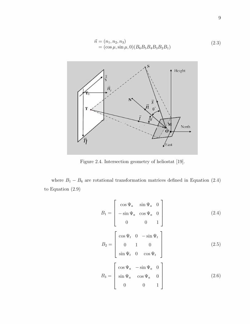
The mirror center nominal direction of heliostat as discussed in [22], can be ex-
pressed in [O;North-East-Height] coordinate system shown in figure 2.4 as:
9
(2.3)~n = (n1, n2, n3)= (cosµ, sinµ, 0)(B6B5B4B3B2B1)
Figure 2.4. Intersection geometry of heliostat [19].
where B1 − B6 are rotational transformation matrices defined in Equation (2.4)
to Equation (2.9)
B1 =
cos Ψa sin Ψa 0
− sin Ψa cos Ψa 0
0 0 1
(2.4)
B2 =
cos Ψt 0 − sin Ψt
0 1 0
sin Ψt 0 cos Ψt
(2.5)
B3 =
cos Ψa − sin Ψa 0
sin Ψa cos Ψa 0
0 0 1
(2.6)
10
B4 =
cos γ sin γ 0
− sin γ cos γ 0
0 0 1
(2.7)
B5 =
1 0 0
0 cos τ1 sin τ1
0 − sin τ1 cos τ1
(2.8)
B6 =
1 0 0
0 cos τ1 sin τ1
0 − sin τ1 cos τ1
(2.9)
Solar vector can be expressed as in Equation (2.10).
~s = (cosα cos γ, cosα sin γ, sin γ) (2.10)
where α is solar altitude angle, and γ is solar azimuth angle.
2.2 CSP Tower
CSP tower, or called CSP receiver, have been studies for years. The majority
heat loss from receiver are from reflected radiation, emitted radiation, conduction
and convection, as discussed in [23], and detailed heat loss analysis of various types
of receivers with air, steam and molten salt as working fluid have also been discussed
fully by researchers as well. [24], [25], [26],
2.2.1 CSP structural analysis
Solar image on the surface of the CSP receiver is usually symmetrical for one or
two axis, depending on the heat map desired. Total heat transfer fluid (HTF) is
usually separated into two geographically symmetrical and independent flow circuit.
11
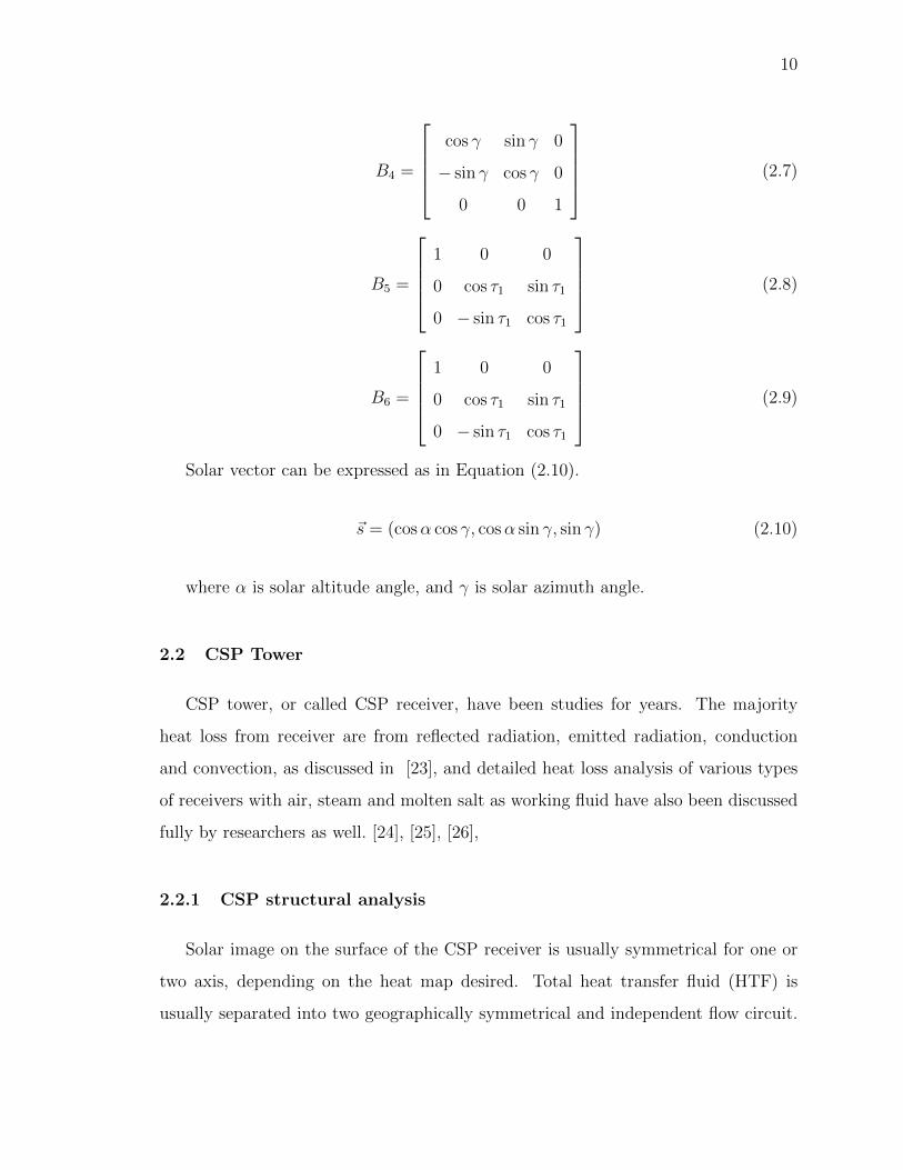
The fluid flow dynamics would be arrange accordingly. The example we discuss
is one-axis symmetrical along north-south direction, dividing the heat map of CSP
receiver into east part and west part. In this scenario, we present CSP receiver flow
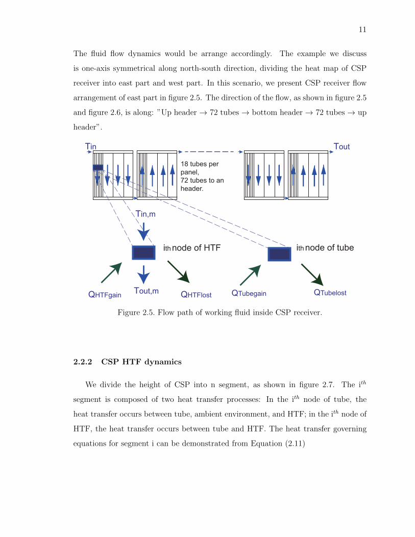
arrangement of east part in figure 2.5. The direction of the flow, as shown in figure 2.5
and figure 2.6, is along: ”Up header→ 72 tubes→ bottom header→ 72 tubes→ up
header”.
Tin
Tin,m
Tout,m
Tout
QHTFgain QHTFlost QTubegain QTubelost
ith node of HTF ith node of tube
18 tubes per
panel,
72 tubes to an
header.
Figure 2.5. Flow path of working fluid inside CSP receiver.
2.2.2 CSP HTF dynamics
We divide the height of CSP into n segment, as shown in figure 2.7. The ith
segment is composed of two heat transfer processes: In the ith node of tube, the
heat transfer occurs between tube, ambient environment, and HTF; in the ith node of
HTF, the heat transfer occurs between tube and HTF. The heat transfer governing
equations for segment i can be demonstrated from Equation (2.11)
12
Figure 2.6. Panel Structure.
(mCp)tubedTt(i, j, k)
dt= Qinc(i, j, k)− (Qrad(i, j, k) +Qconv(i, j, k) +Qrefl(i, j, k))
− (UA)(Tt(i, j, k)− THTF (i, j, k))(2.11)
(mCp)HTFdTHTF (i, j, k)
dt= (UA)(Tt(i, j, k)− THTF (i, j, k))−QHTF (2.12)
where (mCp)tube is the mass times specific capacity of tube, (mCp)HTF is the mass
times specific heat capacity of working fluid, which are defined in Equation (2.13)
and (2.14)
(mCp)tube = π · dtube · 18 · dz · ttube · ρtube · CPtube (2.13)
(mCp)HTF = π · dtube · 18 · dz · ρHTF · CHTF (2.14)
Qinc(i, j, k) in Equation (2.11) is the energy absorbed due to incident of radiation
reflected by the heliostat to ith node on the jth panel of kth header on receiver.
13
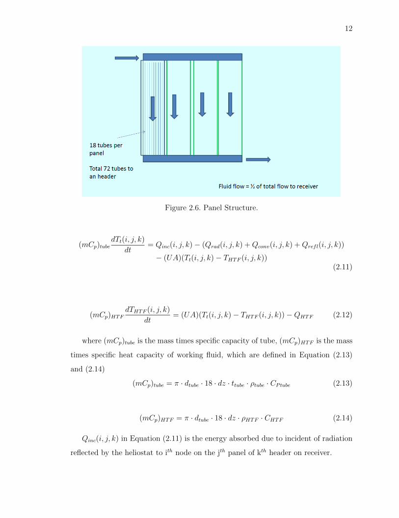
Figure 2.7. ith node micro-structure of panel.
U and A in Equation (2.11) and Equation (2.12) are convectional heat transfer
coefficient between tube and HTF and surface area of the node respectively. U and
A are defined in equation
U = U0 · (mHTF
mdesignHTF
)0.8 (2.15)
A = π · dtube · dz · 18 (2.16)
Qrad(i, j, k), Qconv(i, j, k) and Qrefl(i, j, k) are energy lost to ambient temperature
due to radiation, convectional and reflection respectively, defined in Equation (2.17)
to Equation (2.19).
14
Qrad(i, j, k) = σ · ε · f · A · (T 4t (i, j, k)− T 4
amb) (2.17)
Qconv(i, j, k) = hconv · (Tt(i, j, k)− Tamb) (2.18)
Qrefl(i, j, k) = 0 (2.19)
σ in Equation (2.17) is StefanBoltzmann constant, ε is emissivity, f is radiation
efficiency defined asQtube
rad
Qblackbodyrad
, Tamb is the ambient temperature. In Equation (2.18),
hconv is the convectional rate between tube and ambient temperature, here, loss due
to reflection Qrefl is relatively small that we can reasonably approximate it to 0.
2.3 Thermal Storage
The output of a simple solar-only power plant depends largely on the solar input
and weather condition, which, at most of the time, does not correspond with the
utility load profile. In order to facilitate the output of solar station to minimize
the weather influence, as well as to tail the plant output based on utility energy
consumption patter, thermal storage system (TES) has largely be applied integrated
in solar plants. By balancing the relationship between solar production and electricity
load, we can improve power operation efficiency, reduce operational and management
costs, and increase the stability of the system [27].
Thermal storage system usually use tank to store thermal energy. Inside the
tank, the hot fluid is separated from the cold fluid by applying thermal gradient and
heat transfer fluid (HTF) maintains high and low temperatures above and between
the thermocline, respectively. Usually lower-cost filter material is used to displace
high-cost fluid. [28]. There are two typical design options: two-tank storage, and
single-tank thermocline storage [29]. In the single-tank system, cold fluid enters from
the bottom, passes through CSP receiver and get heated, and eventually returns to
15
the top of the tank in the charging process. while in the discharing process, hot fluid
is drawn from the top and pushed through a heat exchanger to get cooled. In a
two-tank storage system, the molten-salt HTF flows from a cold tank to a hot tank
through CSP receiver at charging, and flows back from the hot tank to cold though
the steam generator at discharging cycle [30]. The advantage of single-tank system
is that it is approximately 35% of the double-tank system of same capacity [31], but
the latter has low-risk in energy storage since it separates the hot and cold fluid into
two different tanks.
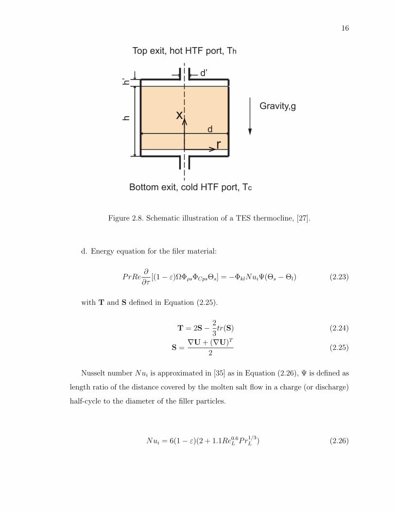
2.3.1 Thermal storage dynamics
The thermal storage dynamics equations has been developed by many researchers [32],
[33], [34], and here we present dimensional governing equations for continuity, mo-
mentum and energy are presented in [29], it is worth to point out that, the thermal
storage dynamics model in the paper are designed for CSP trough, but the model
can be easily embedded into CSP tower system as well. Zhen Yang and Suresh V.
Garimella’s work had been presented and embedded in the overall CSP [27].
a. Continuity equation:
ε∂Φρ
∂τ+∇ · (ΦρU) = 0 (2.20)
a. Momentum equation:
Re∂Φρ
∂τ+ReΨ∇ · (ΦρUU
ε) = −ε∇P +∇ ·T + εΦρGrex − ε(
ΨµU
Da2+FReΨ
DaΦρUU)
(2.21)
c. Energy equation for the molten salt:
(2.22)PrRe
∂
∂τ(−εΦρΦCplΘl) + PrRe∇ · (ΦρΦCplΘlU)
=1
Ψ∇ · (Φke∇Θl) + 2PrAReΦµ[SS′ + tr(S)tr(S′)] + ΦklNuiΨ(Θs −Θl)
16
x
r
dh
h’ d’
Gravity,g
Top exit, hot HTF port, Th
Bottom exit, cold HTF port, Tc
Figure 2.8. Schematic illustration of a TES thermocline, [27].
d. Energy equation for the filer material:
PrRe∂
∂τ[(1− ε)ΩΦρsΦCpsΘs] = −ΦklNuiΨ(Θs −Θl) (2.23)
with T and S defined in Equation (2.25).
T = 2S− 2
3tr(S) (2.24)
S =∇U + (∇U)T
2(2.25)
Nusselt number Nui is approximated in [35] as in Equation (2.26), Ψ is defined as
length ratio of the distance covered by the molten salt flow in a charge (or discharge)
half-cycle to the diameter of the filler particles.
Nui = 6(1− ε)(2 + 1.1Re0.6L Pr1/3L ) (2.26)
17
The non-dimensional parameters included in Equations (2.20) and (2.23) are
defined as in Equations (2.30) to (2.46):
τ =tVcd2s, (2.27)
X =x
ds, (2.28)
R =r
ds, (2.29)
U =u
um, (2.30)
H =h
ds, (2.31)
D =d
ds, (2.32)
D′ =d′
ds, (2.33)
18
Re =umdsvc
, (2.34)
P =pd
µcum, (2.35)
Gr =gd2svcum
, (2.36)
Da =
√K
ds, (2.37)
A =u2m
Cplc(Th − Tc), (2.38)
Nui =hid
2s
kls, (2.39)
Pr =vcαc, (2.40)
Pr =CPlcµ
klc, (2.41)
19
Θl =Tl − TcTh − Tc
, (2.42)
Θs =Ts − TcTh − Tc
, (2.43)
Ω =ρscCPscρlcCPls
, (2.44)
¯T =¯τdsµum
, (2.45)
∇ = ex∂
∂X+ e`
∂
∂θ+ er
∂
∂R(2.46)
Coefficient Φρ,Φmu,ΦCpl,Φkl, Φke, Φρs and ΦCps represents the density, viscosity,
specific heat, thermal conductivity, effective thermal conductivity, of molten salt, and
density and specific heat of filter material, respectively, and expressed as in equation,
and is fits nicely with data indicated in [36]
Φρ = 1− 0.732(Th − Tc)2084.4− 0.732Tc
ΘI (2.47)
Φµ =exp−4.343− 2.0143ln[(Th − Tc)ΘI + Tc] + 10.094
exp−4.343− 0.20143lnTc + 10.094(2.48)
20
Φkl =−6.52× 10⁻⁴[(Th − Tc)Θl + Tc] + 0.5908
−6.53× 10⁻⁴Tc + 0.5908(2.49)
ΦCpl = 1 (2.50)
ΦCps = 1 (2.51)
Φρs = 1 (2.52)
Φke = Φkl1 + 2βφ+ (2β3 − 0.1β)φ2 + φ30.05 exp 4.5β
1− βθ(2.53)
where we have θ and β in Equation (2.53) defined as in Equation (2.55), as dis-
cussed in [37].
θ = 1− ε (2.54)
β =ks − klks + 2kl
(2.55)
Assume the inlet and outlet flow are of uniform temperature, with boundary
condition defined as
• At the top exit of the filler bed in the discharge half-cycle when (0 < τ < 1):
U = ex (2.56)
∂Θl
∂X= 0 (2.57)

21
• At the top exit of the filler bed in the charge half-cycle when (1 < τ < 2):
U = −ex (2.58)
Θl = 1 (2.59)
• At the bottom exit of the filler bed in the discharge half-cycle when (0 < τ < 1):
∂U
∂X= 0 (2.60)
Θl = 0 (2.61)
• At the bottom exit of the filler bed in the charge half-cycle when (1 < τ < 2):
∂U
∂X= 0 (2.62)
∂Θl
∂X= 0 (2.63)
2.4 Steam Turbine Electricity Generation System
The steam turbines have been widely employed since almost one century ago to
power generating due to their efficiencies and costs.
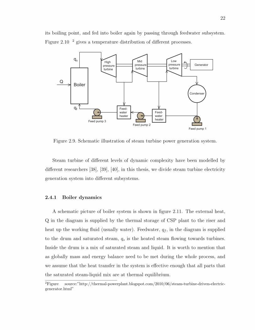
Figure 2.9 1 gives a two level turbine electricity generation system, the high pres-
sure steam comes from boiler, and is fed into turbine, in which it passes along the
alternatively fixed and moving blades, from inlet port to outlet port, the cavity be-
tween blades and turbine are therefore increasing, causing a drop of steam pressure
and an increase in kinetic energy of steam, the moving steam impacts on the rota-
tional blades and transfer parts of its kinetic energy to these blades. The steam from
outlet is fed into secondary turbine again, repeat the process, causing the drop of
temperature and pressure of steam again. The outlet steam from the secondary tur-
bine goes into condenser, in which the temperature of steam usually dropped below
1Figure source:”http://thermal-powerplant.blogspot.com/2010/06/steam-turbine-driven-electric-generator.html”
22
its boiling point, and fed into boiler again by passing through feedwater subsystem.
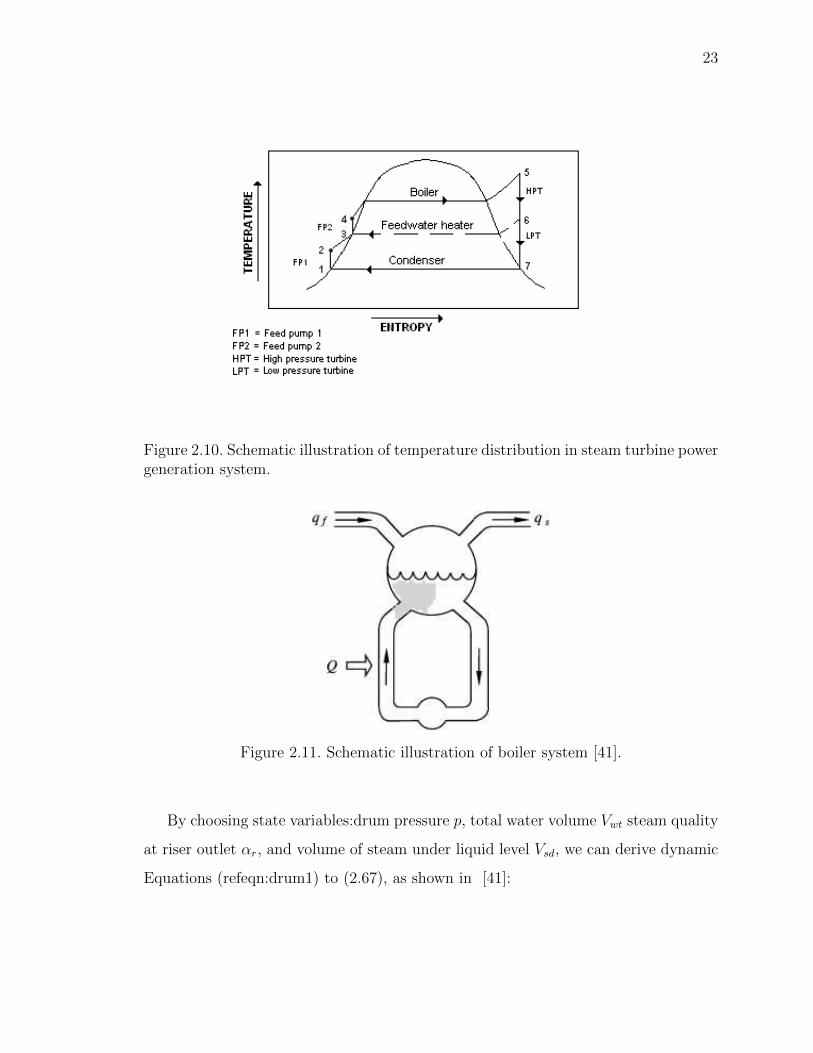
Figure 2.10 2 gives a temperature distribution of different processes.
Boiler
High
pressure
turbine
Mid
pressure
turbine
Low
pressure
turbineGenerator
Feed-
water
heater
Feed-
water
heaterFeed pump 3
Feed pump 1
Condenser
Q
qs
qf
Feed pump 2
Figure 2.9. Schematic illustration of steam turbine power generation system.
Steam turbine of different levels of dynamic complexity have been modelled by
different researchers [38], [39], [40], in this thesis, we divide steam turbine electricity
generation system into different subsystems.
2.4.1 Boiler dynamics
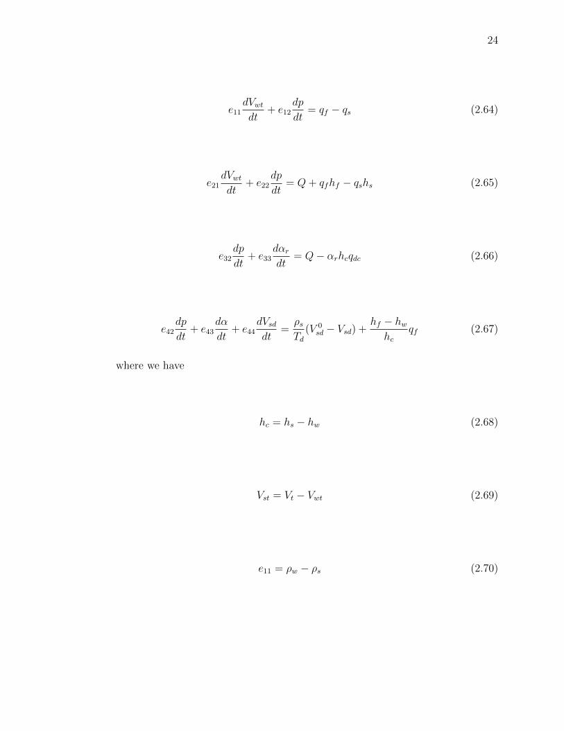
A schematic picture of boiler system is shown in figure 2.11. The external heat,
Q in the diagram is supplied by the thermal storage of CSP plant to the riser and
heat up the working fluid (usually water). Feedwater, qf , in the diagram is supplied
to the drum and saturated steam, qs is the heated steam flowing towards turbines.
Inside the drum is a mix of saturated steam and liquid. It is worth to mention that
as globally mass and energy balance need to be met during the whole process, and
we assume that the heat transfer in the system is effective enough that all parts that
the saturated steam-liquid mix are at thermal equilibrium.
2Figure source:”http://thermal-powerplant.blogspot.com/2010/06/steam-turbine-driven-electric-generator.html”
23
Figure 2.10. Schematic illustration of temperature distribution in steam turbine powergeneration system.
Figure 2.11. Schematic illustration of boiler system [41].
By choosing state variables:drum pressure p, total water volume Vwt steam quality
at riser outlet αr, and volume of steam under liquid level Vsd, we can derive dynamic
Equations (refeqn:drum1) to (2.67), as shown in [41]:
24
e11dVwtdt
+ e12dp
dt= qf − qs (2.64)
e21dVwtdt
+ e22dp
dt= Q+ qfhf − qshs (2.65)
e32dp
dt+ e33
dαrdt
= Q− αrhcqdc (2.66)
e42dp
dt+ e43
dα
dt+ e44
dVsddt
=ρsTd
(V 0sd − Vsd) +
hf − hwhc
qf (2.67)
where we have
hc = hs − hw (2.68)
Vst = Vt − Vwt (2.69)
e11 = ρw − ρs (2.70)

25
e12 = Vwt∂ρw∂p
+ Vst∂ρs∂p
(2.71)
e21 = ρwhw − ρshs (2.72)
e22 = Vwt(hw∂ρw∂p
+ Vst(hs∂ρs∂p
+ ρs∂hs∂p
)− Vt +mtCp∂ts∂p
(2.73)
(2.74)e32 = (ρw
∂hw∂p− αrhc
∂ρw∂p
)(1− αv)Vr + (1− αr)hc∂ρs∂p
+ ρs∂hs∂p
)αvVr
+ (ρs + (ρw − ρs)αr)hcVr∂αv∂p
− Vr+mrCp
∂ts∂p
e33 = ((1− αr)ρs + αrρw)hcVr∂αv∂αr
(2.75)
(2.76)e42 = Vsd
∂ρs∂p
+1
hc(ρsVsd
∂hs∂p
+ ρwVwd∂hw∂p− Vsd − Vwd +mdCp
∂ts∂p
)
+ αr(1 + β)Vr(αv∂ρs∂p
+ (1− αv∂ρw∂p
+ (ρs − ρw)∂αv∂p
)
e43 = αr(1 + β)(ρs − ρw)Vr∂αv∂αr
(2.77)
26
e44 = ρs (2.78)
where in Equation (2.64) to Equation (2.78), V denote the volume, ρ specific
density, u specific internal energy, h specific enthalpy, t temperature, q mass flow
rate, and subscripts s, w, f, and m refer to steam, water, feedwater and metal, dou-
ble subscripts t denotes total system, d drum and r riser. αv and qdc are given in
Equation (2.79) and (2.80).
αv =ρwρwρs
(1− ρs(ρw − ρs)αr
ln(1 +ρw − ρsρs
αr)) (2.79)
qdc =
√2ρwAdc(ρw − ρs)gαvVr
k(2.80)
2.4.2 Steam turbine dynamics
Based on previous work done by Lin and Tsai [42], the steam turbine-generator
unit has very complex mechanical characteristics. Here we can simplify the models
to the lumped mass-damping-spring model shown in following equations:
JiBdωiBdt
= τiB −DiBωiB −KiB(θiB − θi) (2.81)
i = H,M,L (2.82)
The turbine rotor dynamics are as follows:
JHdωHdt
= τH −DHωH −KHM(θH − θM)−KHB(θH − θHB) (2.83)
27
(2.84)JMdωMdt
= τM −DMωM −KML(θM − θL)−KHM(θM − θH)−KMB(θM − θMB)
(2.85)JLdωLdt
= τL −DLωL −KLG(θL − θG)−KML(θL − θM)−KLB(θL − θLB)
The generator rotor dynamic equation is as follows
(2.86)JGdωGdt
= τEM −DGωG −KLG(θG − θL)
The symbols J, K, D, T, v and u, respectively, represent the inertia constant,
stiffness coefficient, damping coefficient, torque, angular velocity and angle. The
subscripts H, M, L, G and B, respectively, represent high-pressure turbine rotor, mid-
pressure turbine rotor, low-pressure turbine rotor, generator and blade. The τEM
represents the electromagnetic torque of the generator.
2.4.3 Synchronous generator circuit model
The d-q dynamic model for three-phase windings and excitation windings, as
discussed by Ewald and Mohammad [43], is shown in following equations:
vds = (ωrωbXq)iqs + (−rs −
p
ωbXd)ids + (
p
ωbXmd)i
′
fd (2.87)
vqs = (−rs −p
ωbXq)iqs + (−ωr
ωbXd)ids + (
ωrωbXmd)i
′fd (2.88)
τEM = (3
2)(P
2)[Lmdi
′fdiqsids + (Lmq − Lmd)iqsids] (2.89)
where P is the number of poles, vds is direct axis voltage, vqs is quadrature axis
voltage, vr is mechanical angular velocity, vb is rated system angular velocity, Xq is
quadrature axis reactor, Xd is direct axis reactor, Xmd is direct axis mutual reactor,
iqs is quadrature axis current, ids is direct axis current, ifd is field current, rs is
stator resistance, Lmd is direct axis mutual inductance, Lmq is quadrature axis mutual
inductance.

28
3. REAL TIME CONTROL FOR STEADY STATE OPERATION
3.1 Three-level MIMO Controller Introduction
In order to address problem of creep-fatigue damage on the CSP receiver, as well as
integrate market-decision control in the current CSP system. We propose three-level
MIMO controller (referred to as the controller) that will build on previous work in
model predictive and state feedback control and insights gained at Solar Two on effects
of thermal cycling on creep-fatigue damage on receiver. The controller will explicitly
take the rate-of-change of metal temperature and trade-off plant performance to help
calculate the best control moves and minimize the burden on the operator diurnal
startups and shutdowns and nominal cycling of loads.
The controller deals with the dynamics at different timescales - hours for mar-
ket conditions to minutes for cloud transients and to seconds for metal temperature
changes. For example, we propose to develop a MIMO controller with robust model
matching and with full state estimation in real-time (seconds) to regulate tempera-
ture and thereby bound propagation of demand disturbances into the tactical control
system; the tactical level adapts temperature set points (minutes) to minimize the
propagation of solar irradiance uncertainties into strategic decision-making control.
The strategic level (hours) in turn, trades off capital and production costs and suit-
ably negotiates pricing with the grid operator. Table 3.1 gives a general operation
time for gird control of different time scales, which, sets up a reactive time constrain
in control of CSP. In particular, the milliseconds to seconds level simulations are
important since:

29
• The milliseconds to seconds level model can capture the real time disturbance
and transient system dynamics changes.
• With the captured system change, with the milliseconds to seconds level model,
we can also analysis the how the transient disturbance and dynamics could be
propagated to the tactical level (seconds to minutes level) and the strategy level
( minutes to hours level).
• Based on the analysis of result (i.e. how the milliseconds level disturbance and
dynamics change would affect the life time, system profit, etc.) We can adapt
the milliseconds to seconds level control algorithm to minimize the error or
disturbance propagated up.
The controller uses mathematical models of differing sophistication at each time-
scale: non-linear distributed dynamic models for thermal stress cycling in the receiver,
lumped nonlinear thermo-hydraulic models (for example, receiver thermal dynamics,
drum boiler dynamics), semi-empirical models with parameter estimation for real-
time control, empirical correlations to make strategic operating decisions via hedg-
ing/market algorithms.
3.2 State of Development of the Controller and Proposed Approach
The following is the starting point for this project:
• A multi state non-linear dynamic model of the solar central receiver.
• A lumped parameter model dynamic model of the power generation system
including steam drum, superheater and molten salt loop dynamics.
• The control algorithms for the power block, thermal storage system, and cylin-
drical receiver.
• Baseline plant control structure, component dynamic models, and plant design
point parameters.
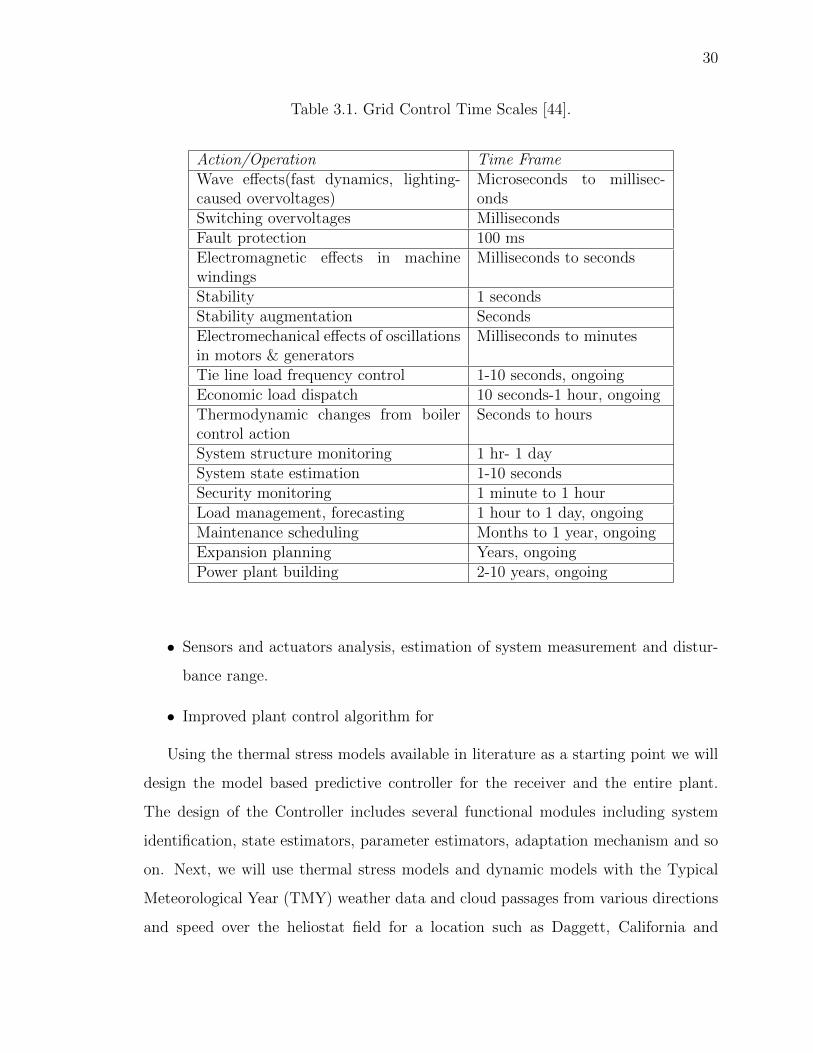
30
Table 3.1. Grid Control Time Scales [44].
Action/Operation Time FrameWave effects(fast dynamics, lighting-caused overvoltages)
Microseconds to millisec-onds
Switching overvoltages MillisecondsFault protection 100 msElectromagnetic effects in machinewindings
Milliseconds to seconds
Stability 1 secondsStability augmentation SecondsElectromechanical effects of oscillationsin motors & generators
Milliseconds to minutes
Tie line load frequency control 1-10 seconds, ongoingEconomic load dispatch 10 seconds-1 hour, ongoingThermodynamic changes from boilercontrol action
Seconds to hours
System structure monitoring 1 hr- 1 daySystem state estimation 1-10 secondsSecurity monitoring 1 minute to 1 hourLoad management, forecasting 1 hour to 1 day, ongoingMaintenance scheduling Months to 1 year, ongoingExpansion planning Years, ongoingPower plant building 2-10 years, ongoing
• Sensors and actuators analysis, estimation of system measurement and distur-
bance range.
• Improved plant control algorithm for
Using the thermal stress models available in literature as a starting point we will
design the model based predictive controller for the receiver and the entire plant.
The design of the Controller includes several functional modules including system
identification, state estimators, parameter estimators, adaptation mechanism and so
on. Next, we will use thermal stress models and dynamic models with the Typical
Meteorological Year (TMY) weather data and cloud passages from various directions
and speed over the heliostat field for a location such as Daggett, California and
31
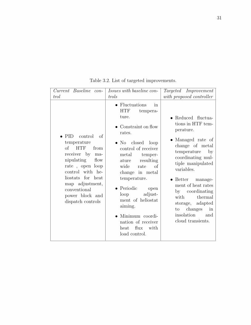
Table 3.2. List of targeted improvements.
Current Baseline con-trol
Issues with baseline con-trols
Targeted Improvementwith proposed controller
• PID control oftemperatureof HTF fromreceiver by ma-nipulating flowrate , open loopcontrol with he-liostats for heatmap adjustment,conventionalpower block anddispatch controls
• Fluctuations inHTF tempera-ture.
• Constraint on flowrates.
• No closed loopcontrol of receivermetal temper-ature resultingwide rate ofchange in metaltemperature.
• Periodic openloop adjust-ment of heliostataiming.
• Minimum coordi-nation of receiverheat flux withload control.
• Reduced fluctua-tions in HTF tem-perature.
• Managed rate ofchange of metaltemperature bycoordinating mul-tiple manipulatedvariables.
• Better manage-ment of heat ratesby coordinatingwith thermalstorage, adaptedto changes ininsolation andcloud transients.
32
show that stress or metal strain is reduced. To calculate the remaining life of the
component, we will use correlations from published literature such as Babcock and
Wilcox method [45] using BLESS models. The value of the life-extension will then be
calculated using the amount of additional electricity generated and Sunshot specific
cost of electricity [46] ($0.06 per kWh). A list of targeted improvements is shown in
Table 3.2.
3.3 Technical Details of the Proposed Approach
We aim to automate control and optimization of the entire plant and provide
specific guarantees for performance and safety at all time-scales of operation, integrate
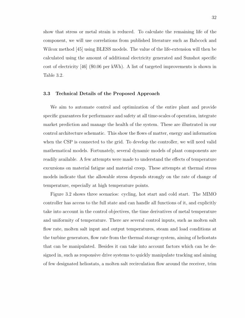
market prediction and manage the health of the system. These are illustrated in our
control architecture schematic. This show the flows of matter, energy and information
when the CSP is connected to the grid. To develop the controller, we will need valid
mathematical models. Fortunately, several dynamic models of plant components are
readily available. A few attempts were made to understand the effects of temperature
excursions on material fatigue and material creep. These attempts at thermal stress
models indicate that the allowable stress depends strongly on the rate of change of
temperature, especially at high temperature points.
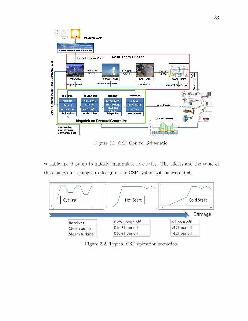
Figure 3.2 shows three scenarios: cycling, hot start and cold start. The MIMO
controller has access to the full state and can handle all functions of it, and explicitly
take into account in the control objectives, the time derivatives of metal temperature
and uniformity of temperature. There are several control inputs, such as molten salt
flow rate, molten salt input and output temperatures, steam and load conditions at
the turbine generators, flow rate from the thermal storage system, aiming of heliostats
that can be manipulated. Besides it can take into account factors which can be de-
signed in, such as responsive drive systems to quickly manipulate tracking and aiming
of few designated heliostats, a molten salt recirculation flow around the receiver, trim
33
Figure 3.1. CSP Control Schematic.
variable speed pump to quickly manipulate flow rates. The effects and the value of
these suggested changes in design of the CSP system will be evaluated.
Figure 3.2. Typical CSP operation scenarios.

34
3.4 Controller Development
Our development is motivated by the structure of the model we have developed.
We describe some of the non-standard steps needed to use well established linear
control design methods for our purposes. These steps are needed for both estimation
and control given the nonlinear dynamics of the power tower. The coupled equations
that model heat transfer to each pipe segment in the power tower and the transfer of
that energy to the high temperature fluid have a block strict-feedback structure, in
that nonlinearities in the dynamics are accessible through a single integrator.
• State Estimation: We typically have measurements of flow temperature and
can easily insert temperature sensors into the flow heads so each end of a tube
in the power tower has a temperature measurement. The block strict feedback
structure coupled with direct measurement of isolation, and flow rates permits
design of state estimators similar to Kreisselmeier K-filters [47] or Marino-Tomei
M-T filters [48] to estimate all temperature states.
• Parameter Estimation: The same parameterization used for the estimator above
is also used for system identification via least squares techniques, of various
physical parameters in the system that may differ from theoretical values and
vary from time to time depending upon operating conditions and age of the
plant. Our parameter estimation will run in batch mode so as to the lack of
convergence guarantees arising from standard adaptive control methods [49].
• Block Feedback Linearization for cancelling nonlinearities: Radiation heat losses
from the power tower tubes are strongly nonlinear; convection losses are also
nonlinear. Because of the block strict feedback structure, we can directly cancel
these nonlinearities [50], so that the system behaves linearly at any operating
condition, and the rates of temperature change in the metal follow linear dy-
namics.

35
• Model Reference Control: We choose reference models with dynamics that op-
timize our cost functions over a period of time and drive the dynamics of the
plant to these reference dynamics with our control inputssmall angular changes
of the heliostats, pumping rates, and perhaps some valves.
• Set point adaptation: Because of uncertainties in the models we use, and due
to changes in operating conditions, the plant will not follow the exact reference
trajectory specified for it. To ameliorate these conditions, and send trajectory
tracking to zero over the short term, we will use extremum seeking [51] to
optimize the angle set-points to heliostats and temperature set points for fluid
to optimize longer term cost functions. Set point adaptation via extremum
seeking comes with exponential convergence guarantees, making it possible for
us to incorporate this seamlessly into the longer time frame optimization.
• Long horizon optimization: Our objective is to form a cost function that incor-
porates the costs of thermal cycling of the power tower, mechanical cycling of
the heliostats and pumps, along with the profits from the market over a one day
time frame. We will use models of local climate, cloud movement, cloud track-
ing, and insolation to develop the overall cost function. This optimization will
be performed through receding horizon methods using standard mathematical
programming techniques.
• Recommendations for plant sensor placement/design alterations: Based on the
performance of our controls on high fidelity simulation models, we will develop
specifications for placing sensors to maximize the speed of plant control sys-
tem response, and minimize its lifecycle costs. Design alterations such as the
placement of additional valves or pumps will also be suggested.
These controllers can be implemented in any of the vendor supplied target hard-
ware platforms. We expect to deliver functional software and demonstrate the con-
troller using simulation of CSP operating under various operating modes .

36
3.5 Actuation Analysis
Actuation analysis is another important part in control and optimization design of
concentrating solar plant. Actuators are devices which transform an electrical input
signal into mechanical action or motion. Electrical motors, hydraulic pumps, relays
are examples of actuators. In concentrating systems, possible actuators that might
be used are electric motors with screw systems for heliostat position control and
hydraulic pumps for molten salt fluid and steam fluid rate control. The specification
of interest in our actuator selection includes:
• Electric motors
– Speed range.
– Accuracy.
– Torque dynamic response.
– Rated power.
– Efficiency.
– Load profile.
• Hydraulic pumps
– Operating speed.
– Operating temperature.
– Operating horsepower
– Maximum operating pressure.
– Continuous operating pressure.
– Maximum fluid viscosity.
– Maximum fluid flow Displacement per revolution.
– Speed-load characteristic equations.
37
A detailed comparison of electric motors and pumps are available in the appendix,
the research objective is to build up input-output relationship between of actuators,
especially the load profiles, which, will serve as constrains in final optimization func-
tions.
Affect control time scale, affect the equilibrium mapping
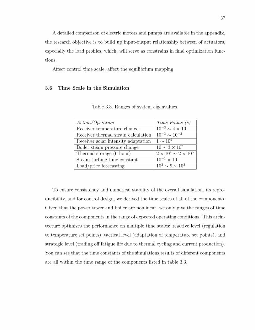
3.6 Time Scale in the Simulation
Table 3.3. Ranges of system eigenvalues.
Action/Operation Time Frame (s)Receiver temperature change 10−3 ∼ 4× 10Receiver thermal strain calculation 10−3 ∼ 10−2
Receiver solar intensity adaptation 1 ∼ 102
Boiler steam pressure change 10 ∼ 3× 10²
Thermal storage (6 hour) 2× 10⁴ ∼ 2× 10⁵
Steam turbine time constant 10−1 × 10Load/price forecasting 102 ∼ 9× 10²
To ensure consistency and numerical stability of the overall simulation, its repro-
ducibility, and for control design, we derived the time scales of all of the components.
Given that the power tower and boiler are nonlinear, we only give the ranges of time
constants of the components in the range of expected operating conditions. This archi-
tecture optimizes the performance on multiple time scales: reactive level (regulation
to temperature set points), tactical level (adaptation of temperature set points), and
strategic level (trading off fatigue life due to thermal cycling and current production).
You can see that the time constants of the simulations results of different components
are all within the time range of the components listed in table 3.3.
38
0.5
1
1.5
30
210
60
240
90
270
120
300
150
330
180 0
Figure 3.3. Optimized heliostat field position.
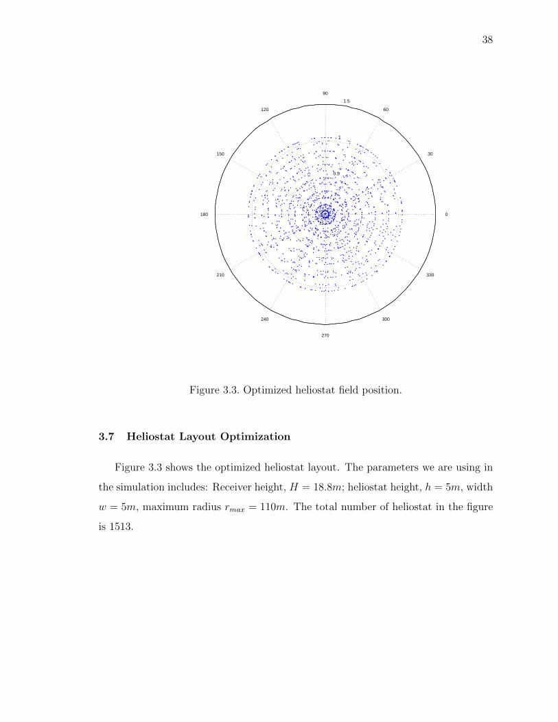
3.7 Heliostat Layout Optimization
Figure 3.3 shows the optimized heliostat layout. The parameters we are using in
the simulation includes: Receiver height, H = 18.8m; heliostat height, h = 5m, width
w = 5m, maximum radius rmax = 110m. The total number of heliostat in the figure
is 1513.
39
3.8 Solar Tower Thermal Dynamics with LQR Control
In this section, we develop a control algorithm for a linearised model around
equilibrium operation point, and build up tube life cycle - HTF flow rate relationship
around the equilibrium point.
We design our output electricity power for the CSP system to be 100MWe, the
calculated thermal power needed for this system would be 566.22MWt based on Sys-
tem Advisor Model (SAM) provided by National Renewable Energy Laboratory [52].
Based on the thermal power needed, the receiver tower dimensions we choose are:
Receiver height H = 18.8m, receiver diameter D = 15.11m, No. of headers N = 16
(8 headers on each of west & east side), with 4 panels/header and 18 tubes/panel.
The tube dimensions are: tube outside diameter Dtube = 0.04m, tube thickness
ttube = 0.00125m. Other parameters in this test case includes HTF properties: HTF
density ρHTF = 1739kg/m3, specific heat capacity CP,HTF = 1529J/kg/K, tube
density ρtube = 6400kg/m3 and tube specific heat capacity CP,tube = 500J/kg/K.
Maximum flow rate on each side mHTF = 581.74kg/s.
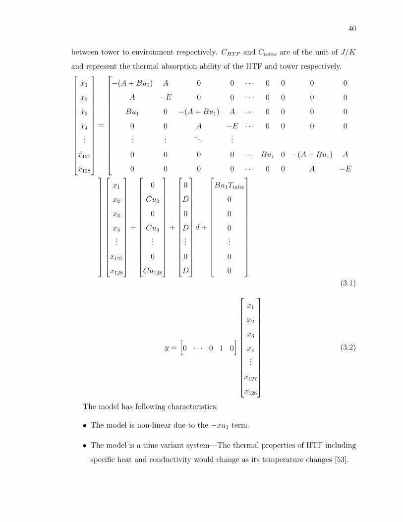
We take the east side of the tower in our analysis, and divide the thermal map into
8 × 8 nodes with energy balance analysis of each node shown as in figure 2.5. If we
denote x1, x3, ..., x127 to be the HTF temperature of the 8×8 nodes, and x2, x4, ..., x128
to be the tube temperature of the 8× 8 nodes, Equation (2.11) and Equation (2.12)
can be rewritten in matrix form as in Equation (3.1) and Equation (3.2).
In these two equations, we have notations A ∼ E defined as A = htubes−HTF ∗Atubes
CHTF,
B =CP,HTF
CHTF, C = 1
Ctubes, D = htubes−env∗Atubes
Ctubes, E = A+D. u1 is the control input 1 to
the system representing the header flow rate in unit of kg/s, u2 is the control input
2 to the system representing solar irradiation reflected by heliostats to each node in
unit of W , d is the disturbance to the system representing ambient temperature in
the unit of K. The subscript tubes represents the 72 tubes in the node of our interest,
Atubes is the surface area of the 72 tubes within one node. htubes−HTF and htubes−env
is the heat transfer coefficient between tower and HTF, and heat transfer coefficient
40
between tower to environment respectively. CHTF and Ctubes are of the unit of J/K
and represent the thermal absorption ability of the HTF and tower respectively.
x1
x2
x3
x4...
x127
x128
=
−(A+Bu1) A 0 0 · · · 0 0 0 0
A −E 0 0 · · · 0 0 0 0
Bu1 0 −(A+Bu1) A · · · 0 0 0 0
0 0 A −E · · · 0 0 0 0...
.... . .
...
0 0 0 0 · · · Bu1 0 −(A+Bu1) A
0 0 0 0 · · · 0 0 A −E
x1
x2
x3
x4...
x127
x128
+
0
Cu2
0
Cu4...
0
Cu128
+
0
D
0
D...
0
D
d+
Bu1Tinlet
0
0
0...
0
0
(3.1)
(3.2)y =[0 · · · 0 1 0
]
x1
x2
x3
x4...
x127
x128
The model has following characteristics:
• The model is non-linear due to the −xu1 term.
• The model is a time variant system—The thermal properties of HTF including
specific heat and conductivity would change as its temperature changes [53].
41
• The control input is limited: u1 needs to be in the range of 0 to 586kg/s, and
u2 needs to be in the range of 0 to Imax as well.
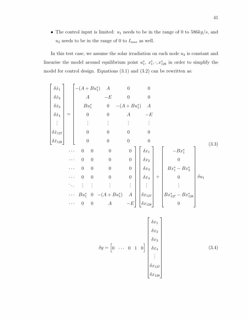
In this test case, we assume the solar irradiation on each node u2 is constant and
linearise the model around equilibrium point u∗1, x∗1, ·, x∗128 in order to simplify the
model for control design. Equations (3.1) and (3.2) can be rewritten as:
(3.3)
δx1
δx2
δx3
δx4...
δx127
δx128
=
−(A+Bu∗1) A 0 0
A −E 0 0
Bu∗1 0 −(A+Bu∗1) A
0 0 A −E...
......
...
0 0 0 0
0 0 0 0
· · · 0 0 0 0
· · · 0 0 0 0
· · · 0 0 0 0
· · · 0 0 0 0. . .
......
......
· · · Bu∗1 0 −(A+Bu∗1) A
· · · 0 0 A −E
δx1
δx2
δx3
δx4...
δx127
δx128
+
−Bx∗10
Bx∗1 −Bx∗30...
Bx∗127 −Bx∗1280
δu1
(3.4)δy =[0 · · · 0 1 0
]
δx1
δx2
δx3
δx4...
δx127
δx128
42
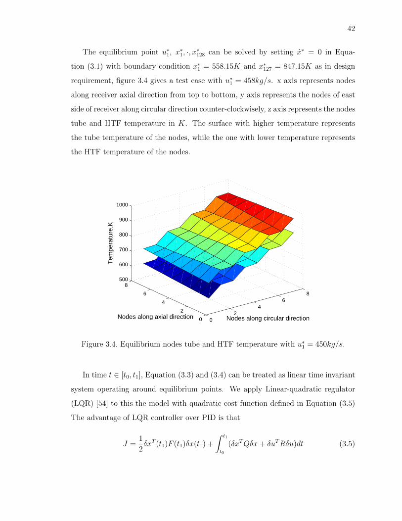
The equilibrium point u∗1, x∗1, ·, x∗128 can be solved by setting x∗ = 0 in Equa-
tion (3.1) with boundary condition x∗1 = 558.15K and x∗127 = 847.15K as in design
requirement, figure 3.4 gives a test case with u∗1 = 458kg/s. x axis represents nodes
along receiver axial direction from top to bottom, y axis represents the nodes of east
side of receiver along circular direction counter-clockwisely, z axis represents the nodes
tube and HTF temperature in K. The surface with higher temperature represents
the tube temperature of the nodes, while the one with lower temperature represents
the HTF temperature of the nodes.
02
46
8
0
2
4
6
8500
600
700
800
900
1000
Nodes along circular directionNodes along axial direction
Tem
pera
ture
,K
Figure 3.4. Equilibrium nodes tube and HTF temperature with u∗1 = 450kg/s.
In time t ∈ [t0, t1], Equation (3.3) and (3.4) can be treated as linear time invariant
system operating around equilibrium points. We apply Linear-quadratic regulator
(LQR) [54] to this the model with quadratic cost function defined in Equation (3.5)
The advantage of LQR controller over PID is that
J =1
2δxT (t1)F (t1)δx(t1) +
∫ t1
t0
(δxTQδx+ δuTRδu)dt (3.5)
43
with control law δu = −Kδx and initial condition δx(t0) = δx∗. K = [k1, k2, ..., k128]
is the LQR gain. Here if we assume the temperatures of all nodes are observable,
Equations above can be easily solved using standard numerical methods [55]. This
assumption is valid since we can directly measure the temperatures of different nodes
with a thermal camera.
0 20 40 60 80 100 120845
850
855
860
Time,s
Tem
pera
ture
, K
Reference HTF outlet temperatureActual HTF outlet temperature
0 20 40 60 80 100 120−15
−10
−5
0
Time,s
Con
trol
ler
outp
ut δ
u, k
g/s
Controller output
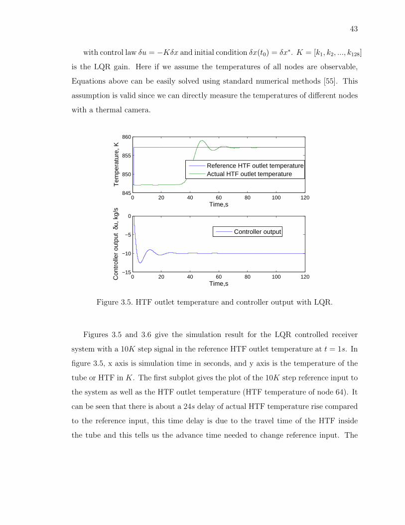
Figure 3.5. HTF outlet temperature and controller output with LQR.
Figures 3.5 and 3.6 give the simulation result for the LQR controlled receiver
system with a 10K step signal in the reference HTF outlet temperature at t = 1s. In
figure 3.5, x axis is simulation time in seconds, and y axis is the temperature of the
tube or HTF in K. The first subplot gives the plot of the 10K step reference input to
the system as well as the HTF outlet temperature (HTF temperature of node 64). It
can be seen that there is about a 24s delay of actual HTF temperature rise compared
to the reference input, this time delay is due to the travel time of the HTF inside
the tube and this tells us the advance time needed to change reference input. The
44
0 20 40 60 80 100 120−400
−200
0
200
400
Time,s
Tem
pera
ture
diff
eren
ce, K
Tube temperature difference along inlet header
0 20 40 60 80 100 12025
30
35
40
Time,s
Tem
pera
ture
diff
eren
ce, K
Tube temperature difference along outlet header
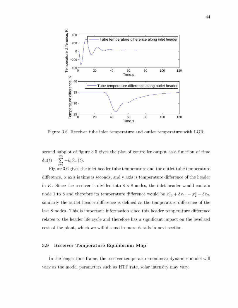
Figure 3.6. Receiver tube inlet temperature and outlet temperature with LQR.
second subplot of figure 3.5 gives the plot of controller output as a function of time
δu(t) =128∑i=1
−kiδxi(t).
Figure 3.6 gives the inlet header tube temperature and the outlet tube temperature
difference. x axis is time is seconds, and y axis is temperature difference of the header
in K. Since the receiver is divided into 8 × 8 nodes, the inlet header would contain
node 1 to 8 and therefore its temperature difference would be x∗16 + δx16 − x∗2 − δx2,
similarly the outlet header difference is defined as the temperature difference of the
last 8 nodes. This is important information since this header temperature difference
relates to the header life cycle and therefore has a significant impact on the levelized
cost of the plant, which we will discuss in more details in next section.
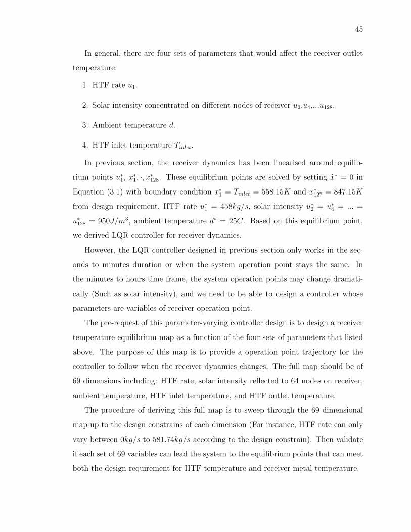
3.9 Receiver Temperature Equilibrium Map
In the longer time frame, the receiver temperature nonlinear dynamics model will
vary as the model parameters such as HTF rate, solar intensity may vary.
45
In general, there are four sets of parameters that would affect the receiver outlet
temperature:
1. HTF rate u1.
2. Solar intensity concentrated on different nodes of receiver u2,u4,...u128.
3. Ambient temperature d.
4. HTF inlet temperature Tinlet.
In previous section, the receiver dynamics has been linearised around equilib-
rium points u∗1, x∗1, ·, x∗128. These equilibrium points are solved by setting x∗ = 0 in
Equation (3.1) with boundary condition x∗1 = Tinlet = 558.15K and x∗127 = 847.15K
from design requirement, HTF rate u∗1 = 458kg/s, solar intensity u∗2 = u∗4 = ... =
u∗128 = 950J/m3, ambient temperature d∗ = 25C. Based on this equilibrium point,
we derived LQR controller for receiver dynamics.
However, the LQR controller designed in previous section only works in the sec-
onds to minutes duration or when the system operation point stays the same. In
the minutes to hours time frame, the system operation points may change dramati-
cally (Such as solar intensity), and we need to be able to design a controller whose
parameters are variables of receiver operation point.
The pre-request of this parameter-varying controller design is to design a receiver
temperature equilibrium map as a function of the four sets of parameters that listed
above. The purpose of this map is to provide a operation point trajectory for the
controller to follow when the receiver dynamics changes. The full map should be of
69 dimensions including: HTF rate, solar intensity reflected to 64 nodes on receiver,
ambient temperature, HTF inlet temperature, and HTF outlet temperature.
The procedure of deriving this full map is to sweep through the 69 dimensional
map up to the design constrains of each dimension (For instance, HTF rate can only
vary between 0kg/s to 581.74kg/s according to the design constrain). Then validate
if each set of 69 variables can lead the system to the equilibrium points that can meet
both the design requirement for HTF temperature and receiver metal temperature.

46
Here we use a simple 2D map to help illustrate this idea further more: We assume
HTF inlet temperature Tinlet = 558.15K, solar intensity u2 = u4 = ... = u128, ambient
temperature d∗ = 25C, target HTF output temperature at equilibrium is x∗127,target =
847.15K from design requirement. We then sweep the combination of HTF rate and
solar intensity on node (u1, u2) to find the receiver temperature equilibrium point.
The procedures are as follows:
1. Based on above constrains and receiver metal properties, derive the upper and
lower receiver tube temperature limit.
2. Derive the HTF and receiver tube temperature distribution along nodes based
on HTF inlet/outlet temperature equilibrium points and receiver tube temper-
ature limit.– This result will serve as the initial condition in solving the receiver
nonlinear dynamics equation.
3. Set x = 0 in Equation (3.1) and solve this non-linear equation using the trust-
region dogleg approach and initial conditions derived from previous step. HTF
inlet temperature Tinlet stays the same in the process.
4. Form a set of candidate combinations (u1, u2) as shown in figure 3.7 by checking
whether the HTF outlet temperature at equilibrium point is within the ±5K
of target HTF outlet temperature at equilibrium point x∗127,target.
5. Narrow down the candidate set by checking that: With the candidate combina-
tions (u1, u2), whether the receiver tube temperature exceeds its design limits
from step 1.
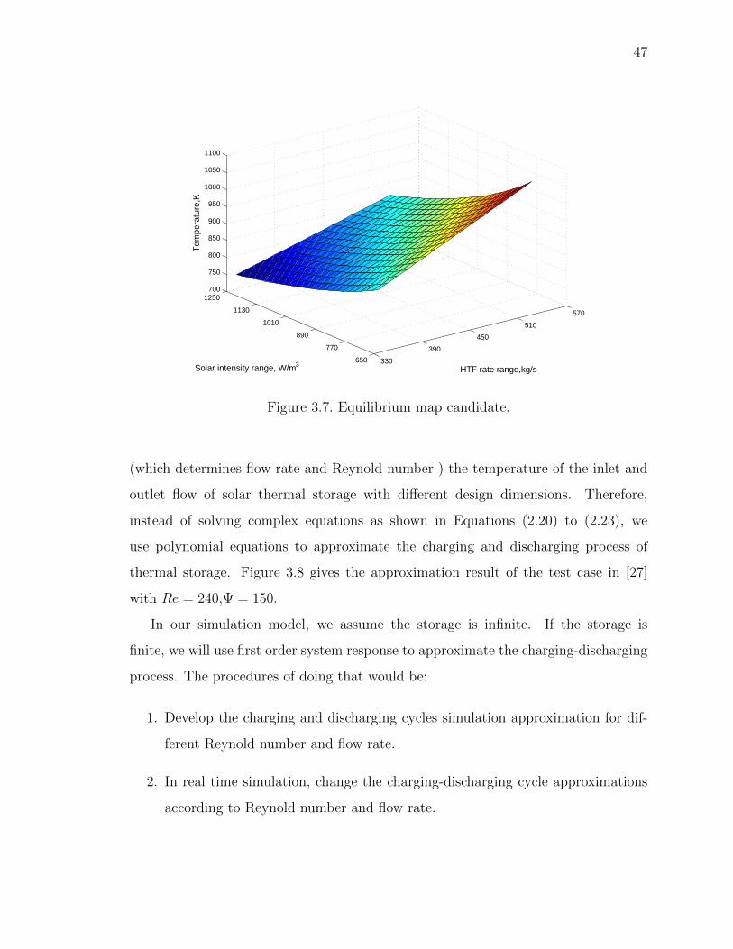
3.10 Heat Storage
The heat storage thermal dynamics is complex, therefore we created look-up tables
to describe the thermal dynamics during the charging-discharging process. From
control point of view, we are more interested in the relationship between pump rate
47
330
390
450
510
570
650
770
890
1010
1130
1250700
750
800
850
900
950
1000
1050
1100
HTF rate range,kg/s Solar intensity range, W/m3
Tem
pera
ture
,K
Figure 3.7. Equilibrium map candidate.
(which determines flow rate and Reynold number ) the temperature of the inlet and
outlet flow of solar thermal storage with different design dimensions. Therefore,
instead of solving complex equations as shown in Equations (2.20) to (2.23), we
use polynomial equations to approximate the charging and discharging process of
thermal storage. Figure 3.8 gives the approximation result of the test case in [27]
with Re = 240,Ψ = 150.
In our simulation model, we assume the storage is infinite. If the storage is
finite, we will use first order system response to approximate the charging-discharging
process. The procedures of doing that would be:
1. Develop the charging and discharging cycles simulation approximation for dif-
ferent Reynold number and flow rate.
2. In real time simulation, change the charging-discharging cycle approximations
according to Reynold number and flow rate.
48
0 0.5 1 1.50
0.1
0.2
0.3
0.4
0.5
0.6
0.7
0.8
0.9
1
Non−dimensional axial distance, X/C0
Non−dimensional temperature,
Θ
Discharge Charge
Figure 3.8. Discharge-charging cycle (Re = 240, Ψ = 150), H = 1.0C0, [27].
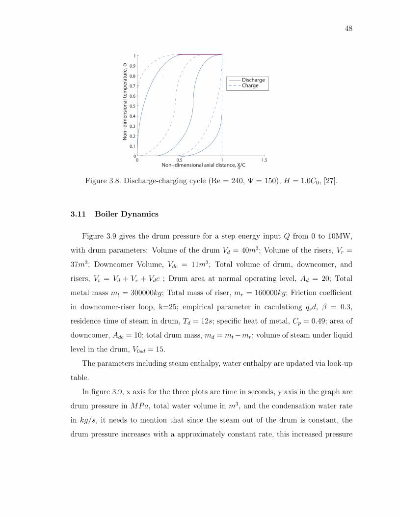
3.11 Boiler Dynamics
Figure 3.9 gives the drum pressure for a step energy input Q from 0 to 10MW,
with drum parameters: Volume of the drum Vd = 40m3; Volume of the risers, Vr =
37m3; Downcomer Volume, Vdc = 11m3; Total volume of drum, downcomer, and
risers, Vt = Vd + Vr + Vdc ; Drum area at normal operating level, Ad = 20; Total
metal mass mt = 300000kg; Total mass of riser, mr = 160000kg; Friction coefficient
in downcomer-riser loop, k=25; empirical parameter in caculationg qsd, β = 0.3,
residence time of steam in drum, Td = 12s; specific heat of metal, Cp = 0.49; area of
downcomer, Adc = 10; total drum mass, md = mt−mr; volume of steam under liquid
level in the drum, V0sd = 15.
The parameters including steam enthalpy, water enthalpy are updated via look-up
table.
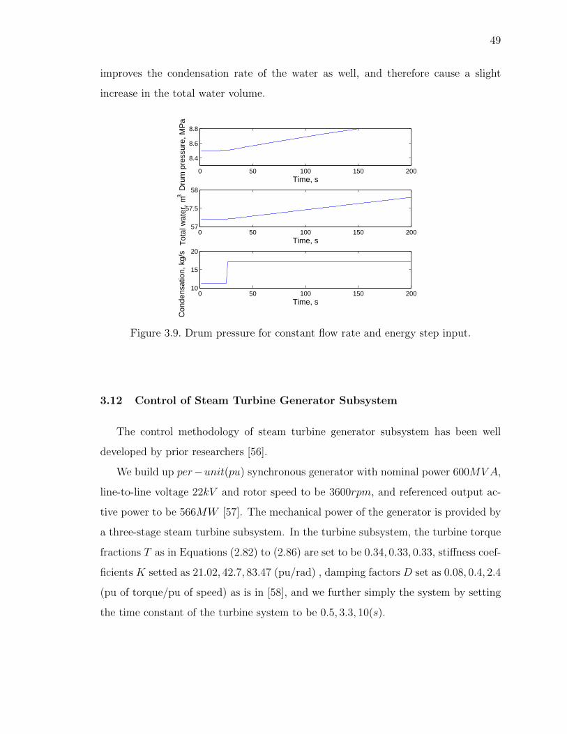
In figure 3.9, x axis for the three plots are time in seconds, y axis in the graph are
drum pressure in MPa, total water volume in m3, and the condensation water rate
in kg/s, it needs to mention that since the steam out of the drum is constant, the
drum pressure increases with a approximately constant rate, this increased pressure
49
improves the condensation rate of the water as well, and therefore cause a slight
increase in the total water volume.
0 50 100 150 200
8.4
8.6
8.8
Time, sD
rum
pre
ssur
e, M
Pa
0 50 100 150 20057
57.5
58
Time, sTot
al w
ater
, m3
0 50 100 150 20010
15
20
Time, s
Con
dens
atio
n, k
g/s
Figure 3.9. Drum pressure for constant flow rate and energy step input.
3.12 Control of Steam Turbine Generator Subsystem
The control methodology of steam turbine generator subsystem has been well
developed by prior researchers [56].
We build up per−unit(pu) synchronous generator with nominal power 600MVA,
line-to-line voltage 22kV and rotor speed to be 3600rpm, and referenced output ac-
tive power to be 566MW [57]. The mechanical power of the generator is provided by
a three-stage steam turbine subsystem. In the turbine subsystem, the turbine torque
fractions T as in Equations (2.82) to (2.86) are set to be 0.34, 0.33, 0.33, stiffness coef-
ficients K setted as 21.02, 42.7, 83.47 (pu/rad) , damping factors D set as 0.08, 0.4, 2.4
(pu of torque/pu of speed) as is in [58], and we further simply the system by setting
the time constant of the turbine system to be 0.5, 3.3, 10(s).
50
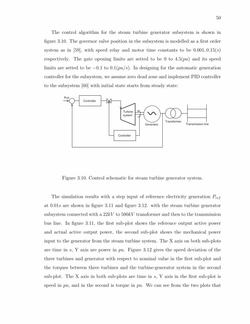
The control algorithm for the steam turbine generator subsystem is shown in
figure 3.10. The governor valve position in the subsystem is modelled as a first order
system as in [59], with speed relay and motor time constants to be 0.001, 0.15(s)
respectively. The gate opening limits are setted to be 0 to 4.5(pu) and its speed
limits are setted to be −0.1 to 0.1(pu/s). In designing for the automatic generation
controller for the subsystem, we assume zero dead zone and implement PID controller
to the subsystem [60] with initial state starts from steady state:
Turbine
system
ControllerPref
GeneratorTransformer
Transmission line
Controller
Figure 3.10. Control schematic for steam turbine generator system.
The simulation results with a step input of reference electricity generation Pref
at 0.01s are shown in figure 3.11 and figure 3.12. with the steam turbine generator
subsystem connected with a 22kV to 500kV transformer and then to the transmission
bus line. In figure 3.11, the first sub-plot shows the reference output active power
and actual active output power, the second sub-plot shows the mechanical power
input to the generator from the steam turbine system. The X axis on both sub-plots
are time in s, Y axis are power in pu. Figure 3.12 gives the speed deviation of the
three turbines and generator with respect to nominal value in the first sub-plot and
the torques between three turbines and the turbine-generator system in the second
sub-plot. The X axis in both sub-plots are time in s, Y axis in the first sub-plot is
speed in pu, and in the second is torque in pu. We can see from the two plots that
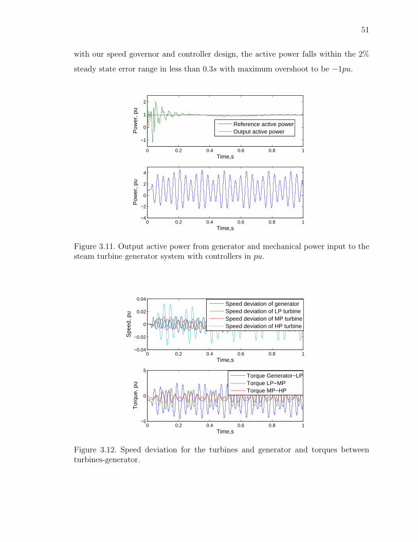
51
with our speed governor and controller design, the active power falls within the 2%
steady state error range in less than 0.3s with maximum overshoot to be −1pu.
0 0.2 0.4 0.6 0.8 1
−1
0
1
2
Time,s
Pow
er, p
u
Reference active powerOutput active power
0 0.2 0.4 0.6 0.8 1−4
−2
0
2
4
Time,s
Pow
er, p
u
Figure 3.11. Output active power from generator and mechanical power input to thesteam turbine generator system with controllers in pu.
0 0.2 0.4 0.6 0.8 1−0.04
−0.02
0
0.02
0.04
Time,s
Spe
ed, p
u
Speed deviation of generatorSpeed deviation of LP turbineSpeed deviation of MP turbineSpeed deviation of HP turbine
0 0.2 0.4 0.6 0.8 1−5
0
5
Time,s
Tor
que,
pu
Torque Generator−LPTorque LP−MPTorque MP−HP
Figure 3.12. Speed deviation for the turbines and generator and torques betweenturbines-generator.

52
4. CONTROLS WITH SMALL DISTURBANCE
4.1 Sensing and State Estimation
As stated in previous chapter, sensing and state estimation is essential in solar
concentrating plant optimization in order to have full state observability and control-
lability of whole system.
• Measurement and estimation of solar altitude angle αs and solar azimuth angle
γs and solar intensity I at time t and t+1 respectively.
• Measurement and estimation of tile angle Ψt, tile azimuth angle Psia, bias angle
of altitude axis from the orthogonal of azimuth axis τ1 and canting angle µ of the
altitude-azimuth tacking geometry of heliostats at time t and t+1 respectively.
• Measurement and estimation of ambient temperature Tamb, tube temperature
and HTF temperature Ttube(i, j, k), THTF (i, j, k) of the ith nodes on the jth
header of panel k in the receiver subsystem at time t and t+1 respectively.
• Measurement and estimation of axial temperature from hot molten salt temper-
ature Th to cold salt temperature Tl for both charging and discharging processes
at time t and t+1 respectively.
• Measurement and estimation of boiler input power Q, inlet volume and outlet
steam flow rate and steam temperature qf , qs, Tf , Ts, drum pressure pdrum, vol-
ume of steam under liquid level in the drum Vsd at time t and t+1 respectively.

53
• Measurement and estimation of the pressure in electricity generator pHP and
pLH in HP-turbine and in LP-turbine, as well as the steam temperature THP ,
TLP , steam flow rate qHP , qLP at time t and t+1 respectively.
• Measurement and estimation of electricity demands and prices in both day
ahead electricity markets and real time electricity markets DDA, DRT , pDA, pRT
at time t and t+1 respectively.
A general introduction of sensing technology in usage is in the appendix. In the
following objective, in each of the sensor we are going to use, the following characters
are needed for system design and :
• Input resolution.
• Output resolution.
• Input range.
• Output range.
• Maximum non-linearity.
• Maximum hysteresis.
• Reaction time.
4.2 Receiver Dynamics Model with Measurement Error and State Dis-
turbance
We are building a three-level controller architecture using multi-input-multi-output
(MIMO) control for CSP plants that can be implemented on existing plants to im-
prove performance, reliability, and extend the life of the plant as described in previous
sections. This architecture optimizes the performance on multiple time scales reactive
level (regulation to temperature set points), tactical level (adaptation of temperature
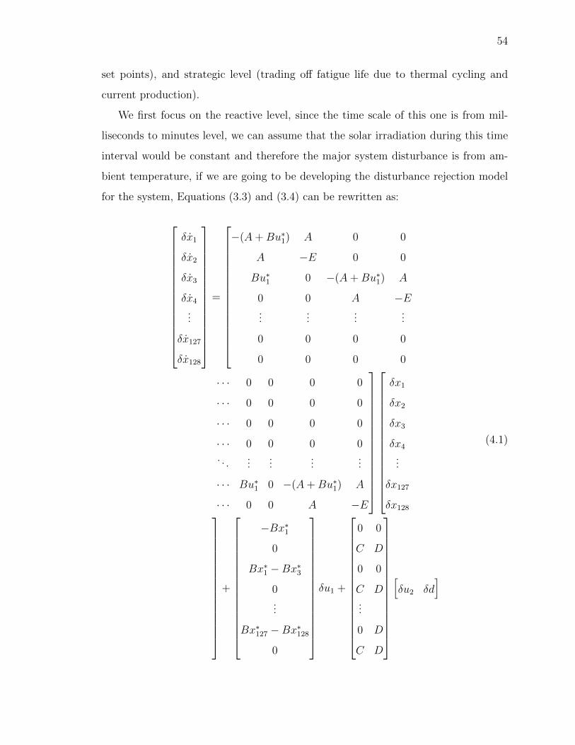
54
set points), and strategic level (trading off fatigue life due to thermal cycling and
current production).
We first focus on the reactive level, since the time scale of this one is from mil-
liseconds to minutes level, we can assume that the solar irradiation during this time
interval would be constant and therefore the major system disturbance is from am-
bient temperature, if we are going to be developing the disturbance rejection model
for the system, Equations (3.3) and (3.4) can be rewritten as:
(4.1)
δx1
δx2
δx3
δx4...
δx127
δx128
=
−(A+Bu∗1) A 0 0
A −E 0 0
Bu∗1 0 −(A+Bu∗1) A
0 0 A −E...
......
...
0 0 0 0
0 0 0 0
· · · 0 0 0 0
· · · 0 0 0 0
· · · 0 0 0 0
· · · 0 0 0 0. . .
......
......
· · · Bu∗1 0 −(A+Bu∗1) A
· · · 0 0 A −E
δx1
δx2
δx3
δx4...
δx127
δx128+
−Bx∗10
Bx∗1 −Bx∗30...
Bx∗127 −Bx∗1280
δu1 +
0 0
C D
0 0
C D...
0 D
C D
[δu2 δd
]
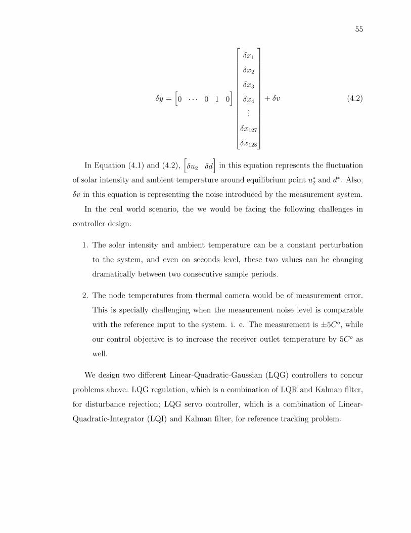
55
(4.2)δy =[0 · · · 0 1 0
]
δx1
δx2
δx3
δx4...
δx127
δx128
+ δv
In Equation (4.1) and (4.2),[δu2 δd
]in this equation represents the fluctuation
of solar intensity and ambient temperature around equilibrium point u∗2 and d∗. Also,
δv in this equation is representing the noise introduced by the measurement system.
In the real world scenario, the we would be facing the following challenges in
controller design:
1. The solar intensity and ambient temperature can be a constant perturbation
to the system, and even on seconds level, these two values can be changing
dramatically between two consecutive sample periods.
2. The node temperatures from thermal camera would be of measurement error.
This is specially challenging when the measurement noise level is comparable
with the reference input to the system. i. e. The measurement is ±5Co, while
our control objective is to increase the receiver outlet temperature by 5Co as
well.
We design two different Linear-Quadratic-Gaussian (LQG) controllers to concur
problems above: LQG regulation, which is a combination of LQR and Kalman filter,
for disturbance rejection; LQG servo controller, which is a combination of Linear-
Quadratic-Integrator (LQI) and Kalman filter, for reference tracking problem.
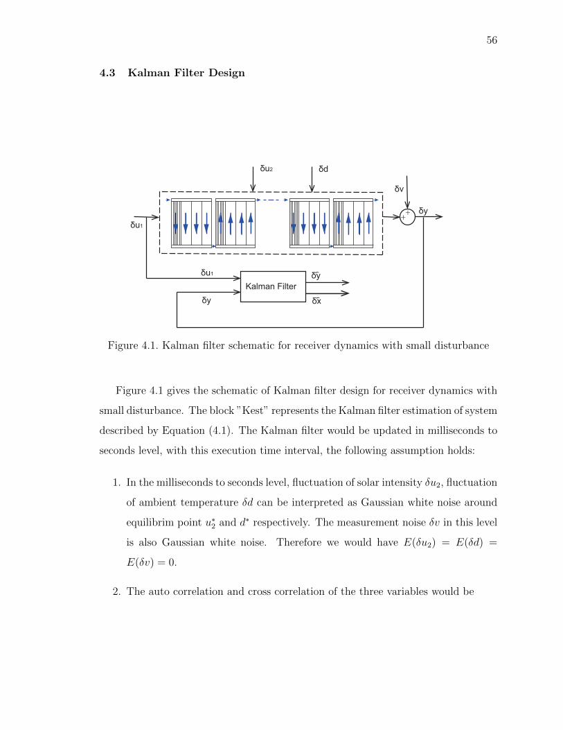
56
4.3 Kalman Filter Design
Kalman Filter
δu1
δx
δu1
δd δu2
δy
δy
++
δv
δy
Figure 4.1. Kalman filter schematic for receiver dynamics with small disturbance
Figure 4.1 gives the schematic of Kalman filter design for receiver dynamics with
small disturbance. The block ”Kest” represents the Kalman filter estimation of system
described by Equation (4.1). The Kalman filter would be updated in milliseconds to
seconds level, with this execution time interval, the following assumption holds:
1. In the milliseconds to seconds level, fluctuation of solar intensity δu2, fluctuation
of ambient temperature δd can be interpreted as Gaussian white noise around
equilibrim point u∗2 and d∗ respectively. The measurement noise δv in this level
is also Gaussian white noise. Therefore we would have E(δu2) = E(δd) =
E(δv) = 0.
2. The auto correlation and cross correlation of the three variables would be
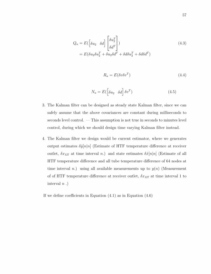
57
(4.3)Qn = E([δu2 δd
]δuT2δdT
)
= E(δu2δuT2 + δu2δd
T + δdδuT2 + δdδdT )
Rn = E(δvδvT ) (4.4)
(4.5)Nn = E([δu2 δd
]δvT )
3. The Kalman filter can be designed as steady state Kalman filter, since we can
safely assume that the above covariances are constant during milliseconds to
seconds level control. — This assumption is not true in seconds to minutes level
control, during which we should design time varying Kalman filter instead.
4. The Kalman filter we design would be current estimator, where we generates
output estimates δy[n|n] (Estimate of HTF temperature difference at receiver
outlet, δx127 at time interval n.) and state estimates δx[n|n] (Estimate of all
HTF temperature difference and all tube temperature difference of 64 nodes at
time interval n.) using all available measurements up to y(n) (Measurement
of of HTF temperature difference at receiver outlet, δx127 at time interval 1 to
interval n .)
If we define coefficients in Equation (4.1) as in Equation (4.6)
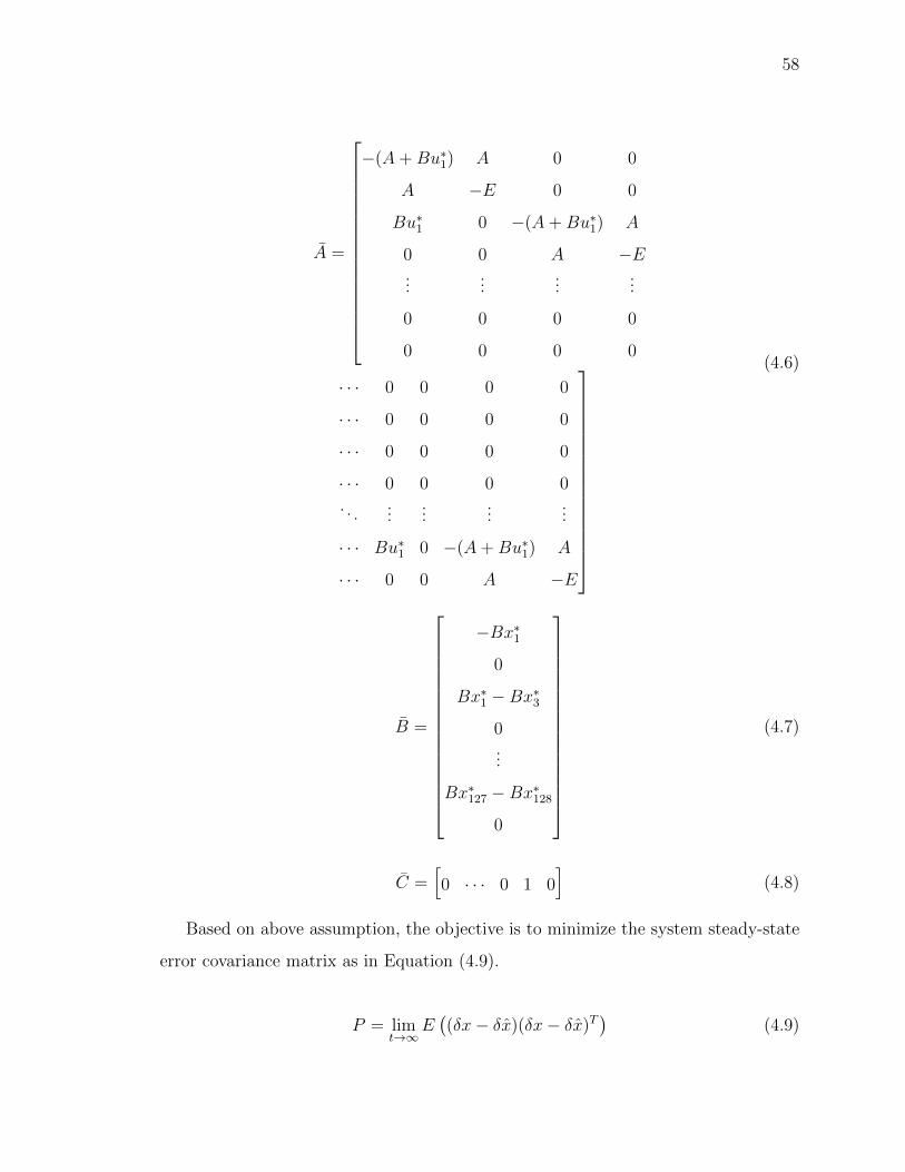
58
(4.6)
A =
−(A+Bu∗1) A 0 0
A −E 0 0
Bu∗1 0 −(A+Bu∗1) A
0 0 A −E...
......
...
0 0 0 0
0 0 0 0
· · · 0 0 0 0
· · · 0 0 0 0
· · · 0 0 0 0
· · · 0 0 0 0. . .
......
......
· · · Bu∗1 0 −(A+Bu∗1) A
· · · 0 0 A −E
B =
−Bx∗10
Bx∗1 −Bx∗30...
Bx∗127 −Bx∗1280
(4.7)
C =[0 · · · 0 1 0
](4.8)
Based on above assumption, the objective is to minimize the system steady-state
error covariance matrix as in Equation (4.9).
P = limt→∞
E((δx− δx)(δx− δx)T
)(4.9)
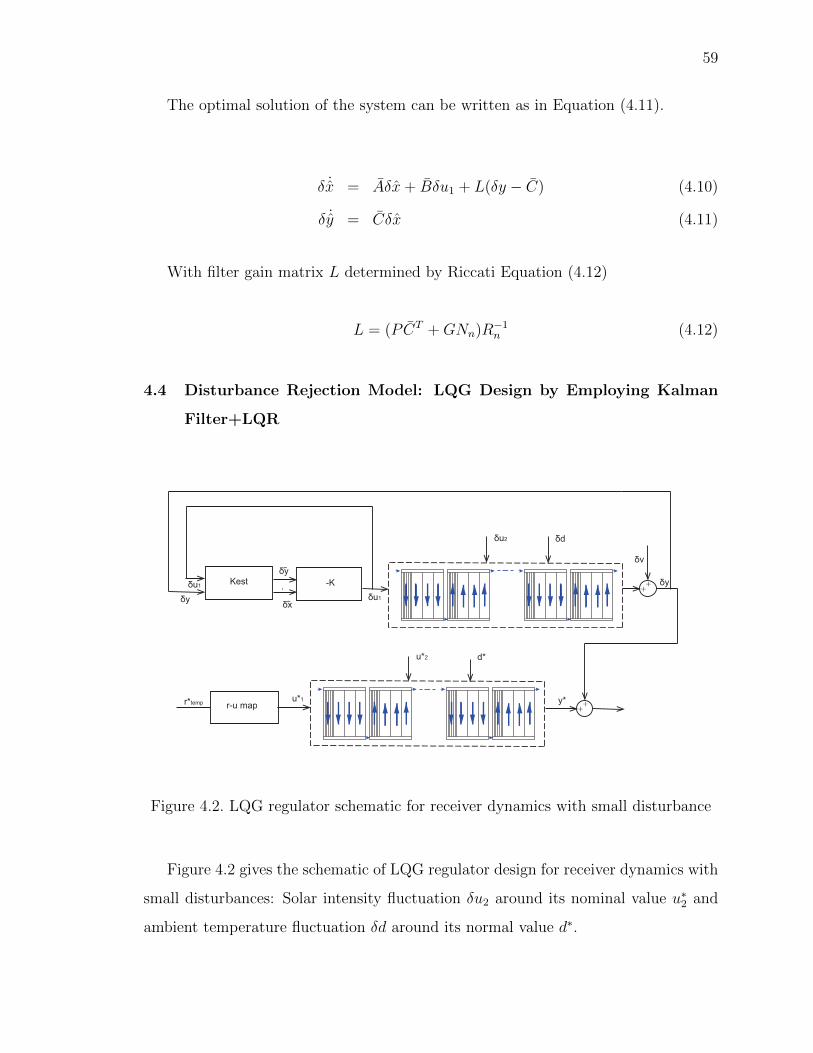
59
The optimal solution of the system can be written as in Equation (4.11).
δ ˙x = Aδx+ Bδu1 + L(δy − C) (4.10)
δ ˙y = Cδx (4.11)
With filter gain matrix L determined by Riccati Equation (4.12)
L = (PCT +GNn)R−1n (4.12)
4.4 Disturbance Rejection Model: LQG Design by Employing Kalman
Filter+LQR
Kest δu1
δx
r*temp
δu1
δd δu2
δy
u*1
d* u*2
y*
-K
r-u map
δy
++
++
δv
δy
Figure 4.2. LQG regulator schematic for receiver dynamics with small disturbance
Figure 4.2 gives the schematic of LQG regulator design for receiver dynamics with
small disturbances: Solar intensity fluctuation δu2 around its nominal value u∗2 and
ambient temperature fluctuation δd around its normal value d∗.
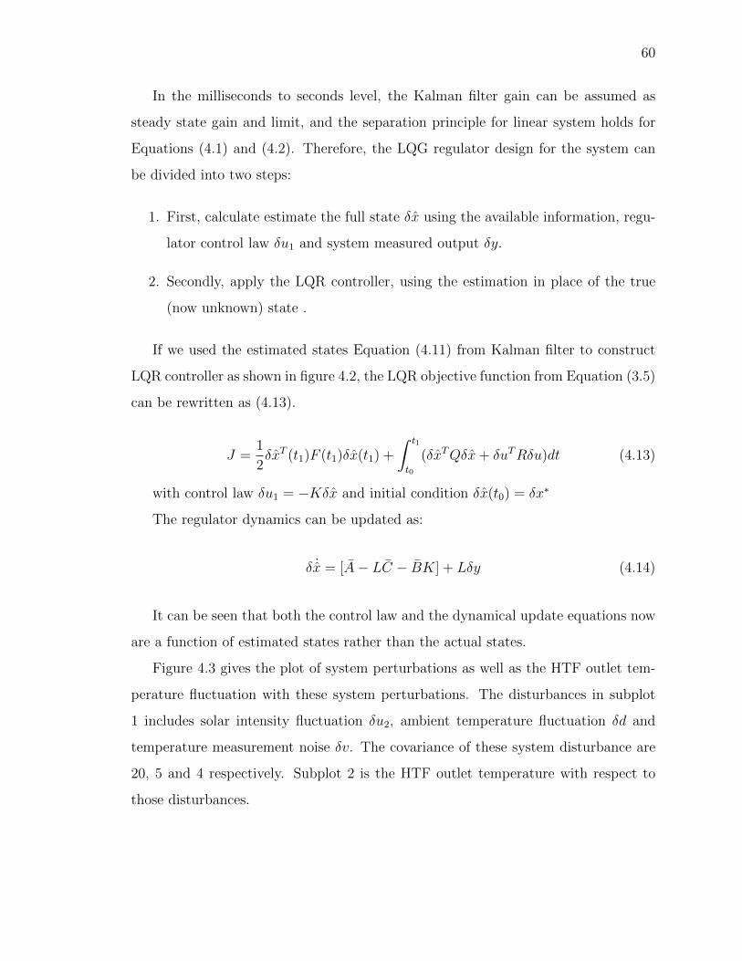
60
In the milliseconds to seconds level, the Kalman filter gain can be assumed as
steady state gain and limit, and the separation principle for linear system holds for
Equations (4.1) and (4.2). Therefore, the LQG regulator design for the system can
be divided into two steps:
1. First, calculate estimate the full state δx using the available information, regu-
lator control law δu1 and system measured output δy.
2. Secondly, apply the LQR controller, using the estimation in place of the true
(now unknown) state .
If we used the estimated states Equation (4.11) from Kalman filter to construct
LQR controller as shown in figure 4.2, the LQR objective function from Equation (3.5)
can be rewritten as (4.13).
J =1
2δxT (t1)F (t1)δx(t1) +
∫ t1
t0
(δxTQδx+ δuTRδu)dt (4.13)
with control law δu1 = −Kδx and initial condition δx(t0) = δx∗
The regulator dynamics can be updated as:
δ ˙x = [A− LC − BK] + Lδy (4.14)
It can be seen that both the control law and the dynamical update equations now
are a function of estimated states rather than the actual states.
Figure 4.3 gives the plot of system perturbations as well as the HTF outlet tem-
perature fluctuation with these system perturbations. The disturbances in subplot
1 includes solar intensity fluctuation δu2, ambient temperature fluctuation δd and
temperature measurement noise δv. The covariance of these system disturbance are
20, 5 and 4 respectively. Subplot 2 is the HTF outlet temperature with respect to
those disturbances.
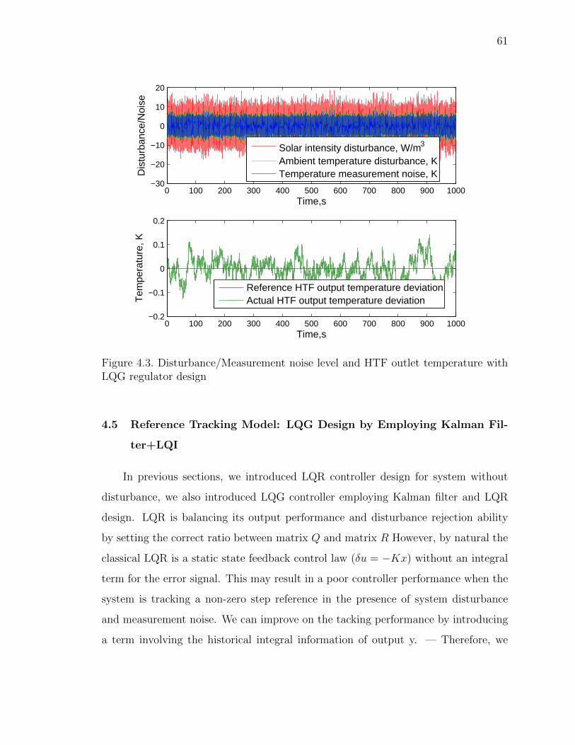
61
0 100 200 300 400 500 600 700 800 900 1000−30
−20
−10
0
10
20
Time,s
Dis
turb
ance
/Noi
se
Solar intensity disturbance, W/m3
Ambient temperature disturbance, KTemperature measurement noise, K
0 100 200 300 400 500 600 700 800 900 1000−0.2
−0.1
0
0.1
0.2
Time,s
Tem
pera
ture
, K
Reference HTF output temperature deviationActual HTF output temperature deviation
Figure 4.3. Disturbance/Measurement noise level and HTF outlet temperature withLQG regulator design
4.5 Reference Tracking Model: LQG Design by Employing Kalman Fil-
ter+LQI
In previous sections, we introduced LQR controller design for system without
disturbance, we also introduced LQG controller employing Kalman filter and LQR
design. LQR is balancing its output performance and disturbance rejection ability
by setting the correct ratio between matrix Q and matrix R However, by natural the
classical LQR is a static state feedback control law (δu = −Kx) without an integral
term for the error signal. This may result in a poor controller performance when the
system is tracking a non-zero step reference in the presence of system disturbance
and measurement noise. We can improve on the tacking performance by introducing
a term involving the historical integral information of output y. — Therefore, we
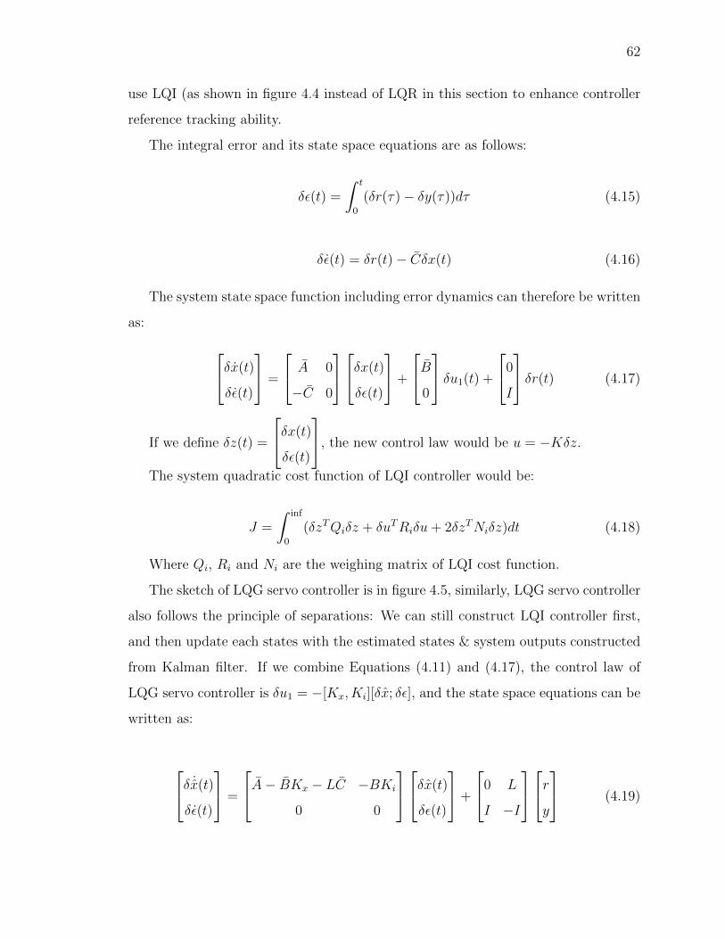
62
use LQI (as shown in figure 4.4 instead of LQR in this section to enhance controller
reference tracking ability.
The integral error and its state space equations are as follows:
δε(t) =
∫ t
0
(δr(τ)− δy(τ))dτ (4.15)
δε(t) = δr(t)− Cδx(t) (4.16)
The system state space function including error dynamics can therefore be written
as:
δx(t)
δε(t)
=
A 0
−C 0
δx(t)
δε(t)
+
B0
δu1(t) +
0
I
δr(t) (4.17)
If we define δz(t) =
δx(t)
δε(t)
, the new control law would be u = −Kδz.
The system quadratic cost function of LQI controller would be:
J =
∫ inf
0
(δzTQiδz + δuTRiδu+ 2δzTNiδz)dt (4.18)
Where Qi, Ri and Ni are the weighing matrix of LQI cost function.
The sketch of LQG servo controller is in figure 4.5, similarly, LQG servo controller
also follows the principle of separations: We can still construct LQI controller first,
and then update each states with the estimated states & system outputs constructed
from Kalman filter. If we combine Equations (4.11) and (4.17), the control law of
LQG servo controller is δu1 = −[Kx, Ki][δx; δε], and the state space equations can be
written as:
δ ˙x(t)
δε(t)
=
A− BKx − LC −BKi
0 0
δx(t)
δε(t)
+
0 L
I −I
ry
(4.19)
63
Integrator
δrtemp
r*temp
δu1
δy
u*1
d* u*2
y*
K
r-u map
+-
++
δx
Figure 4.4. LQI controller schematic for receiver dynamics with small disturbance
Integrator
δrtemp
Kest δu1
δx
r*temp
δu1
δd δu2
δy
u*1
d* u*2
y*
K
r-u map
δy
+-
++
++
δv
Figure 4.5. LQG reference controller schematic for receiver dynamics with small dis-turbance
Figure 4.5 gives a controller design for receiver dynamics with small disturbance.
The disturbances in subplot 1 includes solar intensity fluctuation δu2, ambient tem-
perature fluctuation δd and temperature measurement noise δv. The covariance of
these system disturbance are 20,5 and 4 respectively. Subplot 2 is the step increase
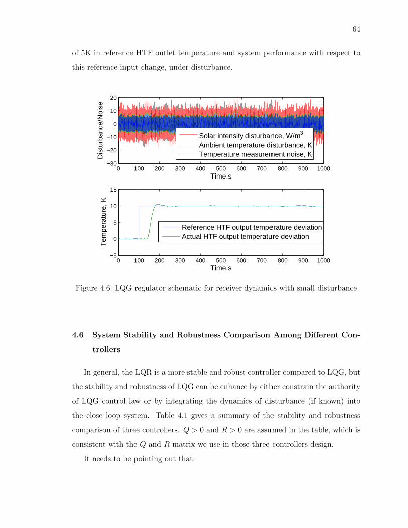
64
of 5K in reference HTF outlet temperature and system performance with respect to
this reference input change, under disturbance.
0 100 200 300 400 500 600 700 800 900 1000−30
−20
−10
0
10
20
Time,s
Dis
turb
ance
/Noi
se
Solar intensity disturbance, W/m3
Ambient temperature disturbance, KTemperature measurement noise, K
0 100 200 300 400 500 600 700 800 900 1000−5
0
5
10
15
Time,s
Tem
pera
ture
, K
Reference HTF output temperature deviationActual HTF output temperature deviation
Figure 4.6. LQG regulator schematic for receiver dynamics with small disturbance
4.6 System Stability and Robustness Comparison Among Different Con-
trollers
In general, the LQR is a more stable and robust controller compared to LQG, but
the stability and robustness of LQG can be enhance by either constrain the authority
of LQG control law or by integrating the dynamics of disturbance (if known) into
the close loop system. Table 4.1 gives a summary of the stability and robustness
comparison of three controllers. Q > 0 and R > 0 are assumed in the table, which is
consistent with the Q and R matrix we use in those three controllers design.
It needs to be pointing out that:

65
Table 4.1. Controller stability and robustness comparison
- Stability RobustnessLQR Asymptotically stable Gain margin inf, phase mar-
gin 60o [61]LQG regulator Conditionally stable Not guaranteed, can be im-
provedLQG servo controller Conditionally stable Not guaranteed, can be im-
proved
1. The stability of the LQG is conditional.
LQG is considered as asymptotic stable only when the we have perfect knowl-
edge of system parameters. This means the coefficients of state estimator from
Equation (4.11) and the coefficients of LQR/LQI dynamics as in Equation (4.17)
should be stable. i.e. Aestimator = Acontroller, Bestimator = Bcontroller ..., which is
the case in our previous controllers design. In this case,
(a) Estimator error affects state response.
(b) Actual states do not affect error propagation.
(c) System disturbance and measurement noise affect the estimator error and
actual states equally.
The system is therefore stable since all the sub-matrix of the state coefficients
in Equation (4.17) are stable.
2. The robustness of LQG is not guaranteed, but can be improved.
If the system parameters are uncertain, i.e. Aestimator 6= Acontroller, Bestimator 6=
Bcontroller ..., the close loop system and estimator response are coupled and
uncertainty parameters affect the close loop system eigenvalues. The detailed
derivation of equations has been illustrated as in [62] and [63].
LQR with loop transfer recovery (LQG/LTR) is commonly used solution to
enhance the robustness of LQG [64] [65]. The general idea is to reduce the

66
system sensitivity function by increasing the system process noise [66]. The
pre-requests for LQR/LTR [67] are
(a) Number of open loop system input (δu1) is equal to system output (δy).
(b) Plant (receiver dynamics) has no unstable zero.
Our plant model meets both requirements, making LQG/LTR a good candidate
for improving the system robustness.
Other methods includes the H∞ controller design, which assumes the worst
possible perturbation to the plant at all time in the process of controller de-
sign [68]; and design of disturbance based filter if the disturbance dynamics can
be well defined.
But in all the methods mentioned above, the enhancement of system robustness
is at the sacrifice of controller performance.
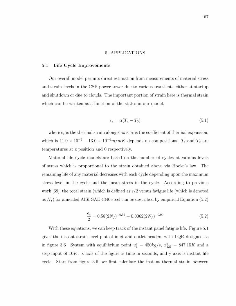
67
5. APPLICATIONS
5.1 Life Cycle Improvements
Our overall model permits direct estimation from measurements of material stress
and strain levels in the CSP power tower due to various transients–either at startup
and shutdown or due to clouds. The important portion of strain here is thermal strain
which can be written as a function of the states in our model.
εz = α(Tz − T0) (5.1)
where εz is the thermal strain along z axis, α is the coefficient of thermal expansion,
which is 11.0 × 10⁻⁶ − 13.0 × 10⁻⁶m/mK depends on compositions. Tz and T0 are
temperatures at z position and 0 respectively.
Material life cycle models are based on the number of cycles at various levels
of stress which is proportional to the strain obtained above via Hooke’s law. The
remaining life of any material decreases with each cycle depending upon the maximum
stress level in the cycle and the mean stress in the cycle. According to previous
work [69], the total strain (which is defined as ε/2 versus fatigue life (which is denoted
as Nf ) for annealed AISI-SAE 4340 steel can be described by empirical Equation (5.2)
εz2
= 0.58(2Nf )−0.57 + 0.0062(2Nf )
−0.09 (5.2)
With these equations, we can keep track of the instant panel fatigue life. Figure 5.1
gives the instant strain level plot of inlet and outlet headers with LQR designed as
in figure 3.6—System with equilibrium point u∗1 = 450kg/s, x∗127 = 847.15K and a
step-input of 10K. x axis of the figure is time in seconds, and y axis is instant life
cycle. Start from figure 3.6, we first calculate the instant thermal strain between
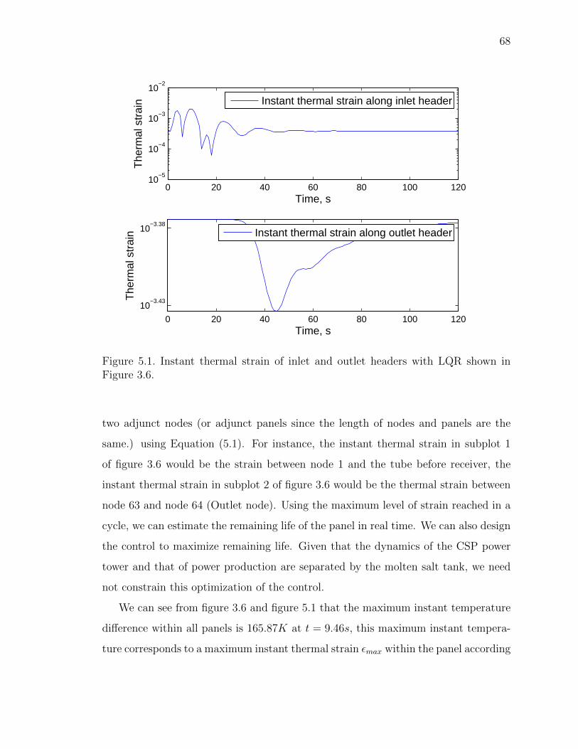
68
0 20 40 60 80 100 12010
−5
10−4
10−3
10−2
Time, s
The
rmal
str
ain
Instant thermal strain along inlet header
0 20 40 60 80 100 120
10−3.43
10−3.38
Time, s
The
rmal
str
ain
Instant thermal strain along outlet header
Figure 5.1. Instant thermal strain of inlet and outlet headers with LQR shown inFigure 3.6.
two adjunct nodes (or adjunct panels since the length of nodes and panels are the
same.) using Equation (5.1). For instance, the instant thermal strain in subplot 1
of figure 3.6 would be the strain between node 1 and the tube before receiver, the
instant thermal strain in subplot 2 of figure 3.6 would be the thermal strain between
node 63 and node 64 (Outlet node). Using the maximum level of strain reached in a
cycle, we can estimate the remaining life of the panel in real time. We can also design
the control to maximize remaining life. Given that the dynamics of the CSP power
tower and that of power production are separated by the molten salt tank, we need
not constrain this optimization of the control.
We can see from figure 3.6 and figure 5.1 that the maximum instant temperature
difference within all panels is 165.87K at t = 9.46s, this maximum instant tempera-
ture corresponds to a maximum instant thermal strain εmax within the panel according
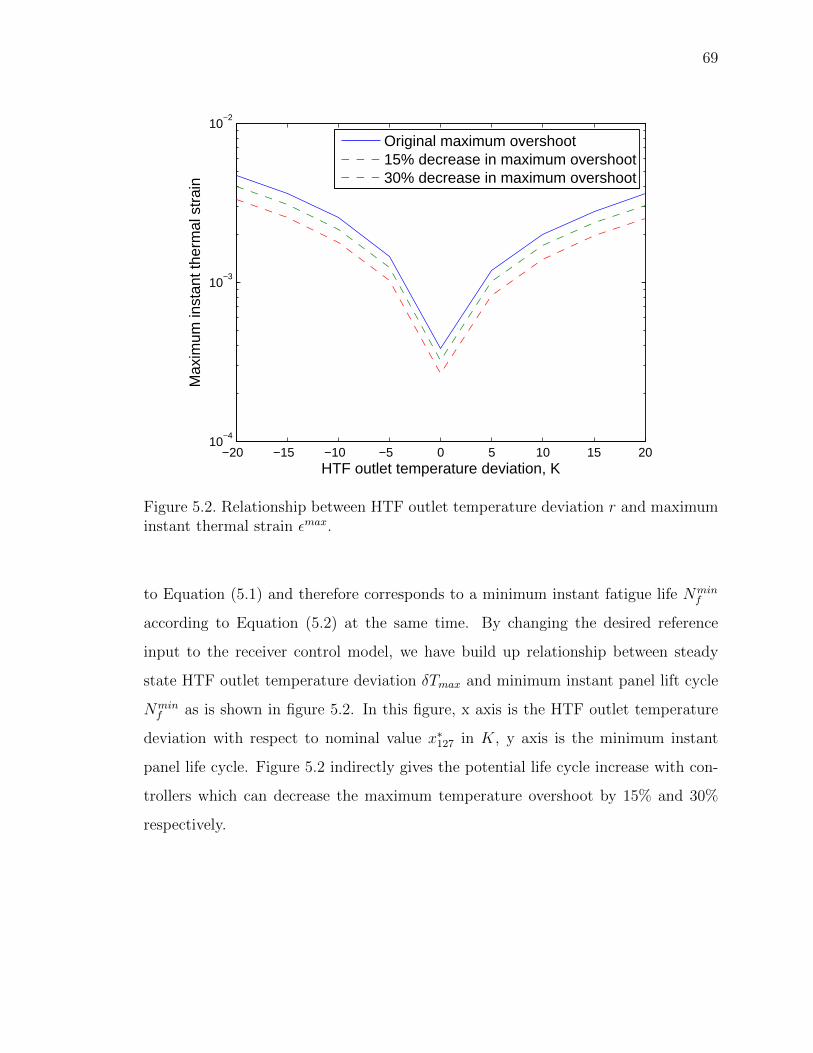
69
−20 −15 −10 −5 0 5 10 15 2010
−4
10−3
10−2
HTF outlet temperature deviation, K
Max
imum
inst
ant t
herm
al s
trai
n
Original maximum overshoot15% decrease in maximum overshoot30% decrease in maximum overshoot
Figure 5.2. Relationship between HTF outlet temperature deviation r and maximuminstant thermal strain εmax.
to Equation (5.1) and therefore corresponds to a minimum instant fatigue life Nminf
according to Equation (5.2) at the same time. By changing the desired reference
input to the receiver control model, we have build up relationship between steady
state HTF outlet temperature deviation δTmax and minimum instant panel lift cycle
Nminf as is shown in figure 5.2. In this figure, x axis is the HTF outlet temperature
deviation with respect to nominal value x∗127 in K, y axis is the minimum instant
panel life cycle. Figure 5.2 indirectly gives the potential life cycle increase with con-
trollers which can decrease the maximum temperature overshoot by 15% and 30%
respectively.
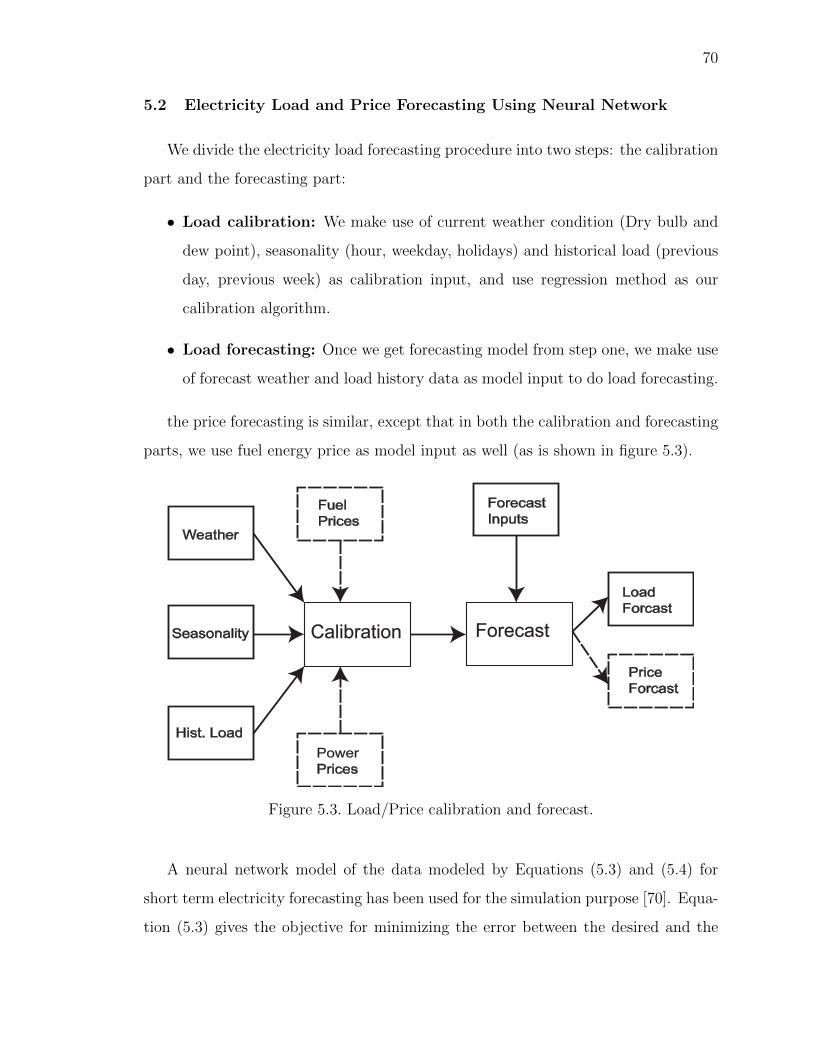
70
5.2 Electricity Load and Price Forecasting Using Neural Network
We divide the electricity load forecasting procedure into two steps: the calibration
part and the forecasting part:
• Load calibration: We make use of current weather condition (Dry bulb and
dew point), seasonality (hour, weekday, holidays) and historical load (previous
day, previous week) as calibration input, and use regression method as our
calibration algorithm.
• Load forecasting: Once we get forecasting model from step one, we make use
of forecast weather and load history data as model input to do load forecasting.
the price forecasting is similar, except that in both the calibration and forecasting
parts, we use fuel energy price as model input as well (as is shown in figure 5.3).
Seasonality
Weather
Hist. Load
Fuel
Prices
Power
Prices
Forecast
Inputs
Calibration Forecast
Price
Forcast
Load
Forcast
Figure 5.3. Load/Price calibration and forecast.
A neural network model of the data modeled by Equations (5.3) and (5.4) for
short term electricity forecasting has been used for the simulation purpose [70]. Equa-
tion (5.3) gives the objective for minimizing the error between the desired and the
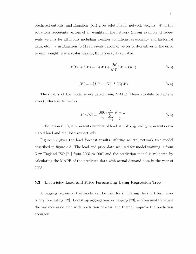
71
predicted outputs, and Equation (5.4) gives solutions for network weights. W in the
equations represents vectors of all weights in the network (In our example, it repre-
sents weights for all inputs including weather conditions, seasonality and historical
data, etc.). J in Equation (5.4) represents Jacobian vector of derivatives of the error
to each weight, µ is a scalar making Equation (5.4) solvable.
E(W + δW ) = E(W ) +∂E
∂WδW +O(n), (5.3)
δW = −[JJ t + µ[I]]−1JE(W ). (5.4)
The quality of the model is evaluated using MAPE (Mean absolute percentage
error), which is defined as
MAPE =100%
n
n∑t=1
| qt − qtqt|. (5.5)
In Equation (5.5), n represents number of load samples, qt and qt represents esti-
mated load and real load respectively.
Figure 5.4 gives the load forecast results utilizing neutral network tree model
described in figure 5.3. The load and price data we used for model training is from
New England ISO [71] from 2005 to 2007 and the prediction model is validated by
calculating the MAPE of the predicted data with actual demand data in the year of
2008.
5.3 Electricity Load and Price Forecasting Using Regression Tree
A bagging regression tree model can be used for simulating the short term elec-
tricity forecasting [72]. Bootstrap aggregation, or bagging [73], is often used to reduce
the variance associated with prediction process, and thereby improve the prediction
accuracy.
72
12/20/08 12/27/081
1.5
2
2.5x 10
6
Time, days
Ele
ctric
ity L
oad,
Wh
12/20/08 12/27 /08−4
−2
0
2x 10
5
MAPE: 2.41%
Time, daysEle
ctric
ity lo
ad d
iffer
ence
, Wh
ActualModel
Figure 5.4. Load forecast and MAPE evaluation for neural network prediction model(12/15/2008-12/29/2008).
The idea is simple: The bootstrap samples are drawn from the available electricity
load data, which has been pre-sorted according to weather, seasonality and historical
data. Then apply a set of regression trees each with a different set of rules for perform-
ing the non-linear regression. Next we combine the results by averaging for regression
and simple voting for classification. Following these steps we can finally obtain the
overall prediction, with reduced variance due to the averaging. The importance of
different predictors can be evaluated according to their out-of-bag estimates.
In the bagging process, roughly 37% of the original observations are left out as
out-of-bag observation. The quality of the prediction model can be evaluated using
out-of-bag error evaluation, which is defined as
73
εob =
∑ni=1M
−1N
∑Nk=1 f(·)|Xi,Yi /∈Sk |Yi − g∗k(Xi)|
2
n. (5.6)
where MN is defined as
MN =N∑i=1
f(·)|Xi,Yi /∈Sk (5.7)
In above equations, εob is the out-of-bag error for bagging regression tree, Sk is
the union of all estimators whose original sample indices got resampled in the kth
bootstrap sample. They other parameters in the above two equations are defined in
Appendix.
1. Create test matrix and target function for bagging
The influence factors in figure 5.3 and the electricity load history data would
be sorted into pairs (Xi, Yi, where i = 1, 2, 3..., n. Xi is the 7 dimensional
matrix including: weather condition (Dry bulb and dew point), seasonality
(hour, weekday, holidays) and historical load (previous day average ,same hour
previous day, same hour same day previous week previous week). Yi is the
electricity load. The system target function would be: E[Y |X = x].
2. Construct regression model estimators
If we define the estimator equation to be
g(·) = f (Xi, Yi)) (5.8)
The simplest estimator with only one split and two nodes would be,
g(X = x) = α1f(·)|x<d + α2f(·)|x≥d (5.9)
where we have α1, α2 and d defined as
(α1, α2, d) = argminα1,α2,d
i=n∑i=1
(Yi − α1f(·)|x<d − α2f(·)|x≥d) (5.10)
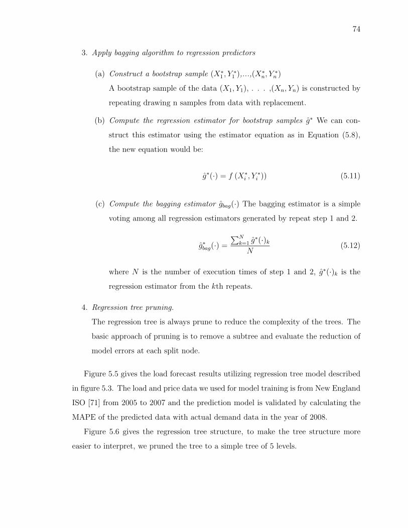
74
3. Apply bagging algorithm to regression predictors
(a) Construct a bootstrap sample (X∗1 , Y∗1 ),...,(X∗n, Y
∗n )
A bootstrap sample of the data (X1, Y1), . . . ,(Xn, Yn) is constructed by
repeating drawing n samples from data with replacement.
(b) Compute the regression estimator for bootstrap samples g∗ We can con-
struct this estimator using the estimator equation as in Equation (5.8),
the new equation would be:
g∗(·) = f (X∗i , Y∗i )) (5.11)
(c) Compute the bagging estimator gbag(·) The bagging estimator is a simple
voting among all regression estimators generated by repeat step 1 and 2.
g∗bag(·) =
∑Nk=1 g
∗(·)kN
(5.12)
where N is the number of execution times of step 1 and 2, g∗(·)k is the
regression estimator from the kth repeats.
4. Regression tree pruning.
The regression tree is always prune to reduce the complexity of the trees. The
basic approach of pruning is to remove a subtree and evaluate the reduction of
model errors at each split node.
Figure 5.5 gives the load forecast results utilizing regression tree model described
in figure 5.3. The load and price data we used for model training is from New England
ISO [71] from 2005 to 2007 and the prediction model is validated by calculating the
MAPE of the predicted data with actual demand data in the year of 2008.
Figure 5.6 gives the regression tree structure, to make the tree structure more
easier to interpret, we pruned the tree to a simple tree of 5 levels.
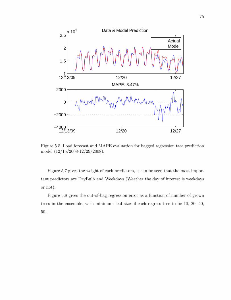
75
12/13/09 12/20 12/271
1.5
2
2.5x 10
4 Data & Model Prediction
12/13/09 12/20 12/27−4000
−2000
0
2000MAPE: 3.47%
ActualModel
Figure 5.5. Load forecast and MAPE evaluation for bagged regression tree predictionmodel (12/15/2008-12/29/2008).
Figure 5.7 gives the weight of each predictors, it can be seen that the most impor-
tant predictors are DryBulb and Weekdays (Weather the day of interest is weekdays
or not).
Figure 5.8 gives the out-of-bag regression error as a function of number of grown
trees in the ensemble, with minimum leaf size of each regress tree to be 10, 20, 40,
50.
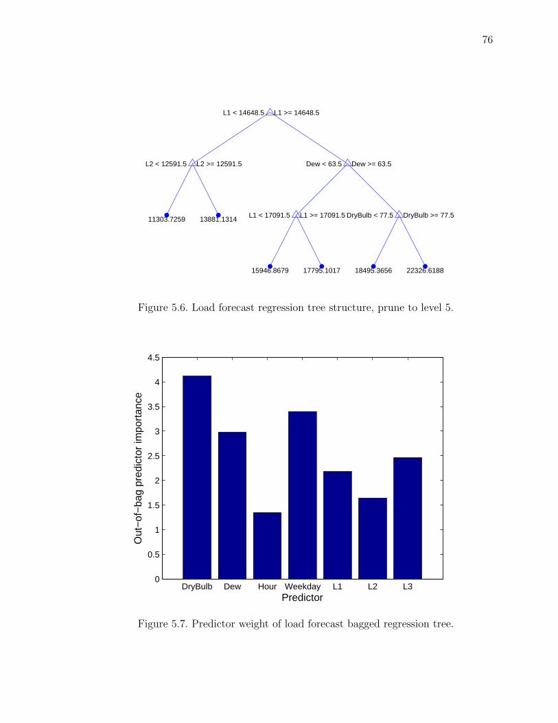
76
11303.7259 13881.1314
15946.8679 17795.1017 18495.3656 22326.6188
L1 < 14648.5
L2 < 12591.5 Dew < 63.5
L1 < 17091.5 DryBulb < 77.5
L1 >= 14648.5
L2 >= 12591.5 Dew >= 63.5
L1 >= 17091.5 DryBulb >= 77.5
Figure 5.6. Load forecast regression tree structure, prune to level 5.
DryBulb Dew Hour Weekday L1 L2 L30
0.5
1
1.5
2
2.5
3
3.5
4
4.5
Predictor
Out
−of
−ba
g pr
edic
tor
impo
rtan
ce
Figure 5.7. Predictor weight of load forecast bagged regression tree.
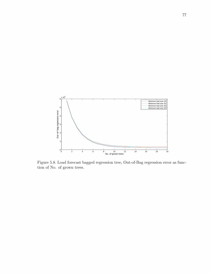
77
0 2 4 6 8 10 12 14 16 18 200
1
2
3
4
5
6x 10
6
No. of grown trees
Out
−of
−ba
g re
gres
sion
err
or
Minimum leaf size 10Minimum leaf size 20Minimum leaf size 40Minimum leaf size 50
Figure 5.8. Load forecast bagged regression tree, Out-of-Bag regression error as func-tion of No. of grown trees.
78
6. CONCLUSIONS
Conclusion We have developed a milliseconds resolution dynamical model for CSPs
with detailed components including solar reflectors (heliostats), power towers, salt
tanks, boiler, turbines, generators, piping as well as instant fatigue life model and
demand forecast model. This integrated model platform allows researchers to run
different control and optimization algorithms in real time and test their impact on
system transients—which are the major cause of system failure and life cycle reduc-
tion. We have also shown in the paper that with proper control and optimization
algorithm applied to the model, the panel life time can be increased and therefore
the system LCOE may be reduced as well, making CSP plants more financially com-
petitive with the traditional coal fired plants.
We have demonstrated a three-level controller architecture using multi-input-
multi-output (MIMO) control for CSP plants that can be implemented on existing
plants to improve performance, reliability, and extend the life of the plant. This archi-
tecture makes the optimization of the performance on multiple time scales including:
reactive level (regulation to temperature set points), tactical level (adaptation of
temperature set points), and strategic level (trading off fatigue life due to thermal
cycling and current production) possible. This controller contribute significantly to-
wards the Sunshot goal of 0.06/kWh(e), while responding to both market dynamics
and changes in solar irradiance such as due to passing clouds. The controller also
takes into consideration of plant disturbance and measurement noise in the controller
design.
Future work This integrated CSP model provides a platform that allows more
interesting problems to be quickly studied. Few of the interesting problems that can
be easily implemented on this platform would be:

79
1. LQR/LTR and H∞ controller design to enhance receiver controller stability
and robustness.
2. Linear Parameter Varying (LPV) and Linear Matrix Inequalities (LMI) con-
troller design for large scale disturbance and middle time scale optimization for
heliostat-receiver subsystem.
3. Integration of PV and CSP for electricity output optimization.
4. Economics and environment trade-off for heliostat field optimization.
5. Heat storage design optimization based on electricity supply-demand optimiza-
tion.
6. Modelling of CSP trough system and controllers design for this system.

LIST OF REFERENCES
80
LIST OF REFERENCES
[1] B. Canavan M. Mendelsohn, T. Lowder. Utility-scale concentrating solar powerand photovoltaic projects: A technology and market overview. Technical report,National Renewable Energy Laboratory (NREL), Golden, CO., 2012.
[2] K. Johnson and S. Page. Utility-scale solar projects in the united states operat-ing, under construction, or under development. Technical report, Solar EnergyIndustries Association (SEIA), 2011.
[3] T. Kimbis and S. Fenn. Solar market insight report 2012, q1. Technical report,Solar Energy Industries Association (SEIA), 2012.
[4] B. Hoffschmidt, S. Alexopoulos, C. Rau, J. Sattler, A. Anthrakidis, C. Boura,B. Connor, and P. Hilger. Concentrating solar power. In Comprehensive Renew-able Energy, pages 595 – 636. Elsevier, Oxford, 2012.
[5] J. V. Scoter and D. Rogers. Sierra suntower fact sheet. Technical report, eSolarCo., 2010.
[6] M. Mehos. Genesis solar energy project fact sheet. Technical report, NationalRenewable Energy Laboratory, 2009.
[7] T. Wendelin. Concentrating solar power projects: Solana. Technical report,National Renewable Energy Laboratory, 2010.
[8] P. K. Falcone. A handbook for solar central receiver design. Technical report,Sandia National Labs., Livermore, CA (USA), 1986.
[9] E. Sani, L. Mercatelli, P. Sansoni, L. Silvestroni, and D. Sciti. Spectrally selec-tive ultra-high temperature ceramic absorbers for high-temperature solar plants.Journal of Renewable and Sustainable Energy, 4(3), 2012.
[10] G. Augsburger and D. Favrat. Modelling of the receiver transient flux distributiondue to cloud passages on a solar tower thermal power plant. Solar Energy, 87:42– 52, 2013.
[11] D. O. Harris, C. H. Wells, H. J. Grunloh, R. H. Ryder, J. M. Bloom, C. C.Schultz, and R. Viswanathan. Bless-boiler life evaluation and simulation system:A computer code for reliability analysis of headers and piping. American Societyof Mechanical Engineers, Pressure Vessels and Piping Division, 251:17–17, 1993.
[12] G. Grossman and M. T. Heath. Simultaneous heat and mass transfer in absorp-tion of gases in turbulent liquid films. International Journal of Heat and MassTransfer, 27(12):2365 – 2376, 1984.
[13] G. J. Kolb, R. Davenport, D. Gorman, R. Lumia, R. Thomas, and M. Donnelly.Heliostat cost reduction. pages 1077–1084, 2007.
81
[14] S. A. Kalogirou. Solar energy collectors. In Solar Energy Engineering, pages 121– 217. Academic Press, Boston, 2009.
[15] I. Reda and A. Andreas. Solar position algorithm for solar radiation applications(revised). Technical report, National Renewable Energy Laboratory, 2008.
[16] M. Schmitz, P. Schwarzbzl, R. Buck, and R. P.-Paal. Assessment of the potentialimprovement due to multiple apertures in central receiver systems with secondaryconcentrators. Solar Energy, 80(1):111 – 120, 2006.
[17] X. Wei, Z. Lu, W. Yu, and Z. Wang. A new code for the design and analysis ofthe heliostat field layout for power tower system. Solar Energy, 84(4):685 – 690,2010.
[18] C. J. Noone, M. Torrilhon, and A. Mitsos. Heliostat field optimization: A newcomputationally efficient model and biomimetic layout. Solar Energy, 86(2):792– 803, 2012.
[19] R. Pitz-Paal, N. B. Botero, and A. Steinfeld. Heliostat field layout optimizationfor high-temperature solar thermochemical processing. Solar Energy, 85(2):334– 343, 2011.
[20] M. Berenguel, F.R. Rubio, A. Valverde, P.J. Lara, M.R. Arahal, E.F. Camacho,and M. Lapez. An artificial vision-based control system for automatic heliostatpositioning offset correction in a central receiver solar power plant. Solar Energy,76(5):563 – 575, 2004.
[21] M. Guo, Z. Wang, J. Zhang, F. Sun, and X. Zhang. Determination of the angularparameters in the general altitudeazimuth tracking angle formulas for a heliostatwith a mirror-pivot offset based on experimental tracking data. Solar Energy,86(3):941 – 950, 2012.
[22] J. J. Guo, J. Y. Wu, R. Z. Wang, and S. Li. Experimental research and operationoptimization of an air-source heat pump water heater. Applied Energy, 88:4128–4138, April 2011.
[23] A. M. Clausing. An analysis of convective losses from cavity solar central re-ceivers. Solar Energy, 27(4):295 – 300, 1981.
[24] N. Singh, S.C. Kaushik, and R.D. Misra. Exergetic analysis of a solar thermalpower system. Renewable Energy, 19(12):135 – 143, 2000.
[25] A. Kurtbas and A. Durmust. Efficiency and exergy analysis of a new solar airheater. Renewable Energy, 29(9):1489 – 1501, 2004.
[26] M. J. Montes, A. Rovira, J. M. Martnez-Val, and A. Ramos. Proposal of a fluidflow layout to improve the heat transfer in the active absorber surface of solarcentral cavity receivers. Applied Thermal Engineering, 35(0):220 – 232, 2012.
[27] X. Yang, X. Yang, J. Ding, Y. Shao, F. G.F. Qin, and R. Jiang. Criteria forperformance improvement of a molten salt thermocline storage system. AppliedThermal Engineering, 48(0):24 – 31, 2012.
82
[28] A. Gil, M. Medrano, I. Martorell, A. Lzaro, P. Dolado, B. Zalba, and L. F.Cabeza. State of the art on high temperature thermal energy storage for powergeneration. part 1 concepts, materials and modellization. Renewable and Sus-tainable Energy Reviews, 14(1):31 – 55, 2010.
[29] Z. Yang and S. V. Garimella. Thermal analysis of solar thermal energy storagein a molten-salt thermocline. Solar Energy, 84(6):974 – 985, 2010.
[30] S. Flueckiger, Z. Yang, and S. V. Garimella. An integrated thermal and mechan-ical investigation of molten-salt thermocline energy storage. Applied Energy,88(6):2098 – 2105, 2011.
[31] A. Mawire, M. McPherson, R. R. J. van den Heetkamp, and S.J.P. Mlatho. Sim-ulated performance of storage materials for pebble bed thermal energy storage(tes) systems. Applied Energy, 86(78):1246 – 1252, 2009.
[32] T. M. Sanderson and G. T. Cunningham. Performance and efficient design ofpacked bed thermal storage systems. part 1. Applied Energy, 50(2):119 – 132,1995.
[33] L. F. Cabeza. Thermal energy storage. In Comprehensive Renewable Energy,pages 211 – 253. Elsevier, Oxford, 2012.
[34] M. Hannchen, S. Brckner, and A. Steinfeld. High-temperature thermal storageusing a packed bed of rocks - heat transfer analysis and experimental validation.Applied Thermal Engineering, 31(10):1798 – 1806, 2011.
[35] D. A. Plautz and H. F. Johnstone. Heat and mass transfer in packed beds.American Institute of Chemical Engineers, 1(2):193–199, 1955.
[36] S. Holland. Hitec heat transfer salt. Technical report, Brenntag Company.
[37] E. E. Gonzo. Estimating correlations for the effective thermal conductivity ofgranular materials. Chemical Engineering Journal, 90(3):299 – 302, 2002.
[38] R. Ekbom. Application of hip/pm technique for gas and steam turbines. MetalPowder Report, 45(4):284 – 289, 1990.
[39] A. Chaibakhsh and A. Ghaffari. Steam turbine model. Simulation ModellingPractice and Theory, 16(9):1145 – 1162, 2008.
[40] J. M. Medina-Flores and M. Picon-Nunez. Modelling the power production ofsingle and turbines. Chemical Engineering Science, 65(9):2811 – 2820, 2010.
[41] K. J. Astrom and R.D. Bell. Drum-boiler dynamics. Automatica, 36(3):363 –378, 2000.
[42] W. M. Lin, C. C. Tsai, and C. H. Lin. Analysing the linear equivalent circuitsof electromechanical systems for steam turbine generator units. Generation,Transmission Distribution, IET, 5(7):685 –693, july 2011.
[43] E. F. Fuchs and M. A.S. Masoum. Modeling and analysis of synchronous ma-chines. In Power Quality in Power Systems and Electrical Machines, pages 155– 207. Academic Press, Burlington, 2008.
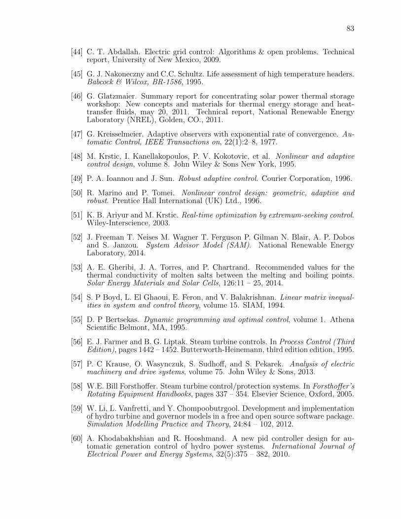
83
[44] C. T. Abdallah. Electric grid control: Algorithms & open problems. Technicalreport, University of New Mexico, 2009.
[45] G. J. Nakoneczny and C.C. Schultz. Life assessment of high temperature headers.Babcock & Wilcox, BR-1586, 1995.
[46] G. Glatzmaier. Summary report for concentrating solar power thermal storageworkshop: New concepts and materials for thermal energy storage and heat-transfer fluids, may 20, 2011. Technical report, National Renewable EnergyLaboratory (NREL), Golden, CO., 2011.
[47] G. Kreisselmeier. Adaptive observers with exponential rate of convergence. Au-tomatic Control, IEEE Transactions on, 22(1):2–8, 1977.
[48] M. Krstic, I. Kanellakopoulos, P. V. Kokotovic, et al. Nonlinear and adaptivecontrol design, volume 8. John Wiley & Sons New York, 1995.
[49] P. A. Ioannou and J. Sun. Robust adaptive control. Courier Corporation, 1996.
[50] R. Marino and P. Tomei. Nonlinear control design: geometric, adaptive androbust. Prentice Hall International (UK) Ltd., 1996.
[51] K. B. Ariyur and M. Krstic. Real-time optimization by extremum-seeking control.Wiley-Interscience, 2003.
[52] J. Freeman T. Neises M. Wagner T. Ferguson P. Gilman N. Blair, A. P. Dobosand S. Janzou. System Advisor Model (SAM). National Renewable EnergyLaboratory, 2014.
[53] A. E. Gheribi, J. A. Torres, and P. Chartrand. Recommended values for thethermal conductivity of molten salts between the melting and boiling points.Solar Energy Materials and Solar Cells, 126:11 – 25, 2014.
[54] S. P Boyd, L. El Ghaoui, E. Feron, and V. Balakrishnan. Linear matrix inequal-ities in system and control theory, volume 15. SIAM, 1994.
[55] D. P Bertsekas. Dynamic programming and optimal control, volume 1. AthenaScientific Belmont, MA, 1995.
[56] E. J. Farmer and B. G. Liptak. Steam turbine controls. In Process Control (ThirdEdition), pages 1442 – 1452. Butterworth-Heinemann, third edition edition, 1995.
[57] P. C Krause, O. Wasynczuk, S. Sudhoff, and S. Pekarek. Analysis of electricmachinery and drive systems, volume 75. John Wiley & Sons, 2013.
[58] W.E. Bill Forsthoffer. Steam turbine control/protection systems. In Forsthoffer’sRotating Equipment Handbooks, pages 337 – 354. Elsevier Science, Oxford, 2005.
[59] W. Li, L. Vanfretti, and Y. Chompoobutrgool. Development and implementationof hydro turbine and governor models in a free and open source software package.Simulation Modelling Practice and Theory, 24:84 – 102, 2012.
[60] A. Khodabakhshian and R. Hooshmand. A new pid controller design for au-tomatic generation control of hydro power systems. International Journal ofElectrical Power and Energy Systems, 32(5):375 – 382, 2010.
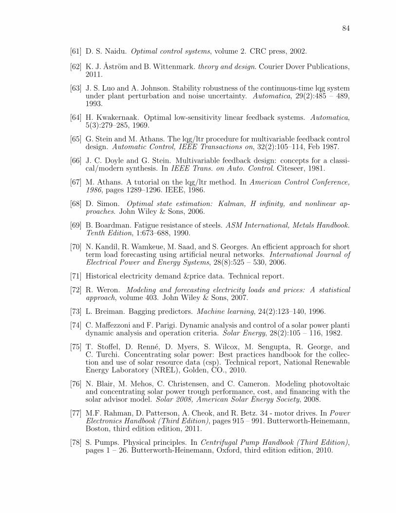
84
[61] D. S. Naidu. Optimal control systems, volume 2. CRC press, 2002.
[62] K. J. Astrom and B. Wittenmark. theory and design. Courier Dover Publications,2011.
[63] J. S. Luo and A. Johnson. Stability robustness of the continuous-time lqg systemunder plant perturbation and noise uncertainty. Automatica, 29(2):485 – 489,1993.
[64] H. Kwakernaak. Optimal low-sensitivity linear feedback systems. Automatica,5(3):279–285, 1969.
[65] G. Stein and M. Athans. The lqg/ltr procedure for multivariable feedback controldesign. Automatic Control, IEEE Transactions on, 32(2):105–114, Feb 1987.
[66] J. C. Doyle and G. Stein. Multivariable feedback design: concepts for a classi-cal/modern synthesis. In IEEE Trans. on Auto. Control. Citeseer, 1981.
[67] M. Athans. A tutorial on the lqg/ltr method. In American Control Conference,1986, pages 1289–1296. IEEE, 1986.
[68] D. Simon. Optimal state estimation: Kalman, H infinity, and nonlinear ap-proaches. John Wiley & Sons, 2006.
[69] B. Boardman. Fatigue resistance of steels. ASM International, Metals Handbook.Tenth Edition, 1:673–688, 1990.
[70] N. Kandil, R. Wamkeue, M. Saad, and S. Georges. An efficient approach for shortterm load forecasting using artificial neural networks. International Journal ofElectrical Power and Energy Systems, 28(8):525 – 530, 2006.
[71] Historical electricity demand &price data. Technical report.
[72] R. Weron. Modeling and forecasting electricity loads and prices: A statisticalapproach, volume 403. John Wiley & Sons, 2007.
[73] L. Breiman. Bagging predictors. Machine learning, 24(2):123–140, 1996.
[74] C. Maffezzoni and F. Parigi. Dynamic analysis and control of a solar power plantidynamic analysis and operation criteria. Solar Energy, 28(2):105 – 116, 1982.
[75] T. Stoffel, D. Renne, D. Myers, S. Wilcox, M. Sengupta, R. George, andC. Turchi. Concentrating solar power: Best practices handbook for the collec-tion and use of solar resource data (csp). Technical report, National RenewableEnergy Laboratory (NREL), Golden, CO., 2010.
[76] N. Blair, M. Mehos, C. Christensen, and C. Cameron. Modeling photovoltaicand concentrating solar power trough performance, cost, and financing with thesolar advisor model. Solar 2008, American Solar Energy Society, 2008.
[77] M.F. Rahman, D. Patterson, A. Cheok, and R. Betz. 34 - motor drives. In PowerElectronics Handbook (Third Edition), pages 915 – 991. Butterworth-Heinemann,Boston, third edition edition, 2011.
[78] S. Pumps. Physical principles. In Centrifugal Pump Handbook (Third Edition),pages 1 – 26. Butterworth-Heinemann, Oxford, third edition edition, 2010.

APPENDIX

85
A. APPENDIX
A.1 Solar Radiation, Temperature, Electricity Load Sensing and Mea-
surement
The Solar radiation and electricity loading profile serves as disturbance to the
control architect, therefore in order to enhance the control quality of CSP plant,
we need to first have a good measurement of current solar radiation and accurate
electricity loading information.
A.1.1 Solar Radiation Measurement
As discussed in chapter 2, a cloud can reduce the solar radiation from sun signifi-
cantly, as shown in figure A.1 from National Renewable Energy Laboratory, therefore
the cloud passing by the concentrating solar plant can introduce irradiation transients,
sustaining a strong thermal stress on receivers. This thermal stress can cause a de-
crease in receiver cyclic life and a decrease in solar absorption efficiency,as discussed
in [74].
Therefore, it is essential to estimate and do a real-time measurement of solar
irradiation, and develop control algorithm to avoid strong thermal stress.
Commonly used solar radiation measurement instrument includes:
Pyrheliometer : For direct normal solar radiation measurement.
Pyranometer : For global horizontal radiation measurement.
Thermopile detectors :Slow, expensive, flat spectral response.
Thermopile detectors :Fast, Low-Cost, with Reduced Spectral Response (fig-
ure A.2).
Shaded Pyranometer : For diffuse radiation measurement.
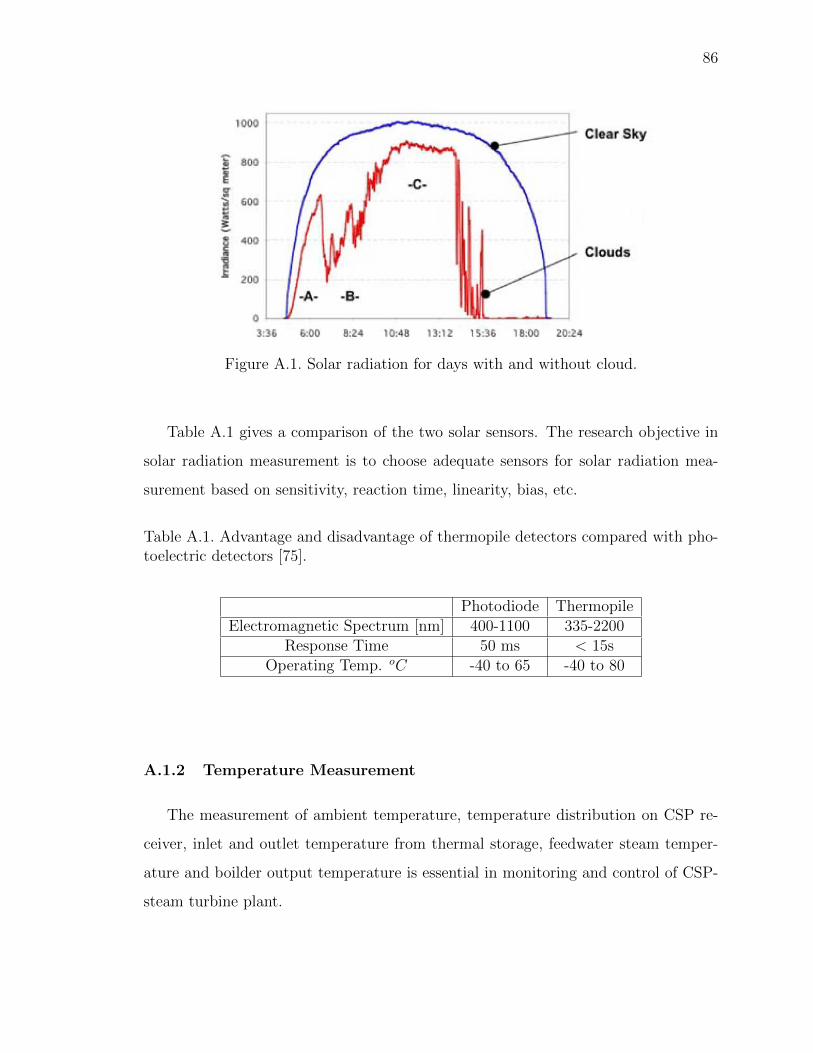
86
Figure A.1. Solar radiation for days with and without cloud.
Table A.1 gives a comparison of the two solar sensors. The research objective in
solar radiation measurement is to choose adequate sensors for solar radiation mea-
surement based on sensitivity, reaction time, linearity, bias, etc.
Table A.1. Advantage and disadvantage of thermopile detectors compared with pho-toelectric detectors [75].
Photodiode ThermopileElectromagnetic Spectrum [nm] 400-1100 335-2200
Response Time 50 ms < 15sOperating Temp. oC -40 to 65 -40 to 80
A.1.2 Temperature Measurement
The measurement of ambient temperature, temperature distribution on CSP re-
ceiver, inlet and outlet temperature from thermal storage, feedwater steam temper-
ature and boilder output temperature is essential in monitoring and control of CSP-
steam turbine plant.
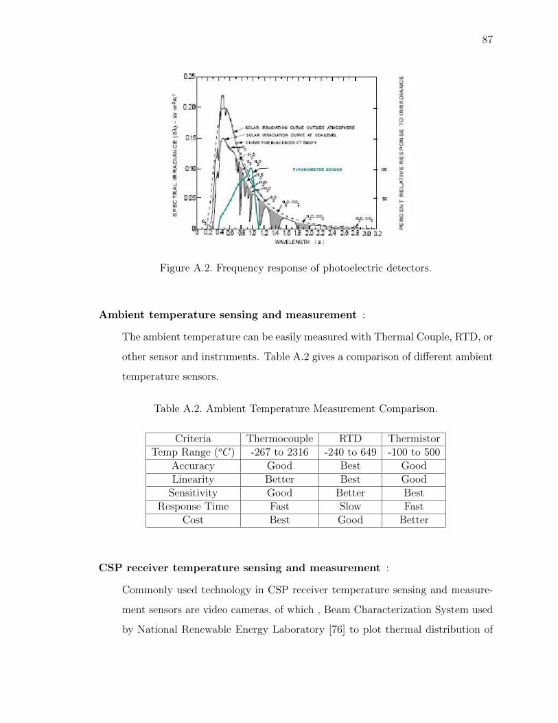
87
Figure A.2. Frequency response of photoelectric detectors.
Ambient temperature sensing and measurement :
The ambient temperature can be easily measured with Thermal Couple, RTD, or
other sensor and instruments. Table A.2 gives a comparison of different ambient
temperature sensors.
Table A.2. Ambient Temperature Measurement Comparison.
Criteria Thermocouple RTD ThermistorTemp Range (oC) -267 to 2316 -240 to 649 -100 to 500
Accuracy Good Best GoodLinearity Better Best Good
Sensitivity Good Better BestResponse Time Fast Slow Fast
Cost Best Good Better
CSP receiver temperature sensing and measurement :
Commonly used technology in CSP receiver temperature sensing and measure-
ment sensors are video cameras, of which , Beam Characterization System used
by National Renewable Energy Laboratory [76] to plot thermal distribution of
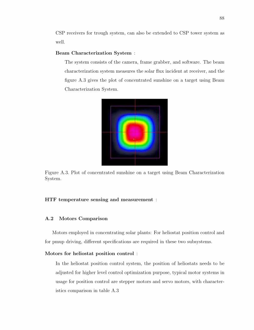
88
CSP receivers for trough system, can also be extended to CSP tower system as
well.
Beam Characterization System :
The system consists of the camera, frame grabber, and software. The beam
characterization system measures the solar flux incident at receiver, and the
figure A.3 gives the plot of concentrated sunshine on a target using Beam
Characterization System.
Figure A.3. Plot of concentrated sunshine on a target using Beam CharacterizationSystem.
HTF temperature sensing and measurement :
A.2 Motors Comparison
Motors employed in concentrating solar plants: For heliostat position control and
for pmup driving, different specifications are required in these two subsystems.
Motors for heliostat position control :
In the heliostat position control system, the position of heliostats needs to be
adjusted for higher level control optimization purpose, typical motor systems in
usage for position control are stepper motors and servo motors, with character-
istics comparison in table A.3
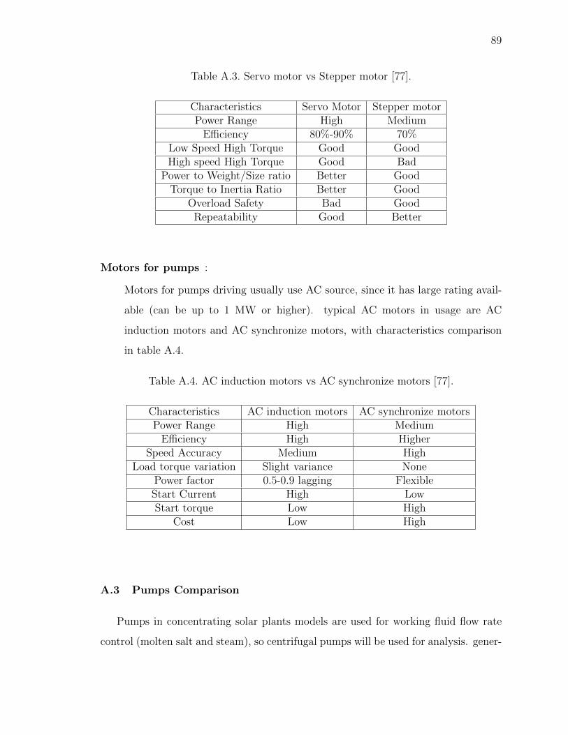
89
Table A.3. Servo motor vs Stepper motor [77].
Characteristics Servo Motor Stepper motorPower Range High Medium
Efficiency 80%-90% 70%Low Speed High Torque Good GoodHigh speed High Torque Good Bad
Power to Weight/Size ratio Better GoodTorque to Inertia Ratio Better Good
Overload Safety Bad GoodRepeatability Good Better
Motors for pumps :
Motors for pumps driving usually use AC source, since it has large rating avail-
able (can be up to 1 MW or higher). typical AC motors in usage are AC
induction motors and AC synchronize motors, with characteristics comparison
in table A.4.
Table A.4. AC induction motors vs AC synchronize motors [77].
Characteristics AC induction motors AC synchronize motorsPower Range High Medium
Efficiency High HigherSpeed Accuracy Medium High
Load torque variation Slight variance NonePower factor 0.5-0.9 lagging FlexibleStart Current High LowStart torque Low High
Cost Low High
A.3 Pumps Comparison
Pumps in concentrating solar plants models are used for working fluid flow rate
control (molten salt and steam), so centrifugal pumps will be used for analysis. gener-
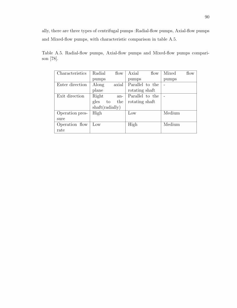
90
ally, there are three types of centrifugal pumps :Radial-flow pumps, Axial-flow pumps
and Mixed-flow pumps, with characteristic comparison in table A.5.
Table A.5. Radial-flow pumps, Axial-flow pumps and Mixed-flow pumps compari-son [78].
Characteristics Radial flowpumps
Axial flowpumps
Mixed flowpumps
Enter direction Along axialplane
Parallel to therotating shaft
-
Exit direction Right an-gles to theshaft(radially)
Parallel to therotating shaft
-
Operation pres-sure
High Low Medium
Operation flowrate
Low High Medium

VITA

91
VITA
Luo,Qi received the Bachelor’s degree from Shanghai Jiao Tong University (SJTU),
Shanghai, China, in 2009. During 2008-2009, he was undergraduate exchange student
in Purdue University. He is now a graduate student in Department of Mechanical
Engineering, Purdue University, Indiana, USA. His current research interests include
analysis and control of power system.