Embed Size (px)
Citation preview

Control of wireless networks with flow level dynamics underconstant time scheduling
Long Bao Le Æ Ravi R. Mazumdar
� Springer Science+Business Media, LLC 2009
Abstract We consider a network control problem for
wireless networks with flow level dynamics under the
general k-hop interference model. In particular, we inves-
tigate the control problem in low load and high load
regimes. In the low load regime, we show that the network
can be stabilized by a regulated maximal scheduling policy
considering flow level dynamics if the offered load satisfies
a constraining bound condition. Because maximal sched-
uling is a general scheduling rule whose implementation is
not specified, we propose a constant-time and distributed
scheduling algorithm for a general k-hop interference
model which can approximate the maximal scheduling
policy within an arbitrarily small error. Under the stability
condition, we show how to calculate transmission rates for
different user classes such that the long-term (time aver-
age) network utility is maximized. This long-term network
utility captures the real network performance due to the
fact that under flow level dynamics, the number of users
randomly change so instantaneous network utility maxi-
mization does not result in useful network performance.
Our results imply that congestion control is unnecessary
when the offered load is low and optimal user rates can be
determined to maximize users’ long-term satisfaction. In
the high load regime where the network can be unstable
under the regulated maximal scheduling policy, we propose
a cross-layer congestion control and scheduling algorithm
which can stabilize the network under arbitrary network
load. Through extensive numerical analysis for some typ-
ical networks, we show that the proposed scheduling
algorithm has much lower overhead than other existing
queue-length-based constant-time scheduling schemes in
the literature, and it achieves performance much better than
the guaranteed bound.
Keywords Flow level dynamics � Capacity region �Constant-time scheduling � Network stability �Maximal matching � k-Hop interference model
1 Introduction
Resource allocation in communication networks has been
an active research topic for the last several years. While
optimal rate control in wired networks can be achieved by a
distributed algorithm [1–4], solving this problem in wire-
less networks is much more challenging. In fact, the bot-
tleneck of the resource allocation problem in wireless
networks lies in the scheduling sub-problem [5, 6]. The
difficulty of the scheduling sub-problem comes from the
interference coupling of simultaneous transmissions from
different wireless links in the network.
In general, interference coupling in wireless networks
depends on the communication technologies employed at
the physical layer. For example, the node exclusive inter-
ference model can be assumed for Bluetooth networks or
FH-CDMA networks [7, 8]. This interference model is also
referred to as one-hop interference model. For the 802.11
WLAN with four-way handshake (i.e., with RTS/CTS), the
two-hop interference model is implicitly assumed in the
MAC protocol. Moreover, it has been shown in [9] that in
This paper was presented in part at CISS’2008, Princeton, NJ, USA.
L. B. Le
Massachusetts Institute of Technology, Cambridge, MA, USA
e-mail: [email protected]
R. R. Mazumdar (&)
Department of Electrical and Computer Engineering,
University of Waterloo, Waterloo, ON, Canada
e-mail: [email protected]
123
Wireless Netw
DOI 10.1007/s11276-009-0208-8

certain network settings and QoS requirements, neither
one-hop nor two-hop interference model is optimal to
achieve the maximum number of simultaneous transmis-
sions in the network.
In [9] the authors proposed a general interference model
called a k-hop interference model which is determined by a
single parameter k. For this interference model, wireless
links k ? 1 or more hops away from one another can be
scheduled to transmit data at the same time. Developing a
joint resource allocation and scheduling algorithm for this
k-hop interference model is, therefore, much more desir-
able than working with a special case of this general
interference model. This is indeed what we will pursue in
this paper.
Regarding the scheduling problem in wireless networks,
there are several optimal and suboptimal schemes proposed
in the literature. In a seminal paper [10], Tassiulas and
Ephremides proposed an optimal back-pressure policy
which achieves the maximum capacity region. This
scheduling policy is, however, centralized and computa-
tionally expensive. In [11], a randomized linear-complexity
scheduling algorithm was proposed where a transmission
schedule in time slot t was constructed by choosing the
schedule with larger total weight between the schedule in
time slot t-1 and a newly-generated one in time slot t. This
idea was used to develop distributed throughput-optimal
scheduling policies in [12–14] for one-hop and two-hop
interference models. Note that these scheduling algorithms
achieve full utilization of wireless networks with respect to
what remains in the data transmission phase only. Specif-
ically, a large amount of bandwidth has been wasted to
exchange control information in the schedule construction
phase which would otherwise be used for data transmis-
sion. In general, the amount of scheduling overhead grows
with the network size for these throughput-optimal sched-
uling policies.
Due to implementation constraints, the time slot interval
is usually limited to a few milliseconds as in most current
wireless systems. Therefore, developing a scheduling
algorithm with low and constant-time overhead is very
desirable. In fact, some queue-length-based constant-time
scheduling algorithms were proposed for one and two hop
interference models [15–17] recently in the literature.
These scheduling algorithms only achieve a guaranteed
faction of the capacity region but they have constant time
overhead. For practical implementation, collecting queue
length information may be difficult, and it will create fur-
ther overhead. A more general maximal scheduling policy
was considered in [18, 19] where several throughput per-
formance bounds were investigated. However, implemen-
tation of this general scheduling policy and investigation of
its actual performance in typical wireless networks were
not conducted in these papers.
In practice, it is desired that each wireless node only
communicates with its neighbors (e.g., those whose trans-
missions interfere with that of the underlying node) to
construct a transmission schedule in each time slot. Also,
scheduling algorithms should work for a general class of
interference models (e.g., k-hop interference model [9]).
Another aspect which was ignored by most existing works
in the literature is that no conflict-free schedule is available
to exchange control information at the beginning of each
time slot. Therefore, control information can only be
exchanged by using contention-based transmissions which
renders information exchange more than one hop away a
time-consuming operation. Also, it is important to quantify
amount of time/overhead used to construct the schedule
and to develop explicit procedure to exchange control
information in each time slot.
In this paper, we show the performance guarantee of the
regulated maximal scheduling policy in wireless networks
considering flow level dynamics. Regulated maximal
scheduling is a combination of the maximal scheduling
policy [18, 19] and traffic regulator implementation at each
wireless link. In fact, it has been shown in both manufac-
turing systems and telecommunication networks that when
routing paths form loops the system/network can be driven
into unstable operation even if the traffic rate at each
machine/router is strictly smaller than its service rate [20,
21]. In [22], it has been shown that employment of traffic
regulators can stabilize the network even if routing paths
form loops in the network. This is the reason why we
employ traffic regulators at all wireless links in this paper
even though it may not be neccessary to do so if routing
paths do not form loops in the network.
Regulated maximal scheduling is a general rule, and we
propose a constant-time and distributed algorithm to
implement it in each time slot. We show that the proposed
scheduling algorithm can approximate the regulated max-
imal scheduling policy within an arbitrarily small error.
The proposed scheduling algorithm works for the general
k-hop interference model and does not require queue length
information. Moreover, we explicitly describe how wire-
less links coordinate their contentions to construct the
schedule in each time slot. Given the fact that the sched-
uling algorithm is randomized and the number of users
dynamically changes, instantaneous network utility maxi-
mization would not result in good network performance.
Because of this, we are interested in finding transmission
rate for each user class which achieves maximum long-
term (time average) utility. In fact, we show that there
exists optimal transmission rates for all user classes to
achieve such maximum long-term utility. When the net-
work load is high, we propose a cross-layer congestion
control algorithm which can stabilize the network for
arbitrary network load.
Wireless Netw
123

The results presented in this paper have several impor-
tant implications for system implementation. First, we do
not need to perform congestion control in low network load
even with flow level dynamics. In fact, performing con-
gestion control requires frequent feedback of congestion
prices along routing paths to source nodes to update their
transmission rates [1–4]. This feedback of congestion pri-
ces consumes a significant amount bandwidth which would
be used to improve transmission rate of useful traffic
otherwise. Also, implementation issues such as asynchro-
nous [8] and noisy [23] feedback due to congestion control
operations can be completely avoided. Moreover, this is an
interesting finding given the fact that recent works propose
to employ congestion control algorithms to stabilize the
network [5, 24] under low network load when flow level
dynamics is considered. Second, the problem of network
utility maximization can be decoupled from that of stabi-
lizing the network. Specifically, the network can be stabi-
lized by implementing traffic regulators at wireless links
together with a suitable scheduling mechanism. In fact, we
show via numerical examples that using congestion control
algorithm to stabilize the network in low load actually
degrades the long-term network utility considerably. Pre-
liminary results of this paper was presented in [25].
The remainder of this paper is organized as follows. We
describe the system models and performance bounds in
Sect. 2. Performance guarantee of the regulated maximal
scheduling policy is presented in Sect. 3. In Sect. 4, we
present the distributed scheduling algorithm to approximate
the maximal scheduling policy. We derive the optimal
transmission rates to achieve long-term utility maximization
in Sect. 5. The cross-layer congestion control and scheduling
algorithm in the high load regime is described in Sect. 6.
Some numerical results are presented in Sect. 7, and Sect. 8
states the conclusion. For notational convenience, we will
put elements of different measures into the corresponding
vectors. For example, the vector of transmission rates will be
denoted by x~where xs is its s-th element which is the trans-
mission rate of class-s users. In the following, we will use two
terms matching and scheduling interchangeably.
2 System models and performance bound
We model a wireless network as a directed graph G = (V,
E) where V is the set of wireless nodes and E is the set of
wireless links. A wireless link from node i to node j exists
if node j can correctly receive information transmitted by
node i. In practice, existence of such a link depends on
transmission power, path loss, fading, interference, desired
bit error rate and other factors.
We assume that there are S classes of users each of
which is associated with a fixed routing path from a source
node to a destination node. The user routes are stored in an
incidence matrix ½Hks � where Hk
s ¼ 1 if link k is on the route
of class-s users and Hks ¼ 0 otherwise. Users of class s
arrive to the network with rate ks and each brings a file for
transfer whose size is exponentially distributed with mean
1/ls. The offered load by class-s users is, therefore, qs ¼ks=ls: The vector of offered load will be denoted as q~¼½q1; q2; . . .; qS�: We assume that users of each class transmit
at the same rate.
Interference constraints are denoted by a contention
matrix ½Cij�i;j2E: Specifically, link i is said to interfere with
link j if Cij = 1 and Cij = 0 otherwise. This general
notation of the interference relationship is used to describe
the capacity region and to derive the performance guar-
antee of the regulated maximal matching policy in this
section and Sect. 3 only. The k-hop interference model is a
special class of this general interference relationship. The
k-hop interference model is assumed in all other sections.
In this paper, we do not consider effects of channel
fading/capture in modeling interference/collision among
concurrent transmissions on different wireless links [26–28]
even though they can impact the interference in a neigh-
borhood. Channel fading/capture effects have been inves-
tigated for a single-hop wireless networks where multiple
users communicate with a single base station or an access
point in [26, 27]. Consideration of fading/capture effects for
multihop case is much more involved which is beyond the
scope of this paper. We assume a time-slotted system where
time slots are of unit duration. Link l can transmit at rate Rl
if its interfering links are not scheduled to transmit in a same
time slot. In the following, we provide some important
definitions which will be used throughout the paper.
Definition 1 Interference set Il of link l is the set of links
which interfere with link l, i.e.,
Il ¼ k 2 E : Ckl ¼ 1f g: ð1Þ
Definition 2 Interference degree dI(l) of link l is the
maximum number of links in its interference set which do
not interfere with each other.
Definition 3 Interference degree dI(G) of graph G is the
maximum interference degree of its links, i.e., dIðGÞ ¼maxl2E dIðlÞ:
Capacity region is defined to be the set of traffic load
such that the network can be stabilized by some scheduling
policy. Here, network stability means all individual queues
in the network have bounded average queue backlogs. Note
that the bounded average queue backlogs imply that the
average number of users of all user classes is bounded by
invoking the Little’s law. In [10], capacity region for
wireless networks is well characterized. In particular,
capacity region is given by the set
Wireless Netw
123

X ¼ q~ :XS
s¼1
Hlsqs
Rl
" #
l2E
2 CoðRÞ( )
ð2Þ
where CoðRÞ is the convex hull of all link schedulesR that
satisfy the constraints imposed by the underlying interfer-
ence model. A scheduling policy is said to be throughput
optimal if it stabilizes the network for all offered load
within the capacity region X.
We assume that a new schedule is constructed in the first
phase which is used to transmit data in the second phase of
each time slot. Traffic flows in the network may traverse
one hop or multiple hops. For the multiple-hop case, we
assume that traffic of each user class is regulated before
entering a transmission queue for being transfered over each
wireless link. The employment of regulators was previously
proposed by Humes to stabilize manufacturing systems [22]
which have been shown to be unstable in some cases due to
cycles of material flow [20]. Regulators were recently used
in wireless networks [8, 18]. A k-regulator associated with
link l generates packets to transmission queue of link l with
a maximum rate of k. A regulator can be implemented as
follows. In each time slot, a k-regulator associated with link
l checks the corresponding regulator queue. If the queue
length is greater than link capacity Rl then it transfers Rl
units of data to the transmission queue with probability k/Rl.
Otherwise, it transfers nothing. The regulator implementa-
tion is illustrated in Fig. 1.
In this paper, we assume a maximal scheduling policy
which was investigated in [18, 19]. The maximal sched-
uling rule can be described as follows. For any link l [ E
with transmission queue length larger than or equal to the
link capacity in any time slot, it is required that at least one
link in its interference set Il be scheduled. Specifically, if
Ql/Rl C 1 (where Ql is the queue length of transmission
queue for link l), we requireX
k2Il
pk � 1 ð3Þ
where pk = 1 if link k is scheduled and pk = 0 otherwise.
Due to the combination of maximal scheduling and regulator
implementation, the resulting scheduling will be called
regulated maximal scheduling in the following. Note that
maximal scheduling is a general scheduling rule without
specific implementation. We will present a constant time and
distributed scheduling algorithm which approximates the
maximal scheduling in Sect. 4. The following performance
bound of the maximal scheduling policy was proved in [19,
24], it is restated here for completeness.
Lemma 1 For all traffic load q~ within the capacity
region defined in (2), we have
X
k2Il
XS
s¼1
Hks qs
Rk� dIðlÞ; 8l 2 E: ð4Þ
This upper bound will be used to quantify the throughput
guarantee of the regulated maximal scheduling policy in the
next section.
3 Performance of the regulated maximal matching
scheme
In this section, we show that the network is stable under the
regulated maximal scheduling when the offered load sat-
isfies a specific condition. We assume that a ðqs þ k�Þ-regulator is employed at k-th hop on the route of class-s
users. It is worth mentioning that the following stability
result is similar in spirit to that in [18], although there is
an important difference here. In fact, we capture flow
dynamics in this paper while the authors in [18] only
considered dynamics at the packet level. In [5] and [24],
the authors captured flow dynamics but their stability
results were established assuming that a cross-layer con-
gestion control algorithm is emplyed. In this paper, we
show that network stability can be achieved without using
any congestion control mechanism if the traffic load is
sufficiently low. Hence, bandwidth wasted for collecting
and transmissions of congestion prices to update trans-
mission rates can be used to improve network throughput
performance. The stability result is stated in the following
proposition.
Proposition 1 If the traffic load satisfies
X
k2Il
XS
s¼1
Hks qs
Rk\1; 8l 2 E ð5Þ
then the network is stable under the regulated maximal
scheduling policy. This condition will be called a con-
straining bound in the following.
Proof The proof is in Appendix 1. h
Note that this constraining bound is tight in the sense that
the network can become unstable with any arbitrarily small
increase of the bound (i.e., the right hand side of (5) becomes
1 ? j for any j[ 0). This fact was proved in several papers
(for example, see [18, 19]). In the following, we state the
performance guarantee for the regulated maximal schedul-
ing policy.
Lemma 2 The regulated maximal scheduling policy
achieves 1/dI(G) capacity region.Fig. 1 Regulator implementation at each wireless link
Wireless Netw
123

Proof The proof follows directly by comparing the upper
and constraining bounds on capacity region in (4) and (5),
respectively, and using the definition of dI(G). h
4 Distributed scheduling algorithm
As mentioned before, maximal scheduling is a general rule
whose implementation is not specified. In this section, we
present a distributed scheduling algorithm which approxi-
mates the maximal scheduling policy in each time slot
within an arbitrarily small error. In fact, the proposed
algorithm will include the BP-SIM scheduling algorithm
[17] proposed for the node exclusive (i.e., one-hop) inter-
ference model as a special case. Our proposed algorithm
works with the general k-hop interference model. Also, in
contrast to the existing queue-length-based scheduling
algorithms [16, 17], in our algorithm each node with
incident backlogged links does not require queue length
information of other links in its neighborhood to construct
the transmission schedule. In addition, the proposed algo-
rithm is fully distributed, and it has constant time overhead
which does not grow with the network size. Our proposed
algorithm is, therefore, much more flexible and general
than existing ones in the literature. For ease of reference,
we will refer to our scheduling algorithm as random
approximate maximal matching (RAMM) scheduling in
the following.
4.1 Algorithm description
The RAMM algorithm is run in the first phase of each time
slot. Specifically, we divide each time slot into two phases:
a scheduling phase and a data transmission phase. The
transmission schedule is constructed in the scheduling
phase, and it is used to transmit data in the data trans-
mission phase. The scheduling phase is further divided into
K rounds each of which contains B mini-slots. In each
round, new links are added to the current transmission
schedule. The transmission schedule obtained at the end of
the K-th round will be used to transmit data in the data
transmission phase. In addition, only wireless links whose
queue lengths are larger than the link capacity are sched-
uled by the algorithm in each time slot. The time slot
structure of the RAMM algorithm is illustrated in Fig. 2.
Links are added to the schedule in each round through a
matching request and matching acknowledgment message
exchange as follows. At the beginning of each round, each
active node (the notion of active/inactive nodes will be
clarified shortly) decides to be left or right with probability
1/2. Nodes becoming right wait to receive matching
requests from their neighboring nodes. Backlogged links
are added to the schedule in each round as follows. Each
left node with at least one backlogged outgoing link (i.e., a
link from this node to one of its neighbors) will choose a
random backoff in [1, B]. When the backoff expires, a left
node will choose one of its backlogged neighbors randomly
to send a matching request if it has not heard any matching
requests transmitted by other nodes so far in the round. A
right node which receives a matching request will reply
with a matching acknowledgment message, and the cor-
responding link is added to the schedule. We assume that if
two or more matching requests are transmitted in one mini-
slot, collision occurs and no matching acknowledgment
message is transmitted.
In each round, we require that if a link is added to the
transmission schedule, all wireless links in its interference
set not be added to the transmission schedule in subsequent
rounds. This requirement guarantees that we will obtain a
conflict-free transmission schedule at the end of the
scheduling phase. It is observed that this requirement can
be easily achieved by the one-hop interference model.
Specifically, for the one-hop interference model after a link
is added to the schedule, both its transmitting and receiving
nodes will not transmit and reply to any matching requests
in subsequent rounds.
For a general k-hop interference model with k C 2, by
using physical carrier sensing during the scheduling phase
(as in a CSMA/CA protocol [29]) when a link is added to
the schedule, all nodes within k-1 hops from both the
transmitting and receiving nodes of the link are aware of
this (by sensing the matching request and matching
acknowledgment messages). Hence, they will not transmit
or reply to any matching requests in subsequent rounds.
Note that nodes within k-1 hops from either the trans-
mitting or receiving node of an added link are inside an
interference range of the newly-added link. Therefore, by
choosing an appropriate carrier sense threshold [29], this
requirement can be easily satisfied.
Nodes within k-1 hops from the transmitting and
receiving nodes of any links in the schedule are called
inactive nodes. All other nodes are active ones. Note that
any inactive node will remain inactive until the end of the
scheduling phase. In general, the number of nodes partic-
ipating in the schedule construction process reduces rapidly
over consecutive rounds. Because new links are added to
the existing schedule in each round, the transmission
schedule at the end of the scheduling phase wouldFig. 2 Timing diagram of the RAMM scheduling algorithm
Wireless Netw
123
approximate well the maximal schedule if B and K are
large enough. We will show the performance guarantee of
the proposed scheduling algorithm in the next subsection.
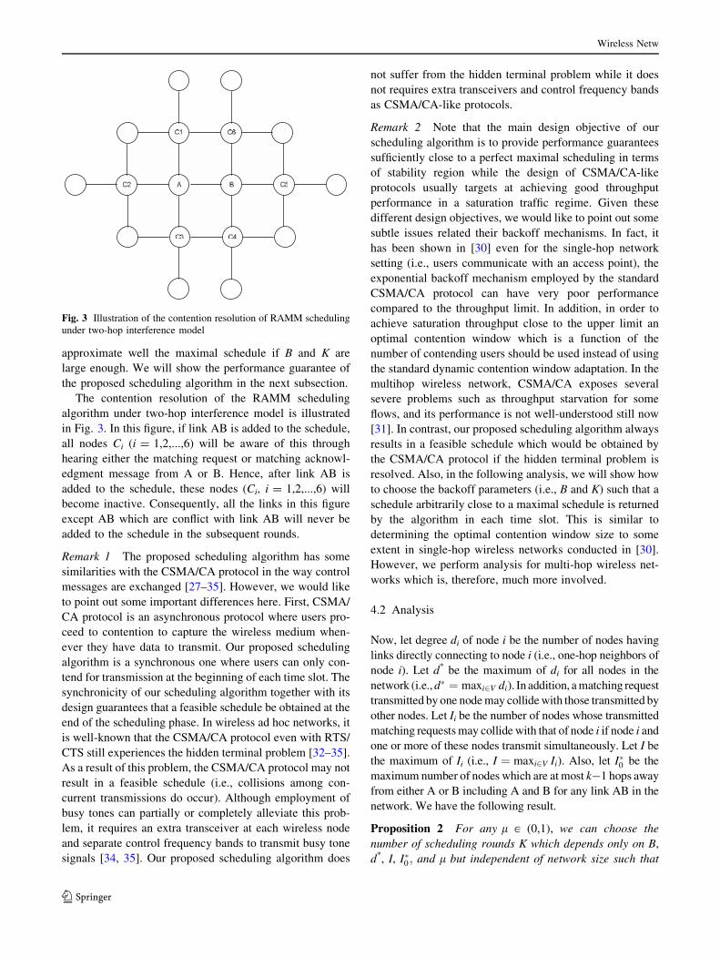
The contention resolution of the RAMM scheduling
algorithm under two-hop interference model is illustrated
in Fig. 3. In this figure, if link AB is added to the schedule,
all nodes Ci (i = 1,2,...,6) will be aware of this through
hearing either the matching request or matching acknowl-
edgment message from A or B. Hence, after link AB is
added to the schedule, these nodes (Ci, i = 1,2,...,6) will
become inactive. Consequently, all the links in this figure
except AB which are conflict with link AB will never be
added to the schedule in the subsequent rounds.
Remark 1 The proposed scheduling algorithm has some
similarities with the CSMA/CA protocol in the way control
messages are exchanged [27–35]. However, we would like
to point out some important differences here. First, CSMA/
CA protocol is an asynchronous protocol where users pro-
ceed to contention to capture the wireless medium when-
ever they have data to transmit. Our proposed scheduling
algorithm is a synchronous one where users can only con-
tend for transmission at the beginning of each time slot. The
synchronicity of our scheduling algorithm together with its
design guarantees that a feasible schedule be obtained at the
end of the scheduling phase. In wireless ad hoc networks, it
is well-known that the CSMA/CA protocol even with RTS/
CTS still experiences the hidden terminal problem [32–35].
As a result of this problem, the CSMA/CA protocol may not
result in a feasible schedule (i.e., collisions among con-
current transmissions do occur). Although employment of
busy tones can partially or completely alleviate this prob-
lem, it requires an extra transceiver at each wireless node
and separate control frequency bands to transmit busy tone
signals [34, 35]. Our proposed scheduling algorithm does
not suffer from the hidden terminal problem while it does
not requires extra transceivers and control frequency bands
as CSMA/CA-like protocols.
Remark 2 Note that the main design objective of our
scheduling algorithm is to provide performance guarantees
sufficiently close to a perfect maximal scheduling in terms
of stability region while the design of CSMA/CA-like
protocols usually targets at achieving good throughput
performance in a saturation traffic regime. Given these
different design objectives, we would like to point out some
subtle issues related their backoff mechanisms. In fact, it
has been shown in [30] even for the single-hop network
setting (i.e., users communicate with an access point), the
exponential backoff mechanism employed by the standard
CSMA/CA protocol can have very poor performance
compared to the throughput limit. In addition, in order to
achieve saturation throughput close to the upper limit an
optimal contention window which is a function of the
number of contending users should be used instead of using
the standard dynamic contention window adaptation. In the
multihop wireless network, CSMA/CA exposes several
severe problems such as throughput starvation for some
flows, and its performance is not well-understood still now
[31]. In contrast, our proposed scheduling algorithm always
results in a feasible schedule which would be obtained by
the CSMA/CA protocol if the hidden terminal problem is
resolved. Also, in the following analysis, we will show how
to choose the backoff parameters (i.e., B and K) such that a
schedule arbitrarily close to a maximal schedule is returned
by the algorithm in each time slot. This is similar to
determining the optimal contention window size to some
extent in single-hop wireless networks conducted in [30].
However, we perform analysis for multi-hop wireless net-
works which is, therefore, much more involved.
4.2 Analysis
Now, let degree di of node i be the number of nodes having
links directly connecting to node i (i.e., one-hop neighbors of
node i). Let d* be the maximum of di for all nodes in the
network (i.e., d� ¼ maxi2V di). In addition, a matching request
transmitted by one node may collide with those transmitted by
other nodes. Let Ii be the number of nodes whose transmitted
matching requests may collide with that of node i if node i and
one or more of these nodes transmit simultaneously. Let I be
the maximum of Ii (i.e., I ¼ maxi2V Ii). Also, let I�0 be the
maximum number of nodes which are at most k-1 hops away
from either A or B including A and B for any link AB in the
network. We have the following result.
Proposition 2 For any l [ (0,1), we can choose the
number of scheduling rounds K which depends only on B,
d*, I, I�0 ; and l but independent of network size such that
Fig. 3 Illustration of the contention resolution of RAMM scheduling
under two-hop interference model
Wireless Netw
123

for any backlogged link l, the probability that at least one
backlogged link in its interference set Il is scheduled after
K rounds is larger than or equal to l.
Proof The proof is in Appendix 2. h
Using the RAMM scheduling algorithm together with
regulator implementation as described in Sect. 2, we have
the following stability result.
Proposition 3 If the traffic load satisfies
X
k2Il
XS
s¼1
Hks qs
Rk\l; 8l 2 E ð6Þ
and under the condition stated in Proposition 2, the net-
work will be stable when RAMM algorithm is used together
with the regulator implementation as described in Sect. 2.
Proof The proof follows the same line with that of Prop-
osition 1. However, the right hand side of the constraining
bound becomes l instead of one due to the performance
bound achieved by RAMM scheduling scheme. h
The result in this proposition means that we can achieve the
performance bound of the regulated maximal matching stated
in Proposition 1 within an arbitrarily small error by using the
RAMM scheduling algorithm with constant-time overhead.
5 Long-term utility maximization under low load
condition
Proposition 3 implies that when regulators and RAMM
scheduling algorithm are implemented and traffic load
satisfies the condition stated in (6), the network is stable as
long as user rates are bounded away from zero. As a
consequence of this result, it is clear that we do not need
any congestion control algorithm as long as the traffic load
in the network is low. Hence, communication overhead due
to message exchange of the congestion control algorithm
can be used to improve the throughput performance. In
addition, the number of users for each class changes
dynamically due to the flow level dynamics, so instanta-
neous network utility maximization may not lead to good
network performance. Therefore, under this stability con-
dition, it is natural to ask: how to choose user rates such
that maximum long-term (time average) network utility can
be achieved? Specifically, our objective is to maximize the
long-term network utility which can be explicitly stated as
maxx~ðtÞ
lims!1
1
s
Zs
t¼0
XS
s¼1
nsðtÞUsðxsðtÞÞ" #
dt ð7Þ
where ns(t) and xs(t) are the number of class-s users
transmitting in time slot t and their transmission rate,
respectively; Us(xs) is the utility function, which can, for
example, reflect the level of satisfaction for class-s users.
We assume that users arriving during time slot t can only
transmit from time slot t ? 1 onward. Suppose that the
queueing process at each source node is ergodic (this fact
was justified in [36]). Let f ðn~; x~Þ denote the joint
probability density function of n~ and x~ in equilibrium.
Because elements of n~ are pairwise independent, we have
f ðn~; x~Þ ¼QS
s¼1 f ðnsjx~Þh i
f ðx~Þ: Thus, we can rewrite (7) as
maxx~
Z
X
XS
s¼1
X1
ns¼0
nsUsðxsÞf ðnsjx~Þ" #
f ðx~Þdx~: ð8Þ
Let us define
gðx~Þ ¼XS
s¼1
X1
ns¼0
nsUsðxsÞf ðnsjx~Þ
¼XS
s¼1
UsðxsÞX1
ns¼0
nsf ðnsjx~Þ
¼XS
s¼1
UsðxsÞE Nsjx~½ �
¼XS
s¼1
qs
xsUsðxsÞ
where we have used Little’s law in deriving E Nsjx~½ � in the
above equation. Specifically, the expected waiting time for
a class-s user is 1=ðlsxsÞ; using Little’s law we have
E Nsjx~½ � ¼ ks=ðlsxsÞ ¼ qs=xs: Thus, we can rewrite (8) as
maxx~
Z
X
gðx~Þf ðx~Þdx~: ð9Þ
Now, suppose we wish to find optimal user rate xs 2½0; Ms�: Let x�s be the optimal rate achieving the maximum
of gsðxsÞ ¼ qs=xsUsðxsÞ in [0, Ms] and the corresponding
optimum rate vector is x~�: Then, it is easy to see that
choosing f ðx~Þ ¼ dðx~� x~�Þ will maximize (9) where d(.) is
the delta function. Thus, the long-term utility maximization
can be achieved by allowing users of class s to transmit at
the optimal rate x�s : In summary, when the traffic load
satisfies (6), the network is stable under the proposed
scheduling policy and no congestion control is needed.
In addition, we can decouple the long-term utility
maximization from stability under this stability condition.
Example When the utility function is UsðxsÞ ¼ lnðxsÞwhich corresponds to proportional fair rate allocation
among users, we have gsðxsÞ ¼ qs=xs lnðxsÞ: The optimal
rate achieving global maximum of gsðxsÞ is x�s ¼ e: Thus, if
Ms[ e, the optimal transmission rate to achieve maximum
long-term utility is x�s ¼ e: We will compare long-term
utility under this solution and for the case where cross-
layer congestion control algorithm is used [24].
Wireless Netw
123

6 Congestion control under heavy load
In this section, we consider the heavy load regime where
the bound stated in (5) is violated. This may be the case
when there are many long-lived flows in the network.
6.1 Cross-layer congestion control algorithm
In this subsection, we present a cross-layer congestion
control algorithm which can stabilize the network under
any offered load. We assume that the flow dynamics are
slow compared to the time scale of a congestion control
algorithm. Hence, we assume that there are fixed number of
users of each class s in the network which will be denoted
as Ns. Our proposed cross-layer congestion control algo-
rithm works as follows.
• User rate is determined by
xsðtÞ ¼ min U0�1s
X
l2E
qlðtÞX
k2Il:Hks¼1
1
Rk
0@
1A; Ms
8<
:
9=
;
24
35þ
where U0�1s ð:Þ is the inverse of derivative of utility function
Us(.) and ½x�þ ¼ max½x; 0�:• The implicit costs are updated by
qlðt þ 1Þ ¼ qlðtÞ þ al
X
k2Il
XS
s¼1
Hks Nsxs
Rk� 1þ j
!" #þ
where j[ 0 is a small number and al is the step-size.
• Transmission scheduling: The regulated maximal
scheduling policy is employed in each time slot.
We assume that the utility function Us(xs) is increasing,
strictly concave, twice differentiable. The proposed con-
gestion control algorithm implicitly solves the following
optimization problem.
maximizeXS
s¼1
NsUsðxsÞ
subject toX
k2Il
XS
s¼1
Hks Nsxs
Rk� 1� j; 8l 2 E:
ð10Þ
Note that constraints of this optimization problem come
from the constraining bound stated in (5). Here, the
transmission rate of class-s users is used instead of its
offered load. We introduce a small j[ 0 on the right hand
side of these constraints to ensure that feasible solutions of
this optimization problem strictly satisfy the constraining
bound. By introducing Lagrange multipliers ql for the
constraints in (10), we have the following Lagrangian
Lðx~; q~Þ ¼XS
s¼1
NsUsðxsÞ �X
l2E
ql
X
k2Il
XS
s¼1
Hks Nsxs
Rk� 1þ j
" #:
Using the standard dual decomposition technique, we
can calculate the user rate from
xsðtÞ ¼ argmax0� xs �Ms
NsUsðxsÞ �X
l2E
qlðtÞX
k2Il:Hks¼1
Nsxs
Rk
24
35
which gives the user rate update rule presented in the
algorithm. Also, implicit cost update step of the proposed
algorithm comes from the dual update of the underlying
optimization problem. Now, let x�s be the optimal solution of
the presented algorithm, we implement a ðx�s þ k�Þ-regula-
tor in the k-th hop of class s users. We have the following
results on the stability of the presented algorithm.
Proposition 4 If the stepsize is chosen to be small
enough, the presented algorithm can stabilize the network
under any offered load.
Proof The proof is in Appendix 3. h
It is expected that a congestion control algorithm should
stabilize the network under any offered load. In this respect,
the proposed congestion control algorithm does a good job
compared to those in [5, 24]. Note that in practice where the
RAMM scheduling algorithm is implemented to approxi-
mate the maximal scheduling policy (RAMM instead of
maximal scheduling is used in step 3 of this algorithm), we
can modify the proposed congestion control algorithm by
replacing 1 on the right hand side of the constraint in (10)
by l and modify the algorithm accordingly.
6.2 Some implementation issues
In practice, there is no simple way to know whether or not
the constraining bound in (5) is satisfied. Therefore, it is
unknown when the congestion control algorithm proposed
in Sect. 6. A should be activated. Moreover, it would be
wise to avoid performing congestion control if it is
unnecessary. Also, users in the network should transmit at
their optimal rates as calculated in Sect. 5 to maximize the
long-term utility if the network is known to be stable by the
regulated maximal scheduling policy.
To achieve such goals, users would attempt to transmit
at their optimal rates assuming that the offered load is low
and the network is stable. If this is not the case, the network
should be equipped with an appropriate mechanism to
detect and inform all users about the ongoing congestion
and request them to activate the congestion control algo-
rithm. Congestion can be detected at network nodes
through observing frequent buffer overflows and/or large
end-to-end delay. Upon detecting network congestion,
network nodes should send appropriate feedback to inform
all users in the network and request them to run the con-
gestion control algorithm. These operations ensure that the
Wireless Netw
123
best performance can be achieved and the most appropriate
operations are performed at all times.
Note that the proposed framework using a constant-time
scheduling algorithm is much easier to implement than the
optimal back-pressure scheduling/routing proposed by
Tassiulas and Ephremides in [10]. This is mainly because
the proposed scheduling protocol does not require queue-
length information as in the back-pressure protocol. More-
over, regulators can be easily implemented logically at each
wireless node/router. Recently, there has some implemen-
tation activities of the back-pressure scheduling/routing in
practical wireless networks [37, 38]. Because our proposed
scheduling protocol is based on contention like the CSMA/
CA protocol, it can be easily implemented in practice.
In the special case of single-hop wireless networks
where wireless users communicate with a base station (BS)
or an access point (AP) in the downlink direction, the
original back-pressure scheduling can be employed to
achieve the maximum capacity region. For the uplink
direction, the back-pressure scheduling can be used if all
users can feedback their queue-length information to the
BS/AP. Otherwise, backlogged users can simply contend
for transmission using our proposed scheduling scheme.
7 Numerical results
In this section, we show some illustrative numerical results
for the proposed scheduling algorithm and the long-term
utility maximization. We consider grid networks with one-
hop and multihop flows. We assume that transmission rate
on each wireless link equals Rl = 10 units/time slot,
average length of each file brought by any user class is 1/
ls = 10 units. Users of each class arrive according to
Poisson process with arrival rate ks. We vary arrival rate to
adjust the traffic load qs = ks/ls. Here, a unit of data is a
block of information bits of suitable size. We assume all
flows have the same load q in all the results.
7.1 Performance of scheduling algorithms
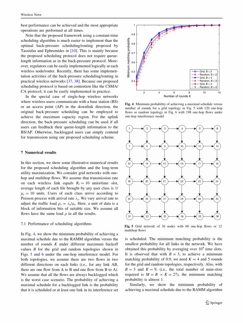
In Fig. 4, we show the minimum probability of achieving a
maximal schedule due to the RAMM algorithm versus the
number of rounds K under different maximum backoff
values B for the grid and random topologies shown in
Figs. 5 and 6 under the one-hop interference model. For
both topologies, we assume there are two flows in two
different directions on each links (i.e., for any link AB,
there are one flow from A to B and one flow from B to A).
We assume that all the flows are always backlogged which
is the worst case scenario. The probability of achieving a
maximal schedule for a backlogged link is the probability
that it is scheduled or at least one link in its interference set
is scheduled. The minimum matching probability is the
smallest probability for all links in the network. We have
obtained this probability by averaging over 104 time slots.
It is observed that with B = 3, to achieve a minimum
matching probability of 0.9, we need K = 4 and 5 rounds
for the grid and random topologies, respectively. Also, with
B = 3 and K = 9, (i.e., the total number of mini-slots
required is M = B 9 K = 27), the minimum matching
probability is almost 1.
Similarly, we show the minimum probability of
achieving a maximal schedule due to the RAMM algorithm
2 4 6 8 10 12
0.4
0.5
0.6
0.7
0.8
0.9
1
Number of rounds K
Min
imum
mat
chin
g pr
obab
ility
Grid, B = 2Random, B = 2Grid, B = 3Random, B = 3Grid, B = 4Random, B = 4
Fig. 4 Minimum probability of achieving a maximal schedule versus
number of rounds for a grid topology in Fig. 5 with 120 one-hop
flows or random topology in Fig. 6 with 198 one-hop flows under
one-hop interference model
Fig. 5 Grid network of 36 nodes with 60 one-hop flows or 12
multihop flows
Wireless Netw
123
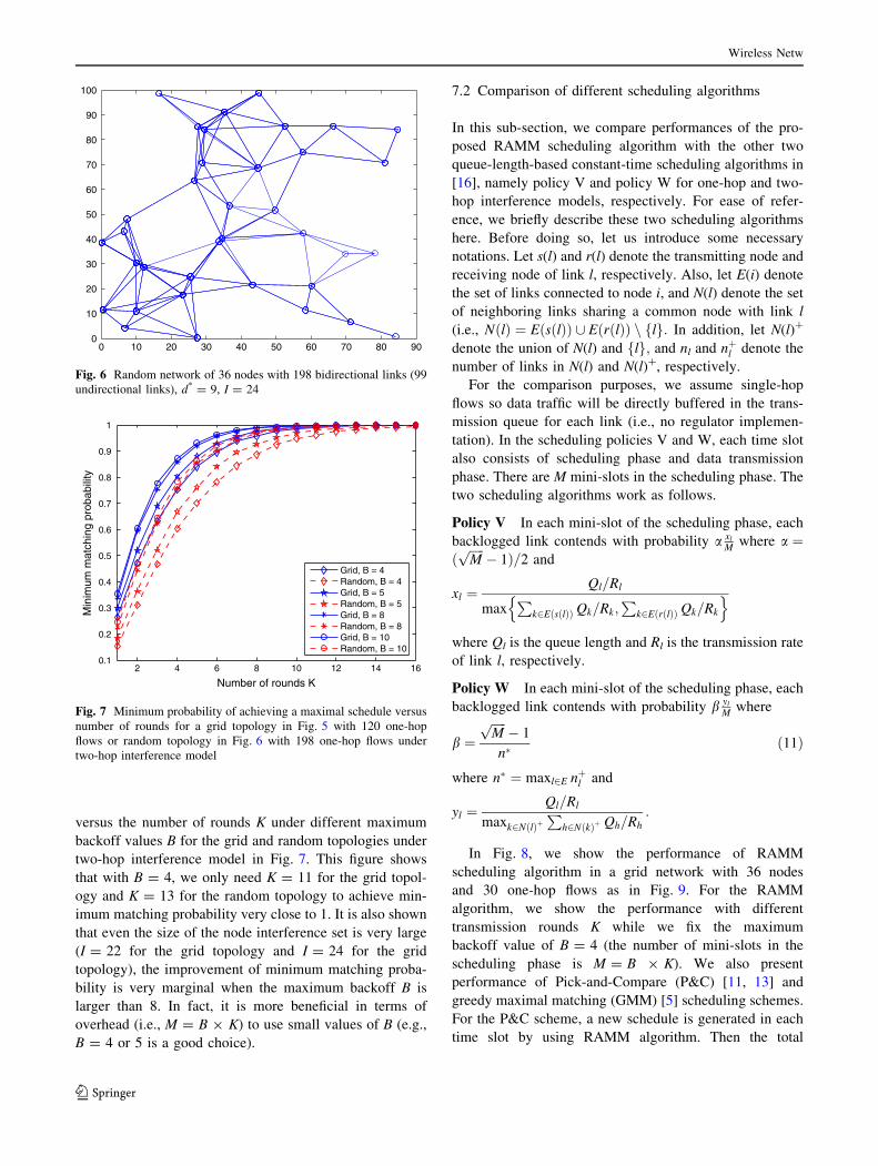
versus the number of rounds K under different maximum
backoff values B for the grid and random topologies under
two-hop interference model in Fig. 7. This figure shows
that with B = 4, we only need K = 11 for the grid topol-
ogy and K = 13 for the random topology to achieve min-
imum matching probability very close to 1. It is also shown
that even the size of the node interference set is very large
(I = 22 for the grid topology and I = 24 for the grid
topology), the improvement of minimum matching proba-
bility is very marginal when the maximum backoff B is
larger than 8. In fact, it is more beneficial in terms of
overhead (i.e., M = B 9 K) to use small values of B (e.g.,
B = 4 or 5 is a good choice).
7.2 Comparison of different scheduling algorithms
In this sub-section, we compare performances of the pro-
posed RAMM scheduling algorithm with the other two
queue-length-based constant-time scheduling algorithms in
[16], namely policy V and policy W for one-hop and two-
hop interference models, respectively. For ease of refer-
ence, we briefly describe these two scheduling algorithms
here. Before doing so, let us introduce some necessary
notations. Let s(l) and r(l) denote the transmitting node and
receiving node of link l, respectively. Also, let E(i) denote
the set of links connected to node i, and N(l) denote the set
of neighboring links sharing a common node with link l
(i.e., NðlÞ ¼ EðsðlÞÞ [ EðrðlÞÞ n lf g: In addition, let N(l)?
denote the union of N(l) and lf g; and nl and nþl denote the
number of links in N(l) and N(l)?, respectively.
For the comparison purposes, we assume single-hop
flows so data traffic will be directly buffered in the trans-
mission queue for each link (i.e., no regulator implemen-
tation). In the scheduling policies V and W, each time slot
also consists of scheduling phase and data transmission
phase. There are M mini-slots in the scheduling phase. The
two scheduling algorithms work as follows.
Policy V In each mini-slot of the scheduling phase, each
backlogged link contends with probability a xl
M where a ¼ðffiffiffiffiffiMp� 1Þ=2 and
xl ¼Ql=Rl
maxP
k2EðsðlÞÞ Qk=Rk;P
k2EðrðlÞÞ Qk=Rk
n o
where Ql is the queue length and Rl is the transmission rate
of link l, respectively.
Policy W In each mini-slot of the scheduling phase, each
backlogged link contends with probability b yl
M where
b ¼ffiffiffiffiffiMp� 1
n�ð11Þ
where n� ¼ maxl2E nþl and
yl ¼Ql=Rl
maxk2NðlÞþP
h2NðkÞþ Qh=Rh:
In Fig. 8, we show the performance of RAMM
scheduling algorithm in a grid network with 36 nodes
and 30 one-hop flows as in Fig. 9. For the RAMM
algorithm, we show the performance with different
transmission rounds K while we fix the maximum
backoff value of B = 4 (the number of mini-slots in the
scheduling phase is M = B 9 K). We also present
performance of Pick-and-Compare (P&C) [11, 13] and
greedy maximal matching (GMM) [5] scheduling schemes.
For the P&C scheme, a new schedule is generated in each
time slot by using RAMM algorithm. Then the total
0 10 20 30 40 50 60 70 80 900
10
20
30
40
50
60
70
80
90
100
Fig. 6 Random network of 36 nodes with 198 bidirectional links (99
undirectional links), d* = 9, I = 24
2 4 6 8 10 12 14 160.1
0.2
0.3
0.4
0.5
0.6
0.7
0.8
0.9
1
Number of rounds K
Min
imum
mat
chin
g pr
obab
ility
Grid, B = 4 Random, B = 4 Grid, B = 5Random, B = 5Grid, B = 8Random, B = 8Grid, B = 10Random, B = 10
Fig. 7 Minimum probability of achieving a maximal schedule versus
number of rounds for a grid topology in Fig. 5 with 120 one-hop
flows or random topology in Fig. 6 with 198 one-hop flows under
two-hop interference model
Wireless Netw
123
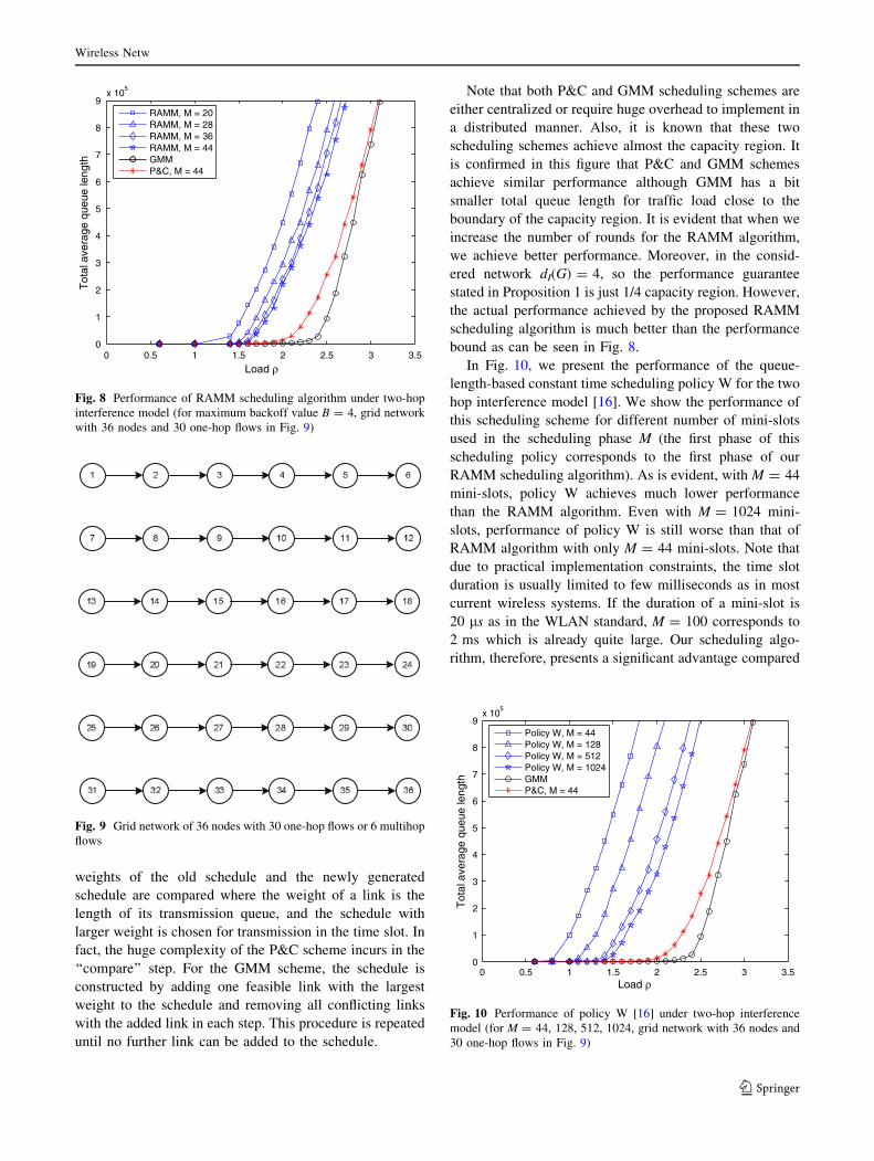
weights of the old schedule and the newly generated
schedule are compared where the weight of a link is the
length of its transmission queue, and the schedule with
larger weight is chosen for transmission in the time slot. In
fact, the huge complexity of the P&C scheme incurs in the
‘‘compare’’ step. For the GMM scheme, the schedule is
constructed by adding one feasible link with the largest
weight to the schedule and removing all conflicting links
with the added link in each step. This procedure is repeated
until no further link can be added to the schedule.
Note that both P&C and GMM scheduling schemes are
either centralized or require huge overhead to implement in
a distributed manner. Also, it is known that these two
scheduling schemes achieve almost the capacity region. It
is confirmed in this figure that P&C and GMM schemes
achieve similar performance although GMM has a bit
smaller total queue length for traffic load close to the
boundary of the capacity region. It is evident that when we
increase the number of rounds for the RAMM algorithm,
we achieve better performance. Moreover, in the consid-
ered network dI(G) = 4, so the performance guarantee
stated in Proposition 1 is just 1/4 capacity region. However,
the actual performance achieved by the proposed RAMM
scheduling algorithm is much better than the performance
bound as can be seen in Fig. 8.
In Fig. 10, we present the performance of the queue-
length-based constant time scheduling policy W for the two
hop interference model [16]. We show the performance of
this scheduling scheme for different number of mini-slots
used in the scheduling phase M (the first phase of this
scheduling policy corresponds to the first phase of our
RAMM scheduling algorithm). As is evident, with M = 44
mini-slots, policy W achieves much lower performance
than the RAMM algorithm. Even with M = 1024 mini-
slots, performance of policy W is still worse than that of
RAMM algorithm with only M = 44 mini-slots. Note that
due to practical implementation constraints, the time slot
duration is usually limited to few milliseconds as in most
current wireless systems. If the duration of a mini-slot is
20 ls as in the WLAN standard, M = 100 corresponds to
2 ms which is already quite large. Our scheduling algo-
rithm, therefore, presents a significant advantage compared
0 0.5 1 1.5 2 2.5 3 3.50
1
2
3
4
5
6
7
8
9x 10
5
Load ρ
Tot
al a
vera
ge q
ueue
leng
th
RAMM, M = 20RAMM, M = 28RAMM, M = 36RAMM, M = 44GMMP&C, M = 44
Fig. 8 Performance of RAMM scheduling algorithm under two-hop
interference model (for maximum backoff value B = 4, grid network
with 36 nodes and 30 one-hop flows in Fig. 9)
Fig. 9 Grid network of 36 nodes with 30 one-hop flows or 6 multihop
flows
0 0.5 1 1.5 2 2.5 3 3.50
1
2
3
4
5
6
7
8
9x 10
5
Load ρ
Tot
al a
vera
ge q
ueue
leng
th
Policy W, M = 44 Policy W, M = 128Policy W, M = 512Policy W, M = 1024GMMP&C, M = 44
Fig. 10 Performance of policy W [16] under two-hop interference
model (for M = 44, 128, 512, 1024, grid network with 36 nodes and
30 one-hop flows in Fig. 9)
Wireless Netw
123
to policy W because we cannot make the time slot interval
arbitrarily large in practice.
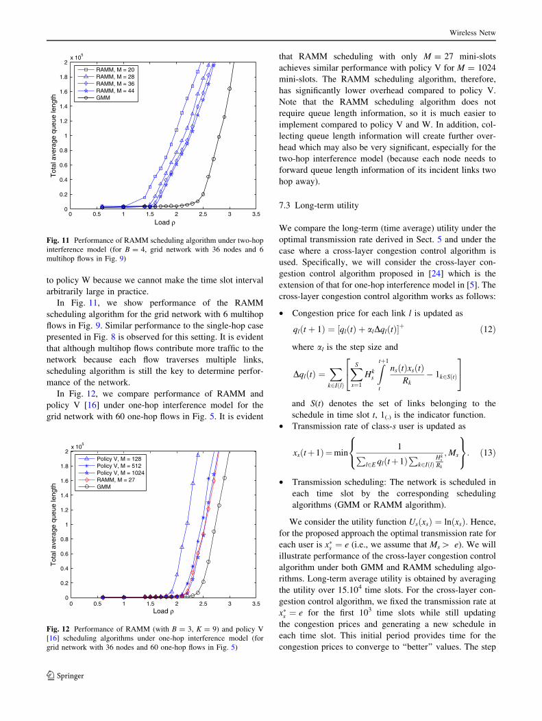
In Fig. 11, we show performance of the RAMM
scheduling algorithm for the grid network with 6 multihop
flows in Fig. 9. Similar performance to the single-hop case
presented in Fig. 8 is observed for this setting. It is evident
that although multihop flows contribute more traffic to the
network because each flow traverses multiple links,
scheduling algorithm is still the key to determine perfor-
mance of the network.
In Fig. 12, we compare performance of RAMM and
policy V [16] under one-hop interference model for the
grid network with 60 one-hop flows in Fig. 5. It is evident
that RAMM scheduling with only M = 27 mini-slots
achieves similar performance with policy V for M = 1024
mini-slots. The RAMM scheduling algorithm, therefore,
has significantly lower overhead compared to policy V.
Note that the RAMM scheduling algorithm does not
require queue length information, so it is much easier to
implement compared to policy V and W. In addition, col-
lecting queue length information will create further over-
head which may also be very significant, especially for the
two-hop interference model (because each node needs to
forward queue length information of its incident links two
hop away).
7.3 Long-term utility
We compare the long-term (time average) utility under the
optimal transmission rate derived in Sect. 5 and under the
case where a cross-layer congestion control algorithm is
used. Specifically, we will consider the cross-layer con-
gestion control algorithm proposed in [24] which is the
extension of that for one-hop interference model in [5]. The
cross-layer congestion control algorithm works as follows:
• Congestion price for each link l is updated as
qlðt þ 1Þ ¼ qlðtÞ þ alDqlðtÞ½ �þ ð12Þ
where al is the step size and
DqlðtÞ ¼X
k2IðlÞ
XS
s¼1
Hks
Ztþ1
t
nsðtÞxsðtÞRk
� 1k2SðtÞ
2
4
3
5
and S(t) denotes the set of links belonging to the
schedule in time slot t, 1(.) is the indicator function.
• Transmission rate of class-s user is updated as
xsðtþ1Þ¼min1
Pl2E qlðtþ1Þ
Pk2IðlÞ
Hks
Rk
;Ms
8<
:
9=
;: ð13Þ
• Transmission scheduling: The network is scheduled in
each time slot by the corresponding scheduling
algorithms (GMM or RAMM algorithm).
We consider the utility function UsðxsÞ ¼ lnðxsÞ: Hence,
for the proposed approach the optimal transmission rate for
each user is x�s ¼ e (i.e., we assume that Ms[ e). We will
illustrate performance of the cross-layer congestion control
algorithm under both GMM and RAMM scheduling algo-
rithms. Long-term average utility is obtained by averaging
the utility over 15.104 time slots. For the cross-layer con-
gestion control algorithm, we fixed the transmission rate at
x�s ¼ e for the first 103 time slots while still updating
the congestion prices and generating a new schedule in
each time slot. This initial period provides time for the
congestion prices to converge to ‘‘better’’ values. The step
0 0.5 1 1.5 2 2.5 3 3.50
0.2
0.4
0.6
0.8
1
1.2
1.4
1.6
1.8
2x 10
5
Load ρ
Tot
al a
vera
ge q
ueue
leng
th
RAMM, M = 20 RAMM, M = 28 RAMM, M = 36RAMM, M = 44GMM
Fig. 11 Performance of RAMM scheduling algorithm under two-hop
interference model (for B = 4, grid network with 36 nodes and 6
multihop flows in Fig. 9)
0 0.5 1 1.5 2 2.5 3 3.50
0.2
0.4
0.6
0.8
1
1.2
1.4
1.6
1.8
2x 10
5
Load ρ
Tot
al a
vera
ge q
ueue
leng
th
Policy V, M = 128Policy V, M = 512Policy V, M = 1024RAMM, M = 27GMM
Fig. 12 Performance of RAMM (with B = 3, K = 9) and policy V
[16] scheduling algorithms under one-hop interference model (for
grid network with 36 nodes and 60 one-hop flows in Fig. 5)
Wireless Netw
123

size is initialized as a = 0.1 and it is updated as
a ¼ max a=t; 10�3� �
:
We show the average utility achieved by the optimal
transmission rate and by the congestion control algorithm
in Figs. 13 and s14 for one-hop and two-hop interference
models, respectively. It is evident that the proposed
approach achieves higher average utility then those using
congestion control algorithm for all traffic load under both
interference models. In fact, the average utility with con-
gestion control decreases significantly when the traffic load
is close to the boundary of the region which can be stabi-
lized by the underlying scheduling algorithm. This obser-
vation confirms the argument that performing congestion
control is unnecessary if the network can be stabilized by
the underlying regulated scheduling algorithms.
8 Conclusions
We have investigated the network control problem using
constant-time scheduling under the k-hop interference
model. With flow dynamics consideration, we have shown
that the network can be stabilized by using a regulated
maximal scheduling policy if the offered load satisfies the
constraining bound. We have presented a constant-time and
distributed scheduling algorithm for a general k-hop inter-
ference model. The scheduling algorithm does not require
queue length information and has overhead not growing
with network size. Our proposed scheduling algorithm
achieves performance arbitrarily close to that of the regu-
lated maximal scheduling. Under the stability condition, we
have derived optimal transmission rates which achieve the
maximum long-term network utility. For the high load
regime, we have proposed a cross-layer congestion control
algorithm which can stabilize the network for any offered
load. Numerical results have shown that the proposed
scheduling algorithm achieves much better performance
than the existing constant-time scheduling algorithms in the
literature, and it has much better performance than its per-
formance guarantee. Also, performing congestion control
under low load condition actually degrades performance in
terms of long-term utility significantly compared to the case
where users transmit at the optimal transmission rate.
Appendix 1
Proof of Proposition 1
Let Qsl ðtÞ and Ql(t) be transmission queue lengths for class
s and for all user classes at link l in time slot t, respectively.
Similarly, let Psl ðtÞ and Pl(t) be regulator queue lengths for
class s and for all user classes at link l in time slot t,
respectively. Let us denote by bsl and as
l the previous link
and next link of link l on the route of class-s users. Also, let
Csl ðtÞ and Ds
l ðtÞ be the number of packets transmitted from
regulator and transmission queues in time slot t, respec-
tively. We have the following queue update equations
Qsl ðt þ 1Þ ¼ Qs
l ðtÞ � Dsl ðtÞ þ Cs
l ðtÞ ð14ÞPs
l ðt þ 1Þ ¼ Psl ðtÞ � Cs
l ðtÞ þ Dsbs
lðtÞ: ð15Þ
Thus, we have
Qsl ðt þ 1Þ þ Ps
aslðt þ 1Þ ¼ Qs
l ðtÞ þ Psas
lðtÞ þ Cs
l ðtÞ � Csas
lðtÞ:ð16Þ
0.5 1 1.5 2 2.5−200
−150
−100
−50
0
50
Load ρ
Ave
rage
util
ity
Congestion control, RAMMCongestion control, GMMOptimal transmission rate
Fig. 13 Average utility of the proposed optimal transmission rate and
with congestion control algorithm under one-hop interference model
(for grid network with 36 nodes and 12 multihop flows, GMM and
RAMM scheduling with B = 3, K = 9 in Fig. 5)
0.5 1 1.5 2 2.5−200
−150
−100
−50
0
50
Load ρ
Ave
rage
util
ity
Congestion control, RAMMCongestion control, GMMOptimal transmission rate
Fig. 14 Average utility of the proposed optimal transmission rate and
with congestion control algorithm under two-hop interference model
(for grid network with 36 nodes and 6 multihop flows, GMM and
RAMM scheduling with B = 4, K = 11 in Fig. 9)
Wireless Netw
123

We will use the following Lyapunov function for the
system
VðP~;Q~Þ ¼ V1ðQ~Þ þ nV2ðP~;Q~Þ ð17Þ
where
V1ðQ~Þ ¼X
l
QlðtÞRl
X
k2Il
QkðtÞRk
V2ðP~;Q~Þ ¼X
l
X
s
Psas
lþ Qs
l
� �2
:
In fact, this Lyapunov function was also used in [18].
Now, let us consider
V1ðQ~ðt þ 1ÞÞ � V1ðQ~ðtÞÞ
¼ 2X
l
QlðtÞRl
X
k2Il
ðQkðt þ 1Þ � QkðtÞÞRk
!
þX
l
ðQlðt þ 1Þ � QlðtÞÞRl
� �
�X
k2Il
X
s
ðQkðt þ 1Þ � QkðtÞÞRk
!ð18Þ
¼ 2X
l
QlðtÞRl
X
k2Il
X
s
ðCskðtÞ � Ds
kðtÞÞRk
!
þX
l
ðCsl ðtÞ � Ds
l ðtÞÞRl
X
k2Il
X
s
ðCskðtÞ � Ds
kðtÞÞRk
!:
Since the number of packets transmitted from regulator
and transmission queues in each time slot are bounded, the
second term in (18) can be bounded by a constant B1. Thus,
we have
E V1ðQ~ðtþ1ÞÞ�V1ðQ~ðtÞÞjP~ðtÞ;Q~ðtÞh i
�2EX
l
QlðtÞRl
X
k2Il
X
s
ðCskðtÞ�Ds
kðtÞÞRk
!jP~ðtÞ;Q~ðtÞ
" #þB1
�2EX
l:QlðtÞ�Rl
QlðtÞRl
X
k2Il
X
s
CskðtÞRk�X
k2Il
DkðtÞRk
!jP~ðtÞ;Q~ðtÞ
2
4
3
5
þB2:
Let L be the largest number of hops traversed by any
user class, we have
EX
l:QlðtÞ�Rl
QlðtÞRl
X
k2Il
X
s
CskðtÞRkjP~ðtÞ;Q~ðtÞ
24
35
�X
l:QlðtÞ�Rl
QlðtÞRl
X
k2Il
X
s
Hks qs þ L�
Rk: ð19Þ
Also, due to the definition of maximal scheduling
policy, we have
X
l:QlðtÞ�Rl
QlðtÞRl
X
k2Il
DkðtÞRk�
X
l:QlðtÞ�Rl
QlðtÞRl
: ð20Þ
For traffic load satisfying (5), we can find e and d small
enough such that
X
k2Il
XS
s¼1
Hks qs þ L�þ d
Rk� 1; 8l 2 E: ð21Þ
From (19), (20), (21), we have
E V1ðQ~ðtþ 1ÞÞ�V1ðQ~ðtÞÞjP~ðtÞ; Q~ðtÞh i
� � dX
l:QlðtÞ�Rl
QlðtÞRlþB2� � d
X
l
QlðtÞRlþB3:
ð22Þ
Now, using the procedure as in [18], we can obtain
E V2ðP~ðt þ 1Þ;Q~ðt þ 1ÞÞ � V2ðP~ðtÞ; Q~ðtÞÞjP~ðtÞ;Q~ðtÞh i
�X
l
X
s
RlQlðtÞ � gX
l
X
s
Psas
lðtÞ þ B4: ð23Þ
Combining the results in (22), (23), we have
E VðP~ðtþ1Þ;Q~ðtþ1ÞÞ�VðP~ðtÞ;Q~ðtÞÞjP~ðtÞ;Q~ðtÞh i
��X
l
X
s
dRl�nRl
� Qs
l ðtÞ�ngX
l
X
s
Psas
lðtÞþB5:
ð24Þ
We can choose n small enough such that dRl�nRl[0:
Thus, the drift will be negative if the regulator and/or
transmission queues become large enough. Therefore, the
stability result follows by using theorem 2 of [39]. Note
that the chosen Lyapunov function does not take regulator
queue on the first hop of each user class into account.
These regulator queues are, however, stable because their
output rate is qs ? e which is larger than the average input
load (i.e., qs).
Appendix 2
Proof of Proposition 2
Consider any link AB between node A and B. We will
find the probability that at least one link in the interfer-
ence set IAB is scheduled. This event will be denoted as
MAB in the sequel. As mentioned before, RAMM sched-
uling algorithm includes BP-SIM scheduling algorithm for
the one-hop (node exclusive) interference model proposed
in [17] as a special case. In the following we prove
Proposition 2 for k C 2. For the special case of k = 1, we
refer the readers to [17] for the proof and the corre-
sponding analysis. Note that the proof for the case k C 2
is very challenging and completely different from that for
Wireless Netw
123

the case k = 1 in [17] due to the more complicated
interference relationship.
We will illustrate some important definitions used in the
proof in Fig. 15. Let I0 be the set of nodes which is at most
k - 1 hops away from either A and B including A, B. For
the grid network and link AB shown in Fig. 15 under the
two-hop interference model, I0 ¼ A;B;C1; . . .;C6f g: Also,
the interference set for node C6 (i.e., IC6) consists of all
nodes in I0 and all ‘‘blank’’ nodes. Note that the notion of
node interference set is different from that of link inter-
ference set provided in definition I. Here, all nodes in IC6
are at most 3 hops away from C6. We observe that all links
incident to any nodes in I0 will belong to IAB because they
are within k hops from link AB. In the following, we will
find the lower bound for the probability of MAB by con-
sidering sub-cases in which there are i left nodes in the set
I0. For convenience, we will use I0 to denote both the set
itself and the corresponding number of nodes in I0. Let Li
be the event that there are i left nodes in the set I0. The
probability that at least one link in the interference set of
link AB is scheduled can be lower bounded as
Pm�XI0
i¼1
PrðMABjLiÞPrðLiÞ: ð25Þ
Recall that for any particular node A, there are at most I
nodes whose matching request can collide with that trans-
mitted from node A. Note that these I nodes will be at most
k ? 1 hops away from mode A. To find the lower bound for
the probability of MAB, we will assume the worst-case
scenario where each node has I interfering nodes. For
convenience, we also use IA to denote the set of these
interfering nodes whose transmissions can collide with that
from node A. We now consider the following cases.
There is only one left node in I0
We consider the following two sub-cases.
• If this left node is either A or B, then the left node will
have at least one neighbor which is a right node. This
case occurs with probability 2ð1=2ÞI0 : For ease of
reference, we will refer to this left node as node C (i.e.,
C is either A or B). Also, there are at most I - I0 nodes
whose matching requests can collide with that from
node C. To find the lower bound for Pr (MAB), we
assume that there are I - I0 such interfering nodes.
Now, suppose there are i left nodes among these I - I0
interfering nodes. The matching request transmitted by
node C will be successfully received if the backoff
values of these i left nodes are larger than that of node
C. Specifically, the matching request from node C will
be successfully received and the corresponding link
will be scheduled with a probability which is lower
bounded by
F1 ¼XI�I0
i¼0
I � I0
i
� �1
2
� �I�I0 1
B
XB
m¼1
1� m
B
� �i
where we have broken the event into sub-cases where
there are i left nodes among I - I0 interfering nodes and
these i left nodes have backoff values larger than that of
node C.
• If this left node is any node other than A and B then it
can be any node among (I0 - 2) nodes. Again, we refer
to this left node as node C. Note that all nodes which
are within one hop from A or B including A and B are
at most k ? 1 hops away from C so they all belong to
the interfering set IC. Let x be the total number of nodes
within one hop from A and B including A and B, then
there are at most I - x nodes whose matching requests
can collide with that from node C. This is because these
x nodes belong to I0 and they are all right nodes except
C if C is in I0. We will assume this worst-case scenario
to calculate the lower bound of the matching probabil-
ity in the following. Note that node C will have at least
one neighbor which is a right node because it is the only
left node in I0.
Again, suppose there are i left nodes among potential
interfering nodes in IC. The matching request transmitted
by node C will be successfully received if the backoff
values of these i left nodes are larger than that from
node C and the matching request from node C is
transmitted to a right node. Now, we consider the
Fig. 15 Interference set IC6under two-hop interference model
Wireless Netw
123

following two sub-cases. For the first case, if C is one of
x nodes (i.e., x one-hop neighbors of A or B) but not A
and B. Then, this case occurs with probability ðx� 2Þð1=2ÞI0 : In this case, the matching request from node C
will be successfully received and the corresponding link
will be scheduled with a probability which is lower
bounded by
F2 ¼XI�x�1
i¼0
I � x� 1
i
� �1
2
� �I�x1
B
XB
m¼1
1� m
B
� �i
where i is the number of left node. Also, in calculating the
lower bound for Pm we assume that C transmits its
matching request to a right node which is not an one-hop
neighbor of A or B. Hence, there are at most I - x - 1 left
nodes which can collide with the matching request from C.
For the second case, if C is not one of x nodes (i.e., x one-
hop neighbors of A or B). Then, this case occurs with
probability ðI0 � xÞð1=2ÞI0 : In this case, the matching
request from node C will be successfully received and the
corresponding link will be scheduled with a probability
which is lower bounded by
F3 ¼XI�x�2
i¼0
I � x� 2
i
� �1
2
� �I�x1
B
XB
m¼1
1� m
B
� �i
where in calculating the lower bound for Pm we assume
that C transmits its matching request to a right node which
is not an one-hop neighbor of A or B. Hence, there are at
most I - x - 2 left nodes which can collide with the
matching request from C.
There are two or more left nodes in I0
Suppose node C in the set I0 becomes left and wins the
contention. Then node C should have the smallest
backoff value among all the nodes whose matching
requests can collide with the matching request from C.
Also, node C should send the matching request to a node
which is a right one. For ease of reference, we will refer
to this right node as node D in the sequel. In general, D
can belong to set I0 or not. However, to find the lower
bound of Pm, we assume that D belongs to I0; therefore,
there are at most I0 - 2 other left nodes besides C and D
in I0.
As before, we assume the worst-case scenario where
there are I nodes whose transmissions can collide with that
of node C. Recall that all x nodes which are one-hop
neighbors of A or B belong to the set I. Similar to the
previous case, we consider the following two sub-cases.
For the first case, C is one of x nodes (i.e., x one-hop
neighbors of A or B). In this case the matching probability
can be lower bounded as
F4 ¼ xXI0�2
i¼1
XI�x�1
j¼0
I0 � 2
i
� �1
2
� �I0 I � x� 1
j
� �1
2
� �I�x
� 1
B
XB
m¼1
1� m
B
� �iþj
where i is the number of left nodes besides C and D in the
set I0. And j is the number of left nodes which belong to I
but are not one-hop neighbors of A or B (i.e., there is no
link between these nodes and A or B). We will denote this
set as I n x in the sequel. In general, D can belong to I n x or
not; however, to find the lower bound for Pm, we only
allow j takes values from 0 to I - x - 1. In addition, C can
be any node among x nodes so we have a factor of x before
the sum. Also, we require that all left nodes (i left nodes
belonging I0 and j left nodes belonging to I n x) achieve
larger backoff values than that of node C.
For the second case, C belong to the set I n x: In this
case, the matching probability can be lower bounded as
F5 ¼ I0 � xð ÞXI0�2
i¼1
XI�x�2
j¼0
I0 � 2
i
� �1
2
� �I0 I � x� 2
j
� �
� 1
2
� �I�x1
B
XB
m¼1
1� m
B
� �iþj
where C can be one of I0 - x nodes so we have the factor
I0 � xð Þ before the sum. Also, to calculate the lower bound
for the matching probability, we assume D always belong
to I n x; so j can be at most I - x - 2.
Substitute results of all considered cases into (25), the
matching probability is lower bounded by
Pm�P0m ¼ 2ð1=2ÞI0 F1 þ ðx� 2Þð1=2ÞI0 F2
þ ðI0 � xÞð1=2ÞI0 F3 þ F4 þ F5
ð26Þ
where F1, F2, F3, F4, and F5 are defined above.
From the lower bound of the matching probability P0m
derived above, we can calculate the lower bound of Pm for
any link AB as
p� ¼ minx;I0
P0m
where we find the minimum of P0m over all possible x and
I0. Note that possible values of x and I0 will be in the range
of [3, 2d*] and ½3; I�0 �; respectively. Here, x and I0 are at
least three for the network to be connected (i.e., A and B
should have at least one one-hop neighbor). It is observed
that p* is independent of the network size and depends only
on B, d*, I, I�0 : Now, we can choose K such that at least one
link in Il of a backlogged link l is scheduled with
probability greater than l after K rounds as follows:
K ¼ mink� 1
k : ð1� p�Þk� 1� ln o
: ð27Þ
Wireless Netw
123

Thus, we can choose K which is independent of network
size and only depends on B, d*, I, I�0 ; l such that
performance guarantee arbitrarily close to the
constraining bound can be achieved.
Example For the grid network and two-hop interference
model, we have I = 22, I0 = x can take values of 5, 6, 8.
With maximum backoff value B = 10, by using the anal-
ysis presented above, the minimum number of scheduling
rounds to achieve l = 0.9 is K = 60. In fact, this calcu-
lation is quite conservative because it considers the worst
case scenario. In practice, the size of interference sets
decreases quickly over scheduling rounds, so the required
value of K is much smaller.
Appendix 3
Proof of Proposition 4
The proof is similar to that of Proposition 1 (i.e., we use the
same Lyapunov function and proof procedure). In partic-
ular, we have a similar bound as in (19) as follows:
EX
l:QlðtÞ�Rl
QlðtÞRl
X
k2Il
X
s
CskðtÞRkjP~ðtÞ; Q~ðtÞ
24
35
�X
l:QlðtÞ�Rl
QlðtÞRl
X
k2Il
X
s
Hks x�s þ L�
Rk: ð28Þ
Due to the constraints of the optimization problem in
(10), we can find e and d small enough such that
X
k2Il
XS
s¼1
Hks x�s þ L�þ d
Rk� 1; 8l 2 E: ð29Þ
From (28) and (29), we have
E V1ðQ~ðt þ 1ÞÞ � V1ðQ~ðtÞÞjP~ðtÞ; Q~ðtÞh i
�
� dX
l:QlðtÞ�Rl
QlðtÞRlþ B6� � d
X
l
QlðtÞRlþ B7: ð30Þ
The remaining steps to obtain negative drift when
regulator and/or transmission queues become large enough
are the same as in the proof of Proposition 1.
References
1. Mo, J., & Walrand, J. (2000). Fair end-to-end window-based
congestion control. IEEE/ACM Transactions on Networking,8(5), 556–567.
2. Kelly, F. P., Maulloo, A., & Tan, D. (1998). Rate control in
communication networks: Shadow prices, proportional fairness
and stability. Journal of the Operation Research Society, 49,
237–252.
3. Low, S. H., & Lapsley, D. E. (1999). Optimal flow control, I:
Basic algorithm and convergence. IEEE/ACM Transactions onNetworking, 861–875.
4. Yaiche, H., Mazumdar, R., & Rosenberg, C. (2000). A game
theoretic framework for bandwidth allocation and pricing in
broadband networks. IEEE/ACM Transactions on Networking,8(5), 667–678.
5. Lin, X., & Shroff, N. B. (2006). The impact of imperfect
scheduling on cross-layer congestion control in wireless net-
works. IEEE/ACM Transactions on Networking, 14(2), 302–315.
6. Neely, M., Modiano, E., & Li, C. (2005). Fairness and optimal
stochastic control for heterogeneous networks. IEEE INFOCOM.
7. Hajek, B., & Sasaki, G. (1988). Link scheduling in polynomial
time. IEEE Transactions on Information Theory, 34, 910–917.
8. Bui, L., Eryilmaz, A., Srikant, R., & Wu, X. (2006). Joint
asynchronous congestion control and distributed scheduling for
multi-hop wireless networks. IEEE INFOCOM.
9. Sharma, G., Mazumdar, R., & Shroff, N. (2006). On the com-
plexity of scheduling in multihop wireless systems. IEEEMOBICOM.
10. Tassiulas, L., & Ephremides, A. (1992). Stability properties of
constrained queueing systems and scheduling policies for maxi-
mum throughput in multihop radio networks. IEEE Transactionson Automatic Control, 37(12), 1936–1948.
11. Tassiulas, L. (1998). Linear complexity algorithms for maximum
throughput in radio networks and input queued switches. IEEEINFOCOM.
12. Modiano, E., Shah, D., & Zussman, G. (2006). Maximizing
throughput in wireless networks via gossiping. ACMSIGMETRICS.
13. Eryilmaz, A., Ozdaglar, A., & Modiano, E. (2007). Polynomial
complexity algorithms for full utilization of multi-hop wireless
networks. IEEE INFOCOM.
14. Sanghavi, S., Bui, L., & Srikant, R. (2007). Distributed link
scheduling with constant overhead. ACM SIGMETRICS.
15. Lin, X., & Rasool, S. (2006). Constant-time distributed sched-
uling policies for ad hoc wireless networks. IEEE Conference onDecision and Control.
16. Joo, C., & Shroff, N. B. (2007). Performance of random access
scheduling schemes in multi-hop wireless networks. IEEEINFOCOM.
17. Gupta, A., Lin, X., & Srikant, R. (2007). Low-complexity dis-
tributed scheduling algorithms for wireless networks. IEEEINFOCOM.
18. Wu, X., Srikant, R., & Perkins, J. R. (2007). Scheduling efficiency
of distributed greedy scheduling algorithms in wireless networks.
IEEE Transactions on Mobile Computing, 6(6), 595–605.
19. Chaporkar, P., Kar, K., & Sarkar, S. (2005). Throughput guar-
antees through maximal scheduling in wireless networks. Aller-ton Conference on Communication, Control and Computing.
20. Kumar, P. R., & Seidman, T. I. (1990). Dynamic instabilities and
stabilization methods in distributed real-time scheduling of
manufacturing systems. IEEE Transactions on Automatic Con-trol, 35(3), 289–298.
21. Tassiulas, L. (1995). Adaptive back-pressure congestion control
based on local information. IEEE Transactions on AutomaticControl, 40(2), 236–250.
22. Humes, C., Jr. (1994). A regulator stabilization technique:
Kumar–Seidman revisited. IEEE Transactions on AutomaticControl, 39(1), 191–196.
23. Zhang, J., Zheng, D., & Chiang, M. (2007). The impact of sto-
chastic noisy feedback on distributed network utility maximiza-
tion. IEEE INFOCOM.
24. Sharma, G., Mazumdar, R., & Shroff, N. (2007). Joint congestion
control and distributed scheduling for throughput guarantees in
wireless networks. IEEE INFOCOM.
Wireless Netw
123

25. Le, L., & Mazumdar, R. R. (2008). Appropriate control of
wireless networks with flow level dynamics. CISS’08.
26. Zorzi, M., & Rao, R. R. (1994). Capture and retransmission
control in mobile radio. IEEE Journal on Selected Areas inCommunications, 12(8), 1289–1298.
27. Kim, J. H., & Lee, J. K. (1999). Capture effects of wireless
CSMA/CA protocols in Rayleigh and shadow fading channels.
IEEE Transactions on Vehicular Technology, 48(4), 1277–1286.
28. Hoang, D., & Iltis, R. A. (2008). Performance evaluation of
multi-hop CSMA/CA networks in fading environments. IEEETransactions on Communications, 56(1), 112–125.
29. Yang, X., & Vaidya, N. (2005). On physical carrier sensing in
wireless ad hoc networks. IEEE INFOCOM.
30. Cali, F., Conti, M., & Gregori, E. (2000). Dynamic tuning of the
IEEE 802.11 protocol to achieve a theoretical throughput limit.
IEEE/ACM Transactions on Networking, 8(6), 785–799.
31. Garetto, M., Salonidis, T., & Knightly, E. W. (2006). Modeling
per-flow throughput and capturing starvation in CSMA multi-hop
wireless networks. IEEE INFOCOM.
32. Xu, K., Gerla, M., & Bae, S. (2002). How effective is the IEEE
802.11 RTS/CTS handshake in ad hoc networks. IEEEGLOBECOM.
33. Jung, E. S., & Vaidya, N. H. (2005). A power control MAC
protocol for ad hoc networks. Wireless Networks, 11, 55–66.
34. Hass, Z. J., & Deng, J. (2002). Dual busy tone multiple access
(DBTMA)—A multiple access control scheme for ad hoc net-
works. IEEE Transactions on Communications, 50(6), 975–985.
35. Tobagi, F. A., & Kleinrock, L. (1975). Packet switching in radio
channels: Part II—The hidden terminal problem in carrier sense
multiple-access and the busy-tone solution. IEEE Transactions onCommunications, 23(12), 1417–1433.
36. Ma, K., Mazumdar, R. R., & Luo, J. (2008). On the performance
of primal/dual schemes for congestion control in networks with
dynamic flows. IEEE INFOCOM.
37. Sridharan, A., Moeller, S., & Krishnamachari, B. (2008). Making
distributed rate control using Lyapunov drifts a reality in wireless
sensor networks. WiOpt.38. Warrier, A., Janakiraman, S., & Rhee, I. (2009). DiffQ: Practical
differential backlog congestion control for wireless networks.
IEEE INFOCOM.
39. Neely, M., Modiano, E., & Rohrs, C. (2003) Power allocation and
routing in multibeam satellites with time-varying channels. IEEE/ACM Transactions on Networking, 11(1), 138–152.
Author Biographies
Long Bao Le received the B.E.
degree with highest distinction
from Ho Chi Minh City Uni-
versity of Technology in 1999,
the M.E. degree from Asian
Institute of Technology (AIT) in
2002, and the Ph.D. degree from
University of Manitoba in 2007.
He is currently a Postdoctoral
Research Associate at Massa-
chusetts Institute of Technol-
ogy. His current research
interests include cognitive
radio, cooperative diversity and
relay networks, and cross-layer
design for communication networks. He is a Member of the IEEE.
Ravi Mazumdar was born in
April 1955 in Bangalore, India.
He obtained the B.Tech. in
Electrical Engineering from the
Indian Institute of Technology,
Bombay, India in 1977, the
M.Sc. DIC in Control Systems
from Imperial College, London,
U.K. in 1978 and the Ph.D. in
Systems Science from the Uni-
versity of California, Los
Angeles, USA in 1983. He is
currently a University Research
Chair Professor of Electrical
and Computer Engineering at
the University of Waterloo, Waterloo, Canada and an Adjunct Pro-
fessor of ECE at Purdue University. He has served on the faculties of
Columbia University (NY, USA) and INRS-Telecommunications
(Montreal, Canada). He held a Chair in Operational Research and
Stochastic Systems in the Department of Mathematics at the Uni-
versity of Essex (Colchester, UK), and from 1999–2005 was Professor
of ECE at Purdue University (West Lafayette, USA). He has held
visiting positions and sabbatical leaves at UCLA, the University of
Twente (Netherlands), the Indian Institute of Science (Bangalore);
and the Ecole Nationale Superieure des Telecommunications (Paris).
He is a Fellow of the IEEE and the Royal Statistical Society. He is a
member of the working groups WG6.3 and 7.1 of the IFIP and a
member of SIAM and the IMS. He is a recipient of the IEEE IN-
FOCOM 2006 Best Paper Award and was runner-up for the Best
Paper at INFOCOM 1998. His research interests are in applied
probability, stochastic analysis, optimization, and game theory with
applications to wireless and wireline networks, traffic engineering,
filtering theory, and mathematical finance.
Wireless Netw
123