Control of thermal runaway—some mathematical insights

lnlcrnational Journalof

HEAT ati MASS TRANSFER

International Journal of Heat and Mass Transfer 41 (1998) 2979-2990

Control of thermal runaway-some mathematical insights James GeeP*, John Fillob

a Department of Syskws Science and Industrial Engineering, Watson School of Engineering, SUNY, Binghamton, NY 13902, USA b Associate Dean& Research and External Affairs, Watson School of Engineering, SUNY, Binghamton, NY 13902, USA

Received 12 May 1997 ; in final form 8 December 1997

Abstract

The model problem of a heat generating fluid flowing through a finite length pipe is investigated analytically to study means of controlling the onset and development of thermal runaway. The heat source Q within the fluid is modeled as a linear function of the temperature and it is shown that, when Q is sufficiently large, the temperature will, in general, grow exponentially in time, i.e., thermal runaway will occur. However, even when this is the case, it is shown that thermal runaway can be prevented by imposing certain conditions on : (1) the initial temperature distribution ; (2) the time dependent temperature of the ambient fluid surrounding the pipe; or (3) the time dependent boundary conditions. The results are discussed and are illustrated by several examples. 0 1998 Elsevier Science Ltd. All rights reserved.

Nomenclature

A a

; h k L m P

4 Q

cross-sectional arca non-dimensional amplitude specific heat eigenfunction heat transfer coefficient heat conduction coefficient length of pipe heat source coefficient periphery of pipe heat source coeffic:lent internal heat generation per unit volume

Q exp exponential moldel of internal heat generation per unit volume Qllnear linear model of internal heat generation per unit volume T time TO initial time t nondimensional time, k(T- TJ/pcL’ u nondimensional temperature, (0 - &J/O, Uo(t), U,(t) specified boundary temperatures V constant velocity of the fluid in the pipe X distance from pipe inlet x nondimensional distance, X/L.

* Corresponding author.

0017-9310/98 $19.00 0 1998 Elsevier Science Ltd. All rights reserved P11:s0017-9310(98:100009-x

Greek symbols c( one-half the Peclet number, pcLV/(2k)

B PI-B* j?1 heat source parameter, mL’/k bz convective sink parameter, hPL2/kA

Y ?I+?2 y, external heat source parameter, qL2/k0, yz ambient temperature parameter, hPL*(B, - Q,)/(kA&)

coefficient in the model Qexp fluid temperature ambient temperature inlet temperature exit temperature constant reference temperature

eigenvalue density initial temperature nondimensional initial temperature, [m(x) -&l/O, nondimensional frequency.

1. Introduction

The variation and distribution of temperature within a solid or fluid material, in which heat is being generated at a rate which depends on the temperature, is a subject of considerable technical importance. This situation com-

2980 J. Geer, J. FiDojInt. J. Heat Transfer 41 (1998) 2979-2990

monly arises when the local temperature interacts with the mechanism causing the generation of heat. Examples include internal chemical reactions in a shock-com- pressed material [l], electrical energy dissipation within solid dielectrics in regions where the electrical resistance changes with temperature [2], electrochemical reactions producing heat in battery systems [3], heating of ceramics with microwave energy [4], heat generation due to the nonradiative recombination of minority carriers in semiconductor lasers [5], and the chemical reaction carried out in a fixed-bed flow reactor [6]. These examples, as well as many others, have in common the feature that heat is being generated at a rate which depends upon the temperature. In such cases, a major topic of interest is the prediction of the temperature distribution and the condition which causes the temperature to increase in an unbounded fashion, i.e., the determination of the conditions that can cause thermal runaway.

The determination of conditions which set limits for the temperature to remain bounded and approach a steady state is of technical interest. Thermal runaway can be interpreted as the consequence of a temperature dependence of sufficient magnitude that the temperature rise necessary to cause the generated energy to be conducted to a surface and then removed by convection causes an increase in the generation rate, which is too large to be conducted and convected away. In [7], an interesting result occurs in which thermal runaway can be induced, or prevented, by varying the ambient temperature. The suggestion is that, if the occurrence or prevention of thermal runaway can be affected by variation of the ambient temperature, then perhaps thermal runaway can be controlled through other external means, e.g., by the initial conditions and/or the boundary conditions of the problem. It is this issue that is addressed in this paper. Although we restrict our attention to a model problem concerning a heat generating fluid flowing through a pipe, we feel that several of the basic ideas we shall discuss are applicable to more general physical situations. For example, setting the fluid velocity equal to zero, we recover temperature solutions applicable to solids [2, 8-101. Thermal runaway is discussed in these references, but our results, presented below, include additional findings that are not discussed or recognized in the references cited. In addition, the systematic analysis and discussion of the model problem we shall present does not appear to have been addressed in the literature.

In Section 2, we formulate the model problem we wish to consider and then, in Section 3, present the analytical solution for the case of constant ambient temperature. This solution is analyzed, and it is shown how thermal runaway can be prevented by requiring the initial condition to satisfy certain conditions. In Section 4, the analytical solution for the case of a general, time varying, ambient temperature is presented and two special cases are analyzed in detail. Again, it is shown how thermal

runaway can be controlled by requiring the ambient temperature to satisfy a certain set of conditions. In Section 5, we consider the case of time dependent boundary conditions. The analytical solution for this case is presented and analyzed, and the conditions necessary to control thermal runaway are presented. In Sections 3-5, the results are illustrated with several examples. We discuss our results in Section 6.

2. Model problem-Transient beat convection in a pipe

We consider a heat generating fluid flowing through a pipe of length L which transfers heat through its surface with coefficient h to an ambient fluid at temperature 6 = B,(T), where T denotes time (see Fig. 1). The heat generated in a small control volume of the fluid is assumed to be a linear function of the average temperature 0 of the volume, while the fluid velocity V is assumed to be uniform over the cross-section A of the pipe and constant along the length of the pipe. The temperature B,, at the entrance to the pipe and the temperature QL at the exit of the pipe are specified and are assumed to be constant over the cross-section of the pipe. The thermal conductivity k is assumed to be a constant. The initial temperature of the fluid is also specified. We wish to determine the transient, radially lumped, and axially distributed temperature ~9 of the fluid (i.e., the temperature is assumed to be uniform over a given cross- section and is a function only of time and the distance X along the pipe).

The balance of thermal energy applied to a radially lumped and axially differential control volume yields

Xi ;12A

pcyT = kg +q+m(Q-8,)

- 7. [U--B,(T)]--pcYg for 0 < X < L, T > T,,, with the boundary conditions

19 = B0 at X= 0, 0 = L$, at X = L

and the initial condition 0 = (D(x), when T = To. Here p and c are the (constant) density and specific heat of the fluid, respectively. The model we shall use of the heat source per unit volume is a simple linear function of temperature, namely, q+m(B-O,), where q and m are specified constants. Here q can be interpreted as the exter- nally imposed heating rate per unit volume at temperature f?,,, while m(O-0,) models the (linear) variation of the rate with the temperature difference 0-B,,. (We shall discuss this model further in Section 6.) The coordinate X is measured from the inlet of the pipe in the downstream direction, P is the periphery of the pipe, and Q(x) is the initial temperature distribution of the fluid in the pipe.

J. Geer, J. Fillojlnt. J. Heat Transfer 41 (1998) 2979-2990 2981

.L------+ Fig. 1. A sketch of the geometry of the model problem of flow through a pipe of finite length, with an indication of the coordinate system.

To simplify notation, we let 0, be any convenient, non- zero constant reference temperature and define the nondimensional quantities

hPL2 B,(T) - 6+, Y2(0 =--g-

eL-00

Qr ’ U’=e,’

Then, in terms of these variables, the nondimensional temperature u satisfies

au ah at a2

-2or~+/h+y(t), o<x< 1, t > 0, (1)

u = 0, at x = 0, U == u,,

atx= 1, and u = 4(x), when t = 0. (2)

We note that /I, and y, are proportional to the heat generation coefficients m and 4, respectively, and are each inversely proportional to k. Also, f12 is proportional to h, while y2 is proportional to both h and the temperature difference f3,( T) - B,,. The parameter 2a is the Peclet number of the flow, and is a measure of the ratio of the axial enthalpy flow and the axial conduction.

3. Constant ambient temperature

We consider first the case when the ambient temperature 0, is a constant. Then y is a constant and the solution for u can be expressed as

4% 4 = UI ‘Xf 2 gk(ofkw, k=,

gk(t) = f + (g,(O)-- $>ed’.

&(x) = e”“sin(knx), 1, = k2z2 +a2 -B,

Qk = (Y--w)A,+Bu,&

g,(O) = 2 I

1 4(x)eeUXsin(kax)dx-u, -B,

0

A, = $$[I-(-l)‘ee”], k

Bk E*

@k +8)’

[(-l)k+‘ee”(2cc+fi+Lk)+2a]. (3)

Here (fk(x)} are the eigenfunctions associated with equation (1) and II, are the associated eigenvalues.

We now make some observations about our solution u(x, t). To do this, we find it convenient to consider two cases, corresponding to whether or not all of the eigenvalues (1,) are positive.

Case 1: All of the eigenvalues ik are positive. In this case, u will approach a steady state solution,

ups(x), at t -+ co. Here u,, is given by equation (3) with gk(t) replaced by the constant Qk/nk, and can also be expressed as

u,,(x) = B sil(o,) { (Bu, + y)e”+ ‘) sin(m)

+ ye""sin [o(l -x)] --y sin(w)} (4)

where w = JB-‘. LX From the definition of ik in equation (3) we see that all of the eigenvalues will be positive as long as /I < a’+ rr2. (See Fig. 2 and also Section 6, where this condition is discussed further.)

2982 J. Geer, J. Fillollnt. J. Heat Transfer 41 (1998) 2979-2990

0 K=O

-7.5 -5 -2.5 0 2.5 5 7.5

(I

Fig.2.Aplotofthecurves1,=k2r?+a*-_=O,fork= 1,2,3, with an indication of the regions of the Q-plane where there are exactly K negative eigenvalues, for K = 0, 1, 2, and 3.

To illustrate this case, we let u, = 1, a = 1, /3 = 6, and y = 0, which implies that ;Lk > 0 for all k > 1. We then let q(x) = - 1 and plot u(x, 1) at several values of t in Fig. 3(a). The solution u,,(x) is also plotted.

Case 2 : One or more of the eigenvalues are negative. This case will occur whenever /l > CX’ + k2x2, for some

integer k. More specifically, suppose that 1, < 0 for l<k<K,whilei,>O,fork>K+l,whereKissome positive integer. (Here K is just the number of negative eigenvalues for the problem.) In this case, u will, in general, grow exponentially as t -+ co, i.e., thermal runaway will occur, and no steady state solution will be attained. (This is the situation discussed in [2, 81 and [lo] for the case when tl = 0.) This is due to the presence of the term in gk(t) proportional to e-‘k’, for 1 < k < K. However, even in this case, it is still possible, under certain circumstances, for the steady state solution u,, to be attained. To see this, we note that the solution (3) will still approach the steady state solution u,, if the coefficient of e-‘k’ in gk(t) vanishes for 1 < k < K, i.e., if

gk(0) - + = 0, 1 < k < K. k

Using the definitions in equation (3), these requirements can be expressed as conditions on the form of the initial condition 4(x) as

sin(krrx) dx = ck, (5)

for 1 < k < K. As an example of these results, we consider the case

whenK=l,Thus,1,<Oand1,>Ofork>K+1=2. Then, the constant initial temperature

satisfies the condition (5) for k = 1. Here c, is defined by equation (6) with k = 1. In Figs. 3(b)-(d) we have plotted u(x, t) at various times for u, = 1, a = 1, b = 12, and y = 0 (which implies that K = 1, with 1, = rr2 - 11 < 0) and for 4(x) = 6 * @, with 6 = 1, 0.9, and 1.1, respectively. In this case, thermal runaway will occur for any value of 6 # 1, but it can be avoided if 6 = 1, i.e., if

4(x) 5 4:. Other initial temperature profiles satisfying the con-

dition (5) can be constructed in a straightforward manner. In particular, when K 2 1, it is possible to find rather general families of initial temperature distributions which satisfy the conditions (5) for 1 < k < K, provided that each member of the family contains at least K arbitrary constants. For example, one such family is the set of all polynomials of degree at least K- 1. For example, when K = 2 the initial temperature

d;(x) = f$(O) +#“X, (8)

@“’ = 2 c,B,-c,B,

#I) = 2 c,A, -CIA, A,B,-A,B,’ A,BZ-A2B, ’ (9)

where Ak and B, are defined in equation (3), satisfies conditions (5) fork = 1 and k = 2.

More generally, we can construct an initial temperature profile 4*(x) that satisfies conditions (5) starting with any piece-wise continuous function $(x). In particular, it is straightforward to verify that

4*(x) = It/(x>+ i akeZX sin(knx), k=l

ak = 2 ck - ( I

: $(x)ePX sin(knx) dx), k= 1,2 ,..., K,

(10)

satisfies the conditions (5), where ck is defined in equation

(6).

4. Time dependent ambient temperature

We now generalize the problem of the previous section and allow 6, to be an arbitrary, specified function of time. (In [7], thermal runaway is induced by increasing the ambient temperature as a linear function of time.) Letting

J. Geer, J. Fillollnt. J. Heat Transfer 41 (1998) 2979-2990 2983

T------ (a)

I

0.5

s

‘:;& Me

. /

50. z--e-- / / / ,I:’

s ,;‘ , / 1: \’ \ \ \ . . / ,I:

-0.5 ‘\ ’ \ ’

- . , ’ -_ I / ,’

’ ‘1 / II

-1 +f-1‘ / / .I’

-----z= -

t -isL------

0 0.2 0.4 0.6 0.8 ’

X

I

w

L

(b)

1 I

-41 I 0 0.2 0.4 0.6 0.8 1

(d)

X

\ ‘-0 /

-8. \ / \ /

1, -10

I -al------ _’ I I, a 0 0.2 0.4 0.6

__ u.u 1 0 0.2 0.4

__ 0.6

_^ U.M 1

X X

Fig. 3. The transient temperature distribution u(x, t) (dashed lines) for several values of t, for: (a) CI = 1, /3 = 6, and y = 0 (which implies that all of the eigenvalues are positive) ; the constant initial temperature and the final steady state solution u,, are indicated by solid lines; (b) G( = 1, fl = 12, and y = 0 (which implies that K = 1, i.e. A, < 0 and Lk > 0 for k 2 2) ; the critical constant initial temperature q$ and the final steady state solution u,, are indicated by solid lines ; (c) same parameters as (b), except that the constant initial temperature is 0.9 s cp$, which is indicated by a solid line, while the critical constant initial temperature cp$ is indicated by a dotted line ; in this case, no steady state solution is attained and the solution grows exponentially ; (d) same parameters as (b), except that the constant initial temperature is 1.1 * cp$, which is indicated by a solid line, while the critical constant initial temperature q$ is indicated by a dotted line ; as in (~11, the magnitude of the solution grows exponentially.

2984 J. Geer, J. FillojInt. J. Heat Transfer 41 (1998) 2979-2990

y = y(t) be a (specified) function of time, the solution for u can be written as

gk(t) = Ak s ’ y(r)eik(Tp’) dz. (12) II

Here Qk is just Qk, defined in equation (3), with y = 0, while gk(0) and&(x) are defined in equation (3). For this case, the behavior of each g,(t), and, hence, the behavior of u(x, t), as t -+ co, will depend on the behavior of &k(t) as t + co. Instead of stating general conditions under which c&(t) will behave in some particular manner, we find it more instructive to look at two specific examples.

4.1. Ambient temperature is apolynomialfinction of time

First, we let y(t) be a polynomial function of time and write

y(t) = 2 y’“’ et”, n=O

where N is a nonnegative integer and each y(“) is a constant. Using equation (12), for this case we find

(13)

where Qp’ is just Qk, defined in equation (3), withy = y(O).

Case 1: All of the eigenvalues I, are positive. Then u will approach the solution

N

24, (x, t) = c v(“)(x) * t” )

n=o

as t -+ co. Here v(“)(x) is just the coefficient of r in equation (11) when gk(t) is replaced by the right side of equation (13), with the term proportional to e&k’ set equal to zero. In this case, the magnitude of u will eventually grow as a polynomial function of time. For example, for N = 1, y(t) zz y(O) + y(‘) * t and we find that v’“‘(x) is given by equation (11) with gk(t) replaced by the constant (Q~“)/&-A,$‘)/L:), while v(‘)(x) is given by equation (11) with u, = 0 and gk(t) replaced by the constant (&+“l&).

Case 2 : One or more of the eigenvalues are negative. In this case, u will, in general, grow exponentially as

t --f 00, i.e., thermal run-away will occur. However, even

in this case, it is possible, under certain circumstances, for the solution to grow as (only) a polynomial function of time and not, in particular, to grow exponentially with time. To see this, suppose that Ak < 0 for 1 < k < K, while Ak > 0, for k > K+ 1. Then the solution (11) will not grow exponentially in time if the coefficient of e-“k’ in gk(t) vanishes for 1 < k < K, i.e., if

gk(0)- if! +Ak 2 (- ‘)“++$‘” = 0,

1;” k= 1,2 ,..., K.

n=l

(14)

The conditions (14) are a system of K linear constraints that must be satisfied by the N parameters (coefficeints) {y(“‘}. For example, if we set N = K, they become a system of K linear algebraic equations for the parameters {y”‘, . . . ) ycx?}. Thus, if the conditions (14) are satisfied, u will again approach the solution u, as t -+ 00.

To illustrate this possibility, in Figs. 4(a) and (b) we have plotted u(x, t) as a function of time for several values of x, for 4(x) = 0, u, = 1, tl = 1, /l = 13, N = 1, and y(O) = 1. (Here K = 1, since A, < 0 and I, > 0 for k > 2.) In Fig. 4(a), we have set

Y (‘1 = +I)* S _ $,(()_Q(“‘:i,); (15) I

as determined from equation (14) with N = K = 1. In this case, although there is a negative eigenvalue, the solution grows as (only) a linear function of time. In Fig. 4(b), we have used the same parameter values as in Fig. 4(a), except that y(l) = 0.95 * y(‘)*. In this case, the solution eventually grows exponentially with time.

4.2. Ambient temperature is a periodic junction of time

Second, we let y(t) be of the form

y(t) = a0 + 2 a, sin(q), j=l

(16)

where each aj and CD, is an arbitrary constant. For this case, we find

gk(t) = y + ( gk(0)- $? +A, f a e-“G k ,=Ii,2+w~~ >

+Ak f aj* j= 1

where Qp) is now given by Qk in equation (3), with y = a,.

Case I : All of the eigenvalues 1, are positive. In this case, u will approach the bounded, time varying

solution 6(x, t), given from equations (11) and (17) by

J. Geer, J. Fillo/Int. J. Heat Transfer 41 (1998) 2979-2990 2985

(4

2.5

(‘4

0 1 2 3 4 5'

t

Fig. 4. The transient temperature distribution u(x, f), when the ambient temperature is a linear function of time [(a) and (b)] and when the ambient temperature is a sinusoidal function of time (c), plotted as a function of t for x = l/4 (dotted line), x = l/2 (solid line), andx=3/4(dashedline).In(a)and(b),u, = l,+(x)=O,c1= 1,/I= 13,andy (‘) = 1 (which implies that K = 1, i.e., A, < 0 and I, > 0 fork > 2). In (a), y(l) = y(r)* [f rom equation (15)] and the magnitude of u eventually grows linearly with time; in (b), y”’ = 0.95 *y(r)* and the magnitude of u (eventually grows exponentially with time. In (c), ur = 1, d(x) = 0, c( = 1, 1 = rr2+2 (which implies that K = 1, i.e., I, = - 1 and E., > 0 for k > 2), and a, = 0, while a, and w1 are determined from equation (22) with 6 = l/2. In this case, u eventually approaches the (bounded) periodic solution zi(x, t), as t + co.

1, sin(wjt) -wj cos(w,t)

Case 2 : One or more of the eigenvalues are negative.

Let&<O,for 1 <k<K,with&>O,fork2K+l. In this case, u will, in general, grow exp.onentially as t -+ co, i.e., thermal runaway will occur. However, even in this case, it is still possible for u to approach 2(x, t), as

2986 J. Geer, J. FillojInt. J. Heat Transfer 41 (1998) 2979-2990

t -+ co, if the coefficient of e-‘k’ in gL(t) vanishes for 1 < k ,< K, i.e., if

0, k=1,2 ,..., K.

(18) These conditions can, in turn, be satisfied by properly choosing the parameters N, {u,}, and {w,}. For example, setting N = K and letting each W, be a convenient, non- zero constant, we can write the conditions (18) as

pLu,=- gk(0)-Qi”)/~~k ,=I g+w,2 A,

, k=1,2 ,..., K,

(19)

which is just a system of K linear, algebraic equations for the K amplitudes (u,}. Alternatively, if we specify the amplitudes {u,}, then equation (19) are a system of (nonlinear) equations for the K frequencies {o,).

To illustrate these results, we set d(x) = 0, u, = 1, a=l,~=~2+2,anda,,=0,whichimpliesthatK=l, with 2, = - 1 and & > 0, for k > 2. Then equation (19) becomes

UlWl 1+7?

1+w: l+e (20)

This equation can be satisfied by letting w, be any convenient, non-zero constant and then solving for a, as

1-w: I+712 al=-P*P l+e ’ WI zo, arbitrary. (21)

ml

Alternatively, we can set a, = -2( I+ n*)/[6(1 +e)], where 0 < 161 < 1, and then solve equation (20) for w, as

w, = l&-$X 2(1 +7c2)

6 ’ a’ = - 6(1$-e) ’

where0 < 161 < 1. (22)

In Fig. 4(c) we have plotted u(x, t) as a function oft for several values of x, with w, and a, determined by equation

(22) with 6 = l/2, i.e., 0, = 2+$ and a, = -4(l +n2)/(l+e) e -11.69. In this case, u -+ Q(x, t), as t + co.

5. Time dependent boundary conditions

In many practical problems, time dependent boundary conditions play an important role. For example, they are of importance in cases involving the flow and heat transfer associated with vibrating components of a variety of mechanical systems, such as reciprocating engines. Thus, we now generalize our model problem by allowing the boundary conditions to vary with time. For simplicity, let 0, (and, hence, 7) be a constant. Thus, in nondimensional form, we consider the problem

au a2u -= - -2Kg +pu+;‘, at &’ -+*

O<x<l, t>o, (23)

u = Uo(t), at x = 0, u = U,(t), at x = 1

and u = 4(x) when t = 0. (24)

Here Uo(t) and U,(t) are specified (smooth) functions of time.

For this case, the solution for u can be expressed as

n(-x, t) = (1 --y)U,,(t)+-x-l/, (t)+ i gk(t).fk(-x), (25) i=I

where {fk(x)} are defined in equation (3), and gk(t) is now given by

gk(t) = e-Q gk(0)

f-h $eQ- 1) + U,(O) - Uo(t)eQ

+(p+2a+j”k)G0,k(t)-21G,,k(t) 1 +(Uo(t)-U,(t))e’~‘-Uo(0)+u,(O)l , I (26)

gk(0) = 2 i

’ eP”4(x) sin(knx) dx 0

-AkuO(O)-Bk[U,(O)-u0(0)1.

Here we have defined

C,.k(Q = s

U,(z)e’kT dz, j = 1,2, (27) 0

for k = 1,2,. , while Akr A,, and B, are defined in equation (3).

As an example of these results, we consider the special case when

U,(t) = i u, sin(wjt), U,(r) = 1 + r/o(t), (28) ,= I

where the amplitudes {a,} and the frequencies {wj} are arbitrary constants, and N is an arbitrary positive integer. Using equations (26)-(28), we find

gktt)

u,(P+3’k)W, cos(w,t) 2a-y _

> 1 - /1 , .k

(29)

where

J. Geer, J. FillolInt. J. Heat Transfer 41 (1998) 2979-2990 2987

s 1

gkm = 2 eeUX$(x:l sin(knx) dx-B,. (30) 0

Case 1: All of the eigenvalues lk are positive. Then u will approach a ‘steady’, i.e., bounded, solution

as t -+ co, given by equation (25) with g,,(t) defined by the right side of equation (29), with the term e-i’ set equal to zero.

Case 2 : One or more qf the eigenvalues are negative. In this case, u will, in general, grow exponentially as

t + co, i.e., thermal runaway will occur, and no bounded solution will be attained. However, even in this case, it is again possible, u:nder certain circumstances, for a ‘steady’, or bounded, time varying, solution to be attained. To see this, suppose that 1, < 0 for 1 < k < K, while 1, > 0, for k > K+ 1. Then the solution (25) will approach a steady solution, if the coefficient of e-‘k’ in gk(t) in equation (29) vanishes for 1 d k < K, i.e., if

k=1,2 ,..., K. (31)

These equations can be satisfied, for example, by setting N = K, setting each CD\ to a convenient constant, and then solving the resulting K linear equations (31) for the K unknown amplitudes a,, . . . , uK. Alternatively, equation (31) can be satisfied by selecting convenient values for the amplitudes {aj} and then solving the resulting nonlinear equations for the frequencies {wj} (provided, of course, that such solutions exist).

As an application of these results, we again consider the case when K = 1 ((i.e., when there is just one negative eigenvalue) and we set N = 1 in equation (31). Then the condition on a, and CD, becomes

SIW~B, +A, ( aI @+&h 2c(-y - ___ =O.

I 3,: +uJ: + 1, > (32)

If we assume that the initial condition for u is specified, then g, (0) is known [see equation (30)] and equation (32) can be solved for either a, or w1 in terms of the other parameter. As an example of this case, we let 4(x) = 0, CC= 1, p=7?+2, and y =O. Then K= 1, with 1, = n*+c?--_B = - 1, and 1, > 0 fork > 2. In this case, equation (32) reduces, to

alwl

1+0:

1

l+e’ (33)

For an arbitrary value of w, # 0, we can solve equation (33) for a, and find

1+w: “=--w,

011 # 0, arbitrary. (34)

Alternatively, we can set a, = - (Z/S)[l/(l +e)], where

6 is any real number satisfying 0 < 161 < 1, and solve equation (33) for w, to find

w, = 1+-t

6 ’

with a,=-;*&. 0<]61<1. (35)

Thus, with a, and w, determined by either equation (34) or equation (35) the condition (32) is satisfied for this case, and, hence, u will approach a bounded (periodic) solution as t + co.

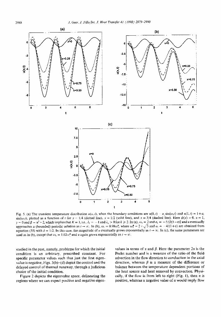
To illustrate these results, in Fig. 5(a) we have plotted u as a function of t for several values of x, with w, = 2 and a, determined from equation (34) as -5/[2(1+e)] A -0.672. If we set 6 = l/2 in equation (35) and then set w, = 2+$ & 3.732, with a, = -4/(1 +e) G - 1.076, the resulting expressions for u produce graphs very similar to those in Fig. 5(a). In particular, in both of these cases u approaches a bounded (periodic) solution as t + co. In Figs. S(b) and (c), we have used S=1/2 in equation (35) and a, = - 4/( 1 + e) G - 1.076, but we have modified the frequency slightly to o, = (1 T0.02) +(2+4). In each of these cases, no bounded solution is approached and thermal runaway is present.

6. Discussion

For the case of constant, prescribed boundary temperatures I!?~ and 8,, and constant ambient temperature 8,, we have established mathematically that steady-state temperature solutions to the energy equation [equation (l)] can be obtained. Here an examination of the eigenvalue problem associated with equation (1) is instructive, in order to emphasize when, in general, a steady state solution is achieved, and when it is not. As discussed in the text, if all of the eigenvalues 1, = k*n* + d-B are positive, which will be the case as long as /I < a’+ rc2, the temperature u will approach a steady state solution as t -+ co [see, e.g., Fig. 3(a)]. If one or more of the eigenvalues are negative, i.e., if fl > Cr*+k*z* for some integer k, then u will, in general, grow exponentially as t + co, i.e., thermal runaway will occur. On the other hand, we have also shown that steady state temperature solutions to the energy equation can be obtained, even when the presence of one or more negative eigenvalues would indicate that thermal runaway should occur. In this case, thermal runaway can be circumvented by a judicious selection of initial conditions. Equations (5) express the conditions that the initial condition must satisfy in order for a (bounded) steady-state temperature solution to be attained for an otherwise unbounded problem. This is in contrast to most problems that have been


(4

IO

7.5

2.5

? r J O

-2.5

-2.5

-12.5

W

I 1 2 3 4 5

t

Fig. 5. (a) The transient temperature distribution u(x, t), when the boundary conditions are ~(0, t) = a, sin(o,t) and ~(1, t) = 1 +a, sin(o,t), plotted as a function of t for x = l/4 (dotted line), x = l/2 (solid line), and x = 3/4 (dashed line). Here 4(x) = 0, c( = 1, y = 0 and j3 = n*+2, which implies that K = 1, i.e., A, = - 1 and I, > 0 fork > 2. In (a), w, = 2 and a, = - 5/[2(1 +e)] and u eventually approaches a (bounded) periodic solution as t + co. In (b), w, = 0.98~T, where o, - * - 2+3 and a, = -4/(1 +e) are obtained from equation (35) with 6 = l/2. In this case, the magnitude of u eventually grows exponentially as t -P co. In (c), the same parameters are used as in (b), except that w, = 1.0207 and u again grows exponentially as t + cc.

studied in the past, namely, problems for which the initial condition is an arbitrary, prescribed constant. For specific parameter values such that just the first eigenvalue is negative, Figs. 3(b)-(d) depict the control and the delayed control of thermal runaway, through a judicious choice of the initial condition.

Figure 2 depicts the eigenvalue space, delineating the regions where we can expect positive and negative eigen-

values in terms of a and /I. Here the parameter 2a is the Peclet number and is a measure of the ratio of the fluid advection in the flow direction to conduction in the axial direction, whereas /I is a measure of the difference or balance between the temperature dependent portions of the heat source and heat removal by convection. Physi- cally, if the flow is from left to right (Fig. I), then TV is positive, whereas a negative value of CI would imply flow

J. Geer, J. Fillo/Inr. J. Heat Transfer 41 (1998) 2979-2990 2989

in the opposite direction. Axial conduction is negligible in comparison with radial conduction for flow inside a tube if the Peclet ntrmber is about 100. Since our parameter a is the usual F’eclet number divided by 2, a should be less than 50 for axial conduction to be important.

Using the definitions of a and /?, the condition that all of the eigenvalues are positive (and hence that there is no chance for thermal runaway to occur) leads to the requirement that

m<g+ pc ‘V2

0

n2k A 2 k+L’.

Physically, this relates the coefficient m of the temperature dependent portion 0-r the heat source to heat removal, through the heat transfer coefficient h and the speed V of the fluid. This has implications for any proposed exper- iment.

In Fig. 2, the lowest dashed curve (just above ‘K = O’, where K denotes the number of negative eigenvalues) places limits on values of a and /I for which there are no negative eigenvalues. For values of a and /? below this dashed line, the eigenvalues are all positive. For values of a and /3 which lie in the region denoted by K = 1 (i.e., the region between the two lowest dashed lines), there is exactly one negative eigenvalue. Similar interpretations can be given to the regions between the other dashed lines in the figure.

Setting a = 0, our results are applicable to a solid. For this case, there is a much more restrictive range of 1 values which will result in positive eigenvalues (see Fig. 2). Thus, the motion of the fluid (a # 0) implies that larger values of b can be tolerated, i.e., larger than those permitted for a solid, before negative eigenvalues will appear. In essence, for a fixed surface area, fluid flow enhances heat transfer from the system, thereby allowing larger internally generated heating rates relative to those allowed for a solid.

While it is tempting to claim that thermal runaway can be prevented by proper adjustment of the initial condition, a more realistic assessment of the situation is that, if the ‘prevention criteria’ expressed by equations (5), (14), (18), or (.31) are not satisfied exactly, then the onset of thermal runaway will be delayed, but not prevented. This is demonstrated in Figs. 3(c), (d), 4(b), S(b) and (c).

It is of special interest to compare some of our analysis and results with thos#e presented in [2]. While [2] inves- tigates the transient temperature distribution in a dielectric in an alternating electric field, and our analysis is for a fluid, the issues raised are worth reviewing, particularly in relation to the models used for the heat source. For many solid dielectrics, the rate of generation of heat, Q, in an alternating electric field increases approximately exponentially with the temperature, i.e.,

Q = Qexp = C-e’*,

where C > 0 and E > 0 are specified constants. For such materials, both the condition for a steady state temperature distribution to exist, as well as the condition for which thermal instability will occur, are of interest and importance. When the exponential model of heat generation is used, it is possible for an ultimate catastrophic rise in temperature to occur, which will lead to breakdown, and this was clearly demonstrated in [2]. (Here by a ‘catastrophic rise of temperature’ we mean that, mathematically, the temperature becomes infinite after only a finite length of time.) The linear model of heat generation we are using can be related to the exponential model by

Q = Qlinear = q+m*(~-~,), q = C - &o , m = .s*C*e”o,

which is illustrated in Fig. 6. Thus, we can think of our model as a linear approximation to the exponential model for values of 0 near BO. The linear analysis we have per- formed has established conditions under which the temperature will grow exponentially with time. However, this type of ‘instability’ is very different from the catastrophic breakdown predicted by the exponential heat source model. Since Q,,“,,, < Qexp (see Fig. 13), we can show mathematically that the temperature predicted by our linear rnodel provides a lower bound for the temperature corresponding to the exponential model. However, with either heat source model, thermal runaway, i.e., an unbounded temperature rise, is predicted. Some details of the difference in temperature rise using the two models is discussed in [2].

4.

Exponential Model

Fig. 6. A comparison of an exponential model Qexp and a linear

model QI~~,., of the temperature dependent rate of heat generation Q. The value and slope of the linear model agrees with the exponential model at 0 = 19,.


We have also illustrated how the prevention or delay of thermal runaway can be accomplished by means other than through the initial conditions, namely, by a proper adjustment of either the time varying ambient temperature or the time varying boundary conditions. For example, the investigation of solutions to equation (1) with either a sinusoidally varying ambient temperature or sinusoidally varying boundary conditions indicates that, by properly adjusting either the frequencies or amplitudes of these terms so that the conditions (18) or (3 1) are satisfied, then ‘steady’, bounded solutions can be achieved, in spite of the fact that the eigenvalue problem would indicate otherwise. In particular, Figs. 4(c) and 5(a) illustrate the steady, bounded solutions that can be achieved for the proper selections of amplitude and frequency, whereas Figs. 5(b) and 5(c) illustrate that a slight departure of the frequency of amplitude from these conditions produces no bounded solution, and thermal runaway is present.

Acknowledgment

The authors wish to acknowledge several helpful dis- cussions with Professor Gary Lehmann of the Depart- ment of Mechanical Engineering at SUNY Binghamton, during the preparation of this paper.

References

Ul

PI

[31

[41

[51

[61

[71

PI

[91

[lOI

Short M, Dold JW. Unsteady gasdynamic evolution of an induction domain between a contact surface and a shock wave 1: Thermal runaway. SIAM Journal on Applied Mathematics 1996;56:1295-1316. Copple C, Hartvee DR, Porter A, Tyson M. The evaluation of transient temperature distributions in a dielectric in an alternating field. Journal of Instruments and Electrical Engineers 1939;85:5666. Evans TI, White RE. A thermal analysis of a spirally wound battery using a simple mathematical model. Journal of the Electrochemical Society 1989;136:2145552. Li M, Beale GO, Tian YL, Black, WM. Modeling and control for microwave heating of ceramics. Proceedings of the 1995 American Control Conference (Seattle) Part 2, 1995, Madison, WI: Omni Press, pp. 1235-39. Yoo JS, Fang S, Lee MM. Condition for no thermal runaway in CW semiconductor lasers. Journal of Applied Physics 1993;74:6503-10. Bird RB, Stewart WE and Lightfoot EN. Transport phenomena, 1st ed. New York: Wiley, p. 279, 1960. Goay P, Kordylewski W. Dynamic aspects of spontaneous ignition : thermal runaway induced by increasing ambient temperature. Proceedings of the Royal Society London A 1984;396:257-67. Carslaw HS, Jaeger JC. Conduction of heat in solids, 2nd ed. Oxford, London, p. 404, 1959. Gebhart B. Heat transfer and mass diffusion, 1st ed. New York: McGraw-Hill, p. 75, 1993. Arpaci VS, Larsen PS. Convective heat transfer, 1st ed. New Jersey: Prentice-Hall, p. 330, 1984.

Documents

Control of thermal runaway—some mathematical insights