1

Control of Primary Particulates

2

Most of the fine particles in the atmosphere are secondary particles.

Nonetheless, the control of primary particles is a major part of the air pollution control engineering.

Many of the primary particles, e.g., asbestos and heavy metals, are more toxic than most secondary particles.

Primary particles are generally larger than secondary particles, but many of them are small enough and thus a health concern

The average engineer is more likely to encounter a primary particle control problem than any other type of air pollution problem.

3

1. Wall Collection Devices

The first three types of control devices we consider - gravity settlers, cyclone separators, and electrostatic precipitators – all function by driving the particles to a solid wall, where they adhere to each other to form agglomerates that can be removed from the collection device and disposed of.

4

1.1 Gravity Settlers

The mathematical analysis for gravity settlers is very easy; it will reappear in modified form for cyclones and electrostatic precipitators.

Next slide (Fig. 9.1) A gravity settler.

6

To calculate the behavior of such a device, engineers generally rely on one of two models.

Either we assume that the fluid going through is totally unmixed (block flow or plug flow model) or we assume total mixing, either in the entire device or in the entire cross section perpendicular to flow (backmixed or mixed model).

7

The observed behavior of nature most often falls between these two simple cases.

For either block or mixed flow, the average horizontal gas velocity in the chamber is

avgQv

WH=

8

For the block flow model, we assume (1) The horizontal velocity of the gas in the chember is equal to vavg everywhere in the chamber. (2) The horizontal component of the velocity of the particles in the gas is always equal to vavg . (3) The vertical component of the velocity of the particles is equal to their terminal settling velocity due to gravity, vt . (4) If a particle settles to the floor, it stays there and is not re-entrained.

9

Consider a particle that enters the chamber some distance h above the floor of the chamber.

The length of time the gas parcel it entered with will take to traverse the chamber in the flow direction is

avg

Ltυ

=

10

During that time the particle will settle by gravity a distance

If this distance is greater than or equal to h, then it will reach the floor of the chamber and be captured.

vartical settling distance t tavg

Lt υ υυ

= =

11

If all the particles are of the same size (and hence have the same value of vt), then there is some distance above the floor (at the inlet) below which all of the particles will be captured, and above which none of them will be captured.

If all the particles are distributed uniformly across the inlet of the chamber, the fractional collection efficiency is Fraction captured = for block flow (1)t

avg

LHυηυ

=

12

To compute the efficiency-particle diameter relationship, we replace vt in Eq. (1) with the gravity-settling relations described in last chapter (Stokes’ law equation) and find

2

for block flow (2)18

p

avg

LgDHv

ρη

µ=

13

Now let’s go to the mixed flow model, We then consider a section of the settler with length

dx. In this section the fraction of the particles that reach

the floor will equal the vertical distance an average particle falls due to gravity in passing through the section, divided by the height of the section, which we may write as

Fraction collected= tdtHυ

14

The change in concentration passing this section is

The time the average particle takes to pass through this section is

avg

dxdtv

=

Hdtccdc tυ−=−= collected)(fraction .

15

Combining these equations and rearranging, we have

Which we may integrate from the inlet (x = 0) to the outlet (x = L), finding

t

avg

dc dxc H

υυ

= −

ln out t

in avg

c Lc H

υυ

= −

16

Or

Finally we can substitute for vt from Stokes’ law, finding

( ) ( )1 1 expout t

in avg

c Lc H

υυη = − = − −

( )2

18 mixed flow 1 exp (3)p

avg

LgDH

ρυ µη = − −

17

Comparing this result with that for the block flow, Eq. (2), we see that Eq. (3) can be rewritten as

( ) 1 exp (4)mixed block flowη η= − −

18

Example 1 Compute the efficiency-diameter relation for a

gravity settler that has H = 2 m, L = 10 m, and vavg = 1 m/s for both the block and mixed flow models, assuming Stokes’ law.

Solution: Here we can get the result using only one computation and then using ratios.

19

First we compute the block efficiency for a 1-µ particle, viz.,

The mixed assumption leads to practically the same result, viz.,

2 2 6 2 34

5

(10 )(9.81 / )(10 ) (2000 / ) 3.03 1018 (18)(1.8 10 / / )(2 )(1 / )

pblock

avg

LgD m m s m kg mH kg m s m m sρ

ηµ υ

−−

−= = = ××

4 41 exp( 3.03 10 ) 3.029 10mixedη − −= − − × = ×

20

To find the efficiencies for other particle diameters, we observe that the block efficiency is proportional to the particle diameter squared, so we make up a table of block flow efficiencies by simple ratios to the value for 1µ, and then compute the corresponding mixed flow efficiencies as just shown.

21

Particle diameter, µ ηblock (%) ηmixed (%) 1 0.0303 0.0303 10 3.03 2.98 30 27.3 23.9 50 76.0 53.0 57.45 100.0 63.0 80 - 86.0 100 - 95.0 120 - 99.0

These values are shown in Fig. 9.2 (next slide).

23

The gravity settler would be useful for collecting particles with diameters of perhaps 100µ (fine sand) but not for particles of air pollution interest.

We would increase the efficiency by making L larger (long & expensive device), making H smaller (can be done by subdividing the

chamber with horizontal plates, which makes the cleanup much more difficult),

lowering vavg (which requires a larger cross-sectional area and more costly device),

by increasing “g” (How?).

24

1.2 Centrifugal Separators

Gravity settlers have little practical industrial use because they are ineffective for small particles.

Therefore, we must find a substitute that is more powerful than the gravity force.

We will utilize the centrifugal force, which is the result of the body’s inertia carrying it straight while some other force makes it move in a curved path.

If a body moves in a circular path with radius r and velocity vc along the path, then it has angular velocity ω = vc / r, and

22 cmCentrifugal force m r

rυ ω= =

25

Example 2 A particle is traveling in a gas stream with velocity 60

ft/s (18 m/s) and radius 1 ft. What is the ratio of centrifugal force to the gravity force acting on it?

Solution:

→Therefore, centrifugal particle separators are much more powerful than gravity settlers

2 2

2

/ (60 / ) /1 111.8 # 32.2 /

cm rCentrifugal force ft s ftGravity force mg ft s

υ= = =

26

For further work we will use a centrifugal equivalent of Stokes’ law.

We obtained Stokes’ law by equating the (gravitational minus buoyant) force to the Stokes’ form of the drag force.

To obtain the centrifugal equivalent, we need only substitute the centrifugal force for the gravitational force and drop the buoyant term since it is too small.

Next slide (Fig. 9.3) The terminal settling velocity in the radial direction vt and the velocity along the circular path vc .

Neglected (why?)

28

Now substituting the centrifugal acceleration for the gravitational one in the equation for vt and dropping the ρf term, we find

2 2

, (5)18c p

t centrifugal

Dr

υ ρυ

µ=

29

Example 3 Repeat the computation of the terminal settling

velocity shown in Example 1 of last chapter for a particle in a circular gas flow with velocity vc = 60 ft/s (18.29 m/s) and radius 1 ft (0.3048 m). The density of the fluid can be ignored.

Solution: 2 -6 2 3

5

(18.29 / ) (10 ) (2000 / ) 0.0068 / 0.68 /(18)(1.8 10 / / )(0.3048 )t

m s m kg m m s cm skg m s m

υ −= = =×

30

This answer is 112 times as large as the value found in Example 1 of last chapter.

One may compute the particle Reynolds number here, finding that is about 0.00046.

Hence the assumption of a Stokes’ law type of drag seems reasonable.

31

Cyclone separator (or simply cyclone) is the device used in centrifugal particle collection. There are many types of cyclones, but the most successful is sketched is Fig. 9.4 (next slide).

It is the most widely used particle collection device.

A cyclone consists of a vertical cylindrical body, with a dust outlet at the conical bottom.

33

The gas spirals around the outer part of the cylindrical body with downward component, then turns and spirals upward, leaving through the outlet at the top of the device.

During the outer spiral of the gas, the particles are driven to the wall by centrifugal force, where they collect, attach to each other, and form larger agglomerates that slide down the wall by gravity and collect in the dust hopper in the bottom.

34

Thus the outer helix is equivalent to the gravity settler.

The inlet stream has a height Wi in the radial direction, so the maximum distance any particle must move to reach the wall is Wi.

The comparable distance in a gravity settler is H.

35

The length of the flow path is NπD0, where N is the number of turns that the gas makes traversing the outer helix of the cyclone, before it enters the inner helix, and Do is the outer diameter of the cyclone.

This length of the flow path corresponds to L in the gravity settler.

36

Making these substitutions directly into the gravity settler equations, Eqs. (2) and (3), we find and

0 (6)

tblock

i c

N DWπ υηυ

=

0

1 exp (7)tmixed

i c

N DWπ υηυ

= − −

37

If we then substitute the centrifugal Stokes’ law expression, Eq. (5), into these two equations, we find and

A value of N = 5 represents the experimental data best.

2

(8)9

c pblock

i

N DW

π υ ρη

µ=

2

1 exp (9)9

c pmixed

i

N DW

π υ ρη

µ

= − −

38

Example 4 Compute the efficiency-diameter relation for a cyclone

separator that has Wi = 0.5 ft, vc = 60 ft/s, and N = 5, for both the block and mixed flow assumptions, assuming Stokes’ law.

Solution: For a 1-µ particle,

2 6 2 2 3

2 4

( )(5)(60 / )(10 ) (3.28 / ) (124.8 / )=9 (9)(0.5 )(1.8 10 ) 6.72 10 /( )

0.0232

c pblock

i

N D ft s m ft m lbm ftW ft cp lbm ft s cp

π υ ρ πηµ

−

− −=

× × ⋅ ⋅ =

39

Then as we did in Example 1, we can use this number, plus the fact that the particle diameter enters the equation to the second power, to make up the following table:

Particle diameter, µ ηblock (%) ηmixed (%)

0.1 1 2 3 4 5 6.559 10 15

0.0232 2.32 9.30 20.9 37.2 58.2 100.0 - -

0.0232 2.30 8.88 18.9 31.1 44.1 63.2 90.2 99.5

40

Comparing this result to that for gravity settling chambers in Example 1, we see the form of the result is the same, but the maximum particle size for which the device is effective is much smaller.

Next we introduce a new term, the cut diameter, which is widely used in describing particle collection devices.

41

If we considered only spherical peas in a kitchen colander, then the cut diameter would be the diameter of the holes.

For peas larger than the cut diameter the collection efficiency would be 100%, and for those smaller it would be 0%.

42

For particle collection devices, There is no single diameter at which the efficiency goes suddenly from 0% to 100%; i.e. the separation is not that sharp.

The universal convention in the air pollution literature is to define cut diameter as the diameter of a particle for which the efficiency curve has the value of 50%.

43

We can substitute this definition into Eq. (8) and solve for the cut diameter that goes with Stokes’ law, block flow model, finding (Rosin-Rammler equation):

Although one might logically expect that Eq. (9), with its more realistic mixed flow model, would better represent experimental data, Eq. (8) appeared in the literature earlier; and therefore has been more widely used.

1/ 29 (10)

2i

cutc p

WDN

µπ υ ρ

=

44

Example 5 Estimate the cut diameter for a cyclone with inlet

width 0.5 ft, vc = 60 ft/s, and N =5. Solution:

This example shows that for a typical cyclone size and the most common cyclone velocity and gas viscosity, the cut diameter is about 5µ.

1/ 256

3

(9)(0.5 )(1.8 10 / / ) 4.63 10 5 #2 (5)(60 / )(2000 / )cut

ft kg m sD mft s kg m

µπ

−− ×

= = × ≈

45

Comparing this calculation with that in Example 4 shows that the cut diameter we would calculate by the mixed model is somewhat larger, but not dramatically so.

The cyclone works well on a gas stream containing few particles smaller than 5µ, e.g., sawdust from wood shops and wheat grains from pneumatic conveyers.

46

The cyclone is a low-cost, and easy-maintenance device.

It is not satisfactory for sticky particles, like tar droplets.

47

From Eq. (10), suppose we wish to apply a cyclone for even smaller particles, the alternatives are to make Wi smaller or vc larger.

Generally we cannot alter the gas viscosity or the particle density.

Making vc larger is generally too expensive because, the pressure drop across a cyclone is generally proportional to the velocity squared.

48

To make Wi smaller, we must make the whole cyclone smaller if we are to keep the same ratios of dimensions.

But the inlet gas volumetric flow is proportional to Wi squared, so that a small cyclone treats a small gas flow.

Very small cyclones have been used to collect small particles from very small gas flows for research and gas-sampling purposes, but the industrial problem is to treat large gas flows.

49

Several practical schemes have been worked out to place a large number (up to several thousand) small cyclones in parallel, so that they can treat a large gas flow, capturing smaller particles.

The most common of these arrangements, called a multiclone (Fig. 9.5, next slide).

51

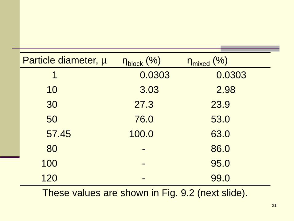
If the individual cyclone were one-half foot in diameter, the Wi in Eq. (10) would be about 0.125 ft (Note that Wi = 0.25Do from fig.9.4)

Repeating Example 5 for a Wi of 0.125 ft, we find a predicted cut diameter of 2.3 µ.

52

Next slide (Fig. 9.6) The comparisons of the predictions of Eqs. (8) and (9) and the following totally empirical data-fitting equation:

2

2

( / ) (11)1 ( / )

cut

cut

D DD D

η =+

54

The low collection efficiency, about 80%, of a typical cyclone shows that it cannot meet modern control standards (usually > 95% required control efficiency) for any particle group that has a substantial fraction smaller than 5 µ in diameter.

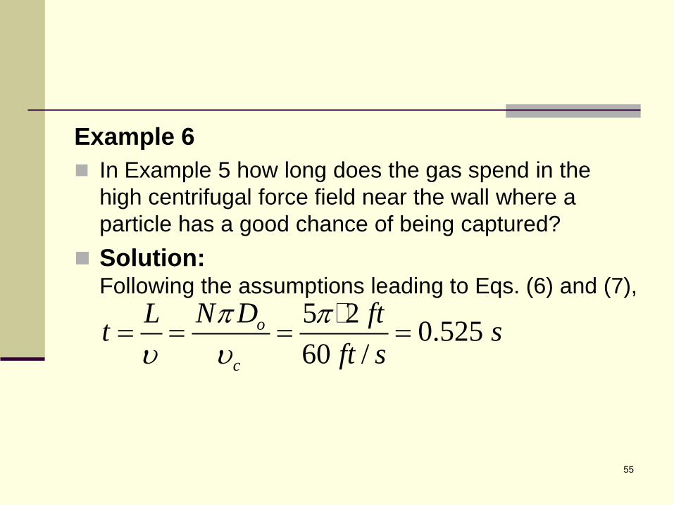
55

Example 6 In Example 5 how long does the gas spend in the

high centrifugal force field near the wall where a particle has a good chance of being captured?

Solution: Following the assumptions leading to Eqs. (6) and (7),

5 2 0.525 60 /

o

c

N DL ftt sft s

π πυ υ

= = = =

56

The distance the particle can move toward the wall is equal to the product of this time and vt, but vt is proportional to vc squared, so that to get better collection efficiency we must go to lower and lower times in the cyclone. (lower times means higher Vt and consequently higher Vc)

Previously we stated that the typical velocity at a cyclone inlet is 60 ft/s and that this velocity is selected for pressure drop reasons.

57

For a given cyclone one will generally find that the pressure drop, for various conditions, can be represented by an equation of the form: where ρg is the gas density and vi is the velocity at the inlet to the cyclone

(it is not the same as the velocity in the duct approaching the cyclone; typically it is about 1.5 times as high)

2

(12)2g i

in outP P P Kρ υ

∆ = − =

58

All sudden expansions have a K of 1.0, all sudden contraction have a K of 0.5, etc.

Most cyclone separators have Ks of about 8. It is common in air-conditioning design to

refer to the quantity (ρg v2 / 2) as a velocity head, so one could say that most cyclones have pressure drops of about 8 velocity heads.

59

Example 7 A cyclone has an inlet velocity of 60 ft/s and a

reported pressure loss of 8 velocity heads. What is the pressure loss in pressure units?

Solution: 2 2 2 2

2

22

18(0.075)(60 / ) ( / 32.2( ))( /144 . )2

0.23 / . 1,606 / 1.61 0.23 6.4 . #

P ft s lbf s lbm ft ft in

lbf inN m kPa psi in H O

∆ = ⋅ ⋅

=

= = = =

60

1.3 Electrostatic Precipitators (ESP)

The electrostatic precipitator is like a gravity settler or centrifugal separator, but electrostatic force drives the particles to the wall.

Centrifugal separators is not effective for particles below about 5 micron in diameter.

ESP is effective on much smaller particles than the previous two devices.

61

In all three kind of devices, the viscous (Stokes’ law) resistance of the particle to being driven to the wall is proportional to the particle diameter (Fd = 3πµDv).

For gravity and centrifugal separators, the force that can be exerted is proportional to the mass of the particle, which, for constant density, is proportional to the diameter cubed.

62

Thus the ratio of driving force to resisting force is proportional to (diameter cubed/diameter) or to D2.

As the diameter decreases, this ratio falls rapidly.

63

In ESPs the force moving the particle toward the wall is electrostatic.

This force is practically proportional to the particle diameter squared, and thus the ratio of driving force to resisting force is proportional to (diameter squared/diameter) or to D.

Therefore, the difficulty in ESPs is proportional to (1/D) rather than to (1/D2) as in gravitational or centrifugal devices.

64

The basic idea of all ESPs is to give the particles an electrostatic charge and then put them in an electrostatic field that drives them to a collecting wall.

This is an inherently two-step process. In one type of ESP, called a two-stage

precipitator, charging and collecting are carried out in separate parts of the ESP (used in building air conditioners and called electronic air filter).

65

For most industrial applications, the two separate steps are carried out simultaneously in the same part of the ESP.

The charging function is done much more quickly than the collecting function, and the size of the ESP is largely determined by the collecting function.

66

Next slide (Fig. 9.7) A wire-and-plate ESP with two plates.

68

The gas passes between the plates, which are electrically grounded (i.e., voltage = 0).

Between the plats are rows of wires, held at a voltage of typically -40,000 volts.

69

The power is obtained by transforming ordinary alternating current to a high voltage (-40,000 V) and then rectifying it to direct current through some kind of solid-state rectifier.

This combination of charged wires and grounded plates produces both the free electrons to charge the particles and the field to drive them against the plates.

70

On the plates the particles lose their charge and adhere to each other and the plate, forming a “cake”.

Solid cakes are removed by rapping the plates at regular time intervals with a mechanical or electromagnetic rapper that strikes a vertical or horizontal blow on the edge of the plate

Some of the cake is re-entrained, thereby lowering the efficiency of the system.

71

For liquid droplets the plate is often replaced by a circular pipe with the wire down its center.

Some ESPs (mostly the circular pipe variety) have a film of water flowing down the collecting surface, to carry the collected particles to the bottom without rapping.

72

There are many types of ESPs. Fig. 9.8 (next slide) shows one of the most

common in current use.

Main elements Perforated gas

distribution plate Discharge electrodes Collecting plates Rapping system Transformer-rectifier

sets

74

Each point in space has some electrical potential V.

If the electrical potential changes from place to place, then there is an electrical field, E = ∂V / ∂x, in that space. If we connect two such points with a conductor, then a current will flow.

The units of E are V/m. i.e. E is the gradient of V.

75

In a typical wire-and-plate precipitator, the distance from the wire to the plate is about 4 to 6 in., or 0.1 to 0.15 m.

With a voltage difference of 40 kV (since the plate is grounded) and 0.1 m spacing, one would assume a field strength of 40 kV/0.1 m = 400 kV/m.

This is indeed the field strength near the plate.

76

The driving potential near the wires must be much larger.

Typically it is 5 to 10 MV/m.

77

When a stray electron from any of a variety of sources encounters this strong a field, it is accelerated rapidly and attains a high velocity.

If it then collides with a gas molecule, it has enough energy to knock one or more electrons loose, thus ionizing the gas molecule.

78

These electrons are likewise accelerated by the field and knock more electrons loose, until there are enough free electrons to form a steady corona discharge.

The electrons migrate away from the wire, toward the plate.

79

As the electrons flow toward the plate, they encounter particles and can be captured by them, thus charging the particles and driving them to the plate.

80

Therefore, the roles of the electric field are: Creating the electrons Driving the electrons toward the plate Charging the particles (using the electrons)

and hence driving such charged particles toward the plate.

81

For particles larger than about 0.15 µ, the dominant charging mechanism is field charging.

As the particles become more highly charged, they bend the paths of the electrons away from them.

Thus the charge grows with time, reaching a steady state value of “q” (no more charging).

82

here q is the charge on the particle, and ε is the dielectric constant of the particle (a dimensionless number that is 1.0 for a vacuum, 1.0006 for air, and 4 to 8 for typical solid particles).

The permittivity of free space εo is a dimensionless constant whose value in the SI system of units is 8.85 x 10-12 C/(V • m).

D is the particle diameter, and Eo is the local field strength.

23 (13)2 o oq D Eεπ ε

ε = +

83

Example 8 A 1-µ diameter particle of a material with a dielectric

constant of 6 has reached its equilibrium charge in an ESP at a place where the field strength is 300 kV/m. How many electronic charges has it?

Solution: ( )( ) ( )212 6

1917

63 8.85 10 / / 10 300 /6 2

1.602 10 1.88 10 300 #

q C V m m kV m

electronsC electronsC

π − −

−

= × + ×

= × × =

84

85

The electrostatic force on a particle is Here Ep is the local electric field strength causing the force.

If we substitute for q from Eq. (13), we find The two subscripts on the Es remind us that one represents the field strength at the time of charging, the other the instantaneous (local) field strength.

pF qE=

23 (14)2 o o pF D E Eεπ ε

ε = +

86

For all practical purposes we use an average E; and in the rest of this chapter we will use Eo = Ep = E.

If the particle’s resistance to being driven to the wall by electrostatic forces is given by the Stokes drag force (Fd = 3πμDV) , we can set the resistance force equal to the electrostatic force in Eq. (14) and solve for the resulting velocity, finding:

2202

3 EDF εεεπ

+=

87

This velocity is called the drift velocity in the ESP literature, and is given the symbol ω (same as the terminal settling velocity, but with a different symbol)

( )22 (15)o

t

D E εεε

υ ωµ

+= =

88

Example 9 Calculate the drift velocity for the particle in Example

8. Solution:

6 12 5 2

5 2

(10 )(8.85 10 / / )(3 10 / ) (6 / 8) ( /( ))(1.8 10 / / )( /( ))

0.033 / 3.3 / 0.109 / #

m C V m V m N m C Vkg m s N s kg m

m s cm s ft s

ω− −

−

× × × ⋅ ⋅=

× ⋅ ⋅= = =

89

Eq. (15) shows that the drift velocity is proportional to the square of E, which is approximately equal to the wire voltage divided by the wire-to-plate distance.

If we could raise the voltage or lower the wire-to-plate distance, we should be able to achieve unlimited drift velocities.

The limitation here is sparking.

90

Occasionally an ionized conduction path will be formed between the wire and the plate; this ionized path is then a good conductor and forms a continuous standing spark (equivalent to a lightning stroke).

The power supply to the wire must sense this sudden increase in current and stop the flow into it to prevent a burnout of the transformer.

91

Normally the current is shut off for a fraction of a second, the lighting stroke ends, and then the field is reestablished.

As one raises the values of E, the frequency of sparks increases.

These sparks are energetic events that disrupt the cake on the plate, thus reducing the collection efficiency, so a large number of sparks are bad.

Aiming at zero sparks by lowering the voltage results in a low E and a lower efficiency

92

Most ESP control systems are set for about 50 to 100 sparks per minute.

Furthermore, it is common practice to subdivide the power supply of a large precipitator into many subsupplies so that each part of the precipitator can operate at the optimum voltage for its local conditions.

93

When we compare the drift velocity here with the terminal settling velocity computed for the same particle in a cyclone separator in Example 3, we see that this is only about five times as fast.

Why then is an ESP so much more effective than a cyclone for fine particle collection?

94

As mentioned before, the drift velocity is proportional to D for an ESP and to D2 for a cyclone

To obtain a high drift velocity in a cyclone, one must use a high gas velocity, thus, the residence time of the particle in a cyclone is very short.

95

On the other hand, the gas velocity does not enter Eq. (15), i.e. ω (or Vt) is independent of gas velocity. ►►we can make the precipitator large

enough that the particle spends a long time in it and has a high probability of capture.

Typical modern ESPs have gas velocity of 1 to 2 m/s, and the gas spends from 3 to 10 seconds in them (compare this to the 0.525 seconds obtained in the cyclone in example 6 and the high gas velocity required to get better efficiency in a cyclone) .

96

Recall from the gravity settlers:

avg

t

VHLV

=η

ESP equivalent (Fig. 9.7) Gravity (Fig. 9.1)

ω : The drift velocity Vt : terminal settling velocity

H : The distance from the wire to the plate.

H : the max distance perpendicular to the flow that a particle must travel

h L : collecting area (A) W L : collecting area

L : the max distance that a particle must travel within the device to be collected

L : the max distance that a particle must travel within the device to be collected

h H : the area perpendicular to the flow direction

W H : the area perpendicular to the flow direction

Vavg = Q / H h Vavg = Q / W H

97

Therefore, for ESP:

Eqn (16) is only theoretical and has no practical application.

Eq. (17) is the Deutsch-Anderson equation, the most widely used simple equation for design, analysis, and comparison of ESPs.

( ) QhL

HL

hHQ

ωωη ==

(16)blockA

Qωη =

1 exp (17)mixedA

Qωη

= − −

98

Example 10 Compute the efficiency-diameter relation for an ESP

that has particles with a dielectric constant of 6 and (A/Q) = 0.2 min/ft. we will use only the mixed flow equation.

Solution: Using the results of Example 9 we know that a 1-µ diameter particle will have a drift velocity of 0.109 ft/s, and that the drift velocity will be linearly proportional to the particle diameter.

99

Thus for a 1-µ particle we may compute

We can then make up a table using the drift velocity proportional to the particle diameter:

( )60 min1 exp (0.109 / )(0.2 min/ ) =0.73sft s ftη = − −

Particle diameter, µ η (%) 0.1 0.5 1 3 5

12.0 48.0 73.0 98.0 99.8

100

This example shows that this fairly typical precipitator has a cut diameter of about 0.5 µ, one-tenth of that of a typical cyclone.

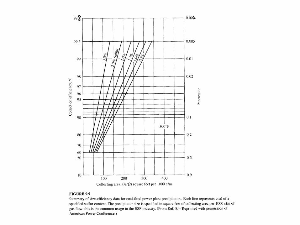
Eq. (17) suggests that if we pass a particle-laden gas stream through various precipitators, all of the data for this stream will form a straight line on a plot of log p vs. A/Q, where p = 1-η.

Fig. 9.9 (next slide) is such a plot.

102

Example 11 From Fig. 9.9, estimate the value of ω for coal

containing 1% sulfur. Solution:

From the figure at 99.5% efficiency we read that for 1% sulfur coal,

From Eq. (17)

2

3

310 0.311000 /

A ft minQ ft min ft= =

ln ln 0.0051 17.09 0.28 8.6 #/ 0.31 / minp ft ft cm

A Q min ft s sω = = − = = =

103

The different lines for different coal sulfur contents on Fig. 9.9 are caused by sulfur’s indirect effect on fly ash resistivity (discussed later).

ESPs work well with medium-resistivity solids, but poorly with low-resistivity or high-resistivity solids.

We can see why by referring to Fig. 9.10 (next slide).

105

For the case of a low-resistivity solid, e.g., carbon black, the material forms a cake that is a good conductor of electricity.

The voltage gradient in the cake is small. On reaching the plate the particles are

discharged and hence there is very little electrostatic force holding the collected particles to the plate.

The collected particles do not adhere and are easily re-entrained; the overall collection is poor.

i.e. particles are easily charged (very conductive) and rapidly lose their charge on arrival at the collection electrode

106

Fig. 9.10 also shows particles of very high resistivity on the plate.

Here most of the voltage gradient occurs through the cake, causing at least two problems.

First, the voltage gradient near the wire has now fallen so much that it cannot produce a good corona discharge. (particles are not easily charged)

107

Second, the voltage gradient inside the cake is so high that in the gas spaces between the particles stray electrons will be accelerated to high velocities and will knock electrons off of gas molecules and form a back corona inside the cake.

This back corona is a violently energetic conversion of electrostatic energy to thermal energy that causes minor gas explosions, which blow the cake off the plate and make it impossible to collect the particles.

108

The practical resistivity range is greater than 107 and less than 2 x 1010 ohm · cm.

If the resistivity of the particles is too low, little can be done.

If the resistivity is too high, there are some possibilities.

109

The resistivity of many coal ashes is too high at 300oF for good collection, but satisfactorily low at 600oF. Therefore, adjusting the temperature is one solution

If one could condense on its surface a conducting material, the ash resistivity would be reduced.

Some of the sulfur in coal is converted in the furnace to SO3, which collects on the ash, absorbs water, and makes the ash more conductive.

110

Therefore, one logical cure is to add SO3 to the gas stream to “condition” the ash.

Since coal ash is basic, an acidic conditioner seems best.

For acidic streams such as Portland cement, a basic conditioner such as ammonia works best.

.

111

112

113

Another approach to the ash resistivity problem is to separate the charging and collecting functions. If the particles are charged in a separate

charger, one can use a higher voltage and not worry much about the resulting sparks, because they do not pass through the cake and disrupt it.

114

Table 9.2 (next slide) shows some representative values of ω (effective drift velocity) for industrial precipitators.

116

Example 12 Our ESP has a measured efficiency of 90%.

We wish to upgrade it to 99%. By how much must we increase the collecting area?

Solution: Using Eq. (17): 1 0.1 exp

1 0.01 exp

existingexisting existing

newnew new

Ap

Q

ApQ

ωη

ωη

− = − = =

−

= − = =

117

Unfortunately life is harder than that. In Eq. (15) we found that the drift velocity is proportional to the particle diameter.

Thus, as the percentage efficiency by weight increases, the remaining particles become smaller and smaller and harder and harder to collect.

/ln 0.1 0.5ln 0.01 /

thus, 2 #

existing existing

new new

new

existing

A Q AA Q A

AA

ωω

−= = =

−

=

118

To take this phenomenon into account, some designers use a modified Deutsch-Anderson equation with the form: Where k is an arbitrary exponent, typically about 0.5.

1 exp ( / ) (18)kp A Qη ω = − = −

119

Example 13 Rework Example 12 using Eq. (18) instead of Eq.

(17), taking k = 0.5. Solution:

Here for the existing unit (ωA/Q) = (-ln p)1/k = (-ln 0.1)2 = 5.30. For the upgraded precipitator we need (ωA/Q) = (-ln 0.01)2 = 21.20.

So the new value of (A/Q)-assuming constant ω-is (21.20/5.30) = 4.0 times the old value of (A/Q). #

120

Example 14 A precipitator consists of two identical

sections in parallel, each handling one-half of the gas. It is currently operating at 95% efficiency. We now hold the total gas flow constant, but maldistribute the flow so that two-third of the gas goes through one of the sections, and one-third through the other. What is the predicted overall collection efficiency?

121

Solution: For the existing situation (using Eq. (17)) For the new situation:

0.05 exp

ln 0.05 2.995

ApQ

AQ

ω

ω

= = −

= − =

1

2

1/ 2exp( 2.995) 0.10572 / 31/ 2exp( 2.995) 0.01111/ 3

p

p

= − = = − =

122

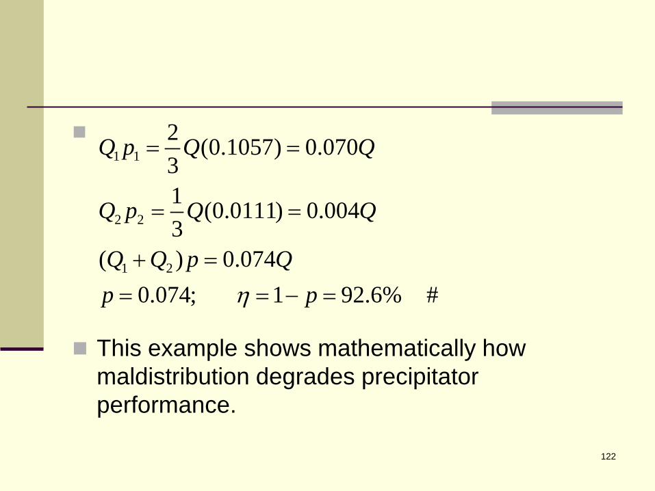
This example shows mathematically how maldistribution degrades precipitator performance.

1 1

2 2

1 2

2 (0.1057) 0.07031 (0.0111) 0.0043

( ) 0.0740.074; 1 92.6% #

Q p Q Q

Q p Q Q

Q Q p Qp pη

= =

= =

+ == = − =

123

The typical pressure drop of a ESP is 0.1 to 0.5 in. H2O, much lower than that in a cyclone.

The pressure drop in the ducts leading to and from the precipitator is generally more than in the ESP itself.

The collection requirements of ESPs have been pushed from the 90~95% range typical in 1965 to the 99.5%-plus range now commonly specified.

124

The ESP industry is now well established. Standard package units are available for small flows (down to the size of home air conditioners), and large power plants have precipitators costing up to $30 million.

125

2. Dividing Collection Devices

Filters and scrubbers do not drive the particles to a wall, but rather divide the flow into smaller parts where they can collect the particles. A filter can be either a surface filter or a depth filter.

2.1 Surface Filters A surface filter is a membrane (sheet steel,

cloth, wire mesh, or filter paper) with holes smaller than the dimensions of the particles to be retained.

126

However, one only needs to ponder the mechanical problem of drilling holes of 0.1-µ diameter or of weaving a fabric with threads separated by 0.1µ to see that such filters are not easy to produce.

They are much too expensive and fragile for use as high-volume industrial air cleaners.

They have analytical uses for determining the chemical identity and size distribution of air pollution particles.

127

Although industrial air filters rarely have holes smaller than the smallest particles captured, they often act as if they did.

The reason is that, as fine particles are caught on the sides of the holes of a filter, they tend to bridge over the holes and make them smaller.

Thus as the amount of collected particles increases, the cake of collected material becomes the filter.

128

The particles collect on the front surface of the growing cake.

For that reason this is called a surface filter. The flow through a simple filter is shown

schematically in Fig. 9.12.

130

The frictional resistance to flow through the filter cake and the filter medium will cause a decrease in pressure.

131

In most industrial filters, both for gases and liquids, the flow velocity in the individual pores is so low that the flow is laminar.

Therefore, we may use the well-known relations for laminar flow of a fluid in a porous medium, which indicate Here, k is the permeability, a property of the bed.

(19)sQ p kA x

υµ

−∆ = = ∆

132

For a steady fluid flow through a filter cake supported by a filter medium, there are two resistances to flow in series, but the flow rate is the same through each of them.

We find:

Solving for P2, we get

2 31 2

cake filter

-P=sPP P k k

x xυ

µ µ − = ∆ ∆

2 1 3cake filter

=s sx xP P P

k kµυ µυ∆ ∆ = − +

133

Then solving for vs:

This equation describes the instantaneous flow rate through a filter; it is analogous to Ohm’s law for two resistors in series.

The Δx/k terms are called the cake resistance and the cloth resistance.

1 3( ) (20)[( / ) ( / ) ]s

cake filter filter

p p Qvx k x k Aµ

−= =

∆ + ∆

134

The resistance of the filter medium is usually assumed to be a constant that is independent of time, so (Δx/k)filter is replaced with a constant α.

If the filter cake is uniform, then its resistance is proportional to its thickness:

1

1

cakecake

cake

mass of cakexarea

volume of gas mass of solids removedarea volume of gas

ρ

ρ

∆ = =

135

Customarily we define: Here W is the volume of cake per volume of gas processed, which corresponds to a collection efficiency, η, of 1.0.

For most surface filters η=1.0, so the η is normally dropped. Thus Here V is the volume of gas cleaned.

1 cake

mass of solids removed volume of cakeWvolume of gas volume of gas processed

ηρ

= =

( ) and (21)cakecake s

d xVx W WA dt

υ∆ ∆ = =

136

Substituting Eq. (21) for the cake thickness in Eq. (20), we find

For most industrial gas filtrations the filter is supplied by a centrifugal blower at practically constant pressure, so (P1-P3) is a constant, and Eq. (22) may be rearranged and integrated to

1 3(P -P )Q 1 dV= = = (22)A A dt [(V /kA+ ]s W

υµ α

2

1 3( ) (23)2

V W V P P tA k A

µ µα + = −

137

For many filtrations the resistance α of the filter medium is negligible compared with the cake resistance, so the second term of Eq. (23) may be dropped.

The two most widely used designs of industrial surface filters are shown in Figs. 9.13 and 9.14 (next and second slides).

J

140

For the baghouse in Fig. 9.13 (shake-deflate design) there must be some way of removing the cake of particles that accumulates on the filters.

Normally this is not done during gas-cleaning operations.

A weak flow of gas in the reverse direction may also be added to help dislodge the cake, thus deflating the bags.

Often metal rings are sewn into filter bags at regular intervals so that they will only partly collapse when the flow in reversed.

141

Because it cannot filter gas while it is being cleaned, a shake-deflate baghouse cannot serve as the sole pollution control device for a source that produces a continuous flow of dirty gas.

Typically, for a major continuous source like a power plant, about five baghouses will be used in parallel, with four operating as gas cleaners during the time that the other one is being shaken and cleaned.

Each baghouse might operate for two hours and then be cleaned for 10 minutes.

142

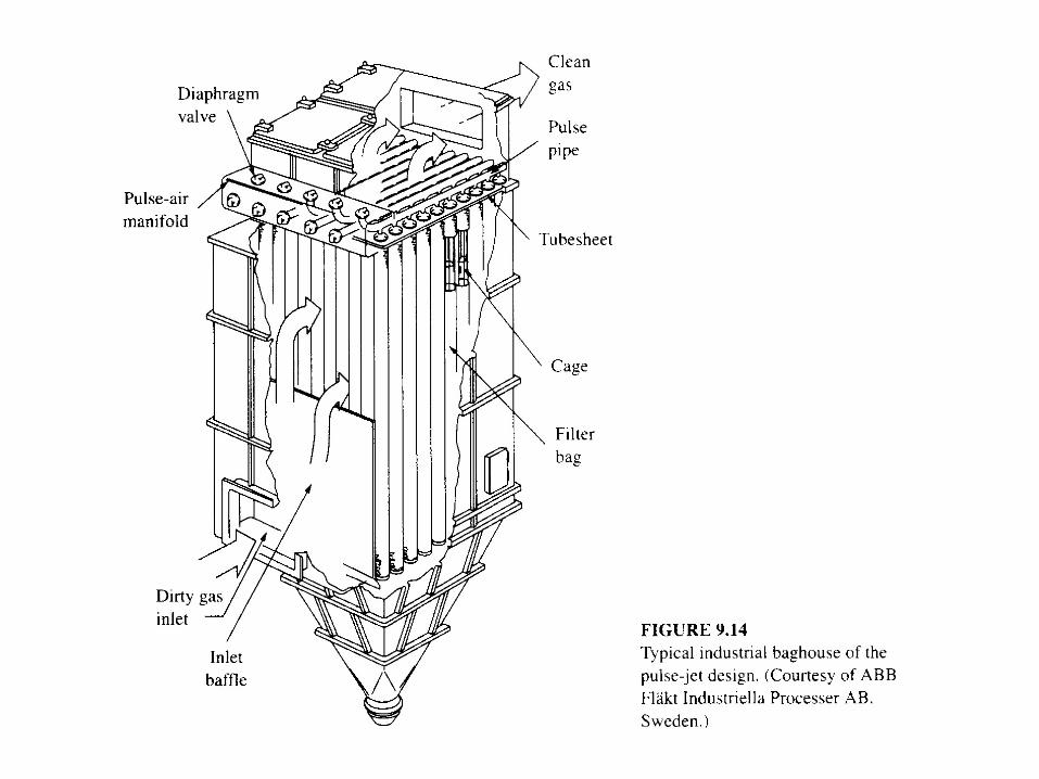
The other widely used baghouse design, called a pulse-jet filter, is shown in Fig. 9.14.

In it the flow during filtration is inward through the bags, which are similar to the bags in Fig. 9.13 except their ends open at the top.

The bags are supported by internal wire cages to prevent their collapse.

143

The bags are cleaned by intermittent jets of compressed air that flow into the inside of the bag to blow the cake off.

Often these baghouses are cleaned while they are in service.

144

Example 15 The shake-deflate baghouse on a power

station has six compartments, each with 112 bags that are 8 in. in diameter and 22 ft long, for an active area of 46 ft2 per bag.

The gas being cleaned has a flow rate of 86,240 ft3/min.

The pressure drop through a freshly cleaned baghouse is estimated to be 0.5 in. H2O.

145

The bags are operated until the pressure drop is 3 in. H2O, at which time they are taken out of service and cleaned.

The cleaning frequency is once per hour. The incoming gas has a particle loading of 13

grains/ft3.

146

The collection efficiency is 99%, and the filter cake is estimated to be 50% solids, with the balance being voids.

Estimate how thick the cake is when the bags are taken out of service for cleaning. What is the permeability, k, of the cake?

147

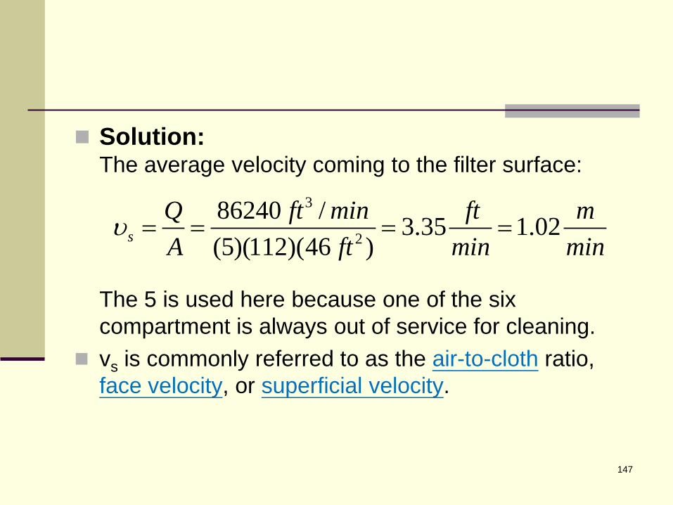
Solution: The average velocity coming to the filter surface: The 5 is used here because one of the six compartment is always out of service for cleaning.

vs is commonly referred to as the air-to-cloth ratio, face velocity, or superficial velocity.

3

2

86240 / 3.35 1.02(5)(112)(46 )s

Q ft min ft mA ft min min

υ = = = =

148

If the filter remains in service for 1 hour before cleaning and vs is constant, the 1 square foot of bag will collect the following mass of particles:

( )3

2 2

60 13 3.35 0.99 (1 )7000

0.369 1.80

sm gr lbm ft minc t hA ft gr min h

lbm kgft m

υ η = =

= =

149

The thickness of the cake collected in 1 hour is

Taking

2

3 3 3

3

/ 0.369 /(2 / )(0.5)(62.4 / / )

5.9 10 0.071 . 1.8

m A lbm ftg cm lbm cm ft g

ft in mmρ

−

=⋅

= × = =

0, we can solve Eq. (20) for k, filter

xk

α∆ = =

5 2

22 2

12 2 13 2

(3.35 / min)(0.071 /12 .)(0.018 )(2.09 10 / / )( / 60 )( ) (3 . )(5.202 / / . )

7.96 10 7.40 10

s x ft ft in cp lbf s ft cp min skp in H O lbf ft in H O

ft m

υ µ −

− −

∆ × ⋅= =

−∆

= × = ×

150

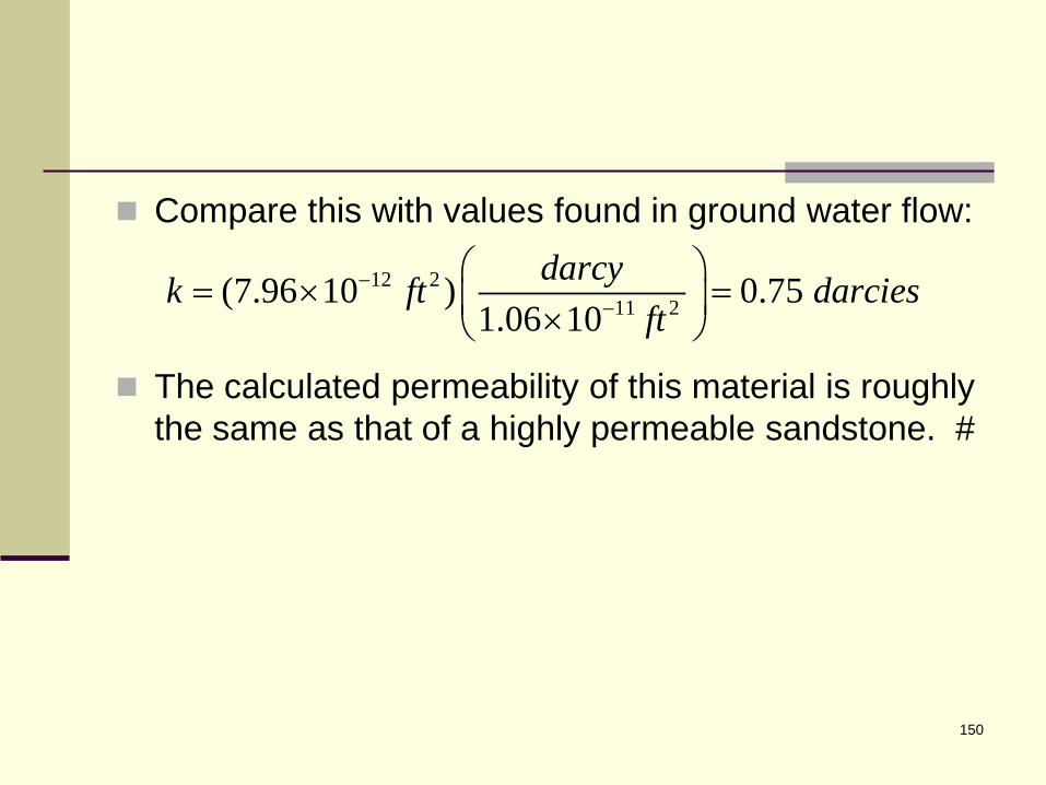
Compare this with values found in ground water flow:

The calculated permeability of this material is roughly the same as that of a highly permeable sandstone. #

12 211 2(7.96 10 ) 0.75

1.06 10darcyk ft darcies

ft−

−

= × = ×

151

This calculation shows that the collected is about 1.8 mm thick.

If the cleaning were perfect, this would be the cake thickness.

However, it is hard to clean the bags completely, and in power plant operation it is common for the average cake thickness on the bags to be up to 10 times this amount.

152

One of the advantages of the pulse-jet design is that it cleans the bags more thoroughly, allowing a higher vs, at the cost of a somewhat shortened bag life.

Fig. 9.15 (next slide) is a set of typical results from tests of collection efficiency for this kind of filter.

154

Consider the lower curve in Fig. 9.15 for which the superficial velocity is 0.39 m/min.

At zero fabric loading (newly or freshly cleaned cloth) the outlet concentration is high and practically equal to the inlet concentration (0.8 g/m3).

As the cake builds up, the outlet concentration declines, finally stabilizing at a value about 0.001 times the inlet concentration (i.e. η = 99.9 percent)

155

Once the cake has been properly established, the filtration efficiency remains constant.

But why do any particles at all get through?

156

If the superficial velocity increases, the efficiency falls; for a superficial velocity of 3.35 m/min the outlet concentration is about 20 percent of the inlet concentration.

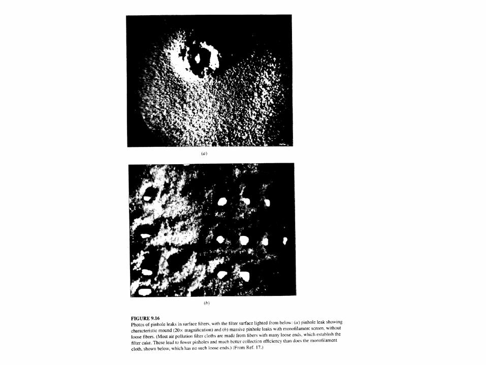
The particles that pass through such a filter do not pass through the cake but through pinholes, which are regions where the cake did not establish properly (Fig. 9.16, next slide).

158

The pinholes are apparently about 100 µ in diameter, much too large for a single particle to block because there are rarely 100-µ particles in the streams being treated.

When the superficial velocity is high, more pinholes form, and thus a higher fraction of the flow passes through the pinholes than when it is low.

159

Example 16 Estimate the velocity through a pinhole in a filter

with a pressure drop of 3 in. of water. Assuming that this is the pressure drop

corresponding to the curve for 0.39 m/min on Fig. 9.15, that the steady-state penetration at that velocity is 0.001, and that the pinholes have a diameter of 100 µ, estimate how many pinholes per unit area there are in the cake.

160

Solution: The flow through the pinhole is best described by Bernoulli’s equation, from which we find the average velocity:

Here the (area ∙velocity) of the pinholes must be 0.001 times the (area ∙velocity) of the rest of the cake. Hence

1/ 21/ 22

3 22

2 2(3 ) 249 0.61(1.20 / )

21.5 /

pinholesP in H O Pa kgC

kg m in H O Pa m s

m s

υρ

∆ ⋅ = = ⋅ ⋅ ⋅ =

27

2

0.001 0.001 (0.39 / ) 3.0 10(21.5 / )(60 / )

pinholes s

cake pinholes

A m min mA m s s min m

υυ

−= = = ×

161

Each pinhole has an area of A = (100 10-6 m)2 (π/4) = 7.85 10-9 m2, so there must be

The calculated velocity through a pinhole is (21.6 x 60) /0.39 = 3300 times the velocity through the cake.

72

9 2

3.0 10 38 pinholes/m #7.85 10 m

−

−

×=

×

162

If surface or cake-forming filters are operated at low superficial velocities, they can have very high efficiencies, and they generally collect fine particles as efficiently as coarse ones.

Therefore, surface filters have found increasing application, particularly in electric power plants, where regulations are becoming more stringent requiring the collection of particles in the size range from 0.1 to 0.5 microns, which are difficult for ESPs to collect.

163

2.2 Depth Filter

Filters do not form a coherent cake on the surface, but instead collect particles throughout the entire filter body are called depth filters.

An example with which the student is probably familiar is the filter on filter-tipped cigarettes.

164

In both of these a mass of randomly oriented fibers (not woven to form a single surface) collects particles as the gas passes through it.

165

2.3 Filter Media

For shake-deflate baghouses, the filter bags are made of tightly woven fibers (surface filter), much like those in a pair of jeans.

Pulse-jet baghouses use high strength felted fabrics, so that they act partly as depth filters and partly as surface filters. This allows them to operate at superficial

velocities (air-to-cloth ratios) two to four times those of shake-deflate baghouses.

This higher capacity per unit size has allowed them to take market share away from the previously dominant shake-deflate type baghouse.

166

Filter Fabrics are made of cotton, wool, glass fibers, and a variety of synthetic fibers.

Cotton and wool cannot be used above 180 and 200oF, respectively, without rapid deterioration, whereas glass can be used to 500oF (and short-time excursions to 550oF).

167

In addition the fibers must be resistant to acids or alkalis if these are present in the gas stream or the particles as well as to flexing wear caused by the repeated cleaning.

Typical bag service life is 3 to 5 years.

168

Fabric Selection Chart

169

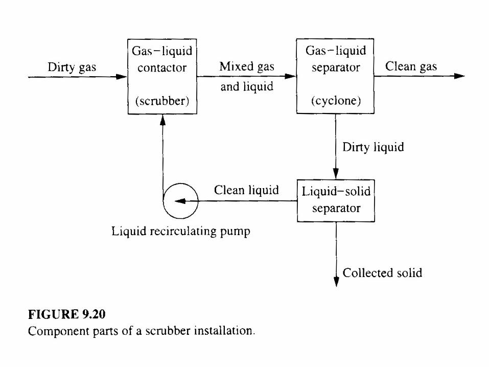
2.4 Scrubbers for Particulate Control Scrubbers effectively divide the flow of

particle-laden gas by sending many small drops through it.

Most fine particles will adhere to a liquid drop if they contact it.

170

Particles 50 µ and larger are easily collected in cyclones.

If our problem is to collect a set of 0.5 µ particles, cyclones will not work at all.

However, if we were to introduce a large number of 50 µ diameter drops of a liquid (normally water) into the gas stream to collect the fine particles, then we would pass the stream through a cheap, simple cyclone and collect the drops and the fine particles stuck on them.

171

A complete scrubber has several parts, as sketched in Fig. 9.20 (next slide).

173

2.4.1 Collection of Particles in a Rainstorm

Fig. 9.21 (next slide) shows the geometry for which we will make a material balance on the particles and on the drops.

175

We consider a space with dimensions Δx, Δy, Δz.

The concentration of particles in the gas in this space in c.

Now we let one spherical drop of water of diameter DD pass through this space.

How much of the particulate matter in the space will be transferred to the drop?

176

We can see that the volume of space swept out by the drop is the cylindrical hole shown in Fig. 9.21, whose volume is

The total mass of particles that was originally in that swept volume is that volume times the concentration c.

2 4swept by one drop DV D zπ

= ∆

177

The fraction of these that will be collected by the drop is the target efficiency ηt, which we can determine from Fig. 9.18 or its equivalent.

So the mass of particles transferred from the gas to the drop is

( )

2D t

mass transferred swept target= concentration

to one drop volume efficiencyπ = DΔzcη4

178

Next we consider a region of space (still ΔxΔy Δz) that is large with respect to the size of any one individual raindrop through which a large number of raindrops are falling at a steady rate ND, expressed as drops/time.

From a material balance on the particles in the space, we can say that

22

( )( o / )-( )

( / 4)( ) - - (27)4

D t D DD t

dc mass transferred to each drop number f drops timedt volume of the region

D zc N ND cx y z x y

π η π η

=

∆= = ∆ ∆ ∆ ∆ ∆

179

We multiply top and bottom of Eq. (27) by the volume of a single spherical drop and simplify to:

The final term in parentheses in Eq. (28) represents the volume of rain that fell per unit time divided by the horizontal area through which they fell (rainfall rate).

3( / 6)1.5 (28)t D D

D

cdc N Ddt D x y

η π = − ∆ ∆

180

For the rest of this chapter the total liquid volumetric flow rate going to a scrubber will have the symbol QL, so the rightmost term is QL/A, where A is the horizontal projection of the region of interest.

Substituting this into Eq. (28), we can rearrange and integrate to find

1.5

1.5 (29)

Lt

D

Lt

o D

dc Qcdt D A

c Qlnp ln tc D A

η

η

= −

= = − ∆

181

Example 21 A rainstorm is depositing 0.1 in./h, all in the

form of spherical drops 1 mm in diameter. The air through which the drops are falling

contains 3 µ diameter particles at an initial concentration 100 µg/m3.

What will the concentration be after one hour?

182

Solution: Solving Eq. (29) for c, we find

From Fig. 8.7 we can read the terminal settling velocity of a 1-mm diameter drop of water in still air is about 14 ft/s = 4.2 m/s, so we can compute Ns from Eq. (25) as

Note: Ns is called the separation number. It is mentioned in the depth filter section. It is equal to the Stokes stopping distance divided by the diameter of the barrier

1.5 t Lo

D

Q tc c expD Aη ∆

= −

2 3 6 2

5 3

(2000 / )(3 10 ) (4.2 / ) 0.2318 (18)(1.8 10 / / )(10 )

PS

D

D kg m m m sND kg m s m

ρ υµ

−

− −

×= = =

×

183

From Fig. 9.18 we can read ηt ≈ 0.23, so

This example shows that the result depends on the total amount of rain that fell, QL Δt/A, which is 0.1 inch in this case, not on the time or rainfall rate separately.

#3 3 3

(1.5 0.23)(0.1 . / )(1 )100 43 10 39.37 .

g in h h m gc expm m in mµ µ

−

× = − =

184

If the example had asked for the collection efficiency for particles of 1 µ diameter, we would have calculated an NS one-ninth as large, and from Fig. 9.18 we would have computed an ηt of zero.

This calculation suggests that a rainstorm does not clean the air well.

185

2.4.2 Collection of Particles in Crossflow, Counterflow, and Co-flow Scrubbers

(1) Crossflow Scrubbers Fig. 9.22 (next slide)

Schematic of a crossflow scrubber.

187

A parcel of air moving through this scrubber behaves just like a parcel of air standing still in a rainstorm.

The linear velocity of the gas is (QG/ΔyΔz), and hence the time it takes a parcel of gas to pass through is the length of the scrubber divided by the linear velocity, or

(30)G

x y zTravel time tQ

∆ ∆ ∆= ∆ =

188

Substituting Eq. (30) into Eq. (29), we find

This equation says that the smaller the drop and the taller the scrubber, the more efficient it will be in removing particles.

1.5 (31)t L

o D G

c Qln p ln zc D Q

η= = − ∆

189

However, a small drop has a much lower vertical velocity, so it will be carried along in the flow direction by the gas and not be collected in the scrubber.

For this reason, this type of scrubber is not widely used.

190

(2) Counterflow Scrubber Next slide (Fig. 9.23)

Schematic of a counterflow scrubber

192

(3) Co-flow Scrubbers Clearly we need a geometrical arrangement

in which we can get very small drops to move at high velocities relative to the gas being scrubbed, to get a high Ns and high ηt, without blowing the drops out the side or top of the scrubber.

the solution to this problem is the Co-flow scrubber, shown schematically in Fig. 9.24 (next slide).

194

The liquid enters at right angles to the gas flow. Very high gas velocities can be used in this type

of scrubber, as much as 400 ft/s (122 m/s). The liquid enters with zero or negligible velocity

in the x direction so that at the inlet the relative velocity may be as high as 400 ft/s.

This may be 100 times the maximum tolerable relative velocity in a crossflow or counterflow scrubber.

196

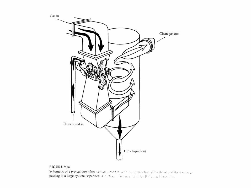
For the venturi shown in Fig. 9.26 the throat cross-sectional area is about one-fifth that at the inlet or outlet, so the velocity there must be about five times the velocity at the inlet or outlet.

To achieve high velocities in a gas flow we must have a drop in pressure (the larger the pressure drop, the larger velocities we obtain)

197

A venturi co-flow scrubber seems the most economical way to get a high velocity for rapid liquid breakup into drops and high collection efficiency with minimum fan power.

198

2.4.3 Pressure Drop in Scrubbers

Venturi scrubbers have higher pressure drops and higher efficiencies than the crossflow and counterflow scrubbers.

The power cost of the fan that drives the contaminated gas through a venturi scrubber often is much more important than the purchase cost of the scrubber.

199

Example 24 A typical venturi scrubber has a throat area of

0.5 m2, a throat velocity of 100 m/s, and a pressure drop of 100 cm of water = 9806 N/m2.

If we have a 100% efficiency motor and blower, what is the power required to force the gas through this venturi?

200

Solution:

If the fan and scrubber operate 8760 h/yr and the electricity costs 5 cents/kWh, the annual power cost will be Power cost = (245 kW)(8760 h/yr) ($0.05/kWh) = $ 107,300/yr #

( )22 3

100 0.5 980610

245 328

Gm N kW sPower Q p m

s m N mkW hp

= ∆ =

= =

201

The pressure drop in a scrubber can be calculated by:

G

LLG Q

Qpp ρυ 221 =−

202

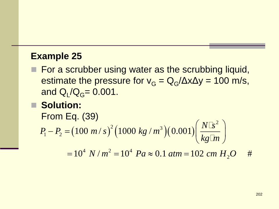
Example 25 For a scrubber using water as the scrubbing liquid,

estimate the pressure for vG = QG/ΔxΔy = 100 m/s, and QL/QG= 0.001.

Solution: From Eq. (39) ( ) ( )( )

22 3

1 2

4 2 42

100 / 1000 / 0.001

10 / 10 0.1 102 #

N sP P m s kg mkg m

N m Pa atm cm H O

− =

= = ≈ =

203

Unfortunately, the very properties that cause wet scrubbers to have high pressure drops are the same ones that make them efficient particle collectors: the rapid acceleration of liquid by the fast-moving gas produces both effects.