Control of discrete time systems based on recurrent Super ...verona.fi-p.unam.mx/~lfridman/publicaciones/papers/ISA.pdfiva.pdf · Control of discrete time systems based on recurrent

ISA Transactions ∎ (∎∎∎∎) ∎∎∎–∎∎∎

Contents lists available at ScienceDirect

ISA Transactions

http://d0019-05

n CorrE-m

PleasTran

journal homepage: www.elsevier.com/locate/isatrans

Control of discrete time systems based on recurrentSuper-Twisting-like algorithm

I. Salgado a, S. Kamal e, B. Bandyopadhyay b, I. Chairez c,n, L. Fridman d

a Centro de Innovación y Desarrollo Tecnológico en Cómputo (CIDETEC), Instituto Politécnico Nacional, Mexico City, Mexicob SYSCON, Indian Institute of Technology, Bombay, Mumbai, Indiac Departamento de Bioprocesos, Unidad Profesional Interdisciplinaria de Biotecnología (UPIBI), Instituto Politécnico Nacional, Av. Acueducto de Guadalupes/n col. Barrio la Laguna, Gustavo A. Madero, Mexico City, DF, Mexicod Engineering Universidad Nacional Autónoma de México, Mexico City, Mexicoe Department of Systems Innovation and Informatics, Kyushu Institute of Technology, Kitakyushu, Japan

a r t i c l e i n f o

Article history:Received 14 September 2015Received in revised form8 February 2016Accepted 23 April 2016

been less developed. In this paper, a discrete time super-twisting-like algorithm (DSTA) was proposed tosolve the problems of control and state estimation. The stability proof was developed in terms of the

This paper was recommended for publica-tion by Oscar Camacho

Keywords:Sliding mode controlDiscrete-time super twisting algorithmSliding mode differentiatorElectro-mechanical systems

x.doi.org/10.1016/j.isatra.2016.04.02478/& 2016 ISA. Published by Elsevier Ltd. All

esponding author.ail address: [email protected] (I. Chairez).

e cite this article as: Salgado I, et asactions (2016), http://dx.doi.org/10.1

a b s t r a c t

Most of the research in sliding mode theory has been carried out to in continuous time to solve theestimation and control problems. However, in discrete time, the results in high order sliding modes have

discrete time Lyapunov approach and the linear matrix inequalities theory. The system states trajectorieswere ultimately bounded inside a small region dependent on the sampling period. Simulation resultstested the DSTA. The DSTA was applied as a controller in a Furuta pendulum and as a signal differentiatorand as a controller in close loop for a DC motor.

& 2016 ISA. Published by Elsevier Ltd. All rights reserved.

1. Introduction

Advanced control techniques such as Sliding Modes (SM) allowthe control of uncertain nonlinear systems when they are affectedby modeling imprecisions or external perturbations. Classicalfeatures exhibited by sliding modes are robustness with respect toexternal matched uncertainties and finite time convergence. A SMscheme is obtained by inducing a discontinuity in the controlstructure. The discontinuous injection must be designed such thatthe trajectories of the system are forced to remain on some surfacedefined in the state space. The resulting motion on that surface isreferred as sliding mode [1]. In continuous time systems, the SMhave been extensively studied, the main theoretical results arepresented in [1,2], and references therein. In continuous time, thesecond order sliding mode solutions (SOSM) preserve the maincharacteristics of classical SM while reduce the undesirable chat-tering effect [3,4].

On the other hand, SM in discrete-time or discrete slidingmodes (DSM) generate the so-called quasi-sliding regime (QSM)and it has been less developed than the continuous case. The firstideas in DSM were introduced by [5,6] where a QSM is established

rights reserved.

l. Control of discrete time016/j.isatra.2016.04.024i

for systems with relative degree one. In [7], the study of SISOnonlinear systems with relative degree more than one is treated. Anew definition of a QSM regime is addressed in [8], where themotion of the system is restricted inside a certain band around thesliding hyperplane. In [9,10], some new developments on QSMhave been reported for several classes of discrete-time linearsystems. An approach to control discrete time systems using thefast output technique is considered when the system states are notneeded on-line [11]. The idea of second order sliding mode controlin discrete time systems has been introduced in terms of certainclass of discretizations [12]. Although in [13,14] a sort of dis-cretization has been applied on high order sliding mode con-trollers, the results are not reported in the literature so far, whichdeals with the concept of high-order discrete time sliding modecontrol (HDSM).

In this study, a new strategy to develop a Lyapunov like func-tion for the so-called discrete time Super-Twisting-like Algorithm(DSTA) is proposed. This name is used considering the similaritiesbetween the Euler discretization applied on the continuous ver-sion of the super-twisting method. In this scheme, the systemtrajectories are confined into a boundary layer in the vicinity of thesliding surface and stays inside it forever. The upper bound for thetracking error applying the DSTA is depending on the samplingperiod to the square power. The stability analysis is made in terms

systems based on recurrent Super-Twisting-like algorithm. ISA

www.sciencedirect.com/science/journal/00190578

www.elsevier.com/locate/isatrans

http://dx.doi.org/10.1016/j.isatra.2016.04.024



mailto:[email protected]





I. Salgado et al. / ISA Transactions ∎ (∎∎∎∎) ∎∎∎–∎∎∎2

of the discrete-time Lyapunov theory. Sufficient conditions for theexistence of QSM by means of a LMI are proposed.

In Section 2, the concept of high-order sliding modes (HOSM) isintroduced. Some mathematical background on the stability of discretetime nonlinear systems is given in Section 3. Then, a discrete timesuper-twisting control, a particular type of discrete time second ordersliding mode control is presented in Section 4. The result about theconvergence of the proposed algorithm is established in terms of asimple quadratic Lyapunov function. In Section 5, numerical examplesare presented. The first example is regarding the stabilization problemof a Furuta Pendulum. Then, the DSTA is tested as a robust signal dif-ferentiator following the result given in [15]. In close loop, the trajectorytracking problem for a DC motor is presented as a second example.Finally in Section 6 some conclusions are established.

2. Concept of high-order sliding modes

First, let us briefly introduce the high-order SM controllersconcept applied on continuous time systems. Consider a smoothdynamic system _x ¼ f xð Þþg xð Þu, where xARn is the system state,uAR is the scalar control, f : Rn-Rn and g xð Þ : Rn-Rn are somesmooth functions. High-order sliding manifold is given as follows.Consider that the set

sr ¼ x :dk

dtkσ xð Þ ¼ 0; k¼ 0;1;…; r�1

( ); ð1Þ

is non-empty and consists locally of Filippov trajectories, where σis a smooth function (this is considered as the sliding variable).The trajectories of these functions provide the successive timederivative of σ. The motion on set (1) is called rth-order slidingmode [18], which gives the dynamic smoothness degree in somevicinity of the sliding mode.

The relative degree r of the system is assumed to be constantand known. In other words, the first time at control explicitlyappears in the rth total time derivative of σ is σr ¼ h t; xð Þþ l t; xð Þu,where

h t; xð Þ ¼ σr j u ¼ 0;

l t; xð Þ ¼ ∂∂u

σra0; 0okmr ∂∂u

σrrkM ;

σr��

u ¼ 0rc; km; kM ; cARþ :

For finite time stabilization at origin, u takes the form given byu¼φ σ; _σ ;…;σrð Þ. Based on this concept, several sliding mode con-trollers (the sub-optimal controller [16], twisting controller [17], theterminal sliding mode controller [18] and super twisting controller [19])were proposed in continuous time. Moreover, a general output basedcontroller for rth relative degree system has been also developed.

Formulating HDSM, Wang et al., firstly discretized the continuoustime SMC and after that equivalent control based SMC system withthe relative degree higher than one is formulated in the canonicalform for designing the controller [13]. To define the sliding set, theyreplaced high order derivatives of the sliding mode by their respectivediscrete counterpart such as _σ ð�Þ≔σ kþ1ð Þ. Using invertible statetransformation matrix, they conclude that the original state isasymptotically stable.

3. Mathematical background

The following result is needed to demonstrate the convergenceresults for the DSTA.

Theorem 1. [20] Consider the nonlinear dynamic system

x1 kþ1ð Þ ¼ f 1 x1 kð Þ; x2 kð Þð Þ; x1 0ð Þ ¼ x10

Please cite this article as: Salgado I, et al. Control of discrete timeTransactions (2016), http://dx.doi.org/10.1016/j.isatra.2016.04.024i

x2 kþ1ð Þ ¼ f 2 x1 kð Þ; x2 kð Þð Þ; x2 0ð Þ ¼ x20 ð2Þ

where x1ADDRn1 , x2ARn2 , n1þn2 ¼ n, f 1 : Rn-Rn1 and f 2 : Rn-

Rn2 are continuous smooth functions. Assume that there exists acontinuous function V : D� Rn2-R and a class of K functions α �ð Þ,β �ð Þ such that the following inequality is valid

α x1k kð ÞrV x1; x2ð Þrβ x1k kð Þx1AD; x2ARn2 ð3Þ

Furthermore, assume that there exists a continuous function W :

D-R such that W x1ð Þ40, x1k k4μ,

ΔV x1; x2ð Þr�W x1ð Þx1AD; x2ARn2

where μ40; is such that Bα� 1 β μð Þð Þ 0ð Þ �D, where Bα� 1 is a subset ofD centered at the origin with radius α�1. Finally, assume that

supx1 ;x2ð ÞABμ 0ð Þ�Rn2

V f x1; x2ð Þð Þ

exists. Then the nonlinear dynamic system (2) is ultimately boundedwith respect to x1, uniformly in x2 with bound ε9α�1 η

� �, where

η4max β μ� �

; supx1 ;x2ð ÞABμ 0ð Þ�Rn2

V f x1; x2ð Þð Þ8<:

9=;

Furthermore, limsupk-1 x1 kð Þ�� rα�1 η

� �. If, in addition D¼Rn and

α �ð Þ is a K1 class function, then the nonlinear dynamic system (2) isglobally ultimately bounded with respect to x1 uniformly in x2 withbound ε.

In the previous theorem, the following definition was used.

Definition 1. [20] The nonlinear discrete time dynamic system (2)is uniformly ultimately bounded with bound ε if there exists ϕ40such that, for every δA 0;ϕ

� �, exists Tf ¼ Tf δ; ε

� �40 such that

x0k koδ implies x kð Þ�� oε, kZk0þTf . The nonlinear discrete time

dynamic system (3) is globally uniformly ultimately bounded withbound ε if for every δA 0;1ð Þ, there is a Tf ¼ Tf δ; ε

� �40 such that

x0k koδ implies x kð Þ�� oε, kZk0þTf .

Remark 1. This definition has the same meaning that finite timeconvergence in continuous time for discrete time in quasi-slidingmode regimen.

Based on the previous theorem, the next corollary representsthe main tool to demonstrate the convergence of the algorithmintroduced in this paper.

Corollary 1. [20] Consider the nonlinear dynamic system (2).Assume that there exist a continuous function V : D� Rn2-R and aclass of K functions α �ð Þ, β �ð Þ such that Eq. (3) holds. Furthermore,assume that there exists a K class function γ : D-R such that

ΔV x1; x2ð Þr�γ x1k kð Þþγ μ� �

;

x1AD; x2ARn2 ð4Þ

where μ40 is such that Bα� 1 β μð Þð Þ 0ð Þ �D: Then the nonlineardynamic system (2) is ultimately bounded with respect to x1 uni-formly in x2 with bound ε9α�1 η

� �where η¼ β μ

� �þγ μ� �

. Fur-thermore, limsupk-1 x1k krα�1 η

� �. If, in addition, D¼Rn and α �ð Þ

is a class of K1 function, then, the nonlinear dynamic system (2) isglobally ultimately bounded with respect to x1 uniformly in x2 withbound ε.

These two results are used to develop the stability proof forthe DSTA.





(((

I. Salgado et al. / ISA Transactions ∎ (∎∎∎∎) ∎∎∎–∎∎∎ 3

4. Problem statement and main contribution

Consider an uncertain discrete time nonlinear system

x kþ1ð Þ ¼ In�nþτAð Þx kð ÞþτBu kð Þþτf xðkÞð Þ ð5Þwhere xARn is the state vector, uARm is the control input, A, B areconstant matrices of appropriate dimensions, and f is an uncer-tainty/disturbance in the system, τ is the sampling period of thesystem. The form presented in (5) is usually known as the Eulertype discretization of a nonlinear system.

Assume that the following conditions hold

A1) rank B¼mA2) the pair A;Bð Þ is controllableA3) the function f is continuous.

It is well-known that under assumptions A1 and A2 there exist amatrix T such that the transformation

ηξ

" #¼ Tx; T ¼ B?

Bþ

" #;

Bþ ¼ ðB>BÞ�1B> ;

B?B¼ 0

converts the system (5) in its equivalent regular form given by

η kþ1ð Þ ¼ η kð ÞþτA11η kð ÞþτA12ξ kð Þξ kþ1ð Þ ¼ ξ kð ÞþτA21η kð ÞþτA22ξ kð ÞþτuðkÞþτ ~f ηðkÞ; ξðkÞ� � ð6Þwhere ηARn�m and ξARm. In this paper the results are applied tothe single input case (m¼1). However the results can be easilyextended to the multi-input case. Consider now the sliding surfaceparametrized by the gain KARm�ðn�mÞ given by

s kð Þ ¼ ξ kð Þ�Kη kð Þ ð7Þsuch that,

η kþ1ð Þ ¼ In�1�n�1þτA11þτA12Kð Þη kð ÞþτA12sðkÞ ð8Þobeys a predefined performance. Since the pair A11;A12ð Þ is control-lable, matrix K can be designed using any linear control designmethod in order to obtain practical stability. Then, the problemconsidered in this study focuses on designing the control action usuch that the surface s kð Þ is restricted in a QSM. Therefore, if the pairη; s� �

is redefined as the state variables under study the followingsystem is obtained ðξ kð Þ ¼ s kð ÞþKη kð ÞÞη kþ1ð Þ ¼ η kð Þþτ A11þτA12Kð Þη kð ÞþτA12s kð Þs kþ1ð Þ ¼ Kη kð Þþs kð Þ� �þτA21η kð Þ

þτA22 Kη kð Þþs kð Þ� �þτu kð Þþτ ~f ηðkÞ; ξðkÞ� ��K η kð Þþτ A11þA12Kð Þη kð ÞþτA12s kð Þ� � ð9Þ

If the controller u kð Þ satisfies the following structure

u kð Þ ¼ � A21þA22K�KA11�KA12Kð Þη kð Þ� A22�KA12ð Þs kð Þþv kð Þ ð10Þ

then, the system (6) takes the form

η kþ1ð Þ ¼ η kð Þþτ A11þτA12Kð Þη kð ÞþτA12s kð Þs kþ1ð Þ ¼ s kð Þþτ ~f η kð Þ; s kð ÞþKη kð Þ; k� �þτv kð Þ ð11ÞNow the problem considered in this research deals with designing thefunction v kð Þ such that s kð Þ becomes a QSM. This new form of theproblem statement is solved with the application of a discrete versionof the Super-Twisting algorithm (DSTA), which satisfies [15]:

v kð Þ ¼ �k1ϕ1 s kð Þð Þþw kð Þw kþ1ð Þ ¼w kð Þ�τk2ϕ2 s kð Þð Þ ð12Þwhere

ϕ1 sð Þ ¼ j sj 1=2sign sð Þ; ϕ2 sð Þ ¼ sign sð Þ ð13ÞThe correct selection of gains k1 and k2 makes possible to

render the sliding surface into a QSM behavior.


Note that the uncertain function ~f η; sþKη; k� �

can be rewrittenas

~f η; sþKη; k� �¼ g1 η; s; k

� �þg2 η; k� �

g1 η; s; k� �¼ ~f η; sþKη; k

� �� ~f η;Kη; k� �

g2 η; k� �

≔~f η;Kη; k� � ð14Þ

Eq. (11) with the DSTA becomes

η kþ1ð Þ ¼ I n�mð Þ� n�mð Þ þτA11þA12K� �

η kð ÞþA12s kð Þs kþ1ð Þ ¼ s kð Þ�τ k1ϕ1 s kð Þð Þ�w kð Þþg1 η; s; k

� �� w kþ1ð Þ ¼w kð Þ�τ k2ϕ2 s kð Þð Þþdg2 η; k

� ��

where dg2 ηðkÞ; k� �¼ g2 ηðkþ1Þ; kþ1� �

. Let us introduce the fol-lowing extended state vector θ≔½η> s> w> �> . This extended statevector satisfies the following recurrent dynamics

θ kþ1ð Þ ¼ΦðKÞθ kð ÞþBsign sðkÞð ÞþΨ kð Þ ð15Þwith

ΦðKÞ ¼Φ11 A12 00 Im�m τIm�m

0 0 Im�m

264

375

Φ11 ¼ I n�mð Þ� n�mð Þ þτ A11þA12Kð Þ

B¼0

�τk1 sj j1=2�τk2

264

375; Ψ kð Þ ¼

0τg1 η; s; k

� �τdg2 η; k

� �264

375

By assumption, the function ~f η; sþKη; k� �

is bounded, then

Ψ kð Þ�� 2rϰ1 θ kð Þ

�� 2Λþϰ2 8kZ0 ð16Þ

where ϰ1 and ϰ2 are positive known constants and Lambda is apositive definite and symmetric matrix of appropriate dimensions.The main result of the paper is presented in the following theorem

Theorem 2. Consider the nonlinear system given in (15), selectingk140 and k240; if the following matrix inequality

Φ> Kð Þ PþP Λ1þΛ2� �

P� �

Φ Kð Þ� 1�ϱ� �

Pþϰ2Λ2o�Q ð17Þhas a positive definite solution P ¼ P> 40 then, the nonlineardynamic system (15) is ultimately bounded with respect to η uni-formly in ξ with bound

ε≔λmax Pf g ξþ

2 þ2γ0ϱ

� �þγ0ϱ

� �λ1=2min Pf g

ð18Þ

where

γ0≔δ2þ14 δ

21λmin Q

�2n o

; δ1≔τ4ωk21k22þz22τ2k

21;

δ2≔z33τ2k22þ4z23ω2þϰ2; 0ZϱZ1;

zi;j ¼ Λ1þP�

i;j ¼ 1:n�1; Λ1ARðn�1Þ�ðn�1Þ; ωARþ ð19ÞProof. Consider the following Lyapunov candidate function givenby

V kð Þ≔ θ kð Þ�� 2

P

This function is bounded by two positive definite K functions asfollows:

λmin Pf g θ kð Þ�� 2r θ kð Þ

�� 2Prλmax Pf g θ kð Þ

�� 2If ξþ

2 ARþ is the upper bound for the vector ~θ ¼ s w½ �> , the lastequation turns in

λmax Pf g θ kð Þ�� 2rξþ

2 þ η kð Þ�� 2






Then, both functions α �ð Þ and β �ð Þ are defined as

α yð Þ ¼ λmin Pf gy2 β yð Þ ¼ λmax Pf g ξþ2 þ2y2

�Let ΔVðkÞ≔V kþ1ð Þ�V kð Þ thenΔV kð Þ ¼ θ> kþ1ð ÞPθ kþ1ð Þ�θ> kð ÞPθ kð Þ ð20ÞSubstituting system (11) in (20) becomes

ΔV kð Þ ¼ θ> kð Þ Φ>PΦ�P �

θ kð Þ�2θ> kð ÞΦ>PB kð Þsign s kð Þð Þþ2θ> kð ÞΦ>PΨ kð ÞþB kð Þ> PB kð ÞþΨ > kð ÞPΨ kð Þ

Using the following MI [21] X>YþY >XrX>Λ�1XþY >ΛY(X;YARn�m; Λ¼Λ> 40;ΛARn�n) and adding and subtractingϱV ðxÞ, the last equation turns in

ΔV kð Þrθ> kð Þ Φ> PþΛ�11 þΛ�1

2

�ΦP

�θ kð Þθ 1�ϱ

� �θ

þB kð Þ> PþΛ1� �

B kð ÞþΨ > kð Þ PþΛ2� �

Ψ kð Þ�ϱV xð Þ

Expanding the term B kð Þ> ZB kð Þ with Z1≔PþΛ1 and using thebounds described in (16)

B> kð ÞZB kð Þ ¼ z22τ2k21 sj jþ2z23τ2k1k2 sj j1=2þz33τ2k

22

Using again the matrix inequality mentioned above in the termthat contains sj j1=2 and considering the definition Z2 ¼ PþΛ2

� �;

and using the assumption that there exists a matrix Q ¼ Q > 40such that, MI given by (17) has a positive definite and symmetricsolution P, then ΔV kð Þ becomes into (for any ωARþ )

ΔV kð Þr�θ> kð ÞQθ kð Þþδ1 sj jþδ2�ϱV kð ÞBy Choleskii decomposition [21] with ~Q ¼Q1=2 we obtain

ΔV kð Þr� Qθ kð Þ�� 2þδ1 Q Q

�1θ kð Þ

�� ϱV kð Þþδ2

The arrangement of the terms in the previous inequality yields to

ΔV kð Þr�ϱV kð Þþδ2þ14 δ

21 Q

�1�� 2

� Qθ kð Þ�� 1

2 δ1 Q�1

�� TQθ kð Þ

�� 12 δ1 Q

�1��

Considering that the last term in the previous inequality is alwaysnegative

ΔV kð Þr�ϱV kð Þþδ2þ14 δ

21λmin ðQ �1Þ2

n oð21Þ

Using the definition of γ0 presented in Theorem 2, we can rewritelast equation as

ΔV kð Þr�ϱV kð Þþγ0r�ϱ x1 kð Þ�� 2þγ0

Defining the function γ as γ yð Þ≔ϱy2, ΔVðkÞ can be upper boundedby ΔV kð Þr�γ x1j jð Þþγ μ

� �. Following the result given in Theorem

1 and Corollary 2, the bounds for the DSTA convergence areobtained as ζ ¼ β μ

� �þγ μ� �

where μ2≔ϱ�1γ0. Therefore, using theprevious definition, one has

ζ μ� �¼ λmax Pf g ξþ þ2μ2

�þαμ2

and the upper bound for the equilibrium point of (15) isðε9α�1 η

� �Þ, that concludes the proof. □

The condition about the bound ξþ2 imposed on the vector θ¼

½s> w>�> is a strong condition that sometimes cannot beaccomplished in all the real cases. Therefore, to relax this condi-tion the next corollary is introduced

Corollary 2. If the MI in (17) is feasible for a positive definite solutionP ¼ P> 40, then, the equilibrium point of system (15) is ultimately


bounded in a neighborhood around the origin with radius r defined as

r¼ γ01�ϱ

ð22Þ

with γ0 and ϱ defined in (19).

Proof. With the definition of γ0 in (19), Eq. (21), is rewritten as

ΔVðkÞr�ϱV ðkÞþγ0

And ΔVðkÞ ¼ Vðkþ1Þ�VðkÞ, thenVðkþ1Þr ð1�ϱÞVðkÞþγ0

The last equation is an invariant discrete time inequality and itssolution can be obtained as

Vðkþ1Þr ð1�ϱÞkVð0ÞþXki ¼ 1

ð1�ϱÞi�1γ0 ð23Þ

If the upper limit of last equation is taken, that is,

limk-1

ðVðkÞÞrr ð24Þ

The Corollary 2 is proven. □

Remark 2. The solution of the MI showed in Eq. (17) seems to be arestrictive condition. However, this MI can be transformed intotwo LMIs. The MI in (17) is rewritten as

Φ> ðKÞðPþP ~ΛPÞΦðKÞ�ð1�ρÞPþϰΛ2r�Q ð25ÞWith ~Λ ¼Λ�1

1 þΛ�12 . If the next inequality is fulfilled

PþP ~ΛPrG ð26Þthat is equivalent (by Shur complement [21]) to

G�P P

P ~Λ�1

" #Z0 ð27Þ

The MI in (25) can be presented as

Φ> ðKÞGΦðKÞ�ð1�ρÞPþϰIr�Q ð28ÞThen, the solution of (17) is relaxed to the solution of (27) and (28).

5. Numerical results

5.1. The stabilization problem

The DSTC is testing in a Furuta Pendulum, with dynamic modelis given by the Euler–Lagrange formulation as

M qð Þ ¼M11 qð Þ M12 qð ÞM12 qð Þ M22 qð Þ

" #; N q; _qð Þ ¼

N1 q; _qð ÞN2 q; _qð Þ

" #

here

M11 qð Þ ¼ JeqþMpr2 cos 2 q1� �

M12 qð Þ ¼ �12Mprlp cos q1

� �cos q2

� �M22 qð Þ ¼ JpþMpl

2p

N1 q; _qð Þ ¼Mpr �2r cos q1� �

sin q1� �

_q21

�þMpr

14lp cos q1

� �sin q2

� �_q22

� �

N2 q; _qð Þ ¼ 12Mplp sin q1

� �cos q2

� �_q21þg sin q2

� � �

where q¼ ½q1 q2�> are the generalized coordinates described inFig. 1. q1 is the angular rotation of the Furuta pendulum measuredin the horizontal plane and q2 is the angular rotation of the secondarm that describes the Furuta pendulum, Mp is the mass of thependulum, lp is the length of pendulum center of mass from the





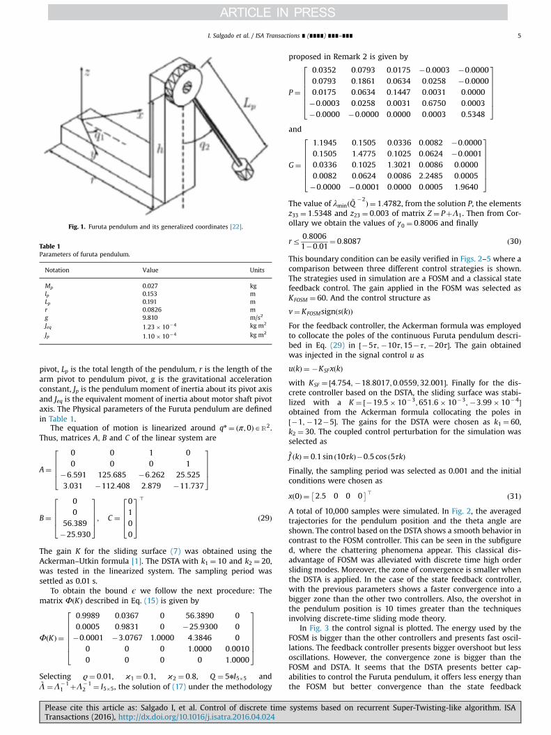
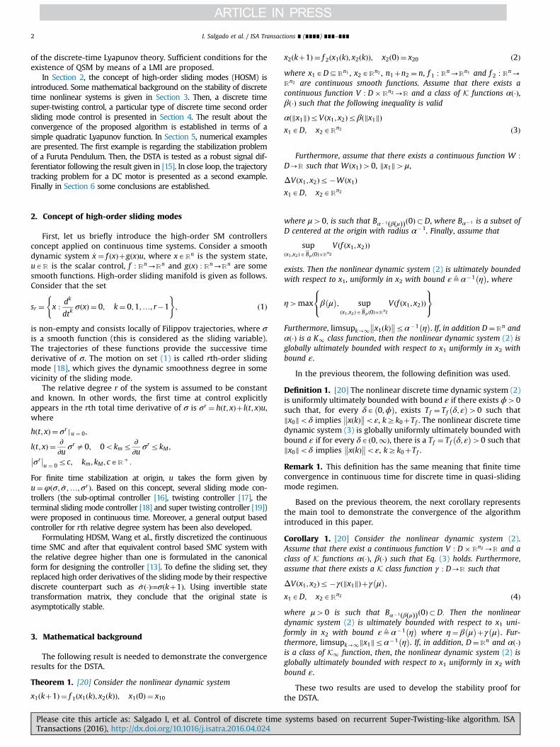
Fig. 1. Furuta pendulum and its generalized coordinates [22].

Table 1Parameters of furuta pendulum.

Notation Value Units

Mp 0.027 kglp 0.153 mLp 0.191 mr 0.0826 mg 9.810 m/s2

Jeq 1:23� 10�4 kg m2

Jp 1:10� 10�4 kg m2


pivot, Lp is the total length of the pendulum, r is the length of thearm pivot to pendulum pivot, g is the gravitational accelerationconstant, Jp is the pendulum moment of inertia about its pivot axisand Jeq is the equivalent moment of inertia about motor shaft pivotaxis. The Physical parameters of the Furuta pendulum are definedin Table 1.

The equation of motion is linearized around qn ¼ π;0ð ÞAR2.Thus, matrices A; B and C of the linear system are

A¼

0 0 1 00 0 0 1

�6:591 125:685 �6:262 25:5253:031 �112:408 2:879 �11:737

26664

37775

B¼

00

56:389�25:930

26664

37775; C ¼

0100

26664

37775

>

ð29Þ

The gain K for the sliding surface (7) was obtained using theAckerman–Utkin formula [1]. The DSTA with k1 ¼ 10 and k2 ¼ 20,was tested in the linearized system. The sampling period wassettled as 0.01 s.

To obtain the bound ϵ we follow the next procedure: Thematrix ΦðKÞ described in Eq. (15) is given by

ΦðKÞ ¼

0:9989 0:0367 0 56:3890 00:0005 0:9831 0 �25:9300 0�0:0001 �3:0767 1:0000 4:3846 0

0 0 0 1:0000 0:00100 0 0 0 1:0000

26666664

37777775

Selecting ϱ¼ 0:01, ϰ1 ¼ 0:1, ϰ2 ¼ 0:8, Q ¼ 5nI5�5 and~Λ ¼Λ�1

1 þΛ�12 ¼ I5�5, the solution of (17) under the methodology


proposed in Remark 2 is given by

P ¼

0:0352 0:0793 0:0175 �0:0003 �0:00000:0793 0:1861 0:0634 0:0258 �0:00000:0175 0:0634 0:1447 0:0031 0:0000�0:0003 0:0258 0:0031 0:6750 0:0003�0:0000 �0:0000 0:0000 0:0003 0:5348

26666664

37777775

and

G¼

1:1945 0:1505 0:0336 0:0082 �0:00000:1505 1:4775 0:1025 0:0624 �0:00010:0336 0:1025 1:3021 0:0086 0:00000:0082 0:0624 0:0086 2:2485 0:0005�0:0000 �0:0001 0:0000 0:0005 1:9640

26666664

37777775

The value of λminð ~Q�2Þ ¼ 1:4782, from the solution P, the elements

z33 ¼ 1:5348 and z23 ¼ 0:003 of matrix Z ¼ PþΛ1. Then from Cor-ollary we obtain the values of γ0 ¼ 0:8006 and finally

rr 0:80061�0:01

¼ 0:8087 ð30Þ

This boundary condition can be easily verified in Figs. 2–5 where acomparison between three different control strategies is shown.The strategies used in simulation are a FOSM and a classical statefeedback control. The gain applied in the FOSM was selected asKFOSM ¼ 60. And the control structure as

v¼ KFOSMsign s kð Þð ÞFor the feedback controller, the Ackerman formula was employedto collocate the poles of the continuous Furuta pendulum descri-bed in Eq. (29) in ½�5τ; �10τ;15�τ; �20τ�. The gain obtainedwas injected in the signal control u as

u kð Þ ¼ �KSFx kð Þwith KSF ¼ ½4:754; �18:8017;0:0559;32:001�. Finally for the dis-crete controller based on the DSTA, the sliding surface was stabi-lized with a K ¼ ½�19:5� 10�3;651:6� 10�3; �3:99� 10�4�obtained from the Ackerman formula collocating the poles in½�1; �12�5�. The gains for the DSTA were chosen as k1 ¼ 60,k2 ¼ 30. The coupled control perturbation for the simulation wasselected as

~f kð Þ ¼ 0:1 sin 10τkð Þ�0:5 cos 5τkð ÞFinally, the sampling period was selected as 0.001 and the initialconditions were chosen as

xð0Þ ¼ 2:5 0 0 0� > ð31Þ

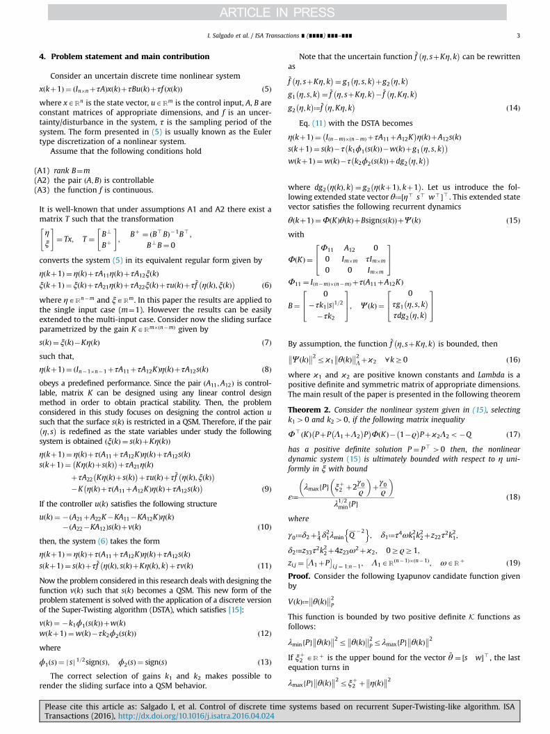
A total of 10,000 samples were simulated. In Fig. 2, the averagedtrajectories for the pendulum position and the theta angle areshown. The control based on the DSTA shows a smooth behavior incontrast to the FOSM controller. This can be seen in the subfigured, where the chattering phenomena appear. This classical dis-advantage of FOSM was alleviated with discrete time high ordersliding modes. Moreover, the zone of convergence is smaller whenthe DSTA is applied. In the case of the state feedback controller,with the previous parameters shows a faster convergence into abigger zone than the other two controllers. Also, the overshot inthe pendulum position is 10 times greater than the techniquesinvolving discrete-time sliding mode theory.

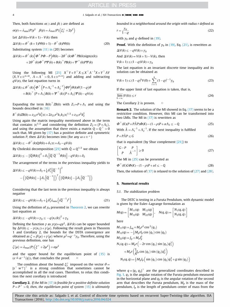
In Fig. 3 the control signal is plotted. The energy used by theFOSM is bigger than the other controllers and presents fast oscil-lations. The feedback controller presents bigger overshoot but lessoscillations. However, the convergence zone is bigger than theFOSM and DSTA. It seems that the DSTA presents better cap-abilities to control the Furuta pendulum, it offers less energy thanthe FOSM but better convergence than the state feedback





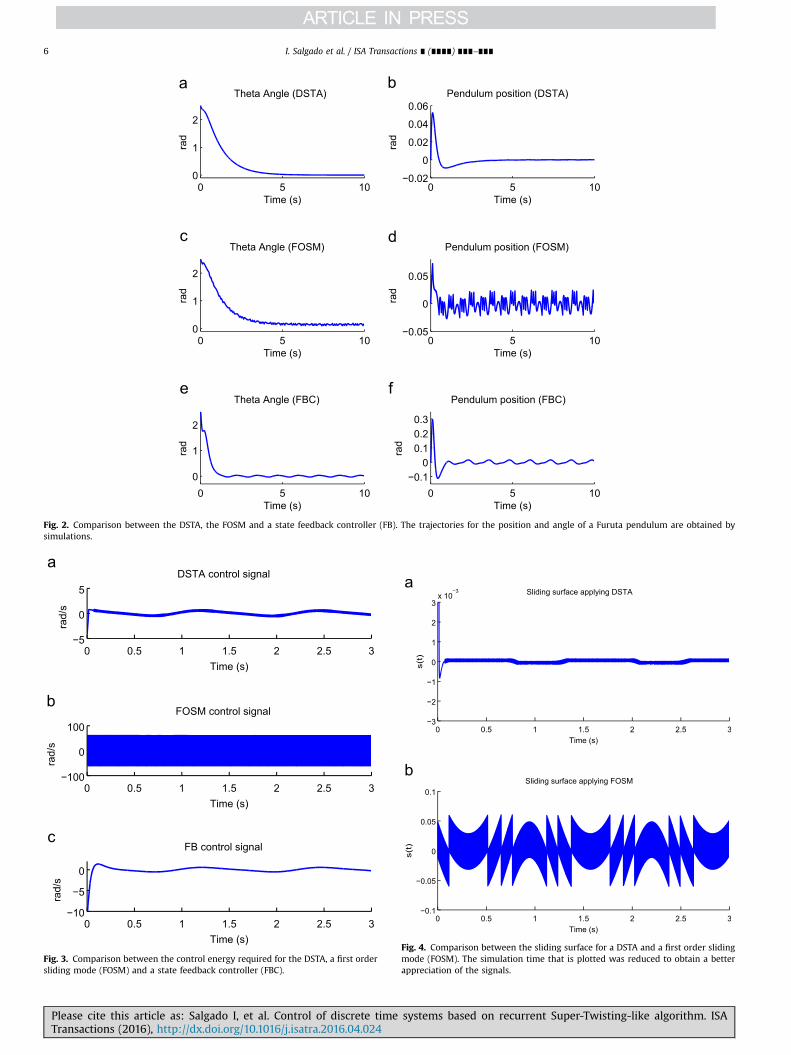
Fig. 2. Comparison between the DSTA, the FOSM and a state feedback controller (FB). The trajectories for the position and angle of a Furuta pendulum are obtained bysimulations.

Fig. 3. Comparison between the control energy required for the DSTA, a first ordersliding mode (FOSM) and a state feedback controller (FBC).

Fig. 4. Comparison between the sliding surface for a DSTA and a first order slidingmode (FOSM). The simulation time that is plotted was reduced to obtain a betterappreciation of the signals.


Please cite this article as: Salgado I, et al. Control of discrete time systems based on recurrent Super-Twisting-like algorithm. ISATransactions (2016), http://dx.doi.org/10.1016/j.isatra.2016.04.024i




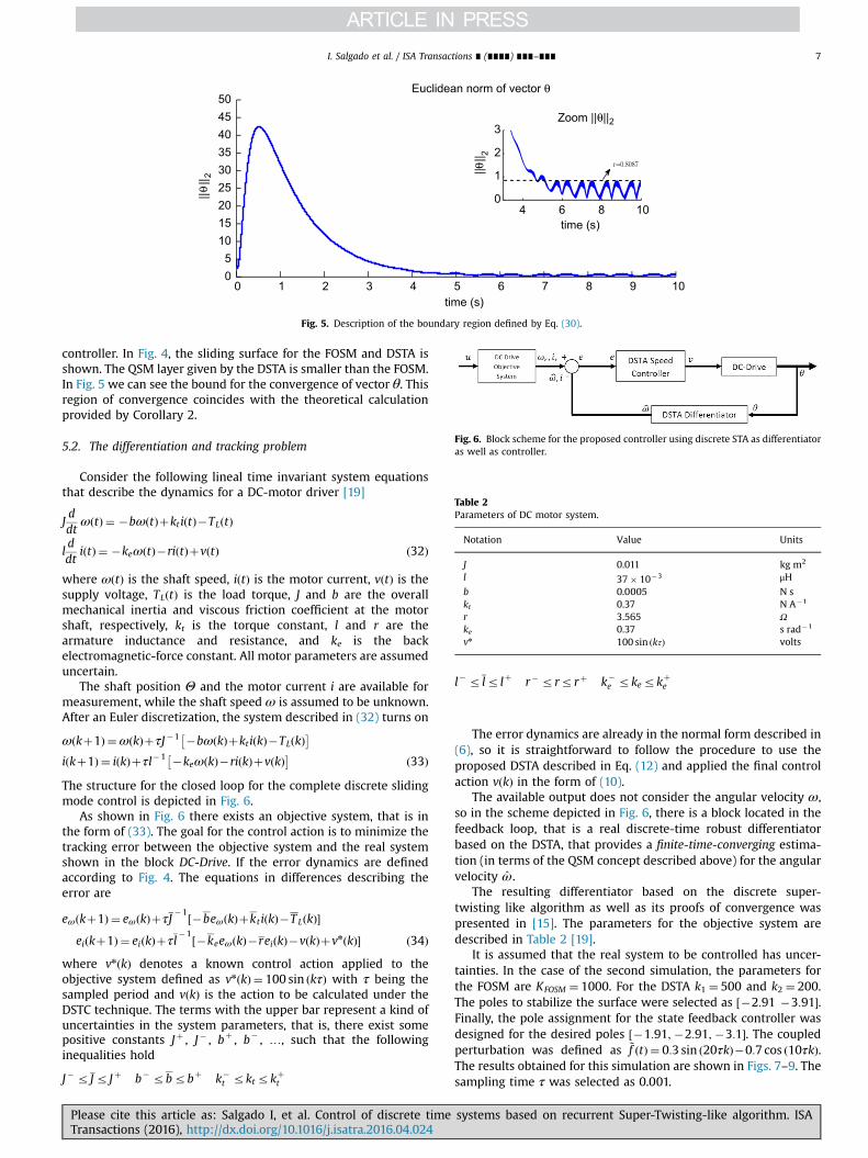
Fig. 5. Description of the boundary region defined by Eq. (30).

Fig. 6. Block scheme for the proposed controller using discrete STA as differentiatoras well as controller.

Table 2Parameters of DC motor system.

Notation Value Units

J 0.011 kg m2

l 37� 10�3 μHb 0.0005 N skt 0.37 N A�1

r 3.565 Ω

ke 0.37 s rad�1

vn 100 sin kτð Þ volts


controller. In Fig. 4, the sliding surface for the FOSM and DSTA isshown. The QSM layer given by the DSTA is smaller than the FOSM.In Fig. 5 we can see the bound for the convergence of vector θ. Thisregion of convergence coincides with the theoretical calculationprovided by Corollary 2.

5.2. The differentiation and tracking problem

Consider the following lineal time invariant system equationsthat describe the dynamics for a DC-motor driver [19]

Jddtω tð Þ ¼ �bω tð Þþkti tð Þ�TL tð Þ

lddt

i tð Þ ¼ �keω tð Þ�ri tð Þþv tð Þ ð32Þ

where ω tð Þ is the shaft speed, i tð Þ is the motor current, v tð Þ is thesupply voltage, TL tð Þ is the load torque, J and b are the overallmechanical inertia and viscous friction coefficient at the motorshaft, respectively, kt is the torque constant, l and r are thearmature inductance and resistance, and ke is the backelectromagnetic-force constant. All motor parameters are assumeduncertain.

The shaft position Θ and the motor current i are available formeasurement, while the shaft speed ω is assumed to be unknown.After an Euler discretization, the system described in (32) turns on

ω kþ1ð Þ ¼ω kð ÞþτJ�1 �bω kð Þþkti kð Þ�TL kð Þ� i kþ1ð Þ ¼ i kð Þþτl�1 �keω kð Þ�ri kð Þþv kð Þ� ð33Þ

The structure for the closed loop for the complete discrete slidingmode control is depicted in Fig. 6.

As shown in Fig. 6 there exists an objective system, that is inthe form of (33). The goal for the control action is to minimize thetracking error between the objective system and the real systemshown in the block DC-Drive. If the error dynamics are definedaccording to Fig. 4. The equations in differences describing theerror are

eω kþ1ð Þ ¼ eω kð ÞþτJ�1½�beωðkÞþktiðkÞ�T LðkÞ�

eiðkþ1Þ ¼ eiðkÞþτl�1½�keeωðkÞ�reiðkÞ�vðkÞþvnðkÞ� ð34Þ

where vnðkÞ denotes a known control action applied to theobjective system defined as vnðkÞ ¼ 100 sin kτð Þ with τ being thesampled period and vðkÞ is the action to be calculated under theDSTC technique. The terms with the upper bar represent a kind ofuncertainties in the system parameters, that is, there exist somepositive constants Jþ , J� , bþ , b� , …, such that the followinginequalities hold

J� r Jr Jþ b� rbrbþ k�t rktrkþ

t


l� r lr lþ r� rrrrþ k�e rkerkþ

e

The error dynamics are already in the normal form described in(6), so it is straightforward to follow the procedure to use theproposed DSTA described in Eq. (12) and applied the final controlaction vðkÞ in the form of (10).

The available output does not consider the angular velocity ω,so in the scheme depicted in Fig. 6, there is a block located in thefeedback loop, that is a real discrete-time robust differentiatorbased on the DSTA, that provides a finite-time-converging estima-tion (in terms of the QSM concept described above) for the angularvelocity ω̂.

The resulting differentiator based on the discrete super-twisting like algorithm as well as its proofs of convergence waspresented in [15]. The parameters for the objective system aredescribed in Table 2 [19].

It is assumed that the real system to be controlled has uncer-tainties. In the case of the second simulation, the parameters forthe FOSM are KFOSM ¼ 1000. For the DSTA k1 ¼ 500 and k2 ¼ 200.The poles to stabilize the surface were selected as ½�2:91 �3:91�.Finally, the pole assignment for the state feedback controller wasdesigned for the desired poles ½�1:91; �2:91; �3:1�. The coupledperturbation was defined as ~f tð Þ ¼ 0:3 sin 20τkð Þ�0:7 cos 10τkð Þ.The results obtained for this simulation are shown in Figs. 7–9. Thesampling time τ was selected as 0.001.





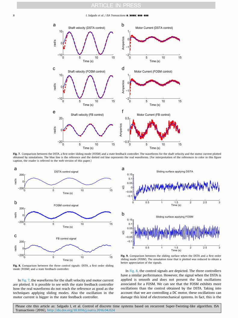
Fig. 7. Comparison between the DSTA, a first order sliding mode (FOSM) and a state feedback controller. The waveforms for the shaft velocity and the motor current plottedobtained by simulations. The blue line is the reference and the dotted red line represents the real waveforms. (For interpretation of the references to color in this figurecaption, the reader is referred to the web version of this paper.)

Fig. 8. Comparison between the three control signals: DSTA, a first order slidingmode (FOSM) and a state feedback controller.

Fig. 9. Comparison between the sliding surface when the DSTA and a first ordersliding mode (FOSM). The simulation time that is plotted was reduced to obtain abetter appreciation of the signals.


In Fig. 7, the waveforms for the shaft velocity and motor currentare plotted. It is possible to see with the state feedback controllerhow the real waveforms do not reach the reference as good as thetechniques applying sliding modes. Also the oscillation in themotor current is bigger in the state feedback controller.


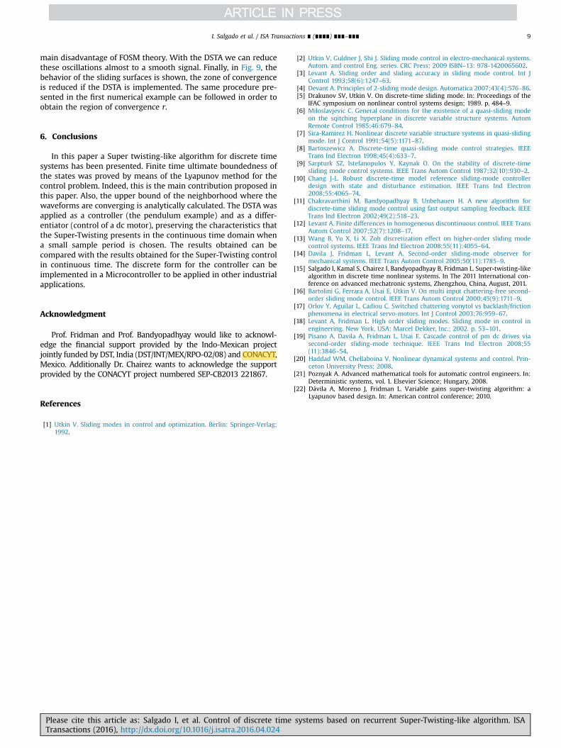
In Fig. 8, the control signals are depicted. The three controllershave a similar performance. However, the signal when the DSTA isapplied is smooth and does not present the fast oscillationsassociated for a FOSM. We can see that the FOSM exhibits moreoscillations than the control obtained by the DSTA. Taking intoaccount that we are controlling a DC motor, these oscillations candamage this kind of electromechanical systems. In fact, this is the






main disadvantage of FOSM theory. With the DSTA we can reducethese oscillations almost to a smooth signal. Finally, in Fig. 9, thebehavior of the sliding surfaces is shown, the zone of convergenceis reduced if the DSTA is implemented. The same procedure pre-sented in the first numerical example can be followed in order toobtain the region of convergence r.

6. Conclusions

In this paper a Super twisting-like algorithm for discrete timesystems has been presented. Finite time ultimate boundedness ofthe states was proved by means of the Lyapunov method for thecontrol problem. Indeed, this is the main contribution proposed inthis paper. Also, the upper bound of the neighborhood where thewaveforms are converging is analytically calculated. The DSTA wasapplied as a controller (the pendulum example) and as a differ-entiator (control of a dc motor), preserving the characteristics thatthe Super-Twisting presents in the continuous time domain whena small sample period is chosen. The results obtained can becompared with the results obtained for the Super-Twisting controlin continuous time. The discrete form for the controller can beimplemented in a Microcontroller to be applied in other industrialapplications.

Acknowledgment

Prof. Fridman and Prof. Bandyopadhyay would like to acknowl-edge the financial support provided by the Indo-Mexican projectjointly funded by DST, India (DST/INT/MEX/RPO-02/08) and CONACYT,Mexico. Additionally Dr. Chairez wants to acknowledge the supportprovided by the CONACYT project numbered SEP-CB2013 221867.

References

[1] Utkin V. Sliding modes in control and optimization. Berlin: Springer-Verlag;1992.


[2] Utkin V, Guldner J, Shi J. Sliding mode control in electro-mechanical systems.Autom. and control Eng. series. CRC Press; 2009 ISBN–13: 978-1420065602.

[3] Levant A. Sliding order and sliding accuracy in sliding mode control. Int JControl 1993;58(6):1247–63.

[4] Devant A. Principles of 2-sliding mode design. Automatica 2007;43(4):576–86.[5] Drakunov SV, Utkin V. On discrete-time sliding mode. In: Proceedings of the

IFAC symposium on nonlinear control systems design; 1989. p. 484–9.[6] Miloslavjevic C. General conditions for the existence of a quasi-sliding mode

on the sqitching hyperplane in discrete variable structure systems. AutomRemote Control 1985;46:679–84.

[7] Sira-Ramirez H. Nonlinear discrete variable structure systems in quasi-slidingmode. Int J Control 1991;54(5):1171–87.

[8] Bartoszewicz A. Discrete-time quasi-sliding mode control strategies. IEEETrans Ind Electron 1998;45(4):633–7.

[9] Sarpturk SZ, Istefanopulos Y, Kaynak O. On the stability of discrete-timesliding mode control systems. IEEE Trans Autom Control 1987;32(10):930–2.

[10] Chang J-L. Robust discrete-time model reference sliding-mode controllerdesign with state and disturbance estimation. IEEE Trans Ind Electron2008;55:4065–74.

[11] Chakravarthini M, Bandyopadhyay B, Unbehauen H. A new algorithm fordiscrete-time sliding mode control using fast output sampling feedback. IEEETrans Ind Electron 2002;49(2):518–23.

[12] Levant A. Finite differences in homogeneous discontinuous control. IEEE TransAutom Control 2007;52(7):1208–17.

[13] Wang B, Yu X, Li X. Zoh discretization effect on higher-order sliding modecontrol systems. IEEE Trans Ind Electron 2008;55(11):4055–64.

[14] Davila J, Fridman L, Levant A. Second-order sliding-mode observer formechanical systems. IEEE Trans Autom Control 2005;50(11):1785–9.

[15] Salgado I, Kamal S, Chairez I, Bandyopadhyay B, Fridman L. Super-twisting-likealgorithm in discrete time nonlinear systems. In The 2011 International con-ference on advanced mechatronic systems, Zhengzhou, China, August, 2011.

[16] Bartolini G, Ferrara A, Usai E, Utkin V. On multi input chattering-free second-order sliding mode control. IEEE Trans Autom Control 2000;45(9):1711–9.

[17] Orlov Y, Aguilar L, Cadiou C. Switched chattering vonytol vs backlash/frictionphenomena in electrical servo-motors. Int J Control 2003;76:959–67.

[18] Levant A, Fridman L. High order sliding modes. Sliding mode in control inengineering. New York, USA: Marcel Dekker, Inc.; 2002. p. 53–101.

[19] Pisano A, Davila A, Fridman L, Usai E. Cascade control of pm dc drives viasecond-order sliding-mode technique. IEEE Trans Ind Electron 2008;55(11):3846–54.

[20] Haddad WM, Chellaboina V. Nonlinear dynamical systems and control. Prin-ceton University Press; 2008.

[21] Poznyak A. Advanced mathematical tools for automatic control engineers. In:Deterministic systems, vol. 1. Elsevier Science; Hungary, 2008.

[22] Dávila A, Moreno J, Fridman L. Variable gains super-twisting algorithm: aLyapunov based design. In: American control conference; 2010.


http://refhub.elsevier.com/S0019-0578(16)30070-2/sbref1

























































Fridman

Highlight

CONACyT project 193564, and DST project DST/INT/MEX/RPO-02/2008, and DGAPA-UNAM, projects PAPIIT IN113216

Documents

Control of discrete time systems based on recurrent Super ...verona.fi-p.unam.mx/~lfridman/publicaciones/papers/ISA.pdfiva.pdf · Control of discrete time systems based on recurrent