Standard Form 298 (Rev. 8/98)

REPORT DOCUMENTATION PAGE

Prescribed by ANSI Std. Z39.18

Form Approved OMB No. 0704-0188

The public reporting burden for this collection of information is estimated to average 1 hour per response, including the time for reviewing instructions, searching existing data sources, gathering and maintaining the data needed, and completing and reviewing the collection of information. Send comments regarding this burden estimate or any other aspect of this collection of information, including suggestions for reducing the burden, to the Department of Defense, Executive Services and Communications Directorate (0704-0188). Respondents should be aware that notwithstanding any other provision of law, no person shall be subject to any penalty for failing to comply with a collection of information if it does not display a currently valid OMB control number. PLEASE DO NOT RETURN YOUR FORM TO THE ABOVE ORGANIZATION. 1. REPORT DATE (DD-MM-YYYY) 2. REPORT TYPE 3. DATES COVERED (From - To)

4. TITLE AND SUBTITLE 5a. CONTRACT NUMBER

5b. GRANT NUMBER

5c. PROGRAM ELEMENT NUMBER

5d. PROJECT NUMBER

5e. TASK NUMBER

5f. WORK UNIT NUMBER

6. AUTHOR(S)

7. PERFORMING ORGANIZATION NAME(S) AND ADDRESS(ES) 8. PERFORMING ORGANIZATION REPORT NUMBER

9. SPONSORING/MONITORING AGENCY NAME(S) AND ADDRESS(ES) 10. SPONSOR/MONITOR'S ACRONYM(S)

11. SPONSOR/MONITOR'S REPORT NUMBER(S)

12. DISTRIBUTION/AVAILABILITY STATEMENT

13. SUPPLEMENTARY NOTES

14. ABSTRACT

15. SUBJECT TERMS

16. SECURITY CLASSIFICATION OF: a. REPORT b. ABSTRACT c. THIS PAGE

17. LIMITATION OF ABSTRACT

18. NUMBER OF PAGES

19a. NAME OF RESPONSIBLE PERSON

19b. TELEPHONE NUMBER (Include area code)

13-09-2012 Final Report 01 JUN 2008 - 30 NOV 2011

Active Control of Unsteady Gasdynamics for Shock Compression and Turbulence Generation

FA9550-08-1-0333

FA9550-08-1-0333

61102F

Adonios Karpetis

Aerospace Engineering Texas A&M University College Station, TX

Air Force Office of Scientific Research 875 N Randolph St Ste 325, Rm 3112 Arlington, VA 22203

AFOSR

AFRL-OSR-VA-TR-2012-1082

Distribution A: Approved for Public Release. Unclassified, unrestricted.

An important research area in propulsion science today involves transient processes. Steady state combustion has long been studied and used in engines, but transient processes are now being examined to determine their abilities in propulsion systems. One of the main ideas for transient propulsion involve pulsed detonations, and are referred to as pulsed detonation engines (PDE). Although the theory behind their use is sound, the implementation can be quite dangerous due to the high pressures involved with their operation. A safer approach to creating the transient pressure waves may be found using pulsed supersonic flames. The present work will examine the creation of a pulsed supersonic flame through actuation of the incoming oxidizer.

U U U U 99

Adonios Karpetis

979-458-4301

Reset

1

Final Performance Report

FA9550-08-1-0333

Active Control of Unsteady Gasdynamics for Shock Compression

and Turbulence Generation

Principal Investigators:

Dr. Adonios Karpetis

Dr. Rodney Bowersox

Dr. Tamas Kalmar-Nagy

Dr. Helen Reed

Institution:

Aerospace Engineering

Texas A&M University

College Station, TX

Period of Performance:

1 June 2008 to 30 November 2011

1

1. INTRODUCTION

Propulsion science is always expanding into new areas of research. From new

areas like electromagnetic propulsion, to the more common combustion based en-

gines, every area is advancing. Supersonic combustion and propulsion are gathering

momentum as researchers strive to go faster, higher, and farther, pushing the limits

of our current knowledge of aerospace propulsion.

A more common method utilized in aerospace propulsion is the ramjet [1]. By

travelling at supersonic speeds, a shock wave forms at the inlet which works to

compress the incoming fluid. The increased pressures and temperatures obtained in

post shock conditions help to prepare a flow for downstream combustion [2]. However,

the main requirement for the ramjet, supersonic speed (M ≥ 1), can also be the

most difficult to obtain. Multiple stages are often required to achieve the supersonic

condition, at which point the ram effect continues the acceleration into higher Mach

number regimes, as made famous by the Pratt and Whitney J58 engine used on the

SR-71 Blackbird [3].

There is a possible method for mitigating the use of multiple staged engines using

one robust engine solution with transient pulsed pressure waves, as seen in Figure

1.1. The shock wave needed for combustion in a ramjet engine may be synthesized

through pulsed pressure waves. The interaction of weak pressure waves applied at

a nozzle inlet could potentially interact to form a strong shock within the duct.

This strong shock can be formed at subsonic speeds, and would prepare a flow for

combustion. This would greatly reduce the speeds needed to operate a ramjet engine

(M < 1). Other major advantages to such an engine include safety, and the lack

of moving parts which will drastically lower overall operating costs. The motivation

behind the present work is to examine the possibility of using a pulsed supersonic

flame as a generator of these weak pressure waves.

This thesis follows the style of Journal of Propulsion and Power .

2

Fig. 1.1. Proposed solution for construction and operation of a lowspeed ramjet engine. Pulsed pressure waves interact and coalesce toform a normal shock within the duct, preparing a flow for combustion.

An important research area in propulsion science today involves transient pro-

cesses. Steady state combustion has long been studied and used in engines, but

transient processes are now being examined to determine their abilities in propulsion

systems. One of the main ideas for transient propulsion involve pulsed detonations,

and are referred to as pulsed detonation engines (PDE) [4, 5]. Although the theory

behind their use is sound, the implementation can be quite dangerous due to the high

pressures involved with their operation. Pulsed jets have also been studied, mainly

for use in supersonic combustion ramjets (scramjets) [6–8]. These pulsed supersonic

jets are typically used for flow control, or for fuel injection into scramjet engines.

However, the principles used in the pulsed jets are generally related to detonation

tubes.

A safer approach to creating the transient pressure waves may be found using

pulsed supersonic flames. The present work will examine the creation of a pulsed

supersonic flame through actuation of the incoming oxidizer. The pulsed actuation

is achieved using an electromagnetic solenoid which controls the flow of air into the

combustor. With correct timing the system will ignite, providing a high pressure,

supersonic flame at the combustor exit. Other methods for pulsed air systems have

been explored, but the electromagnetic solenoid was chosen for its cost and ease of

implementation [9, 10].

3

The combustor used in the experiment is constructed using jet engine principles,

and uses a flame holder to promote turbulence and stabilize a flame. The effects of

flame holders has been well researched since the 1950s for use in jet engine config-

urations [11–13]. Additionally, a de Laval nozzle is used to accelerate the flame to

supersonic speeds. Converging-diverging nozzles have also been well documented for

use in rockets and jet engines [2, 14,15].

Information on flames is often gathered optically. Two optical methods used in

this experiment are an Intensified CCD (ICCD) and a schlieren system. Both of these

methods have been used extensively for combustion research. The ICCD is often

used in conjunction with laser based solutions for induced fluorescence, providing

measurements of molecular constituents in the flame [16, 17]. However, the present

work is more concerned with gathering photons created through chemiluminescence,

the natural emission of light from a flame. Chemiluminescence has also been detected

using ICCD systems, typically with different sets of filters applied to better resolve

the concentrations of certain species in a flame [18, 19]. The present work focuses

primarily on the qualitative aspects of the transient flame, although optical filters

can be applied to the ICCD in the future. The schlieren setup is also used extensively

in laboratories [20, 21]. A schlieren setup is appealing to combustion processes due

to the ability of the system to detect density gradients produced by both high speed

flows, and combusting gases [22,23].

The flow pattern of a supersonic jet has been observed since the early 1900s, but

is still important today. The structure of the supersonic jet can be an indication

of the performance of a nozzle, but can also be observed to understand combustible

areas within the flow [24]. The shockwave interactions for under and overexpanded

jets are well defined in literature [2, 14].

This thesis is divided into sections. Section 2 details the experimental setup used

to produce the transient supersonic flame, and the numerical model that mimics the

experimental system. Included in this section is the description of gas regulation for

4

the experimental system, as well as the design of the combustor. Additionally, the

computational model of the experimental system is described. Section 3 discusses

the design and creation of the two optical systems used to image the transient super-

sonic flame. Section 4 concludes this thesis by presenting and discussing the results

obtained both visually and computationally.

5

2. TRANSIENT SUPERSONIC FLAME APPARATUS AND SIMULATION

In what follows, the design, construction, and simulation of the transient super-

sonic flame apparatus is discussed. The combustion chamber was based on previous

work in creating miniaturized combustors for afterburner flames [25]. The present

system is a transient extension of the existing steady state device. The transient

nature was discovered when unburnt flow through the nozzle was blocked using a

thin walled obstruction [26]. The stagnation would allow a flammable mixture to

form, creating a transient flame which would burst through the obstruction. The

new device is operated transiently through the use of an electromagnetic solenoid

valve. The valve actuation is designed to mimic the blocking effect of the obstruc-

tion. Chemilluminescence is desired because it is natural light emitted from the

flame, allowing for observation without laser assistance. In terms of light emitted,

supersonic flames are not very robust. Transient flames compound this problem,

due to the small timescales in the experiment. The apparatus is simulated using

Cantera, an open source software package, providing detailed chemistry and ther-

modynamic information. The program will be used to understand the behavior of

thermochemistry within the combustion chamber throughout the transient event.

2.1 Supersonic Flame Apparatus

Due to the high pressures and temperatures that occur within the combustion

chamber, materials that were able to withstand flame conditions were required. For

this reason, brass and stainless steel components were used. These components were

selected for their ease of use, availabilty, and machineability. The thermal coefficients

of expansion between the two materials are similar, mitigating any problems inherent

in heating dissimilar metals. In addition, high temperature thread locking material

is applied to prevent any gas leaks during the combustion process.

6

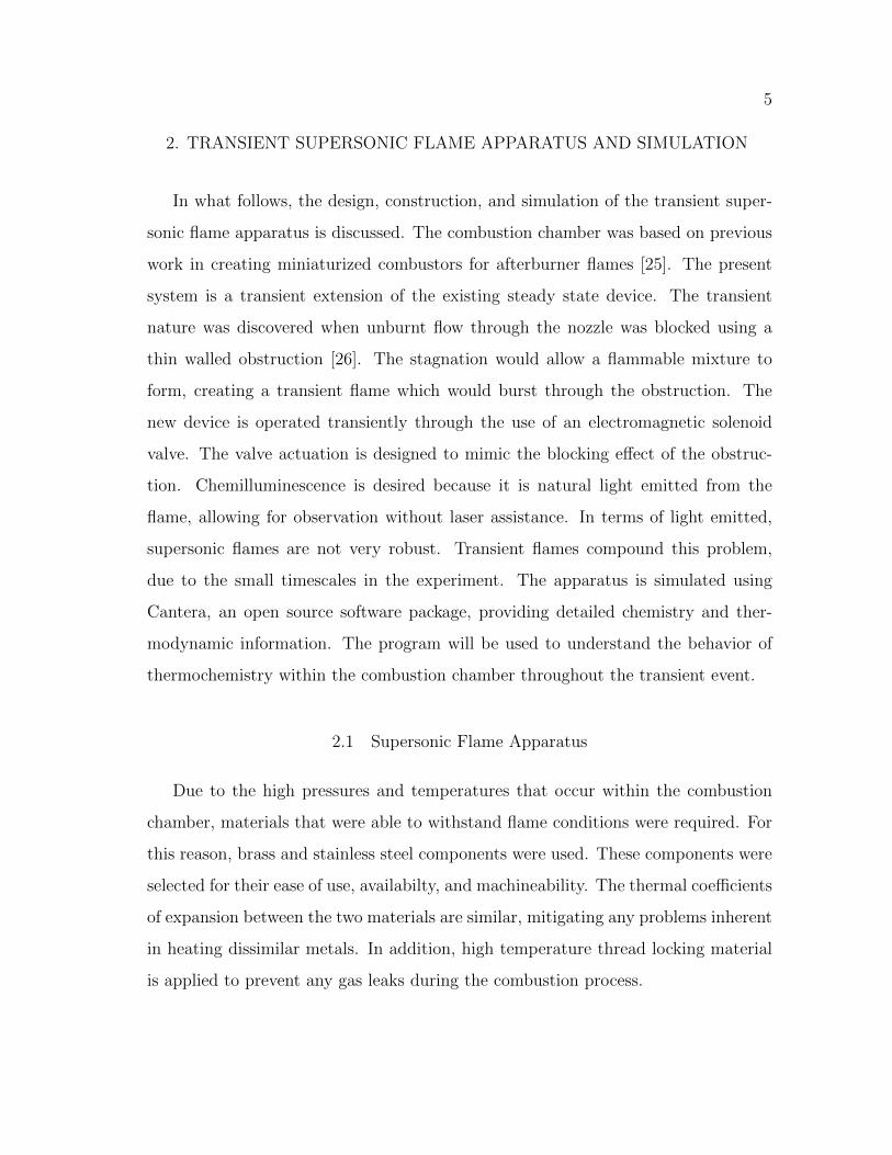
The combustion chamber features three distinct sections. The outer chamber,

the flame tube, and the nozzle, as shown in Figure 2.1. Methane is injected directly

into the central flame tube. The tube contains a bluff body stabilizer (flame holder)

combined with a spark plug in the recirculation region to initiate combustion [27].

The 90 vee-shaped bluff body occupies approximately half the area in the flame

tube and is placed directly at the center of the flow. Assuming a maximum velocity

of 10 m/s through the flame tube, and for an incompressible flow, the bluff body

obstruction woud create a pressure drop of less than 100 Pa. Therefore, the pressure

drop across the blockage is neglected due to the low velocities within the combustion

chamber. The recirculation region can be estimated as a wedge-shaped body, with a

characterized length as a parameter of bluff body height and flow velocity [13]. This

region will be discussed in Section 4.2.

The initial construction of the combustor was based on designs for vitiated-air jet

engines. Air is injected into the outer chamber via a solenoid valve, and is allowed to

Fig. 2.1. Section view of computer generated combustor assembly.

7

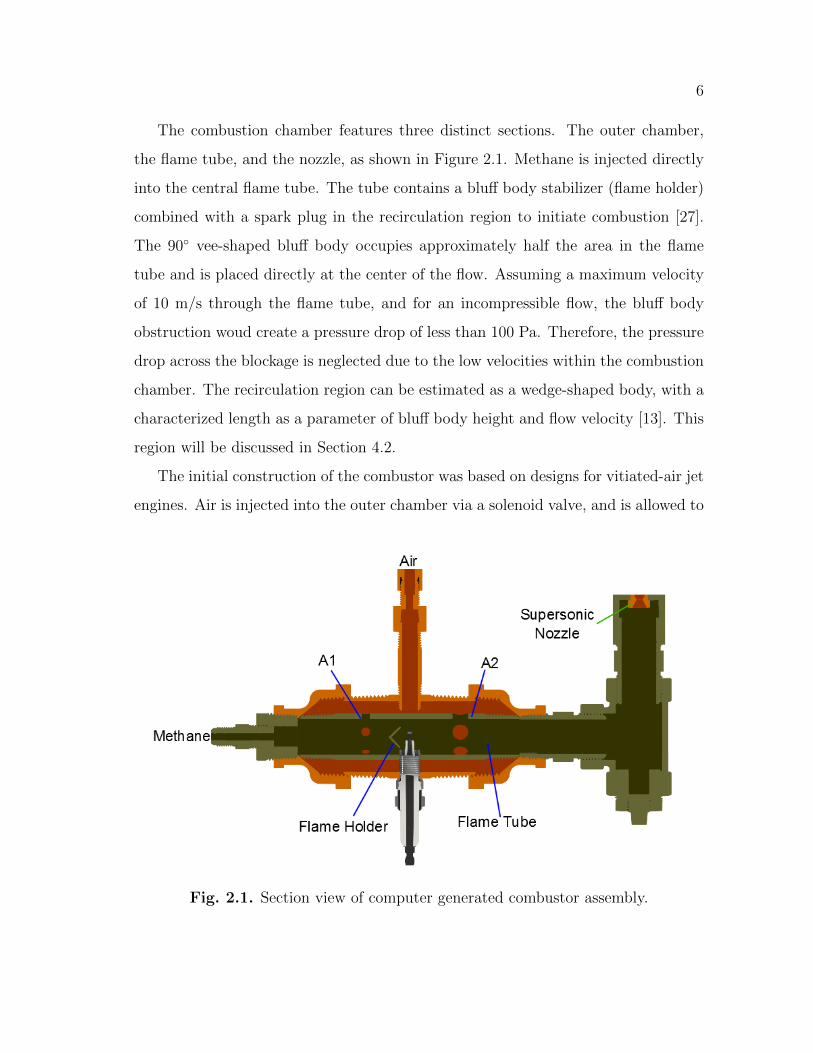
mix with the methane through two entry areas (A1 and A2). The electromagnetic

solenoid has an opening/closing time in the order of 25 ms. This relatively fast

actuation will provide the appropriate air transient for combustion. The primary

and secondary regions are a circular pattern of holes, with a secondary/primary area

ratio of 3.3, as seen in Figure 2.1. Although the air inlets were initially designed to

mimic air inlets on a jet engine, the actual operation is much different, and will be

discussed in later sections.

Mass flow rates are metered by choked orifice plates at the methane and air supply

tanks. The combination of orifices would result in a steady state equivalence ratio of

φ = 1.4, less than the upper flammability limit of 1.7 for methane [28]. However, the

transient nature of the system yields an equivalence ratio that is continually changing

throughout the actuation process. As the solenoid begins to open (t ' 0 ms), the

area restriction at the solenoid produces a choked flow. As time progresses (t > 0

ms), pressure will build within the chamber, allowing for mixing of reactant gases.

At this point, the air recirculates within the volume created by the flame holder,

mixing with the methane and allowing combustion to occur.

After ignition, the products of combustion are then accelerated downstream

through a de Laval nozzle. The de Laval nozzle expands the flow past M = 1,

producing supersonic flow at the nozzle exit. The throat diameter is the smallest

area in the combustion chamber to ensure choking after the air and fuel have been

mixed. After undergoing a slight area expansion, the reacting gases are exhausted

to the atmosphere. The ratio of exit area to throat area (ε expansion ratio in rocket

science) is 1.25. Using the following 1-D isentropic expansion equation, the Mach

number at the exit can be found.

(Aexit

Athroat

)2 =1

M2[

2

γ + 1(1 +

γ − 1

2M2)]

γ+1γ−1 (2.1)

8

where M is Mach number, Aexit and Athroat are the exit areas and nozzle throat areas,

and γ is the ratio of specific heats for the fluid [2]. The resulting Mach number at

the nozzle exit is M = 1.6.

The nozzle is constructed from superfine isomolded graphite. The properties of

graphite make it ideal for use in rocket nozzles [14]. Graphite experiences minimal

shape change when heated, making it optimall for use in the transient combustion

environment where the nozzle is constantly being quickly heated/cooled. Addition-

ally, this property ensures that heat based fracturing will not occur, mitigating the

constant replacement of nozzles. Temperatures required for the ablation and sub-

limation of graphite are in excess of 3800 K [29]. This is much higher than the

temperatures reached within the combustion chamber, as will be shown in later sec-

tions. The temperature never exceeds 2700 K, and that is observed only during

short durations throughout the transient burn. The small timescales of the transient

flame mitigate the effects of erosive burning on the nozzle area ratio (Equation 2.1).

Therefore, erosive burning of the nozzle surface is neglected due to the transient

nature of the experiment.

The spark plug used to ignite the system is driven by an ignition coil which is

charged by a 13.8V 15 Amp power supply. The key element to creating a high voltage

spark is the rapid change of current through the ignition coil. This is achieved using

a 2N3055 NPN transistor. Unlike a mechanical relay, the transistor allows for fast

changes in current flow, creating voltages in the ignition coil upwards of 15 kV,

ensuring a very energetic spark.

The various timescales of the experiment require accurate time coordination. The

system timing can be controlled using two different methods, a) through the use of

an in-house built timing circuit, or b) by using a Berkeley Nucleonics 565 pulse

generator. The first method requires a set of circuits designed around the LM555

timer integrated circuit (IC) operating in cascading monostable mode. The second

method uses a pulse generator which has an array of individually controlled channels

9

Fig. 2.2. Relative timescales used in the experiment. (A) representsthe open solenoid time (∼200 ms), and (B) is the ignition spark(∼1 ms). The experiment is initiated by a button press. The delay(τ1) determines the ignition point, and is required for allowing thereactants to mix before combustion.

through which 5 V Transistor-Transistor-Logic (TTL) signals can be generated. The

goal is to control the timescales used in the experiment. The timing revolves around

a master signal, in this case the solenoid valve. The length of the master signal

indicates the amount of time the solenoid is open for, as seen in Figure 2.2. A second

pulse is used to trigger the ignition spark. The delay time between the solenoid

closing and the spark must also be tuned to ensure combustion occurs, as will be

discussed in Section 4.1. A third trigger is needed for the image intensifier and is

described in Section 3.1.

The methane and air flows are provided by regulated tanks far upstream of the

combustor. Orifice plates are used to control the mass flow rates of the methane

and air just downstream of the pressure regulators. The orifices ensure a flammable

mixture during the ignition process. Total pressure at the regulator can be varied

between 60–120 psig for the experiment. These bounds are predetermined by ex-

perimental conditions; the solenoid valve cannot withstand upstream tank pressures

10

above 120 psig, and the combustor nozzle will not choke at a tank pressure below 60

psig, according to the result described in Equation 2.3.

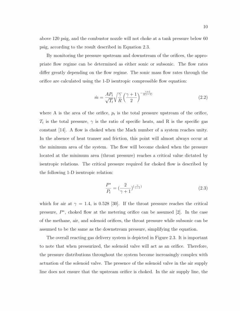
By monitoring the pressure upstream and downstream of the orifices, the appro-

priate flow regime can be determined as either sonic or subsonic. The flow rates

differ greatly depending on the flow regime. The sonic mass flow rates through the

orifice are calculated using the 1-D isentropic compressible flow equation:

m =APt√Tt

√γ

R

(γ + 1

2

)− γ+12(γ−1)

(2.2)

where A is the area of the orifice, pt is the total pressure upstream of the orifice,

Tt is the total pressure, γ is the ratio of specific heats, and R is the specific gas

constant [14]. A flow is choked when the Mach number of a system reaches unity.

In the absence of heat transer and friction, this point will almost always occur at

the minimum area of the system. The flow will become choked when the pressure

located at the minimum area (throat pressure) reaches a critical value dictated by

isentropic relations. The critical pressure required for choked flow is described by

the following 1-D isentropic relation:

P ∗

Pt

= (2

γ + 1)(

γγ−1

) (2.3)

which for air at γ = 1.4, is 0.528 [30]. If the throat pressure reaches the critical

pressure, P ∗, choked flow at the metering orifice can be assumed [2]. In the case

of the methane, air, and solenoid orifices, the throat pressure while subsonic can be

assumed to be the same as the downstream pressure, simplifying the equation.

The overall reacting gas delivery system is depicted in Figure 2.3. It is important

to note that when pressurized, the solenoid valve will act as an orifice. Therefore,

the pressure distributions throughout the system become increasingly complex with

actuation of the solenoid valve. The presence of the solenoid valve in the air supply

line does not ensure that the upstream orifice is choked. In the air supply line, the

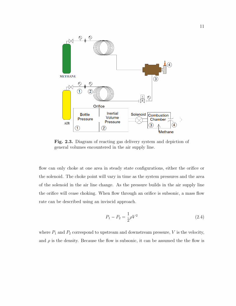
11

Fig. 2.3. Diagram of reacting gas delivery system and depiction ofgeneral volumes encountered in the air supply line.

flow can only choke at one area in steady state configurations, either the orifice or

the solenoid. The choke point will vary in time as the system pressures and the area

of the solenoid in the air line change. As the pressure builds in the air supply line

the orifice will cease choking. When flow through an orifice is subsonic, a mass flow

rate can be described using an inviscid approach.

P1 − P2 =1

2ρV 2 (2.4)

where P1 and P2 correspond to upstream and downstream pressure, V is the velocity,

and ρ is the density. Because the flow is subsonic, it can be assumed the the flow is

12

Fig. 2.4. Graph representing an example of pressure within theinertial volume during solenoid actuation. Note the separate regionsof subsonic/supersonic flow.

incompressible. Therefore, density in this case can be considered constant. Solving

for velocity, the mass flow rate can be found using the definition of mass flow rate:

m = ρV A =√

2ρ(P1 − P2)A (2.5)

where A is the area of the orifice.

The presence of a solenoid valve at the combustion chamber, which acts to quickly

start and stop the supply of air, will cause the volume between the supply tank and

solenoid valve to become pressurized. This pressurized system has an inertia that

must be taken into account when simulating the combustion process, as it will greatly

affect the combustion system pressure, as shown Figure 2.4.

Although there will be a temperature loss due to the expansion of gases through

their respective orifices, the surface area of the supply lines will ensure that enough

13

heat transfer will occur to keep the gas at ambient temperatures. The exception to

this is the mass flow rate through the nozzle, as the temperature of the combustion

chamber can not be assumed ambient at all times. The thermodynamic properties

of the combustor are calculated by the software package described in Section 2.2 to

calculate the nozzle mass flow rate.

Figure 2.4 shows the pressure distribution within the inertial volume for one of the

operating conditions of the experiment (corresponding to a tank pressure of 95 psia).

The solenoid opens at time t =0 s, causing the supersonic discharge of air due to the

relatively large choked area of the solenoid. Because the combustion chamber has a

nozzle with a small throat diameter, there will be an accumulation of pressure in the

combustion chamber. As the pressure in the chamber rises the solenoid orifice will

stop choking, causing subsonic discharge through the solenoid orifice. The lowered

pressure in the inertial volume will cause the air orifice upstream of the solenoid

to begin flowing, attempting to replenish the volume created in the air supply line.

Due to the large area of the solenoid orifice, steady state conditions would result in

choked flow through the air orifice, and subsonic flow through the solenoid. When

the solenoid begins to close at approximately t = 200 ms, the inertial air supply

volume will fill as it did before t = 0 ms, eventually reaching a steady state pressure

corresponding to the back pressure of the system, as shown in Figure 2.4.

2.2 Combustor Simulation

The combustor is simulated as a zero-dimensional well-stirred reactor (WSR)

using Cantera [31]. Cantera is a suite of object-oriented software tools used for

chemically reacting flow problems involving chemical kinetics, thermodynamics, and

transport processes [32]. The present work uses the Gas Research Institute Mecha-

nism 3.0 (GRI-Mech 3.0), which is an optimized detailed kinetic mechanism based

on experimental measurements designed to model methane-air combustion [33]. It

utilizes 325 mostly reversible reactions and 53 gas species. This work is performed

14

Fig. 2.5. Basic diagram of combustor simulation within Cantera.

using Python 2.6, an object oriented programming language with various scientific

and mathematic library packages available [34]. Comparisons of simulated reactor

based combustion experiments with Cantera have been performed, but the literature

on the topic is scarce [35]. However, the code has been validated in certain geome-

tries against experimental data [35]. The present study will use the results only in a

qualitative sense, in order to explain the observations in the experiment. Therefore,

questions of computational accuracy do not arise.

The zero dimensional model assumes that gases are instantaneously mixed, re-

gardless of the vessel size or the pressure differences and velocities across the reactor.

This introduces several discrepancies in the comparison of the experiment to the

simulation. Assumptions must be made to ensure congruency between the physical

device and the simulation. The volume of the combustor is estimated to be 120 cm3.

The overall system is modeled in Cantera as shown in Figure 2.5. The ignition event

is mimicked by injecting hydrogen atoms into the flow. The extreme reactivity of

these atoms initiates combustion. The hydrogen atoms have a profound effect on

a transient system. The mass flow rate profile for hydrogen is in the shape of a

Gaussian pulse, as a function of time. Due to the transient nature of the system, the

15

Fig. 2.6. Effect of hydrogen atom injection on a simulated steadystate system. Case A) Not enough hydrogen atoms added, no reac-tion occurs. Case C) Too many hydrogen atoms are added, resultingin an inaccurate temperature spike with reaction. Case B) The cor-rect amount of hydrogen atoms are added, resulting in a reactionwith a small transient temperature spike. Time in this case is notrelated to the times used in the rest of the figures.

characteristics of the pulse had to be carefully selected because of how it affects the

simulation, as seen in Figure 2.6. Atoms are literally added to the flow, and begin

affecting the chemistry and thermodynamic properties of the gas as soon as they are

injected.

As shown in Figure 2.1, there are two injection regions for air into the system (A1,

A2), which necessitate the use of two different combustor volumes for the simulation.

However, the complexities that the two area ratios of the combustor pose led to the

adaptation of the single volume model shown in Figure 2.5. Although Eularian

simulations have been performed using bluff body stabilized flames, the transient

nature of the calculation will assume a Lagrangian moving flame volume, and will

be discussed in Section 4.2 [36]. The final combustion products are exhausted to an

infinite reservoir, mimicking atmospheric conditions. The supply tanks are located

40 feet away from the experiment, necessitating the inclusion of large inert volumes

for which the air and methane can occupy before flowing into the combustor. The

16

Fig. 2.7. Representation of the solenoid orifice area as a function oftime. The 25 ms opening and closing timescale is depicted linearlyfor the opening and closing actuation.

role of the inertial volume is important, as pressure effects heavily influence the

experiment, and therefore must be accounted for within the simulation. Although

there is an inertial volume in the methane supply line, the effects of this volume are

neglected. The relative orifice area of the methane is small enough to ensure that

it will always be choked, and will therefore be providing a constant mass flow rate.

For this reason, the inertial volume in the methane supply line is neglected.

Because the solenoid is a mechanical system, there is a physical timescale asso-

ciated with opening and closing the device. This timescale is approximated to be

25 ms. During this period, the solenoid orifice area is changing, greatly affecting

the mass flow rate (msol) through the device. In an ideal case, the solenoid would

open instantaneously, allowing air to move through it at a rate proportional to the

upstream pressure, as shown in Figure 2.4. In reality, the 25 ms opening time will

create a “pulse” discussed in later sections. This pulse is the result of the high

pressure air in the inertial air supply volume being discharged into the combustion

chamber. The solenoid connecting the high pressure inertial volume to the combus-

17

tor will be choked until the pressure in the inertial supply volume drops below the

critical value for choking, described by Equation 2.3. When the solenoid is no longer

choked, the mass flow rate (msol) will be equivalent to the choked value of the air

orifice (mAir). The area change of the solenoid is modeled in time, as shown in Figure

2.7. The opening and closing times are described as linear slopes for simplification

of the problem. The area described is used in Equations 2.2 and 2.5 to calculate the

mass flow rate of the solenoid (msol).

18

3. EXPERIMENTAL TECHNIQUES

Imaging the transient flame phenomenon poses many difficulties due to the small

timescales present in the experiment, and the generally low light conditions in the

flame. Unlike laser-induced methods which generate photons, the present work relied

on chemiluminescence, i.e. the emission of light as a result of chemical reactions.

These complications were dealt with via two different methods which were applied

to the transient flame.

3.1 The Image Intensifier

The main benefit of the image intensifier the ability to amplify the number of

photons emanating from an experiment. This experiment used a 3rd generation (Gen

III) ITT Night Vision image intensifier (FS9910C). An image intensifier has three

primary components within its housing: the photocathode, the photoanode, and the

microchannel plate (MCP) [37]. In this particular intensifier, gallium arsenide is used

as the photoelectric material in the photocathode, and a P43 phosphor was used for

the photoanode [38].

The quantum efficiency (QE) of an image intensifier is based on the photoelectric

materials utilized, and is defined as:

QE =#Photoelectrons

#Photons(3.1)

Gen III image intensifiers are known for their high QE, which can be in excess of

50% depending on the observed wavelength and the properties of the photoelectric

material used [37]. The spectral response curve of the gallium arsenide photocathode

is nearly flat for wavelengths of 450 nm–850 nm, ideal for imaging any flame in the

visible spectrum.

19

Fig. 3.1. Diagram of a Microchannel Plate (MCP), reproduced withpermission from Hamamatsu Photonics [37].

The MCP is constructed using a glass wafer, which contains thousands of small

glass tubes or slots, as shown in Figures 3.1 and 3.2 [37]. As the electrons enter

the electrically charged MCP and ricochet through the channels, they are multiplied

by making contact with the sidewalls of the tube [37]. The number of electrons

generated is proportional to the voltage differential across the MCP. The outgoing

electrons then strike the photoanode which emits photons to be captured either by

eye or photodetector. The gain of the system is adjustable by altering the voltage

differentials of either the photocathode, or the MCP.

Fig. 3.2. Diagram of the operation of an image intensifier.

20

The photocathode is the most important component in regards to the transient

supersonic flame. Timing is brought into the system by the methods mentioned in

Section 2.1. The photocathode must be quickly pulsed to achieve optimal results. If

it is not pulsed quickly enough, a “smearing” effect will appear in the photos taken.

However, pulsing too fast could limit the amount of entering light, causing dim or

noisy photos. There is a balance that must be found experimentally. The optimal

gating value was found to be between 1–3 ms. Other experiments typically utilize

laser induced methods for increasing light levels, providing intensifier gates as low

as 2 ns [16]. Although the image intensifier was capable of gates as low as 20 ns,

the low light from the experiment required the larger gate to capture the event with

minimal noise.

High voltages are provided by an in-house built power supply, which utilizes a

high voltage pulser for the photocathode, and a steady state high voltage power

supply for the differential voltages across the MCP and photoanode, as shown in

Figure 3.3. A 24V DC power supply provides energy for both the steady state

high voltage power supply and the high voltage pulser. The high voltage pulser

can be tuned between -500 V and -900 V, providing an extra gain control on the

photocathode if desired. It is triggered by a TTL signal provided by either of the

signal generators listed in Section 2.1, allowing precisely timed gating of the image

intensifier. The steady state power supply provides an 8 kV potential, which was

split using a voltage divider network, providing separate voltages for the MCP and

photoanode. Low current needed to be ensured to keep from burning out the power

supply, so resistance values in the MΩ range were chosen for use in the divider

network. The fractions in Figure 3.3 show relative values that were used.

3.2 Charge-Coupled Device

CCDs operate using electronic shift registers to move an electrical charge out of

the CCD pixels and into an A/D converter for digitizing the signal obtained [39].

21

Fig. 3.3. Schematic of image intensifier power supply unit. Thepulser has a variable resistor that provides voltage tuning of the neg-atively charged pulse. The voltage divider resistor network utilizesMΩ valued resistors, depicted as fractions to convey relative resistorvalues. The provided voltages apply to the intensifier depicted inFigure 3.2.

CCDs are often used for scientific purposes in large part due to their typically high

quality photo-imaging abilities, pixel binning options, and cooling capabilities. Most

CCDs present a high quantum efficiency of 60% or more (90% for state of the art

CCD systems), with uniform and reproducible images, making them ideal for the

laboratory environment.

A Santa Barbara Instruments Group (SBIG) Pixcel 255 (ST-5) astronomical de-

tector was used to obtain intensified images of the emerging flame fronts. The im-

ages were gathered through CCDOps, a proprietary imaging software created by

SBIG [40]. The ST-5 has a resolution of 320x240 pixels, with a pixel size of 10x10

µm [41]. The ST-5 was chosen because of its thermoelectric cooling abilities, mount-

ing style, software support, and picture quality, all of which is related to the original

purpose of astronomical imaging. Additionally, astronomical CCDs typically offer

high signal to noise ratios (SNR = S/N), comparable to scientific CCDs.

22

The noise N of any shot-limited signal can be related to the actual signal, rep-

resented as photon counts P by the formula N ∼ P 1/2. The SNR for such a simple

system then follows as SNR ∼ P 1/2, stating that an increase in signal levels will

create a small increase in SNR [38]. However, physical systems contain more sources

of noise which can be accounted for in the following equation:

SNR =PQτ

[(P + B)Qτ + Dτ +N2A/D]1/2

(3.2)

where P is the rate of arriving photons (s−1), B is the arrival rate of background

photons (s−1), D is the electron generation rate from thermal effects on the CCD

(dark current, in s−1), NA/D is the read-out noise that is generated during the Analog-

to-Digital conversion process (unitless), Q is the quantum efficiency of the detector

(unitless), and τ is the exposure time of the image [38]. An image intensifier increases

the output gain of incoming photons, which can be represented in the SNR as G:

SNR =GPQτ

[(P + B)GQτ + Dτ +N2A/D]1/2

(3.3)

Minimizing the noise sources is essential to improving the quality of the images

obtained. At least two of the noise sources can be attenuated. The background

photons are eliminated in three ways, by operating within a light-tight area (reduc-

ing B), by using short exposure times on the CCD (reducing τ), and by gating the

image intensifier (also reducing τ). Dark current noise can be minimized using ther-

moelectric cooling, which is pre-installed on the ST-5 (reducing D). The camera can

cool the CCD to a steady state value of -17C, drastically increasing the SNR of the

camera. Pixel-binning is not supported by the ST-5, therefore the read-out noise

cannot be eliminated.

23

Fig. 3.4. Two dimensional representation of the coupling of theimage intensifier to the CCD. Note the honeycomb shapes in theoutput image. These cells are unique to Gen III intensifiers. Aprotective film is placed on the photocathode to prevent electronsfrom flowing back into the photocathode. The honeycomb shapesare from the metal grid that supports the protective film.

3.3 Optical Relay

Typically, an image intensifier is fitted to an imaging system by a fiber optic plate.

In this work, an optical relay consisting of multiple lenses was used instead. Despite

the higher efficiencies obtained through fiber optic coupling, the optical relay was

chosen due to its cost savings, versatility in the lab environment, and the inherent

difficulty of applying a fiber optic plate to the intensifier output window. However,

several problems arise when attempting to couple the intensifier to a CCD.

Lenses typically mount to a CCD using specifically designed connectors that vary

between manufacturers. For this reason, Nikon lenses were exclusively used to ensure

congruency when mounting components. Every lens has a specified register, which

is the distance from the mounting ring to the focal point of the lens. This value

is extremely precise and must be respected, as any errors will greatly influence the

focusing of the optical system. Nikon lenses have a register of 46.5 mm with an F

style optical mount [42].

The image intensifier provides an input/output window for observation, neces-

sitating careful coupling of the Nikon lenses. A schematic of the system is shown

in Figures 3.4 and 3.5. The f number of a lens is defined as f/D , where f is the

24

CCD detector

2 x 50 mmf /1.4

50 mmf /1.2

intensifier

Fig. 3.5. Three dimensional representation of the optical relay system.

focal length of the lens, and D is its diameter. More light can be captured using a

lower f number, because of the larger solid angle of collection. The amount of light

transmitted through a lens will decrease with the square of the f number [43]. A

Nikon prime f/1.2 is used as a collecting lens on the front of the system, as it will

capture the most light for the intensifier. The f/1.2 must be placed exactly 46.5 mm

away from the input window of the intensifier to ensure proper focus of the system.

The image from the output window of the intensifier is relayed to the CCD

through two f/1.4 lenses placed front-to-front, as seen in Figures 3.4 and 3.5. The

front-to-front method helps to cancel the geometric abberations introduced when

working with spherical lenses. When planar light enters a spherical lens, the wave-

fronts at the exit become spherical [44]. Naturally, running the spherical wavefronts

backwards through the same lens reverses the process, producing a planar image once

more. The planar image is focused onto the focal plane array (FPA), completing the

relay. The f/1.4 lenses are focused at infinity, allowing for 1:1 image conjugation

from the intensifier to the CCD.

25

Fig. 3.6. Relative timescales used in the experiment. (A) representsthe open solenoid time (∼200 ms), (B) is the ignition spark (∼1 ms),and (C) is the activation duration of the image intensifier (∼1 ms).The experiment is initiated by a button press. The delay (τ1) deter-mines the ignition point, and is required for allowing the reactantsto mix before combustion. The second delay (τ2) determines whichphase of the flame is captured. τ2 = 28 ms corresponds to the flameemergence from the nozzle.

3.4 Intensifier Timescale

The assembly of the intensifier system adds complexity to the timing system de-

scribed in Section 2.1. The intensifier will require a gated signal in order to trigger

the device, as discussed in Section 3.1. Figure 2.2 must now be updated to reflect

the addition of the ICCD. The optimal trigger value for the photocathode pulser was

experimentally determined to be between 1–3 ms. In order to capture the chemilu-

minescence from the emerging flame, a delay time is needed for the intensifier. The

flame will take a certain amount of time to travel through the combustor and finally

arrive at the nozzle, and will be discussed in Section 4.2. When it arrives at the

nozzle, the ICCD can then capture the light. The flame travel time, or intensifier

delay, was experimentally determined to be ≈ 28 ms. This new delay time can now

be added to the timing system, expressed in Figure 3.6.

26

3.5 Intensified Image Data

Fig. 3.7. Singular flame imaging results in separate phases of flowobserved at same delay times. Initial conditions inside combustorchanges overall flame timescales, posing difficulties in time matchingintensified images.

Intensified imaging was an overall success, but there were several problems en-

countered when using the system. Due to the limitations of the ST-5 CCD, the pic-

ture frame rate is much greater than 1 second. This means that unlike the schlieren

data, multiple phases of a single transient flame cannot be captured. Instead, sin-

gle images can be taken of separate flames, and then stitched together to create an

overall progression of the flame. However, the experiment is sensitive to initial con-

ditions, and therefore the flame does not perform exactly the same way with each

trial. For example, two pictures of separate flames obtained with the same delay time

after ignition are shown in Figure 3.7. Although taken at the same delay time, they

do not correspond exactly due to the minute flow differences within the experiment

(i.e. solenoid timescales, turbulent interactions from A1 and A2, etc.). Therefore,

intensified flame progressions are not considered. Instead, the examination will be

limited to singular images of singular flames.

Lastly, varying the CCD exposure time and intensifier pulse time can give very

different results. The methods for minimizing noise in the system, stated in Section

3.2, are demonstrated in Figure 3.8. The picture on the right is the result of a

long exposure of the CCD coupled with a short pulse from the intensifier. The

chemilluminescence of the flame is visible, but there is increased noise in the photo.

Referring to Equation 3.3, a long exposure of the CCD will result in an increase

27

Fig. 3.8. Imaging difficulties using image intensifer. The left figureis an example of providing a large gate to the intensifier, resultingin a smeared photo with overexposed regions. The right figure theresult of long exposure times of the CCD, causing increased noise inthe image obtained.

of τ , B, and D, while keeping P the same. What results is an increase in noise,

lowering the overall SNR of the system. The left picture is the result of increasing

the gate width provided to the image intensifier. By doing so, a smearing effect is

produced on the flame. All data regarding the supersonic jet structure is lost due to

the increased gain of the photons emitted during combustion.

3.6 Schlieren Imaging

Light, when moving through a volume of air, will be refracted depending on

the inhomogeneity in the density gradients and the resulting index of refraction

[23]. Schlieren is a property of any transparent medium, including solids, liquids,

and gases, which result from temperature changes, high speed flows, or the mixing

of dissimilar fluids, amongst many other possible causes [23]. Essentially, density

variations of some order (ρ, 5ρ, 52ρ) will produce visible streaks in a schlieren

system [23]. Schlieren can provide an observer with a qualitative understanding of

the complexities present in a flow. In the present work, the supersonic structure of

the transient flame is observed using a schlieren setup, and is captured using a high

speed camera.

The high speed cameras used in the schlieren portion of the results are the Casio

EX-FH25 and the Fujifilm HS10, both of which render video at 1000 frames per

28

Fig. 3.9. Depiction of a Z-type schlieren setup. Light generated at(A) is focused onto the parabolic mirror (B). (B) collimates the lightthrough the test section, arriving at the second parabolic mirror (C).(C) focuses the incoming light to a point at (D). The knife edge actsto block light rays that were refracted through the test section. Lightray (1) did not encounter an obstruction, and so passes through tothe camera (E). Light ray (2) is refracted by the obstruction, and isconsequently blocked by the knife edge at point (D).

second with a resolution of 224x64 pixels. This equates to one frame per millisec-

ond, providing detailed views of the supersonic flow structure emanating from the

combustor. Both cameras utilize a new complementary metal–oxide–semiconductor

(CMOS) FPA. This new technology offers high speed imaging at a low cost.

There are several ways to construct a schlieren system, but the Z-type system was

chosen due to its simplicity, as seen in Figure 3.9 [45]. The Z-type system utilizes two

concave mirrors to collimate/decollimate the light rays. The system operates by first

condensing light through a pinhole, which is then focused onto the first parabolic

mirror (B). The mirror is located exactly 17.5 in away from the pinhole, causing the

reflected light to be collimated. The collimated light is then focused by a second

mirror (C) into a single point (D). At the focal point of the second mirror, a knife

edge is used to cut off any light that is refracted due to gradients in the flow, as

represented in Figure 3.9 by (2). The position of the knife edge is important, as it

29

controls which gradient directions will be amplified. In this experiment, due to the

fast exposure times of the high speed cameras, a great deal of light was required to

observe the transient flame. The light source utilized was a 150W fiber-optic haloid

lamp condensed through a microscope lens.

The mirrors are angled at 8, providing an incoming and outgoing beam angle of

16. The Z-type schlieren system will always have some error in the focused beam

due to astigmatism [23]. Astigmatism is the failure to focus a beam to a point, and

results from symmetry breaking [23]. It should be noted that with the mirrors used

in the Z-type system, any angle of the reflected light will produce astigmatic error.

The problem cannot be rectified, by definition of the optical geometry. However, the

abberations due to astigmatism are small and are not overtly visible in the gathered

data.

30

4. RESULTS AND SUMMARY

In this chapter, results will be presented from the zero dimensional computation,

schlieren imaging, and the ICCD. A relationship is made between the computational

model and the schlieren high speed images. This is done by analysis of timescales

within both systems. Additionally, flame properties are tracked through time and

space using a Lagrangian reference frame. This allows flame properties to be analyzed

just prior to the nozzle entrance. Flow properties through the nozzle are calculated

using one dimensional isentropic flow relations. The calculation of thermodynamic

properties downstream of the nozzle allow a comparison to be made between the

schlieren images and the combustor model.

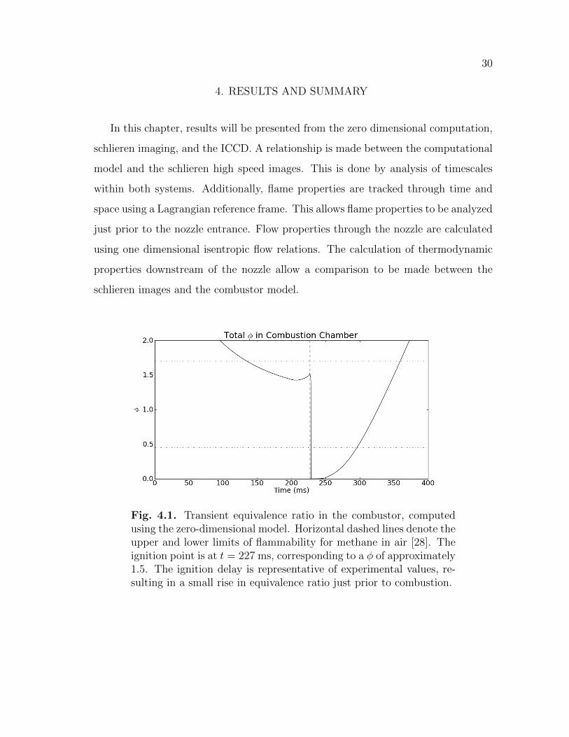
Fig. 4.1. Transient equivalence ratio in the combustor, computedusing the zero-dimensional model. Horizontal dashed lines denote theupper and lower limits of flammability for methane in air [28]. Theignition point is at t = 227 ms, corresponding to a φ of approximately1.5. The ignition delay is representative of experimental values, re-sulting in a small rise in equivalence ratio just prior to combustion.

31

4.1 Transient Zero-Dimensional Thermochemistry in the Combustor

Several timescales are important during the operation of the transient flame sys-

tem. The process is initiated at t = 0 ms by opening the solenoid. The length of time

that the solenoid is open is crucial in creating a flammable mixture for the system,

as seen in Figure 4.1. The equivalence ratio φ is determined by the overall mass

ratio of fuel and oxidizer in the combustor as it relates to the stoichiometric mass

ratio. The fuel-air mass ratio in the chamber is dynamic, and is computed using

the mass fractions reported by Cantera for each time step. When the experiment

begins, the chamber is initially filled with methane, corresponding to an unbounded

(infinite) equivalence ratio. Gradually, as air enters the chamber, the equivalence

ratio will decrease until t = 200 ms. The equivalence ratio at t = 200 ms is based on

the choked orifice values listed in Section 2.1 and corresponds to a local minimum

of a transient case. If the calculation continued indefinitely, a steady state value of

φ = 1.4 would be reached.

At t = 200 ms, the solenoid begins to close. Ignition occurs at t = 227 ms. The

lack of incoming air will result in φ increasing slightly, just prior to combustion. The

27 ms delay in ignition is needed in the experiment for gas mixing, but the WSR

used by Cantera does not need this delay time. It is included in the simulation for

ensuring as much possible continuity in the comparison between the experimental

and simulated timescales. During combustion, the methane and oxygen are being

consumed, causing the equivalence ratio to drop to zero. Because the methane

continues flowing into the combustor and the solenoid is closed, the the lack of air

in the system will create a second unbounded equivalence ratio at time t 250ms.

When a flame is present, the fuel and oxidizer will be depleted, leading momen-

tarily to φ = 0. This duration between t ≈ 230 ms and t ≈ 255 ms, shown in Figure

4.1, shows the extent of the flame. Experimentally, the ignition point is determined

by inspection of the flame, and audible cues. Ignition at a φ closest to one will result

32

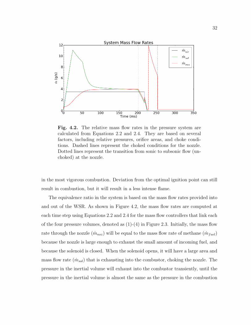
Fig. 4.2. The relative mass flow rates in the pressure system arecalculated from Equations 2.2 and 2.4. They are based on severalfactors, including relative pressures, orifice areas, and choke condi-tions. Dashed lines represent the choked conditions for the nozzle.Dotted lines represent the transition from sonic to subsonic flow (un-choked) at the nozzle.

in the most vigorous combustion. Deviation from the optimal ignition point can still

result in combustion, but it will result in a less intense flame.

The equivalence ratio in the system is based on the mass flow rates provided into

and out of the WSR. As shown in Figure 4.2, the mass flow rates are computed at

each time step using Equations 2.2 and 2.4 for the mass flow controllers that link each

of the four pressure volumes, denoted as (1)-(4) in Figure 2.3. Initially, the mass flow

rate through the nozzle (mnoz) will be equal to the mass flow rate of methane (mfuel)

because the nozzle is large enough to exhaust the small amount of incoming fuel, and

because the solenoid is closed. When the solenoid opens, it will have a large area and

mass flow rate (msol) that is exhausting into the combustor, choking the nozzle. The

pressure in the inertial volume will exhaust into the combustor transiently, until the

pressure in the inertial volume is almost the same as the pressure in the combustion

33

Fig. 4.3. Depiction of the possible mixing solution, allowing for aflammable mixture to be present at time of ignition.

chamber. When the inertial volume pressure lowers, the air orifice will become choked

(mair), providing a constant mass flow rate until such time that the solenoid closes.

The interplay between all of the mass flow rates and volumes is performed by

Cantera, where the choke conditions and mass flow rates are checked at each step,

and updated for the next step. This allows a qualitative model to be produced

based on simple assumptions, such as inviscid flow when subsonic, and isentropic

flow when supersonic. The criterion for whether or not the nozzle chokes is based on

the incoming mass flow rates for the system. If the incoming mass is lower than the

outgoing mass, then the nozzle will not be choked. Additionally, if a large pressure

and temperature increase occurs due to combustion, then the nozzle will choke. The

two choke points are indicated in Figure 4.2 by dashed lines. In the same figure, the

subsonic flow points are denoted by dotted lines.

One of the problems faced when implementing a zero-dimensional model is the

assumption of perfectly mixed gases. The zero-dimensional model cannot capture

gradients in space and mixing. When two gases are inserted into the reactor, the cal-

culation considers them instantly and perfectly mixed. In a steady state calculation,

this may not pose a problem. However, the transient behavior of the experiment is

34

heavily dependent on mixing time, implying that a mixing characteristic time must

be accounted for. This mixing time was experimentally found to be approximately

27 ms. This means that in the experiment, the ignition is delayed after the solenoid

is closed by approximately 27 ms. This is reflected in the simulation as well, although

there are repercussions for delaying the ignition, as shown in Figure 4.1.

When the experiment is initiated, gas flows into the combustion chamber and is

allowed to mix with the methane in the flame tube through areas A1 and A2, as shown

in Figure 2.1. If the flow were to be acting in steady state, then the mixture would

never ignite, due to the ratio of A1 and A2 and the metering orifice areas described.

The equivalence ratio near the spark plug would exceed the limits of combustion,

causing a failed ignition. However, the transient system ignites. This phenomenon

can be explained due to the large turbulence effects generated by the flame holder

boundary layer, and the sharp corners the flow encounters moving through A1 and

A2. Figure 4.3 illustrates the turbulent mixing occurring near the flame holder. The

flame holder provides a recirculation region in which the methane and air can mix,

allowing for a flammable mixture to be created. Additionally, the swift movement of

incoming air will result in an impinging jet through A1 and A2, causing more air to

enter the recirculation region. For a brief moment, the mixture becomes flammable,

but only in a transient configuration.

The graph in Figure 4.4 details temperature within the combustor as a function

of time. The temperature remains relatively constant within the system until the ig-

nition point at t = 227 ms. There is a minor temperature rise at t ≈ 40 ms due to the

sudden accumulation of mass in the combustion chamber. At ignition, the combustor

temperature experiences a sharp increase due to chemical energy release. Because

the air supply begins to decrease at t = 200 ms, the high temperature provided by

reactions cannot be sustained with the diminishing oxygen levels. Therefore, the

temperature within the combustor undergoes a decrease as the reactions cease to

take place. What results is a gradual return to steady state, ambient levels (t 250

35

Fig. 4.4. Time evolution of the temperature profile within the com-bustor. The grayed-out portion relates to the time at which the flameparcel reaches the nozzle, exhausting out of the combustor.

ms) with no incoming air flow. Given enough time, the system would return to the

exact state observed at t = 0 ms.

The chemistry of the flame can be quantified by analyzing the molecular makeup

of the combustor gases as they change through time and space. Only major gas

species are shown, although there are 53 different species used by the GRI-3.0 reaction

mechanism. As discussed in Section 2.2, hydrogen atoms are used to ignite the flow,

and are therefore extremely important in determining the state of combustion. The

initial hydrogen addition is provided by a Gaussian pulse. This pulse reaches its

maximum amplitude at t = 227 ms, attempting to mimick the ignition used in the

experiment. The actual ignition time between the experiment and simulation will

vary slightly, due to the methods in which they are each ignited. The experiment

is ignited using a spark plug, which operates very quickly. However, igniting a flow

in Cantera is done through hydrogen atoms, which will need time to react with the

flow before providing combustion. This small reaction delay can be seen in Figure

4.5. The reaction delay in the simulation is approximately 1 ms.

36

Fig. 4.5. Depiction of major mole fractions within the combustionchamber as a function of time. The rich flame (φ ≈ 1.5) will result inincomplete combustion, producing excess levels of CO. The dashedline indicates the maximum mass flow rate of pulsed hydrogen atoms(mH). Full reaction is observed approximately 1 ms after the max-imum of the provided pulse. The grayed-out portion relates to thetime at which the flame reaches the nozzle, exhausting out of thecombustor.

37

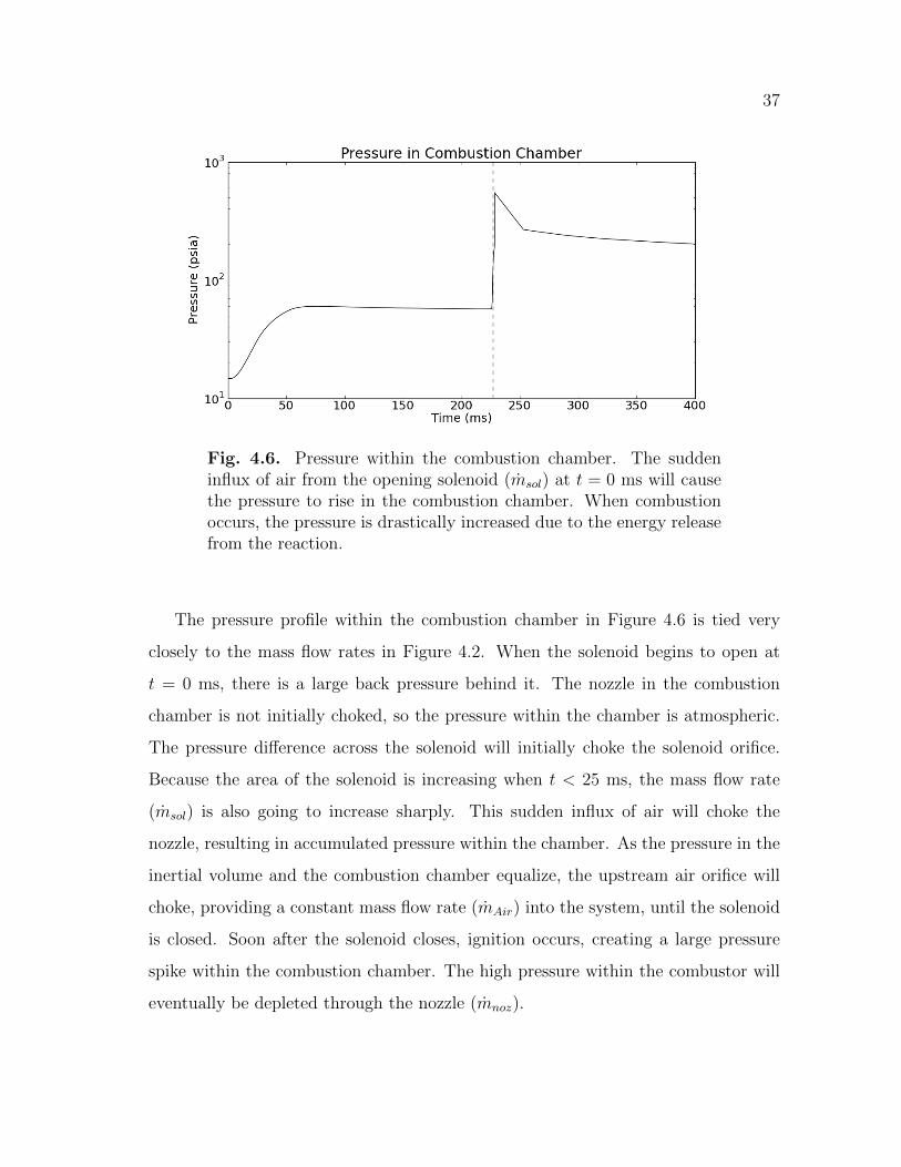
Fig. 4.6. Pressure within the combustion chamber. The suddeninflux of air from the opening solenoid (msol) at t = 0 ms will causethe pressure to rise in the combustion chamber. When combustionoccurs, the pressure is drastically increased due to the energy releasefrom the reaction.

The pressure profile within the combustion chamber in Figure 4.6 is tied very

closely to the mass flow rates in Figure 4.2. When the solenoid begins to open at

t = 0 ms, there is a large back pressure behind it. The nozzle in the combustion

chamber is not initially choked, so the pressure within the chamber is atmospheric.

The pressure difference across the solenoid will initially choke the solenoid orifice.

Because the area of the solenoid is increasing when t < 25 ms, the mass flow rate

(msol) is also going to increase sharply. This sudden influx of air will choke the

nozzle, resulting in accumulated pressure within the chamber. As the pressure in the

inertial volume and the combustion chamber equalize, the upstream air orifice will

choke, providing a constant mass flow rate (mAir) into the system, until the solenoid

is closed. Soon after the solenoid closes, ignition occurs, creating a large pressure

spike within the combustion chamber. The high pressure within the combustor will

eventually be depleted through the nozzle (mnoz).

38

4.2 Lagrangian Flame Progress

In order to link the transient zero dimensional model to experiment conditions, it

is essential to account for the time the flame spends in the combustor before exiting

the nozzle. If the time at which the flame exits the nozzle can be defined, then a

direct comparison can be made between the simulation and the experiment regarding

the temperature and flame composition downstream of the nozzle.

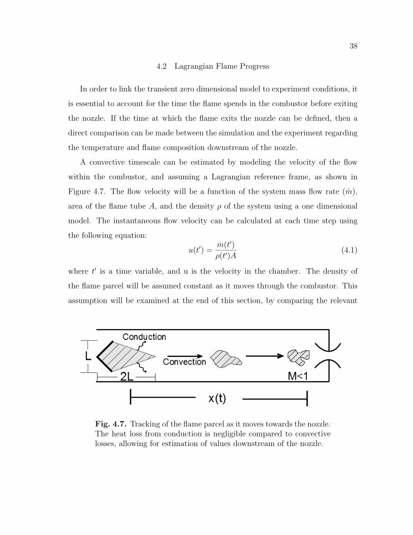
A convective timescale can be estimated by modeling the velocity of the flow

within the combustor, and assuming a Lagrangian reference frame, as shown in

Figure 4.7. The flow velocity will be a function of the system mass flow rate (m),

area of the flame tube A, and the density ρ of the system using a one dimensional

model. The instantaneous flow velocity can be calculated at each time step using

the following equation:

u(t′) =m(t′)

ρ(t′)A(4.1)

where t′ is a time variable, and u is the velocity in the chamber. The density of

the flame parcel will be assumed constant as it moves through the combustor. This

assumption will be examined at the end of this section, by comparing the relevant

Fig. 4.7. Tracking of the flame parcel as it moves towards the nozzle.The heat loss from conduction is negligible compared to convectivelosses, allowing for estimation of values downstream of the nozzle.

39

timescales. By integrating the velocity equation with time, the distance that the

fluid parcel moves can be computed:

x(t) =∫ t

0u(t′)dt =

∫ t

0

m(t′)

ρ(t′)Adt′ (4.2)

where x(t) is the distance traveled by the fluid parcel. The distance dflame required

for the fluid parcel to travel from the ignition spark to the nozzle entrance is known

from the geometry of the combustor. Therefore, by monitoring the value of x(t) and

t at each time step during the integration of Equation 4.2 and halting the calculation

when x(t) = dflame, the convective timescale of the model is found. The convective

timescale for the simulation is calculated to be t = τ2 ≈ 25 ms. This value agrees

well with observed experimental values, as will be discussed in Section 4.4.

During the progression of the flame, it will be susceptible to heat loss from con-

duction through the combustor. The losses would complicate the model, as added

heat loss effects are not currently considered in the simulation. Therefore, it is pru-

dent to estimate whether the losses from conduction are prominent. If the flame can

be convected to the nozzle faster than heat can be lost due to conduction, then the

flame computed by the model can be directly linked to the experiment. The relative

timescale of conduction can be approximated using dimensional analysis of thermal

diffusivity (α). The units of α are m2/s, indicating a need for a relative length scale

(l) and a characteristic timescale (τc), and can be related as:

α =l2

τc(4.3)

The length scale can be determined using the geometry of the fluid volume (V)

created by the flame holder, as shown in Figure 4.7. For the relatively low velocities

within the combustor, this fluid parcel volume (V) can be estimated as a function of

the flame holder geometry, in this case being obstruction height (L in Figure 4.7) [13].

This recirculation volume is based on experimental data compiled from Edelman,

40

and is estimated to extend approximately two obstruction heights downstream (2L

in Figure 4.7) [13]. Therefore, the size of the fluid parcel volume is known. The

length scale l for the thermal diffusivity can then be defined as l ≈ V 1/3.

The Sutherland model can be used to approximate the thermal diffusivity of the

fluid parcel as it undergoes combustion:

αburn

αo

= (T

To)1.7 (4.4)

where αo is the thermal diffusivity of the unburned gas, α is the high temperature

diffusivity, To is the unburned temperature, and T is the temperature of the burning

gas [46]. The thermal diffusivity of a gas αo can be related to the kinematic viscosity

νo as αo ∼ νo. Therefore, the Sutherland model can be used to estimate a thermal

diffusivity for the high temperature fluid parcel. Using Equation 4.3 in conjunction

with newly defined length scales l and the high temperature thermal diffusivity αburn,

the timescale τ can be estimated as:

τ =V 2/3

αburn

(4.5)

Equation 4.5 provides an approximation of the characteristic diffusion (conduction)

time through the fluid volume shown in Figure 4.7. The characteristic conduction

time is calculated to be τc ≈ 100 ms.

The difference between the conductive timescale (τc ≈ 100 ms) and convective

timescales (t = τ2 ≈ 30ms) is very large (τc > τ2). This means that the losses

due to conduction will be negligible compared to the speed at which the flame is

convected downstream to the nozzle. Therefore, conductive losses to the system may

be disregarded and the density may be considered constant.

Equation 4.2 connects time from the WSR model to distance traveled from the

ignition source in the experiment. With this relation, one may substitute distance

for time in the simulation and obtain the results based on distance traveled, rather

41

Fig. 4.8. Distance evolution of the temperature profile within thecombustor. Zero distance corresponds to ignition at the flame holder.The grayed-out portion relates to the where the nozzle is located.This is the distance at which the flame reaches the nozzle, exhaustingout of the combustor.

than time. Figure 4.8 details an example of this substitution, showing temperature

change with distance as the flame parcel moves through the combustor towards the

nozzle. The grayed-out areas indicate the point at which the flame parcel reaches

the nozzle, both temporally and spatially, and should be considered as the point at

which the flame exits the combustor. Therefore the data past this point should not

be considered. The downward slope of the temperature indicates that the flame is

cooling down before it gets to the nozzle. This is caused by several reasons. The

pressure in the combustor is dropping drastically at this point, which will lower the

other parameters inside the combustor, based on the ideal gas law. Additionally, the

flame is reacting while moving towards the nozzle. The reaction began very rich, so it

will not be able to sustain reaction. Therefore, the flame will not be able to provide

enough energy to keep the temperature up. This can be seen in Figure 4.9. The

chemical composition of the flame is also changing through space. The rich flame is

42

Fig. 4.9. Depiction of the mole fractions throughout combustion asdistance traveled by the flame. Zero distance corresponds to ignition.The grayed-out portion relates to the where the nozzle is located.This is the distance at which the flame reaches the nozzle, exhaustingout of the combustor.

starting to extinguish when it reaches the nozzle, shown by the increase in methane.

If the reaction were still taking place, the methane would be in the process of being

consumed. Because it is rising, the reaction must be slowing down.

One shortcoming of using the Lagrangian approach within a WSR lies in the idea

of the flame parcel being an “open system”. If the fluid parcel were truly moving

in the combustor with speed equal to the surrounding flow, outside gases would

not be entering the parcel, as is indicated in Figure 4.9. However, if considered

for qualitative purposes it is applicable to the experiment. The ability to connect

the timescales of the experiment to the WSR is valuable information, as it can be

applied to many other simulations. Transforming a zero-dimensional model into a

one-dimensional model is especially useful for transient problems, as it can help to

describe the properties of a system as it evolves through space, and not just time.

43

Fig. 4.10. Relative timescales used in the experiment. (A) rep-resents the open solenoid time (∼200 ms), (B) is the ignition spark(∼1 ms), and (C) is the duration of activation of the image intensifier(∼1 ms). τ0 is the initiation of the experiment, signified by a buttonpress. The first delay (τ1) determines the ignition point, and the sec-ond delay (τ2) determines which phase of the flame is captured. τ3 isfrom the Lagrangian approximation and corresponds to τ2.

Finally, Figures 2.2 and 3.6 can be updated to include the newly calculated travel

time of the simulated flame, as shown in Figure 4.10. This value corresponds directly

to the delay set by the ICCD. Experimentally, the flame travel time is found to be 28

ms, as indicated in Figure 4.10 by τ2. The Lagrangian approximation calculates the

flame travel time to be 25 ms (τ3), providing good correlation between the simulation

and the experiment.

44

4.3 One Dimensional Nozzle Expansion

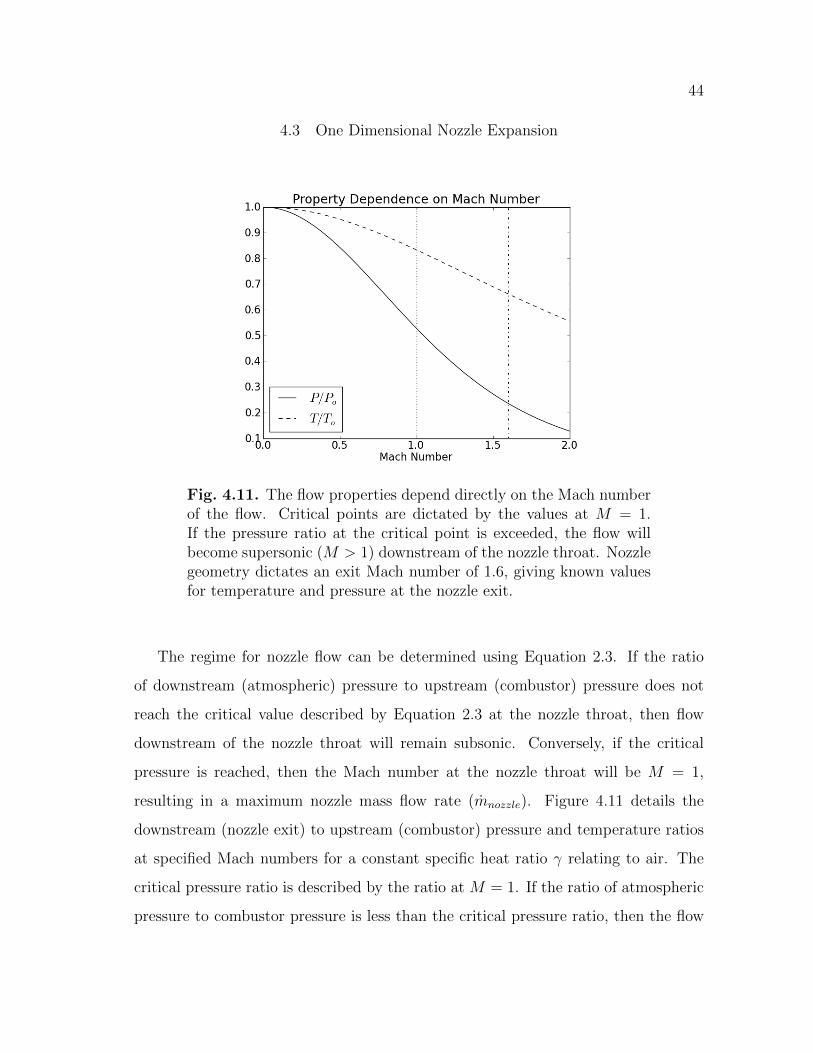
Fig. 4.11. The flow properties depend directly on the Mach numberof the flow. Critical points are dictated by the values at M = 1.If the pressure ratio at the critical point is exceeded, the flow willbecome supersonic (M > 1) downstream of the nozzle throat. Nozzlegeometry dictates an exit Mach number of 1.6, giving known valuesfor temperature and pressure at the nozzle exit.

The regime for nozzle flow can be determined using Equation 2.3. If the ratio

of downstream (atmospheric) pressure to upstream (combustor) pressure does not

reach the critical value described by Equation 2.3 at the nozzle throat, then flow

downstream of the nozzle throat will remain subsonic. Conversely, if the critical

pressure is reached, then the Mach number at the nozzle throat will be M = 1,

resulting in a maximum nozzle mass flow rate (mnozzle). Figure 4.11 details the

downstream (nozzle exit) to upstream (combustor) pressure and temperature ratios

at specified Mach numbers for a constant specific heat ratio γ relating to air. The

critical pressure ratio is described by the ratio at M = 1. If the ratio of atmospheric

pressure to combustor pressure is less than the critical pressure ratio, then the flow

45

Fig. 4.12. Computed pressure at the nozzle exit during transientflame simulation. The discontinuity at t ≈ 230 ms and t ≈ 255ms is the result of switching between subsonic and supersonic flowregimes. The initial choked behavior (t < 200 ms) corresponds toan overexpanded jet. The pressure rise from combustion creates anunderexpanded jet at nozzle exit. A brief region of subsonic flow isobserved between 200 ms < t < 230 ms. The dashed line representsatmospheric pressure.

will reach supersonic speeds past the nozzle throat. It is assumed that due to the

small size of the nozzle used in the experiment there will be no shock waves present

in the nozzle. Additionally, isentropic flow can be assumed if the expansion process is

both adiabatic and reversible [2]. Therefore, once the supersonic regime is obtained

downstream of the nozzle throat the pressure and temperature at the nozzle exit will

be dependent entirely on the combustor conditions. In the case of subsonic flow, it is

assumed the exit pressure and temperatures are approximately equal to the ambient

conditions downstream of the nozzle.

The expansion of a flow through a choked nozzle can be assumed isentropic (ds

= 0) in the absence of strong waves or reaction. It is assumed, based on the size

and contour of the nozzle, that there will be no separation within the nozzle, and

46

therefore no shock waves. For this model, it is also assumed that the chemistry

of reaction is frozen through the nozzle [14]. This approximation ensures there is

no entropy change due to reaction within the flow. These assumptions allow one

dimensional isentropic equations to be used to predict the values for temperature

and pressure at the nozzle exit. The pressure at the nozzle exit is shown in Figure

4.12. Pressure and temperature are determined using the one dimensional isentropic

nozzle equations:P

Po

= (1 +γ − 1

2M2)

−γγ−1 (4.6)

T

To= (1 +

γ − 1

2M2)−1 (4.7)

where P0 is the chamber pressure, P is the nozzle exit pressure, To is the temperature

in the combustor, which is assumed at stagnation conditions, and T is the nozzle exit

temperature [2]. The exit Mach number is known from Section 2.1, and γ is computed

at each time step by Cantera. The initial choked condition from Figure 4.2 results in

a combustor pressure that is slightly less than 4 atmospheres. When isentropically

expanded using Equation 4.6, the pressure at the nozzle exit will be slightly lower

than atmospheric. This is characteristic of an overexpanded jet. Ideally, a nozzle

is most efficient when Pexit = Patmospheric. When Pexit < Patmospheric, the jet is

overexpanded by the nozzle. Conversely, if Pexit > Patmospheric, the jet is not expanded

enough, or underexpanded.

Figure 4.12 details the exit pressures calculated in the simulation. As discussed,

the nozzle will choke very early in the simulation. What results is an overexpanded

jet during the first choked region, until t ≈ 200 ms. When the solenoid begins to

close, the incoming mass flow rates to the combustor (msol and mfuel) cannot sustain

the choked condition, and so the nozzle will become subsonic. This is indicated in

the figure from t = 200 ms to t ≈ 230 ms. Since the flow is ignited at t = 227

ms, the pressure and temperature in the combustion chamber will rise dramatically,

as calculated by Cantera in Figures 4.4 and 4.6. The conditions experienced by

47

Fig. 4.13. Computed temperature at the nozzle exit during transientflame simulation. The greyed-out region pertains to temperaturesnot observed at the nozzle due to the convective timescales withinthe combustor. The discontinuity at t = 255 ms is the result ofswitching from a supersonic regime to a subsonic regime, as describedby Equation 4.7.

the combustor during reaction will choke the nozzle a second time, resulting in an

underexpanded jet, calculated from the isentropic flow relations. As the temperature

and pressure of the system is quickly exhausted through the nozzle, the nozzle will

no longer be choked, resulting in atmospheric exit pressures (t > 255 ms). The

discontinuity in the pressure profile is from the sudden transformation of a subsonic

flow to a supersonic flow. Although in reality this transition would be a smoother

curve as the flow would need time to accelerate, it would still be a relatively fast

transition. Therefore, it is a good approximation of the transformation from subsonic

to supersonic flow.

The same assumptions used in calculating the nozzle exit pressure also apply

to calculating temperature. The temperature at the nozzle exit can therefore be

computed using Equation 4.7. The grayed-out portion of the nozzle exit temperature

profile in Figure 4.13 is data not observed in the experiment, because the flame

48

parcel has not yet reached the nozzle. Therefore the temperatures calculated before

this time will not be observed experimentally. The temperature computed at the

exit is based directly on the combustor temperature. As discussed already, the

zero dimensional model that is used to compute the reactor is transformed using

Lagrangian particle tracking. In this work, the assumption is made that the flame

parcel exiting the combustor will have properties very close to the one predicted by

the program.

Figure 4.13 depicts is the simulated temperature profile at the nozzle exit based

solely on the combustor temperature, and the choked condition. The discontinuities

at t = 228 ms and t = 255 ms are from the instantaneous switching of a subsonic to

supersonic regime, and from a supersonic to subsonic regime, respectively. When the

nozzle is not choked, the nozzle exit temperature is approximated as the combustor

temperature. When the flow is choked, the exit temperature is calculated using

Equation 4.7.

It is also important to note that pressure will act quickly within the combustor,

and temperature will have the effect of a delay based on the timescale found in Sec-

tion 4.2. Pressure is distributed through the combustor using pressure waves which

travel at the speed of sound. Temperature, however, is communicated through diffu-

sion, conduction, convection, etc. The temperature “flowing” through the combustor

will be mainly dictated by the convection, or fluid velocity, within the combustion

chamber. The pressure, however, can be assumed within the model to be acting on

the nozzle immediately.

4.4 Supersonic Flame Behavior

A supersonic flow downstream of a nozzle will have a defined structure at the

nozzle exit based on gas dynamics, and can be seen in Figures 4.14 and 4.15. An

overexpanded jet is observed when the pressure at the nozzle exit is less than the

surrounding atmospheric pressure [2]. What results is a series of diamond patterns

49

Fig. 4.14. Transient flame experiment captured by a high speedcamera in conjunction with a schlieren system. (A) - Solenoid fullyclosed. (B) - Ignition.

50

Fig. 4.15. Continued schlieren system imaging. (C) - Flame beginsto emerge from nozzle. (D) - Most vigorous flame. (E) - Entrainmentbegins. (F) - Jet becomes subsonic.

Fuel

Air

51

caused by shock wave interactions in the flow. The shock waves form when the su-

personic flow meets the free boundary of a quiescent flow. Because pressure across

the boundary must be conserved, an oblique shock wave will form at the exit. These

oblique shocks emanate from all points of the nozzle circumference, eventually meet-

ing at the centerline of the flow. At this point they will reflect, hitting the free

boundary. The new reflection will consist of expansion fans, which will behave in a

similar fashion, continuing the diamond pattern until coalescing into oblique shocks

once more. This pattern will continue until enough energy is lost and the flow be-

comes subsonic at all points [2]. An underexpanded jet will have a similar shockwave

structure, only the process will begin with expansion fans, which will reflect into

oblique shock waves. For this experiment, an inviscid, isentropic flow model is as-

sumed.

Figures 4.14 and 4.15 detail the results of the schlieren experiment using the high

speed CMOS camera. As discussed in Section 2.1, the CMOS camera frame rate is

1000 Hz, providing one frame per millisecond. The camera used does not possess the

ability to be triggered. This complicates the analysis of the transient flame because

there is no set starting point to the data. Therefore, the task of analyzing the data

falls entirely on the interpretations of the experimenter. Through examination of

the images, the following events were found. Prior to (A) in Figure 4.14, the flow is

overexpanded, resulting in very small shockwave interactions. At (A), the solenoid

is fully closed, allowing the nozzle to stop choking. Ignition occurs at (B), beginning

the convection of the flame through the combustor. As described in Section 4.2, the

flame will require a convective time to reach the nozzle. The flow remains subsonic

through the nozzle until (C) in Figure 4.15. At (C) the flame is beginning to emerge

from the combustor, and the nozzle is choked. (D) shows the most vigorous point

of the flame, manifested as an underexpanded jet. At (E), the high speed, high

temperature flow begins to entrain surrounding fluid, causing a “sheathing” effect

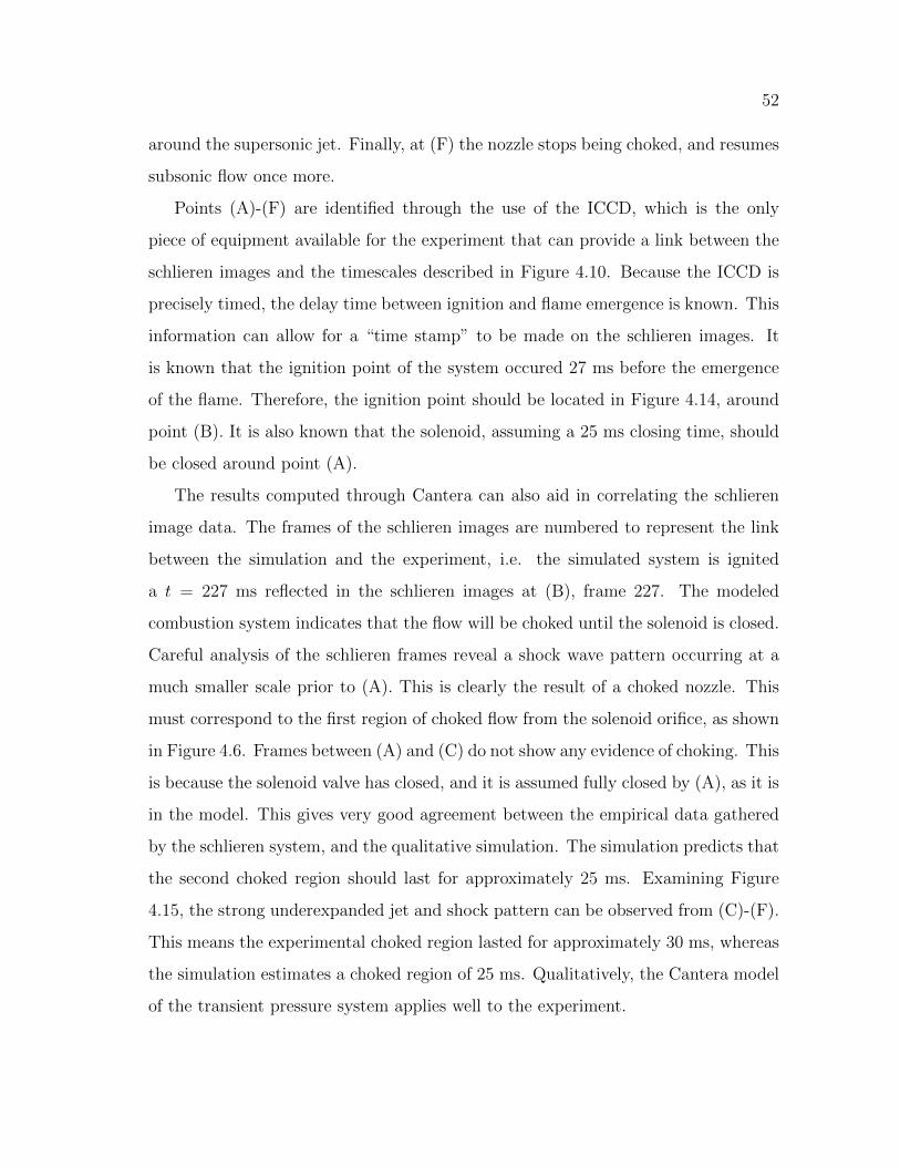
52

around the supersonic jet. Finally, at (F) the nozzle stops being choked, and resumes

subsonic flow once more.

Points (A)-(F) are identified through the use of the ICCD, which is the only

piece of equipment available for the experiment that can provide a link between the

schlieren images and the timescales described in Figure 4.10. Because the ICCD is

precisely timed, the delay time between ignition and flame emergence is known. This

information can allow for a “time stamp” to be made on the schlieren images. It

is known that the ignition point of the system occured 27 ms before the emergence

of the flame. Therefore, the ignition point should be located in Figure 4.14, around

point (B). It is also known that the solenoid, assuming a 25 ms closing time, should

be closed around point (A).

The results computed through Cantera can also aid in correlating the schlieren

image data. The frames of the schlieren images are numbered to represent the link

between the simulation and the experiment, i.e. the simulated system is ignited

a t = 227 ms reflected in the schlieren images at (B), frame 227. The modeled

combustion system indicates that the flow will be choked until the solenoid is closed.

Careful analysis of the schlieren frames reveal a shock wave pattern occurring at a

much smaller scale prior to (A). This is clearly the result of a choked nozzle. This

must correspond to the first region of choked flow from the solenoid orifice, as shown

in Figure 4.6. Frames between (A) and (C) do not show any evidence of choking. This

is because the solenoid valve has closed, and it is assumed fully closed by (A), as it is

in the model. This gives very good agreement between the empirical data gathered

by the schlieren system, and the qualitative simulation. The simulation predicts that

the second choked region should last for approximately 25 ms. Examining Figure

4.15, the strong underexpanded jet and shock pattern can be observed from (C)-(F).

This means the experimental choked region lasted for approximately 30 ms, whereas

the simulation estimates a choked region of 25 ms. Qualitatively, the Cantera model

of the transient pressure system applies well to the experiment.

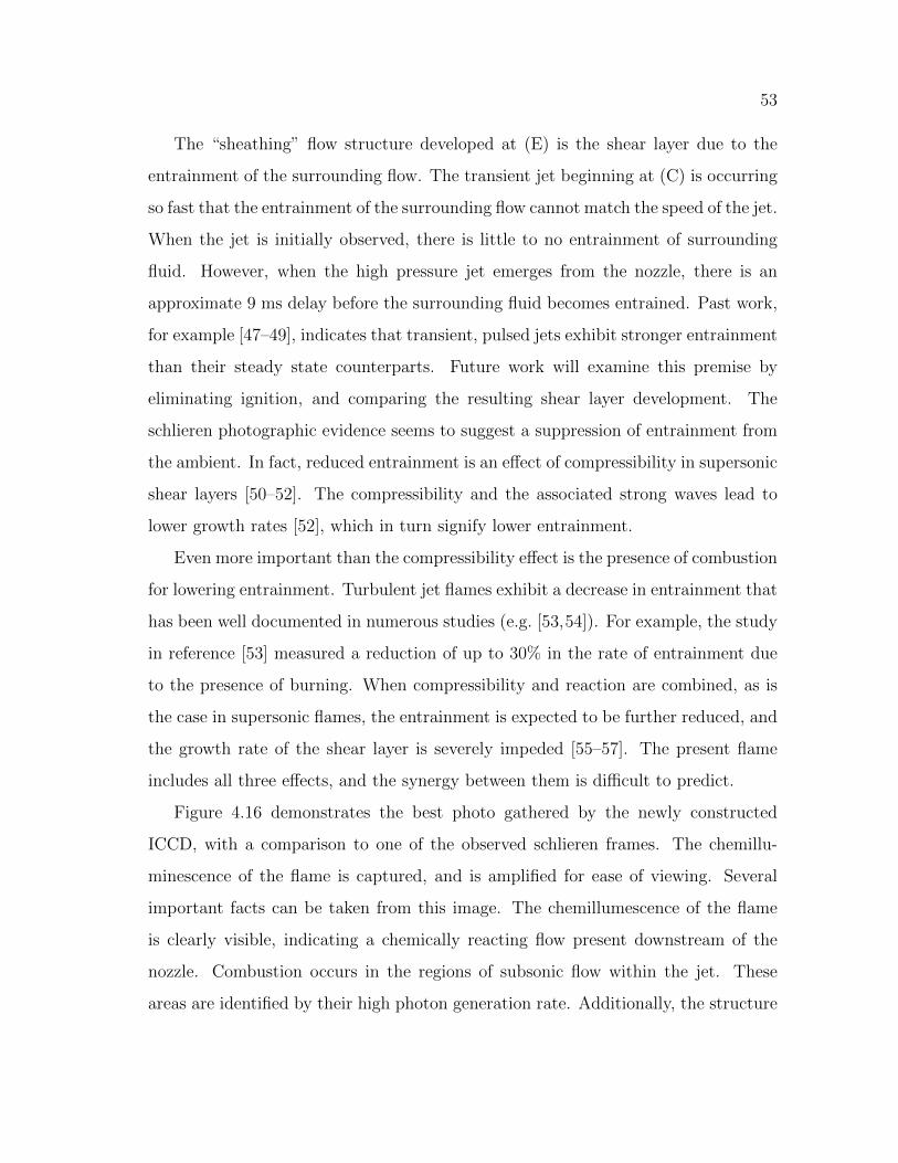
53

The “sheathing” flow structure developed at (E) is the shear layer due to the

entrainment of the surrounding flow. The transient jet beginning at (C) is occurring

so fast that the entrainment of the surrounding flow cannot match the speed of the jet.

When the jet is initially observed, there is little to no entrainment of surrounding

fluid. However, when the high pressure jet emerges from the nozzle, there is an

approximate 9 ms delay before the surrounding fluid becomes entrained. Past work,

for example [47–49], indicates that transient, pulsed jets exhibit stronger entrainment

than their steady state counterparts. Future work will examine this premise by

eliminating ignition, and comparing the resulting shear layer development. The

schlieren photographic evidence seems to suggest a suppression of entrainment from

the ambient. In fact, reduced entrainment is an effect of compressibility in supersonic

shear layers [50–52]. The compressibility and the associated strong waves lead to

lower growth rates [52], which in turn signify lower entrainment.

Even more important than the compressibility effect is the presence of combustion

for lowering entrainment. Turbulent jet flames exhibit a decrease in entrainment that

has been well documented in numerous studies (e.g. [53,54]). For example, the study

in reference [53] measured a reduction of up to 30% in the rate of entrainment due

to the presence of burning. When compressibility and reaction are combined, as is

the case in supersonic flames, the entrainment is expected to be further reduced, and

the growth rate of the shear layer is severely impeded [55–57]. The present flame

includes all three effects, and the synergy between them is difficult to predict.

Figure 4.16 demonstrates the best photo gathered by the newly constructed

ICCD, with a comparison to one of the observed schlieren frames. The chemillu-

minescence of the flame is captured, and is amplified for ease of viewing. Several

important facts can be taken from this image. The chemillumescence of the flame

is clearly visible, indicating a chemically reacting flow present downstream of the

nozzle. Combustion occurs in the regions of subsonic flow within the jet. These

areas are identified by their high photon generation rate. Additionally, the structure

54

Fig. 4.16. Ideal intensified image of transient flame. Backgroundnoises are minimized, causing flow structure and chemiluminescenceto be more easily observed. A direct comparison can be made betweenthe length scales of the schlieren and intensified images.

of the jet is comparable to the gathered schlieren images. Although solid boundaries

cannot be seen, the bright areas are comparable to the diamond patterns in Figure

4.15.

The ICCD was capable of determining the flame emergence from the nozzle.

While the schlieren setup would only give information regarding the overall density

gradients of the flow, chemiluminescence of the flame can be observed with the

ICCD. This means that even if there is a supersonic shock wave structure, it may

not necessarily be a flame. Because the ICCD is a triggered (gated) system, it can be

used to identify the flame emergence, and track its progress in space. This was useful

in comparing the model results to the experiment, as relations between distance and

time in Section 4.2 were made based on the timescales observed in the experiment.

The transient flame itself suffers from reproducibility based on the initial conditions

in the combustor, and the timing variations of the mechanical components used in

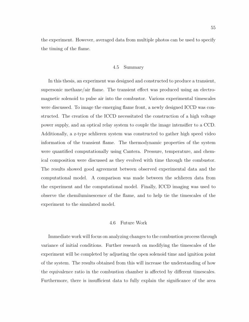
55

the experiment. However, averaged data from multiple photos can be used to specify

the timing of the flame.

4.5 Summary

In this thesis, an experiment was designed and constructed to produce a transient,

supersonic methane/air flame. The transient effect was produced using an electro-

magnetic solenoid to pulse air into the combustor. Various experimental timescales

were discussed. To image the emerging flame front, a newly designed ICCD was con-

structed. The creation of the ICCD necessitated the construction of a high voltage

power supply, and an optical relay system to couple the image intensifier to a CCD.

Additionally, a z-type schlieren system was constructed to gather high speed video

information of the transient flame. The thermodynamic properties of the system

were quantified computationally using Cantera. Pressure, temperature, and chem-

ical composition were discussed as they evolved with time through the combustor.

The results showed good agreement between observed experimental data and the

computational model. A comparison was made between the schlieren data from

the experiment and the computational model. Finally, ICCD imaging was used to

observe the chemiluminescence of the flame, and to help tie the timescales of the

experiment to the simulated model.

4.6 Future Work

Immediate work will focus on analyzing changes to the combustion process through

variance of initial conditions. Further research on modifying the timescales of the

experiment will be completed by adjusting the open solenoid time and ignition point

of the system. The results obtained from this will increase the understanding of how

the equivalence ratio in the combustion chamber is affected by different timescales.

Furthermore, there is insufficient data to fully explain the significance of the area

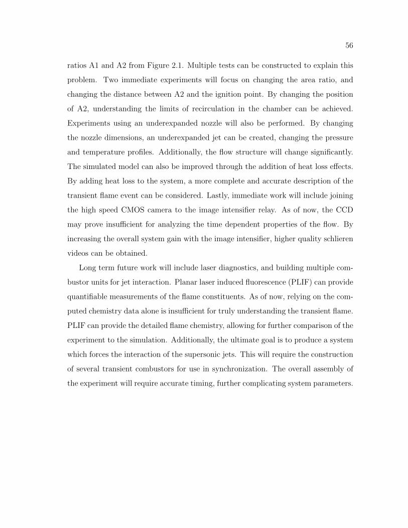
56

ratios A1 and A2 from Figure 2.1. Multiple tests can be constructed to explain this

problem. Two immediate experiments will focus on changing the area ratio, and

changing the distance between A2 and the ignition point. By changing the position

of A2, understanding the limits of recirculation in the chamber can be achieved.

Experiments using an underexpanded nozzle will also be performed. By changing

the nozzle dimensions, an underexpanded jet can be created, changing the pressure

and temperature profiles. Additionally, the flow structure will change significantly.

The simulated model can also be improved through the addition of heat loss effects.

By adding heat loss to the system, a more complete and accurate description of the

transient flame event can be considered. Lastly, immediate work will include joining

the high speed CMOS camera to the image intensifier relay. As of now, the CCD

may prove insufficient for analyzing the time dependent properties of the flow. By

increasing the overall system gain with the image intensifier, higher quality schlieren

videos can be obtained.

Long term future work will include laser diagnostics, and building multiple com-

bustor units for jet interaction. Planar laser induced fluorescence (PLIF) can provide

quantifiable measurements of the flame constituents. As of now, relying on the com-

puted chemistry data alone is insufficient for truly understanding the transient flame.

PLIF can provide the detailed flame chemistry, allowing for further comparison of the

experiment to the simulation. Additionally, the ultimate goal is to produce a system

which forces the interaction of the supersonic jets. This will require the construction

of several transient combustors for use in synchronization. The overall assembly of

the experiment will require accurate timing, further complicating system parameters.

57

REFERENCES

[1] Fry, R., “A Century of Ramjet Propulsion Technology Evolution,” Journal ofPropulsion and Power , Vol. 20, No. 1, 2004, pp. 27–58.

[2] Anderson, J., Modern Compressible Flow , 3rd ed., McGraw-Hill, 1982, pp. 120–145.

[3] Kloesel, K. J., Ratnayake, N. A., and Clark, C. M., “A Technology Pathway forAirbreathing, Combined-Cycle, Horizontal Space Launch Through SR-71 BasedTrajectory Modeling,” 17th AIAA International Space Planes and HypersonicSystems and Technologies Conference, San Francisco, CA, AIAA Paper 2011-2229, Apr. 2011.

[4] Roy, G., Frolov, S., Borisov, A., and Netzer, D., “Pulse Detonation Propulsion:Challenges, Current Status, and Future Perspective,” Progress in Energy andCombustion Science, Vol. 30, May 2004, pp. 545–672.

[5] Yan, Y., Fan, W., Wang, K., Zhu, X., and Mu, Y., “Experimental Investigationson Pulse Detonation Rocket Engine with Various Injectors and Nozzles,” ActaAstronautica, Vol. 69, 2011, pp. 39–47.

[6] Milton, B. and Pianthong, K., “Pulsed, Supersonic Fuel Jets – A Review ofTheir Characteristics and Potential for Fuel Injection,” International Journal ofHeat and Fluid Flow , Vol. 26, 2005, pp. 656–671.

[7] Zakrzewski, S., Milton, B., Pianthong, K., and Behnia, M., “Supersonic LiquidFuel Jets Injected into Quiescent Air,” International Journal of Heat and FluidFlow , Vol. 25, 2004, pp. 833–840.

[8] Cutler, A., “High-Frequency Pulsed Combustion Actuator Experiments,” AIAAJournal , Vol. 49, No. 9, Sept. 2011.

[9] Giuliani, F., Lang, A., Gradl, K., Siebenhofer, P., and Fritzer, J., “Air FlowModulation for Refined Control of the Combustion Dynamics Using a NovelActuator,” Journal of Engineering for Gas Turbines and Power , Vol. 134, Feb.2012.

[10] Gilarranz, J., Traub, L., and Rediniotis, O., “A New Class of Synthetic Jet Ac-tuators – Part I: Design, Fabrication and Bench Top Characterization,” Journalof Fluids Engineering , Vol. 127, Mar. 2005, pp. 367–376.

[11] Lefebvre, A., Ibrahim, A., and Benson, N., “Factors Affecting Fresh MixtureEntrainment in Bluff-Body Stabilized Flames,” Combustion and Flame, Vol. 10,1966, pp. 231–239.

[12] Longwell, J., Frost, E., and Weiss, M., “Flame Stability in Bluff Body Re-circulation Zones,” Industrial & Engineering Chemistry , Vol. 45, No. 8, 1953,pp. 1629–1633.

58

[13] Edelman, R. and Harsha, P., “Laminar and Turbulent Gas Dynamics in Com-bustors - Current Status,” Progress in Energy and Combustion Science, Vol. 4,1978, pp. 1–62.

[14] Sutton, G. and Biblarz, O., Rocket Propulsion Elements , 8th ed., John Wiley& Sons, New Jersey, 2010, pp. 57–63.

[15] Hill, P. and Peterson, C., Mechanics and Thermodynamics of Propulsion, 2nded., Addison-Wesley Publishing Company, 1992.

[16] Ehn, A., Johansson, O., Bood, J., Arvidsson, A., Li, B., and Alden, M., “Fluo-rescence Lifetime Imaging in a Flame,” Proceedings of the Combustion Institute,Vol. 33, 2011, pp. 807–813.

[17] Dam, N., Rodenburg, M., Tolboom, R., Stoffels, G., Huisman-Kleinherenbrink,P., and ter Meulen, J., “Imaging of an Underexpanded Nozzle Flow by UV LaserRayleigh Scattering,” Experiments in Fluids , Vol. 24, 1998, pp. 93–101.

[18] Docquier, N., Belhalfaoui, S., Lacas, F., and Darabiha, N., “Experimentaland Numerical Study of Chemiluminescence in Methane/Air High-PressureFlames for Active Control Applications,” Proceedings of the Combustion In-stitute, Vol. 28, 2000, pp. 1765–1774.

[19] Ikeda, Y., Kojima, J., and Hashimoto, H., “Local Chemiluminescence Spec-tra Measurements in a High-Pressure Laminar Methane/Air Premixed Flame,”Proceedings of the Combustion Institute, Vol. 29, 2002, pp. 1495–1501.

[20] Katanoda, H., Miyazato, Y., Masuda, M., and Matsuo, K., “Pitot Pressures ofCorrectly-Expanded and Underexpanded Free Jets from Axisymmetric Super-sonic Nozzles,” Shock Waves , Vol. 10, 2000, pp. 95–101.

[21] Tabei, K., Shirai, H., and Takakusagi, F., “Density Measurements of Underex-panded Free Jets of Air from Circular and Square Nozzles by Means of Moire-Schlieren Method,” JSME International Journal , Vol. 35, No. 2, 1992.

[22] Tkacik, P., Keanini, R., Srivastava, N., and Tkacik, M., “Color Schlieren Imag-ing of High-Pressure Overexpanded Planar Nozzle Flow Using a Simple, Low-Cost Test Apparatus,” Journal of Visualization, Vol. 14, No. 1, 2011, pp. 11–14.

[23] Settles, G., Schlieren and Shadowgraph Techniques , Springer-Verlag, New York,2001.

[24] Nasuti, F. and Onofri, M., “Shock Structure in Separated Nozzle Flows,” ShockWaves , Vol. 19, 2009, pp. 229–237.

[25] Bayeh, A. and Karpetis, A., “Miniaturized Combustor for Methane-Air After-burner,” Journal of Propulsion and Power , Feb. 2012, Submitted.

[26] Texas A&M University, Aerospace Engineering, “Transient Flames,” Au-gust 2010, [http://www.youtube.com/watch?v=chxdYtRqTOM. Accessed08/25/10.]

[27] Glassman, I., Combustion, 4th ed., Academic Press, 2008, pp. 240–250.

59

[28] Van den Schoor, F., Hermanns, R., van Oijen, J., Verplaetsen, F., and de Goey,L., “Comparison and Evaluation of Methods for the Determination of Flamma-bility Limits, Applied to Methane/Hydrogen/Air Mixtures,” Journal of Haz-ardous Materials , Vol. 150, 2008, pp. 573–581.

[29] Favaloro, M., “Ablative Materials,” Kirk-Othmer Encyclopedia of ChemicalTechnology , 2000.

[30] Mishra, C. and Yoav, P., “Incompressible and Compressible Flows ThroughRectangular Microorifices Entrenched in Silicon Microchannels,” Journal of Mi-croelectromechanical Systems , Vol. 14, No. 5, Oct. 2005, pp. 1000–1012.

[31] Kee, R., Chemically Reacting Flow: Thoery and Practice, 1st ed., John Wiley& Sons, 2003, pp. 649–683.

[32] Goodwin, D., “An Open-Source, Extensible Software Suite for CVDProcess Simulation,” Proceedings of CVD XVI , 2003, pp. 155–162,[http://code.google.com/p/cantera/. Accessed 01/15/11.].

[33] Smith, G., Golden, D., Frenklach, M., Moriarty, N., Eiteneer, B., Golden-berg, C., Bowman, T., Hanson, R., Song, S., Gardiner, W., Lissianski, V.,and Qin, Z., “GRI-Mech Source,” [http://www.me.berkeley.edu/gri mech/. Ac-cessed 01/15/11.]

[34] van Rossum, G., “Python Programming Language - Official Website,”[http://www.python.org/. Accessed 01/15/11.]

[35] Bergthorson, J. and Dimotakis, P., “Premixed Laminar C1-C2 StagnationFlames: Experiments and Simulations with Detailed Thermochemistry Mod-els,” Proceedings of the Combustion Institute, Vol. 31, 2007, pp. 1139–1147.

[36] Odedra, A. and Malalasekera, W., “Eularian Particle Flamelet Modeling ofa Bluff-Body CH4/H2 Flame,” Combustion and Flame, Vol. 151, Aug. 2007,pp. 512–531.

[37] Hamamatsu Photonics, Iwata City, Japan, Image Intensifiers , Sept. 2009.

[38] Eckbreth, A., Laser Diagnostics for Combustion Temperature and Species , 2nded., Gordon and Breach Publishers, 1996.

[39] Navon, D., Semiconductor Microdevices and Materials , CBS College Publishing,1986, pp. 387–397.

[40] Longmire, M., “SBIG Software - CCDOPS,”[http://www.sbig.com/Software.html. Accessed 10/15/11.]

[41] Santa Barbara Instruments Group, Santa Barbara, California, CCD CameraOperating Manual for the Model ST-4x, ST-5, and ST-6 , Jan. 1996, Revision2A.

[42] Markerink, W., “Camera Mounts & Registers,”[http://www.markerink.org/WJM/HTML/mounts.htm. Accessed 11/15/11.]

60

[43] Hiller, B., Paul, P., and Hanson, R., “Image-Intensified Photodiaode Arrayas a Fluorescence Detector in CW-Laser Experiments,” Review of ScientificInstruments , Vol. 61, No. 7, July 1990, pp. 1808–1815.

[44] Welford, W., Useful Optics , 1st ed., The University of Chicago Press, 1991.

[45] Zare-Behtash, H., Kontis, K., Gongora-Orozco, N., and Takayama, K., “Com-pressible Vortex Loops: Effect of Nozzle Geometry,” International Journal ofHeat and Fluid Flow , Vol. 30, 2009, pp. 561–576.

[46] White, F., Viscous Fluid Flow , 3rd ed., McGraw-Hill, 2006.

[47] Platzer, M., Simmons, J., and Bremhorst, K., “Entrainment Characteristics ofUnsteady Subsonic Jets,” AIAA Journal , Vol. 16, No. 3, 1977, pp. 282–284.

[48] Bremhorst, K. and Harch, W., “The Mechanism of Jet Entrainment,” AIAAJournal , Vol. 16, No. 10, 1978, pp. 1104–1106.

[49] Vermeulen, P., Ramesh, V., and Yu, W., “Measurements of Entrainment byAcoustically Pulsed Axisymmetric Air Jets,” ASME Journal , Vol. 108, July1986, pp. 479–484.

[50] Papamoschou, D. and Roshko, A., “The Compressible Turbulent Shear Layer:An Experimental Study,” Journal of Fluid Mechanics , Vol. 197, 1988, pp. 453–477.

[51] Samimy, M., Reeder, M., and Elliott, G., “Compressibility Effects on LargeStructures in Free Shear Flows,” Physics of Fluids , Vol. 4, No. 6, 1992, pp. 1251–1258.

[52] Elliot, G. and Samimy, M., “Compressibility Effects in Free Shear Layers,”Physics of Fluids , Vol. 2, No. 7, July 1990, pp. 1231–1240.

[53] Ricou, F. and Spalding, D., “Measurements of Entrainment by AxisymmetricalTurbulent Jets,” Journal of Fluid Mechanics , Vol. 11, 1961, pp. 21–32.

[54] Tacina, K. and Dahm, W., “Effects of Heat Release on Turbulent Shear Flows.Part 1. A General Equivalence Principle for Non-Buoyant Flows and its Appli-cation to Turbulent Jet Flames,” Journal of Fluid Mechanics , Vol. 415, 2000,pp. 23–44.

[55] Huh, H. and Driscoll, J., “Shock-Wave-Enhancement of the Mixing and the Sta-bility Limits of Supersonic Hydrogen-Air Jet Flames,” Twenty-Sixth Symposium(International) on Combustion, 1996, pp. 2933–2939.

[56] Driscoll, J., Huh, H., Yoon, Y., and Donbar, J., “Measured Lengths of Super-sonic Hydrogen-Air Jet Flames – Compared to Subsonic Flame Lengths – andAnalysis,” Combustion and Flame, Vol. 107, 1996, pp. 176–186.

[57] Miller, M., Bowman, C., and Mungal, M., “An Experimental Investigation ofthe Effects of Compressibility on a Turbulent Reacting Mixing Layer,” Journalof Fluid Mechanics , Vol. 356, 1998, pp. 25–64.

1

A Theoretical and Numerical Study on a Shock Wave

Interacting with a 2-D Discontinuous Area Enlargement

Nomenclature

a = speed of sound, RT

A = duct area (duct height times unit depth)

A2/A1 = ratio of large duct height to small duct height, degree of area change

cP = specific heat at constant pressure

D = function of Mach Number only, defined by Eq. (5)

h = sensible enthalpy, cPT

M = flow Mach Number, u/a

MS = incident shock strength

MSS = secondary shock strength

MTS = transmitted shock strength

P = pressure

PR, QR = right and left Riemann invariants, respectively

R = gas constant for air

T = temperature

u = velocity (1D)

= specific heat ratio (air)

= density

I. Introduction

CRAMJETS have been extensively studied since the 1950’s due to the to highly complex nature of the flows,

short flow residency times, difficulties in mixing fuel and oxidizer in the combustion chamber, airframe

integration issues, and high heat transfer rates. One major drawback of scramjet engines is the need to accelerate the

vehicle to supersonic velocities to provide the scramjet inlet with a sufficient amount of high-kinetic energy air. To

overcome this difficulty, two major approaches have been developed, with many more still under research. Usually,

a second engine is employed to accelerate the vehicle: if this is done with a rocket, it is called a Rocket-Based

Combined Cycle (RBCC) system; if done with a turbine engine, a Turbine-Based Combined Cycle (TBCC) system.

However, carrying two entire propulsion systems onboard for the entire flight results in increases in the vehicle size

and weight, increases in the complexity and number of failure points, a reduction of the payload capacity, and

ultimately increases in the vehicle cost.

One approach to accelerating the scramjet is the transient inlet concept (TIC) shown in Fig. 1. In this method, a

scramjet inlet is outfitted with small injector ducts that inject either shock or detonation waves into the main engine

flowpath. Executed in a rapidly pulsing manner similar to that of a Pulsed Detonation Engine (PDE), these waves

serve to accelerate the flow behind them, potentially inducing flow into the engine inlet. However, there are many

scientific and technical challenges associated with assessing the feasibility of this concept, such as unsteady shock

wave motion in ducts, shock-shock interactions, shock-induced free shear layers, mixing enhancement, and many

S

Figure 1. Motivation concept. Transient Inlet Concept was conceived by R. Bowersox and R. Jeffries (AFOSR)

2

more (see Fig. 1). This study will address the first: unsteady shock wave motion in ducts.

II. Background

Unsteady shock wave motion through ducts has been extensively studied due to the wide variety of potential

applications, such as hazardous explosions in underground tunnels, gas transmission pipes, exhaust systems of

internal combustion engines and blast shelter design. These complicated flow fields are rich in a large variety of

fundamental fluid dynamic phenomena, i.e. shock wave reflections, shock-shock interactions, shock-vortex

interactions, etc. Combined with the relatively simple geometries, these flows are excellent testbeds for improving

our understanding of fluid dynamics.

Historically, these studies fall into several categories: shock waves in turning ducts(1-6)

, shock waves turning

corners(7-11)

, shock waves in branching ducts(12-17)

, shock waves in ducts with baffles/obstacles(18-26)

, shock wave

focusing(27-34)

, and shock waves in ducts of varying cross-sections (the present paper will only consider changes in

geometry). An excellent comprehensive review of these topics can be found in Ref. 35. Since the original works

done by Chester36,37

, Chisnell38

, and Whitham39-41

, shock wave motion through ducts of varying cross-sectional area

has been treated by numerous researchers. A few studies(42-48)

treat a wide variety of geometry changes both

mathematically and experimentally, including curved and straight ducts, “stairways”, and even airfoils. Some(49,50)

specialize in area changes that converge then diverge, akin to nozzle flows. These geometries can be classified

according to two features: continuous (smooth, gradual) or discontinuous (sudden, abrupt), and an area enlargement

or area reduction.

Much of the past work has focused on continuous area changes, since there are several theoretical methods

(Chester-Chisnell-Whitham theory36-41

, Skews theory8, shock dynamics ray-shock theory

51, Rudinger’s theory

52,

Method of Characteristics) available to analyze them and several quasi-1D numerical methods (Second-order

Hydrodynamic Automatic Mesh Refinement Code53

, Generalized Riemann Problem codes54

, Random Choice

Method codes55

) available to solve them. These geometries usually involve a gradual area change manifested by an

area change segment characterized by its length to height ratio. Generally speaking, the smaller the divergence

angle and the longer the area change segment, the closer the experimental and numerical results are to the theoretical

results. Several studies have examined unsteady shock waves interacting with both continuous area enlargements

and reductions(55,56)

, only area enlargements(57,58)

, and only area reductions(59-62)

. In particular, pseudo-steady and

unsteady shock wave reflections from a smoothly converging (inclined) wall have received much attention. For a

recent comprehensive report of the work done on these flows, see Ref. 63.

This report focuses on discontinuous area changes because these are the types of interactions seen in the transient

inlet concept. The past work in this subfield covers both discontinuous area enlargements and reductions(64,65)

, only

area reductions(66-69)

, and area enlargements. In the case of discontinuous area reductions, there exists a bifurcation

in the potential flow patterns, where one of three possibilities exists. Thus, the studies in this area focus on

analyzing this peculiarity. However, this does not exist for discontinuous area enlargements, where the flow pattern

is deterministic. These flows can be further sorted according to the number of degrees of freedom of the geometry:

axisymmetric (cylindrical) and rectangular. There are a few studies that consider both axisymmetric and rectangular

discontinuous area enlargements70-73

. Axisymmetric geometries are prevalent in the literature(74-79)

, since the easiest

case is the shock wave exiting the open end of a shock tube(80-84)

. These flows usually have a spherically expanding

shock wave followed by a vortex ring. Since scramjet ducts are often rectangular, this study considers an

asymmetric rectangular geometry (backwards-facing step). As such, the most relevant works are those regarding

discontinuous rectangular area enlargements, such as those found in Ref. 85-98. These include geometries ranging

from true backwards-facing steps to expansion chambers, open square-shaped and diamond-shaped ends of shock

0.1 0.2 0.3 0.4 0.5 0.6 0.7 0.8 0.9 11

1.5

2

2.5

3

3.5

4

Area Ratio (A1/A

2)

Incid

en

t S

ho

ck S

tre

ng

th (

Ms)

Figure 2. Existing body of work shown in parameter space.

3

tubes, and adjoining square cavities. These works qualitatively and quantitatively comment on the diffracting shock

shape, corner vortex location, shock-vortex interactions, and secondary shock structures. [WILL ELABORATE

MORE HERE] However, the majority of these studies are numerical and experimental, with very limited theoretical

treatment of these flows. Second, additional flow features are illuminated in this work that were not covered

previously. Third, the cases studied thus far are sporadic and spot the parameter space; whereas this is the first true

parametric study of these flows. This paper will compare theoretical and numerical results, and identify the time-

accurate primary and secondary flow structures present in these flows.

III. Methodology

All of the simulations and calculations performed herein assume inviscid compressible flows in air. The range

of incident shock strengths studied was 1 < MS < 3 over area ratios 1.1 A2/A1 2.0. Limiting the incident shock

strength to these values covers all possible wave diagrams for these flows while simplifying the gas dynamics. At

the upper limit (MS = 3), the temperature behind the incident shock (~800K) is not sufficient to cause noticeable real

gas effects, such as ioization, dissociation, or chemical reactions. Thus, for these studies the thermally perfect

equation of state will be used (as well as the calorically perfect equation of state). In addition, since the appropriate

time scales (~1ms) are too short for a significant amount of heat transfer, the flows are reasonably assumed to be

adiabatic and non-conducting. The range of area ratios was chosen to provide scenarios that would range from only

a small perturbation from theory up to a matching of channel heights between the main engine duct and the shock

injector duct.

A. Theoretical In addition to the above assumptions, the theoretical treatment of the problem also assumes a “steady state”.

Though the primary difficulty of this problem is its transient nature, if one were to wait a sufficiently long enough

time such that all transient phenomena due to the area change interaction were to subside and all major wave

strengths were no longer being modified, then the wave system could be said to have approached a “steady state”.

This also means that the primary waves (shocks, expansions) travel with a constant velocity in an inviscid flow and

uniform flow regions separate the primary waves. Furthermore, the theory will assume quasi-1D flow, which is

consistent with modern approaches to these problems. Following the algorithm presented in Rudinger 195552

, these

assumptions simplify the Euler equations to:

Conservation of Mass (COM):

L L L R R Ru A u A (1)

Conservation of Energy (COE):

2 2

1 21 2 0

2 2

u uh h h (2)

Both conservation laws hold across the area change, assuming the flow expands isentropically through the area

change (i.e. no flow separation or standing shocks). Subscripts L and R denote the left and right sides of the area

change respectively. By substituting the isentropic definition of the stagnation enthalpy combined with COE (Eq.

(2))

2 1/( 1)0 1

(1 )2

L

L

M

(3)

Into Eq. (1) for both L and R (and similarly for TL and TR), and using the definitions of the Mach Number and

sound speed, one obtains an isentropic statement of COM as a function only of M, that is 2 1

A / A ( , )L R

f M M

4

1

2( 1)2

1 2

2

1

1 2( 1)2

2 1

11

2

11

2

M MA

A

M M

(4)

Which can be rewritten as ALDL = ARDR, where

1

2( 1)21

12

MD

M

(5)

This function of Mach Number only has two branches: a subsonic branch where D increases with increasing M

up to a maximum, and a supersonic branch where D decreases with increasing M. Now manipulate COE (Eq. (2))

by substituting in the definitions of cP and a, which yields

2 2 2 2

1 1 2 2

1 2 1 2

a u a u

(6)

Or

2 2 2 2

1 1 2 2

1 11 1

2 2a M a M

(7)

Eqs. (6) and (7) along with Eq. (4) are the forms of the conservation laws that will be used in this algorithm.

Finally, since centered expansion waves are present, the opposite Riemann invariants hold across them:

For left-running (Q) waves

2

1R

aP u const

(8)

For right-running (P) waves

2

1R

aQ u const

(9)

Now that a useful form of the conservation laws has been obtained, one can apply these governing equations to

the problem at hand. Rudinger 195552

presents five possible wave patterns that could be seen in the given parameter

space (MS, A2/A1), illustrated in Fig. 3 below (cases 1-5). It was later discovered that a sixth possible case exists,

shown in Fig. 3. From this analysis, three primary waves appear: the transmitted shock that propagates into the

large duct, an expansion reflected upstream into the small duct, and a secondary left-facing shock wave somewhere

in the large duct.

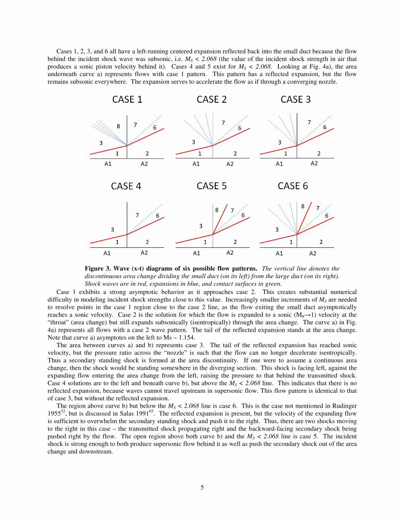
5

Cases 1, 2, 3, and 6 all have a left-running centered expansion reflected back into the small duct because the flow

behind the incident shock wave was subsonic, i.e. MS < 2.068 (the value of the incident shock strength in air that

produces a sonic piston velocity behind it). Cases 4 and 5 exist for MS < 2.068. Looking at Fig. 4a), the area

underneath curve a) represents flows with case 1 pattern. This pattern has a reflected expansion, but the flow

remains subsonic everywhere. The expansion serves to accelerate the flow as if through a converging nozzle.

Case 1 exhibits a strong asymptotic behavior as it approaches case 2. This creates substantial numerical

difficulty in modeling incident shock strengths close to this value. Increasingly smaller increments of MS are needed

to resolve points in the case 1 region close to the case 2 line, as the flow exiting the small duct asymptotically

reaches a sonic velocity. Case 2 is the solution for which the flow is expanded to a sonic (M81) velocity at the

“throat” (area change) but still expands subsonically (isentropically) through the area change. The curve a) in Fig.

4a) represents all flows with a case 2 wave pattern. The tail of the reflected expansion stands at the area change.

Note that curve a) asymptotes on the left to Ms ~ 1.154.

The area between curves a) and b) represents case 3. The tail of the reflected expansion has reached sonic

velocity, but the pressure ratio across the “nozzle” is such that the flow can no longer decelerate isentropically.

Thus a secondary standing shock is formed at the area discontinuity. If one were to assume a continuous area

change, then the shock would be standing somewhere in the diverging section. This shock is facing left, against the

expanding flow entering the area change from the left, raising the pressure to that behind the transmitted shock.

Case 4 solutions are to the left and beneath curve b), but above the MS < 2.068 line. This indicates that there is no

reflected expansion, because waves cannot travel upstream in supersonic flow. This flow pattern is identical to that

of case 3, but without the reflected expansion.

The region above curve b) but below the MS < 2.068 line is case 6. This is the case not mentioned in Rudinger

195552

, but is discussed in Salas 199165

. The reflected expansion is present, but the velocity of the expanding flow

is sufficient to overwhelm the secondary standing shock and push it to the right. Thus, there are two shocks moving

to the right in this case – the transmitted shock propagating right and the backward-facing secondary shock being

pushed right by the flow. The open region above both curve b) and the MS < 2.068 line is case 5. The incident

shock is strong enough to both produce supersonic flow behind it as well as push the secondary shock out of the area

change and downstream.

Figure 3. Wave (x-t) diagrams of six possible flow patterns. The vertical line denotes the

discontinuous area change dividing the small duct (on its left) from the large duct (on its right).

Shock waves are in red, expansions in blue, and contact surfaces in green.

6

Knowing the conservation laws and the wave patterns, a computer code was developed to solve these flow

fields. All algorithms involved guessing on a flow variable, proceeding with calculations over the entire flow field,

and matching both the pressure and velocity across the transmitted shock (which must always exist). If the two do

not yield the same strength of the transmitted shock, the guess is updated via a simple bisection method until the

solution converges (usually to a tolerance of 0.001 on velocity). The solution usually converged in 12 iterations or

less. Some useful notes on the algorithms used:

• For each case, the flow variable iterated on was: case 1 – the sound speed following the reflected

expansion (a8), case 2 – the incident shock strength (MS), cases 3-6 – the transmitted shock strength

(MTS).

• When using COM (Eq. (4)) across the area change, one must always go from the smaller duct to the

larger duct. Otherwise, the value for D (see Eq. (5)) will exceed its maximum value, and the solution will

not be found.

• Use moving normal shock jump conditions across both the incident and transmitted shocks.

• Total enthalpy is not conserved (across all moving waves), except across the area change (when a standing

shock is not present).

• When jumping across a rarefaction wave, use the isentropic relations to find the pressures, not COE.

• The algorithm for the cases with a stationary shock (3 and 4) is taken from Modern Compressible Flow99

(example 5.7). Note that this portion does not use Eq. (4).

• The secondary moving shock in cases 5 and 6 is a left-facing shock wave, but it is pushed right by the

expanded flow (due to the area change). The calculations find the velocity with which the shock is

moving to the left using a temporary change in reference frame.

The theoretical algorithm is not physically limited to this parameter space; however, the foundational theory

breaks down above MS ~ 4, producing inaccurate results. The algorithm also works for any area ratio (A2/A1 > 1),

but rather the scope of this report is the limiting factor.

B. Theoretical Verification In order to deem the theoretical results produced by this solution algorithm as reliable, the code must be verified

against the literature. Salas 199165

analyzed discontinuous area enlargements and area contractions, focusing on a

bifurcation in the latter. They used a similar inviscid “steady state” algorithm and provided selected results for each

case, as well as a detailed mapping of the cases to the parameter space.

The comparison between their results and the current results for the Mach Number in various flow regions for the

selected cases are tabulated below:

Table 1. Comparison between Salas 199165

And Current Results for Selected Cases.

Case A2/A1 Ms M3 M8 M7 M6

1 0.5 (2) 1.1 0.154 0.222 0.109 0.109

0.15416 0.22205 0.10857 0.10858

2 0.5 (2) 1.303 0.409 - 0.306 0.307

0.40851 - 0.3059 0.30645

3 0.5 (2) 1.5 0.609 - 0.427 0.447

0.60429 - 0.42656 0.44688

6 0.5 (2) 1.85 0.871 2.197 0.65 0.698

0.87117 2.1972 0.6502 0.69861

5 0.5 (2) 2.5 1.197 2.23 0.994 1.058

1.197 2.23 0.99379 1.0579

For each case, the top row is their results and the second row is the results produced here. They did not show

results for case 4. The majority of the error is due to the rounding to the third decimal place in Salas 199165

,

therefore it can be stated that our results match to three decimal places. None of the errors exceed 1%.

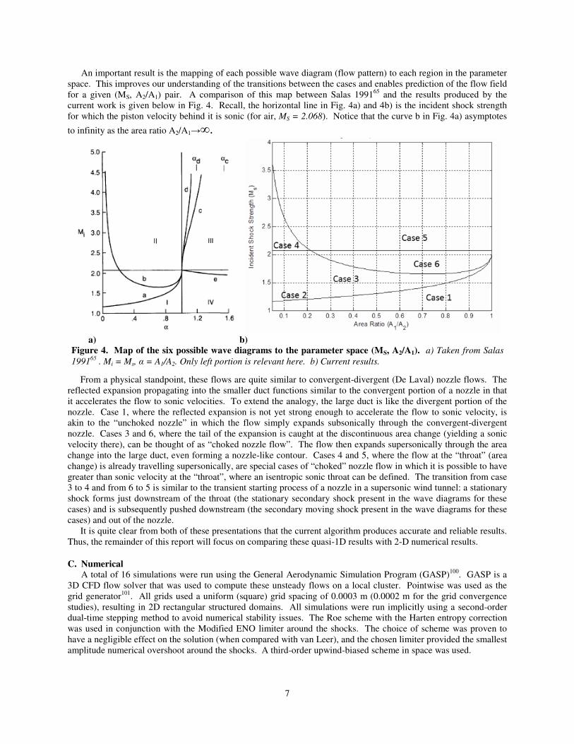
7

An important result is the mapping of each possible wave diagram (flow pattern) to each region in the parameter

space. This improves our understanding of the transitions between the cases and enables prediction of the flow field

for a given (MS, A2/A1) pair. A comparison of this map between Salas 199165

and the results produced by the

current work is given below in Fig. 4. Recall, the horizontal line in Fig. 4a) and 4b) is the incident shock strength

for which the piston velocity behind it is sonic (for air, MS = 2.068). Notice that the curve b in Fig. 4a) asymptotes

to infinity as the area ratio A2/A1.

From a physical standpoint, these flows are quite similar to convergent-divergent (De Laval) nozzle flows. The

reflected expansion propagating into the smaller duct functions similar to the convergent portion of a nozzle in that

it accelerates the flow to sonic velocities. To extend the analogy, the large duct is like the divergent portion of the

nozzle. Case 1, where the reflected expansion is not yet strong enough to accelerate the flow to sonic velocity, is

akin to the “unchoked nozzle” in which the flow simply expands subsonically through the convergent-divergent

nozzle. Cases 3 and 6, where the tail of the expansion is caught at the discontinuous area change (yielding a sonic

velocity there), can be thought of as “choked nozzle flow”. The flow then expands supersonically through the area

change into the large duct, even forming a nozzle-like contour. Cases 4 and 5, where the flow at the “throat” (area

change) is already travelling supersonically, are special cases of “choked” nozzle flow in which it is possible to have

greater than sonic velocity at the “throat”, where an isentropic sonic throat can be defined. The transition from case

3 to 4 and from 6 to 5 is similar to the transient starting process of a nozzle in a supersonic wind tunnel: a stationary

shock forms just downstream of the throat (the stationary secondary shock present in the wave diagrams for these

cases) and is subsequently pushed downstream (the secondary moving shock present in the wave diagrams for these

cases) and out of the nozzle.

It is quite clear from both of these presentations that the current algorithm produces accurate and reliable results.

Thus, the remainder of this report will focus on comparing these quasi-1D results with 2-D numerical results.

C. Numerical

A total of 16 simulations were run using the General Aerodynamic Simulation Program (GASP)100

. GASP is a

3D CFD flow solver that was used to compute these unsteady flows on a local cluster. Pointwise was used as the

grid generator101

. All grids used a uniform (square) grid spacing of 0.0003 m (0.0002 m for the grid convergence

studies), resulting in 2D rectangular structured domains. All simulations were run implicitly using a second-order

dual-time stepping method to avoid numerical stability issues. The Roe scheme with the Harten entropy correction

was used in conjunction with the Modified ENO limiter around the shocks. The choice of scheme was proven to

have a negligible effect on the solution (when compared with van Leer), and the chosen limiter provided the smallest

amplitude numerical overshoot around the shocks. A third-order upwind-biased scheme in space was used.

a) b)

Figure 4. Map of the six possible wave diagrams to the parameter space (MS, A2/A1). a) Taken from Salas

199165

. Mi = Ms, = A1/A2. Only left portion is relevant here. b) Current results.

8

The simulations were chosen to study three area ratios at four incident shock strengths each. The incident shock

strength determined the case (discussed above). After these initial twelve simulations were run for 2500 time steps

each, more information was desired from those with the more complicated flow fields. Hence four cases were run

for double the amount of time (5000 time steps each) and with a larger domain (0.7 m in length). Thus, 16

simulations were run and discussed. The domains for all three geometries are shown below (see Fig. 5), and a

summary of the remaining numerical settings can be found in the Appendix.

The first 0.05m of the small duct (to the left of the dashed line) was initialized to the post-shock conditions

appropriate for the case, and the remaining 0.05m of the small duct and the entire large duct were initialized to the

reference conditions. All boundaries were walls except for the leftmost (inflow) and rightmost (outflow)

boundaries, and the area ratio was changed via moving the top wall of the large duct.

D. Grid Covergence Studies

To ensure that the result were independent of the chosen grid, grid convergence studies were performed for all

16 simulations. These simulations were run using a uniform square grid spacing of 0.0002m, and the same time step

and total run time as the previous simulations. At each time step, the difference in pressures between the two grids

was calculated at each grid point along a single i-line in the domain. The average difference (error) between the two

grids was calculated for each time step, and these values were subsequently averaged for each simulation. For the

initial 12 cases, the average error was < 1%, and for the four long cases, < 4%. It was noticed that the largest errors

tended to be differences in amplitudes (numerical overshoots) at shock locations, but both grids placed the shocks in

the same locations. To quantify this, the difference in the transmitted shock location was compared for the two

grids, averaged over the total simulation time for each case. This matched to within 0.25% for the first 12 cases, and

to within 0.125% for the four long cases. The error in the transmitted shock location decreased over time (see Fig.

6). It can be safely declared that these studies are grid independent.

E. Numerical Verification and Validation To further verify that the chosen methods and settings produce accurate results, the same numerical methods

were applied to several studies from the literature. Selection criteria included a discontinuous area enlargement with

a rectangular cross-section, preferably with comparisons of

experimental and numerical results. The author was only able to

find three sources that matched these criteria, of which two are

presented here.

Shock Wave Interacting with a Square Cavity:

Figure 5. Domain Geometry for Simulations (all dimensions in meters)

0 0.1 0.2 0.3 0.4 0.5 0.6 0.7 0.8 0.9 1

x 10-3

0

0.1

0.2

0.3

0.4

0.5

0.6

0.7

0.8

0.9

Time (sec)

% E

rror

in T

ransm

itte

d S

hock L

ocatio

n

Figure 6. % Error in the transmitted shock location over time for case (1.50, 2.0). Note:

All case nomenclature defined as (MS, A2/A1).

9

Igra et al. (1996)88

did an experimental and numerical study of a shock wave interacting with a square cavity at

two different incident shock strengths, MS = 1.30 and MS = 2.032. The first part of the simulations before the shock

wave interacts with the opposing cavity face are comparable here. In Fig. 7, the MS = 2.032 case is shown for several

isntants in time. The time step was not given in Igra et al. 199688

, but was chosen here as 6.25E-7 sec. The initial

conditions are P0 = 0.9 bar and T0 = 22.6°C, and the uniform grid size was ~ 0.0002m (or 0.2 mm). The results

show excellent agreement, capturing all of the flow features. The minute differences are due to errors in the shock

starting location and in specific data visualization techniques (number and spacing of density contours). The

agreement with the previous numerical simulation serves to verify our numerical methods, and the agreement with

experiment validates the chosen models.

Shock Wave Interacting with an Expansion Chamber:

Igra et al. (2001)90

also performed an experimental and theoretical study of a shock wave interacting with

double-bend ducts that included an extension of the middle leg (i.e. an expansion chamber). They studied four

geometries, only two of which will be compared below. One had a shorter expansion chamber of length 80 mm, and

the second had a larger expansion chamber of length 160 mm (see Fig. 8). The long expansion chamber was studied

at an incident shock strength of MS = 1.53 with ambient conditions: P0 = 0.982 bar and T0 = 23.7°C. The time step

was chosen here (not reported in Ref. 90) to be t = 1e-06 sec. Again, the observed agreement verified and

validated our methods.

a) b) c)

Figure 7. Shock Wave Interacting with a Square Cavity at MS = 2.032. Experimental schlieren/shadowgraphs taken from Igra et al. 1996

88. b)

Numerical isopynics taken from Igra et al. 199688

c) Numerical isopycnics

produced from current numerical methods.

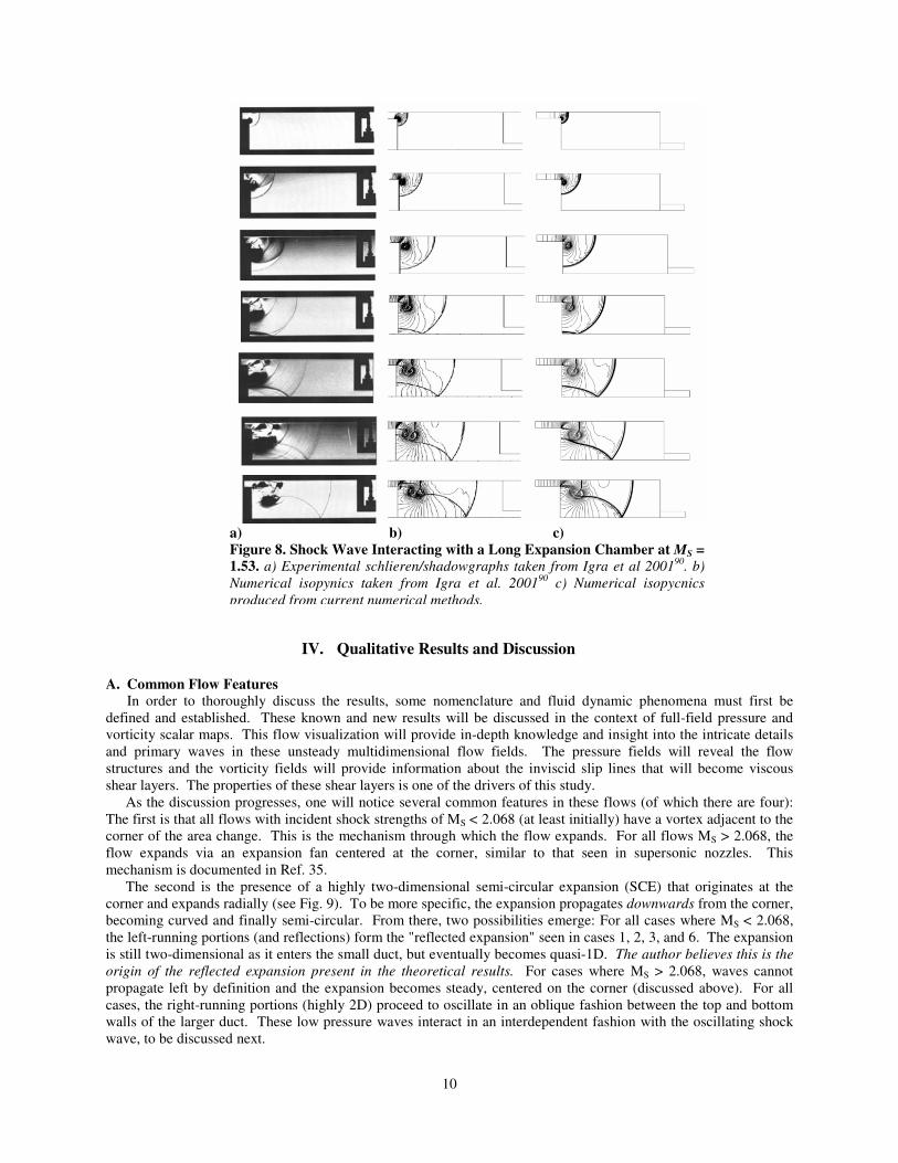
10

IV. Qualitative Results and Discussion

A. Common Flow Features In order to thoroughly discuss the results, some nomenclature and fluid dynamic phenomena must first be

defined and established. These known and new results will be discussed in the context of full-field pressure and

vorticity scalar maps. This flow visualization will provide in-depth knowledge and insight into the intricate details

and primary waves in these unsteady multidimensional flow fields. The pressure fields will reveal the flow

structures and the vorticity fields will provide information about the inviscid slip lines that will become viscous

shear layers. The properties of these shear layers is one of the drivers of this study.

As the discussion progresses, one will notice several common features in these flows (of which there are four):

The first is that all flows with incident shock strengths of MS < 2.068 (at least initially) have a vortex adjacent to the

corner of the area change. This is the mechanism through which the flow expands. For all flows MS > 2.068, the

flow expands via an expansion fan centered at the corner, similar to that seen in supersonic nozzles. This

mechanism is documented in Ref. 35.

The second is the presence of a highly two-dimensional semi-circular expansion (SCE) that originates at the

corner and expands radially (see Fig. 9). To be more specific, the expansion propagates downwards from the corner,

becoming curved and finally semi-circular. From there, two possibilities emerge: For all cases where MS < 2.068,

the left-running portions (and reflections) form the "reflected expansion" seen in cases 1, 2, 3, and 6. The expansion

is still two-dimensional as it enters the small duct, but eventually becomes quasi-1D. The author believes this is the

origin of the reflected expansion present in the theoretical results. For cases where MS > 2.068, waves cannot

propagate left by definition and the expansion becomes steady, centered on the corner (discussed above). For all

cases, the right-running portions (highly 2D) proceed to oscillate in an oblique fashion between the top and bottom

walls of the larger duct. These low pressure waves interact in an interdependent fashion with the oscillating shock

wave, to be discussed next.

a) b) c)

Figure 8. Shock Wave Interacting with a Long Expansion Chamber at MS = 1.53. a) Experimental schlieren/shadowgraphs taken from Igra et al 2001

90. b)

Numerical isopynics taken from Igra et al. 200190

c) Numerical isopycnics

produced from current numerical methods.

11

The third is the presence of a shock (or compression) wave, hereafter termed the Oscillating Shock Wave

(OSW). As the transmitted shock propagates through the area change, the top portion curves upwards to meet the

duct top wall. As the curvature expands and the wall shock travels up the upper left wall, it eventually reaches the

top wall and reflects off of it. Jiang et al 199776

term this reflected wave the "reflected shock wave". This wave

passes (on its downward journey) through the corner vortex, interacting with it. The surviving portion continues to

propagate downwards and reflect off of the bottom wall. After this (second) reflection, it continues to bounce

between the top and bottom walls, giving it the name the oscillating shock wave. With each reflection, it sends

oblique compressions or shock waves (depending on the gradients) both to the left and right, establishing other

prominent flow features. The right-running oblique compressions travel faster than the transmitted shock, and thus

eventually catch up to and merge with it. Each time this happens, the transmitted shock experiences a sudden jump

in its strength. Each new reflection also brings a decay in the strength of the OSW, such that over a sufficient

amount of time the OSW becomes indistinguishable. This shock has very interesting acoustic properties since it

behaves like a plucked guitar string. The primary difference is that its length is a function of time, since the

transmitted shock (corresponding to its right end) continues to propagate right, and its left endpoint also moves

(though in a significantly less predictable manner). The frequency of its oscillations determines how often oblique

shocks or compressions are sent upstream and downstream, and thus in turn, how often and to what degree the

transmitted shock strength is modified. The oscillating shock wave has been seen by other researchers, where it is

inidicated by the red arrows in Fig. 10. An example of the oscillating shock wave in the current results is given

below in Fig. 11.

The interplay between the semi-circular expansion and the OSW is what drives the majority of the flow features

seen in these flows (see Fig. 13). The degree of the area change affects this interaction: Since the SCE initially

propagates downwards and the shock wave initially propagates upwards, the degree of area change essentially

controls the “phase difference” between the two waves. The smaller the area change, the more closely the OSW

follows the SCE, and thus the smaller the phase difference. The larger the area change, the further apart the two

Figure 9. Full-Field Pressure Map for Case (1.30, 1.5), illustrating the semi-circular expansion and the formation

of the reflected expansion.

12

waves are in time and space, and thus the larger the phase difference. In fact, at an area ratio of 2, the waves are

initially nearly opposite, i.e. the phase difference is approximately 180°. This can be seen in Fig. 13c), where the

wall shock reaches the duct top wall and the leading wave of the SCE reaches the duct bottom wall at almost the

same instant. However, both waves decay over time, and this leads to a time variance of the phase difference due to

transient changes in the amplitude and period of both waves.

Figure 10. Examples of Oscillating Shock Wave. Red arrows indicate presence of OSW. All photos

taken from Handbook of Shock Waves35

.

Figure 11. Example of oscillating shock wave. Case (2.48, 1.1)

Figure 12. Illustration of phase difference between SCE and OSW. a) Case (1.93, 1.1)

b) Case (1.93, 1.5) c) Case (1.85, 2.0)

13

The fourth is the presence of the transmitted shock. It must be there, since it is the continuation of the incident

shock through the area change. A triple point propagates along its surface that provides an interface between low

and high pressure regions behind the transmitted shock. The low pressure region is most likely caused by the right-

running expansions (discussed above) that oscillate between the top and bottom walls, and it also causes a bulging

(or curving) of the transmitted shock. The lower the pressure, the more the transmitted shock curves. The high

pressure region is caused by the attachment of the oblique shocks (or compressions) generated by the OSW to the

transmitted shock. The triple point always moves into the low pressure region and leaves the high pressure region

behind it. The transmitted shock is straightened by the passage of the triple point and the creation of the high

pressure region. In other words, the low pressure region curves the transmitted shock and the high pressure region

straightens it. Over time, as the gradients between the two lessen, the curvature lessens, and each subsequent

passage of the triple point results in a straighter transmitted shock, until the transmitted shock finally becomes

planar.

Figure 13. Illustration of the interplay between the OSW and the SCE. Case (1.10, 2.0)

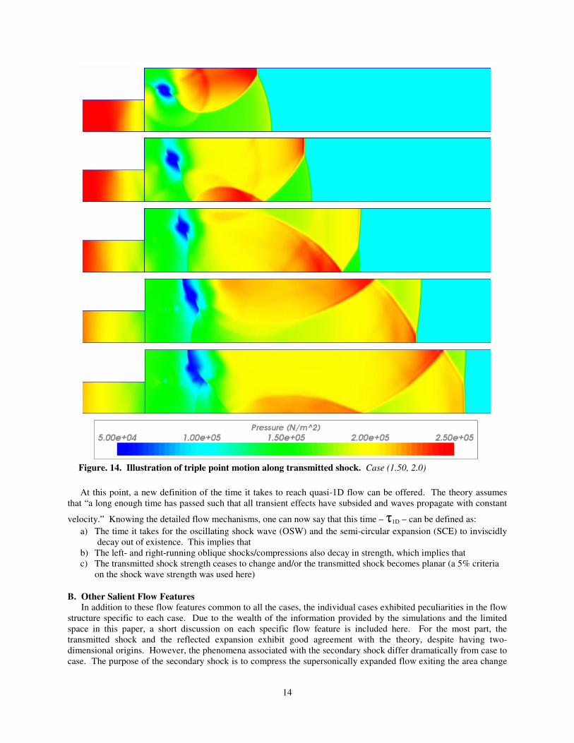
14

At this point, a new definition of the time it takes to reach quasi-1D flow can be offered. The theory assumes

that “a long enough time has passed such that all transient effects have subsided and waves propagate with constant

velocity.” Knowing the detailed flow mechanisms, one can now say that this time – 1D – can be defined as:

a) The time it takes for the oscillating shock wave (OSW) and the semi-circular expansion (SCE) to inviscidly

decay out of existence. This implies that

b) The left- and right-running oblique shocks/compressions also decay in strength, which implies that

c) The transmitted shock strength ceases to change and/or the transmitted shock becomes planar (a 5% criteria

on the shock wave strength was used here)

B. Other Salient Flow Features In addition to these flow features common to all the cases, the individual cases exhibited peculiarities in the flow

structure specific to each case. Due to the wealth of the information provided by the simulations and the limited

space in this paper, a short discussion on each specific flow feature is included here. For the most part, the

transmitted shock and the reflected expansion exhibit good agreement with the theory, despite having two-

dimensional origins. However, the phenomena associated with the secondary shock differ dramatically from case to

case. The purpose of the secondary shock is to compress the supersonically expanded flow exiting the area change

Figure. 14. Illustration of triple point motion along transmitted shock. Case (1.50, 2.0)

15

to the conditions behind the transmitted shock. The method through which the flow accomplishes this is a highly

complex, multidimensional, and transient process that requires significant further investigation.

For the cases with secondary shocks (3-6), the flow most commonly accomplishes the purpose of the secondary

shock through an oblique shock train. As mentioned before, these flows exhibit characteristics similar to nozzle

flows, and the oblique shock train established is quite reminiscent of the Mach diamond pattern found in nozzle

flows and scramjet isolators (should one mirror the flow about the bottom wall). These oblique

shocks/compressions occasionally form Mach stems that sometimes disappear over time. Likewise, the number of

oblique shocks/compressions in the train depends upon the case being studied. In all cases, the right-running

compressions caught up to and merged with the transmitted shock.

For all of the A2/A1 = 1.1 cases, the corner vortex dissipated very quickly into a low pressure recirculation zone

in the upper corner of the area change. This recirculation region “emitted” low pressure flow that began just after

the area change and traveled upstream into the small duct. In addition, the OSW and SCE travelled together with a

small phase difference for these cases. In case (1.50, 1.1), the OSW was a weak compression wave that became

unnoticeable after 3-4 oscillations. The right-running compressions merged with the transmitted shock, and the left

running waves simply traveled left. In case (1.67, 1.1), the gradients across the OSW were stronger, but the OSW

was still a compression wave. The left-running compressions/expansions interacted with the low pressure region

around the area change to produce a standing normal shock wave, as appropriate for case 3. In case (1.93, 1.1), the

OSW and SCE were stronger, but the OSW was not yet a true shock wave. All of the left-running compressions

merged with the secondary shock. This is the first instance of the secondary shock taking on a very distinctive Y-

shape. The left branch was formed from the reflected shock wave and the right branch was formed from the

coalescing of all of the left-running oblique compressions. The stem of the “Y” was a Mach stem off of the bottom

wall, which disappeared over time, as illustrated below. There are now two shocks in the shock train, with the

second finally becoming a curved normal shock wave. The train only moved incrementally, not consistent with the

fast secondary shock as predicted by the theory. In case (2.48, 1.1), the flow established an unsteady shock train,

again contrary to the single secondary shock in the theory. The main difference between this and the three

previously discussed cases was that the left-running oblique shocks/compressions did not merge with the secondary

shock. The shocks on the left of the train pushed to the right, and the incoming oblique compressions pushed left –

the combination of which resulted in a “shuffling” of the oblique shocks until all were stationary. The leftmost

shock was the reflected shock, and all of the shocks intersected the top and bottom walls (this will become important

later). The interesting feature was the formation and subsequent disappearance of Mach stems along both the top

and bottom walls; pay particular attention to the Mach stems in Fig. 18. Eleven shocks/compressions formed the

train by the end of the simulation, with more to come.

For all of the A2/A1 = 1.5 cases, the movements of the SCE and OSW were more clear and distinct, due to the

higher phase difference between them. Also, the OSW was no longer a set of compression waves, but a clearly

defined shock wave (at least initially). In case (1.30, 1.5), the corner vortex managed to survive the reflected shock

and persist throughout the simulation. The right end of the OSW was very clearly defined, but the left end and its

oblique compressions were not quite visible. The corner vortex did shed low pressure flow downwards and

upstream, as seen in the A2/A1 = 1.1 cases. In case (1.55, 1.5), the gradients across the OSW were higher than the

previous case. This case seemed to be a transitional case between the major flow archetypes. The secondary shock

took nearly the entire simulation to form, and when it did, it took on the Y-shape. Recall, the left branch is formed

from the remnants of the reflected shock wave, and the right branch from the coalescing of the left-running oblique

compressions. An important feature to note was that the secondary Y-shock did not reach to the duct top wall as

before. Instead, it was rather “stunted” and the lower pressure flow from the area change region spilled over the top

of it and continued downstream. This will be discussed in further detail later. The corner vortex did not survive the

interaction with the reflected shock wave, and dissipated into a lower pressure region in the flow around the area

change. Case (1.93, 1.5) was one of the most interesting and complex flow fields. The corner vortex was broken

apart by the shock-vortex interaction, and the reflected shock quickly established the left branch of the secondary Y-

shock, which crept downstream very slowly. Soon after, a local “hot spot” was created in the flow that dissipated

through the emission of compression waves that oscillated with the OSW. Similar to the previous case, the

secondary Y-shock was “stunted” and lower pressure flow flowed above and around it. This weakened the gradients

across the right branch of the Y. The lower pressure flow pushed downstream, and the boundary between this lower

pressure flow and the higher pressure flow behind the transmitted shock soon became a normal left-facing shock

wave that was pushed downstream. This third shock was connected to the second via a weak oblique shock. The

tertiary shock became a Y-shock over time as the gradients across it weakened and the lower pressure flow

continued to press downstream over the top of it. At the very end of the simulation (5000 time steps), the secondary

shock had a Y-shape and the tertiary shock had become a pair of oblique shocks (V-shock). If one were to draw

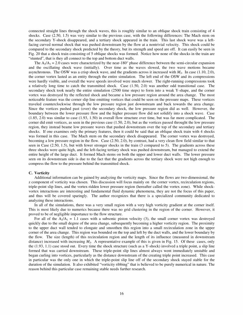
16

connected straight lines through the shock waves, this is roughly similar to an oblique shock train consisting of 4

shocks. Case (2.50, 1.5) was very similar to the previous case, with the following differences: The Mach stem on

the secondary Y-shock disappeared, and a tertiary shock appeared in the train. This last shock wave was a left-

facing curved normal shock that was pushed downstream by the flow at a nontrivial velocity. This shock could be

compared to the secondary shock predicted by the theory, but its strength and speed are off. It can easily be seen in

Fig. 20 that a shock train consisting of 5 oblique shocks was formed. Notice how none of the shocks in the train are

“stunted”, that is they all connect to the top and bottom duct walls.

The A2/A1 = 2.0 cases were characterized by the near-180° phase difference between the semi-circular expansion

and the oscillating shock wave (initially). Over time as the waves slowed, the two wave motions became

asynchronous. The OSW was a crisp shock wave, and the gradients across it increased with MS. In case (1.10, 2.0),

the corner vortex lasted as an entity through the entire simulation. The left end of the OSW and its compressions

were hardly visible, and overall the wave speeds involved were much slower. The right-running compressions took

a relatively long time to catch the transmitted shock. Case (1.50, 2.0) was another odd transitional case. The

secondary shock took nearly the entire simulation (2500 time steps) to form into a weak Y-shape, and the corner

vortex was destroyed by the reflected shock and became a low pressure region around the area change. The most

noticeable feature was the corner slip line emitting vortices that could be seen on the pressure maps. These vortices

traveled counterclockwise through the low pressure region just downstream and back towards the area change.

Since the vortices pushed past (over) the secondary shock, the low pressure region did as well. However, the

boundary between the lower pressure flow and the higher pressure flow did not solidify into a shock wave. Case

(1.85, 2.0) was similar to case (1.93, 1.50) in overall flow structure over time, but was far more complicated. The

corner did emit vortices, as seen in the previous case (1.50, 2.0), but as the vortices passed throught the low pressure

region, they instead beame low pressure waves that pushed downstream over the top of the secondary and tertiary

shocks. If one examines only the primary features, then it could be said that an oblique shock train with 4 shocks

was formed in this case. The Mach stem on the secondary shock disappeared. The corner vortex was destroyed,

becoming a low pressure region in the flow. Case (2.50, 2.0), by contrast, had a very clean flow field similar to that

seen in Case (2.50, 1.5), but with fewer stronger shocks in the train (3 compared to 5). The gradients across these

three shocks were quite high, and the left-facing tertiary shock was pushed downstream, but managed to extend the

entire height of the large duct. It formed Mach stems on both the upper and lower duct walls. The lower pressure

seen on its downstream side is due to the fact that the gradients across the tertiary shock were not high enough to

compress the flow to the pressure behind the transmitted shock.

C. Vorticity Additional information can be gained by analyzing the vorticity maps. Since the flows are two-dimensional, the

z component of vorticity was chosen. This discussion will focus mainly on the corner vortex, recirculation regions,

triple-point slip lines, and the vortex-ridden lower pressure region (hereafter called the vortex zone). While shock-

vortex interactions are interesting and fundamental fluid dynamic phenomena, they are not the focus of this paper,

and thus will be covered sparingly. The author recognizes that there is a specialized community dedicated to

analyzing these interactions.

In all of the simulations, there was a very small region with a very high vorticity gradient at the corner itself.

This is most likely due to numerics because there was no grid clustering in the region of the corner. However, it

proved to be of negligible importance to the flow structure.

For all of the A2/A1 = 1.1 cases with a subsonic piston velocity (3), the small corner vortex was destroyed

quickly due to the small degree of the area change, subsequently becoming a higher vorticity region. The proximity

to the upper duct wall tended to elongate and smoothen this region into a small recirculation zone in the upper

corner of the area change. This region was bounded on the top and left by the duct walls, and the lower boundary by

the flow. The size (length) of this recirculation region and the length of its influence (measured in downstream

distance) increased with increasing MS. A representative example of this is given in Fig. 15. Of these cases, only

the (1.93, 1.1) case stood out. Every time the shock structure (such as a Y-shock) involved a triple point, a slip line

formed that was carried downstream. These triple-point slip lines almost always went immediately unstable and

began curling into vortices, particularly as the distance downstream of the creating triple point increased. This case

in particular was the only one in which the triple-point slip line off of the secondary shock stayed stable for the

duration of the simulation. It also exhibited “vorticity ribbing” that is believed to be purely numerical in nature. The

reason behind this particular case remaining stable needs further research.

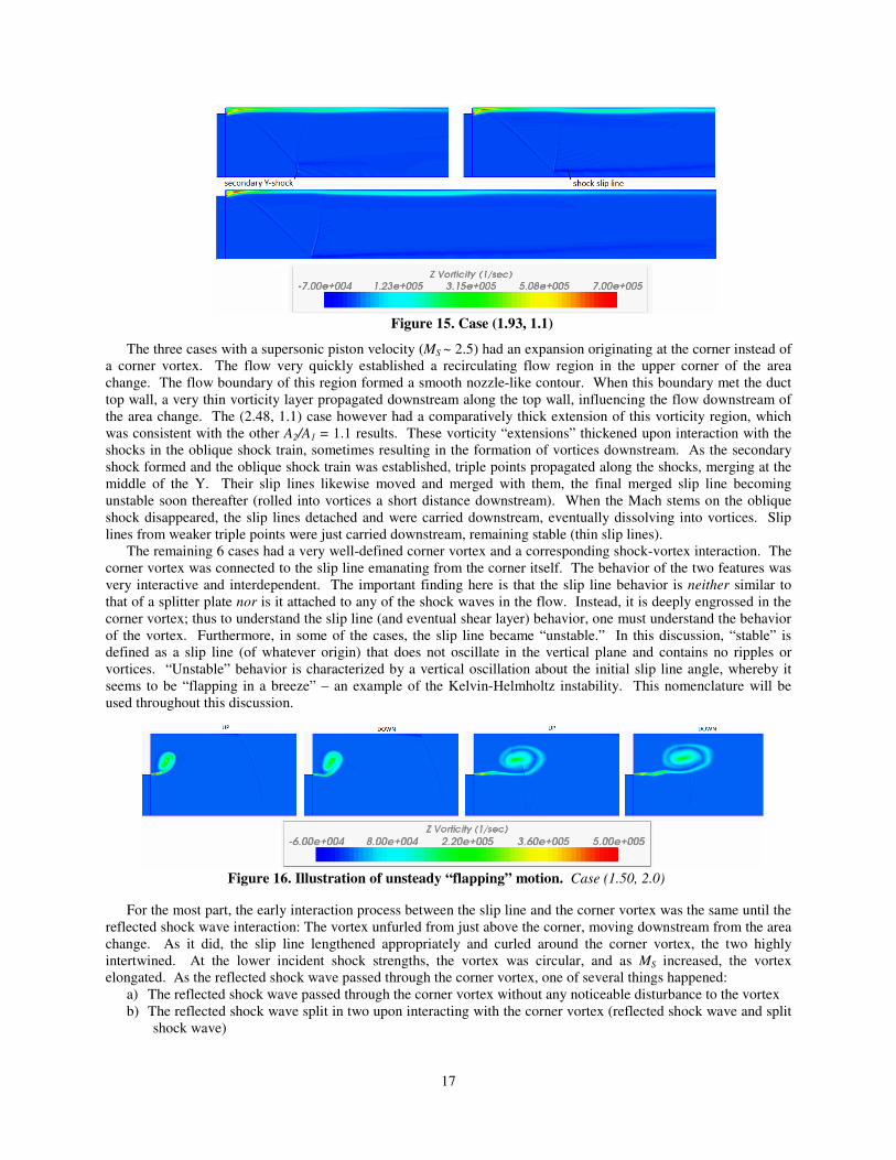
17

The three cases with a supersonic piston velocity (MS ~ 2.5) had an expansion originating at the corner instead of

a corner vortex. The flow very quickly established a recirculating flow region in the upper corner of the area

change. The flow boundary of this region formed a smooth nozzle-like contour. When this boundary met the duct

top wall, a very thin vorticity layer propagated downstream along the top wall, influencing the flow downstream of

the area change. The (2.48, 1.1) case however had a comparatively thick extension of this vorticity region, which

was consistent with the other A2/A1 = 1.1 results. These vorticity “extensions” thickened upon interaction with the

shocks in the oblique shock train, sometimes resulting in the formation of vortices downstream. As the secondary

shock formed and the oblique shock train was established, triple points propagated along the shocks, merging at the

middle of the Y. Their slip lines likewise moved and merged with them, the final merged slip line becoming

unstable soon thereafter (rolled into vortices a short distance downstream). When the Mach stems on the oblique

shock disappeared, the slip lines detached and were carried downstream, eventually dissolving into vortices. Slip

lines from weaker triple points were just carried downstream, remaining stable (thin slip lines).

The remaining 6 cases had a very well-defined corner vortex and a corresponding shock-vortex interaction. The

corner vortex was connected to the slip line emanating from the corner itself. The behavior of the two features was

very interactive and interdependent. The important finding here is that the slip line behavior is neither similar to

that of a splitter plate nor is it attached to any of the shock waves in the flow. Instead, it is deeply engrossed in the

corner vortex; thus to understand the slip line (and eventual shear layer) behavior, one must understand the behavior

of the vortex. Furthermore, in some of the cases, the slip line became “unstable.” In this discussion, “stable” is

defined as a slip line (of whatever origin) that does not oscillate in the vertical plane and contains no ripples or

vortices. “Unstable” behavior is characterized by a vertical oscillation about the initial slip line angle, whereby it

seems to be “flapping in a breeze” – an example of the Kelvin-Helmholtz instability. This nomenclature will be

used throughout this discussion.

For the most part, the early interaction process between the slip line and the corner vortex was the same until the

reflected shock wave interaction: The vortex unfurled from just above the corner, moving downstream from the area

change. As it did, the slip line lengthened appropriately and curled around the corner vortex, the two highly

intertwined. At the lower incident shock strengths, the vortex was circular, and as MS increased, the vortex

elongated. As the reflected shock wave passed through the corner vortex, one of several things happened:

a) The reflected shock wave passed through the corner vortex without any noticeable disturbance to the vortex

b) The reflected shock wave split in two upon interacting with the corner vortex (reflected shock wave and split

shock wave)

Figure 15. Case (1.93, 1.1)

Figure 16. Illustration of unsteady “flapping” motion. Case (1.50, 2.0)

18

c) The reflected shock wave split the corner vortex in half (itself splitting as well), causing its eventual

dissolution

With these general flow features in mind, the discussion will proceed with a case-by-case analysis of the

individual differences. Case (1.30, 1.5) exhibited a small amplitude oscillating behavior in the corner slip line,

indicating the potential to become unstable. These oscillations simply caused the subsequent portions of the slip line

to “pass the ripple” until the ripple arrived at the vortex. The vortex moved counterclockwise inside the

recirculation region bounded by the slip line in the upper corner of the area change. As the vortex moved

downwards, it “pushed” the slip line downwards, causing it to “bulge” into the flow path. The outer boundary of the

slip line did not form a smooth flow contour. In case (1.55, 1.5), the corner vortex unfurled from the wall slightly

elongated. The angle the slip line made with the horizontal was ~0°, and a small amplitude oscillation set in. The

oscillations caused the slip line to “bunch up” into small “packets of vorticity” that propagated along it, and they

interacted with the vorticity field created by the corner vortex. The small vortices, always moving

counterclockwise, continuously pushed downstream, thereby growing the recirculating region. The final vertical

thickness of the recirculation region was almost equal to the height difference between the two ducts. In case

(1.93, 1.5), the corner vortex again began oval-shaped, but the passage of the reflected shock wave seemed to initiate

the instability in the slip line. The slip line was angled upwards (~10°) and oscillated about this angle. The corner

vortex quickly dissipated into the recirculation region, whose flow boundary formed a shape similar to that of a

smoothly diverging nozzle. This region continuously pushed downstream, in contrast to the previous cases where it

always recirculated back towards the area change. To be more correct, the rate at which this vorticity zone pushed

downstream exceeded the rate at which it recirculated. In Fig. 26, notice how the oblique shocks in the shock train

do not meet the top wall, but are instead bounded by this vorticity zone. The author believes that is this the gas-

dynamic mechanism through which the lower pressure flow can invade the higher pressure region. This particular

finding (this “gas-dynamic pathway”) could be important for creating flow induction in the transient inlet concept.

Case (1.10, 2.0) began with a perfectly round corner vortex that was not affected by the passage of the reflected

shock wave. The slip line, however, exhibited a very slow (long period) oscillation. The oscillation did not cause

the slip line to “ripple”, but it did warp and curve. The flow did not create a recirculation region; instead, the slip

line simply curled around the corner vortex. Case (1.50, 2.0) is one of the most interesting cases because the full-

solution pressure fields reveal that the corner emitted vortices. The corner vortex was initially highly elongated,

curling upwards from the corner. It was obvious for this particular case that the reflected shock wave caused the

instability in the slip line because it caused the initial downward stroke in the slip line oscillation. Almost

immediately afterwards, the slip line rebounded and began emitting vorticity ripples that quickly evolved into

vortices that propagated along the slip line towards the corner vortex. These vortices moved counterclockwise

around the vortex and deformed it, as well as pushed further downstream, lengthening the recirculation region.

Furthermore, these vortices demonstrated a strong interaction with the secondary shock wave: each new vortex

caused a “crease” in the left branch of the secondary shock, which in turn created a triple point and attached slip

line. The triple point slip lines curled around the vortices moving downstream (dark blue in Fig. 28). This was the

second case in which these downstream-moving vortices restricted the secondary shock and allowed the lower

pressure flow to move over it. Case (1.85, 2.0) was very similar to that of (1.50, 2.0), having similar developments

over time. It was noticed that the interaction with the reflected shock wave is what caused the instability in the slip

line. The corner vortex elongated and deformed, forming the recirculation region. The slip line was sharply angled

upwards (~25-30°) and emitted vortices that behaved as described above. These vortices interacted with the

secondary and tertiary shocks in a similar manner. As these vortices moved downstream, they invaded the flow

beneath them, demonstrating the third and final occurrence of the gas-dynamic pathway.

A short summary of the pertinent observations from the discussion on vorticity follows:

a) Cases (1.30, 1.5) and (1.10, 2.0) were the only cases in which the corner vortex survived the entire

simulation.

b) Cases (1.93, 1.5), (1.50, 2.0), and (1.85, 2.0) were the only cases in which the vorticity region along the duct

upper wall seemed to provide a gas-dynamic pathway for the lower pressure flow surrounding the area

change region to overflow the oblique shock train and move downstream into the higher pressure flow

behind the transmitted shock wave.

c) In Cases (1.50, 2.0) and (1.85, 2.0), the corner emitted individual and distinct vortices that were visible in

both the pressure and vorticity maps.

d) The present simulations suggest that the passage of the reflected shock wave is the cause of the instability in

the corner slip line for all 6 cases, rather than being naturally unstable. [HYPOTHESIS NEEDS MORE

SUPPORT]

19

Figure 17. Full-Solution Pressure Map for Case (1.93, 1.1)

Figure 18. Full-Solution Pressure Map for Case (2.48, 1.1)

Figure 19. Full-Solution Pressure Map for Case (1.93, 1.5)

20

Figure 20. Full-Solution Pressure Map for Case (2.50, 1.5)

Figure 21. Full-Solution Pressure Map for Case (1.50, 2.0)

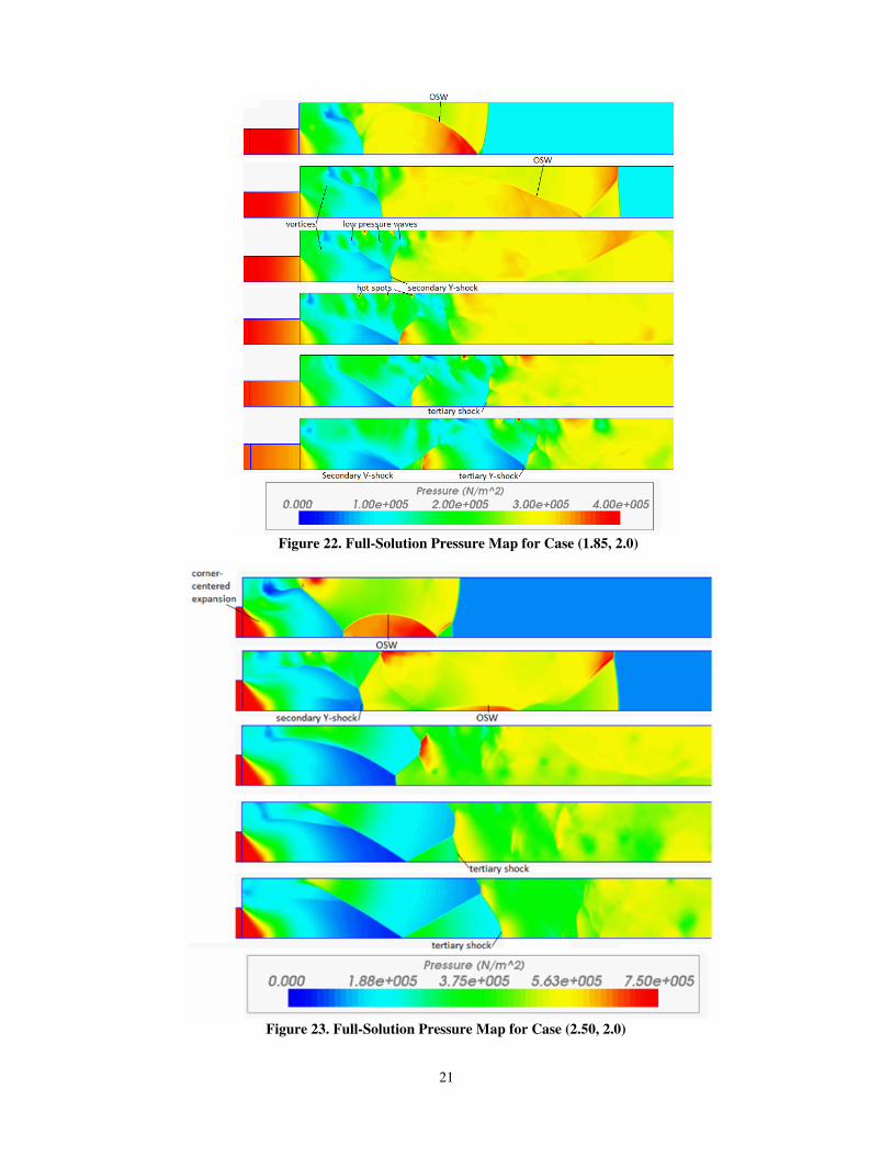
21

Figure 22. Full-Solution Pressure Map for Case (1.85, 2.0)

Figure 23. Full-Solution Pressure Map for Case (2.50, 2.0)

22

Figure 24. Case (1.30, 1.5)

Figure 25. Case (1.55, 1.5)

Figure 26. Case (1.93, 1.5)

23

V.

Figure 27. Case (2.50, 1.5)

Figure 28. Case (1.50, 2.0)

Figure 29. Case (1.85, 2.0)

24

V. Quantitative Results and Discussion

First the theoretical results will be discussed quantitatively in terms of the three primary wave strengths. Then,

these will be compared to the appropriate numerical results. Finally, some key paramters from the literature will be

computed and discussed, such as the critical shock location and the decay profile of the transmitted shock wave.

A. Theoretical

The main results from the theoretical analyses are the primary wave strengths: transmitted shock, reflected

expansion, and secondary shock. The transmitted shock is the shock that propagates from the injector duct into the

main engine duct, so predicting its strength is relevant to the application. The same holds true for the secondary

shock. Figs. 31-33 below show how these wave strengths are functions of incident shock strength and area ratio for

the given parameter space.

Figure 30. Case (2.50, 2.0)

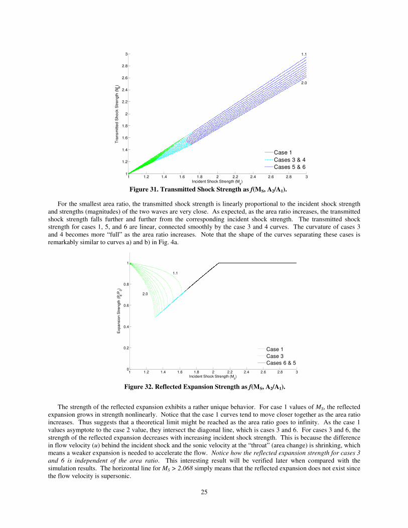
25

For the smallest area ratio, the transmitted shock strength is linearly proportional to the incident shock strength

and strengths (magnitudes) of the two waves are very close. As expected, as the area ratio increases, the transmitted

shock strength falls further and further from the corresponding incident shock strength. The transmitted shock

strength for cases 1, 5, and 6 are linear, connected smoothly by the case 3 and 4 curves. The curvature of cases 3

and 4 becomes more “full” as the area ratio increases. Note that the shape of the curves separating these cases is

remarkably similar to curves a) and b) in Fig. 4a.

The strength of the reflected expansion exhibits a rather unique behavior. For case 1 values of MS, the reflected

expansion grows in strength nonlinearly. Notice that the case 1 curves tend to move closer together as the area ratio

increases. Thus suggests that a theoretical limit might be reached as the area ratio goes to infinity. As the case 1

values asymptote to the case 2 value, they intersect the diagonal line, which is cases 3 and 6. For cases 3 and 6, the

strength of the reflected expansion decreases with increasing incident shock strength. This is because the difference

in flow velocity (u) behind the incident shock and the sonic velocity at the “throat” (area change) is shrinking, which

means a weaker expansion is needed to accelerate the flow. Notice how the reflected expansion strength for cases 3

and 6 is independent of the area ratio. This interesting result will be verified later when compared with the

simulation results. The horizontal line for MS > 2.068 simply means that the reflected expansion does not exist since

the flow velocity is supersonic.

1 1.2 1.4 1.6 1.8 2 2.2 2.4 2.6 2.8 31

1.2

1.4

1.6

1.8

2

2.2

2.4

2.6

2.8

3

Incident Shock Strength (Ms)

Tra

nsm

itte

d S

ho

ck S

tre

ng

th (

Mts

)

Case 1

Cases 3 & 4

Cases 5 & 6

2.0

1.1

Figure 31. Transmitted Shock Strength as f(MS, A2/A1).

1 1.2 1.4 1.6 1.8 2 2.2 2.4 2.6 2.8 30

0.2

0.4

0.6

0.8

1

Incident Shock Strength (Ms)

Exp

an

sio

n S

tre

ng

th (

P 8/P

3)

Case 1

Case 3

Cases 6 & 5

2.0

1.1

Figure 32. Reflected Expansion Strength as f(MS, A2/A1).

26

The left-facing secondary shock only exists for cases 3-6, where it is stationary for cases 3 and 4, and pushed

downstream for cases 5 and 6. Its purpose is to compress the expanded flow leaving the area change to the post-

transmitted-shock conditions. For cases 3 & 4, its strength increases with increasing MS due to the higher amount of

energy in the flow. Notice that is possible for the secondary shock to be stronger than the incident shock for the

larger area ratios. For cases 5 & 6, its strength decreases with increasing MS.

B. Comparison to Theory The primary wave strengths can be extracted from the simulations with some finesse, and they are compared to

the appropriate theoretical results. In general, the transmitted shock and the reflected expansion exhibit pretty good

agreement with the theory, but the results differ dramatically concerning the secondary shock wave. This, as will be

shown later, is due to the multidimensional nature of these flows.

First consider the strength of the transmitted shock. The computational results (12 total) for the transmitted

shock strength were obtained in the following manner: The data was sampled along the bottom wall at every 12th

time step. The bottom wall was chosen because this would be the “axis of symmetry” in a symmetric geometry (for

the purpose of comparison to the literature). At each time step for a given case, the location of the transmitted shock

1 1.2 1.4 1.6 1.8 2 2.2 2.4 2.6 2.8 31

1.2

1.4

1.6

1.8

2

2.2

2.4

2.6

2.8

3

Incident Shock Strength (Ms)

Se

co

nd

ary

Sh

ock S

tre

ng

th (

M ss)

Cases 3 & 4

Cases 5 & 6

1.1

2.0

Figure 33. Secondary Shock Strength as f(MS, A2/A1).

1 1.2 1.4 1.6 1.8 2 2.2 2.4 2.6 2.8 31

1.2

1.4

1.6

1.8

2

2.2

2.4

2.6

2.8

3s 2 1

Incident Shock Strength (Ms)

Tra

nsm

itte

d S

ho

ck S

tre

ng

th (

M ts)

A2/A

1 = 1.1, theor.

A2/A

1 = 1.1, comp.

A2/A

1 = 1.5, theor.

A2/A

1 = 1.5, comp.

A2/A

1 = 2.0, theor.

A2/A

1 = 2.0, comp.

1.1

2.0

1.5

Figure 34. Transmitted Shock Strength – Comparison of Numerical and Theoretical Results

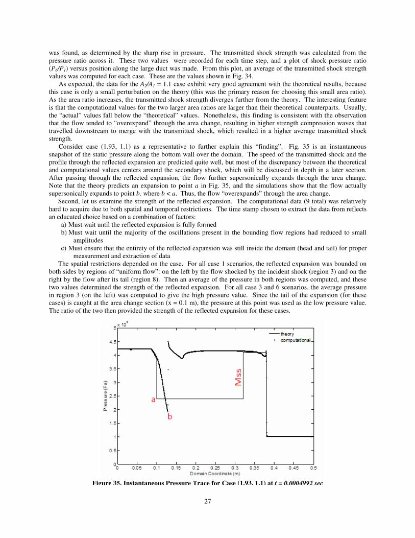
27

was found, as determined by the sharp rise in pressure. The transmitted shock strength was calculated from the

pressure ratio across it. These two values were recorded for each time step, and a plot of shock pressure ratio

(P6/P1) versus position along the large duct was made. From this plot, an average of the transmitted shock strength

values was computed for each case. These are the values shown in Fig. 34.

As expected, the data for the A2/A1 = 1.1 case exhibit very good agreement with the theoretical results, because

this case is only a small perturbation on the theory (this was the primary reason for choosing this small area ratio).

As the area ratio increases, the transmitted shock strength diverges further from the theory. The interesting feature

is that the computational values for the two larger area ratios are larger than their theoretical counterparts. Usually,

the “actual” values fall below the “theoretical” values. Nonetheless, this finding is consistent with the observation

that the flow tended to “overexpand” through the area change, resulting in higher strength compression waves that

travelled downstream to merge with the transmitted shock, which resulted in a higher average transmitted shock

strength.

Consider case (1.93, 1.1) as a representative to further explain this “finding”. Fig. 35 is an instantaneous

snapshot of the static pressure along the bottom wall over the domain. The speed of the transmitted shock and the

profile through the reflected expansion are predicted quite well, but most of the discrepancy between the theoretical

and computational values centers around the secondary shock, which will be discussed in depth in a later section.

After passing through the reflected expansion, the flow further supersonically expands through the area change.

Note that the theory predicts an expansion to point a in Fig. 35, and the simulations show that the flow actually

supersonically expands to point b, where b < a. Thus, the flow “overexpands” through the area change.

Second, let us examine the strength of the reflected expansion. The computational data (9 total) was relatively

hard to acquire due to both spatial and temporal restrictions. The time stamp chosen to extract the data from reflects

an educated choice based on a combination of factors:

a) Must wait until the reflected expansion is fully formed

b) Must wait until the majority of the oscillations present in the bounding flow regions had reduced to small

amplitudes

c) Must ensure that the entirety of the reflected expansion was still inside the domain (head and tail) for proper

measurement and extraction of data

The spatial restrictions depended on the case. For all case 1 scenarios, the reflected expansion was bounded on

both sides by regions of “uniform flow”: on the left by the flow shocked by the incident shock (region 3) and on the

right by the flow after its tail (region 8). Then an average of the pressure in both regions was computed, and these

two values determined the strength of the reflected expansion. For all case 3 and 6 scenarios, the average pressure

in region 3 (on the left) was computed to give the high pressure value. Since the tail of the expansion (for these

cases) is caught at the area change section (x = 0.1 m), the pressure at this point was used as the low pressure value.

The ratio of the two then provided the strength of the reflected expansion for these cases.

Figure 35. Instantaneous Pressure Trace for Case (1.93, 1.1) at t = 0.0004992 sec

28

The computational results show rather good agreement with the theoretical results, as shown in Fig. 36. The

strength of the reflected expansion first increases then decreases in strength as the incident shock strength increases.

They validate the conclusion that for cases 3 and 6, the strength of the reflected expansion is independent of the area

ratio.

Third, the secondary shock strength is the largest difference between the theoretical predictions and the

computational results. Recall that the secondary shock only exists for cases 3-6 (case 4 does not exist for the area

ratios under consideration here), where case 3 has a standing shock and cases 5 and 6 have moving secondary

shocks. The data (9 total) was taken along the bottom wall at the end of each simulation. This was done to allow

oscillations to dampen out and all primary flow features to establish their “constant” speeds and strengths.

Theoretically, the case 3 algorithm assumes a “continuous” area change accomplished via a short nozzle and that

the secondary shock stands somewhere in the area change section. Furthermore, the flow partially expands before

and after the secondary shock. Realistically, in a discontinuous area change, this means that the secondary shock

will stand somewhere just downstream of the area change. But the flow still partially expands before and partially

expands after the secondary shock. This makes extracting its strength quite diffucult without a large degree of error.

The computational data was taken across the shock only, meaning that the pressures at points on either side of the

numerical shock were used in the calculation of its strength.

For cases 5 and 6, the measurement is made difficult by the fact that the flow usually involves more than one

shock to accomplish the compression process, the oblique nature of the shocks, the presence of Mach stems and

shock trains, and other 2D phenomena (discussed above). Thus, the only way to extract a measurement is to return

to the purpose of the secondary shock: to shock the supersonically expanded flow from the area change to the

pressure behind the transmitted shock. The low pressure value was taken from the supersonically expanding flow

just to the left of the secondary shock. This point is the “left boundary” of the flow entering the “secondary shock”.

The high pressure value was computed as an average of the flow pressure between the transmitted shock (having

already left the domain) and the last shock in the train (regions 6 and 7 from theory). This flow region is the “right

boundary” of the flow leaving the “secondary shock”. From the ratio of these two values, the Mach Number of the

secondary shock is computed. The results are summarized in Fig. 37.

Due to the methods used to calculate MSS, the results are not unexpected. The results for case 3 are lower than

their theoretical values because only the numerical shock was measured. The results for cases 5 and 6 are far larger

than their theoretical values due to a combination of factors: First, because the flow overexpanded through the area

change, the first oblique shock in the train was of much higher strength than predicted. Hence the “low pressure”

boundary was lower than expected. Second, the pressure behind the transmitted shock was higher than predicted,

which means that the “high pressure” boundary was higher than expected.

1 1.2 1.4 1.6 1.8 2 2.2 2.4 2.6 2.8 30

0.2

0.4

0.6

0.8

1

Incident Shock Strength (Ms)

Exp

an

sio

n S

tre

ng

th (

P 8/P

3)

A2/A

1 = 1.1, theor.

A2/A

1 = 1.1, comp.

A2/A

1 = 1.5, theor.

A2/A

1 = 1.5, comp.

A2/A

1 = 2.0, theor.

A2/A

1 = 2.0, comp.

Figure 36. Reflected Expansion Strength: Comparison of Numerical and Theoretical Results

29

Looking at Fig. 37, even though the magnitudes of the results differ greatly, the trends are mostly present. That

is, the computational data first increase then decrease with increasing MS. This holds except for the (2.50, 2.0) case,

which does not decrease. This is due to the fact that the flow expanded too low before the first oblique shock in the

train.

Generally speaking, the secondary shock tended to be of much higher strength and yet of much slower speed

than the theory predicted. This is counterintuitive but can be explained via the multidimensionality. The flow

essentially traded a single, fast-moving normal shock for a (more-or-less) stationary oblique shock train. [NEED

TO FINISH THIS DISCUSSION OF RESULTS]

C. Identified Key Parameters This section considers parameters that have been identified by previous work to be important measures of these

flows. Data on these parameters is extracted from the current simulations to increase the body of work on these

topics. The two parameters analyzed here are the location of the critical shock and the decay of the transmitted

(axial) shock wave.

Critical Shock Location: Sloan and Nettleton 1975 did a theoretical and experimental study on 2 DOF (planar) and 3 DOF (cylindrical)

shocks entering a sudden area change. Most importantly, their results are for symmetrically expanding shock waves.

They establish the definition of the critical shock: “the critical shock is defined as the configuration when the

decaying shock wave at the axis [of symmetry] first becomes curved.” This is equivalent to the point at which an

originally planar shock becomes a spherically expanding shock. If the current geometry is mirrored about the

bottom wall, one finds that the two studies have comparable geometries. Hence, the “axis of symmetry” is the

bottom wall in these studies, and thus the data was taken along it (from the short simulations) only at every 12th

time

step. An important note for the data in this section and the next is that taking the data along the bottom wall only

records every other oscillation of the OSW.

The location of the critical shock is defined as the distance (in meters) downstream of the area change (here,

located at 0.1m from the left end of the domain) at which the decaying shock wave (the transmitted shock wave)

first becomes curved. The curvature will be noted by a decrease in the strength of the shock wave as indicated by

the ratio between the post-shock pressure and the initial pressure. These two definitions allowed for the location of

the critical shock to be determined.

1 1.2 1.4 1.6 1.8 2 2.2 2.4 2.6 2.8 31

1.5

2

2.5

3

Incident Shock Strength (Ms)

Se

co

nd

ary

Sh

ock S

tre

ng

th (

M ss)

A2/A

1 = 1.1, theor.

A2/A

1 = 1.1, comp.

A2/A

1 = 1.5, theor.

A2/A

1 = 1.5, comp.

A2/A

1 = 2.0, theor.

A2/A

1 = 2.0, comp.

Figure 37. Secondary Shock Strength: Comparison of Numerical and Theoretical Results

30

At every 12th

time step, the location of the transmitted shock was found via the peak pressure behind the

transmitted shock. The location and magnitude (strength) of this peak were recorded for each time step, and these

values were plotted over the domain. The first portion of this plot (plateau and decay) was used for these

calculations. An average value for the post-shock pressure (the “plateau”) was computed, and a 5th

order polynomial

was curve-fit to the “decay” portion. The x-coordinate of the intersection of these two lines is the critical shock

location. This method is similar to the method used in Sloan and Nettles 1975: they used the intersection between

the two linear curve fits to determine the critical shock location. An example of the current methodology is

presented in Fig. 38. Using the stated methods, the data from the original set of 12 simulations (taken along the

bottom wall) produced the results in Fig 39.

There are a few noticeable trends: the critical shock location moves further downstream as the area ratio

increases, and that it seems to first decrease then increase with MS. The current understanding of the transmitted

shock decay is that rays (single rarefaction waves) originate at a point and propagate towards the moving shock, and

upon contact, curve it. Using the hypothesis that the decay is due to interactions with an expansion, one can provide

justification to these trends.

Decay Profile of the Transmitted Shock:

The second key parameter is the decay profile of the transmitted shock. This parameter describes how the

transmitted shock decays as it passes through the area change. Recall that this is the shock wave that will enter the

main engine duct and propagate downstream, so understanding its behavior is of practical importance. These results

will be presented in two parts: First, the initial decay of the transmitted shock will be compared to the literature.

Then it will be shown that the transmitted shock undergoes a series of boosts to its strength until its final strength is

reached. This final strength is higher than that seen when only considering the shock decay. The authors have not

observed this phenomenon documented in the literature.

First consider the initial decay profile of the transmitted shock as it moves downstream. As seen before in the

critical shock location results, there are two parts to this curve: the initial plateau as the shock propagates through

the area change (without diffracting at the axis), and the subsequent decay as the shock curves and the flow behind it

expands. Nettleton 1973 and Sloan and Nettleton 1975 discuss the decay of the “axial shock”. Nettleton 1973

examined a “gradual” (continuous) area change over a range of divergent angles of 5° to 90°, and found that the

results for the 90° angle diverged significantly from the theoretical results, as well as that a curved corner did not

significantly affect the strength of the transmitted shock. Sloan and Nettleton 1975 examined a discontinuous

symmetric 90° area change for both planar (2 DOF) and cylindrical (3 DOF) incident shocks. Their results are

presented below for comparison.

In order to examine the initial decay profile, the data was taken along the bottom wall for each case at every 12th

time step (recall, this records every other oscillation of the OSW). All four long cases (5000 time steps) were used

in place of their short counterparts (2500 time steps) to enhance the quality of the data. The data was taken from the

area change (at x = 0.1m) to the first compression wave that interacted with the transmitted shock.

Now consider the results over the entire simulation time, instead of just the first portions. After the transmitted

shock undergoes the initial decay due to the area change, it experiences a series of subsequent boosts to its strength.

This process takes place as a series of initial compression waves followed by expansions. This lends further

credence to the hypothesis that the semi-circular expansion and OSW bounce between the upper and lower duct

walls, interacting with each other to create alternating regions of lower and higher pressure flow. To visualize this,

see Fig. 44. Each jump is due to a right-running oblique compression wave or oblique shock merging with the

transmitted shock. Each decay is due to the two-dimensional pieces of the semi-circular expansion. As the

gradients across the OSW grow, the compression waves steepen into shock waves. Over time, as the OSW and SCE

lose strength, so do the compressions and expansions sent upstream and downstream. Thus, each subsequent jump

and decay have smaller amplitudes than the previous set, until eventually the pressure magnitude settles out to a

roughly constant value. This behavior is very similar to an overdamped system. This is the value used to calculate

the transmitted shock strength to compare to the theoretical results. It be noted, however, that in most cases, a

sufficiently long enough time was not reached to obtain this constant value.

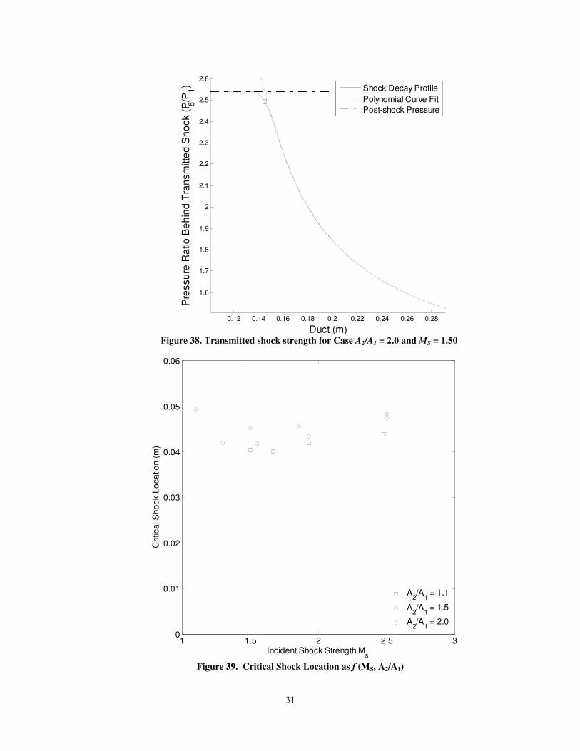
31

0.12 0.14 0.16 0.18 0.2 0.22 0.24 0.26 0.28

1.6

1.7

1.8

1.9

2

2.1

2.2

2.3

2.4

2.5

2.6

2 1 s

Duct (m)

Pre

ssu

re R

atio

Be

hin

d T

ran

sm

itte

d S

ho

ck (

P 6/P

1)

Shock Decay Profile

Polynomial Curve Fit

Post-shock Pressure

Figure 38. Transmitted shock strength for Case A2/A1 = 2.0 and MS = 1.50

1 1.5 2 2.5 30

0.01

0.02

0.03

0.04

0.05

0.06

Incident Shock Strength Ms

Critic

al S

ho

ck L

oca

tion

(m

)

A2/A

1 = 1.1

A2/A

1 = 1.5

A2/A

1 = 2.0

Figure 39. Critical Shock Location as f (MS, A2/A1)

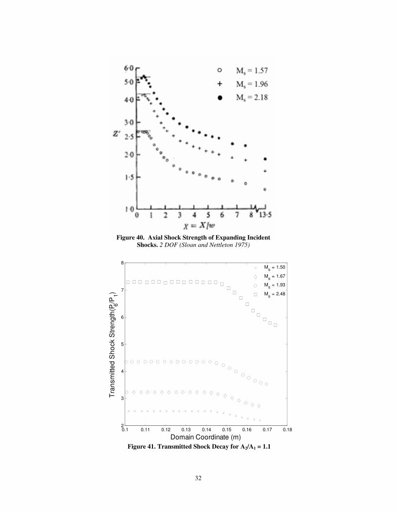
32

Figure 40. Axial Shock Strength of Expanding Incident

Shocks. 2 DOF (Sloan and Nettleton 1975)

0.1 0.11 0.12 0.13 0.14 0.15 0.16 0.17 0.182

3

4

5

6

7

82 1

Domain Coordinate (m)

Tra

nsm

itte

d S

ho

ck S

tre

ng

th(P

6/P

1)

M

s = 1.50

Ms = 1.67

Ms = 1.93

Ms = 2.48

Figure 41. Transmitted Shock Decay for A2/A1 = 1.1

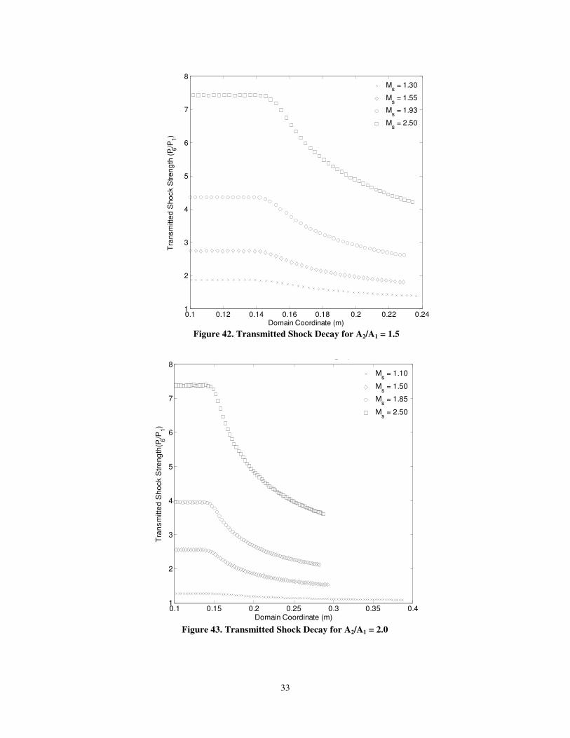
33

0.1 0.12 0.14 0.16 0.18 0.2 0.22 0.241

2

3

4

5

6

7

82 1

Domain Coordinate (m)

Tra

nsm

itte

d S

ho

ck S

tre

ng

th (

P 6/P

1)

Ms = 1.30

Ms = 1.55

Ms = 1.93

Ms = 2.50

Figure 42. Transmitted Shock Decay for A2/A1 = 1.5

0.1 0.15 0.2 0.25 0.3 0.35 0.41

2

3

4

5

6

7

82 1

Domain Coordinate (m)

Tra

nsm

itte

d S

ho

ck S

tre

ng

th(P

6/P

1)

Ms = 1.10

Ms = 1.50

Ms = 1.85

Ms = 2.50

Figure 43. Transmitted Shock Decay for A2/A1 = 2.0

34

VI. Conclusion

In summary, this study analyzed the interaction between a shock wave and a discontinuous area enlargement

using theoretical and numerical techniques. For the given parameter space (MS, A2/A1), there are 6 possible wave

patterns primarily involving a transmitted shock wave, an expansion reflected from the interaction, and a secondary

shock wave. The 1-D theory provided a framework to analyze the numerical simulations. The primary wave

strengths are computed both theoretically and numerically, and these results are compared. In addition, the

simulations provided insight into the two-dimensional nature of these flows via pressure and vorticity scalar maps

that revealed interesting features such as shock structure, shock-vortex interactions, vorticies, and expansions.

Some conclusions that can be drawn from this study are: First, the theory predicts the transmitted shock and

reflected expansion strengths rather well, but fails to predict the secondary shock strength. Second, the transmitted

shock wave does not just decay as the literature suggests, but also experiences modifications that serve to increase

its strength until a final (higher) strength is reached. This final strength is comparable to the theoretical values.

Third, that geometries with discontinuous area changes cannot be accurately modeled by quasi-1D methods due to

the highly two-dimensional nature of these flows.

This parametric study contributed the following findings to the scientific knowledgebase: First, the presence of

the oscillating shock wave (OSW), its behavior, and how it affects the shock structure. Second, the prescence of the

semi-circular expansion and its role as the origin of the reflected expansion. Third, how the multidimensional

interaction between these two features creates the prominent flow features present in these flows. Fourth, a new

definition of the time to reach quasi-1D flow is offered, based on the behavior of the oscillating shock wave.

Finally, a vorticity layer containing vortices that pushed downstream was discovered. This vorticity layer can

provide a fluid-dynamic pathway for lower pressure flow to encroach into higher pressure flow, which could be

important to the application by providing a means for flow induction into the engine.

Further research is needed to determine under what conditions the following occur: when the reflected shock will

not destroy the corner vortex, when the slip lines generated by the triple points in the shock structures are inviscidly

stable, and when the corner will begin emitting vortices. The results could lead to some interesting applications of

active flow control.

Appendix

As mentioned above, a summary of the numerical settings used for the 16 simulations is presented here:

Table 2. Reference Conditions

Quantity Value

TREF 300 K

PREF 101325 Pa

VREF 347.128 m/s

LREF 0.5 m / *0.7 m

a) b) c)

Figure 44. Transmitted Shock Decay Profile over Domain. a) (2.48, 1.1) b) (2.50, 1.5) c) (2.50, 2.0)

35

Table 3. Numerical Settings (* denotes a long case)

A2/A1 MS Case Run time Time step Total # grid pts

1.1 1.50 1 06 hr 15 min 5e-07 sec 152,274

1.1 1.67 3 06 hr 21 min 5e-07 sec 152,274

1.1 1.93 6 06 hr 36 min 4e-07 sec 152,274

1.1 2.48 5 06 hr 19 min 3e-07 sec 152,274

1.5 1.30 1 08 hr 41 min 6e-07 sec 197,596

1.5 1.55 3 09 hr 02 min 5e-07 sec 197,596

1.5 1.93 6 09 hr 25 min 4e-07 sec 197,596

*1.5 1.93 6 16 hr 34 min 4e-07 sec 282,178

1.5 2.50 5 09 hr 04 min 3e-07 sec 197,596

*1.5 2.50 5 16 hr 49 min 3e-07 sec 282,178

2.0 1.10 1 09 hr 42 min 7e-07 sec 253,582

2.0 1.50 3 10 hr 30 min 5e-07 sec 253,582

2.0 1.85 6 10 hr 47 min 4e-07 sec 253,582

*2.0 1.85 6 21 hr 29 min 4e-07 sec 366,136

2.0 2.50 5 10 hr 24 min 3e-07 sec 253,582

*2.0 2.50 5 21 hr 57 min 3e-07 sec 366,136

References

CURVING/TURNING DUCTS: 1Igra, O., Falcovitz, J., Meguro, T., Takayama, K., and Heilig, W. (1999) Shock Wave Propagation through a double bend

duct. Proc. Of the 22nd Int. Symposium of Shock Waves, Imperial College, London. 2Liang, S. M., Weng, K. C., and Takayama, K. Numerical Study of Blast-wave propagation in a double-bent duct. AIAA vol

40 no 9 2002. 3Edwards, D. H., Fearnley, P., and Nettleton, M. A. Shock Diffraction in channels with 90° bends. J. Fluid Mech. (1983) vol

132, pg. 257-270. 4Takayama, K., Honda, M., Onodera, O. Shock Propagation along 90 degree bends. Instn. High Speed Mech. Report 1976

vol 35 pg. 83-111 5Sommerfeld, M., Nishida, M., and Takayama, K. (1985) Shock propagation in a curved duct. Instn. High Speed Mech.

Report, Tohoku University, Sendai, Japan. 6Kage, K., Shiroyama, M., and Ishimatsu, K. Numerical study of shock waves propagating through right angled multiple

elbows. J. Thermal Science, vol 14 no 3

LARGE ANGLES/CORNERS: 7Skews, B. W. The Perturbed Region behind a diffracting shock wave. J. Fluid Mech (1967), vol. 29 part 4, pgs. 705-719. 8Skews, B. W. The Shape of a Diffracting Shock Wave. J. Fluid Mech. (1967) vol. 29 part 2, pgs. 297-304. 9Sun, M. and Takayama, K. Vorticity Production in Shock Diffraction. J. Fluid Mech. (2003) vol 478, pgs. 237-256. 10Bazhenova, T. V., Gvozdeva, L. G., and Zhilin, Yu. V. Change in the Shape of the Diffracting Shock Wave at a Convex

Corner. Acta Astronautica, Vol. 6, pgs. 401-412 11Dumitrescu, L. Z. and Preda, S. Some New Results Concerning the Diffraction of a Shock Wave Around a Convex Corner.

Modern Developments in Shock Tube Research: Proceedings of the 10th International Shock Tube Symposium 1975, pgs. 369-

377. Editor: G. Kamimoto

BRANCHED DUCTS: 12Heilig, W. (1975) Propagation of shock waves in various branched ducts. Proc. of the 10th Int. Shock Tube Symposium,

Kyoto Japan. 13Hammitt, A. G., and Carpenter, H. J. (1964) Unsteady flow past junctures in ducts. AIAA 2, 2224 14Igra, O., Wang, L., Falcovitz, J., and Heilig, W. (1998c) Shock Wave propagation in a branched duct. Shock Waves, 8, 375-

381. 15Deckker, B. E. L., and Male, D. H. Unsteady Flow in a Branched Duct. Proc. Instn Mech. Engrs. 1968 Vol 182 Paper 10

36

16Deckker, B. E. L., and Male, D. H. Fluid Dynamic Aspects of Unsteady Flow in Branched Ducts. Proc. Instn Mech. Engrs.

1968 Vol 182 Paper 18 17Zimmerman, A. W., Peterson, J. B., and Carpenter, H. J. Nonsteady flow past duct junctures. AIAA vol 7 no 3

BAFFLES/OBSTACLES: 18Reichenbach, H., and Kuhl, A. L. (1993) Shock-induced turbulent flow in baffle systems. Proc. Of 16th Int. Symposium on

Shock Tubes and Waves, Aachen, 847-853. 19Kuhl, A. L. and Reichenbach, H. Flow visualization of shock propagation in baffle systems. Ernst-Mach-Institute. 20Berger, S., Sadot, O., and Ben-Dor, G. Experimental investigation on the shock-wave load attenuation by geometrical

means. Shock Waves (2010) 20: 29-40. 21Graham, J. M. R. and Hillier, R. Shock wave diffraction at a sharp edge and the effect of baffles in a shock tube. proc. of

the 13th Int. Symp. on Shock Tubes and Waves, pg. 402-410 22Ohtomo, F., Ohtani, K., and Takayama, K. Attentuation of shock waves propagating over arrayed baffle plates. Shock

Waves (2005) Vol 14 no 5-6, pg. 379-390. 23Klapovskii, V. E., Mineev, V. N., Grigor’ev, G. S., Vershinin, V. Yu., Logvenov, A. Yu. Attenuation of an air shock wave

by perforated baffles. Combustion, Explosion, and Shock Waves, 1983, Volume 19, Number 5, Pages 638-639 24Gel’fand, B. E., Medvedev, S. P., Polenov, A. N., Tsyganov, S. A. Interaction of Unsteady pressure waves and perforated

baffles. Fluid Dynamics, 1987, Volume 22, Number 6, Pages 969-972 25Grin, V. T., Kraiko, A. N., and Miller, L. G. Decay of a shock wave at a perforated baffle. Journal of Applied Mechanics

and Technical Physics, 1981, Volume 22, Number 3, Pages 372-378 26Schultz-Grunow, F. Production and Inhibition of Mach Stems. Modern Developments in Shock Tube Research:

Proceedings of the 10th international Shock Tube Symposium, Kyoto, Japan, 1975. Kamimoto, G. pgs. 356-362

SHOCK WAVE FOCUSING: 27Inoue, O., Takahashi, N., and Takayama, K. Shock Wave focusing in a log-spiral duct. AIAA vol 31, no 6 1993 28Bond, C., Hill, D. J., Meiron, D. I., and Dimotakis, P. E. Shock focusing in a planar convergent geometry: experiment and

simulation. J. Fluid Mech. (2009) vol 641, pg. 297-333 29Setchell, R. E., Storm, E., and Sturtevant, B. An investigation of shock strengthening in a conical convergent channel. J.

Fluid Mech (1972) vol 56 part 3, pg. 505-522. 30Taieb, D., Ribert, G., Hadjadj, A. Numerical Simulations of shock focusing over concave surfaces. AIAA 2010 vol 48 no 8. 31Takayama, K. and Jiang, Z. Reflection and focusing of toroidal shock waves from co-axial annular shock tubes. AIAA-

1997-523 32Cramer, M. S. Focusing of a weak three-dimensional shock wave. AIAA 1981 vol 19 no 10 33Milton, B. E. and Archer, R. D. Generation of implosions by area change in a shock tube. AIAA 1969 vol 7 no 4. 34Hosseini, S. H. R. and Takayama, K. Experimental study of toroidal shock wave focusing in a compact vertical annular

diaphragmless shock tube. Shock Waves (2010) 20:1-7

MISCELLANEOUS: 35Ben-Dor, G., Igra, O., and Elperin, T. Handbook of Shock Waves. Academic Press: 2001 Vol 1-3 36Chester, W. The propagation of shock waves in a channel of non-uniform width. Quart. J. Mech. Appl. Math., 1953, 6, 440-

452 37Chester, W. The propagation of shock waves along ducts of varying cross-section. Adv. Appl. Mech. 1960, 6, 119-152 38Chisnell, R. F. The motion of a shock wave in a channel, with applications to cylindrical and spherical shock waves. J.

Fluid Mech. 1957, 2, 286-298. 39Whitham, G. B. A new approach to problems of shock dynamics: Part I Two-dimensional problems. J. Fluid Mech. 1957, 2,

146-171. 40Whitham, G. B. On the propagation of shock waves through regions of non-uniform area or flow. J. Fluid Mech. 1958, 4,

337-360. 41Whitham, G. B. A new approach to problems of shock dynamics: Part II three-dimensional problems. J. Fluid Mech. 1959,

5, 369-386.

SHOCK WAVES IN ALL OF THE BELOW: 42Schardin, H. and Reichenbach, H. The behavior of shock waves in ducts and when entering entrance structures. Proc.

Symposium on Protective Structures for Civilian Populations pg. 193-206 43Kahane, A., Warren, W. R., Griffith, W. C., and Marino, A. A. A Theoretical and Experimental Study of Finite Amplitude

Wave Interactions with Channels of Varying Area. J. Aeron. Sci. 1954 vol 21, no 8. 44Andrianov, N. and Warnecke, G. On the Solution to the Riemann Problem for the Compressible Duct Flow. SIAM J. Appl.

Mathem, vol 64, no 3, pg. 878-901. 45Yu, F. M. and Wang, C. Z. Study on the shock interference in a wedged convergent-divergent channel. Proc. of the 24th Int.

Symposium on Shock Waves, Beijing, China. Springer 2004. 46Hawken, D. F. and Gottlieb, J. J., Prediction of Two-Dimensional Time-Dependent Gasdynamic Flows for Hypersonic

Studies. UTIAS Report No. 335, March 1990 47Bazhenova, T. V., Gvozdeva, L. G., and Nettleton, M. A. Unsteady Interactions of Shock Waves. Prog. Aerospace Sci.

1984 Vol. 21 pgs. 249-331.

37

48Oshima, K. Some Flow Patterns Observed in Shock Tubes and the Comparison with Results by Numerical Simulation.

Modern Developments in Shock Tube Research: Proceedings of the 10th International Shock Tube Symposium 1975, pgs. 480-

487. Editor: G. Kamimoto

BOTH AREA ENLARGEMENTS AND REDUCTIONS (NOZZLE FLOWS): 49Amann, H. O., and Reichenbach, H. (1973) Unsteady flow phenomena in shock-tube nozzles. Proc. Of the 9th Int. Shock

Tube Symposium, Stanford, CA. 50Igra, O., Wang, L., Falcovitz, J., and Amann, H. O. (1998b) Simulation of the starting flow in a wedge-like nozzle. Shock

waves, 8, 235-242.

51Han, Z. and Yin, X. Shock Dynamics. Beijing Science Press 1993 52Rudinger, George. Wave Diagrams for Nonsteady Flow in Ducts. D. Van Nostrand Company: 1955 53Needham, C. E. and Crepeau, J. E. SHAMRC, Second-order Hydrodynamic Automatic Mesh Refinement Code. Rep.

Applied Research Associates (ARA) Inc., Albuquerque, NM, 1998 Vol. 2, User’s Manual. 54Falcovitz, J. and Ben-Artzi, M. Recent Developments of the GRP Method. Japan Soc. Mech. Engrs. Internat. J., Series B,

Vol. 38, No. 4, 1995, pgs. 497-517.

BOTH CONTINUOUS AREA ENLARGEMENTS AND REDUCTIONS: 55Igra, O., Elperin, T., Falcovitz, J., Zmiri, B. Shock Wave Interaction with Area Changes in Ducts. Shock Waves (1994)

3:233-238. (RCM) 56Greatrix, D. R. and Gottlieb, J. J., An Analytical and Numerical Study of a Shock Wave Interaction with an Area Change.

UTIAS Report No. 268, Nov. 1982

CONTINUOUS AREA ENLARGEMENT: 57Igra, O. and Falcovitz, J. Numerical solution to rarefaction or shock wave/duct area-change interaction. AIAA vol 24, no 8 58Nettleton, M. A. Shock Attenuation in a ‘Gradual’ Area Expansion. J. Fluid Mech. (1973), vol 60 part 2, pgs. 209-223.

CONTINUOUS AREA REDUCTIONS: 59Igra, O., Wang, L., and Falcovitz, J. (1998a) Nonstationary compressible flow in ducts with varying cross-section. Proc.

Instn. Mech. Engrs., 212, 225-243. 60Asano, N. Shock waves and non-stationary flow in a duct of varying cross-section. J. Fluid Mech. (1971) vol 46 part 1, pg.

111-128. 61Bird, G. A. The effect of wall shape on the degree of reinforcement of a shock wave moving into a converging channel. J.

Fluid Mech. Vol 5 part 1 pg. 60-66 62Russell, D. A. Shock-wave strengthening by area convergence. J. Fluid Mech. (1967), vol 27 part 2, pgs. 305-314. 63Ben-Dor,Gabi. Shock Wave Reflection Phenomena – 2nd Ed. Springer-Verlag 2010.

BOTH DISCONTINUOUS AREA ENLARGEMENTS AND REDUCTIONS: 64Menina, R., Saurel, R., Zereg, M., Houas, L. Modelling Gas Dynamics in 1D Ducts with Abrupt Area Change. Shock

Waves (2011), Volume 21, Number 5, Pages 451-466. 65Salas, Manuel. Shock Wave Interaction with an Abrupt Area Change. NASA Technical Report 3113. 1991

DISCONTINUOUS AREA REDUCTIONS: 66Falcovitz, J. and Igra, O. Model for shock interaction with sharp area reduction. Proc. of the 26th Int. Symposium on Shock

Waves, Vol. 1. Springer. Pg. 647-652. 67Rudinger, G. Passage of Shock Waves Through Ducts of Variable Cross Section. Physics of Fluids 1960, Vol 3 no 3. Pg.

449-455. 68Itoh, S., Kitamura, A., and Itaya, M. On the Profile of Reflected Shock and its Attenuation Process. Modern Developments

in Shock Tube Research: Proceedings of the 10th International Shock Tube Symposium 1975, pgs. 392-399. Editor: G. Kamimoto 69Zallen, D. and Truax, P. P. Capture area ratio effect on a propagating shock. AIAA 1972 vol 10, no 3. Pg. 341-343

DISCONTINUOUS AREA ENLARGEMENT (BOTH CIRCULAR AND RECTANGULAR) 70Maeno, K., Kaneta, T., Morioka, T., and Honma, H. Pseudo-schlieren CT Measurement of Three-Dimensional Flow

Phenomena on Shock Waves and Vortices Discharged from Open Ends. Shock Waves (2005) 14(4): 239-249. 71Bazhenova, T. V., Bormotova, T. A., Golub, V. V., Novikov, S. A., Shcherbak, S. B. Flow Expansion Behind a Shock

Wave Discharged from a Channel. High Temperature, 2001 Vol. 39 No 1 pgs. 119-123. 72Abate, G. and Shyy, W. Dynamic Structure of Confined Shocks Undergoing Sudden Expansion. Progress in Aero. Sci. 38

(2002) 23-42. 73Sloan, S. A. and Nettleton, M. A. A Model for the Axial Decay of a Shock Wave in a Large Abrupt Area Change. J. Fluid

Mech. (1975), Vol 71 part 4, pg. 769-784.

DISCONTINUOUS CIRCULAR AREA ENLARGEMENTS: 74Liang, S. M. and Liao, C. Y. Blast-wave dynamics in a circular duct with a sudden expansion. AIAA vol 45 no 9 2007. 75Liang, S. M. and Chen, H. Flow Visulaization of numerically simulated blast waves discharging from open-ended duct.

AIAA vol 41 no 12 2003. 76Sloan, S. A. and Nettleton, M. A. A Model for the Decay of a Wall Shock in a Large Abrupt Area Change. J. Fluid Mech.

(1978) vol 88 part 2, pgs. 259-272. 77Chang, K. S. and Kim, J. K. Numerical Investigation of inviscid shock wave dynamics in an expansion tube. Shock Waves

(1995) 5:33-45.

38

78Jiang, Z. L., Babinsky, H., Meguro, T., Takayama, K. Numerical Study on Transient Shock Wave Flows in a Tube with a

Sudden Change in its Cross Section. AIAA-96-0291. 79Jiang, Z., Takayama, K., Babinsky, H., and Meguro, T. Transient Shock Wave Flows in Tubes with a Sudden Change in

Cross Section. Shock Waves (1997) 7: 151-162

OPEN ENDS OF SHOCK TUBES: 80Kim, H. D., Lee, D. H., Kashimura, H., and Setoguchi, T. Propagation Characteristics of Compression Waves Reflected

from the Open End of a Duct. KSME Int. J., 2003 Vol 17 No 5, pgs. 718-725. 81Abe, A. and Takayama, K. Numerical Simulation and Density Measurement of a Shock Wave Discharged from the Open

End of a Shock Tube. JSME Int. J. 1990 Series II, Vol 33, No 2. 82Kashimura, H., Yasunobu, T., Nakayama, H., Setoguchi, T., and Matsuo, K. Discharge of a Shock Wave from an Open End

of a Tube. J. Thermal Sci. Vol 9 No 1, pgs. 30-36. 83Yasunobu, T., Kuchii, S., Kashimura, H., and Setoguchi, T. Characteristics of Compression Wave Caused by Reflection of

Expansion Wave at Open End of Tube. J. of Thermal Sci., 2002 Vol 11 No 2 pgs. 97-103 84Brouillette, M., Tardif, J., and Gauthier, E. Experimental Study of Shock-Generated Vortex Rings. Shock Waves at

Marseille: Shock structure and kinematics, blast waves, and detonations : proceedings of the 19th International Symposium on

Shock Waves, Marseille, France, 1993. Berlin : Springer-Verlag, 1995

DISCONTINUOUS RECTANGULAR AREA ENLARGEMENTS: 85(duplicate)Igra, O., Falcovitz, J., Meguro, T., Takayama, K., and Heilig, W. (1999) Shock Wave Propagation through a

double bend duct. Proc. Of the 22nd Int. Symposium of Shock Waves, Imperial College, London. 86Heilig, W. (1993) About the attenuation effect of expansion chambers in channels. Proc. of the 13th Int. Symposium on

Military Application of Blast Simulation, the Hague, The Netherlands. 87Toro, E.F., Heilig, W., and Jochims, M. Numerical and Experimental Study of Some Shock Wave Phenomena. Shock

Waves at Marseille: Shock structure and kinematics, blast waves, and detonations : proceedings of the 19th International

Symposium on Shock Waves, Marseille, France, 1993. Berlin : Springer-Verlag, 1995 88Igra, O., Falcovitz, J., Reichenbach, H., and Heilig, W. Experimental and numerical study of the interaction between a

planar shock wave and a square cavity. J. Fluid Mech. 1996 vol 313, pg. 105-130 89Falcovitz, J., Igra, O., Heilig, W., and Reichenbach, H. The Interaction of a Normal Shock Wave with a Square Trench.

Shock Waves at Marseille: Shock structure and kinematics, blast waves, and detonations : proceedings of the 19th International

Symposium on Shock Waves, Marseille, France, 1993. Berlin : Springer-Verlag, 1995 90Igra, O., Wu, X., Falcovitz, J., Meguro, T., Takayama, K., Heilig, W. Experimental and theoretical study of shock wave

propagation through double-Bend Ducts. J. Fluid Mech. (2001), vol. 437, pp. 255-282 91Abate, G. et al. An experimental and numerical investigation of fast transient gas dynamics. AIAA 2000-0556 92Abate, G., Shyy, W., Segal, C., Anderson, C. Gas dynamic Structure of a Shock Wave Undergoing Sudden Expansion.

AIAA-98-2508 93Abate, G., Shyy, W., Mikolaitis, D., Segal, C., Anderson, C. Gas Dynamic Structure of Expanding Shock Flows.AIAA-99-

0820. 94Abate, G. L. Experimental Investigations of Shock Waves Undergoing Sudden Expansion in a Confined Chamber.

Dissertation 1999, University of Florida. 95Jiang, Z., Onodera, O., and Takayama, K. Evolution of shock waves and the primary vortex loop discharged from a square

cross-sectional tube. Shock Waves (1999) 9:1-10. 96Bazhenova, T. V., Bormotova, T. A., Golub, V. V., Shul’meister, A. M., Shcherbak, C. B. Type of reflection of a near-wall

Shock Wave in the Process of Diffraction from a Square Channel. Fluid Dynamics 2000 Vol 35 No 1. 97Lee, Y. K., Kweon, Y. H., Kim, H. D., and Setoguchi, T. Three-Dimensional Computations of the Impulsive Wave

Discharged from a Duct. J. Mech. Sci. Tech. 2005 Vol 19 No 2 pgs. 605-617. 98Deckker, B. E. L. and Gururaja, J. An investigation of shock wave behavior in ducts with a gradual or sudden enlargement

in cross-sectional area. Proc. Instn Mech. Engrs. 1969-1970 Paper 4 99Anderson, John D. Modern Compressible Flow 3rd Edition. McGraw Hill: 2003 International Edition 100Aerosoft, Inc. General Aerodynamic Simulation Program (GASP) Version 5.0 Reference Guide. http://www.aerosft.com 101Pointwise, Inc. Pointwise User Manual 2010. http://www.pointwise.com

SHOCK-VORTEX INTERACTIONS:

Liang, S. M., Chung, W. T., Chen, H., Shyu, S. H. Numerical Investigation of reflected shock/vortex interaction near an

open-ended duct. AIAA vol 43 no 2 2005.