Control Function and Related Methods: Linear ModelsJeff Wooldridge

Michigan State University

Programme Evaluation for Policy AnalysisInstitute for Fiscal Studies

June 2012

1. Models Linear in Endogenous Variables2. Models Nonlinear in Endogenous Variables3. Correlated Random Coefficient Models4. Endogenous Switching5. Random Coefficients in Reduced Forms

1

1. Models Linear in Endogenous Variables

∙Most models that are linear in parameters are estimated using

standard IV methods – two stage least squares (2SLS).

∙ An alternative, the control function (CF) approach, relies on the same

kinds of identification conditions.

∙ In models with nonlinearities or random coefficients, the form of

exogeneity is stronger and more restrictions are imposed on the reduced

forms.

2

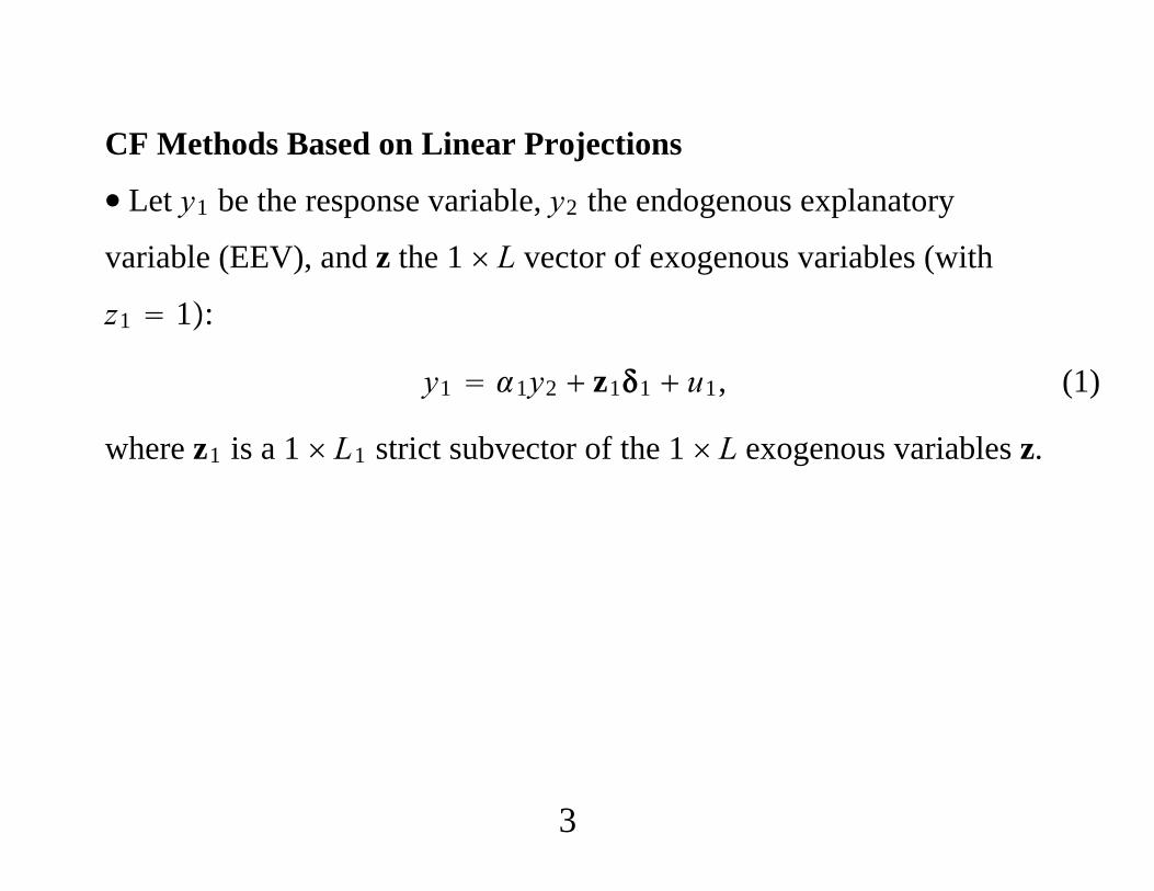
CF Methods Based on Linear Projections

∙ Let y1 be the response variable, y2 the endogenous explanatory

variable (EEV), and z the 1 L vector of exogenous variables (with

z1 1:

y1 1y2 z11 u1, (1)

where z1 is a 1 L1 strict subvector of the 1 L exogenous variables z.

3

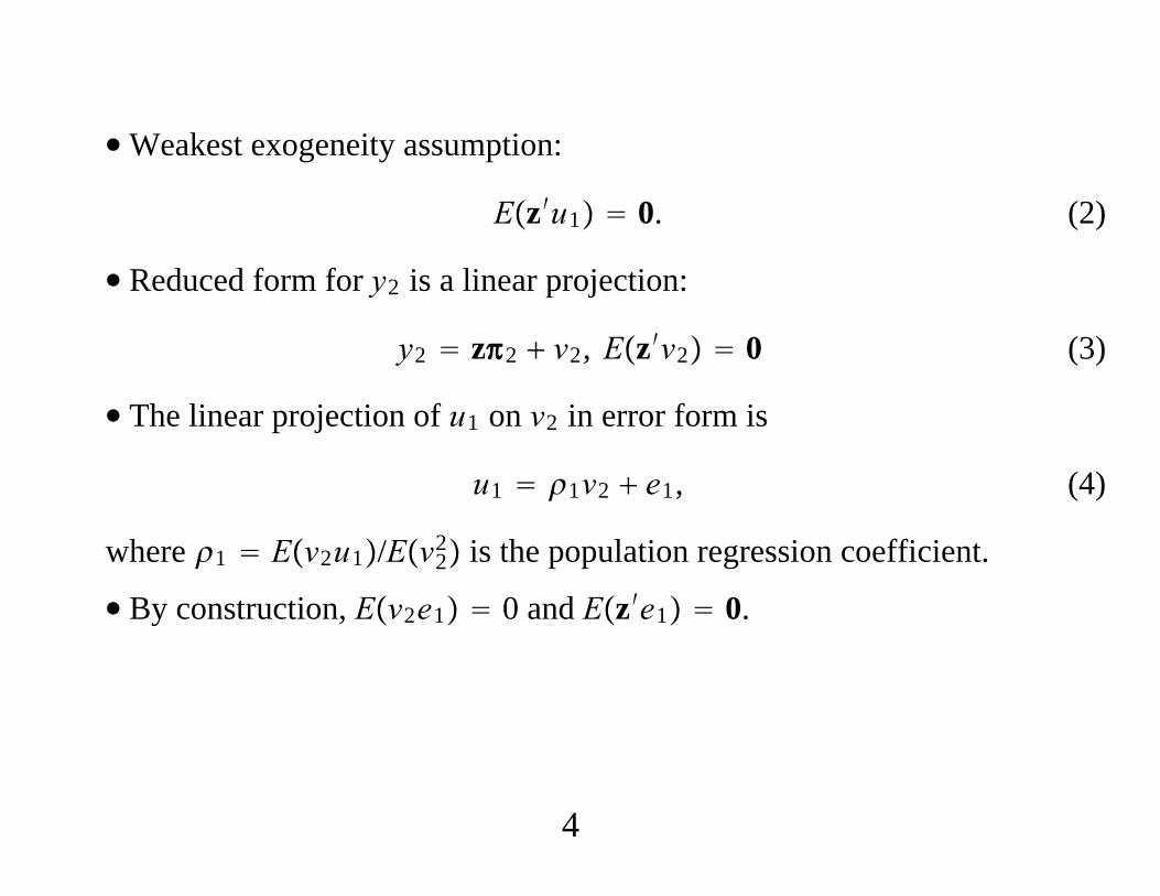
∙Weakest exogeneity assumption:

Ez′u1 0. (2)

∙ Reduced form for y2 is a linear projection:

y2 z2 v2, Ez′v2 0 (3)

∙ The linear projection of u1 on v2 in error form is

u1 1v2 e1, (4)

where 1 Ev2u1/Ev22 is the population regression coefficient.

∙ By construction, Ev2e1 0 and Ez′e1 0.

4

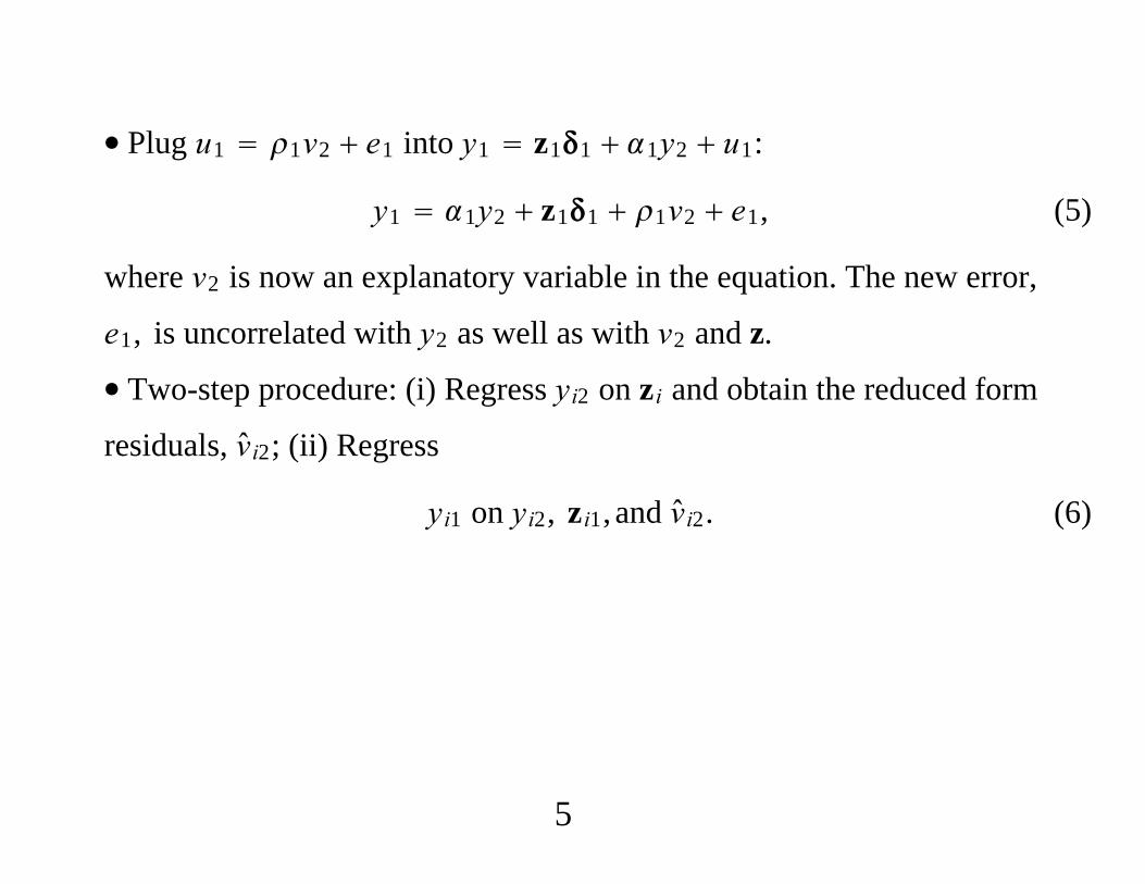
∙ Plug u1 1v2 e1 into y1 z11 1y2 u1:

y1 1y2 z11 1v2 e1, (5)

where v2 is now an explanatory variable in the equation. The new error,

e1, is uncorrelated with y2 as well as with v2 and z.

∙ Two-step procedure: (i) Regress yi2 on zi and obtain the reduced form

residuals, vi2; (ii) Regress

yi1 on yi2, zi1, and vi2. (6)

5

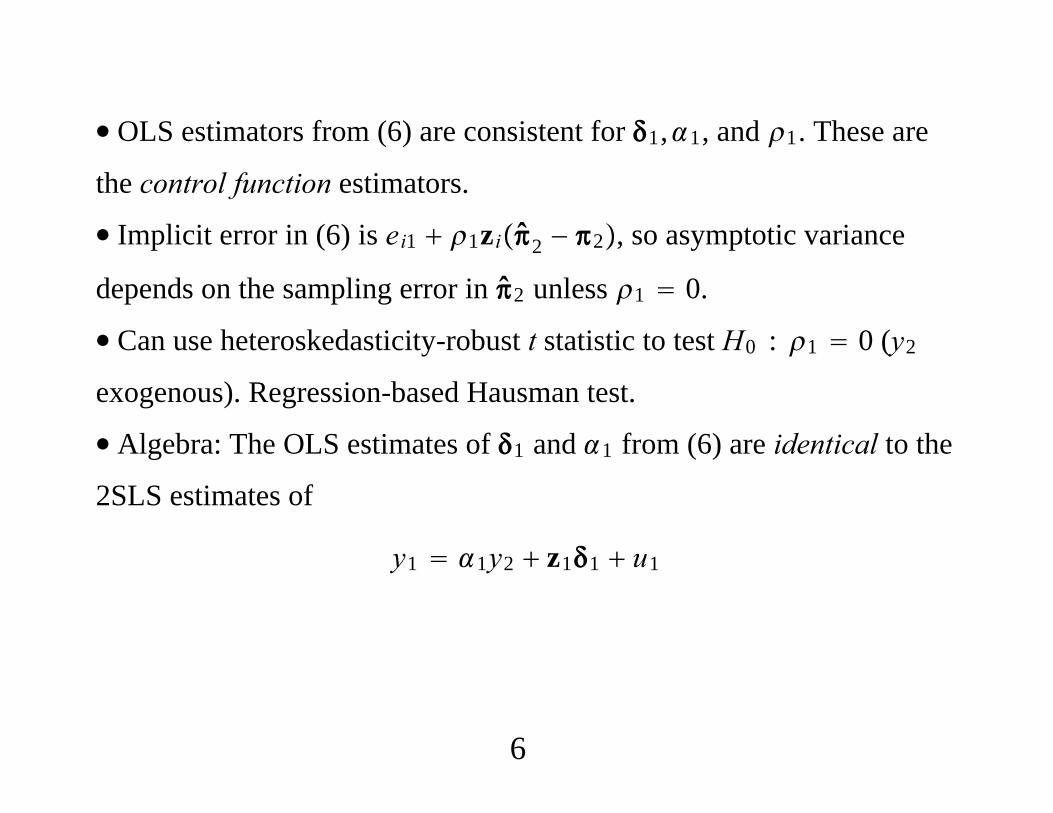
∙ OLS estimators from (6) are consistent for 1,1, and 1. These are

the control function estimators.

∙ Implicit error in (6) is ei1 1zi2 − 2, so asymptotic variance

depends on the sampling error in 2 unless 1 0.

∙ Can use heteroskedasticity-robust t statistic to test H0 : 1 0 (y2

exogenous). Regression-based Hausman test.

∙ Algebra: The OLS estimates of 1 and 1 from (6) are identical to the

2SLS estimates of

y1 1y2 z11 u1

6

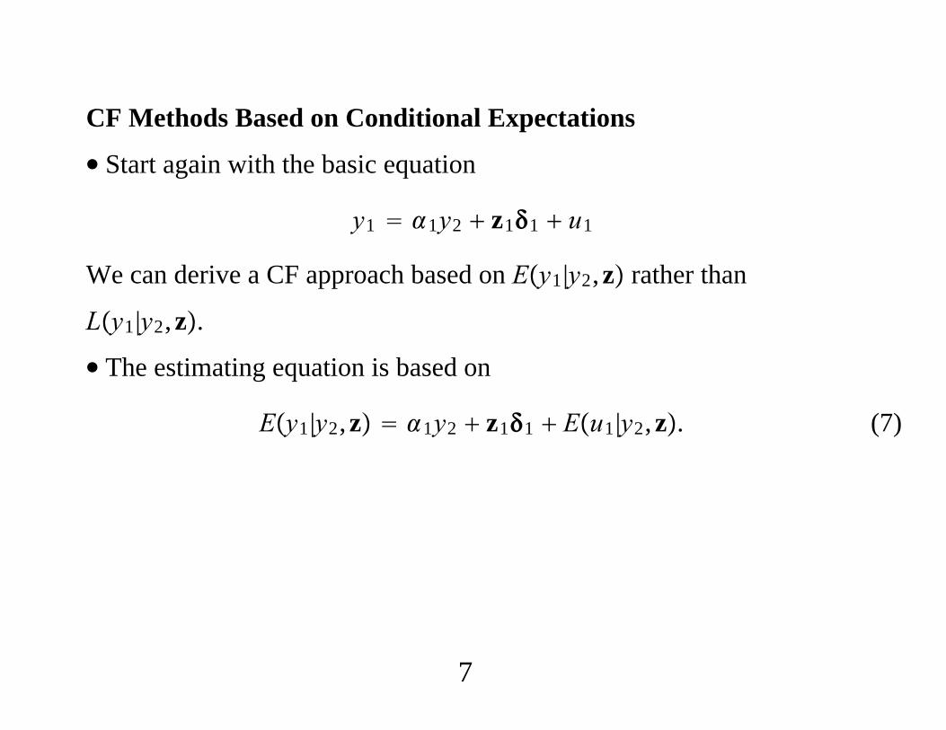
CF Methods Based on Conditional Expectations

∙ Start again with the basic equation

y1 1y2 z11 u1

We can derive a CF approach based on Ey1|y2,z rather than

Ly1|y2,z.

∙ The estimating equation is based on

Ey1|y2,z 1y2 z11 Eu1|y2,z. (7)

7

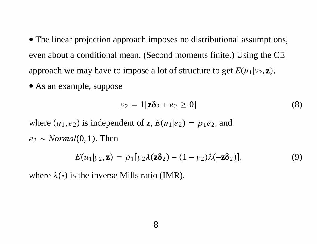
∙ The linear projection approach imposes no distributional assumptions,

even about a conditional mean. (Second moments finite.) Using the CE

approach we may have to impose a lot of structure to get Eu1|y2,z.

∙ As an example, suppose

y2 1z2 e2 ≥ 0 (8)

where u1,e2 is independent of z, Eu1|e2 1e2, and

e2 Normal0, 1. Then

Eu1|y2,z 1y2z2 − 1 − y2−z2, (9)

where is the inverse Mills ratio (IMR).

8

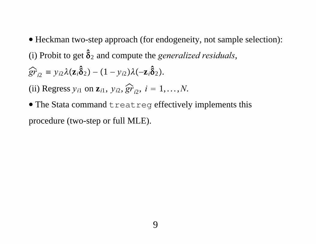
∙ Heckman two-step approach (for endogeneity, not sample selection):

(i) Probit to get 2 and compute the generalized residuals,

gri2 ≡ yi2zi2 − 1 − yi2−zi2.

(ii) Regress yi1 on zi1, yi2, gri2, i 1, . . . ,N.

∙ The Stata command treatreg effectively implements this

procedure (two-step or full MLE).

9

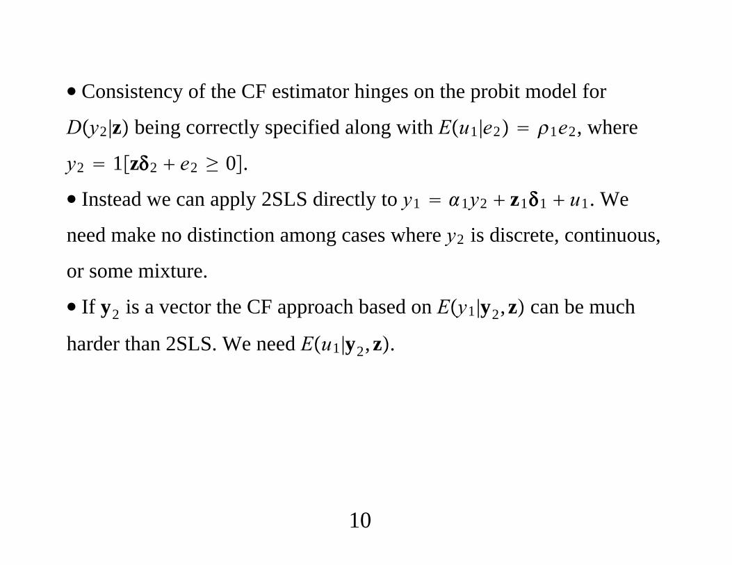
∙ Consistency of the CF estimator hinges on the probit model for

Dy2|z being correctly specified along with Eu1|e2 1e2, where

y2 1z2 e2 ≥ 0.

∙ Instead we can apply 2SLS directly to y1 1y2 z11 u1. We

need make no distinction among cases where y2 is discrete, continuous,

or some mixture.

∙ If y2 is a vector the CF approach based on Ey1|y2,z can be much

harder than 2SLS. We need Eu1|y2,z.

10

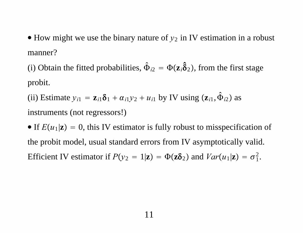
∙ How might we use the binary nature of y2 in IV estimation in a robust

manner?

(i) Obtain the fitted probabilities, i2 zi2, from the first stage

probit.

(ii) Estimate yi1 zi11 i1y2 ui1 by IV using zi1, i2 as

instruments (not regressors!)

∙ If Eu1|z 0, this IV estimator is fully robust to misspecification of

the probit model, usual standard errors from IV asymptotically valid.

Efficient IV estimator if Py2 1|z z2 and Varu1|z 12.

11

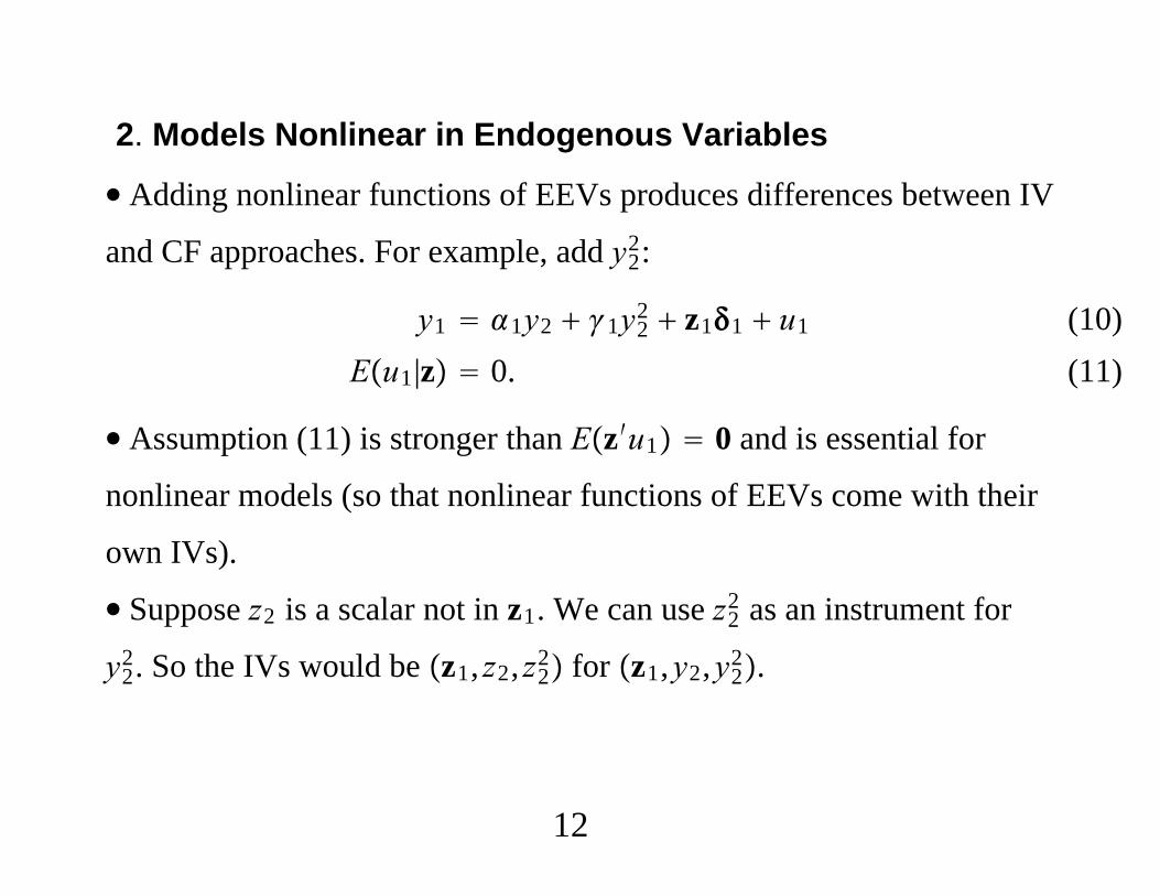
2. Models Nonlinear in Endogenous Variables

∙ Adding nonlinear functions of EEVs produces differences between IV

and CF approaches. For example, add y22:

y1 1y2 1y22 z11 u1

Eu1|z 0. (10) (11)

∙ Assumption (11) is stronger than Ez′u1 0 and is essential for

nonlinear models (so that nonlinear functions of EEVs come with their

own IVs).

∙ Suppose z2 is a scalar not in z1. We can use z22 as an instrument for

y22. So the IVs would be z1, z2, z2

2 for z1,y2,y22.

12

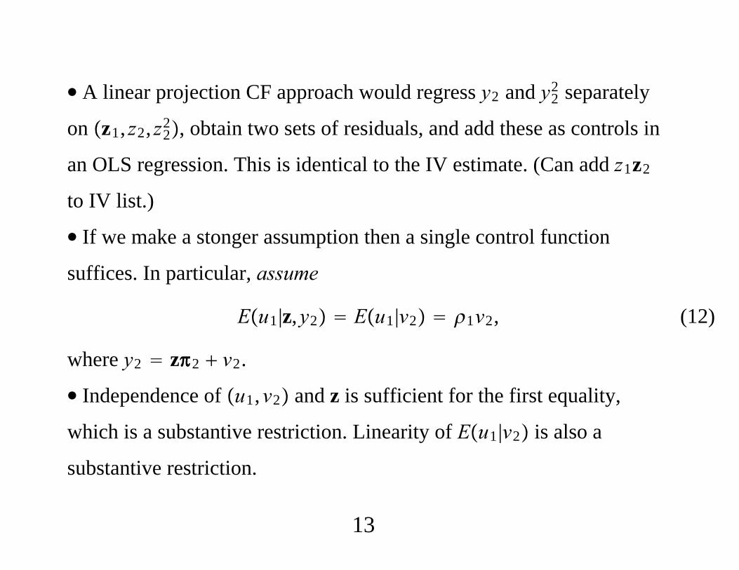
∙ A linear projection CF approach would regress y2 and y22 separately

on z1, z2, z22, obtain two sets of residuals, and add these as controls in

an OLS regression. This is identical to the IV estimate. (Can add z1z2

to IV list.)

∙ If we make a stonger assumption then a single control function

suffices. In particular, assume

Eu1|z,y2 Eu1|v2 1v2, (12)

where y2 z2 v2.

∙ Independence of u1,v2 and z is sufficient for the first equality,

which is a substantive restriction. Linearity of Eu1|v2 is also a

substantive restriction.

13

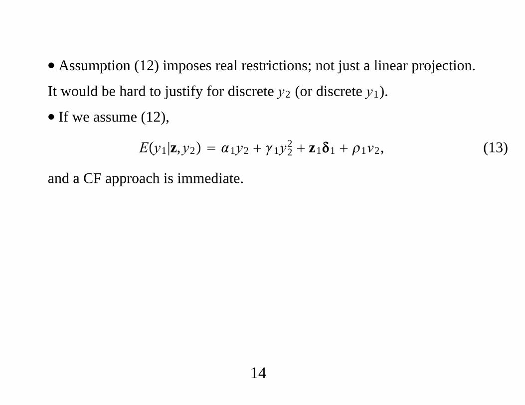
∙ Assumption (12) imposes real restrictions; not just a linear projection.

It would be hard to justify for discrete y2 (or discrete y1).

∙ If we assume (12),

Ey1|z,y2 1y2 1y22 z11 1v2, (13)

and a CF approach is immediate.

14

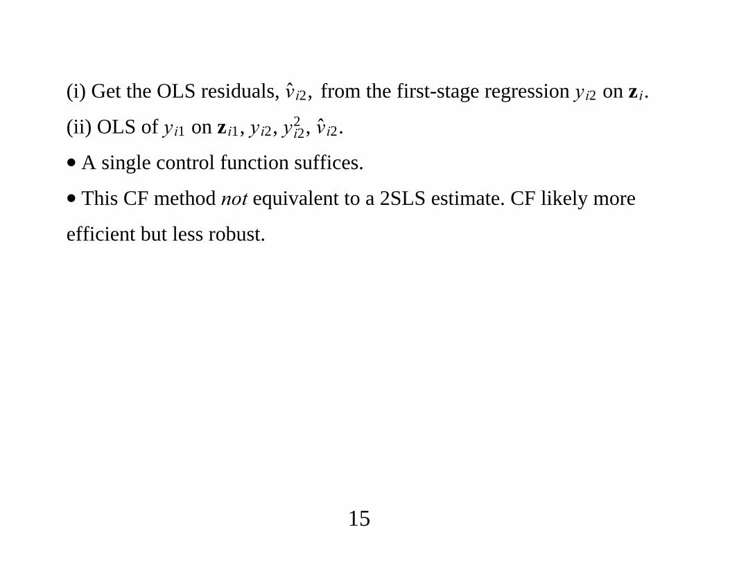
(i) Get the OLS residuals, vi2, from the first-stage regression yi2 on zi.

(ii) OLS of yi1 on zi1, yi2, yi22 , vi2.

∙ A single control function suffices.

∙ This CF method not equivalent to a 2SLS estimate. CF likely more

efficient but less robust.

15

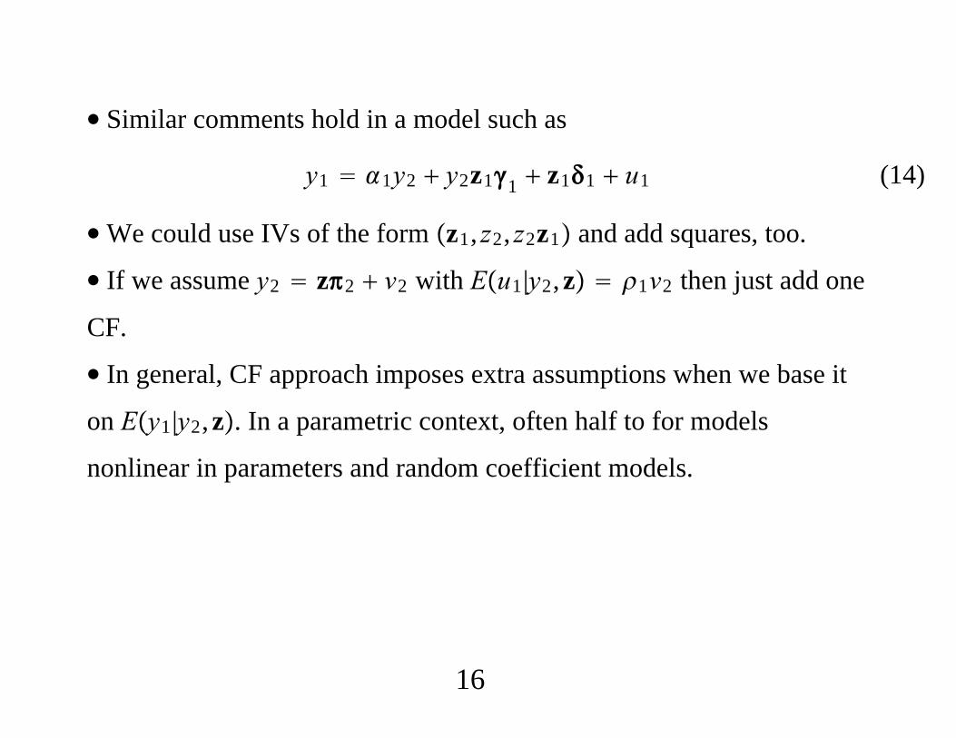
∙ Similar comments hold in a model such as

y1 1y2 y2z11 z11 u1 (14)

∙We could use IVs of the form z1, z2, z2z1 and add squares, too.

∙ If we assume y2 z2 v2 with Eu1|y2,z 1v2 then just add one

CF.

∙ In general, CF approach imposes extra assumptions when we base it

on Ey1|y2,z. In a parametric context, often half to for models

nonlinear in parameters and random coefficient models.

16

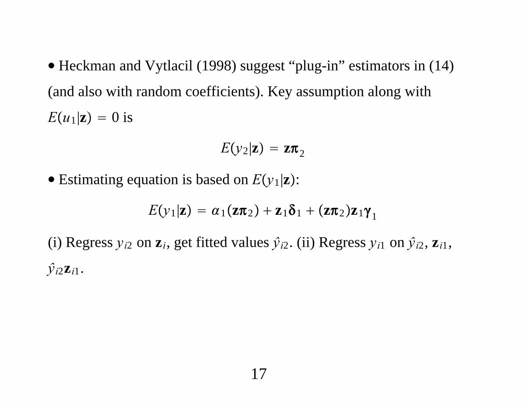
∙ Heckman and Vytlacil (1998) suggest “plug-in” estimators in (14)

(and also with random coefficients). Key assumption along with

Eu1|z 0 is

Ey2|z z2

∙ Estimating equation is based on Ey1|z:

Ey1|z 1z2 z11 z2z11

(i) Regress yi2 on zi, get fitted values ŷi2. (ii) Regress yi1 on ŷi2, zi1,

ŷi2zi1.

17

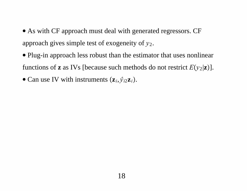
∙ As with CF approach must deal with generated regressors. CF

approach gives simple test of exogeneity of y2.

∙ Plug-in approach less robust than the estimator that uses nonlinear

functions of z as IVs [because such methods do not restrict Ey2|z].

∙ Can use IV with instruments zi,ŷi2zi.

18

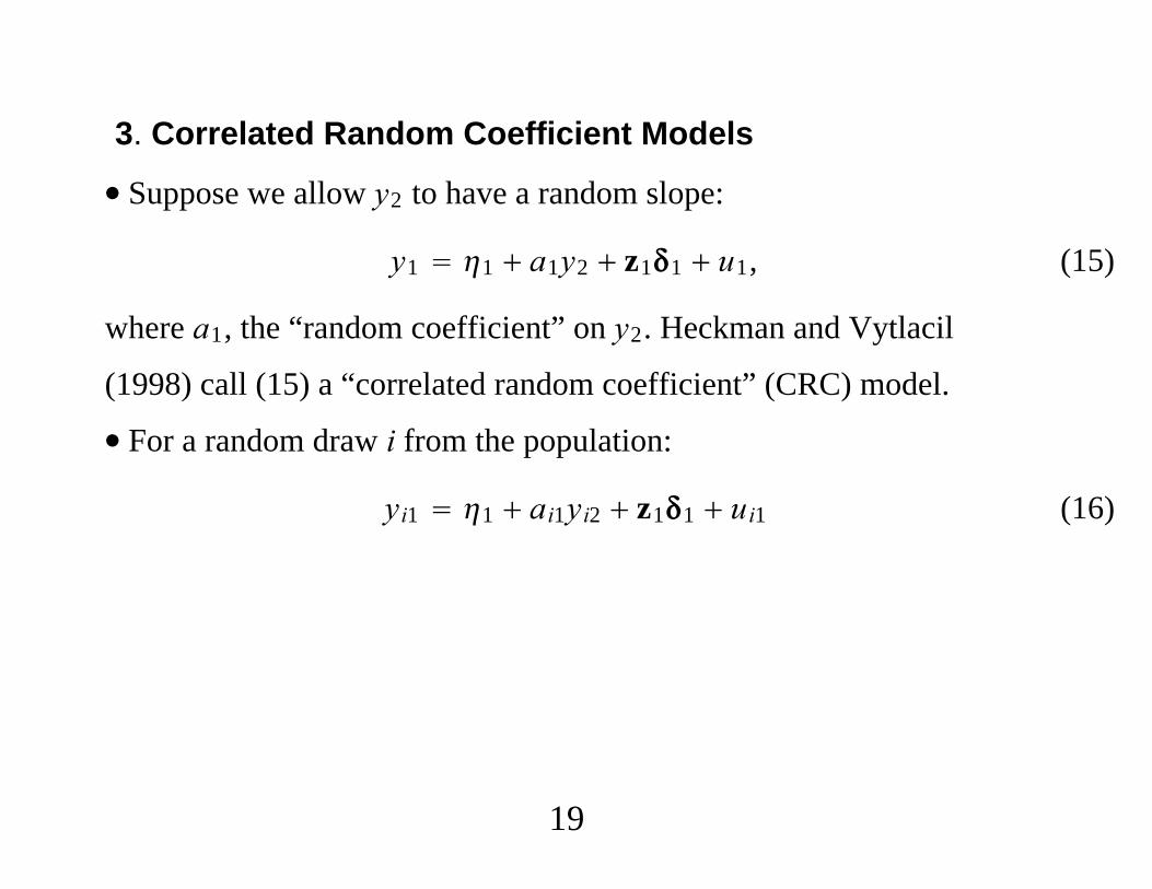
3. Correlated Random Coefficient Models

∙ Suppose we allow y2 to have a random slope:

y1 1 a1y2 z11 u1, (15)

where a1, the “random coefficient” on y2. Heckman and Vytlacil

(1998) call (15) a “correlated random coefficient” (CRC) model.

∙ For a random draw i from the population:

yi1 1 ai1yi2 z11 ui1 (16)

19

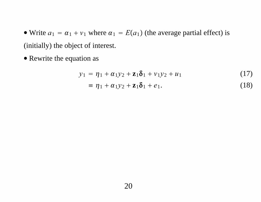
∙Write a1 1 v1 where 1 Ea1 (the average partial effect) is

(initially) the object of interest.

∙ Rewrite the equation as

y1 1 1y2 z11 v1y2 u1

≡ 1 1y2 z11 e1. (17) (18)

20

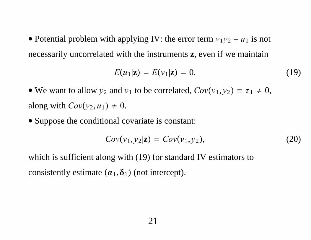
∙ Potential problem with applying IV: the error term v1y2 u1 is not

necessarily uncorrelated with the instruments z, even if we maintain

Eu1|z Ev1|z 0. (19)

∙We want to allow y2 and v1 to be correlated, Covv1,y2 ≡ 1 ≠ 0,

along with Covy2,u1 ≠ 0.

∙ Suppose the conditional covariate is constant:

Covv1,y2|z Covv1,y2, (20)

which is sufficient along with (19) for standard IV estimators to

consistently estimate 1,1 (not intercept).

21

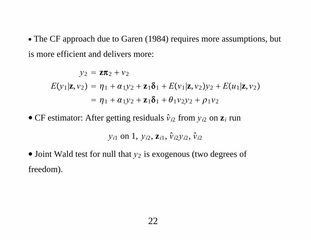
∙ The CF approach due to Garen (1984) requires more assumptions, but

is more efficient and delivers more:

y2 z2 v2

Ey1|z,v2 1 1y2 z11 Ev1|z,v2y2 Eu1|z,v2

1 1y2 z11 1v2y2 1v2

∙ CF estimator: After getting residuals vi2 from yi2 on zi run

yi1 on 1, yi2, zi1, vi2yi2, vi2

∙ Joint Wald test for null that y2 is exogenous (two degrees of

freedom).

22

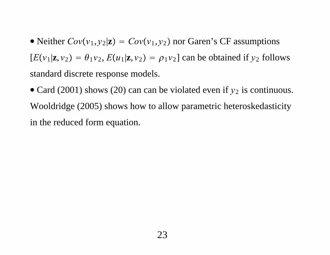
∙ Neither Covv1,y2|z Covv1,y2 nor Garen’s CF assumptions

[Ev1|z,v2 1v2, Eu1|z,v2 1v2] can be obtained if y2 follows

standard discrete response models.

∙ Card (2001) shows (20) can can be violated even if y2 is continuous.

Wooldridge (2005) shows how to allow parametric heteroskedasticity

in the reduced form equation.

23

4. Endogenous Switching

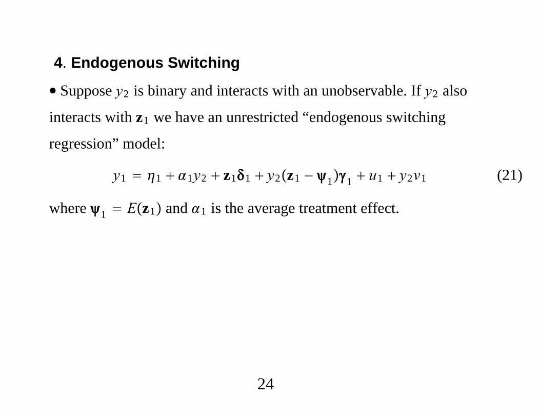
∙ Suppose y2 is binary and interacts with an unobservable. If y2 also

interacts with z1 we have an unrestricted “endogenous switching

regression” model:

y1 1 1y2 z11 y2z1 − 11 u1 y2v1 (21)

where 1 Ez1 and 1 is the average treatment effect.

24

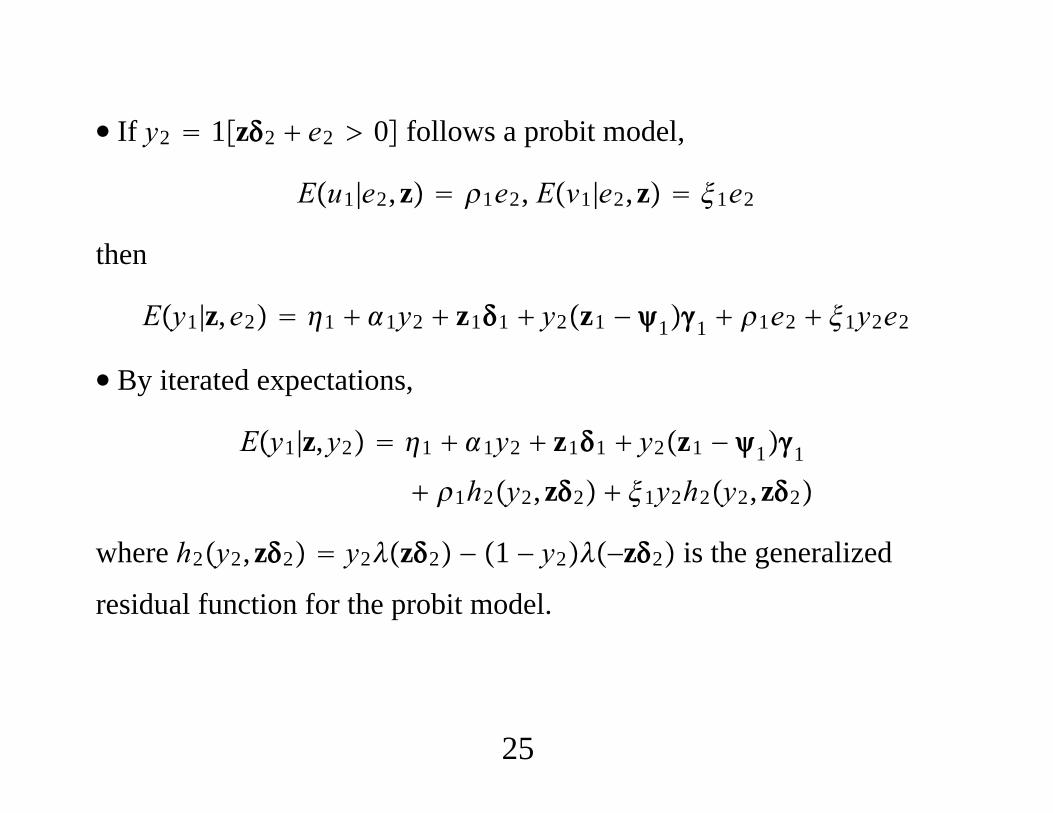
∙ If y2 1z2 e2 0 follows a probit model,

Eu1|e2,z 1e2, Ev1|e2,z 1e2

then

Ey1|z,e2 1 1y2 z11 y2z1 − 11 1e2 1y2e2

∙ By iterated expectations,

Ey1|z,y2 1 1y2 z11 y2z1 − 11

1h2y2,z2 1y2h2y2,z2

where h2y2,z2 y2z2 − 1 − y2−z2 is the generalized

residual function for the probit model.

25

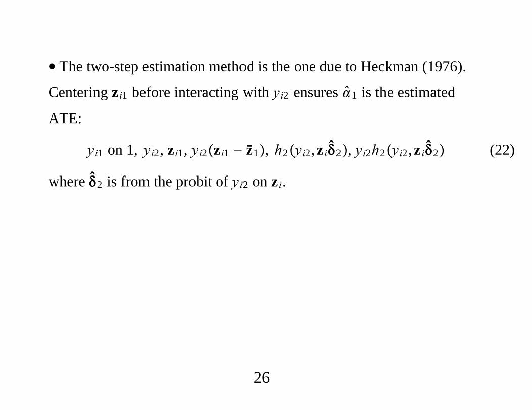
∙ The two-step estimation method is the one due to Heckman (1976).

Centering zi1 before interacting with yi2 ensures 1 is the estimated

ATE:

yi1 on 1, yi2, zi1, yi2zi1 − z1, h2yi2,zi2, yi2h2yi2,zi2 (22)

where 2 is from the probit of yi2 on zi.

26

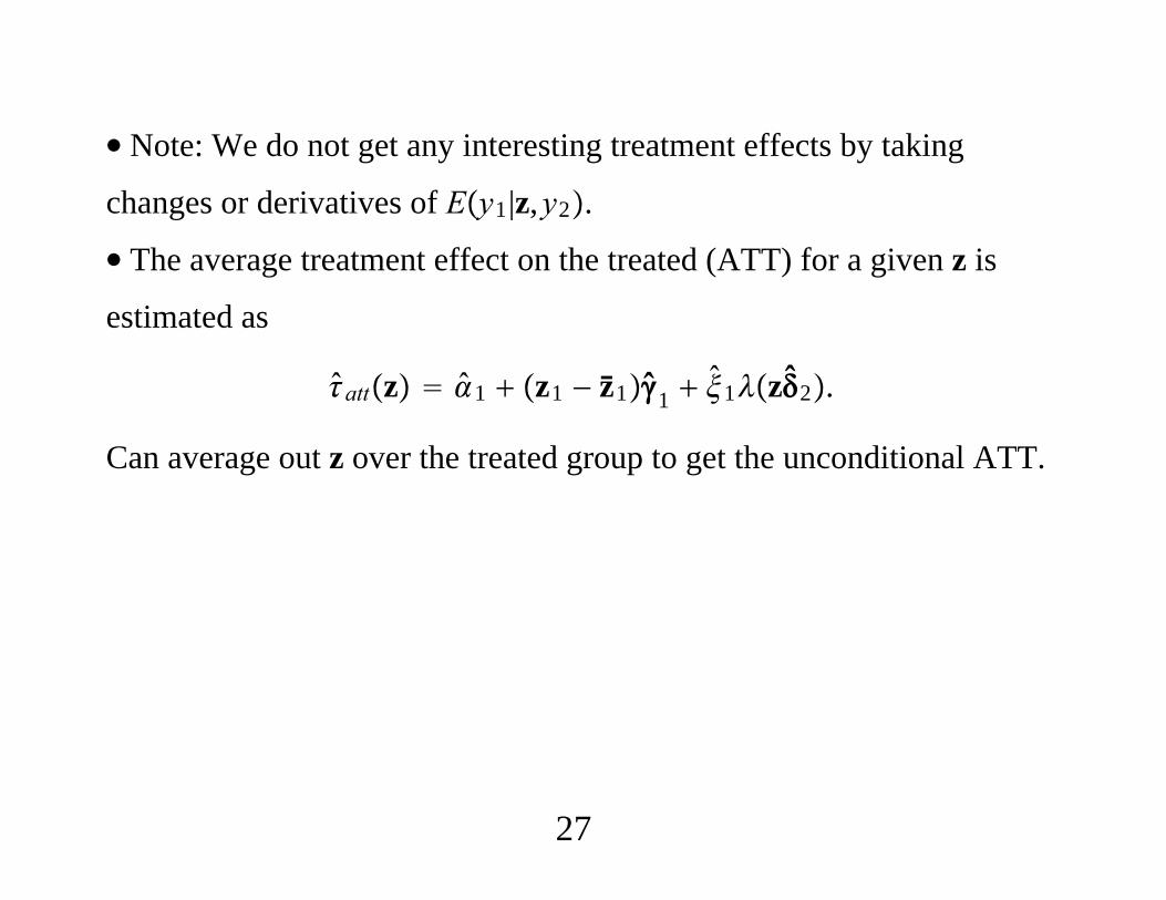
∙ Note: We do not get any interesting treatment effects by taking

changes or derivatives of Ey1|z,y2.

∙ The average treatment effect on the treated (ATT) for a given z is

estimated as

attz 1 z1 − z11 1z2.

Can average out z over the treated group to get the unconditional ATT.

27

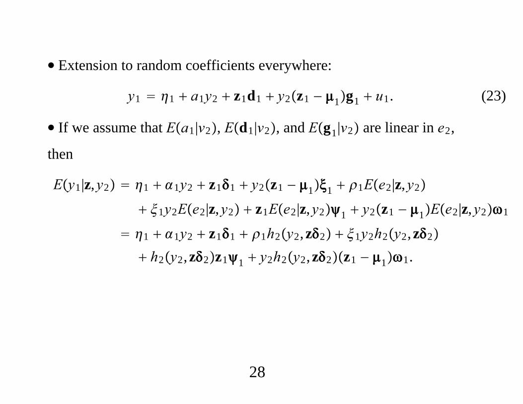
∙ Extension to random coefficients everywhere:

y1 1 a1y2 z1d1 y2z1 − 1g1 u1. (23)

∙ If we assume that Ea1|v2, Ed1|v2, and Eg1|v2 are linear in e2,

then

Ey1|z,y2 1 1y2 z11 y2z1 − 11 1Ee2|z,y2

1y2Ee2|z,y2 z1Ee2|z,y21 y2z1 − 1Ee2|z,y21

1 1y2 z11 1h2y2,z2 1y2h2y2,z2

h2y2,z2z11 y2h2y2,z2z1 − 11.

28

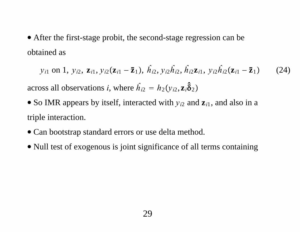
∙ After the first-stage probit, the second-stage regression can be

obtained as

yi1 on 1, yi2, zi1, yi2zi1 − z1, ĥi2, yi2ĥi2, ĥi2zi1, yi2ĥi2zi1 − z1 (24)

across all observations i, where ĥi2 h2yi2,zi2

∙ So IMR appears by itself, interacted with yi2 and zi1, and also in a

triple interaction.

∙ Can bootstrap standard errors or use delta method.

∙ Null test of exogenous is joint significance of all terms containing

29

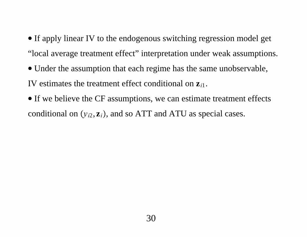
∙ If apply linear IV to the endogenous switching regression model get

“local average treatment effect” interpretation under weak assumptions.

∙ Under the assumption that each regime has the same unobservable,

IV estimates the treatment effect conditional on zi1.

∙ If we believe the CF assumptions, we can estimate treatment effects

conditional on yi2,zi, and so ATT and ATU as special cases.

30

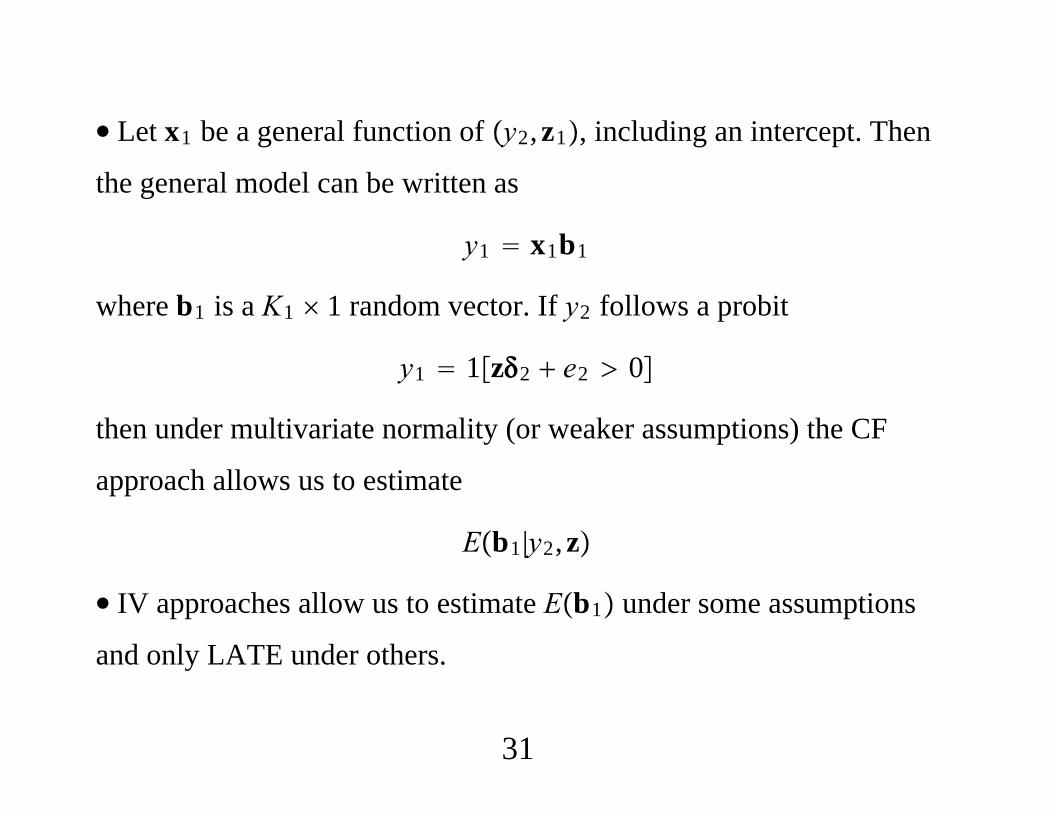
∙ Let x1 be a general function of y2,z1, including an intercept. Then

the general model can be written as

y1 x1b1

where b1 is a K1 1 random vector. If y2 follows a probit

y1 1z2 e2 0

then under multivariate normality (or weaker assumptions) the CF

approach allows us to estimate

Eb1|y2,z

∙ IV approaches allow us to estimate Eb1 under some assumptions

and only LATE under others.

31

5. Random Coefficients in Reduced Forms

∙ Random coefficients in reduced forms ruled out in Blundell and

Powell (2003) and Imbens and Newey (2006).

∙ Hoderlein, Nesheim, and Simoni (2012) show cannot generally get

point identification, even in simple model.

∙ Of interest because the reaction of individual units to changes in the

instrument may differ in unobserved ways.

∙ Under enough assumptions can obtain new CF methods in linear

models that allow for slope heterogeneity everywhere.

32

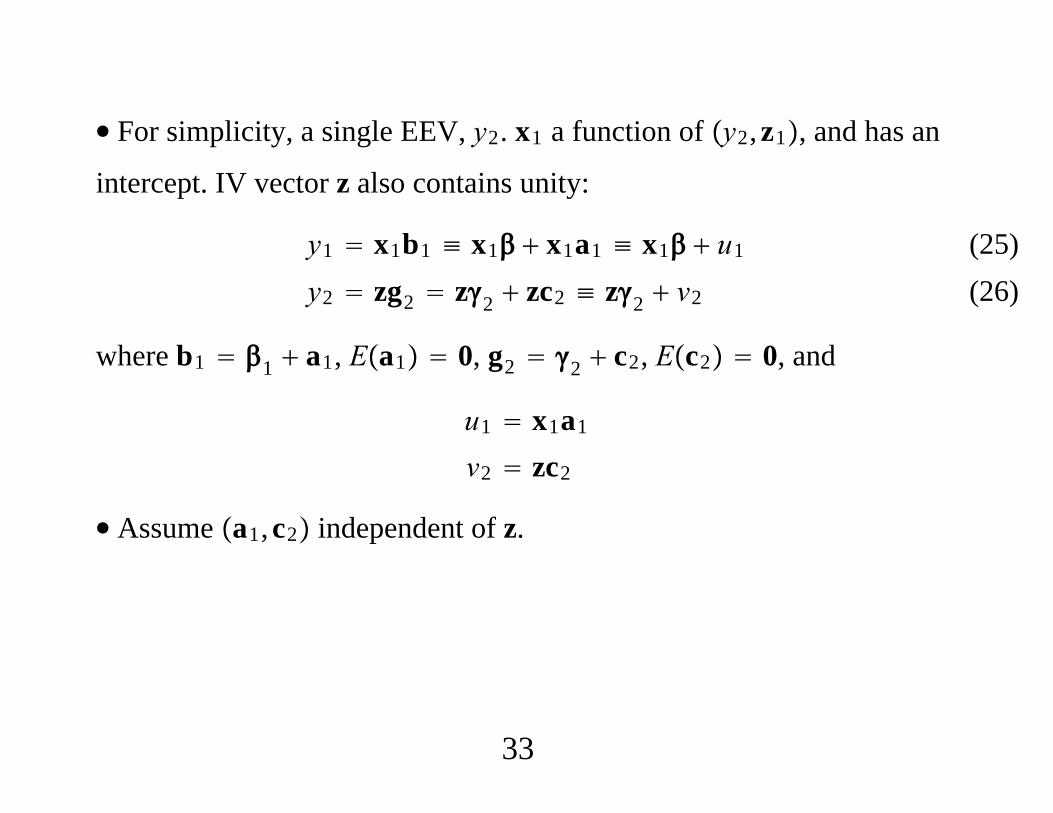
∙ For simplicity, a single EEV, y2. x1 a function of y2,z1, and has an

intercept. IV vector z also contains unity:

y1 x1b1 ≡ x1 x1a1 ≡ x1 u1

y2 zg2 z2 zc2 ≡ z2 v2

(25) (26)

where b1 1 a1, Ea1 0, g2 2 c2, Ec2 0, and

u1 x1a1

v2 zc2

∙ Assume a1,c2 independent of z.

33

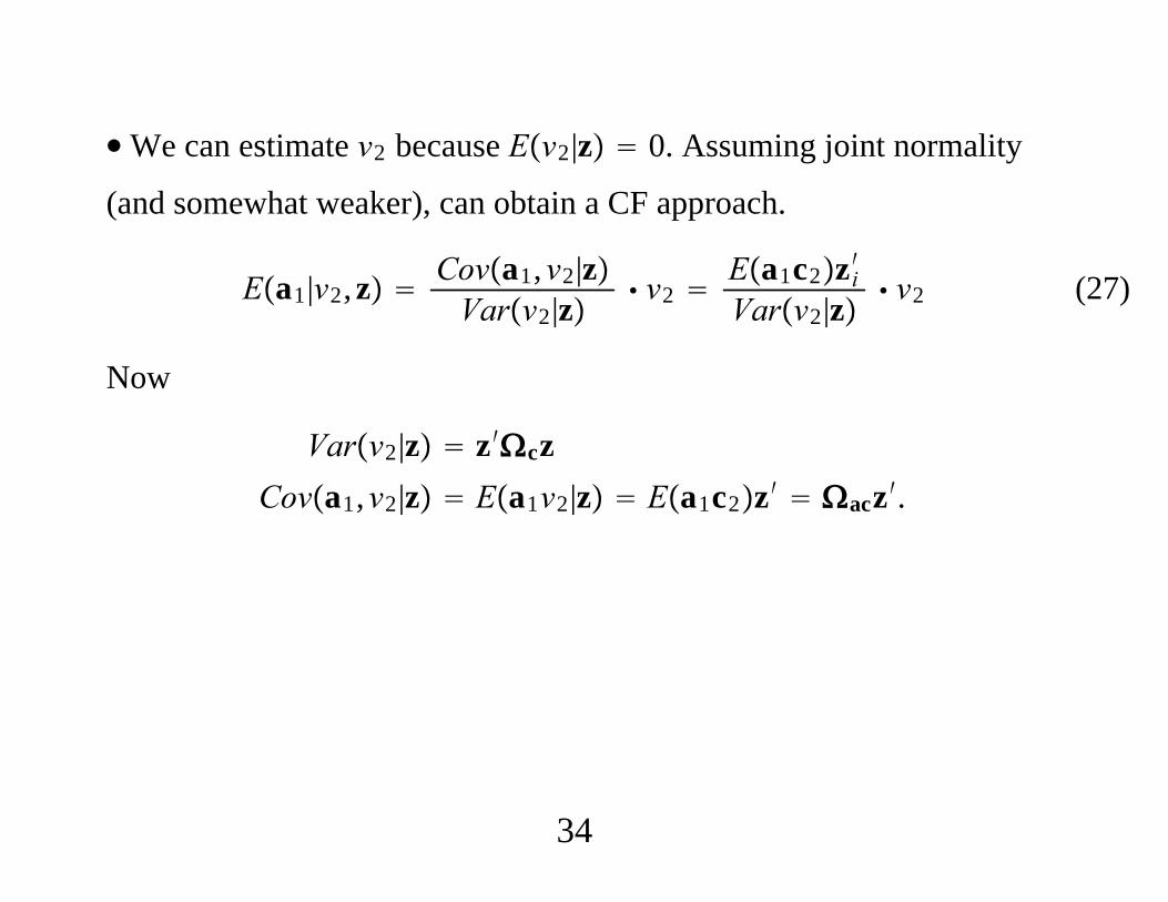
∙We can estimate v2 because Ev2|z 0. Assuming joint normality

(and somewhat weaker), can obtain a CF approach.

Ea1|v2,z Cova1,v2|zVarv2|z v2

Ea1c2zi′Varv2|z v2 (27)

Now

Varv2|z z′czCova1,v2|z Ea1v2|z Ea1c2z′ acz′.

34

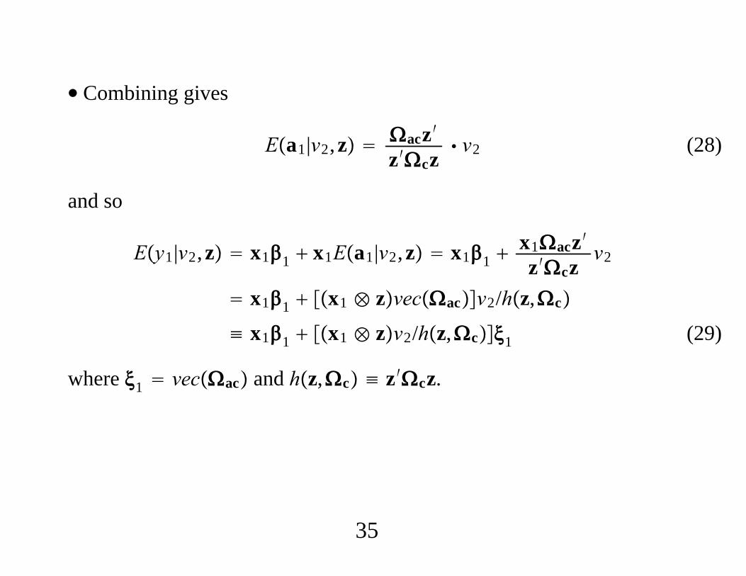
∙ Combining gives

Ea1|v2,z acz′z′cz

v2 (28)

and so

Ey1|v2,z x11 x1Ea1|v2,z x11 x1acz′z′cz

v2

x11 x1 ⊗ zvecacv2/hz,c

≡ x11 x1 ⊗ zv2/hz,c1 (29)

where 1 vecac and hz,c ≡ z′cz.

35

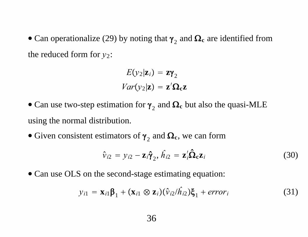
∙ Can operationalize (29) by noting that 2 and c are identified from

the reduced form for y2:

Ey2|zi z2

Vary2|z z′cz

∙ Can use two-step estimation for 2 and c but also the quasi-MLE

using the normal distribution.

∙ Given consistent estimators of 2 and c, we can form

vi2 yi2 − zi2, ĥi2 zi′czi (30)

∙ Can use OLS on the second-stage estimating equation:

yi1 xi11 xi1 ⊗ zivi2/ĥi21 errori (31)

36

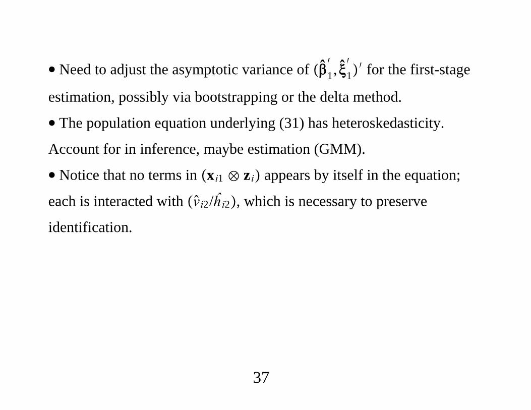
∙ Need to adjust the asymptotic variance of 1′ , 1

′′ for the first-stage

estimation, possibly via bootstrapping or the delta method.

∙ The population equation underlying (31) has heteroskedasticity.

Account for in inference, maybe estimation (GMM).

∙ Notice that no terms in xi1 ⊗ zi appears by itself in the equation;

each is interacted with vi2/ĥi2, which is necessary to preserve

identification.

37