CONTRIBUTIONS TO THE TRUNCATED VON MISES …cig.fi.upm.es/thesis/master/Contributions to the truncated von... · CONTRIBUTIONS TO THE TRUNCATED VON MISES ... dos de este trabajo para

ESCUELA TECNICA SUPERIOR DE INGENIEROSINFORMATICOS

UNIVERSIDAD POLITECNICA DE MADRID

MASTER’S THESIS IN ARTIFICIAL

INTELLIGENCE

CONTRIBUTIONS TO THETRUNCATED VON MISESDISTRIBUTION FOR THE

UNIVARIATE AND BIVARIATECASE

AUTHOR : Pablo Fernandez GonzalezSUPERVISORS : Concha Bielza Lozoya

Pedro Larranaga Mugica

Jun, 2014

ii

Acknowledgments

To my master thesis supervisors Concha Bielza and Pedro Larranaga, for their adviceand guidance through the process of attaining this work to completion.

iii

iv

Resumen

En esta tesis describimos y caracterizamos la distribucion von Mises truncada en suforma univariante y bivariante y proveemos de desarrollos adicionales que en con-junto especifican la definicion y aplicaciones de esta distribucion de probabilidad.Establecemos esta distribucion a un nivel de desarrollo suficiente para que pueda seraplicada en problemas de modelado y simulacion que pudieran aparecer en cualquiercampo del conocimiento siendo explorado por el ser humano. Aplicamos los resulta-dos de este trabajo para modelar y estudiar la distribucion de angulos dendrıticos enneuronas piramidales de la capa III del cortex cerebral en ratones, como un ejemplode lo que puede conseguirse utilizando la metodologa desarrollada.

v

vi

Abstract

In this thesis we describe and characterize the truncated von Mises distribution inits univariate and bivariate form and we provide different additional developmentsthat in conjunction will specify the definition and applications of this probabilitydistribution. We set this distribution to a sufficient level of development for it to beapplied to modeling and simulation problems that may arise in any area of knowledgeunder human exploration. We apply the findings of this work to model and study thedistribution of dendritic angles in cerebral cortex layer III mice pyramidal neuronsas an example of what can be achieved by analyzing the data with the developedmethodology.

vii

viii

List of Figures

1.1 In radians, the incorrect distance of (2π)79

that the classical mean

computed (red) compared to the correct solution of (2π)29

(blue). . . . 3

1.2 The incorrectly calculated mean of 0◦, 30◦ and 360◦ using standardstatistics (red) compared to the correct solution (blue). . . . . . . . . 4

1.3 Both circular Cartesian and complex number coordinates approachesto reference the angle θ = 3

4π in the circle once initial direction (coun-

terclockwise) and reference angle (0 degrees) have been chosen. . . . . 5

1.4 For angles 0◦, 30◦, 55◦, 78◦, 145◦ and 330◦, the correctly calculatedmean and the mean resultant length. The calculated values were:θ = 54◦26′49.2′′ and R = 0.5828. . . . . . . . . . . . . . . . . . . . . . 9

2.1 Example of different von Mises density functions with varying µ, κparameters. . . . . . . . . . . . . . . . . . . . . . . . . . . . . . . . . 13

2.2 The von Mises distribution functions of the previously shown vonMises density distributions. . . . . . . . . . . . . . . . . . . . . . . . 14

3.1 Several truncated von Mises distributions with varying parametersthat include all cases. Symmetrical truncation w.r.t. the mean (red),strictly increasing function (blue), strictly decreasing function (green),symmetrical antimode truncation (black), maximum and minimumincluded truncation (yellow). . . . . . . . . . . . . . . . . . . . . . . 25

3.2 The distribution functions of all the truncated distributions describedin Figure 3.1. Notice how the functions do not increase outside thetruncation limits. . . . . . . . . . . . . . . . . . . . . . . . . . . . . . 26

3.3 I0(x) evaluated in the interval [0, 2π]. . . . . . . . . . . . . . . . . . . 28

3.4 Example of the bi-dimensional von Mises distribution with parame-ters λ = 1, µ1 = 2, µ2 = 4, κ1 = 3, κ2 = 2, a1 = 0, b1 = 3.8, a2 =2, b2 = 5. . . . . . . . . . . . . . . . . . . . . . . . . . . . . . . . . . . 45

3.5 Same distribution as in Figure 3.4 although projected, appreciatingthe truncation parameters from two axis perspectives. . . . . . . . . . 46

ix

x LIST OF FIGURES

3.6 Several truncated marginals showing unimodality (red) with param-eters λ = 5, µ1 = π, µ2 = 0, κ1 = 1, κ2 = 4, a1 = 0, b1 = 2π, a2 =π − 0.2, b2 = 2π, two equal maxima (blue) with parameters λ =5, µ1 = π, µ2 = 0, κ1 = 1, κ2 = 4, a1 = 0, b1 = 2π, a2 = 0, b2 = 2π,truncated unimodality (green) with parameters λ = 1, µ1 = 4, µ2 =2, κ1 = 3, κ2 = 4, a1 = 0, b1 = 5, a2 = 2, b2 = 2π and 2 distinct max-ima (black) with parameters λ = 10, µ1 = 6, µ2 = 1, κ1 = 0.3, κ2 =6, a1 = 0, b1 = 2π, a2 = 0, b2 = 5 respectively. . . . . . . . . . . . . . . 54

3.7 Marginal truncated von Mises with parameters λ = 5, µ1 = π, µ2 = 4,κ1 = 2, κ2 = 4 and b2 = 5. The difference between each of themis given by variation on the a2 truncation parameter. For a2 = 2(black), we have cos(b2 − µ2) > cos(a2 − µ2) and therefore a maxi-mum (the global maximum) is found in the interval [π

2, π]. For a2 = 3

(blue), cos(b2 − µ2) = cos(a2 − µ2) where the distribution presentstwo global maxima. For a2 = 3.2, cos(b2 − µ2) < cos(a2 − µ2) andfumtvM(θ1′) presents two critical points in the interval [π

2, π]. For

a2 = 3.3565 (approximated value), cos(b2 − µ2) < cos(a2 − µ2) andfumtvM(θ1′) presents exactly one critical point in [π

2, π]. For a2 = 3.5,

cos(b2−µ2) < cos(a2−µ2) and fumtvM(θ1′) presents no critical point inthe interval [π

2, π] and therefore the distribution is unimodal. Lastly,

for a2 = 4 we fall into the most restrictive case of cos(b2 − µ2) <

cos(a2−µ2) where −∫ µ2a2f0v2′ (θ2;

π2)dθ2 ≤

∫ b2µ2f0v2′ (θ2;

π2)dθ2 (the pre-

vious cos(b2 − µ2) < cos(a2 − µ2) cases fell under the complementarycase, where the integral comparison did not verify the inequation) andmore specifically the case where a2, b2 ∈ [µ2, µ2 + π], which forces thedistribution to present a unimodal behavior regardless of the otherparameter values in the interval [π

2, π]. The progression followed by

the distribution under modifying the a2 parameter can be seen, un-der appearances, as an “area shifting” process where approaching µ2

displacing a truncation parameter carries with it as well a displace-ment of the area of the distribution towards that direction, leavingthe global maxima always in the π

2−interval including µ1 associated

with the truncation parameter whose circular distance to µ2 is higher.The “displacement” of a2 in this case seems to increase the value ofthe maxima in [π, 3

2π] and decrease the value of the maxima in [π

2, π]

in the bi-maximal case until the distribution becomes unimodal, andthen continue by decreasing the area under the monotonic curve. . . . 60

4.1 Graphical visualization of the organization of the dataset. . . . . . . . 65

4.2 Estimated truncated von Mises distribution for the entire dataset.This distribution corresponds to the parameter values of the 9th row(named “All”) in Table 4.1. . . . . . . . . . . . . . . . . . . . . . . . 66

LIST OF FIGURES xi

4.3 Estimated bivariate truncated von Mises distribution for the jointdata of the bifurcation levels 1 and 2. The parameter values of thisdistribution are those in the second column of Table 4.4 (named “Bif1-2”). . . . . . . . . . . . . . . . . . . . . . . . . . . . . . . . . . . . . . 70

4.4 Marginal distribution of the first component (Bifurcation 1) in thebivariate case for Bifurcation levels 1 and 2 shown in Figure 4.3. . . . 71

4.5 Marginal distribution of the second component (Bifurcation 2) in thebivariate case for Bifurcation levels 1 and 2 shown in Figure 4.3. . . . 71

xii LIST OF FIGURES

List of Tables

4.1 Parameter values of truncated von Mises distributions of each groupaccording to the brain area, and the whole dataset. . . . . . . . . . . 66

4.2 Estimated truncated von Mises distributions for the entire datasetseparated in 6 bifurcation levels. We can notice the emergence of apattern when examining the values of the µ parameter, that seem todecrease when increasing the level we look at. . . . . . . . . . . . . . 67

4.3 Estimated truncated von Mises distributions for the different brainareas and for the different bifurcation levels. We can notice how thedecreasing µ pattern is highly consistent appearing in every subgroupexcept for PrL and M1 in the fewer samples estimator (levels 4 and5, respectively). . . . . . . . . . . . . . . . . . . . . . . . . . . . . . 68

4.4 Estimated truncated bivariate von Mises distributions for pairs ofbifurcation levels from one to five in the whole dataset. We cannotice that the estimation seems to show tendency to independenceby a decreasing tendency in the λ parameter. Also, there exists adecreasing tendency shown by both means µ1, µ2 . . . . . . . . . . . 69

4.5 Estimated truncated bivariate von Mises distributions for pairs of bi-furcation levels from one to five in the M1 region. Here the decreasingtendency in the λ parameter is not followed by either Bif1-2 or by Bif2-3. 72

4.6 Estimated truncated bivariate von Mises distributions for pairs ofbifurcation levels from one to four in the M2 region. . . . . . . . . . . 72

4.7 Estimated truncated bivariate von Mises distributions for pairs ofbifurcation levels from one to four in the PrL region. . . . . . . . . . 73

4.8 Estimated truncated bivariate von Mises distributions for pairs ofbifurcation levels from one to five in the S1 region. . . . . . . . . . . 73

4.9 Estimated truncated bivariate von Mises distributions for pairs ofbifurcation levels from one to four in the S2 region. . . . . . . . . . . 74

4.10 Estimated truncated bivariate von Mises distributions for pairs ofbifurcation levels from one to four in the V1 region. . . . . . . . . . 74

4.11 Estimated truncated bivariate von Mises distributions for pairs ofbifurcation levels from one to four in the V2 region. . . . . . . . . . 75

xiii

xiv LIST OF TABLES

Contents

List of Figures ix

List of Tables xiii

1 Introduction 11.1 Scope, motivation and objectives of the present work . . . . . . . . . 11.2 Directional statistics . . . . . . . . . . . . . . . . . . . . . . . . . . . 2

1.2.1 Coordinate systems and the limitations of classical statistics . 3

2 The von Mises distribution 112.1 Definition . . . . . . . . . . . . . . . . . . . . . . . . . . . . . . . . . 122.2 Properties . . . . . . . . . . . . . . . . . . . . . . . . . . . . . . . . . 132.3 Maximum likelihood estimation . . . . . . . . . . . . . . . . . . . . . 152.4 Characteristic function . . . . . . . . . . . . . . . . . . . . . . . . . . 172.5 Moments . . . . . . . . . . . . . . . . . . . . . . . . . . . . . . . . . . 18

3 Truncated von Mises distribution 213.1 Truncated distribution . . . . . . . . . . . . . . . . . . . . . . . . . . 213.2 Definition . . . . . . . . . . . . . . . . . . . . . . . . . . . . . . . . . 223.3 Properties . . . . . . . . . . . . . . . . . . . . . . . . . . . . . . . . . 233.4 Bessel functions . . . . . . . . . . . . . . . . . . . . . . . . . . . . . . 26

3.4.1 Some results on the modified Bessel functions of the first kind 283.4.2 Calculating the indefinite integral of the unnormalized von

Mises function by means of its power series expansion . . . . . 313.5 Maximum likelihood estimation of the parameters . . . . . . . . . . . 363.6 Characteristic function . . . . . . . . . . . . . . . . . . . . . . . . . . 403.7 Moments . . . . . . . . . . . . . . . . . . . . . . . . . . . . . . . . . . 403.8 The bi-dimensional truncated von Mises distribution . . . . . . . . . 42

3.8.1 Definition . . . . . . . . . . . . . . . . . . . . . . . . . . . . . 433.8.2 Parameter estimation . . . . . . . . . . . . . . . . . . . . . . . 473.8.3 Conditional and marginal truncated von Mises distributions . 49

4 Application in Neuroscience 634.1 Data organization . . . . . . . . . . . . . . . . . . . . . . . . . . . . . 634.2 Unidimensional von Mises distribution fitting . . . . . . . . . . . . . 64

xv

xvi CONTENTS

4.3 Bidimensional von Mises distribution fitting . . . . . . . . . . . . . . 694.4 Conclusions and further studies . . . . . . . . . . . . . . . . . . . . . 75

5 Conclusions and future work 79

Bibliography 81

Chapter 1

Introduction

1.1 Scope, motivation and objectives of the present

work

When analyzing and developing a probability distribution, acknowledged calcula-tions and descriptors are to be attained for the particular case we are working with.Some of these may include moments, characteristic function, maximum likelihoodestimators, properties and the expressions of the conditional and marginal distribu-tions that can be obtained when working with a multivariate distribution. In thiswork, we will cover all the mentioned results over the truncated von Mises distri-bution on the circle. Also, we aim to establish the distribution as a valid optionto modeling and simulation problems under the need of statistical analysis, as anequivalently available option to other alternatives. Additional motivation comesfrom noticing that the von Mises distribution on the truncated case has barely re-ceived attention. To the best of our knowledge, only one paper from Bistrian andIakob (2008) shows developments in this specific direction, although work with theconcept of truncation and work regarding the non-truncated case of the von Misesdistribution can be easily found in the statistical and mathematical community.Therefore, additional developments are needed.

The thesis is organized as follows:

In the current chapter we introduce the reader to the field of directional statisticsin which the rest of the presented work is based. It will thus provide the frameworkof development that we need to properly address the attainment of the main objec-tives of the master’s thesis. Constant references to this basic knowledge are to befound in the next chapters.

Chapter 2 reviews the von Mises distribution in its non-truncated version, as itwas considered a necessary prerequisite to the main work that is going to be devel-oped in Chapter 3.

1

2 CHAPTER 1. INTRODUCTION

Chapter 3 is the main development of this work, where all the previously statedobjectives are attained.

Chapter 4 contains the application of the distribution to original data in thefield of neuroscience. More specifically, the selected dataset contains measurementsof cerebral cortex layer III mice pyramidal neurons (Ballesteros-Yanez et al. (2010)).

Chapter 5 is devoted to the conclusions, where we further refer to the specificachievements and magnitude of the present work.

1.2 Directional statistics

Directional statistics is a particular case of the statistical theory and methodologywhere the format of the observations meets the particular requirement of havinga vectorial representation of fixed length (1 by convention). It was first developedas such by Kanti V. Mardia (Jupp and Mardia (1989)) to properly handle circu-lar and/or spherical observations, whose properties are not correctly addressed byconventional statistics. Kanti V. Mardia and Peter E. Jupp can be considered theessential authors and the main specialists in the field gathering a number of addi-tional contributions such as Mardia and Jupp (2000).

All possible vectors of a fixed length in an n-dimensional space conform an n-dimensional sphere of that fixed radius. Distributions can be drawn out of thedifferent configurations at which we can find the observations to be given as well asapply many other statistics to describe them. Directional statistics are also referredto as circular statistics as the unidimensional case conforms a circular space andthen a circular observation can be regarded as a point in the perimeter of the circle.Circular distributions arising in this reformulation of classical statistics can easilyappear as proper distribution models for a variety of phenomena in the applicationdomain. Most classical examples include measurements of wind directions from astationary point, time measurements where we are interested in the positions of theclock’s hands rather than the absolute time, compass measurements, angles thatjavelin throwers produce respect to the ground line, and many others.

Circular statistics can be considered a transformation from classical statisticswhere the observations on the perimeter of a circle contrast with the infinite line ofthe classical approach. We will define the points in the perimeter of a circle of radius1 (and refer to them from now on simply as points in the circle, unless stated oth-erwise) as the O set, which we can express in a Cartesian coordinate bi-dimensionalspace as O = {(x, y) ∈ R2 such that x2 + y2 = 1} and use the classical R real set forthe line.

When analyzing the points in the circle, a fundamental difference between bothspaces (R and O) is clear under observation: The circle space has a close perimeter,

1.2. DIRECTIONAL STATISTICS 3

as it could be viewed as a line whose two extrema are connected, or differently said,the circle comprises a closed shape inside its perimeter. This fundamental differenceallows the representation of periodic functions in a natural way and also implies theinsufficiency of the classical statistics to compute correctly circular data and/or tosummarize and describe the observations properly.

1.2.1 Coordinate systems and the limitations of classicalstatistics

Points in the circle need to be represented and referred properly in O. If we wereto address the problem with unidimensional Cartesian coordinates, and attempt toaddress the fundamental difference by

xw = x mod 2π,

(where xw denotes a wrapped variable), restricting our values to 2π with the modulusperiodicity, we may find that the linear statistics used to summarize and describeour data fail to calculate the expected solution. As an example, problems may arisewhen trying to obtain a point that is at distance d from another. In the circle,the shortest path between two points is defined through the circumference with nodistinction between the point we consider the reference and any other. Thus, if wecompute the distance between 2π

9and (2π)8

9(in radians), our linear statistics distance

expression would calculate: ∣∣∣∣(2π)8

9− (2π)

9

∣∣∣∣ =(2π)7

9,

yielding an incorrect solution since we were expecting to obtain (2π)29

(see Figure1.1).


Figure 1.1: In radians, the incorrect distance of (2π)79

that the classical mean com-

puted (red) compared to the correct solution of (2π)29

(blue).

This problem appears under the special consideration the 0 value has, as it isconsidered to be “the beginning” of a circle. This example not only suggests thatthe distance notion has to be rewritten but also shows how classical Cartesian co-ordinates are not directly compatible with the notion of circle.

Further extending the drawbacks of the classical approach, another examplearises when computing the sample mean of a set of observations. Let us considera set of 3 observations θ1 = 30◦, θ2 = 0◦, θ3 = 330◦ ∈ O (in degrees) and use theclassical sample mean µ

µ =1

n

n∑i=1

θi.

Here we obtain (30◦+0◦+330◦)3

= 120◦ (see Figure 1.2). The result given by the clas-sical mean again does not acknowledge the closed nature of the circle. In the circle0◦ = 0◦ + 360◦k, k ∈ Z so it is possible to say with care (specifying the k peri-odic values in both expressions) that 0◦ ≥ 330◦ or otherwise exposed, 330◦ hasa difference of 30◦ + 360◦k respect to the 0◦ that is not acknowledged by the clas-sical mean, thus yielding an incorrect result (it treats the circle as if it was cut at 0◦).

Figure 1.2: The incorrectly calculated mean of 0◦, 30◦ and 360◦ using standardstatistics (red) compared to the correct solution (blue).

We need therefore a coordinate system that will naturally address the propertiesof O over which we can define the statistics to properly describe and summarize ourdata.

The solution was found to be to consider the points in the circle as vectors ofmodulus one in R2 and refer to them by the angle they create w.r.t. a preferred


angle and orientation, that is, using polar coordinates. Unless otherwise stated,points on circular statistics and on the O set are to be regarded as angular values.

Equipped with those considerations we can finally redefine the Cartesian coor-dinates to its circular analogue by means of:

x = (sin(θ), cos(θ))

where θ is the angle created with respect to the initial direction and a reference anglethat needs to be specified. It needs to be noted that despite the representation usesa 2-dimensional coordinate system, the interdependence of the coordinates createdby the use of only one argument (θ) prevents it to address every point in the plane,and by means of the angular trigonometrical representation the set of addressedpoints results to be only the allowed O perimeter set. We can see this by increasingthe θ value and observing how the specified points under the coordinate system are“drawing” O and only O. Also, it needs to be noted how periodicity is now naturallyhandled (as expected by definition) and how now ∀θ1, θ2 ∈ O, θ1 + θ2 ∈ O, that is,we have closed operations w.r.t. the O set as well as all the well known propertiesthat operations between angles satisfy in O.

More formally, if we consider the new coordinate system as an embedding func-tion C we have that C : R→ O, that is, C “shrinks” the R line (as we are referringto 1-D quantities) into the subset of the points that belong to the circle in O ∈ R2.

Another proposal is to regard the points in the circle’s perimeter as complexnumbers of the form: z = eiθ = cos(θ) + i sin(θ) (see Figure 1.3). Both notationsare commonly used and will appear in developments of this work.

Figure 1.3: Both circular Cartesian and complex number coordinates approaches toreference the angle θ = 3

4π in the circle once initial direction (counterclockwise) and

reference angle (0 degrees) have been chosen.


Solving the problem of the coordinates is not enough as the distance examplebrought to observation. New statistics need to be defined in order to effectivelystudy data on the circle.

The redefinition of the mean goes through the definition of two statistics. LetΘ = {θ1, θ2, · · · , θn} be a set of angular observations (note that if we were given theunitarian vectors as observations, the angles with respect to our reference systemwould be calculated to use them as the data). We define the mean components ofthe circular Cartesian coordinates as:

S =1

n

n∑i=1

sin(θi), C =1

n

n∑i=1

cos(θi)

Then the mean angle is calculated as:

θ =

arctan( S

C) if C ≥ 0

arctan( SC

) + π if C < 0

(1.1)

This expression will give the same mean as the classical linear sample mean aslong as the observations are in [0◦, 180◦] (with a counterclockwise direction and areference point of 0◦) where acknowledging or not if the line is closed on itself issimplified under appearances.

It can be noted that if we represent the point (S,C) in the plane it may not bein the circle as it could happen that it produces a non-unitarian vector. The lengthof this vector is called the mean resultant length. It can be calculated as

R =

√S2

+ C2

(1.2)

or

R =1

n

n∑i=1

cos(θi − θ) (1.3)

And additionally related to C and S by

C = R cos(θ) (1.4)

S = R sin(θ) (1.5)

where θ is the mean angle (see Figure 1.4).

The R value has a meaning in the description of the set of observations as itresults to be a measure of the concentration as opposed to the concept of variancein classical statistics. If we were in the position to place some observations on thecircle and compute its mean resultant length, to maximize its expression we must


place all of them at the same point. We can get more detailed insights about theseresults by examining and noticing that

Lemma 1.2.1. R ∈ [0, 1].

Proof. The proof of R ≥ 0 is trivial as we can observe that R is the square root ofa solely possible positive quantity, as it is composed by the sum of squared terms.The proof of R ≤ 1 can be found to be shown by in Equation (1.6) in the proof ofLemma 1.2.3. below

Lemma 1.2.2. If Θ can be expressed as Θ = {θ1, · · · , θn, θ1 + π, · · · , θn + π} thenR = 0

Proof. In that case ∀θi, (i = 1, · · · , n) ∃θj such that θi = θj + π and thereforecos(θi) = − cos(θj) and sin(θi) = − sin(θj). That is, all opposite angles cancel eachothers coordinates in the C, S computations.

Lemma 1.2.3. R = 1 only when θ1 = θ2 = θ3 = · · · = θn−1 = θn ∈ Θ (All anglesare equal).

Proof. The case where R = 1 occurs only when (S,C) satisfies the fundamentaltheorem of trigonometry, thus corresponding with a point in the circle.

We need to prove that if ∃θi, θj ∈ Θ such that θi 6= θj then R < 1. Or equiva-lently.

√(sin(θ1) + sin(θ2) + · · ·+ sin(θn)

n

)2

+

(cos(θ1) + cos(θ2) + · · ·+ cos(θn)

n

)2

< 1

(sin(θ1) + sin(θ2) + · · ·+ sin(θn))2 + (cos(θ1) + cos(θ2) + · · ·+ cos(θn))2 < n2

We can develop the squared terms as:

(sin(θ1) + sin(θ2) + · · ·+ sin(θn))2 =

n︷︸︸︷sin2(θ1) + · · ·+ sin2(θn)

+2

n2−n

2︷︸︸︷sin(θ1) sin(θ2) + · · ·+ sin(θn−1) sin(θn)

(cos(θ1) + cos(θ2) + · · ·+ cos(θn))2 =

n︷︸︸︷cos2(θ1) + · · ·+ cos2(θn)

+2

n2−n

2︷︸︸︷cos(θ1) cos(θ2) + · · ·+ cos(θn−1) cos(θn)


now applying cos2(θ) + sin2(θ) = 1 to the squared terms we obtain:

n+ 2(sin(θ1) sin(θ2) + cos(θ1) cos(θ2) + · · ·+sin(θn−1) sin(θn) + cos(θn−1) cos(θn)) < n2

sin(θ1) sin(θ2) + cos(θ1) cos(θ2) + · · ·+

sin(θn−1) sin(θn) + cos(θn−1) cos(θn) <n2 − n

2

Grouping the terms by means of the equality cos(φ−θ) = cos(φ) cos(θ)+sin(φ) sin(θ)we obtain:

n2−n2︷︸︸︷

cos(θ2 − θ1) + cos(θ3 − θ1) + · · ·+ cos(θn − θn−1) <n2 − n

2(1.6)

At this point we can see, given cos(x) ∈ [−1, 1], that the only configuration thatcontradicts the inequation is that where all the terms reduce to cos(0) = 1 whichrequires θi = θj ∀i, j. Since we exclude this possibility in at least one of them, wecan say that ∃ cos(θi−θj) such that cos(θi−θj) < 1 in the previous expression, thussatisfying the inequality for all permitted values. Inequation (1.6) also shows thatany possible configuration other than all angles equal will necessary produce R < 1,thus proving Lemma 1.2.1.

With this information, we define another statistic that was conceptually intro-duced before: the distance between two angles φ and θ as

d(φ, θ) = 1− cos(φ− θ).

So we are now in conditions to interpret R as the mean of the “1−distance tothe mean” that each of our observations present. Thus, R only contains and usesthe information of computing the average of the distances to the mean, which canbe considered the nature of its concentration diagnosing capabilities.

Formally,1

n

n∑i=1

d(θi, θ) = d =1

n

n∑i=1

(1− cos(θi − θ)) (1.7)

then, by using Equation (1.3),

d =1

n

n∑i=1

1− 1

n

n∑i=1

cos(θi − θ) =1

n

n∑i=1

1−R


We obtain

1

n

n∑i=1

1− 1

n

n∑i=1

d(θi, θ) = R

1

n

n∑i=1

(1− d(θi, θ)) = R

as stated above.

Figure 1.4: For angles 0◦, 30◦, 55◦, 78◦, 145◦ and 330◦, the correctly calculated meanand the mean resultant length. The calculated values were: θ = 54◦26′49.2′′ andR = 0.5828.

It is now straightforward to introduce as a generalization of the mean restrictionimposed in Equation (1.7), the statistic for computing the dispersion of a set ofangles Θ about a given angle θ as:

D(Θ, θ) =1

n

n∑i=1

(1− cos(θi − θ)).

This distance notion takes into consideration the periodicity of the circle, butits results are not expressing perimeter distances. Accounting the perimeter scaling,another notion of distance was found in this work to be:

d2(θ1, θ2) = arccos(cos(θ1 − θ2))Which can be considered the circular analogue to that on the line

d(x1, x2) = |x1 − x2|.Lastly, it has been proposed as the circular analogue to the linear variance the

statisticV = 1−R ∈ [0, 1]

although other proposals also exist.


Chapter 2

The von Mises distribution

In this chapter we will give a complete addressing of the von Mises distribution asits knowledge intersects highly that of the truncated von Mises distribution of thenext chapter. Similarly to the line, probability distributions followed by a randomcircular variable (random variable that produces angular values or unitarian vectors)can also be subject to study and definition. Distributions on the circle are angularl-periodic distributions (where l ∈ R and ∃n ∈ N/nl = 2π), that is, periodic distri-butions whose period is multiple of 2π. They can be obtained mainly by two relatedprocedures: natively defining them on O or wrapping them from distributions onthe line.

A wrapped on the circle random variable is obtained from a random variable onthe line by introducing the fundamental difference between both sets on its definition.In this case a random circular variable Xw is defined w.r.t. the line random variableX as:

Xw = X mod 2π.

Using the complex numbers notation, it is defined as:

Xw = eiX .

and the density function of the probability distribution associated to that variablecan also be written in terms of the line density function as:

fw(θ) =∞∑

k=−∞

f(θ + 2πk).

The most significant example is the wrapped normal distribution:

fWN(θ;µ, σ) =1

σ√

2π

∞∑k=−∞

e−(θ−µ+2πk)2

2σ2 (2.1)

that as we will see shares some relationships with the von Mises distribution.

11

12 CHAPTER 2. THE VON MISES DISTRIBUTION

Native circular distributions are directly defined in the O domain, although onecan establish a mapping between both line and circle’s perimeter and therefore findor hypothesize the existence of their linear counterpart and vice-versa.

Let θ be a continuous random variable that follows a circular density distribution,f(θ) satisfies:

1.∫ 2π+a

af(θ)dθ = 1, where a ∈ R

2. f(θ + 2πk) = f(θ), ∀k ∈ Z

That is, the properties that mostly differentiate both scenarios (linear and cir-cular) are the redefinition of the integral coefficients to those of the circle (1.) andthe periodicity of the density function (2.).

2.1 Definition

The von Mises probability distribution is natively defined as

fvM(θ;µ, κ) =eκ cos(θ−µ)

2πI0(κ)(2.2)

where

1. µ ∈ [i, i + 2π], i ∈ R, is the location parameter as it defines where the modeof the distribution is going to be placed. In this case, the maximum value ofthe cos(.) function is reached at θ = µ, thus relating µ directly with the mode.The i value in this context enables the selection of the 2π-length interval wherethe distribution is going to be observed. Most common values in literature arei = 0 or i = −π and in this work, unless otherwise stated, the consideredinterval is [0, 2π). Additionally, the µ parameter is commonly called the meanparameter as in this case as well as other well known cases such as the normaldistribution, the mode and the mean have similar value (these distributionsare called “mean centered distributions” as the density tends to concentratearound it).

2. κ ∈ (0,∞) is the scale or concentration parameter, as opposed to the σ pa-rameter on the normal distribution. It determines the concentration of thedistribution around the highest values of it (in this case the mean). Thehigher κ is, the more concentrated around the mean the distribution becomes.In the special case where κ = 0 the distribution reduces to the uniform circulardistribution: fvM(θ;µ, 0) = u(θ) = 1

2π.

3. I0(κ) =∑∞

m=0x2m

22m(m!)2is the first kind modified Bessel function of order 0. It

will be addressed properly in section 3.3.

2.2. PROPERTIES 13

Figure 2.1: Example of different von Mises density functions with varying µ, κ pa-rameters.

By manipulating the µ, κ parameters, the resulting von Mises function may differin location and concentration from other von Mises distributions (see Figure 2.1),as suggested by the parameters definition.

2.2 Properties

The von Mises distribution is composed by the periodic function

fuvM(θ;µ, κ) = eκ cos(θ−µ) (2.3)

which will be referred to as unnormalized von Mises distribution and its integralover any 2π−length interval [i, i+ 2π] is∫ i+2π

i

eκ cos(θ−µ)dθ = 2πI0(κ).

Therefore, analyzing Equation (2.3) allows us to observe and report many of theproperties of the distribution. fuvM can be subdivided into a continuous strictlyincreasing function e(.), a positive constant κ and a cos(.) ∈ [−1, 1] function.


With this we can conclude

fuvM(θ;µ, κ) ∈ [e−κ, eκ]

Realizing now that I0(κ) is a positive strictly increasing function for κ > 0 allowsus to say that

fvM(θ;µ, κ) > 0 ∀θ, µ, κ

which implies that its distribution function FvM(x) =∫ x0fvM(θ;µ, κ)dθ for fvM

defined in [0, 2π] and x ∈ [0, 2π] is a strictly increasing function in [0, 2π]. In general,

FvM(x) =∫ x+ii

fvM(θ;µ, κ)dθ > 0 provided x ∈ [i, i+ 2π] (see Figure 2.2).

Figure 2.2: The von Mises distribution functions of the previously shown von Misesdensity distributions.

The distribution is symmetrical w.r.t. the location parameter as:

fvM((µ+ θ)− µ) = fvM((µ− θ)− µ)

fvM(θ) = fvM(−θ)

2.3. MAXIMUM LIKELIHOOD ESTIMATION 15

This behavior is obtained from the known even property of the cos(.) function wherecos(−x) = cos(x), as it takes the independent variable (θ) as input.

An interesting result comprehending both wrapped normal distribution and vonMises distribution is the increasing approximation capability as κ grows that bothshare: the von Mises distribution tends to converge to a corresponding wrappednormal distribution for large κ. More formally, the obtained results reported inMardia and Jupp (2000) were:

limk→∞

fvM(θ;µ, κ) = fWN

(θ;µ,

√1

κ

)where fWN was defined in Equation (2.1).

The existance of the progressive approximation to the previous equality as κgrows is acknowledged in the literature and allows the use of fWN instead of the vonMises distribution for different problems where it could be applied.

2.3 Maximum likelihood estimation

Inside the statistical inference scenario, we are interested in approximating the un-derlying probability distribution that a random variable follows by the informationprovided solely by the samples collected from it. In this section, we will develop forcontextual purposes the maximum likelihood estimator of the von Mises distributionparameters. It can be found also in Mardia and Jupp (2000).

Given the data Θ = {θ1, θ2, ...θn}, the log-likelihood function

lnL(µ, κ; θ1, θ2, · · · , θn) =n∑i=1

ln f(µ, κ; θi)

is, for the von Mises distribution,

lnL(µ, κ; θ1, θ2, · · · , θn) =n∑i=1

κ cos(θi − µ)− n ln(2πI0(κ))

We seek to solve the system of log-likelihood equations created by:

∂ lnL

∂µ= 0

∂ lnL

∂κ= 0


These are two equations with two unknown variables. For the partial derivativeof µ we obtain:

∂ lnL

∂µ=

n∑i=1

κ sin(θi − µ) = 0

or

=1

n

n∑i=1

κ sin(θi − µ) = 0

We know by definition that κ > 0. Thus, in the case of the existence of a solution,it is independent of the κ value. Therefore

1

n

n∑i=1

sin(θi − µ) = 0

1

n

n∑i=1

(sin(θi) cos(µ)− sin(µ) cos(θi)) = 0

cos(µ)

sin(µ)

1n

∑ni=1 sin(θi)

1n

∑ni=1 cos(θi)

= 1

tan(µ) =S

C

µ = arctan

(S

C

)That is, the µ parameter reaches a critical point at the definition of the sample mean(1.1).

Now we proceed with the partial derivate of κ as:

∂ lnL

∂κ=

n∑i=1

cos(θi − µ)− nI1(κ)

I0(κ)= 0

or

1

n

n∑i=1

cos(θi − µ) =I1(κ)

I0(κ)

We have used Equation (3.1) for the Bessel function derivative, stated as

∂In(x)

∂x=

n

xIn(x) + In+1(x)

2.4. CHARACTERISTIC FUNCTION 17

although equations (3.2),(3.3) and (3.4) could have also been used consideringI−1(κ) = I1(κ) (For a more detailed addressing of the Bessel functions in this work,see Section 3.3).

At this point we can observe that we are dealing with the definition of R inEquation (1.3) as we have

R =I1(κ)

I0(κ)(2.4)

Equation (2.3) is commonly referred to in the literature (for example in Mardiaand Jupp (2000)) as the maximum likelihood estimator of R.

If we now consider the system of log-likelihood equationsµ = arctan(S/C)

1n

∑ni=1 cos(θi − µ) = I1(κ)

I0(κ)

We can consider to have found the estimator

MLE(µ) = µ = arctan(S/C)

as its expression is independent of all remaining parameters (κ) in the system anddepends solely on the sample data.

The estimator of κ, also independent, introduces the non trivial problem ofobtaining the inverse function of

A(κ) =I1(κ)

I0(κ). (2.5)

However, in this case we can consider to calculate R by equations (1.2) and(1.3) and approximate numerically its value with A(κ) by assessing it for differentκ values.

2.4 Characteristic function

The characteristic function of a random variable is widely used in literature as a toolto handle the underlying probability distribution followed by that variable. Amongits interesting properties we have that a probability distribution is uniquely deter-mined by its characteristic function, which can then be used to refer uniquely to suchdistribution when performing studies over it and its existence for any probabilitydistribution.


The general expression of the characteristic function of a circular random variableX is defined as the sequence of complex numbers given by the expression:

ΦX(t) = E[eitX ]

Where t ∈ Z.

For the von Mises density function in [0, 2π] we have:

ΦXvM (t) = E[eitX ] =1

2πI0(κ)

∫ 2π

0

eitxeκ cos(x−µ)dx

=1

2πI0(κ)

∫ 2π

0

(cos(tx) + i sin(tx)) eκ cos(x−µ)dx

=

∫ 2π

0cos(tx)eκ cos(x−µ)dx∫ 2π

0eκ cos(x−µ)dx

+i∫ 2π

0sin(tx)eκ cos(x−µ)dx∫ 2π

0eκ cos(x−µ)dx

The second addend is 0, ∀t ∈ Z, when the distribution is symmetrical w.r.t. themean. As it is always the case and considering Equation (3.1), we can simplify theformer expression by

ΦXvM (t) = eitµIt(κ)

I0(κ)(2.6)

Where It(κ) is the modified Bessel function of the first kind and order t. Note thatΦXvM (−t) = ΦXvM (t).

2.5 Moments

The moments of a probability distribution are descriptors associated to power valuesof its population and can be derived from the characteristic function associated tothat distribution. More precisely, the t-th trigonometric moment (with t ∈ Z) mt inthe circle is calculated as the expectation as

mt = E[(eiX)t]

= E[eitX ].

It can be immediately noticed that the sequence of all possible moments for t isequivalent to the characteristic function of that random variable.

Unlike distributions in the line, an important result acknowledged in Mardia andJupp (2000) reveals that any circular distribution is completely determined by itscharacteristic function, implying that any circular distribution has well defined mo-ments for every value of t. This result appears to arise from a practical fundamentaldifference of the closed space of the circle w.r.t. the line and that is the lack of theinfinite extension in the domain of any distribution function, which frees us from

2.5. MOMENTS 19

needing it in the circular expectation operators and calculation definitions.

We can derive the moments of the von Mises distribution about the a directionby:

mtvM = E[eit(X−a)]

Without considering m0 = 1, the first moment about the 0 direction for the vonMises distribution is

m1vM =

∫ 2π

0cos(x)eκ cos(x−µ)dx∫ 2π

0eκ cos(x−µ)dx

Or equivalently:

m1vM = E[eiX ]

= E[cosX + i sinX]

= E[cosX] + iE[sinX]

Now applying the population versions of equations (1.4) and (1.5) we can followwith:

m1vM = R cos(µ) + iR sin(µ)

= Reiµ

=I1(κ)

I0(κ)eiµ

Which constitutes the final expression for the first moment. For the second momentwe have

m2vM =

∫ 2π

0cos(2x)eκ cos(x−µ)dx∫ 2π

0eκ cos(x−µ)dx

m2vM =I2(κ)

I0(κ)ei2µ

Where I2(κ) is the modified Bessel function of the first kind and order 2.

Since our distribution location is controlled by µ parameter, for location indepen-dent descriptions it is interesting to consider the moments about the real µ directionas:


m′1vM =

∫ 2π

0cos(x− µ)eκ cos(x−µ)dx∫ 2π

0eκ cos(x−µ)dx

which results in:

m′1vM =I1(κ)

I0(κ)

And

m′2vM =

(∫ 2π

0cos(2(x− µ))eκ cos(x−µ)dx∫ 2π

0eκ cos(x−µ)dx

)which results in:

m′2vM =I2(κ)

I0(κ).

We can generalize the notion of moments about the 0 direction for the von Misesdistribution as

mtvM =I|t|(κ)

I0(κ)eitµ

Where |.| is the absolute value operator.

And for the moments about the µ direction we have:

m′tvM =I|t|(κ)

I0(κ).

Chapter 3

Truncated von Mises distribution

In this chapter the truncated von Mises distribution is presented and developed.

Given the lack of documentation regarding the truncated case for the von Misesdistribution, the work conducted here can be considered only based on Bistrian andIakob (2008) and Mardia and Jupp (2000) and original in all proposed and attainedgoals. It is established as the main chapter and main development motivation of thepresent work.

3.1 Truncated distribution

A random variable X defined in R is distributed according to a truncated probabilitydistribution when the distribution’s expression, belonging to a family of probabilitydistributions has also an additional specification that restricts its positive supportto a subinterval defined by parameters a, b. Truncated distributions are conditionaldistributions on that specification and can be written as:

fa,b(x) = f 1(x|a < X ≤ b) =

f1(x)

F 1(b)−F 1(a)if a < x ≤ b

0 otherwise

Where f 1(x) is the non-truncated, or commonly called, parent’s density and F 1(x)its distribution function.

Truncations can also occur in only one of the a, b parameters; this is called sin-gle truncation as opposed to the previous double truncation, and in this case the

positive support section of the previous definition changes to f(x|X > a) = f1(x)1−F 1(a)

for x > a, or f(x|X ≤ b) = f1(x)F 1(b)

for x ≤ b.

One of the most significant differences of truncated distributions is precisely itsdefinition by means of a parent distribution. The parameters of a truncated dis-tribution are the same as those in the parent’s distribution (besides the truncation

21

22 CHAPTER 3. TRUNCATED VON MISES DISTRIBUTION

parameters) but we lack the information of how the truncated distribution behavesoutside the restricted support (as our sample and density is contained in the [a, b]interval). This may add difficulty to our calculations and cause problems to appearthat were simplified in the non-truncated case. Resulting distributions may notbe symmetrical nor have some maxima or minima that the distribution presentedoutside the defined support (among many other possibilities). The modificationsover the support of the distribution have effects on distribution descriptors like ex-pectation −now integration is between truncation parameters a, b, like in F (x)−,moments calculation and parameter estimation −where samples come only from in-side the truncation interval−. In the latter case, parameter estimation techniquesare at risk of resulting in either biased estimators or not sufficiently good resultsexcept for simplified cases of truncation. For example, truncations that preservesymmetry in symmetrical w.r.t. the mean distributions in mean centered distribu-tions will still be able to produce an unbiased estimator of that parameter.

Truncated distributions are specially interesting to consider, model or simulateproblems where we have reliable knowledge about existing boundaries in the randomvariable, which can be also of interest to estimate. It needs to be noted that leavingvalues outside the truncation interval implies a strong commitment where underour model those possibilities “cannot exist” or “cannot occur”. Therefore, whenthe situation exposes us to the risk of this event (for example, deciding or not ifreestimate the truncation parameters if new data is given after an initial estimation)it shall be handled with care. We will see that in a sample dependent parameterestimation scenario with a sufficient number of samples, our worries about this maynotably decrease (in direct correlation with the number of samples available) as thetruncation case can be considered a generalization of the non-truncated case and ifwe use it for estimation in a non-truncated scenario our estimated interval will tendto occupy the whole circle. This also suggests that under the necessity to chooseeither the truncated or non-truncated case for a given problem, outside contextualconsiderations that may influence this decision, it could be argued or considered theexistence of the trade-off between mathematical tractability, which also depends onthe particular distribution, and generality, as choosing the truncated case will coverboth truncated and non-truncated scenarios.

3.2 Definition

The truncated von Mises distribution in a 2π-length interval is defined as:

ftvM(θ;µ, κ, a, b) =

eκ cos(θ−µ)

NTif a ≤ θ < b

0 otherwise

(3.1)

where:

3.3. PROPERTIES 23

1. N =∫ 2π

0eκ cos(θ−µ)dθ = 2πI0(κ) is the normalization term found in the fvM , in

Equation (2.2).

2. T =∫ baeκ cos(θ−µ)

2πI0(κ)dθ is the redefinition term. It transforms the previous nor-

malization term, that accounts for the function’s positive support in all theinterval, to the restricted interval [a, b].

3. a, b ∈ [i, i+ 2π] such that a ≤ b and i ∈ R are the truncation parameters thatdefine the positive support section of the function and regulate the output inits definition. This externalization of the influence of the truncation param-eters will need further addressing when computing the maximum likelihoodestimation, as when we vary some of the truncation parameters, the resultingfunction changes in both shape and positive support.

4. µ, κ are the same as in the non-truncated case.

After computing both N, T terms we can observe that the resulting expressionof its positive support definition is

ftvM(θ;µ, κ, a, b) =eκ cos(θ−µ)∫ b

aeκ cos(θ−µ)dθ

if a ≤ θ ≤ b (3.2)

This redefinition of the normalization constant shows more clearly the situationof the probability distribution and is a consequence of satisfying the properties of aprobability density function as we now have∫ b

a

ftvM(θ;µ, κ, a, b)dθ = 1

3.3 Properties

Within its positive support, we can notice some variations between the original vonMises and the truncated von Mises distributions:

1. ∃a, b, µ ∈ [i, i+ 2π] such that ftvM(θ;µ, κ, a, b) is a strictly decreasing functionin its positive greater than zero support, or strictly increasing, or increasesand decreases reaching a single maxima, or increases and decreases reachinga global minima and or increases and decreases with both single maxima andsingle minima (see Figure 3.1).

Here is put under observation the different shapes we can create just bymanipulating the truncation parameters under fixed µ (if κ > 0 it is indepen-dent of these considerations) and previously defined support interval.

(a) If ftvM(θ;µ, κ, a, b) is strictly decreasing, then truncation parameters a, bsatisfy a, b ∈ [µ, µ + π] or a, b ∈ [µ − 2π, µ − π]. Its trivial to noticethat in the interval [µ, µ + π] of a Von Mises distribution, it decreases


from the maximum to the minimum value of the distribution. Howeveris also possible to define an support interval that includes values fromthe parent distribution in the interval [µ− 2π, µ− π], where the previousdecreasing behavior in the periodic function takes place. If the truncationparameters belong entirely to those intervals the resulting truncated vonMises distribution presents a monotonic decreasing behavior.

(b) Analogously, if ftvM(θ;µ, κ, a, b) is strictly increasing, truncation param-eters a, b satisfy a, b ∈ [µ− π, µ] or a, b ∈ [µ+ π, µ+ 2π]

(c) If ftvM(θ;µ, κ, a, b) increases and decreases reaching a single maxima thentruncation parameters a, b satisfy µ ∈ (a, b) and µ+ π, µ− π /∈ [a, b]

(d) If ftvM(θ;µ, κ, a, b) increases and decreases reaching a single minima thentruncation parameters a, b satisfy µ + π ∈ (a, b) and µ, µ + 2π /∈ [a, b].Also we can symmetrically consider µ− π ∈ (a, b) and µ, µ− 2π /∈ [a, b]

(e) If ftvM(θ;µ, κ, a, b) increases and decreases with both single maxima andsingle minima, the truncation parameters a, b satisfy either µ, µ+π ∈ [a, b]or µ, µ− π ∈ [a, b]

3.3. PROPERTIES 25

Figure 3.1: Several truncated von Mises distributions with varying parame-ters that include all cases. Symmetrical truncation w.r.t. the mean (red),strictly increasing function (blue), strictly decreasing function (green), sym-metrical antimode truncation (black), maximum and minimum included trun-cation (yellow).

2. Given fvM(θ;µ, κ) and ftvM(θ;µ, κ, a, b) such that b − a < 2π then fvM(θ) <ftvM(θ), ∀θ ∈ [a, b].

This result can be seen intuitively as the density that is cut with thetruncation is “absorbed” by the remaining density inside the truncation lim-its by means of the normalization factor, that is now lower in value (thatof the truncated distribution). It can be restated in the [0, 2π] interval as:∫ 2π

0eκ cos(θ−µ)dθ >

∫ baeκ cos(θ−µ)dθ when b− a < 2π

3. Given c, d such as c ≤ d, c, d ∈ [i, i+2π] and [a, b] ∈ [c, d] then∫ dcftvM(θ;µ, κ, a, b) =∫ b

aftvM(θ;µ, κ, a, b) for a, b ∈ [i, i+ 2π] (see Figure 3.2).


∫ d

c

ftvM(θ;µ, κ, a, b)

=

∫ a

c

ftvM(θ;µ, κ, a, b) +

∫ b

a

ftvM(θ;µ, κ, a, b) +

∫ d

b


=

∫ b

a


As the truncated von Mises in Equation (3.1) behaves outside the selectedinterval by the truncation parameters as the constant zero function.

Figure 3.2: The distribution functions of all the truncated distributions described inFigure 3.1. Notice how the functions do not increase outside the truncation limits.

3.4 Bessel functions

Bessel functions provide important results in many fields and have appeared his-torically since the middle of the XVIII century in physics problems and as solu-tions in the domain of differential equations. They are named after Friedrich Bessel(1784-1846) who showed them as the canonical solutions to the Bessel’s differentialequation but its discovery is originally attributed to Daniel Bernoulli (1700-1782).

3.4. BESSEL FUNCTIONS 27

A couple of examples of famous appearances of the Bessel functions are in LeonardEuler’s (1707-1783) work, when he used Bessel functions of integer order in 1764 inthe analysis of a stretched membrane problem and around 1817, in the problem ofdetermining the motion of three bodies moving under mutual gravitational attrac-tion studied by Bessel.

Bessel functions arise as solutions of the Bessel’s differential equation defined asthe following second order differential equation:

x2d2y

dx2+ x

dy

dx+ (x2 − v2)y = 0

(with v ∈ R) which is known as Bessel’s equation. The solutions are of the form

y = AJv(x) +BYv(x),

where A,B are unspecified constants, Jv(x) is the Bessel function of the first kindand order v and Yv(x) denotes the Bessel function of the second kind and order v.

If subsequently in the Bessel’s equation we modify x by ix, we obtain as solutions:

y = CIv(x) +DKv(x) x > 0

with again C,D unspecified constants and Iv(x), Kv(x) the modified Bessel func-tions of order v and first and second kind respectively. Bessel functions have beensubject to intense attention and an extensive collection of results is available throughdifferent publications (Rosenheinrich (2013), Abramowitz and Stegun (1964), Grad-shteyn and Ryzhik (2007)).

In this work we will only operate with the modified Bessel functions of integerorder n ∈ Z and first kind, denoted In(x). The modified Bessel function of the firstkind and order 0 (see Figure 3.3), that appears in the definition of the von Misesdensity function is defined as:

I0(x) =∞∑m=0

x2m

22m(m!)2(3.3)


Figure 3.3: I0(x) evaluated in the interval [0, 2π].

3.4.1 Some results on the modified Bessel functions of thefirst kind

We look and account for some results involving the Modified Bessel functions of thefirst kind and integer order (that we will refer to as MBFFK) that were found tobe specially relevant to the development of the subsequent work. Every exposedresult, unless otherwise stated, can be found in (Rosenheinrich (2013), Abramowitzand Stegun (1964), Gradshteyn and Ryzhik (2007)).

These functions are defined as

I|n|(x) =1

2π

∫ 2π

0

ex cos θ cos(nθ)dθ. (3.4)

Here we can observe a more general relationship of modified Bessel functions offirst kind with a type of integrals that comprises that of the von Mises distribution.When n = 0 it particularizes for the exact von Mises function normalization factor.

The general expression for MBFFK is given by:

In(x) =∞∑m=0

x2m+n

22m+nm!(m+ n)!.


This result allows us to see all definitions of MBFFK and different integer ordersas well as the relationships that exist between their expressions:

∂I0(x)

∂x= I1(x) = I−1(x) (3.5)

And in general:

∂In(x)

∂x=

n

xIn(x) + In+1(x) (3.6)

∂In(x)

∂x= In−1(x)− n

xIn(x) (3.7)

∂In(x)

∂x=

1

2[In−1(x) + In+1(x)] (3.8)

This allows us to explain the results of the differentiation operation in terms ofcombinations of MBFFK of different orders.

An original result on Bessel functions was obtained (to the best of our knowl-edge) when conducting this work, when considering its expression as infinite series.

We can observe that

In(x) =∞∑m=0

xm

m!

1

2mxm+n

(m+ n)!

1

2m+n.

The expression of the Bessel function is comprised by the product of terms thatindividually (if the

∑operator were to be applied individually to each term) have

finite expressions if n in In(x) is finite. Concretely:

∞∑m=0

xm

m!= ex (3.9)

∞∑m=0

xm+n

(m+ n)!= ex −

n−1∑i=0

xi

i!(3.10)

∞∑m=0

1

2m= 2 (3.11)

∞∑m=0

1

2m+n=

1

2n−1(3.12)

Expression (3.9) is the power series expansion of ex. (3.10) can be expressed using(3.9) and a remaining finite sum that depends on the order of the MBFFK. (3.11)is the geometric progression convergence of 1

2as well as (3.12) of 1

2n.

We can state


Theorem 3.4.1. ∃Sn(x) such that Sn(x) > In(x) ∀x ∈ R+ and ∀n ∈ Z as:

Sn(x) = ex1

2n−2

(ex −

n−1∑i=0

xi

i!

)

Proof. If we now consider A = (1, 12, 14, 18, · · · ) as the sequence of all terms that ap-

pear in the infinite sum of (3.11), B = (1, x, x2

2, x

3

6, · · · ) as a similar sequence for

(3.9) and Bn =(xn

n!, xn+1

(n+1)!, xn+2

(n+2)!, xn+3

(n+3)!, · · ·

)as a similar sequence for (3.10) we can

realize that the difference between both Sn(x), In(x) functions lies in the arrange-ment of those sequences to yield a final expression composed by product operators.We can then see that Sn(x) contains the elements of the previous sequences underproduct operators and can be rewritten as:

Sn(x) =

(∞∑i=1

ai

)(1

2n

∞∑i=1

ai

)(∞∑i=1

bi

)(∞∑i=1

bni

)where ai, bi, bni are the general elements belonging to the sequences A,B,Bn respec-tively. Simmilarly we can rewrite the expression of In(x) as

In(x) =

(∞∑i=1

ai1

2naibibni

)and alternatively as

In(x) = Pwp

(A,

1

2nA,B,Bn

)where Pwp(., ., ., .) would be a point-wise quaternary product operator applied tothe previous sequences (Notice that a similar to Pwp(., ., ., .) operator but in a binaryform is commonly known as the matrix product operator). Thus it suffices to provethat in an scenario composed only of solely positive sequences the arrangement ofthe sequences for Sn(x) produces results with greater value than the arrangementof the sequences for In(x).

Therefore for general sequences X = {x1, x2, ...}, Y = {y1, y2, ...}, Z = {z1, z2, ...}and K = {k1, k2, ...} such as ∀xi, yi, zi, ki > 0 we have to prove that

∞∑i=1

xiyiziki <

(∞∑i=1

xi

)(∞∑i=1

yi

)(∞∑i=1

zi

)(∞∑i=1

ki

)

Now if we define D = {(i, j, l, k) such as i = j = l = k, i, j, l, k ∈ N} and DC itscomplementary over i, j, l, k ∈ N we have


x1y1z1l1 + · · · < x1y1z1k1 + x1y1z1k2 + · · ·+ x1y1z2k1 + · · ·+ x1y2z1k1 + · · ·∞∑D

xiyjzlkr <∞∑D

xiyjzlkr +∞∑DC

xiyjzlkr

0 <

∞∑DC

xiyjzlkr

And given that all xi, yi, zi, ki > 0 and DC 6= ∅ the last inequation holds.

If we now particularize the order of Sn(x) we get the following results:

I0(x) < 4e2x ∀x ∈ R+

I1(x) < 2ex(ex − 1) ∀x ∈ R+

3.4.2 Calculating the indefinite integral of the unnormal-ized von Mises function by means of its power seriesexpansion

The indefinite integral of the unnormalized von Mises function its expressed as:

I(x;µ, κ) =

∫eκ cos(x−µ)dx

and in this work an expression for µ = 0 and taking w = bn2c + modn

2− 1 was

calculated as:

∫eκ cos(x)dx =

∞∑n=0

κn

n!

(sin(x)

(w∑i=0

(cosn−2i−1(x)

2i∏j=0

(n− j)−(−1)j))

+

((−1)n + 1)∏w

i=0(n− j)−(−1)jx

2

)= I(x; 0, κ)

which can be trivially modified to include a non specified µ as:

Lemma 3.4.1.

I(x;µ, κ) = x+∞∑n=1

κn

n!

(sin(x− µ)

w∑i=0

(cosn−2i−1(x− µ)

2i∏j=0

(n− j)−(−1)j)

+

((−1)n + 1)∏w

i=0(n− i)−(−1)i(x− µ)

2

)(3.13)


Proof. It has been discussed that the function ex has the power series expansion:

ex =∞∑n=0

xn

n!

And this series can be used to re-express the indefinite integral of the unnormal-ized von Mises distribution in Equation (2.3) as:

I(x;µ, κ) =

∫ftvM(x;µ, κ)dx =

∫eκ cos(x−µ)dx =

∫ ∞∑n=0

(κ cos(x− µ))n

n!dx.

In order to further operate with this expression, we seek to classify the func-tion f(n, x) = (κ cos(x−µ))n

n!as a candidate for Fubini’s-Tonelli’s theorem application

(given that summation can be considered as a particular discrete case of integra-tion). Fubini’s-Tonelli’s theorem gathers conditions on which a double integral (orin our case, an integral and a summation operator) can be resolved iteratively andcommutatively w.r.t. the integrals, allowing us to pick the convenient order used todetermine the solution.

Fubini’s-Tonelli’s sufficient conditions for application in our case are:

1. f(n, x) > 0 ∀n, x ∈ R

2.∑∫

|f(n, x)|dx <∞ or

∫ ∑|f(n, x)|dx <∞

f(n, x) does not satisfy condition 1 as for a proper µ, x such that cos(x− µ) < 0and an n such that n = 2m+ 1, m ∈ N we have f(n, x) < 0.

In the case of the second condition we have:

∫ ∞∑n=0

|f(n, x)|dx =

∫ ∞∑n=0

∣∣∣∣(κ cos(x− µ))n

n!

∣∣∣∣ dx=

∫ ∞∑n=0

|(κ cos(x− µ))n|n!

dx

Noticing that ∀x such that cos(x−µ) ≥ 0, we have |f(x)| = f(x) =∫eκ cos(x−µ)dx

and that ∀x such that cos(x− µ) < 0 we can write

∞∑n=0


=∞∑n=0

(−κ cos(x− µ))n

n!=

∫e−κ cos(x−µ)dx


allows us to properly account for the absolute value modification in the power seriesexpansion as: ∫ ∞∑

n=0


dx =

∫e|κ cos(x−µ)|dx

where f(x) = e|κ cos(x−µ)| ∈ [1, eκ] if κ is finite.

Now if we assume finite integral coefficients a, b it suffices to prove that

∫ b

a

e|κ cos(x−µ)|dx <∞

which can be easily derived from the fact that is a bounded solely positive periodicfunction. This finally allows us to say that the function satisfies the second conditionand is suitable for the appliance of the Fubini’s-Tonelli’s theorem.

Subsequently we follow with the procedure for the indefinite integral as:

I(x;µ, κ) =

∫ ∞∑n=0

(κ cos(x− µ))n

n!dx

=∞∑n=0

∫(κ cos(x− µ))n

n!dx

=∞∑n=0

κn

n!

∫(cos(x− µ))ndx

The integral presented above is defined in a recursive way as∫cosn(x)dx =

sin(x) cosn−1(x)

n+n− 1

n

∫cosn−2(x)dx

It can be calculated by the procedure of integration by parts. In this work,however, a non-recursive expression was here obtained as:

∫cosn(x)dx = sin(x)

bn2 c+ mod n2−1∑

i=0

(cosn−2i−1(x)

∏2ij=0(n− j)∏ij=0(n− 2j)2

)∀n such that n = 2m+ 1

with m ∈ N. If we observe the numerical regularities that appear when “unfold-


ing” the recursive expression:∫cosn(x)dx =

sin(x) cos(x)n−1

n+n− 1

n

∫cosn−2(x)dx

=sin(x) cos(x)n−1

n+n− 1

n

(sin(x) cos(x)n−3

n− 2+n− 3

n− 2

∫cosn−4(x)dx

)=

1

nsin(x) cos(x)n−1 +

n− 1

(n)(n− 2)sin(x) cos(x)n−3

+(n− 1)(n− 3)

(n)(n− 2)(n− 4)sin(x) cos(x)n−5 +

(n− 1)(n− 3)(n− 5)

(n)(n− 2)(n− 4)

∫cosn−6(x)dx

We can account for them coupled with the odd n restriction with:

= sin(x)


i=0

(cosn−2i−1(x)

∏2ij=0 n− j∏i

j=0(n− 2j)2

)However, while this first expression does suffice for odd n, an extra term appears

for the even case as we reach a point where the term∫

cos0(x)dx is computed. Thiscan properly be reflected by adding an addend that takes into account the parity ofthe formula. In our case, it has the form:

g(n, x) =(−1)nh(x) + h(x)

2=

((−1)n + 1)h(x)

2where ∀n ∈ Z such as n = 2m and m ∈ Z, g(2m,x) = h(x) and 0 otherwise.

On a shorter notation and adding the parity term, the considered expressionbecomes:

∫cosn(x)dx = sin(x)


i=0

(cosn−2i−1(x)

2i∏j=0

(n− j)−(−1)j)

+

((−1)n + 1)∏bn

2c+ mod n

2−1

i=0 (n− j)−(−1)jx2

)Thus merging all the factors we obtain the final expression for

∫eκ cos(x)dx, which

trivially leads to the final expression for∫eκ cos(x−µ)dx.

In order to observe and show the correctness of the reached expression, a simpleprocedure could be particularizing (3.13) when the limits of the integral are 0, π,expecting that the expression corresponds or is equivalent to the definition of themodified Bessel function of order 0 when µ = 0, as it needs to be.


Lemma 3.4.2.∫ π0eκ cos(x)dx = [I(x; 0, κ)]π0 = πI0(κ)

Proof.

[I(x; 0, κ)]π0 = π + κ sin(π) +κ2

4π +

κ2

4cos(π) sin(π) +

κ3

18(cos2(π) sin(π)) +

κ4

64π + · · · − 0− κ sin(0) +

κ2

40− κ2

4cos(0) sin(0)− · · ·

All terms that contain a sin(.) are nullified as well as all of the second half of theexpression under the minus sign. Regrouping the terms results in:

[I(x; 0, κ)]π0 = πI0(κ) =

∫ π

0

eκ cos(x−µ)dx.

If we were to consider the whole 2π interval without any mean restriction wewould have

Lemma 3.4.3.∫ 2π

0eκ cos(x−µ)dx = [I(x;µ, κ)]2π0 = 2πI0(κ).

Proof. All terms involving the trigonometric functions will simplify at the differencebetween the integration coefficients by sin(2π − µ) = sin(−µ) and cos(2π − µ) =cos(−µ) and by the evaluation on the integration coefficients we will obtain:

[I(x;µ, κ)]2π0 = 2π∞∑n=0

(κn

2nn!

)2

+ 0

[I(x;µ, κ)]2π0 = 2πI0(κ).

This result is extended, by using the properties of the periodic values in thetrigonometric functions, to any values a, b as integration coefficients such that |b−a| = 2π.

Lemma 3.4.4. If we define [G(x|µ, κ)]ba as a function that comprehends all trigono-metrical terms in the indefinite integral expression. We can write the general caseof the definite integral as

[I(x;µ, κ)]ba = (b− a)I0(κ) + [G(x;µ, κ)]ba .


Proof. In the general case we obtain:

[I(x;µ, κ)]ba = b+ κ sin(b− µ) +κ2

4cos(b− µ) sin(b− µ) +

κ2

4b− κ2

4µ+

κ3

18(cos2(b− µ) sin(b− µ) + 2 sin(b− µ)) +

κ4

96· · ·

−a− κ sin(a− µ)− κ2

4cos(a− µ) sin(a− µ)− κ2

4a+

κ2

4µ−

κ3

18(cos2(a− µ) sin(a− µ)− 2 sin(a− µ))− κ4

96· · ·

It can be observed how the non trigonometric terms in the sum resulting fromthe even power resolutions of the cosine integral can be regrouped in terms of themodified Bessel function of order 0.

This expression accounts for the appearance of the modified Bessel function of or-der 0 in the general case. For integration coefficients that allow direct simplificationrelationships between the trigonometric terms involved, possible simpler definitionsof the indefinite integral as well as the definite general case can be directly obtained.

Further treatment of the former expression can be achieved and another way toorganize the terms of the indefinite integral was found to be:

I(x;µ, κ) = µ+(x−µ)I0(κ)+(I0(κ)−1) cos(x−µ) sin(x−µ)+sin(x−µ)∞∑r=0

κ2r+1

((2r + 1)!!)2+

∞∑i=2

(2i− 3

2i− 2

∞∑j=i

κ2j−1

((2j + 1)!!)2cos2j−2(x− µ) sin(x− µ)+

2i− 2

2i− 1

∞∑j=i

κ2j

(n!)22ncos2j−1(x− µ) sin(x− µ)

)which specially regularizes the progression followed by the trigonometrical terms.The former expression involves the use of the double factorial operator, defined as:

a!! =∏bn

2c+ mod n

2−1

i=0 (a − 2i) or differently said, a factorial-like operator that foran even input outputs the product of all even numbers lower or equal than it andrespectively for an odd input.

3.5 Maximum likelihood estimation of the param-

eters

In this section we seek to determine the MLE (Maximum Likelihood Estimator) ofeach of the parameters of the von Mises truncated distribution.

3.5. MAXIMUM LIKELIHOOD ESTIMATION OF THE PARAMETERS 37

We obtain for the Truncated von Mises distribution (3.2):

ln(L(µ, κ, a, b; θ1, θ2, · · · , θn)) =n∑i=1

ln

(eκ cos(θi−µ)∫ b


)

=n∑i=1

κ cos(θi − µ)− n ln

(∫ b

a

eκ cos(θ−µ)dθ

)(3.14)

Where µ ∈ [0, 2π], κ > 0, a < b, θi ∈ [a, b],∀i = 1, · · · , n.We seek now to solve the system of four log-likelihood equations created by the

four parameters of the distribution. For parameters µ, κ we have:

∂ lnL

∂µ= 0

∂ lnL

∂κ= 0

In considering the truncation parameters a and b we can use the restrictions overthem to ensure proper boundaries for the values of the truncation limits by:

b ∈ [max({θ1, · · · , θn}), π + µ]

a ∈ [µ− π,min({θ1, · · · , θn})]

If b were to be below the maximum, we wouldn’t be able to explain results thatare above it as its density is estimated to be 0. Analogously a needs to permit everyfound individual to be at the positive support region of the function. The aboveintervals are obtained as they are found to cover every value configuration (Noticealso that the 2π−length interval where we observe the support of the function hasnot been chosen in the estimation scenario).

If we consider these insights together with the likelihood expression to be max-imized in Equation (3.14) we can trivially observe that the influence of both a, b

parameters is restricted to the term −n ln(∫ b


). So it suffices to observe

how the values of a, b, under fixed µ, κ parameters, contribute to the maximum.

From this point, we can notice that ln(.) is an strictly increasing function, andtherefore maximizing the expression inside will yield the maximum possible valuethat argument could have provided to it. Also, n ∈ N. It suffices then the study of

q(µ, κ, a, b) = −∫ b

a

eκ cos(θ−µ)dx


As stated in the properties shown above of the von Mises distribution, the func-tion fuvM(θ) (2.3) has infinite positive support, as its values oscillate from [e−k, ek].

Now considering function g(x), I1 = [i11, i12], I2 = [i21, i22] such that i11 ≤ i21 andi12 ≥ i22 where g(x) is a continuous integrable function of infinite positive support(∀x ∈ R, g(x) > 0) and I1, I2 ⊂ R we can state that:∫ i12

i11

g(x)dx ≥∫ i22

i21

g(x)dx

Intuitively, we can say that the value of the integral function in these types offunctions could be treated as the area under the curve of the function for the selectedinterval. Therefore, if we were to pick a subinterval where to observe the value of theintegral, it would be an equivalent operation as to pick a subsection of the area. Wecan use this consideration to determine the maximum value under the permittedintervals previously defined for the a, b parameters. In our case a = µ − π, b =

µ + π maximizes the integral expression n ln(∫ b


). The minus sign at

the beginning in −n ln(∫ b


)transforms the maximization problem to a

minimization problem, to find out the quantity that less takes from the value of thefunction. The solution is therefore

a = min(θ1, · · · , θn)

b = max(θ1, · · · , θn)

We will now attempt to observe the behavior of the remaining parameters incontributing to the maximum.

For the mean parameter µ we have:

∂

∂µln(L(µ, κ, a, b; θ1, θ2, · · · , θn)) =

n∑i=1

κ sin(θi−µ)−n

(eκ cos(a−µ) − eκ cos(b−µ)∫ b


)= 0

Or equivalently:

1

n

n∑i=1

sin(θi − µ)− eκ cos(a−µ) − eκ cos(b−µ)

k∫ baeκ cos(θ−µ)dθ

= 0

Here we can observe how the symmetry of the non-truncated von Mises producedcos(a− µ) = cos(b− µ), since [a, b] = [i, i+ 2π]. This simplifies the equation as thesecond term cancels for symmetric w.r.t. the mean or equal values on the truncationparameters.

3.5. MAXIMUM LIKELIHOOD ESTIMATION OF THE PARAMETERS 39

For parameter κ we have:

∂

∂κln(L(µ, κ, a, b; θ1, θ2 · · · θn)) =

n∑i=1

cos(θi − µ)− n∫ ba

cos(θ − µ)eκ cos(θ−µ)dθ∫ baeκ cos(θ−µ)dθ

= 0

Or equivalently:

1

n

n∑i=1

cos(θi − µ)−∫ ba


= 0

Here we can observe that the first equation is similar to that of the regularvon Mises distribution except for the characteristic redefinition of the truncationparameters. If we consider:

R =1

n

n∑i=1

cos(θi − µ)

Then

R =

∫ baeκ cos(θ−µ) cos(θ − µ)dθ∫ b


.

This can be considered an R estimator for the truncated case. This is the meanresultant length of the parent distribution µ w.r.t. the data −which is not nec-essarily inside the truncation limits a, b as the existing sample mean−. It can beconsidered related (as explained in equation 1.7) to the average of distances to themean that the data presents.

Finally, we have the system of log-likelihood equations:

1

n

n∑i=1

sin(θi − µ)− eκ cos(a−µ) − eκ cos(b−µ)

k∫ baeκ cos(θ−µ)dθ

= 0

1

n

n∑i=1

cos(θi − µ)−∫ ba


= 0

min(θ1, · · · , θn) = a

max(θ1, · · · , θn) = b

As two of our parameters already present the form of isolated estimators, we arein conditions to conclude

MLE(a) = a = min(θ1, · · · , θn)


MLE(b) = b = max(θ1, · · · , θn).

At this point, no simple forms of isolating any of the parameters other than theR of the parent’s µ were observed (and to calculate this, we need to estimate theparent’s mean first). So in our study and applications we use optimization methodsfor these 2 parameters (µ, κ). Concretely, we have regarded the optimization of thelog-likelihood expression in Equation (3.14) as a non-linear programming problemthat we can solve in the form of a system of Karush-Kuhn-Tucker conditions.

3.6 Characteristic function

Remembering the expression involved in the definition of the characteristic functionof a random variable X:

Φ(t) = E[eitX ]

and particularizing now for the truncated von Mises density function we obtain:

ΦtvM(t) = E[eitX ] =

∫ b

a

eitxeκ cos(x−µ)∫ b

aeκ cos(x−µ)dx

dx

=1∫ b

aeκ cos(x−µ)dx

∫ b

a

eitxeκ cos(x−µ)dxdx

=

∫ ba

cos(tx)eκ cos(x−µ)dx∫ baeκ cos(x−µ)dx

+i∫ ba

sin(tx)eκ cos(x−µ)dx∫ baeκ cos(x−µ)dx

The latter term is 0, ∀t ∈ Z, when the distribution is symmetrical w.r.t. themean. Since the truncated case is not restricted to symmetry and also the meanparameter does not correspond to the sample mean the latter term is not necessar-ily canceled. This can be considered the main difference calculation-wise betweenthe truncated and the non-truncated case. If we particularize the truncation coeffi-cients to 0, 2π or any a, b such that b−a = 2π the previous equation reduces to (2.6).

3.7 Moments

The moments of the truncated von Mises distribution about the d direction areexpressed as:

mttvM = E[eit(X−d)]

Given the particularities of the truncated case, the statistics that summarize the

3.7. MOMENTS 41

data such as population mean or mean resultant length are not directly describingthe parental distribution, since it is not acknowledged straightforwardly in the pop-ulation (the shape of the distribution is that of the truncated case).

The first three moments about the 0 direction are:

m0tvM = 1

m1tvM =

∫ ba

cos(x)eκ cos(x−µ)dx∫ baeκ cos(x−µ)dx

+i∫ ba

sin(x)eκ cos(x−µ)dx∫ baeκ cos(x−µ)dx

m2tvM =

∫ ba

cos(2x)eκ cos(x−µ)dx∫ baeκ cos(x−µ)dx

+i∫ ba

sin(2x)eκ cos(x−µ)dx∫ baeκ cos(x−µ)dx

In our case it is interesting to consider the moments about the real µ directionas:

m′1tvM =

∫ ba

cos(x− µ)eκ cos(x−µ)dx∫ baeκ cos(x−µ)dx

+i∫ ba

sin(x− µ)eκ cos(x−µ)dx∫ baeκ cos(x−µ)dx

=

∫ ba

cos(x− µ)eκ cos(x−µ)dx∫ baeκ cos(x−µ)dx

+i(eκ cos(b−µ) − eκ cos(a−µ))

k∫ baeκ cos(x−µ)dx

m′2tvM =

∫ ba

cos(2(x− µ))eκ cos(x−µ)dx∫ baeκ cos(x−µ)dx

+i∫ ba

sin(2(x− µ))eκ cos(x−µ)dx∫ baeκ cos(x−µ)dx

Which are not simplified under symmetry since the real µ direction does not haveto be equal to the sample mean (as seen before).

Since moments are descriptors of the distribution’s population, it is worth notic-ing that in order to apply Equations (1.4),(1.5) to m1tvM = E[cos(x)] + iE[sin(x)],different statistics, µ′, R′ appear. µ′ is the population mean and R′ the populationmean resultant length. This occurs since the use of the basic statistics descrip-tors and operations like expectation are only concerned with the population of thedistribution. We can therefore obtain

m1tvM = E[cos(x)] + iE[sin(x)]

= R′ cos(µ′) + iR′ sin(µ′)

m1tvM = R′eiµ′.

If we compute then the first moment about the µ′ direction we obtain:


m′′1vM = E[cos(x− µ′)] + iE[sin(x− µ′)]

Here the value of the second term in the sum is 0 by definition, resulting in:

m′′1vM = E[cos(x− µ′)]m′′1vM = R′

E[cos(x− µ′)] =

∫ ba

cos(x− µ′)eκ cos(x−µ)dx∫ baeκ cos(x−µ)dx

These three moments about 0, µ, and µ′ respectively are related and we canaccount those relationships with the following expressions:

m1tvM = R′eiµ′

(3.15)

m1tvM = m′′1tvM eiµ′

as previously stated andm1tvM = m′1tvM e

iµ (3.16)

for the parent’s mean case.

More interestingly and derivable from merging (3.15) and (3.16) we can state:

ei(µ′−µ)R′ = m′1tvM (3.17)

which can be seen as a valuable expression as it involves both parent and samplemean. It can be noticed that when the truncated distribution is symmetrical aroundµ we have µ′ = µ and Equation (3.17) reduces to m′′1tvM = m′1tvM = R′ = R.

3.8 The bi-dimensional truncated von Mises dis-

tribution

In this section the bivariate truncated von Mises distribution is introduced and de-veloped. Bivariate distributions deal with events defined by a pair of values (x1, x2)that could or not share some dependencies between them, fact that its captured byan additional parameter. The 2-D truncated von Mises density function that is usedin this master thesis is defined on the surface of a torus

fbtvM : O×O ∈ R3 → R

where the two coordinate angles determine a reference to a specific point in a specificlocation of its surface. This parent’s bivariate von Mises distribution (that is, the

3.8. THE BI-DIMENSIONAL TRUNCATED VON MISES DISTRIBUTION 43

non-truncated case of this distribution) was first proposed by Singh (2002) and itis obtained by replacing the quadratic and linear terms on the normal bivariatedistribution with their circular analogues. It is known as the “sin variant bivariatevon Mises distribution” and has also been extended and developed in Mardia et al.(2008) and Mardia and Voss (2011). It is expressed as:

f(θ1, θ2) = Ceκ1 cos(θ1−µ1)+κ2 cos(θ2−µ2)+λ sin(θ1−µ1) sin(θ2−µ2)

where κ1, κ2 ≥ 0,−∞ < λ < ∞, µ1, µ2 ∈ [i, i + 2π] and C is the normalizationconstant.

This section comprises the definition of the distribution, maximum likelihoodestimations and a detailed study on the marginal and conditional distributions thatcan be obtained given a specified truncated bivariate von Mises distribution.

3.8.1 Definition

The joint probability distribution of two random variables θ1, θ2 that is regarded astruncated von Mises is expressed as:

fbtvM(θ1, θ2) =

eκ1 cos(θ1−µ1)+κ2 cos(θ2−µ2)+λ sin(θ1−µ1) sin(θ2−µ2)

N2T2

if θ1 ∈ [a1, b1], θ2 ∈ [a2, b2]

0 otherwise(3.18)

where N2 stands for the required normalization factor and can be explicitly expressedas (Singh (2002))

N2 = 4π2

∞∑m=0

(2m

m

) (λ

2

)2m

κ−m1 Im(κ1)κ−m2 Im(κ2).

In the truncated distribution function, we can see that the terms N2, T2 cansimplify with each other, since the term T2 is a transformation of the normalizingfactor to properly ensure the preservation of the density inside the boundaries ofthe truncation coefficients. So the final expression of the normalizing factor for thebivariate case results to be:

N2T2 =

∫ b1

a1

∫ b2

a2

eκ1 cos(θ1−µ1)+κ2 cos(θ2−µ2)+λ sin(θ1−µ1) sin(θ2−µ2)dθ2dθ1

Therefore, the expression that accounts for its positive support appears as:


fbtvM(θ1, θ2;PbtvM) =eκ1 cos(θ1−µ1)+κ2 cos(θ2−µ2)+λ sin(θ1−µ1) sin(θ2−µ2)∫ b1

a1

∫ b2a2eκ1 cos(θ1−µ1)+κ2 cos(θ2−µ2)+λ sin(θ1−µ1) sin(θ2−µ2)dθ2dθ1

(3.19)Where function (3.19) presents the truncation coefficients boundary conditions statedin function (3.18) and PbtvM = {λ, µ1, µ2, κ1, κ2, a1, b1, a2, b2} is the set of nine pa-rameters where:

1. µ1, µ2 correspond to the mean values of the individual θ1, θ2 components, re-spectively.

2. κ1, κ2 correspond to the concentration parameters of the individual θ1, θ2 com-ponents.

3. a1, b1 and a2, b2 correspond to the univariate truncation parameters of the in-dividual θ1, θ2 components, respectively.

4. λ ∈ (−∞,∞) is the correlation parameter that measures and accounts for thedegree of interdependence between the variables that compose the bivariatecase. Its value is proportional to the “strength” of the dependency.


Figure 3.4: Example of the bi-dimensional von Mises distribution with parametersλ = 1, µ1 = 2, µ2 = 4, κ1 = 3, κ2 = 2, a1 = 0, b1 = 3.8, a2 = 2, b2 = 5.


Figure 3.5: Same distribution as in Figure 3.4 although projected, appreciating thetruncation parameters from two axis perspectives.

As suggested, the bivariate case can be observed as the dependent product oftwo univariate truncated von Mises distributions (see Figure 3.4 and Figure 3.5). Ifwe observe the case where λ = 0 we have from Equation (3.19) that:

fbtvM(θ1, θ2;PbtvM) =eκ1 cos(θ1−µ1)+κ2 cos(θ2−µ2)∫ b1

a1

∫ b2a2eκ1 cos(θ1−µ1)+κ2 cos(θ2−µ2)dθ2dθ1

=eκ1 cos(θ1−µ1)∫ b1

a1eκ1 cos(θ1−µ1)dθ1

eκ2 cos(θ2−µ2)∫ b2a2eκ2 cos(θ2−µ2)dθ2

Or otherwise written,

fbtvM(θ1, θ2; 0, µ1, µ2, κ1, κ2, a1, b1, a2, b2) = ftvM(θ1;µ1, κ1, a1, b1)ftvM(θ2;µ2, κ2, a2, b2).

That is, the bivariate distribution turns into the independent product of its twounivariate distribution components. Additionally, if we consider first the product of2 independent von Mises distributions we observe:


ftvM(θ1;µ1, κ1, a1, b1)ftvM(θ2;µ2, κ2, a2, b2) =eκ1 cos(θ1−µ1)∫ b1


eκ2 cos(θ2−µ2)∫ b2a2eκ2 cos(θ2−µ2)dθ2

=eκ1 cos(θ1−µ1)+κ2 cos(θ2−µ2)∫ b1

a1

∫ b2a2eκ1 cos(θ1−µ1)+κ2 cos(θ2−µ2)dθ2dθ1

which results into the bivariate expression for parameter λ = 0.

3.8.2 Parameter estimation

We will construct the MLE estimation for the bivariate case where our samples areof the form {(θ1i,θ2i)} i = 1, · · · , n.

We have the log-likelihood expression for function (3.19):

ln(L(PbtvM ; (θ11, θ21), · · · , (θ1n, θ2n)))

=n∑i=1

ln

(eκ1 cos(θ1i−µ1)+κ2 cos(θ2i−µ2)+λ sin(θ1i−µ1) sin(θ2i−µ2)∫ b1

a1


)

=n∑i=1

(κ1 cos(θ1i − µ1) + κ2 cos(θ2i − µ2) + λ sin(θ1i − µ1) sin(θ2i − µ2))

−n ln

(∫ b1

a1

∫ b2

a2

eκ1 cos(θ1−µ1)+κ2 cos(θ2−µ2)+λ sin(θ1−µ1) sin(θ2−µ2)dθ2dθ1

)Now we proceed to obtain the individual members of each of the nine equa-

tions that will conform our system of log-likelihood equations with nine unknownvariables. Considering the unnormalized function in an analogous way as in (2.3),

fubvM(θ1, θ2) = eκ1 cos(θ1−µ1)+κ2 cos(θ2−µ2)+λ sin(θ1−µ1) sin(θ2−µ2),

we have:

∂

∂µ1

ln(L(PbtvM ; (θ11, θ21), · · · , (θ1n, θ2n))) = 0

That is,

n∑i=1

κ1 sin(θ1i − µ1)− λ cos(θ1i − µ1) sin(θ2i − µ2)

−n(∫ b1

a1

∫ b2a2

(κ1 sin(θ1 − µ1)− λ cos(θ1 − µ1) sin(θ2 − µ2)fubvM(θ1, θ2))dθ2dθ1

)∫ b1a1

∫ b2a2fubvM(θ1, θ2)dθ2dθ1

= 0

(3.20)


Similarly, the partial derivate w.r.t. µ2 gives

n∑i=1

κ2 sin(θ2i − µ2)− λ cos(θ2i − µ2) sin(θ1i − µ1)

−n(∫ b1

a1

∫ b2a2

(κ2 sin(θ2 − µ2)− λ cos(θ2 − µ2) sin(θ1 − µ1)fubvM(θ1, θ2))dθ2dθ1

)∫ b1a1


(3.21)For κ1 we have,

∂

∂κ1ln(L(PbtvM ; (θ11, θ21), · · · , (θ1n, θ2n))) = 0

That is,

1

n

n∑i=1

cos(θ1i − µ1)−∫ b1a1

∫ b2a2

cos(θ1 − µ1)fubvM(θ1, θ2)dθ2dθ1∫ b1a1


= 0 (3.22)

Similarly, the partial derivate w.r.t. κ2 gives

1

n

n∑i=1

cos(θ2i − µ2)−∫ b1a1

∫ b2a2

cos(θ2 − µ2)fubvM(θ1, θ2)dθ2dθ1∫ b1a1


= 0 (3.23)

At this point, we can see that both equations (3.22),(3.23) involving κ1, κ2 parame-ters respectively preserve their analogy with the univariate case and correspond toestimators of E[cos(θ1 − µ1)] and E[cos(θ2 − µ2)], respectively.

∂

∂λln(L(PbvM ; (θ11, θ21), · · · , (θ1n, θ2n))) = 0

That is,1

n

n∑i=1

sin(θ1i − µ1) sin(θ2i − µ2)

−∫ b1a1

∫ b2a2

sin(θ1 − µ1) sin(θ2 − µ2)fubvM(θ1, θ2)dθ2dθ1∫ b1a1


= 0 (3.24)

Which also corresponds to the estimation of E[sin(θ1 − µ1) sin(θ2 − µ2)].

We obtain by an analogous reasoning to the univariate case, the MLEs of thetruncation parameters as:

a1 = min({θ11, · · · , θ1n}) (3.25)

b1 = max({θ11, · · · , θ1n}) (3.26)

a2 = min({θ21, · · · , θ2n}) (3.27)

b2 = max({θ21, · · · , θ2n}) (3.28)


which are observed to be obtained in an independent way from the rest of the pa-rameters.

The system of log-likelihood equations is composed by Equations (3.20), (3.21),(3.22), (3.23), (3.24), (3.25), (3.26), (3.27) and (3.28). For the parameters κ1, κ2, µ1,µ2, λ no further simplification of the estimators was observed due to the interde-pendence in their expressions. We use optimization techniques to obtain the MLEvalues of the these parameters for each particular problem, considering again aKarush-Kuhn-Tucker system of equations for the likelihood expression in a similarfashion than for the univariate case.

3.8.3 Conditional and marginal truncated von Mises distri-butions

In this subsection we are interested in learning about the form of marginal and con-ditional distributions that arise in a 2-dimensional truncated von Mises distribution.

Definitions

Given fbtvM(θ1, θ2;λ, µ1, µ2, κ1, κ2, a1, b1, a2, b2), the marginalization of one of its vari-ables (in this case θ1) is calculated as

fmtvM(θ1) =

∫ b2

a2

fbtvM(θ1, θ2)dθ2

Considering additionally the truncation criteria this leads us to

fmtvM(θ1) =

∫ b2a2eκ1 cos(θ1−µ1)+κ2 cos(θ2−µ2)+λ sin(θ1−µ1) sin(θ2−µ2)dθ2∫ b1

a1


if θ1 ∈ [a1, b1]

0 otherwise

With similar parameters than the bivariate distribution. The conditional distri-bution is then constructed as:

f(θ2|θ1) =f(θ1, θ2)

f(θ1)

For our particular case it results in:

fctvM(θ2|θ1) =eκ1 cos(θ1−µ1)+κ2 cos(θ2−µ2)+λ sin(θ1−µ1) sin(θ2−µ2)∫ b1

a1

∫ b2a2eκ1 cos(θ1−µ1)+κ2 cos(θ2−µ2)+λ sin(θ1−µ1) sin(θ2−µ2)dθ2dθ1∫ b1

a1

∫ b2a2eκ1 cos(θ1−µ1)+κ2 cos(θ2−µ2)+λ sin(θ1−µ1) sin(θ2−µ2)dθ2dθ1∫ b2

a2eκ1 cos(θ1−µ1)+κ2 cos(θ2−µ2)+λ sin(θ1−µ1) sin(θ2−µ2)dθ2


And considering additionally the truncation criteria:

fctvM(θ2|θ1) =

{eκ2 cos(θ2−µ2)+λ sin(θ1−µ1) sin(θ2−µ2)∫ b2

a2eκ2 cos(θ2−µ2)+λ sin(θ1−µ1) sin(θ2−µ2)dθ2

if θ2 ∈ [a2, b2]

0 otherwise

With similar parameters than the bivariate and marginal truncated case, exceptfor the truncation parameters and the concentration parameter of the marginalizedvariable (in this case a1, b1 and κ1) that are not included.

Study and conclusions about the conditional and marginal distributions

We consider the conditional distribution of the bivariate truncated von Mises in itspositive support as:

fctvM(θ2|θ1) =eκ1 cos(θ1−µ1)+κ2 cos(θ2−µ2)+λ sin(θ1−µ1) sin(θ2−µ2)∫ b2

a2eκ1 cos(θ1−µ1)+κ2 cos(θ2−µ2)+λ sin(θ1−µ1) sin(θ2−µ2)dθ2

if θ2 ∈ [a2, b2]

(3.29)

Lemma 3.8.1. All conditional distributions of a bivariate truncated von Mises dis-tribution are univariate truncated von Mises distributions.

Proof. If we take c1 = κ1 cos(θ1 − µ1), c2 = λ sin(θ1 − µ1), we can write Equation(3.29) as:

fctvM(θ2|θ1) =ec1+κ2 cos(θ2−µ2)+c2 sin(θ2−µ2)∫ b2

a2ec1+κ2 cos(θ2−µ2)+c2 sin(θ2−µ2)dθ2

=eκ2 cos(θ2−µ2)+c2 sin(θ2−µ2)∫ b2

a2eκ2 cos(θ2−µ2)+c2 sin(θ2−µ2)dθ2

(3.30)

At this point, if we examine the independence case where λ = 0, then c2 = 0 and,as expected,

fctvM(θ2|θ1) =eκ2 cos(θ2−µ2)∫ b2


= ftvM(θ2;µ2, κ2, a2, b2)

As in the well know result for the Gaussian distribution, this allows us to concludethat the conditional distributions under independence are univariate truncated vonMises distributions. More concretely, they are the univariate truncated von Misesdistribution followed by the unconditioned individual component.

If λ 6= 0 we can still consider the former expression a univariate truncated vonMises distribution given that the current exponential exponent (of function (3.30))can effectively be expressed by means of a formula of the type κ′ cos(x−µ′) for someκ′, µ′ permitted by the definition of function (3.1). We observe this by means of theobtained trigonometrical equality:


κ2 cos(x) + c2 sin(x)

=

[κ2 cos

(arctan

(c2κ2

))+ c2 sin

(arctan

(c2κ2

))]cos

(x− arctan

(c2κ2

))(3.31)

Now if we consider that:

(κ2 cos

(arctan

(c2κ2

))+ c2 sin

(arctan

(c2κ2

)))=

κ2 +c22κ2√

1 +(c2κ2

)2=√κ22 + c22

then (3.31) turns into√κ22 + c22 cos

(x− arctan

(c2κ2

))= κ2 cos(x) + c2 sin(x) (3.32)

Now we can adequate Equation (3.30) to the univariate truncated von Mises expo-nential exponent by properly selecting:

κ′ =√κ22 + c22

µ′ = µ2 + arctan

(c2κ2

)Therefore for a given conditional distribution expressed as in Equation (3.30), an-other truncated von Mises distribution with transformed parameters can be foundto be that distribution by means of the equivalence:

fctvM(θ2|θ1;λ, µ1, µ2, κ2, a2, b2) =

ftvM

(θ2;µ2 + arctan

(λ sin(θ1 − µ1)

κ2

),√κ22 + (λ sin(θ1 − µ1))2, a2, b2

)Since this transformation holds for the parameters values in the general case, it isobtained that function (3.30) can be considered as another way to rewrite a certainunivariate truncated von Mises expression (by means of Equation (3.32)), whichextends to the general definition conditional truncated distribution. This resultcompletely characterizes the conditional distribution.


The marginal distribution of the bivariate truncated von Mises is, for θ1 ∈ [a1, b1]

fmtvM(θ1) =

∫ b2a2eκ1 cos(θ1−µ1)+κ2 cos(θ2−µ2)+λ sin(θ1−µ1) sin(θ2−µ2)dθ2∫ b1

a1


=eκ1 cos(θ1−µ1)

∫ b2a2eκ2 cos(θ2−µ2)+λ sin(θ1−µ1) sin(θ2−µ2)dθ2∫ b1

a1eκ1 cos(θ1−µ1)

∫ b2a2eκ2 cos(θ2−µ2)+λ sin(θ1−µ1) sin(θ2−µ2)dθ2dθ1

(3.33)

Lemma 3.8.2. The marginal distributions of the truncated bivariate von Misesdistribution, under independence on their variables, are truncated von Mises distri-butions as well.

Proof. Considering again the case where both variables are independent (i.e., λ = 0),

fmtvM(θ1) =eκ1 cos(θ1−µ1)

∫ b2a2eκ2 cos(θ2−µ2)dθ2∫ b1

a1eκ1 cos(θ1−µ1)

[∫ b2a2eκ2 cos(θ2−µ2)dθ2

]dθ1

=eκ1 cos(θ1−µ1)

∫ b2a2eκ2 cos(θ2−µ2)dθ2∫ b1


∫ b2a2eκ2 cos(θ2−µ2)dθ2

=eκ1 cos(θ1−µ1)∫ b1


For the complementary case (i.e., λ 6= 0) in the marginal distributions, the ex-istence of interdependence between the integrals generalizes the previous result toa non-von Mises distribution. We follow with the study of this distribution and itsproperties until the end of the chapter.

This study is organized as follows:

1. A theoretical introduction to the distribution under study with focus on thenon-truncated case

2. The analysis of the truncated case by means of Lemma 3.8.2, whose proof issubdivided as follows:

(a) Obtaining the expression of the derivate function.

(b) Analysis of the sub-term v2.

(c) Analysis of the expression of the derivate function and the marginal func-tion.

(d) Determining the cases of the Lemma.


We start with the introduction and focus on the non-truncated case (1.).

The dependent marginal distribution of Equation (3.33) comprises the productbetween a varying area of an unnormalized von Mises distribution (stated in Equa-tion (2.3)) with another unnormalized von Mises distribution. If we were to applytransformation (3.32) to the expression within the integral, we would observe howthe independent variable θ1 ultimately modifies the value of the “κ” parameter ofthe univariate von Mises distribution whose area is computed. This variation inthe integral area causes the marginal distribution to present properties such as bi-maximality/unimodality under certain sets of parameter values.

For clarity purposes, we can rewrite Equation (3.33) for truncation coefficientsa2 = 0, b2 = 2π (as they conform an example of the non-truncated case) as:

fmtvM(θ1) =eκ1 cos(θ1−µ1)2πI0

(√κ22 + (λ sin(θ1 − µ1))2

)∫ b1a1eκ1 cos(θ1−µ1)2πI0

(√κ22 + (λ sin(θ1 − µ1))2

)dθ2dθ1

Where previous insights can be observed more easily.The precise conditions where this distribution presents unimodality or bi-maximalitycan be regarded as a key focus on studies that attempt to describe it. In this matter,a previous study regarding the unimodality and bi-maximality of the marginal dis-tribution in Equation (3.33) for the non-truncated case was reported in the effortsof Singh (2002). The boundaries of bi-maximality were there precised (for µ1 = 0)by equation:

A(κ2) =κ1κ2λ2

Where A(κ2) corresponds to Equation (2.5). The case where the first memberof the equation is smaller than the second, belongs to the definition of unimodalmarginal distribution, and respectively, when it is higher, bi-maximal with two equalmaxima. Also, the modes were calculated to be the symmetrical w.r.t. the value θ1that solved the Equation (for µ1 = 0):

A(√

κ2 + λ2 sin2(θ1))

√κ2 + λ2 sin2(θ1)

cos(θ1) =κ1λ2

In our case, however, additional insights appear when considering the effect ofthe truncation parameters. Contrary to the non-truncated case, truncated marginalsthat show 2 maxima may have only one global maxima, nor if showing one maxima,the distribution is necessarily centered around the mean (See Figure 3.6). It is there-fore of our interest to see how generalizing the truncation coefficients to cover thetruncated case affects the behavior of this distribution and how much of the previousanalysis holds and how much is consequently under the need of generalization.


Figure 3.6: Several truncated marginals showing unimodality (red) with parametersλ = 5, µ1 = π, µ2 = 0, κ1 = 1, κ2 = 4, a1 = 0, b1 = 2π, a2 = π − 0.2, b2 = 2π,two equal maxima (blue) with parameters λ = 5, µ1 = π, µ2 = 0, κ1 = 1, κ2 =4, a1 = 0, b1 = 2π, a2 = 0, b2 = 2π, truncated unimodality (green) with parametersλ = 1, µ1 = 4, µ2 = 2, κ1 = 3, κ2 = 4, a1 = 0, b1 = 5, a2 = 2, b2 = 2π and 2 distinctmaxima (black) with parameters λ = 10, µ1 = 6, µ2 = 1, κ1 = 0.3, κ2 = 6, a1 =0, b1 = 2π, a2 = 0, b2 = 5 respectively.

We now proceed with the analysis of the truncated case (2.):

Lemma 3.8.3. In the marginal truncated case, fmtvM(θ1) can be unimodal with cen-ter in µ1, bimodal with two equal maxima, present two differentiated maxima andunimodal with the mode not at µ1, strictly by manipulating parameters λ, κ1, κ2, µ1, µ2, a2and b2.

Proof. We will prove this lemma by identifying the ranges of parameter configura-tions that yield all distinctive shapes of the marginal distribution, thus proving amore general case than that of the lemma.

In order to identify the changes in the shape and growth of the marginal distribu-tion we study the unnormalized marginal truncated von Mises distribution. Takingθ1′ = θ1 − µ1 (from now on) we have:


fumtvM(θ1′) = eκ1 cos(θ1′ )∫ b2

a2

eκ2 cos(θ2−µ2)+λ sin(θ1′ ) sin(θ2−µ2)dθ2 (3.34)

(2. (a)) Differentiating fumtvM(θ1) w.r.t. θ1 we obtain:

f ′umtvM(θ1′) = −κ1 sin(θ1′)eκ1 cos(θ1′ )

∫ b2

a2

eκ2 cos(θ2−µ2)+λ sin(θ1′ ) sin(θ2−µ2)dθ2

+λ cos(θ1′)eκ1 cos(θ1′ )

∫ b2

a2

sin(θ2 − µ2)eκ2 cos(θ2−µ2)+λ sin(θ1′ ) sin(θ2−µ2)dθ2

= eκ1 cos(θ1′ )(−κ1 sin(θ1′)

∫ b2

a2

eκ2 cos(θ2−µ2)+λ sin(θ1′ ) sin(θ2−µ2)dθ2

+λ cos(θ1′)

∫ b2

a2


)(3.35)

Taking the function

v2(θ1′) = λ

∫ b2a2

sin(θ2 − µ2)eκ2 cos(θ2−µ2)+λ sin(θ1′ ) sin(θ2−µ2)dθ2∫ b2

a2eκ2 cos(θ2−µ2)+λ sin(θ1′ ) sin(θ2−µ2)dθ2

(3.36)

we are interested in observing the values for which the derivate expression has valuezero, we proceed by treating equation f ′umtvM(θ1) = 0 to yield:

−κ1 sin(θ1′) + v2(θ1′) cos(θ1′) = 0 (3.37)

Our intention now is to assess how Equation (3.35) and Equation (3.37) behavefor different values of θ1′ in the [−π, π] interval. However, more knowledge aboutthe sub-term v2 is needed in order to reach useful results. We will first address it.

(2. (b)) Considering that any function of the type f(x) =∫ bae(.)dx where a ≤ b

satisfies f(x) ≥ 0 we can primarily filter our efforts to the sub-expression containedin Equation (3.36):

v2′(θ1′) =

∫ b2

a2


and the inside-integral expression:

f0v2′ (θ2) = sin(θ2 − µ2)eκ2 cos(θ2−µ2)+λ sin(θ1′ ) sin(θ2−µ2)

Notice that in f0v2′ (θ2), the argument is θ2 since it creates the area that is goingto be computed in v2′(θ1′). θ1′ can be considered here a modifying parameter.

We can then say:


1. If a2, b2 ∈ [µ2, µ2 + π] then v2′(θ1′) > 0 ∀θ1′ , λ, κ2Intuitively, if with the truncation parameters we were to select only a

positive region of the function, the result of the integration will also be pos-itive. It needs to be noted how f0v2′ (θ2) comprises the product of a solelypositive function of the type e(.) and a sin(.) function. Therefore, f0v2′ (θ2) isnegative/positive based on the sign of the sin(.) function.

2. Analogously if a2, b2 ∈ [µ2 − π, µ2] then v2′(θ1′) < 0 ∀θ1′ , λ, κ2

3. If µ2 ∈ (a2, b2) then v2′(θ1′) can be split into∫ µ2a2f0v2′ (θ2; θ1′)dθ2+∫ b2

µ2f0v2′ (θ2; θ1′)dθ2 where

∫ µ2a2f0v2′ (θ2; θ1′)dθ2 ≤ 0 and

∫ b2µ2f0v2′ (θ2; θ1′)dθ2 ≥ 0.

4. Therefore, if∫ µ2a2f0v2′ (θ2)dθ2 = −

∫ b2µ2f0v2′ (θ2)dθ2 then v2′(θ1′) = 0

If we were restricted to truncation coefficients similar to the non-truncatedcase (b2 − a2 = 2π ) then v2′(θ1′) = 0 only for certain parameter values sinceit can only occur if both curves are similar in area. However, in our case, itcan be said that ∀µ2 ∈ (0, 2π), κ2, λ, θ1′ , ∃a2, b2 such that µ2 ∈ [a2, b2] and∫ µ2a2f0v2′ (θ2)dθ2 = −

∫ b2µ2f0v2′ (θ2)dθ2 which shows part of the additional com-

plexity in determining the precise conditions where the marginal distributionshows distinctive behaviors.

Now accounting the influence of the θ1′ as parameter of the expression to be com-puted in v2′(θ1′) we can say:

5. If θ1′ ∈ (−π, 0), λ > 0 then v2′(θ1′) < 0 if the truncation parameters are nota2, b2 such that b2 > µ2 and a2 > c such as

∫ µ2cf0v2′ (θ2; θ1′)dθ2

= −∫ bµ2f0v2′ (θ2; θ1′)dθ2

If we look at the exponential sub-term in f0v2′ (θ2) as

e

√κ22+(λ sin(θ1′ ))

2 cos

(x2−µ2−arctan

(λ sin(θ1′ )

κ2

))we can interpret its contribution to

f0v2′ (θ2) as a “modifier” of the shapes of the negative and positive curve pro-duced by the sin(.) sub-term also present in the expression. If the value ofθ1′ produces the sub-term to be centered somewhere in (µ2, µ2 + π) the areaunder the positive curve in the integral computation is higher than the nega-tive and the opposite case when is centered somewhere in (µ2 − π, µ2) (In allcases if truncation parameters allow so). We can here also conclude that giventhat the λ parameter takes also part in determining where the center of thesub-term is going to be placed, if λ < 0 then this case follows for θ1′ ∈ (0, π)

6. Analogously if θ1′ ∈ (0, π), λ > 0 then v2′(θ1′) > 0 if the truncation parametersare not a2, b2 such that a2 < µ2 and b2 < c such as

∫ µ2a2f0v2′ (θ2; θ1′)dθ2 =

−∫ cµ2f0v2′ (θ2; θ1′)dθ2


7. As a particular case, if λ = 0 or θ1′ = 0 or θ1′ = π and cos(a2 − µ2) =cos(b2 − µ2) then v2′(θ1′) = 0

This result appears as the particular case where the exponential sub-termin f0v2′ (θ2) has its maximum value at µ2 and therefore contributes equally tothe area under both curves of the sin(.) sub-term. We observe that in orderto center the exponential sub-term at µ2 we do,

arctan

(λ sin(θ1′)

κ2

)= 0

λ sin(θ1′)

κ2= 0

λ sin(θ1′) = 0

Which gives us the conditions on θ1′ , λ stated above. Notice that only withsymmetrical parameters this configuration yields v2′(θ1′) = 0.

We have analyzed v2′(θ1′) and by extension v2(θ1′) and therefore, we are now inconditions to assess equations (3.35) and (3.37) for different values of θ1′ ∈ [−π, π].(2. (c)) In our results, we focus our attention in the truncation parameters, as thenon truncated case was already studied in Singh (2002).

If we consider θ1′ ∈ [−π,−π2]:

1. For this case sin(θ1′) negative, κ1 positive and cos(θ1′) negative

2. If a2, b2 satisfy either a2, b2 ∈ [µ2, µ2 + π] or µ2 ∈ (a2, b2) such as

−∫ µ2a2f0v2′ (θ2;−

π2)dθ2 ≤

∫ b2µ2f0v2′ (θ2;−

π2)dθ2 and λ > 0 then v2(θ1′) > 0. In

this case, a minimum can be found in the examined interval as shown by:

f ′umtvM(−π) = e−κ1(−λ∫ b2

a2

sin(θ2 − µ2)eκ2 cos(θ2−µ2)dθ2

)< 0

f ′umtvM

(−π

2

)= κ1

∫ b2

a2

eκ2 cos(θ2−µ2)−λ sin(θ2−µ2)dθ2 > 0 (3.38)

Notice that if a2, b2 ∈ [µ2, µ2+π] the minimum is forced regardless of the effectof the other parameters. Also, if λ < 0 then the interval [π

2, π] would have the

critical point instead.

3. If not in the previous case, v2(θ1′) < 0, resulting in a monotonic increasingbehavior.

If θ1′ ∈ [π2, π]:


1. For this case, sin(θ1′) positive, κ1 positive and cos(θ1′) negative

2. Analogously, if a2, b2 satisfy either a2, b2 ∈ [µ2 − π, µ2] or µ2 ∈ (a2, b2) such

as∫ b2µ2f0v2′ (θ2;

π2)dθ2 ≤ −

∫ µ2a2f0v2′ (θ2;

π2)dθ2 and λ > 0 then v2(θ1′) < 0. An

analogous minimum can be found in the examined interval.

3. If not in case 2. v2(θ1′) > 0, resulting in a monotonic decreasing behavior.

Now if we consider θ1′ ∈ [−π2, 0] :

1. For this case sin(θ1′) negative cos(θ1′) positive. If we assume λ > 0 we have:

2. If similar restrictions in the truncation parameters than the stated in 2. forthe [−π,−π

2] case, then fumtvM(θ1′) monotonic with increasing behavior.

3. Otherwise, fumtvM(θ1′) could present either zero, one or two critical points. Ifwe examine f ′umtvM(θ1′) in the interval:

f ′umtvM(0) = λeκ1(∫ b2

a2

sin(θ2 − µ2)eκ2 cos(θ2−µ2)dθ2

)=

λ

κ2eκ1(eκ2 cos(a2−µ2) − eκ2 cos(b2−µ2)

)(3.39)

(a) We know that if f ′umtvM(0) < 0 then a single critical point, a maximum,exists in the interval (considering for this the already calculated Equation(3.38)). Thus, in this case we can isolate another truncation parametersconfiguration by selecting truncation parameters a2, b2 such as cos(b2 −µ2) > cos(a2 − µ2) that is, making the parameter b2 “closer” in circulardistance to the mean than parameter a2. Notice that this configuration isexclusive w.r.t. the configuration stated in 2. for the [−π,−π

2] case, as it

implied cos(b2−µ2) < cos(a2−µ2). Under this considerations we can alsoidentify exclusive cases where cos(b2−µ2) = cos(a2−µ2) and additionally,the complementary subset of cases where cos(b2−µ2) < cos(a2−µ2) but

−∫ µ2a2f0v2′ (θ2;−

π2)dθ2 ≥

∫ b2µ2f0v2′ (θ2;−

π2)dθ2.

(b) If cos(b2 − µ2) = cos(a2 − µ2) then by Equation (3.39) a critical pointexists at fumtvM(0) that is either a minimum (two equal maxima) or amaximum (unimodal) depending on the result of

T (λ, µ2, κ1, κ2, a2, b2) = −κ1λ2

+

∫ b2a2

sin2(θ2 − µ2)eκ2 cos(θ2−µ2)dθ2∫ b2


If T (λ, µ2, κ1, κ2, a2, b2) > 0 then fumtvM(θ1′) presents a minimum criti-cal point and the distribution presents two equal maxima, respectivelyif T (λ, µ2, κ1, κ2, a2, b2) < 0 then fumtvM(θ1′) presents a maximum crit-ical point and the distribution is unimodal. This result generalizes the


obtained in Singh (2002) for the non-truncated case for symmetrical pa-rameters different than a2, b2 such that b2 − a2 = 2π. Notice also thatsufficiently proximal truncation parameters could turn an otherwise bi-maximal distribution into a unimodal.

(c) If cos(b2 −m2) < cos(a2 −m2) but −∫ µ2a2f0v2′ (θ2;−

π2)dθ2 ≥∫ b2

µ2f0v2′ (θ2;−

π2)dθ2 then fumtvM(θ1′) can present zero, one or two critical

points according to the solutions of Equation (3.37). The case with zerocritical points corresponds to a unimodal distribution with maximum in[0, π

2], the case of one critical point corresponds to the “border” between

the unimodal and the bi-maximal case and the case with two criticalpoints corresponds to the bi-maximal case.

(d) Thus, we sort the cases described above intuitively as “how the distri-bution behaves when varying one truncation parameter from being theone (of the 2 truncation parameters) that presents the highest circulardistance w.r.t. µ2, that necessarily has the maximum on the interval,to the one that presents the lowest distance in the most restrictive case,that is shown to be necessarily strictly increasing (See Figure 3.7). Thiscovers all possible shapes.

4. If λ < 0 the behavior of f ′umtvM(θ1′) corresponds to that of the interval [0, π2]

w.r.t. λ > 0.

Lastly, the interval θ1′ ∈ [0, π2] is described in an analogous way to the [−π

2, 0]

interval and all accounted and only all accounted behavior and truncation criteriahold with only the trivial modifications to address this interval instead of [−π

2, 0].


Figure 3.7: Marginal truncated von Mises with parameters λ = 5, µ1 = π, µ2 = 4,κ1 = 2, κ2 = 4 and b2 = 5. The difference between each of them is given byvariation on the a2 truncation parameter. For a2 = 2 (black), we have cos(b2−µ2) >cos(a2−µ2) and therefore a maximum (the global maximum) is found in the interval[π2, π]. For a2 = 3 (blue), cos(b2−µ2) = cos(a2−µ2) where the distribution presents

two global maxima. For a2 = 3.2, cos(b2 − µ2) < cos(a2 − µ2) and fumtvM(θ1′)presents two critical points in the interval [π

2, π]. For a2 = 3.3565 (approximated

value), cos(b2 − µ2) < cos(a2 − µ2) and fumtvM(θ1′) presents exactly one criticalpoint in [π

2, π]. For a2 = 3.5, cos(b2−µ2) < cos(a2−µ2) and fumtvM(θ1′) presents no

critical point in the interval [π2, π] and therefore the distribution is unimodal. Lastly,

for a2 = 4 we fall into the most restrictive case of cos(b2− µ2) < cos(a2− µ2) where

−∫ µ2a2f0v2′ (θ2;

π2)dθ2 ≤

∫ b2µ2f0v2′ (θ2;

π2)dθ2 (the previous cos(b2 − µ2) < cos(a2 − µ2)

cases fell under the complementary case, where the integral comparison did notverify the inequation) and more specifically the case where a2, b2 ∈ [µ2, µ2 + π],which forces the distribution to present a unimodal behavior regardless of the otherparameter values in the interval [π

2, π]. The progression followed by the distribution

under modifying the a2 parameter can be seen, under appearances, as an “areashifting” process where approaching µ2 displacing a truncation parameter carrieswith it as well a displacement of the area of the distribution towards that direction,leaving the global maxima always in the π

2−interval including µ1 associated with the

truncation parameter whose circular distance to µ2 is higher. The “displacement” ofa2 in this case seems to increase the value of the maxima in [π, 3

2π] and decrease the

value of the maxima in [π2, π] in the bi-maximal case until the distribution becomes

unimodal, and then continue by decreasing the area under the monotonic curve.


(2. (d)) Now we proceed with determining the cases of the lemma, accordinglyto our analysis, as:

1. fmtvM(θ1′) is unimodal with center (maximum) in µ1, only whenT (λ, µ2, κ1, κ2, a2, b2) < 0 and cos(b2 − µ2) = cos(a2 − µ2)

2. fmtvM(θ1′) is bi-maximal with equal maxima, only when T (λ, µ2, κ1, κ2, a2, b2) >0 and cos(b2 − µ2) = cos(a2 − µ2), also in this case, a minimum can be foundin θ1′ = 0.

3. fmtvM(θ1′) presents two differentiated maxima only if one of the two followingcases applies:

(a) cos(b2 − µ2) < cos(a2 − µ2), T (λ, µ2, κ1, κ2, µ2, 2µ2 − b2, b2) > 0 and a2 ∈(2µ2 − b2, a∗) where a∗ such as f ′umtvM(θ1′ ;λ, µ1, µ2, κ1, κ2, µ2, a

∗, b2) hasexactly one zero point in [−π

2, 0]

(b) cos(b2 − µ2) > cos(a2 − µ2), T (λ, µ2, κ1, κ2, µ2, a2, 2µ2 − a2) > 0 andb2 ∈ (b∗, 2µ2 − a2) where b∗ such as f ′umtvM(θ1′ ;λ, µ1, µ2, κ1, κ2, µ2, a2, b

∗)has exactly one zero point in [0, π

2]

That is, if the truncation parameter, in a “bi-maximal by parameters”distribution with the other truncation parameter and µ2 fixed is not distantw.r.t. µ2 enough as to reach or surpass the distance where the symmetry isattained, and not close enough to cause fumtvM(θ1′) to present one or zerocritical points in the interval [−π

2, 0] if speaking about a2, or [0, π

2] if speaking

about b2. If we look at Figure 3.7, we can think of the distribution satisfyingcase a) for the a2 values in the interval (3, 3.3565)

4. fmtvM(θ1′) unimodal with mode not at µ1 if the parameters do not fall in anyof the previous cases.

Truncation parameters a1, b1 behave similarly than in the truncated von Misesunivariate case, and it is possible to select them to not include one of the maximaof the distribution, thus obtaining a unimodal distribution when the parametersproduce a bi-maximal distribution, or to show any of the other behaviors that couldbe created by the manipulation of the truncation parameters.


Chapter 4

Application in Neuroscience

In this chapter we apply all the previously developed analysis tools to the studyof dendritic angles in cerebral cortex layer III mice pyramidal neurons. We usean angular data set obtained from the study conducted in Ballesteros-Yanez et al.(2010), where neuron’s dendritic trees were traced and their angles obtained in orderto observe changes on neuronal density and arborization after the deletion of theβ2−subunit in nAChRs proteins present in the mice’s brains. We will subdivide andsummarize this data into different categories and then conduct separated and joineddistribution studies in our attempt to learn more about the relationship betweenthe data and the postulated underlying truncated von Mises distributions, as wellas the intrinsic behavior of the dendritic trees structures.

4.1 Data organization

The data set can be subdivided into several categories corresponding to angularmeasurements on neurons in different parts of the brain, so several different studies,taking into account some differences or not, can be conducted.

It is organized as follows:

Cortex region M1, M2, PrL, S1, S2, V1, V2Neuron Neuron identifierTree index Tree identifierMaximum tree order Maximum level of bifurcation of the selected treeTree number of nodes Number of nodes of the selected treeBifurcation order The level of the measured angle

of the selected treeAngle The measured angle

The neurons correspond to different cortex regions or areas of the brain (M1 =primary motor cortex, M2 = secondary motor cortex, PrL/Il = prelimbic/infralimbiccortex, S1 = primary somatosenory cortex, S2 = secondary somatosenory cortex,V1

63

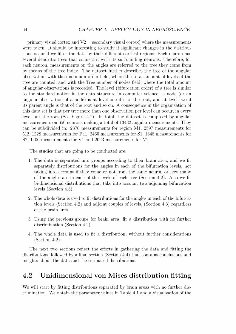
64 CHAPTER 4. APPLICATION IN NEUROSCIENCE

= primary visual cortex and V2 = secondary visual cortex) where the measurementswere taken. It should be interesting to study if significant changes in the distribu-tions occur if we filter the data by their different cortical regions. Each neuron hasseveral dendritic trees that connect it with its surrounding neurons. Therefore, foreach neuron, measurements on the angles are referred to the tree they come fromby means of the tree index. The dataset further describes the tree of the angularobservation with the maximum order field, where the total amount of levels of thetree are counted, and with the Tree number of nodes field, where the total amountof angular observations is recorded. The level (bifurcation order) of a tree is similarto the standard notion in the data structure in computer science: a node (or anangular observation of a node) is at level one if it is the root, and at level two ifits parent angle is that of the root and so on. A consequence in the organization ofthis data set is that per tree more than one observation per level can occur, in everylevel but the root (See Figure 4.1). In total, the dataset is composed by angularmeasurements on 650 neurons making a total of 13432 angular measurements. Theycan be subdivided in: 2370 measurements for region M1, 2597 measurements forM2, 1228 measurements for PrL, 2460 measurements for S1, 1348 measurements forS2, 1406 measurements for V1 and 2023 measurements for V2.

The studies that are going to be conducted are:

1. The data is separated into groups according to their brain area, and we fitseparately distributions for the angles in each of the bifurcation levels, nottaking into account if they come or not from the same neuron or how manyof the angles are in each of the levels of each tree (Section 4.2). Also we fitbi-dimensional distributions that take into account two adjoining bifurcationlevels (Section 4.3).

2. The whole data is used to fit distributions for the angles in each of the bifurca-tion levels (Section 4.2) and adjoint couples of levels, (Section 4.3) regardlessof the brain area.

3. Using the previous groups for brain area, fit a distribution with no furtherdiscrimination (Section 4.2).

4. The whole data is used to fit a distribution, without further considerations(Section 4.2).

The next two sections reflect the efforts in gathering the data and fitting thedistributions, followed by a final section (Section 4.4) that contains conclusions andinsights about the data and the estimated distributions.

4.2 Unidimensional von Mises distribution fitting

We will start by fitting distributions separated by brain areas with no further dis-crimination. We obtain the parameter values in Table 4.1 and a visualization of the

4.2. UNIDIMENSIONAL VON MISES DISTRIBUTION FITTING 65

Figure 4.1: Graphical visualization of the organization of the dataset.


global distribution in Figure 4.2.

µ κ a b NumSamplesM1 0.9586 6.7874 0.0435 2.7829 2370M2 0.8716 6.7658 0.0241 2.7387 2597PrL 1.0397 5.0904 0.0532 2.7622 1228S1 0.8977 5.8081 0.0372 2.7947 2460S2 1.0405 6.3850 0.0682 2.5094 1348V1 1.0630 5.7608 0.0413 2.7281 1406V2 0.9402 5.4111 0.0413 2.4604 2023All 0.9553 5.9437 0.0241 2.7947 13432

Table 4.1: Parameter values of truncated von Mises distributions of each groupaccording to the brain area, and the whole dataset.

Figure 4.2: Estimated truncated von Mises distribution for the entire dataset. Thisdistribution corresponds to the parameter values of the 9th row (named “All”) inTable 4.1.

Subsequently we will consider the bifurcations independently of the brain area.The distribution parameters are estimated to be those shown at the Table 4.2.

4.2. UNIDIMENSIONAL VON MISES DISTRIBUTION FITTING 67

µ κ a b NumSamplesBifurcation level 1 1.1152 6.1557 0.0849 2.7947 3160Bifurcation level 2 0.9881 6.1180 0.0214 2.7387 4382Bifurcation level 3 0.8722 6.4098 0.0331 2.6796 3656Bifurcation level 4 0.8176 6.7795 0.0284 2.7829 1704Bifurcation level 5 0.7749 6.7829 0.0968 1.8229 439Bifurcation level 6 0.7494 8.3659 0.1297 1.8358 78

Table 4.2: Estimated truncated von Mises distributions for the entire dataset sep-arated in 6 bifurcation levels. We can notice the emergence of a pattern whenexamining the values of the µ parameter, that seem to decrease when increasing thelevel we look at.

In the data set, bifurcations of level 7 and 8 were also present but their numberis too low (12 and 1 respectively) to obtain valuable information of the underlyingdistribution.

Now we proceed with the most restrictive univariate case, where bifurcations areobtained on brain areas separated groups. The resulting parameters are shown inTable 4.3.


M1 µ κ a b NumSamplesBifurcation level 1 1.0950 6.4282 0.0849 2.3636 503Bifurcation level 2 1.0025 6.7029 0.08460 2.7302 766Bifurcation level 3 0.8962 7.8967 0.0435 2.1037 696Bifurcation level 4 0.8274 7.3457 0.0607 2.7829 306Bifurcation level 5 0.832 8.8018 0.0968 1.8229 85

M2 µ κ a b NumSamplesBifurcation level 1 1.0591 6.4921 0.01245 2.4070 539Bifurcation level 2 0.9120 7.2924 0.0214 2.7387 810Bifurcation level 3 0.8 7.32 0.0331 1.9482 749Bifurcation level 4 0.73 8.4814 0.0284 1.9996 385Bifurcation level 5 0.6833 7.0187 0.1276 1.7037 92

PrL µ κ a b NumSamplesBifurcation level 1 1.1205 5.1347 0.1015 2.7622 434Bifurcation level 2 1.03 5.7942 0.0532 2.3905 424Bifurcation level 3 0.9379 4.0840 0.0901 2.4392 243Bifurcation level 4 0.9677 3.5071 0.0751 2.3062 95

S1 µ κ a b NumSamplesBifurcation level 1 1.0814 6.6099 0.972 2.7947 540Bifurcation level 2 0.9401 6.0594 0.0602 2.5562 772Bifurcation level 3 0.8109 5.7411 0.0372 2.6796 683Bifurcation level 4 0.7425 6.6456 0.0665 2.1260 340Bifurcation level 5 0.7018 4.6349 0.01402 1.6897 102

S2 µ κ a b NumSamplesBifurcation level 1 1.1944 7.3074 0.2317 2.5094 304Bifurcation level 2 1.0689 5.7819 0.18 2.4550 437Bifurcation level 3 0.9305 6.5320 0.0682 2.0386 379Bifurcation level 4 0.9219 6.7647 0.01734 2.2480 173

V1 µ κ a b NumSamplesBifurcation level 1 1.1579 5.423 0.1008 2.7281 379Bifurcation level 2 1.0764 5.6469 0.0594 2.7017 506Bifurcation level 3 0.9896 6.1741 0.0413 2.0317 350Bifurcation level 4 0.9564 5.4722 0.02502 2.0169 146

V2 µ κ a b NumSamplesBifurcation level 1 1.1469 5.6495 0.01145 2.2754 461Bifurcation level 2 0.9438 5.0379 0.0857 2.4604 667Bifurcation level 3 0.8681 5.9403 0.0413 2.2450 556Bifurcation level 4 0.8036 6.6848 0.0658 1.7391 259

Table 4.3: Estimated truncated von Mises distributions for the different brain areasand for the different bifurcation levels. We can notice how the decreasing µ patternis highly consistent appearing in every subgroup except for PrL and M1 in the fewersamples estimator (levels 4 and 5, respectively).

4.3. BIDIMENSIONAL VON MISES DISTRIBUTION FITTING 69

In all cases only the levels with enough information to conduct studies under reason-able reliability are shown. Not enough information was found about the remainingunanalyzed levels to create a descriptive distribution with meaningful parameters.Similarly, some of the 4 and 5 bifurcation levels contain few observations and there-fore the estimated distributions shall be used with care. These observed distributionspresent the apparent under observation property of containing the mean under thetruncation parameters a, b.

4.3 Bidimensional von Mises distribution fitting

We proceed now with the study of the data separated by bifurcation levels, wheretwo adjoining levels are used to fit a bivariate von Mises distribution, and marginaldistributions are subsequently obtained. See Table 4.4 for the parameter valuesand Figure 4.3 for the visualization of the bivariate distribution estimated frombifurcations 1 and 2.

Bif1-2 Bif2-3 Bif3-4 Bif4-5λ 0.1321 0.0069 0.0016 0µ1 1.1150 0.9924 0.8579 0.8192µ2 0.9793 0.8722 0.8175 0.7749κ1 6.1575 6.3501 6.8053 7.4951κ2 6.4512 6.4098 6.7795 6.7828a1 0.0849 0.0214 0.0331 0.0607b1 2.7947 2.7387 2.4392 2.7829a2 0.0214 0.0331 0.0284 0.0968b2 2.7387 2.6796 2.7829 1.8229

NumSamples 3160 3656 1704 439

Table 4.4: Estimated truncated bivariate von Mises distributions for pairs of bifur-cation levels from one to five in the whole dataset. We can notice that the estimationseems to show tendency to independence by a decreasing tendency in the λ param-eter. Also, there exists a decreasing tendency shown by both means µ1, µ2


Figure 4.3: Estimated bivariate truncated von Mises distribution for the joint dataof the bifurcation levels 1 and 2. The parameter values of this distribution are thosein the second column of Table 4.4 (named “Bif1-2”).

The marginal distributions of the variables are shown in Figure 4.4 and Figure 4.5.


Figure 4.4: Marginal distribution of the first component (Bifurcation 1) in the bi-variate case for Bifurcation levels 1 and 2 shown in Figure 4.3.

Figure 4.5: Marginal distribution of the second component (Bifurcation 2) in thebivariate case for Bifurcation levels 1 and 2 shown in Figure 4.3.

Now we begin with the study for the angles grouped by brain areas, see Tables4.5− 4.11.


M1 Bif1-2 Bif2-3 Bif3-4 Bif4-5λ 1.182×10−4 0.2258 4.257×10−6 1.639×10−6

µ1 1.0950 1.0044 0.8753 0.7845µ2 0.9851 0.8959 0.8274 0.8032κ1 6.4282 6.6223 7.4440 8.9957κ2 6.6112 7.9025 7.3457 8.8018a1 0.0849 0.0846 0.1366 0.1037b1 2.3636 2.7302 1.9245 1.5883a2 0.0846 0.0435 0.0607 0.0968b2 2.7302 2.1037 2.7829 1.8229

NumSamples 503 696 306 85

Table 4.5: Estimated truncated bivariate von Mises distributions for pairs of bifur-cation levels from one to five in the M1 region. Here the decreasing tendency in theλ parameter is not followed by either Bif1-2 or by Bif2-3.

M2 Bif1-2 Bif2-3 Bif3-4λ 5.626×10−5 0.0332 0.1304µ1 1.0591 0.9050 0.7810µ2 0.8990 0.7999 0.7297κ1 6.4921 7.3429 7.2363κ2 7.6665 7.3200 8.4832a1 0.1245 0.0214 0.0484b1 2.4070 2.1460 1.9482a2 0.0494 0.0331 0.0284b2 2.1460 1.9482 1.9996

NumSamples 539 749 385

Table 4.6: Estimated truncated bivariate von Mises distributions for pairs of bifur-cation levels from one to four in the M2 region.


PrL Bif1-2 Bif2-3 Bif3-4λ 3.031×10−5 0.4010 1.5938×10−4

µ1 1.1181 1.0418 0.9795µ2 1.0300 0.9369 0.9676κ1 5.0894 5.0658 3.2597κ2 5.7942 4.1053 3.5052a1 0.1015 0.0532 0.0901b1 2.7622 2.3905 2.1333a2 0.0532 0.0901 0.0751b2 2.3905 2.4392 2.3067


Table 4.7: Estimated truncated bivariate von Mises distributions for pairs of bifur-cation levels from one to four in the PrL region.

S1 Bif1-2 Bif2-3 Bif3-4 Bif4-5λ 0.0388 2.6816×10−6 1.4244×10−5 0.7758µ1 1.0813 0.9418 0.7927 0.7224µ2 0.9462 0.8109 0.7425 0.6954κ1 6.6073 6.0741 5.6382 6.4157κ2 6.2157 5.7432 6.6491 4.7152a1 0.0972 0.0602 0.0414 0.1093b1 2.7947 2.5562 2.6796 2.1260a2 0.0602 0.0372 0.0665 0.1402b2 2.5562 2.6796 2.1260 1.6897

NumSamples 540 683 340 102

Table 4.8: Estimated truncated bivariate von Mises distributions for pairs of bifur-cation levels from one to five in the S1 region.


S2 Bif1-2 Bif2-3 Bif3-4λ 3.3963×10−4 0.3654 0.8097µ1 1.1944 1.0740 0.9155µ2 1.0492 0.9294 0.9210κ1 7.3069 5.9562 7.5549κ2 5.9968 6.5507 6.8241a1 0.2317 0.1800 0.0682b1 2.5094 2.4550 1.9599a2 0.2185 0.0682 0.1734b2 2.4450 2.0386 2.2480


Table 4.9: Estimated truncated bivariate von Mises distributions for pairs of bifur-cation levels from one to four in the S2 region.

V1 Bif1-2 Bif2-3 Bif3-4λ 2.2086×10−5 0.5036 3.6420×10−5

µ1 1.1579 1.0779 0.9821µ2 1.0840 0.9885 0.9565κ1 5.4260 6.0449 5.6997κ2 5.8202 6.2072 5.4751a1 0.1008 0.1283 0.0428b1 2.7281 2.5066 1.9700a2 0.1283 0.0413 0.2502b2 2.5066 2.0317 2.0169


Table 4.10: Estimated truncated bivariate von Mises distributions for pairs of bifur-cation levels from one to four in the V1 region.

4.4. CONCLUSIONS AND FURTHER STUDIES 75

V2 Bif1-2 Bif2-3 Bif3-4λ 0.5981 1.5503×10−6 3.5550×10−5

µ1 1.1430 0.9412 0.8655µ2 0.9530 0.8681 0.8036κ1 5.6930 4.9758 5.5421κ2 4.8082 5.9418 6.6849a1 0.1145 0.0881 0.0413b1 2.2754 2.4604 2.2450a2 0.1262 0.0413 0.0658b2 2.3372 2.2450 1.7391


Table 4.11: Estimated truncated bivariate von Mises distributions for pairs of bifur-cation levels from one to four in the V2 region.

Similarly as before, distributions obtained with a sample size < 200 shall be inter-preted with care.

4.4 Conclusions and further studies

1. All considered univariate distributions satisfy that µ1 ∈ [a, b] and all bivariatedistributions satisfy that (µ1, µ2) ∈ [a1, b1] × [a2, b2] (or at least, µ1 ∈ [a1, b1]and µ2 ∈ [a2, b2]) which together with the particular values of the truncationparameters can yield information about characteristic behavior of dendriticarborizations or dendritic trees. Also, as briefly introduced before, there is aremarkable tendency on the mean parameter that seems to decrease accord-ingly to the increase of the bifurcation level. This could be initially consideredan indicator of an angles overall decrease of value when bifurcation level incre-ments, however truncation and concentration parameters do not show directsupport of this hypothesis as concentration does not seem to steadily increaseor decrease and truncation parameters do not show to be significantly differentin any of the levels for which we have enough data.

2. Truncation parameters varied from the minimum a parameter, a = 0.0241 tothe maximum b, b = 2.7947 which correspond to 1◦ 3′ and 160◦ 12′ respectively.It can be noted that dendritic angles do not surpass 180◦ which could be con-sidered an angle where the new level “does not gain distance from the origin”.This functional appreciation could suggest that in the design and developmentof dendritic trees, there is an interest to grow distant from the neuron’s somawith new bifurcations, which could be directly related to the need of establish-ing new connections with other neurons. Angles superior to that amount canbe considered “to go backwards” respect to the origin point and seem not very


beneficial when trying to establish new connections with distant neurons. Theminimal angle could be also viewed as the angle that transports subsequentbifurcations more in space. It can be hypothesized solely from these appreci-ations that a tendency of higher angles in the primary bifurcation levels thatcould be reflected in the mean and concentration of the data would be present,and when growing the bifurcation levels,the angle separation would decrease.However, this is not confirmed at an experimental level, and it can also be be-cause the additional interest to grow in length coupled with the hypothesizedinterest to grow in width. These notions can further induce to consider thatin a 3-dimensional space, dendritic trees construction shows interest in width,length and depth expansion as is trying to maximize their communication ca-pabilities with other neurons, with no preference for any of them identified inthe data.

3. The comparisons between the univariate distributions in the separations withbrain area criteria or bifurcation criteria revealed few overall differences for allof them, behaving remarkably similar despite the differentiation criteria ap-plied to the dataset. However, when dividing the data with bifurcation criteriacoupled with the brain area criteria, the resulting sub-datasets could have pre-sented not enough samples to conduct reliable analysis, specially when dealingwith bifurcation levels beyond three. All distributions showed proximity tosymmetry and relatively high concentration around their mean.

4. Bivariate distributions of bifurcation levels showed an overall remarkable prox-imity to independence, with many of them showing values below λ = 10−4 withthe optimization techniques that were applied for parameter estimation. In theglobal bifurcations study, a consistent decreasing tendency on λ was observed,which itself could suggest that the influence of bifurcations on a level on theimmediately higher may decrease as the level increases. However, it is alsosuggested that in any of the cases such influence would not represent a non-small contributing factor, as the highest lambda value in this study was foundto be λ = 0.1321. When the study was conducted region-wise, higher valuesof the λ parameter were found, but still were considered small and insufficientfor explanations with clearly identified elements. The consistent higher valueof the λ parameter in Bif2-3 w.r.t. the other bifurcation pairs in 3 of the 8tables may suggest a localized phenomena worth of study.

It is still not clear that dendritic ramifications do not respond at a biologicallevel to their context immediate connection needs or also that the bifurcationlevels are not locally related to their previous bifurcation parent angles.

5. Some estimations that produced more distinct results are considered and con-cluded to be highly contaminated by the lack of a proper number of samples.Distributions of similar configurations to the obtained in this study may sufferfrom parameter poor quality estimations specially regarding truncation pa-

4.4. CONCLUSIONS AND FURTHER STUDIES 77

rameters, where the less likely individuals (in this case, by the expected shapeof the distribution) are the truncation limits of the distribution.

Further studies could include observing the behavior of n−dimensional truncatedvon Mises distributions when analyzing the dendritic trees and all their possible sub-divisions and to obtain new discrimination criteria that allows to select appropriatesubgroups of the dataset showing unknown relationships currently unobserved bythe conducted subgroup selection criteria. For example, it could be useful to ex-amine the bifurcation levels locally w.r.t. their parent bifurcations to see it furtherpatterns arise, or if the obtained decreasing mean pattern is additionally supportedby findings that allow for better explanations of the observed angular behaviors.


Chapter 5

Conclusions and future work

In this work we have developed the theoretical framework of the truncated von Misesdistribution. This objective was achieved by:

1. The successful determination of the expressions of maximum likelihood estima-tors. For both univariate and bivariate cases, maximum likelihood estimatorsof the truncation parameters were found in isolated and solely sample depen-dent form, while the other parameters showed interdependency also in bothcases. A system of Karush-Kuhn-Tucker equations was used to model andsolve the remaining parameters in a numerical estimation approach.

2. Obtaining the moments of the univariate case and existing relationships be-tween them.

3. The properties of both bivariate and univariate case, specially the results con-cerning the additional manipulability and shapes that the distribution canpresent when modifying the truncation parameters. They allow us to see themost characteristic particularities of the truncated case, where a similar distri-bution in the remaining parameters can show remarkable distinct behaviors,such as being a strictly increasing or strictly decreasing function, presentingsymmetry or not, or concentrating its positive support in a sub-interval asshort as we let it be. In this work, parameter conditions for those cases havebeen gathered for both univariate and bivariate cases.

4. The bivariate case and studies of the shape and behavior of marginal andconditional resulting probability distributions. We determined that every con-ditional distribution on a truncated bivariate von Mises distribution is a trun-cated univariate von Mises distribution independently of the value of the λparameter. For the case of the marginal distribution, we concluded that onlyfor parameter λ = 0, that is, independence between the variables of the bivari-ate, the distribution behaves like a truncated univariate von Mises distribution.When variables show some degree of dependency, the resultant marginal dis-tribution is not von Mises, but a potentially bimaximal distribution (otherwiseunimodal). We concluded 4 different cases based on the configuration of the

79

80 CHAPTER 5. CONCLUSIONS AND FUTURE WORK

truncation parameters that allowed us to isolate the parameter ranges andconfigurations where the truncated marginal von Mises shows all its differentbehaviors. More concretely, we were able to identify the parametric circum-stances for a bimaximal distribution to be bimaximal, to present either one oftwo or two global maxima and how the minimum value is not at the mean valueµ1 in the first case but necessarily at the second. Also, the parametric circum-stances for a unimodal distribution to be unimodal and for it to present itsmaximum at µ1 (or not and how) were identified, leaving no behavior or shapeof the marginal distribution unclassified and undocumented by our analysis.

The theoretical extent of this work also covers appropriate introductions and ease-ments regarding the use of Bessel functions and the indefinite integral of (2.3), thatare of necessary consideration if further work is to be conducted on the subjectmatter.

Future lines of research can be orientated to further simplify the expressions thatdescribe the different calculations conducted in this work, finding expression equiv-alences that show clearly unknown but present properties or are more efficientlyanalyzable to more accurately derive the existent results. This could benefit theexpressions involving the indefinite integrals of moments, maximum likelihood esti-mators and expectancies showed in this masters thesis.

Relatedly, research on integral calculus to further push away the limits of math-ematical tractability and work with infinite series may be of direct effect on the finalexpressions that were reported here. Works and results regarding Bessel functions,specially concerning generalizations that cover the case where the integral coeffi-cients are not restricted to a 2π−length (or any multiple of π) can be of immediateapplication.

Another line of research regarding estimators could be developments that moreefficiently take into account the truncation limitations of the data and could bythe mathematical properties of the distribution create better approximations, thusaddressing the interdependence of the parameters that the current and applied esti-mation techniques (maximum likelihood estimation) show in a more elaborated way.

This work is also susceptible to continuation in calculations that further describethe truncated von Mises distribution. Some examples of this may include samplemean and sample mean resultant length distributions, among others.

Bibliography

Abramowitz, M. and Stegun, I. (1964). Handbook of Mathematical Functions: WithFormulas, Graphs, and Mathematical Tables. Applied Mathematics Series. DoverPublications.

Ballesteros-Yanez, I., Benavides-Piccione, R., Bourgeois, J.-P., Changeux, J.-P.,and DeFelipe, J. (2010). Alterations of cortical pyramidal neurons in mice lackinghigh-affinity nicotinic receptors. Proceedings of the National Academy of Sciences,107(25):11567–11572.

Bistrian, D. A. and Iakob, M. (2008). One-dimensional truncated von mises distri-bution in data modeling. Annals of Faculty of Engineering Hunedoara.

Gradshteyn, I. S. and Ryzhik, I. M. (2007). Table of Integrals, Series, and Products.

Jupp, P. E. and Mardia, K. V. (1989). A unified view of the theory of directionalstatistics, 1975-1988. International Statistical Review, 57(3):261–294.

Mardia, K. and Jupp, P. (2000). Directional Statistics. Wiley Series in Probabilityand Statistics.

Mardia, K. V., Hughes, G., Taylor, C. C., and Singh, H. (2008). A multivariatevon mises distribution with applications to bioinformatics. Canadian Journal ofStatistics, 36(1):99–109.

Mardia, K. V. and Voss, J. (2011). Some fundamental properties of a multivariatevon Mises distribution. ArXiv e-prints.

Rosenheinrich, W. (2013). Tables of some idefinite integrals of bessel functions.University of Applied Sciences Jena.

Singh, H. (2002). Probabilistic model for two dependent circular variables.Biometrika, 89(3):719–723.

81

Documents

CONTRIBUTIONS TO THE TRUNCATED VON MISES …cig.fi.upm.es/thesis/master/Contributions to the truncated von... · CONTRIBUTIONS TO THE TRUNCATED VON MISES ... dos de este trabajo para