R. J. Moffat Thermosciences Division,

Department of Mechanical Engineering, Stanford University,

Stanford, Calif. 94305

Contributions to the Theory of Single-Sample Uncertainty Analysis

Introduction

Uncertainty Analysis is the prediction of the uncertainty interval which should be associated with an experimental result, based on observations of the scatter in the raw data used in calculating the result. In this paper, the process is discussed as it applies to single-sample experiments of the sort frequently conducted in research and development work. Single-sample uncertainty analysis has been in the engineering literature since Kline and McClintock's paper in 1953 [1] and has been widely, if sparsely, practiced since then. A few texts and references on engineering experimentation present the basic equations and discuss its importance in planning and evaluating experiments (see Schenck, for example [2]). Un­certainty analysis is frequently linked to the statistical treatment of the data, as in Holman [3], where it may be lost in the fog for many student engineers. More frequently, only the statistical aspects of data interpretation are taught, and uncertainty analysis is ignored.

For whatever reasons, uncertainty analysis is not used as much as it should be in the planning, development, in­terpretation, and reporting of scientific experiments in heat transfer and fluid mechanics. There is a growing awareness of this deficiency among standards groups and funding agencies, and a growing determination to insist on a thorough description of experimental uncertainty in all technical work. Both the International Standards Organization [4] and the American Society of Mechanical Engineers [5] are developing standards for the description of uncertainties in fluid-flow measurements. The U. S. Air Force [6] and JANNAF [7] each have handbooks describing the appropriate procedures for their classes of problems. The International Committee on Weights and Measures (CIPM) is currently evaluating this issue [8].

The prior references, with the exception of Schenck and, to a lesser extent, Holman, treat uncertainty analysis mainly as a process for describing the uncertainty in an experiment, and end their discussion once that evaluation has been made. The present paper has a somewhat different goal: to show how uncertainty analysis can be used as an active tool in developing a good experiment, as well as reporting it.

The concepts presented here were developed in connection with heat transfer and fluid mechanics research experiments of moderately large size (i.e., larger than a breadbox and smaller than a barn) and which may frequently require three

Contributed by the Fluids Engineering Division and presented at the 1980-1981 AFOSR-HTTM Conference on Complex, Turbulent Flows; Comparison of Computation and Experiment, September, 1981, Manuscript received by the Fluids Engineering Division, May 11, 1981.

to six months to "debug." The "debugging" process involves modifying the rig or the data-reduction program to remove, or account for, errors introduced by the apparatus and procedure. This phase ends when the experiment has ac­ceptably small fixed errors over its entire operating range. In the early stages, when attention is focused on improving uniformity and stability, what is needed is a technique for evaluating each irregularity in the data, to see whether it is significant or just the result of random variations in the data. In the later stages of development, it is important to evaluate the significance of any differences between the results from the new apparatus and the accepted results for the same nominal case. Once the apparatus is commissioned for data-taking, the test runs typically involve hundreds of data points, taken over a period of months, which are to be compared with each other and with data from other sources. Each data point will probably be taken only once, so these are single-sample experiments - there will be no averaging of the results. What is needed in this phase is a method of evaluating the day-to­day scatter about the mean trends, and the significance (if any) of both the trends and the scatter. The final stage, reporting the results and comparing them with the existing literature, requires a method of analyzing the uncertainty which permits a strict comparison with the works of others, at different laboratories and at different times.

As the above paragraph points out, uncertainty analysis results can provide decision criteria in five different stages of an experiment. There are three different types of information which can be obtained from an uncertainty analysis for use in these five situations, as will be discussed later in this paper. It is important, however, that any predicted uncertainty be really believable to the experimenter; serious day-to-day decisions will be based upon it - for example, whether to tear down the rig for repair or to press on. The researcher must have confidence both in the method used and the selection criteria by which elements are included in the tally of un­certainties.

The present paper concerns uncertainty analysis applied to single-sample experiments which have negligible fixed error. Not all experiments have these two important properties. Many industrial experiments use data averaging (i.e., multiple samples), and many have significant fixed errors compared to the residual random error after averaging. There is an im­portant work by Abernethy et al. [6] which describes procedures for dealing with multi-sample experiments in which the bias error is significant and may even dominate the final uncertainty. Abernethy's procedure covers cases in

250/Vol. 104, JUNE 1982 Transactions of the ASME Copyright © 1982 by ASME Downloaded 30 Aug 2010 to 139.82.149.123. Redistribution subject to ASME license or copyright; see http://www.asme.org/terms/Terms_Use.cfm

which several results are averaged (not covered by the present method) and where the different subordinate results combined in calculating the principal result may have different degrees of freedom (not covered by the present method). It is a powerful and general method, but complex. The uncertainty defined by Abernethy's method is the sum of the "bias" (the estimated fixed error) and " t 9 5 x S " (accounting for the random errors). The term S is the standard deviation of the sample, and t95 is the 95 percent confidence level factor from the two-tailed Student's t-distribution. When the sample has 30 or more degrees of freedom, t95 can be used as 2.00 for most purposes. The most important conceptual difference between Abernethy's method and the present one is in the definition of uncertainty. The present paper defines un­certainty in terms of only the random components of ex­perimental error, while Abernethy et al. include the fixed error in the final presentation of uncertainty. For experiments with negligible fixed error, this difference in definition has no effect.

The Zero-Centered Experiment

The objective of experimental work is to learn the true value of some result. Real experiments, however, are subject to both fixed errors (biases) and random errors (precision errors). An experiment which has no fixed error will produce the true value as the average of many trials and, in this paper, will be called a zero-centered experiment. The name was chosen because this ideal experiment has zero fixed error, and its measured results are centered about the true value.

The zero-centered experiment is a goal, not often a reality. Experiments whose outcome is highly variable compared with the precision with which it can be measured might be con­sidered zero-centered, such as scorekeeping in bowling, or golf, or studying turbulence. In those cases the process itself generates large random excursions, yet the measurement of the result may be quite precise. From a practical standpoint, some other experiments can be made zero-centered by refining them to the point where their fixed error is negligibly small compared to their precision index. This can frequently be done for single-sample experiments, but only rarely for ex­periments where the results will be averaged. Averaging reduces the effect of random errors but does not affect the fixed error; hence an experiment which might qualify as zero-centered if run as a single-sample experiment might not qualify if sixteen runs were averaged. In the latter case, the fixed error would be unchanged while the precision index of the average would be reduced by a factor of four.

The whole process of "debugging" an experiment, so familiar to all experimentalists, is aimed at removing the causes of recognized fixed errors.

It is important to this "debugging" process that the un­certainties in the experiment be assessed conservatively. Conservatively, in this case, means "as tightly as can be justified," since inflating the uncertainties expands the ambiguity band within which false results may be accepted as true. Inflating the uncertainty estimates through false modesty is not "conservative" but, in fact, helps conceal faults in the experiment.

Because of the importance of working with the minimum uncertainty which must be expected in a given experiment, one must have clearly defined criteria for deciding which terms are to be retained in the analysis and which are to be left out. It is helpful, first, to review the sources of scatter in data, to classify the various sources, and to decide how and when to include their effects in an uncertainty analysis.

The Sources of Scatter in Data

The term "scatter" is a qualitative descriptor of the variance in data, the extent to which the individual values differ from the mean. Where does this scatter come from?

Real processes are affected by more variables than the experimenters wish to acknowledge. A general representation is given in equation (1), which shows a result, R, as a function of a long iist of real variables. Some of these are under the direct control of the experimenter, some are under indirect control, some are observed but not controlled, and some are not even observed.

R=R(xl,X2,xi,x4,x5,X(>, . . . ,JC/v) (1)

An experiment aimed at studying the result, R, as a func­tion of one or more variables will probably be designed as a partial derivative experiment, varying one or more of the controlled variables, hoping that the rest will remain constant. The experimenters wish is illustrated in equation (2), which treats everything to the left of the semicolon as a controlled, or at least observed, variable, and all the other terms as parameters which are not expected to change or be important during the experiment. The fact that this is an artificial distinction is brought home when all the controlled variables are held constant and the results still display scatter.

R=R(Xl,X2,X},X4; x5,x6, . . . ,xN) (2)

Time is a monotonic variable in every experiment, and many factors outside an experiment change with time. The effect of time may be direct, as in the change of state of a system during a transient or indirect, as when a supposedly steady parameter displays timewise variations. There are short-term (microseconds, seconds, minutes) and long-term (hours, days, months, and years) effects. Many processes are unsteady, to some extent, and then the time constant of the system and the instruments becomes important. When an unsteady system is examined through instruments whose time constants are different from that of the system and also different from each other, the different phase lags of the different instruments will result in data which show random, uncorrelated variations-jitter in the instruments yields scatter in the data, which, in turn, produces scatter in the result.

Human judgment is also a variable. Different observers examining an instrument face may read it differently on each successive trial, even though the display might remain ab­solutely fixed.

Instrument calibrations are not the same from instrument to instrument, even of the same nominal type and made by the same manufacturer.

The present method of analysis is aimed at helping the experimenter properly account for the effects of judgment, jitter, and calibration so the real behavior of the process can be seen. Then, if there are undesired factors affecting the process, their effects can be recognized and dealt with.

There remains the problem of deciding which effects should be included in the uncertainty analysis and how they should be treated. This is discussed in the next section.

Bias, Precision, and Uncertainty

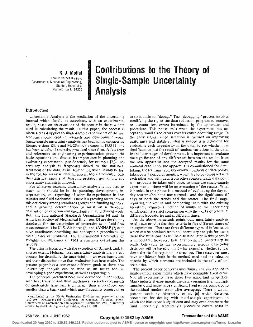
There are two different concepts to deal with: statistical operations and uncertainty. Statistics can be applied only to data which exist; uncertainty is a prediction. The terms "bias" and "precision" are illustrated in Fig. 1(a). The points on the abscissa represent a set of data - 30 measurements of the variable x. The curve shown is a normal distribution curve representing the frequency of occurrence of different values of x in an infinitely large sample (i.e., the parent population). The difference between the mean value of the data, x, and the true value is the "bias error" or "fixed error" of the data set. The dispersion of the curve, measured by the standard deviation, ax, is a property of the distribution function, not of the set of 30 data points. The standard deviation can only be estimated, from any finite set of data. The estimator of the standard deviation is Sx, a value calculated from the data.

Journal of Fluids Engineering JUNE 1982, Vol. 104/251

Downloaded 30 Aug 2010 to 139.82.149.123. Redistribution subject to ASME license or copyright; see http://www.asme.org/terms/Terms_Use.cfm

Either ax or Sx can be called a "precision index." Witness lines in Fig. 1(a) show the area enclosed by lines spaced 2ax

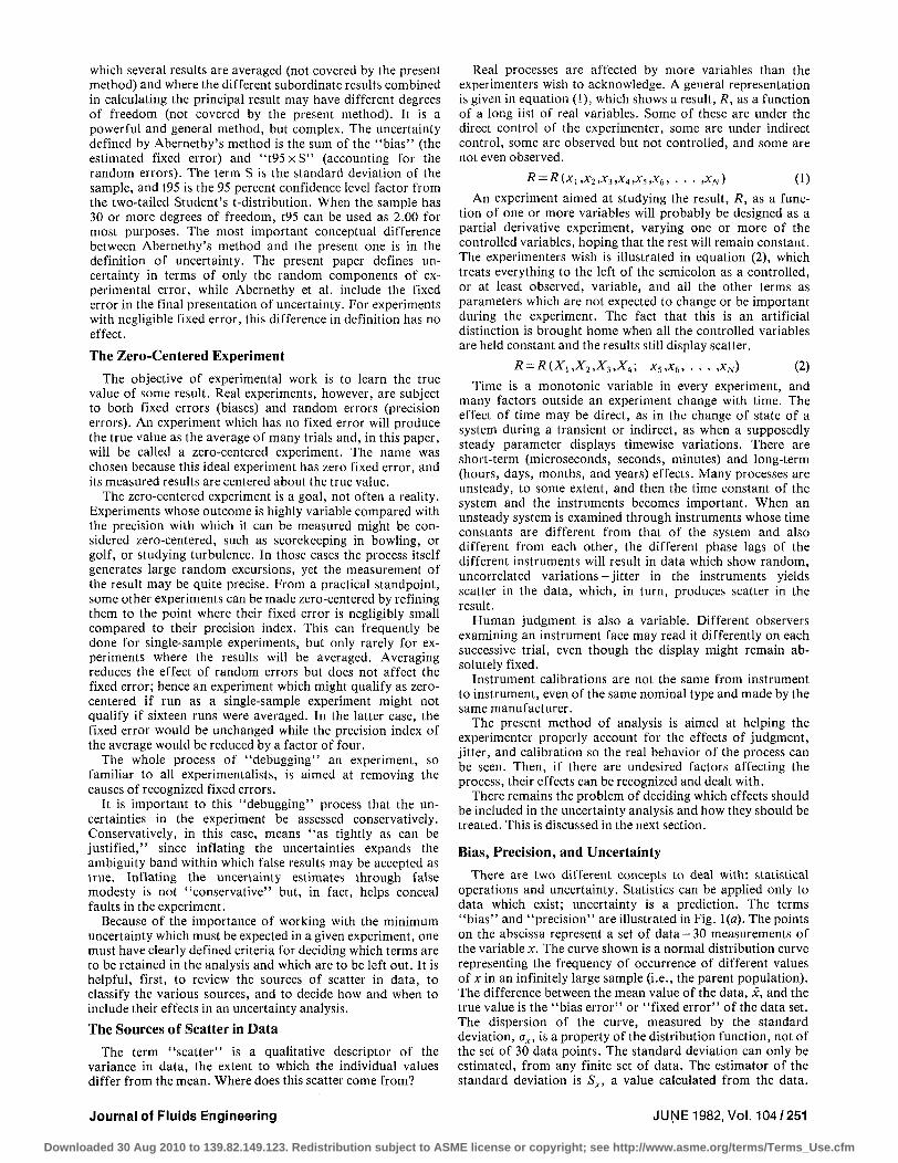
apart, representing approximately 95 percent of the total area. Uncertainty is illustrated in Fig. 1(b), which shows a single

data point, x, and a dashed curve, again a normal distribution curve. Each point on the curve in Fig. \(b) represents the probability that the mean would lie at that location if a large set of data were taken.

The curve in Fig. \(b) can be constructed about the 'measured value x only if ax is known, and that is the main objective of the present paper: developing a method for estimating the value of ax for the population of data from which the one sample, x, was taken.

The witness lines in Fig. 1(b) are drawn at the ±2<JV points, to include approximately 95 percent of the area under the curve. For this case, the uncertainty prediction is expected to be reliable with 95 percent confidence. Another way of describing this is to say that the mean value is expected to fall within those bounds 19 times out of 20. Yet another is to say that the odds are 20/1 that the mean lies within those bounds.

The dashed curve in Fig. 1(b) is drawn exactly centered about the measured data point; no offset is shown which would account for any fixed error. This is because there is no way to estimate the fixed error in a set of measurements based on those data alone. The dispersion is all that can be estimated. The standard deviation estimator, Sx, will be within a few percent of ax if 30 observations are made.

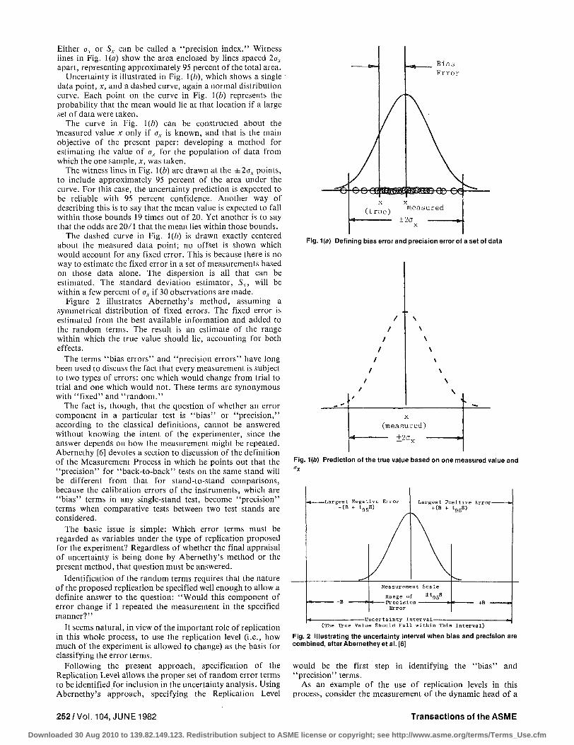
Figure 2 illustrates Abernethy's method, assuming a symmetrical distribution of fixed errors. The fixed error is estimated from the best available information and added to the random terms. The result is an estimate of the range within which the true value should lie, accounting for both effects.

The terms "bias errors" and "precision errors" have long been used to discuss the fact that every measurement is subject to two types of errors: one which would change from trial to trial and one which would not. These terms are synonymous with "fixed" and "random."

The fact is, though, that the question of whether an error component in a particular test is "bias" or "precision," according to the classical definitions, cannot be answered without knowing the intent of the experimenter, since the answer depends on how the measurement might be repeated. Abernethy [6] devotes a section to discussion of the definition of the Measurement Process in which he points out that the "precision" for "back-to-back" tests on the same stand will be different from that for stand-to-stand comparisons, because the calibration errors of the instruments, which are "bias" terms in any single-stand test, become "precision" terms when comparative tests between two test stands are considered.

The basic issue is simple: Which error terms must be regarded as variables under the type of replication proposed for the experiment? Regardless of whether the final appraisal of uncertainty is being done by Abernethy's method or the present method, that question must be answered.

Identification of the random terms requires that the nature of the proposed replication be specified well enough to allow a definite answer to the question: "Would this component of error change if I repeated the measurement in the specified manner?"

It seems natural, in view of the important role of replication in this whole process, to use the replication level (i.e., how much of the experiment is allowed to change) as the basis for classifying the error terms.

Following the present approach, specification of the Replication Level allows the proper set of random error terms to be identified for inclusion in the uncertainty analysis. Using. Abernethy's approach, specifying the Replication Level

l a s Error

Fig. 1 (a) Defining bias error and precision error of a set of data

(measured)

— ±2av -

Fig. 1(b) Prediction of the true value based on one measured value and

(The True Value Should Fal l within This Interval)

Fig. 2 Illustrating the uncertainty interval when bias and precision are combined, after Abernethey et al. [6]

would be the first step in identifying the "bias" and "precision" terms.

As an example of the use of replication levels in this process, consider the measurement of the dynamic head of a

252/Vol. 104, JUNE 1982 Transactions of the ASME

Downloaded 30 Aug 2010 to 139.82.149.123. Redistribution subject to ASME license or copyright; see http://www.asme.org/terms/Terms_Use.cfm

gas stream using a pitot-static probe. The observed pressure difference (total to static) for any single observation may differ from the actual pressure difference at that instant due to several errors:

P ind =P.ia + Et + E2+E3 +E4+ES + E6+E1

where

E\ = transducer calibration error, E2 = probe geometry error, E3 = probe misalignment error, E4 = shear displacement error, Es = turbulence-induced error, E6 = time-varying excursion, and E-i = scale-reading interpolation error.

For any one observation, each of these errors has a definite value, and only if we consider possible replications is it even appropriate to ask whether that error should be called "fixed" or "random."

To designate an error as "random," a type of replication must be identified which allows that error to take on different values on each repeated trial. Consider the simplest possible replication of the experiment described above. Nothing is allowed to change; we simply photograph the face of the indicator and read the pressure difference from the photograph, several times. If each is an independent ob­servation (for example, by using different observers for each reading), then the scale-reading interpolation error will be the only random variable and the only term which should be included in calculating the uncertainty in the measured pressure. There are only limited uses for that particular estimate of uncertainty, for example to answer the question, "Is there any chance of measuring the pressure within ±1 percent using this type of pressure indicator?"

As a second try, instead of making repeated observations on a single photograph, suppose that several independent observations were made of the face of the indicator, while the system was running. In addition to the scale-interpolating error, any time-varying excursions in the reading would also be sampled by this new replication, and both would be components of the uncertainty. This level of replication acknowledges the unsteadiness in the readings as well as the interpolation error, and is the lowest level ever really en­countered in the laboratory. Repeated trials with the same apparatus and no real change in the system behavior will display scatter about their mean value consistent with the uncertainty calculated at this level.

It would be possible to define a new level of replication each time one new constraint was relaxed - each time increasing the number of terms which should be included in the calculation of " the" uncertainty in the measured pressure. The most general replication would be if the probe was removed after each reading, exchanged for another probe which was similar but of different identity, and put back into a similar but different tunnel, and, for every measurement, every in­strument used was exchanged for another one, again similar but different. At this level, every factor is a variable, and every factor should appear in the uncertainty analysis. The resulting prediction of uncertainty would be appropriate for comparing the new data with data from other sources, in different laboratories, at different times, for nominally similar conditions.

It should be apparent by now that the uncertainty in a measurement has no single value which is appropriate for all uses. The uncertainty in a measured result can take on many different values, depending on what terms are included. Each different value corresponds to a different replication level, and each would be appropriate for describing the uncertainty associated with some particular measurement sequence. In Abernethy's parlance, each replication level divides the

I N I T I A L I Z A T I O N —

i

YES

( START ~)

/ READ 7

t GO TO

S U B R O U T I N E F - i ( X j x s )

•i i - i

SQ - 0

s ) GO TO S U B R O U T I N E

3 F / 3 x .

t - (H^ - . ) 2

1

5G = <5C + E

c

1 i - i + 1

- < ^ < N^>

NO

<SF - / I c "

, t , / P R I N T 7

/ F , 6 F /

t STOP )

— - > • -- ~f SUBROUTINE " \ ^ 3 F / 3 X i J

t GO TO A

S U B R O U T I N E F

+ £ i = f < X l X i + £ i -

E 1 i l l

— -4

i F - F

3F + E i ~ C i 3 x , 2 E

i L

" ( RETURN ")

. . , x N )

. , x s )

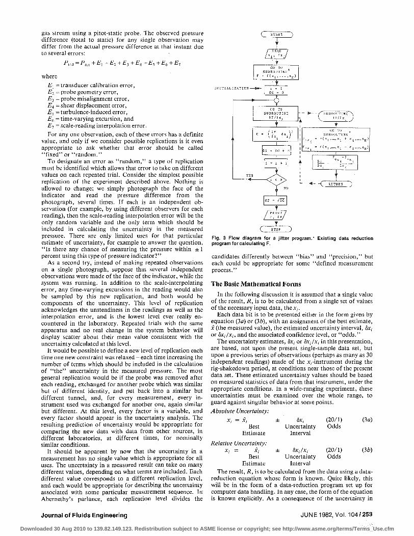
Fig. 3 Flow diagram for a jitter program.* Existing data reduction program for calculating F.

candidates differently between "bias" and "precision," but each could be appropriate for some "defined measurement process."

The Basic Mathematical Forms

In the following discussion it is assumed that a single value of the result, R, is to be calculated from a single set of values of the necessary input data, the xt.

Each data bit is to be presented either in the form given by equation (3a) or (3b), with an assignment of the best estimate, x (the measured value), the estimated uncertainty interval, 5A", or bXj/Xj, and the associated confidence level, or "odds."

The uncertainty estimates, &x, or bXj/x, in this presentation, are based, not upon the present single-sample data set, but upon a previous series of observations (perhaps as many as 30 independent readings) made of the x,-instrument during the rig-shakedown period, at conditions near those of the present data set. These estimated uncertainty values should be based on measured statistics of data from that instrument, under the appropriate conditions. In a wide-ranging experiment, these uncertainties must be examined over the whole range, to guard against singular behavior at some points.

Absolute Uncertainty:

Xi = Xj ± bx, (20/1) (3a) Best Uncertainty Odds

Estimate Interval

Relative Uncertainty: Xi = Xi ± bXj/Xj (20/1) (ib)

Best Uncertainty Odds Estimate Interval

The result, R, is to be calculated from the data using a data-reduction equation whose form is known. Quite likely, this will be in the form of a data-reduction program set up for computer data handling. In any case, the form of the equation is known explicitly. As a consequence of the uncertainty in

Journal of Fluids Engineering JUNE 1982, Vol. 104/253

Downloaded 30 Aug 2010 to 139.82.149.123. Redistribution subject to ASME license or copyright; see http://www.asme.org/terms/Terms_Use.cfm

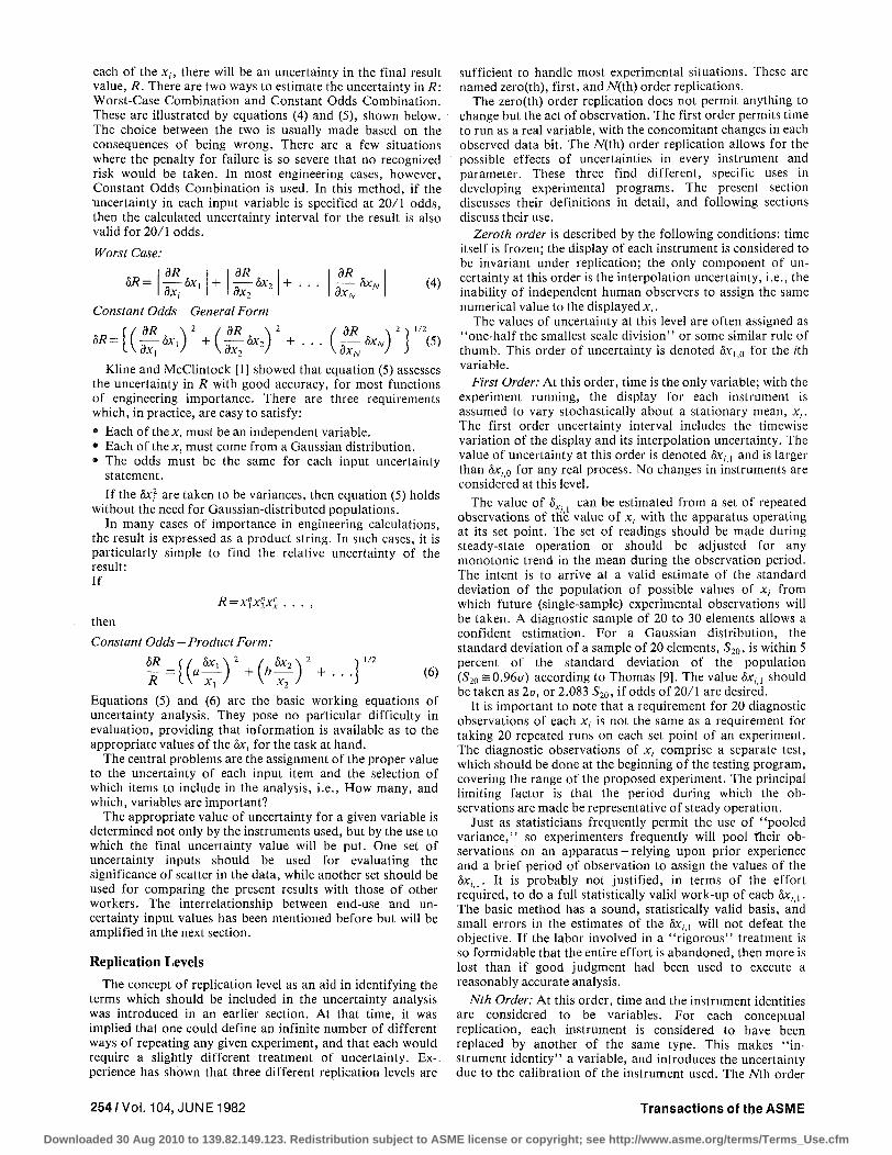
each of the x,, there will be an uncertainty in the final result value, R. There are two ways to estimate the uncertainty in R: Worst-Case Combination and Constant Odds Combination. These are illustrated by equations (4) and (5), shown below. The choice between the two is usually made based on the consequences of being wrong. There are a few situations where the penalty for failure is so severe that no recognized risk would be taken. In most engineering cases, however, Constant Odds Combination is used. In this method, if the •uncertainty in each input variable is specified at 20/1 odds, then the calculated uncertainty interval for the result is also valid for 20/1 odds.

Worst Case:

dR T—&*i dXj +

dR 7 &x2 dx2

+ . . . dR

bxN dxN

Constant Odds — General Form

Kline and McClintock [1] showed that equation (5) assesses the uncertainty in R with good accuracy, for most functions of engineering importance. There are three requirements which, in practice, are easy to satisfy:

• Each of the x, must be an independent variable. • Each of the xt must come from a Gaussian distribution. • The odds must be the same for each input uncertainty

statement.

If the bx} are taken to be variances, then equation (5) holds without the need for Gaussian-distributed populations.

In many cases of importance in engineering calculations, the result is expressed as a product string. In such cases, it is particularly simple to find the relative uncertainty of the result: If

R=x1xbiXLx

then

Constant Odds — Product Form:

bR (V S*i \ 2 / , &x2\2 ~) 1/2

Equations (5) and (6) are the basic working equations of uncertainty analysis. They pose no particular difficulty in evaluation, providing that information is available as to the appropriate values of the bxt for the task at hand.

The central problems are the assignment of the proper value to the uncertainty of each input item and the selection of which items to include in the analysis, i.e., How many, and which, variables are important?

The appropriate value of uncertainty for a given variable is determined not only by the instruments used, but by the use to which the final uncertainty value will be put. One set of uncertainty inputs should be used for evaluating the significance of scatter in the data, while another set should be used for comparing the present results with those of other workers. The interrelationship between end-use and un­certainty input values has been mentioned before but will be amplified in the next section.

Replication Levels

The concept of replication level as an aid in identifying the terms which should be included in the uncertainty analysis was introduced in an earlier section. At that time, it was implied that one could define an infinite number of different ways of repeating any given experiment, and that each would require a slightly different treatment of uncertainty. Ex-, perience has shown that three different replication levels are

sufficient to handle most experimental situations. These are named zero(th), first, and N(th) order replications.

The zero(th) order replication does not permit anything to change but the act of observation. The first order permits time to run as a real variable, with the concomitant changes in each observed data bit. The 7V(th) order replication allows for the possible effects of uncertainties in every instrument and parameter. These three find different, specific uses in developing experimental programs. The present section discusses their definitions in detail, and following sections discuss their use.

Zeroth order is described by the following conditions: time itself is frozen; the display of each instrument is considered to be invariant under replication; the only component of un­certainty at this order is the interpolation uncertainty, i.e., the inability of independent human observers to assign the same numerical value to the displayed xt.

The values of uncertainty at this level are often assigned as "one-half the smallest scale division" or some similar rule of thumb. This order of uncertainty is denoted bxl0 for the /th variable.

First Order: At this order, time is the only variable; with the experiment running, the display for each instrument is assumed to vary stochastically about a stationary mean, xt. The first order uncertainty interval includes the timewise variation of the display and its interpolation uncertainty. The value of uncertainty at this order is denoted SxiA and is larger than bxi0 for any real process. No changes in instruments are considered at this level.

The value of 8X. can be estimated from a set of repeated observations of the value of x-: with the apparatus operating at its set point. The set of readings should be made during steady-state operation or should be adjusted for any monotonic trend in the mean during the observation period. The intent is to arrive at a valid estimate of the standard deviation of the population of possible values of x, from which future (single-sample) experimental observations will be taken. A diagnostic sample of 20 to 30 elements allows a confident estimation. For a Gaussian distribution, the standard deviation of a sample of 20 elements, S20, is within 5 percent of the standard deviation of the population (S20 s0.96(j) according to Thomas [9]. The value bxiA should be taken as 2cr, or 2.083 S20, if odds of 20/1 are desired.

It is important to note that a requirement for 20 diagnostic observations of each xt is not the same as a requirement for taking 20 repeated runs on each set point of an experiment. The diagnostic observations of x-, comprise a separate test, which should be done at the beginning of the testing program, covering the range of the proposed experiment. The principal limiting factor is that the period during which the ob­servations are made be representative of steady operation.

Just as statisticians frequently permit the use of "pooled variance," so experimenters frequently will pool their ob­servations on an apparatus — relying upon prior experience and a brief period of observation to assign the values of the bxiA. It is probably not justified, in terms of the effort required, to do a full statistically valid work-up of each bx,^ . The basic method has a sound, statistically valid basis, and small errors in the estimates of the bx,•_, will not defeat the objective. If the labor involved in a "rigorous" treatment is so formidable that the entire effort is abandoned, then more is lost than if good judgment had been used to execute a reasonably accurate analysis.

Nth Order: At this order, time and the instrument identities are considered to be variables. For each conceptual replication, each instrument is considered to have been replaced by another of the same type. This makes "in­strument identity" a variable, and introduces the uncertainty due to the calibration of the instrument used. The Mh order

254/Vol. 104, JUNE 1982 Transactions of the ASME

Downloaded 30 Aug 2010 to 139.82.149.123. Redistribution subject to ASME license or copyright; see http://www.asme.org/terms/Terms_Use.cfm

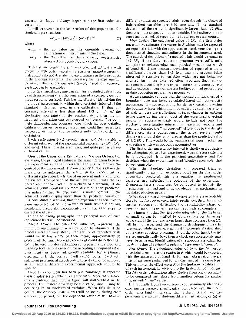
uncertainty, &r, N, is always larger than the first order un­certainty.

It will be shown in the last section of this paper that, for single sample situations:

5x,N=((5x,,ca l)2+(5x,.,)2)1/2 (7)

where

&K;,cai = the 2a value for the ensemble average of calibrations of instruments of this type,

8x:l = the 2a value for the stochastic uncertainties observed on repeated observations.

There is an immediate and very practical difficulty with executing Mh order uncertainty analysis: manufacturers of instruments do not describe the uncertainties in their products in the appropriate terms. It is necessary for the experimenter to assign the calibration uncertainty, based on whatever evidence can be assembled.

In critical situations, one can call for a detailed calibration of each instrument (i.e., the generation of a complete output-input response surface). This has the effect of identifying the individual instrument, to within the uncertainty interval of the standard instrument used in the calibration. If that un­certainty interval is less than about 1/3 or 1/4 of the stochastic uncertainty in the reading, 8x,j, then the in­strument calibration can be regarded as "certain." A com­plete data-reduction program, one which includes detailed calibration curves for every instrument, could then revert to a first-order estimator and be subject only to first order un­certainties.

Each replication level (zeroth, first, and Mh) yields a different estimator of the experimental uncertainty (8R0, 8R,, and 8RN). These have different uses, and quite properly have different values.

Uses of the Uncertainty Estimators of Various Orders. For every use, the principal feature is the same: iteration between the experiment and the uncertainty analysis to improve the control of the experiment. The uncertainty analysis allows the researcher to anticipate the scatter in the experiment, at different replication levels, based on present understanding of the system. Comparison of the achieved result with the ex­pected result then gives either a check or a warning. If the achieved results contain no more deviation than predicted, this indicates that the experiment is under control. If the achieved results display more than the predicted variation, this constitutes a warning that the experiment is sensitive to some uncontrolled or unobserved variable which is causing significant error; the experimenter can then take steps to correct the situation.

In the following paragraphs, the principal uses of each replication level will be discussed.

Zeroth Order. The calculated value 8R0 represents the minimum uncertainty in R which could be obtained. If the process were entirely steady, the results of repeated trials would lie within ± 5^0 of their mean, approximately 95 percent of the time. No real experiment could do better than 8R0. The zeroth order replication concept is mainly used as a planning tool, as one criterion for accepting a proposed set of instruments as being sufficiently readable for a planned experiment. If the desired result cannot be achieved with sufficient precision at zeroth order, then it cannot be achieved at all, and a different experimental approach should be selected.

Once an experiment has been put "on-line," if repeated trials display scatter which is significantly larger than ±8R0, this is evidence that there is significant unsteadiness in the process. The unsteadiness may be concealed, since it may be occurring in an unobserved variable. When this situation occurs, the observed instruments will be steady during each observation period, but the dependent variables will assume

different values on repeated trials, even though the observed independent variables are held constant. If the standard deviation of the results is significantly larger than 1/2 8R0, then one must suspect a hidden variable. Unsteadiness in this sense includes lack of repeatability in startup or reset control.

First Order: The calculated value of 8RU the first order uncertainty, estimates the scatter in R which must be expected on repeated trials with the apparatus at hand, considering the documented timewise unsteadiness in the instruments used. The standard deviations of repeated trials would be equal to 1/2 8R, if the data reduction program were sufficiently complete to acknowledge each physical mechanism which affected R. If the standard deviation of repeated trials is significantly larger than 1/2 8RU then the process being observed is sensitive to variables which are not being ac­counted for in the data reduction program. Such an oc­currence is a warning to the experimenter that diagnostic tests and development work on the test facility, control procedures, or data-reduction program are necessary.

As an example, suppose that the momentum thickness of a boundary layer was being calculated based only on velocity measurements — not accounting for density variations within the boundary layer which might be caused by small variations of wall temperature (reflecting, in turn, changes in ambient temperature during the conduct of the experiment). Actual results on successive trials would include not only the stochastic uncertainties inherent in measuring velocity and position, but also the "unrecorded" effects due to the density differences. As a consequence, the actual results would display a standard deviation greater than the predicted value of 1/2 8R{. This would be the warning that some mechanism was acting which was not being accounted for.

The first order uncertainty interval is chiefly useful during the debugging phase of an experiment, when the test system is being developed. It is the principal quantitative tool for deciding when the experiment is sufficiently repeatable, that is, well controlled.

When the standard deviation on repeated trials is significantly larger than expected, based on the first order uncertainty predicted, this is a warning that unobserved variables are affecting the outcome of the experiment. Diagnostic tests should then be conducted to identify the mechanism involved and to acknowledge that mechanism in the data-reduction program.

When the standard deviation of repeated trials is acceptably close to the first order uncertainty prediction, then there is no further evidence of difficulty; the repeatability phase of development of the experiment can be considered complete.

It is important that the first order intervals for the 8x{ be set as small as can be justified by observations on the actual apparatus. Ifthe&r, j are taken larger than necessary then 8R x

will be too large, and the diagnostic development may be terminated while the experiment is still incompletely described by its data-reduction program. If, on the other hand, the 8xt

are set unrealistically low, then a check on repeatability may never be achieved. Identification of the appropriate values for the &*:,, is thus the critical problem of experimental control.

Nth Order: The calculated value of 8RN, the Mth order uncertainty, estimates the scatter in R which could be expected with the apparatus at hand if, for each observation, every instrument were exchanged for another unit of the same type. This estimates the effect upon R of the (unknown) calibration of each instrument, in addition to the first-order component. The Mh order calculations allow studies from one experiment to be compared with those from another ostensibly similar one, or with " t rue" values.

If the results from two different (but nominally identical) experiments disagree significantly, compared with their Mh order uncertainty intervals, then either: (i) the two ex­periments are actually studying different situations, or (ii) at

Journal of Fluids Engineering JUNE 1982, Vol. 104/255

Downloaded 30 Aug 2010 to 139.82.149.123. Redistribution subject to ASME license or copyright; see http://www.asme.org/terms/Terms_Use.cfm

least one of the experiments is in error, Condition (i) might be generated, for example, by unmeasured differences in initial conditions of the experiment or unrecognized dependence of the process on some characteristic of the apparatus.

The Mh order uncertainty calculation must be used wherever the absolute accuracy of the experiment is to be discussed. First order will suffice to describe scatter on repeated trials, and will help in developing an experiment, but Mh order must be invoked whenever one experiment is to be compared with another, with computation, analysis, or with the "truth."

It frequently occurs that inclusion of all of the instrument calibration uncertainties yields such a large value for 8RN that the experiment seems doomed from the beginning. In such cases, the only recourse is to reduce the Mh order uncertainty intervals by detailed calibrations of the most critical in­struments. An important implication of equation (5) is that the uncertainties with large effect on the output are easy to identify, and should receive the most attention. At each stage of improvement, any term smaller than 1/4 of the largest term can usually be ignored. The same remark applies to calibration uncertainty, as indicated by equation (7).

When the predicted uncertainty interval 5RN has been reduced to an acceptable value, then the experiment may be tested against some known "true" values. If the experiment returns the " t rue" value within ±8RN, it may be considered qualified for data production. If not, then further develop­ment is indicated. There are few "true" values known. The principal sources of " truth" are those described as Basic Principles:

The Rate of Creation of Energy = 0

The Rate of Creation of + x Momentum = gcLF+x

The Rate of Creation of Mass = 0

The Rate of Creation of Entropy ^ —

Execution of a mass, momentum or energy balance on an apparatus, without knowledge of the expected Mh order uncertainty, is an essentially useless enterprise. To reach any conclusions, one must have the ability to assess the significance of the difference between the observed value and the expected value. The Mh order uncertainty analysis provides that ability.

In the absence of an applicable Basic Principle, one is frequently forced to use a secondary check: a baseline ex­periment. A baseline experiment is a data set which has so well stood the test of time that its validity is accepted by most workers in the field. Knowledge of the Mh order uncertainty intervals for both experiments is necessary before the significance of any difference between the observed and baseline values of R can be assessed.

Uncertainty Analysis on Computer-Based Data-Reduction Programs

It is impractical to execute an uncertainty analysis analytically for any but relatively simple cases. Complex data-reduction programs may involve many corrections to the data and use implicit forms or table look-ups or numerical in­tegration within the program. In such cases, the uncertainty-analysis program might be larger than the main program-certainly an unacceptable burden on the experimenter.

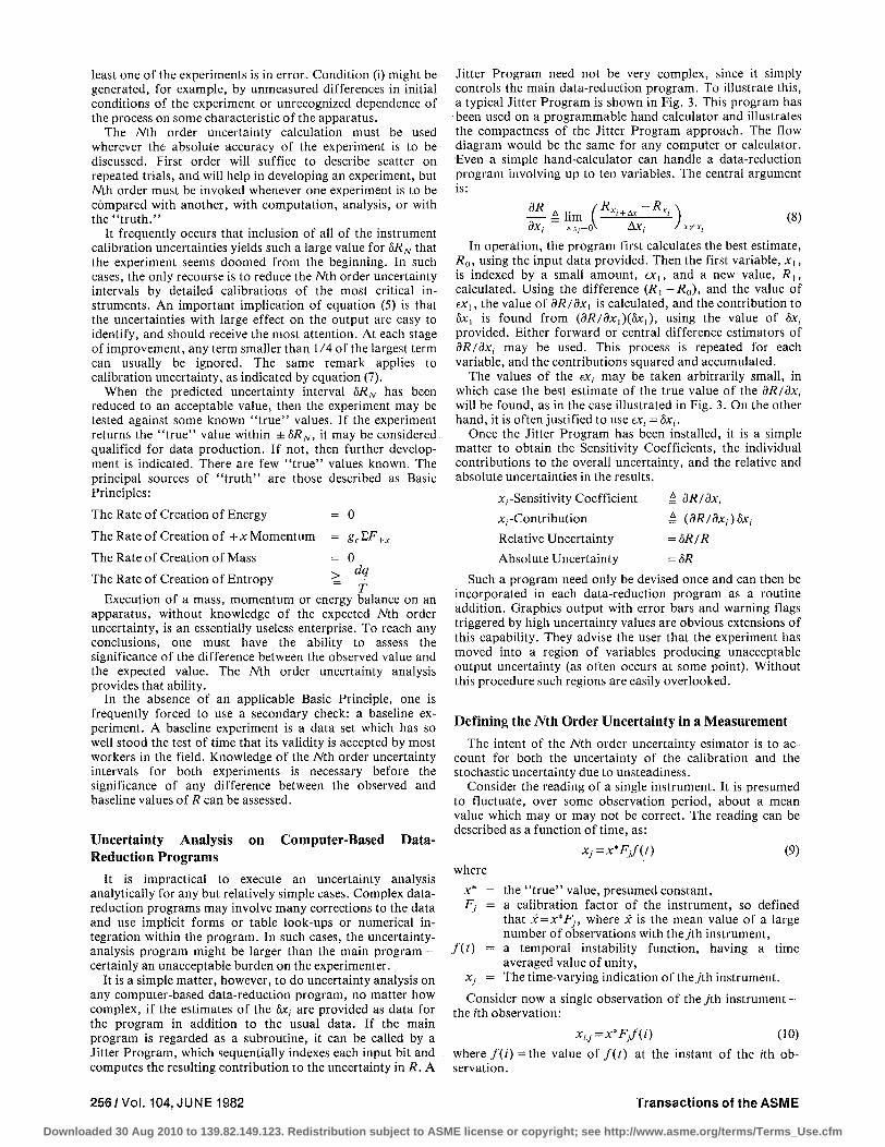
It is a simple matter, however, to do uncertainty analysis on any computer-based data-reduction program, no matter how complex, if the estimates of the Sx, are provided as data for the program in addition to the usual data. If the main program is regarded as a subroutine, it can be called by a Jitter Program, which sequentially indexes each input bit and computes the resulting contribution to the uncertainty in R. A

Jitter Program need not be very complex, since it simply controls the main data-reduction program. To illustrate this, a typical Jitter Program is shown in Fig. 3. This program has been used on a programmable hand calculator and illustrates the compactness of the Jitter Program approach. The flow diagram would be the same for any computer or calculator. Even a simple hand-calculator can handle a data-reduction program involving up to ten variables. The central argument is:

^ i h m (*«+*-*«) (8) ax, w,-o\ Axr, /***,-

In operation, the program first calculates the best estimate, R0, using the input data provided. Then the first variable, xx, is indexed by a small amount, exu and a new value, Rit

calculated. Using the difference (Rt -Ro), and the value of ex{, the value of dR/dxt is calculated, and the contribution to bxx is found from (dR/dx^bXi), using the value of 5x, provided. Either forward or central difference estimators of dR/dXj may be used. This process is repeated for each variable, and the contributions squared and accumulated.

The values of the ex, may be taken arbitrarily small, in which case the best estimate of the true value of the dR/dXj will be found, as in the case illustrated in Fig. 3. On the other hand, it is often justified to use ex, = &c,-.

Once the Jitter Program has been installed, it is a simple matter to obtain the Sensitivity Coefficients, the individual contributions to the overall uncertainty, and the relative and absolute uncertainties in the results.

x,-Sensitivity Coefficient = dR/dXj

^-Contribution = (dR/dx^SXj

Relative Uncertainty = 8R/R

Absolute Uncertainty = 8R

Such a program need only be devised once and can then be incorporated in each data-reduction program as a routine addition. Graphics output with error bars and warning flags triggered by high uncertainty values are obvious extensions of this capability. They advise the user that the experiment has moved into a region of variables producing unacceptable output uncertainty (as often occurs at some point). Without this procedure such regions are easily overlooked.

Defining the M h Order Uncertainty in a Measurement

The intent of the Mh order uncertainty esimator is to ac­count for both the uncertainty of the calibration and the stochastic uncertainty due to unsteadiness.

Consider the reading of a single instrument. It is presumed to fluctuate, over some observation period, about a mean value which may or may not be correct. The reading can be described as a function of time, as:

Xj=x*Fjf(t) (9)

where

x* = the " t rue" value, presumed constant, Fj = a calibration factor of the instrument, so defined

that x=x*Fj, where x is the mean value of a large number of observations with they'th instrument,

f(t) = a temporal instability function, having a time averaged value of unity,

Xj = The time-varying indication of they'th instrument.

Consider now a single observation of the y'th instrument -the z'th observation:

xiJ=x*FJf(i) (10)

where / ( / ) =±the value of f(t) at the instant of the fth ob­servation.

256/Vol. 104, JUNE 1982 Transactions of the ASME

Downloaded 30 Aug 2010 to 139.82.149.123. Redistribution subject to ASME license or copyright; see http://www.asme.org/terms/Terms_Use.cfm

The relative uncertainty in x,j can be written formally as:

It remains to show that this form has physical significance, and utility.

The functions Fj and / ( / ) can each be regarded as having a mean value which is 1.000, with normal distributions about this mean. Let 5F, and bf(t) equal twice the standard deviations of these functions. It can be safely assumed that instrument manufacturers describe the mean calibration of their instruments as well as possible, and that there is a normal distribution of the individual calibrations around the mean. It is also apparent that the observer will make every effort to record the mean value of a fluctuating sequence of values, so t h a t / ( O , an average, will have a value of 1.00.

If these assumptions are correct, then &F, stands for the uncertainty in calibration of the individual instrument used, and 5f(i) stands for the temporal component of the recording uncertainty.

Equation (11) thus accounts for the overall uncertainty in a single observation from a single instrument.

Rearranging and interpreting the terms shows the basis for the current treatment of the Mh order uncertainty estimate for single-sample experiments:

M(*4)!+(*«fr)2r dF

where x-,j —- = the uncertainty in the value of Xy caused by v/ the uncertainty in calibration SFj/Fy, i.e.,

Hf("\ °xucd' and xhJ —— = the uncertainty in the value of xLj caused by

*{1' the uncertainty in the temporal instability term; i.e., &cu .

This can be written as:

5xiJ=l(5xiiCal)2 + (8xi,1)

1}W2 (13)

Once again, it must be emphasized that &C/>cal is hard to identify. Most manufacturers are reluctant to describe their product in such terms, and frequently the experimenter must simply estimate this term, based upon experience or, at best, a few hints in the manufacturers' literature. As already suggested, use of such estimates is better than total lack of uncertainty analysis.

Applications for the Comparison of Experiment and Computation. Ideally, all the experimental results used as the basis for model formation and comparison to computation would be accompanied by reliable estimates of 8RN. In reality, this is not the case for most existing data sets, partly because of the difficulty, in the past, of doing the analysis for complex experimental programs. Given the methods of this paper, reliable estimates of &RN become feasible for future "record" experiments and are strongly recommended as a criterion for acceptance of such future "record" data.

When reliable estimates of 8RN are known, assessment of the degree of agreement between different data sets and between experiment and computation becomes both easier and more clear-cut. Two data sets "agree" when the data do not differ by more than the root-sum-square of the 8RN for the two experiments. The 8RN will in general be different for the two experiments, owing to different instruments and reduction programs; but when the two are roughly the same, disagreements larger than 1.4 8RN indicate some difference in the experiments, or the presence of an uncontrolled variable in one or the other experiment. When one 5RN is significantly larger than the other, disagreement beyond the larger value is the relevant test. These remarks apply point by point wherever the 5RN are known. For points where agreement is found, one

can conclude that the results are consistent, and that the presumed correct value does not differ from the mean of the two sets by more than the root-sum-square &RN for the two data sets.

When there are more than two data sets, the same principle can be extended. If, in a group of seven data sets, all the data lie within the uncertainty band found from the square-root of the sum-squares of the 5RN for all the sets, then a correlation band has been established. If two or three of the sets have smaller bRN than the others, and agree with each other within that uncertainty, a tighter correlation band can be formed.

Comparisons of computation with experiments could proceed on the assumption that differences between com­putation and experiment that exceed the value of 5RN for the data are attributable to approximations in either the model or the numerical procedure.

When only partial or rough estimates of the 8RN are known, the principles remain the same, but it becomes necessary to use judgment case by case.

Another use for the methodology of this paper is in ap­plication of criteria for evaluating data sets. As noted above, the data can be tested against known theory, as for example a check of the right- and left-hand side of the momentum in­tegral equation for shear layers. Since the measurement of some of the terms in the momentum equation typically have large uncertainties, it would be easy to conclude that the flows were three-dimensional, when in fact they were not. Specifically, disagreement by an amount less than the value of 6RN must be regarded as agreement, even though the disagreement might look large. The methodology of this paper can be applied to make such judgments both more specific and more meaningful than has been possible in the past.

Conclusion

Uncertainty analysis is a powerful diagnostic tool, useful during the planning and developmental phases of an ex­periment. Uncertainty analysis is also essential to rational evaluation of data sets, to comparison of more than one data set, and to checking computation against data.

There is no single value of uncertainty which is appropriate for all intended uses. The predicted uncertainty in a result R will depend upon the number of terms retained in the analysis, and this, in turn, is dependent on the end-use proposed for the uncertainty value.

The concept of "replication level" is introduced to aid in identifying which of the candidate terms should be retained in an uncertainty analysis.

Three conceptual levels of replication can be defined: Zeroth, first, and Mh order. These levels of replication admit of different sources of uncertainty: Zeroth Order: 8 Includes only interpolation uncertainty. 8 Useful chiefly during preliminary planning. First Order: 8 Includes unsteadiness effects, as well as interpolation. 9 Useful during the developmental phases of an experiment,

to assess the significance of scatter, and to determine when "control" of the experiment has been achieved.

Nth Order: 8 Includes instrument calibration uncertainty, as well as

unsteadiness and interpolation. 9 Useful for reporting results and assessing the significance

of differences between results from different experiment and between computation and experiment.

The basic combinatorial equation is the Root-Sum-Square:

. „ U &R \ 2 ( dR \ 2 ( dR \21W2

Journal of Fluids Engineering JUNE 1982, Vol. 104/257

Downloaded 30 Aug 2010 to 139.82.149.123. Redistribution subject to ASME license or copyright; see http://www.asme.org/terms/Terms_Use.cfm

The process is easily adapted to computer-based data reduction programs. A sequential jitter package can be written in standard form, which uses the existing data reduction program to execute the uncertainty analysis, ob­viating the need for a separate analysis. The additional computing time is usually not excessive.

Acknowledgments

' I appreciate very much the thoughtful and challenging conversations I have had on this subject with Steve Kline, of Stanford, and Bob Abernethy, of Pratt and Whitney Aircraft Co., over the past few years. Their grasp of the problem and willingness to discuss these ideas helped me find the language to put this work in context and, hopefully, express it more clearly than in earlier renditions. I would also like to thank Frank White, of the University of Rhode Island, for arranging the round-table discussion at the ASME Winter Annual Meeting which got all three of us together for a truly fruitful discussion.

D I S C U S S I O N

R. B. Dowdell1

There is a lot of uncertainty on uncertainty analysis but some analysis is better than no analysis at all. To the average engineer or experimenter, the principles set forth here and in the author's references may seem obscure and complex and too difficult to deal with. However, as the author ably points out, uncertainty analysis is an invaluable tool in the planning, development, interpretation and reporting of scientific and engineering tests and experiments. It should be a part of every accredited undergraduate engineering curriculum and taught with the same methodology and nomenclature. But how can this be done when we find such a wide discrepancy between the treatment in the authors paper and that in his references [4, 5, and 6].

This difference, of course, lies in the treatment of the bias or fixed errors. The author admits to the existence of such errors but contends that they can always be calibrated out or made negligibly small when compared to the random errors. The author's references [4, 5, and 6] carry along the bias errors throughout the analysis and then combine the bias and random errors for the final uncertainty figure. The actual method of combining these two types of errors is of no consequence since one has an estimate of each.

While the idea of reducing the fixed errors to a negligible size is certainly enticing, in the vast majority of engineering tests and experiments, it is not practical nor economical.

Certainly the economic side should be emphasized. In most cases it would be possible to reduce bias errors to a negligible amount if one were willing to spend the money and time to do so. This would usually require laboratory precision in­strumentation such as interferometers to measure length and oscillating crystals to measure time, and all the time that goes along with setting up and using such instrumentation.

In the majority of industrial experimentation and tests, and even in most university laboratories this is not the case. The instrumentation purchased is usually of an industrial quality and installed and operated within reasonable time constraints; dictated by economics. This type of instrumentation almost always has some bias or fixed errors and normally the procedures of installation and use can introduce additional bias.

Professor, Department of Mechanical Engineering, University of Rhode Island, Kingston, R. I. 02881.

References

1 Kline, S. J., and McClintock, F. A., "Describing Uncertainties in Single-Sample Experiments," Mechanical Engineering, Jan. 1953.

2 Schenck, Hilbert, Jr., Theories of Engineering Experimentation, McGraw-Hill, 1968.

3 Holman, J. P., Experimental Methods for Engineers, McGraw-Hill, 1966. 4 International Organization for Standardization (ISO) Standard ISO-5168,

"Measurement of Fluid Flow—Estimation of Uncertainty of a Flow Rate Measurement," ISO 5168-1978(e), p. 8.

5 ASME Committee MFFCC SCI, "Fluid Flow Measurement Uncertainty-Draft of 26 March, 1980," American Society of Mechanical Engineers, Codes and Standard Department, p. 14.

6 USAF AEDC-TR-73-5, "Handbook on Uncertainty in Gas-Turbine Measurements," AD 755356 (R. B. Abernethy et al.). Also available through the Instrument Society of America as "Measurement Uncertainty Handbook, Revised 1980," IS&N: 87664-483-3.

7 JANNAF, "ICRPG Handbook for Estimating the Uncertainty in Measurements Made with Liquid Propellant Rocket Engine Systems," CPIA Publication 180, AD 851127.

8 Kaarls, R., "Report of the BIPM Working Group on the Statement of Uncertainties," CIPM, Severes, France, Oct. 1980.

9 Thomas, H. A., in Marks Mechanical Engineers Handbook, Sixth Edition, Ch. 17, p. 26, McGraw-Hill (1964 printing, ed. T. Baumeister).

Thus an analysis of bias or fixed error is fundamental to any uncertainty estimate. I can find no fault in the author's treatment of random errors other than in the real world they would become mixed with bias errors.

I like the concept of his jitter program and plan to use it as soon as possible.

R. B. Abernethy2

Having reviewed drafts of this paper over several years, I am pleased and honored to have the opportunity to comment on it. Professor Moffat has made a considerable effort to describe his approach to uncertainty in a clear manner. He has removed much of my early confusion about his techniques. I appreciate the hours we have spent together discussing our disagreements and agreements. I would like to use this discussion to briefly describe my conclusions, opinions and remaining areas of disagreement.

There is currently an enormous effort to arrive at a single, simple uncertainty methodology. For those of us that have argued the issues for decades, it seems like a miracle that suddenly we have a number of national and international standards near approval that share a single, simple methodology. These include ASME [5] and [9], S.A.E. [11], ISO [20]. These draft standards are updated versions of earlier documents, ISA [18], USAF [6], and JANNAF [7]. I am sorry that Professor Moffat's approach is not consistent with this methodology although he has made an effort to bridge the g"p. However, Professor Moffat and I believe that given the same experiment, our uncertainty analyses would produce the same result.

I strongly endorse Professor Moffat (and Professor Kline's) plea for more pretest uncertainty analysis. This allows for corrective action to reduce unacceptable errors before the test. This is a major point in Professor Moffat's paper.

The "zero order to Mh order replication" of experiments initially confused me. As I understand it now, this is an ap­proach to identify and estimate all the sources of elemental errors. I believe it is more complex than the approaches described in the methodology we endorse, but it certainly emphasizes the need for a complete identification of all errors. Statisticians would use an analysis of variance to

2 Pratt & Whitney Aircraft, West Palm Beach, Fla. 33402. Mem. ASME.

258/Vol. 104, JUNE 1982 Transactions of the ASME

Downloaded 30 Aug 2010 to 139.82.149.123. Redistribution subject to ASME license or copyright; see http://www.asme.org/terms/Terms_Use.cfm