arX

iv:1

504.

0591

7v1

[qu

ant-

ph]

22

Apr

201

5

Departament d’Optica, Facultat de Fısica

Contributions

to the Quantum Optics of

Multi–mode Optical Parametric Oscillators

PhD dissertation by

Carlos Navarrete–Benlloch

Under the supervision of

Eugenio Roldan Serrano

and

German J. de Valcarcel Gonzalvo

Valencia, Spain; December, 2011

AGRADECIMIENTOS [ACKNOWLEDGEMENTS]

Escribir los agradecimientos de esta tesis genera en mı una doble sensacion de felicidad. El primer motivo es obvio:ello significa que el final de este largo (pero bonito) camino que ha supuesto redactar tan pensado documento estallegando a su fin, lo cual no es poco, ya que meses atras me parecıa que el camino era infinito (tras escribir cadaapartado, siempre tenıa la sensacion de que habıa algo mas que decir, algo mas sobre lo que incidir, algo mas quematizar... la paradoja de Zenon parecıa mas real que nunca). Sin embargo, la mayor parte de la alegrıa que suponeescribir estos agradecimientos viene de otro sitio: pensar en a quien agradecer y como, me hace recordar el caminoexacto que me ha llevado a este punto, recordar a las personas y los momentos que han supuesto (en mayor o menormedida) puntos de inflexion en mi vida, que me han ayudado a elegir que direccion tomar en cada bifurcacion; y claro,teniendo en cuenta lo contento que me ha hecho la fısica y lo que le rodea desde que entre en la universidad, recordartales cosas no puede suponer mas que una tremenda alegrıa.

En este sentido, sin duda son mis padres los primeros a los que debo mi agradecimiento (tanto cronologicamente,fueron los primeros que estuvieron ahı para mı, como cuantitativamente). Corren tiempos en los que siento quela economıa es el motor fundamental de la mayor parte de la gente, tiempos en los que estamos constantementebombardeados con la idea de que el camino a la felicidad es acumular dinero (y poder, a ser posible); pero tambiensiento que he conseguido desligarme de tal “movimiento”, que he conseguido encontrar dos cosas en la vida, la cienciay la musica, de las cuales puedo plantearme vivir, a la vez que sentirme feliz y realizado haciendolas. Pues bien,puedo decir con total certeza que tal logro es fruto de los valores que mis padres me han inculcado desde pequeno.Ellos siempre me han proporcionado todos los medios que estuvieran a su alcance y todo el apoyo posible para haceraquello que quisiera, eso sı, siempre que consiguiera convencerles de dos cosas: que lo harıa esforzandome al maximode verdad, y, sobre todo, que lo harıa unicamente mientras me hiciera realmente feliz; las palabras dinero, futuro, otriunfo, no estaban en su discurso.

Quizas quien mas ha “sufrido” mi faceta de cientıfico es Susana, mi novia, companera de andanzas en la vida, ymayor inspiracion durante los ultimos 8 anos. No puedo mas que agradecerle la paciencia infinita que tiene conmigo;del futuro solo espero que las cosas buenas que conllevan compartir la vida con un cientıfico–musico superen comohasta ahora la inestabilidad y las incomodidades (vida en el extranjero, noches y fines de semana de trabajo, etc...)intrınsecas a dicho “tıtulo”. Bien sabes que “te vull” aunque a veces no te lo diga lo suficiente.

En lo que a la parte cientıfica se refiere, no cabe ninguna duda de que a quien mas tengo que agradecer es amis directores Eugenio y German; desde el principio (y hablamos de antes de terminar la carrera de Fısica) mehicieron sentir como un colaborador mas con el potencial de aportar buenas ideas a la investigacion que estuviesemosdesarrollando, a la vez que pusieron a mi disposicion todos los medios posibles para transferirme toda la fısica quealmacenan (que no es poca). Pero mas alla de lo puramente cientıfico, me siento orgulloso de que me hayan dejadoentrar en sus vidas hasta el punto de haberse convertido en dos de las personas que mas aprecio y en las que mas meapoyo a dıa de hoy. Desde luego, Eugenio y German, no aspiro mas que a convertirme el dıa de manana en alguientan digno y merecedor de carino, respeto y admiracion como vosotros.

Hay gente que piensa que por ser hijo unico no tengo hermanos, pero de una de las cosas que mas orgulloso mesiento es de haber demostrado que dicha gente se equivoca: Apa, Pabl, Fons, Alberto y Rika son prueba de ello. Apa yPabl han estado ahı casi desde que puedo recordar; juntos hemos pasado por casi todo lo que se puede pasar, y hemossobrevivido! Mi vida sin Fons, ciertamente habrıa sido completamente distinta; a el no le debo unicamente su amistadtotalmente desinteresada, sino tambien el haberme abierto musicalmente, y con ello haber contribuido radicalmente aque mi vida sea como es ahora. Alberto es el que mas tardo en llegar a mi vida, pero se ha convertido en quien mejorentiende esta faceta tan importante de mi vida que es la ciencia; no conozco persona mas sincera y falta de maldad oegoısmo (vale, quiza Fons!), por lo cual tiene mi mas sincera admiracion. Rika fue mi pilar basico durante los primerosanos de carrera, los cuales dudo que hubieran sido tan productivos y realizadores sin su presencia; solo puedo darlelas gracias por esos anos que vivimos juntos, y decirle cuanto echo de menos la sensacion de tenerle a mi (y estar asu) lado.

iv Agradecimientos [Acknowledgements]

Me siento muy afortunado de contar con una familia que siempre me hace sentir especial, a la vez que me pone lospies en la tierra (lo cual no es sencillo trabajando en cosas tan abstractas como la Fısica Teorica, o tan intensas comola Musica). Siento que una parte de cada uno vosotros esta en mi interior, tanto de los que me han criado: mi AbueloManolo, mi Yaya Lola, mi Tıa Loles, y mis Tıos Pepa y Chani; como de con los que me he criado: mi Teta Jose ymis Primos Rafa, Patricia, Dani y Carola. No me gustarıa olvidarme tampoco de los nuevos miembros de la familiaque han ido apareciendo con el tiempo: mis sobrinitos Pablo y Alicia, y mis “cunaos” Paco, Sergi, Vicky, y Silvia; nitampoco de mis “tıos y primos postizos”, en especial de mi tıa Jose y mi tıo Pedro, que tan buenas palabras guardansiempre para mı.

Tambien me gustarıa agradecer a mi “familia por extension”, la familia de Su, a la cual tengo muy presente cadadıa y considero una parte muy relevante de mi vida. Muchas gracias a “Los Mayores” (Paloma, Carlos y Amparo) ya “Los Jovenes” (Emi, Moni, y Mir), por abrirme las puertas de sus vidas sin trabas (bueno, aunque a Mir le costoun poco mas que los demas... jejeje).

Me es imposible trazar la trayectoria que me ha llevado a este momento sin recordar a todos los profesores queme han influenciado e inspirado a lo largo de mi vida. Dentro de estos, quizas los mas importantes, porque sin ellosdudo que me hubiese dado cuenta de que la Fısica y las Matematicas son mi vocacion, son mis profesores del instituto(del “cole”, como nosotros lo llamamos). Encarna Giner fue sin duda la que mas me abrio los ojos y a la que con mascarino recuerdo; cuando menos lo esperaba, ella me mostro lo bonitas que pueden llegar a ser las matematicas, y medejo maravillado tras hacerme entender que solo requieren de comprenderlas (y no de memorizarlas) para utilizarlase interiorizarlas. Mi mayor suerte fue su formacion en Fısica Teorica (a la que yo finalmente me he dedicado), yaque le permitio introducirme en el mundo de la Relatividad General y la Geometrıa Diferencial hacia el final denuestro tiempo juntos. Chencho Pascual, mi gran profesor de Fısica, fue el primer profesor que nos planteo preguntasinteresantes, con animo real de que fueramos nosotros, los estudiantes, los que encontraramos las respuestas; cuandocreıa que las Matematicas eran mi vocacion, el me hizo ver que la Fısica es precisamente la aplicacion de estas almundo real, la forma en que preguntamos a la naturaleza para obtener respuestas a las preguntas mas fundamentales,y con ello me hizo encontrar mi vocacion real, la Fısica Teorica. Siendo cientıfico, quizas algo mas sorprendente es elhecho de que cuando pienso en los profesores que mas me motivaron en dicha epoca, mi profesor de Lengua Castellana,Angel Umbert, sea de los primeros que me viene a la cabeza; gracias a el tambien, aunque no sepa verbalizar muybien porque exactamente (al margen de que fuera, sin duda, uno de los mejores profesores que he tenido nunca).

Durante mi ultimo ano de instituto tuve la suerte de participar en la Olimpiada de Fısica, lo cual me permitio recibir“clases avanzadas” de Fısica de mano de varios profesores de la Universitat de Valencia y la Universidad Politecnica deValencia. La experiencia fue inolvidable, y no puedo mas que agradecer a dichos profesores su entrega desinteresadaque tanto me motivo a coger el camino de la Fısica finalmente con el fin de seguir aprendiendo y convertirme en undocente como ellos algun dıa. Guardo especial carino a Fernando Tena, que se encargo de “cuidar” a los olımpicosvalencianos durante la fase espanola, y que fue quien mas me inspiro durante todas las fases, ası como a Amparo Pons,Jose Luis Cruz, Miguel Andres y Paco Pomer.

La carrera de Fısica cumplio sobradamente con mis expectativas en lo que a disfrutar aprendiendo se refiere; anosatras nunca hubiese pensado que una “actividad intelectual” podrıa llenarme y motivarme tanto. No obstante, estono hubiese sido posible sin el esfuerzo de algunos profesores a los que ahora me gustarıa agradecer explıcitamente:Jose Marıa Ibanez (Calculo y Evolucion Estelar), Jose Marıa Martı (Algebra y Dinamica de Fluıdos), Ramon Cases(Lab. Fısica General y Fısica Nuclear y de Partıculas), Jose Luis Cruz (Fısica General y Ondas Electromagneticas),Domingo Martınez (Fısica General y Lab. Electromagnetismo), Eugenio Roldan (Fısica General, Optica Cuanticay Optica No lineal), Albert Ferrando (Fısica General), Pas Garcıa (Optica Geometrica y Procesos Estocasticos enFotonica), Carlos Ferreira (Optica Geometrica), Julio Pellicer (Termodinamica), Chantal Ferrer (Mecanica y Ondas),Jon Marcaide (Astronomıa y Astrofısica), Juan Zuniga (Metodos Numericos), Juan Carlos Soriano (Optica y Pro-cesos Estocasticos en Fotonica), Jose Marıa Isidro (Fısica Cuantica), Vicente Munoz (Electromagnetismo), JuanfranSanchez (Electromagnetismo), Kiko Botella (Lab. Fısica Cuantica y Mecanica Cuantica Avanzada), Pepe NavarroSalas (Geometrıa Diferencial, Variedades y Topologıa, y Teorıa Cuantica de Campos en Espacios Curvos), Benito Gi-meno (Electrodinamica), Nuria Rius (Mecanica Teorica y Teorıa Cuantica de Campos a Temperatura Finita), ManuelVicente Vacas (Mecanica Cuantica), Miguel Andres (Ondas Electromagneticas), Vladimir Garcıa (Fısica Estadıstica),German de Valcarcel (Optica Cuantica y Optica No Lineal), Fernando Silva (Optica Cuantica), Ramon Lapiedra(Relatividad General y Cosmologıa), Toni Pich (Teorıa Cuantica de Campos y Cromodinamica Cuantica), JavierGarcıa (Procesos Estocasticos en Fotonica), Pepe Bernabeu (Teorıa Electrodebil), Vicent Gimenez (Teorıa Cuanticade Campos en el Retıculo), ası como a Armando Perez y Arcadi Santamaria, a Pedro Fernandez y Javier Urcheguıa(ambos de la Universidad Politecnica de Valencia), y a Juan Leon (del Instituto de Fısica Fundamental del CSIC enMadrid), que, aunque no me dieron clase, contribuyeron a mis ganas de iniciar la carrera investigadora. Por razonesobvias de espacio, me es imposible explicar los motivos concretos por los cuales cada uno de estos profesores puso su

v

granito de arena (o saco de arena en muchos casos) para convertirme en el investigador que soy hoy en dıa, pero estoyseguro de que la mayorıa de ellos conocen perfectamente sus contribuciones particulares.

Por otro lado, uno siempre empieza la universidad con un poco de nerviosismo, sobre todo porque nunca sabe conque tipo de gente se va a encontrar en clase (especialmente alguien como yo, que estudio todos los cursos anteriores enel mismo centro, con lo cual no hizo el cambio del “colegio” al “instituto”). Por suerte, gran parte de la culpa de quesienta que la carrera de Fısica me lleno tanto la tienen precisamente los companeros con los que comence a estudiarla:Rika, Ave, Bego, Diana, Javi (Alicante), Javi (Aragorn), Susana, Carlos, Raul y Vıctor, son a los que mas carinotengo, sobre todo porque son con los que mas contacto sigo teniendo (aunque no me olvido de Juan, Marıa Luisa yAli!). Algo mas tarde (hacia tercero), llegaron otros companeros a los que tambien aprecio mucho: Alberto, Davidy Sergio; y algo mas tarde aun, ya en la epoca del doctorado, conocı a Zahara e Isa, que me han ayudado de variasformas en la recta final del doctorado. Me alegro de que supieramos ver que el camino correcto era el de compartir yayudarnos los unos a los otros tanto como pudieramos (algo que parece trivial, pero que no muchas clases hacen); noes casualidad que no sean pocos los profesores que afirman que hemos sido “el curso mas gratificante que han dado”,gracias y enhorabuena companeros!

2006 fue un ano muy especial: es el ano en el que termine la carrera, a la vez que aprendıa los fundamentos de laBiologıa Molecular y la Ingenierıa Genetica a traves de mi participacion en el proyecto iGEM. Aprender esas ramas dela Biologıa es algo que llevaba anos queriendo hacer, pero que nunca pense que podrıa realizar de verdad, y me gustarıaagradecer en especial a Arnau, Emilio, Alberto, Cate, Chevi, Gus, Carlos, Cris, Diana, Minerva, Albert, Pedro, Javi yJesus, por haber generado el ambiente cientıfico y humano perfecto para desarrollar tal labor. Nunca olvidare el anoque pasamos juntos y las experiencias que vivimos (tanto nuestros primeros congresos cientıficos —en MIT ni masni menos, eso sı fue “colarse” en el mundo de la investigacion por la puerta grande—, como las carreras de sillas enel laboratorio); mi tiempo con vosotros es con lo que comparo cualquier otro momento de mi carrera investigadoracuando quiero saber si de verdad estoy siendo feliz en lo que hago, no se puede ir con mas ilusion a un laboratorio decon la que iba en aquella epoca.

Quiero agradecer tambien a los miembros del grupo de Optica Cuantica y No Lineal en el que trabajo, tanto alos presentes como a los pasados, por haberme hecho sentir en un ambiente inmejorable durante mi doctorado; mealegra poder llamar “amigos” a la mayorıa de ellos. Muchas gracias en especial a Fernando Silva, que siempre meayuda con todas sus fuerzas en cada mınima cosa que necesito; quiero que sepa que considero que, junto a Alberto yFons (ver arriba), es la persona con menos maldad que conozco. Muchas gracias tambien por su inmejorable actituda los companeros con los que he colaborado en el grupo: Ferran Garcia (con quien comparto algunas ideas de estatesis), Robert Hoppner (pese a que no consiguieramos hacer llegar a buen puerto nuestras ideas), Alejandro Romanelli(sin el cual no creo que hubiese hecho la parte numerica de la tesis nunca) y Joaquın Ruiz–Rivas (con quien acabode comenzar, pero con quien ya he compartido unas cuantas alegrıas!); me he encontrado muy a gusto trabajandocon vosotros. No me olvido de Amparo Docavo, la persona que hace que las tareas administrativas que tan mal seme dan parezcan sencillas; gracias por tener siempre una sonrisa en la cara cuando hablamos. Isabel Perez fue laestudiante de doctorado que allano el camino hacia la Optica Cuantica (la de verdad, no esa con el campo clasico,jiji) en el grupo, de forma que yo ya pude tomar el relevo con “el chip cambiado”; le agradezco que me haya tratadodesde que estaba en la carrera como un amigo, y, en lo que a esta tesis se refiere, que se haya tomado la “molestia” deevaluarla (nadie mejor para hacerlo, por otro lado). Agradezco tambien a Vıctor Sanchez por tantas conversacionesinteresantes que hemos tenido sobre ciencia y lo que la rodea, y a Kestutis Staliunas por ayudarme siempre que lohe necesitado. Hago extensivos estos agradecimientos al resto de gente con la que he tenido el placer de coincidir delos grupos de Gandıa (Vıctor Espinosa, Javier Redondo, Ruben Pico, Paco Camarena, Joan Martınez,...) y Terrasa(Crina Cojocaru, Ramon Herrero, Josep Font, Lina Maigyte,...). Por ultimo, me gustarıa dar las gracias y transmitirtodo mi carino a Ramon Corbalan y Ramon Vilaseca (Los Ramones!), cuya personalidad me inspira y tomo comomodelo, por haber dejado a mi alrededor a tantos “hijos cientıficos de calidad” que tambien son algunas de las mejorespersonas que conozco.

Everyone who knows me knows that I’ve never been much of a traveller, especially when it is for touristic reasons;however, at a very early stage of my PhD I came to realize that travelling for scientific reasons (such as congresses orvisits to research groups) is actually quite rewarding at many levels. I would have never grown to be the scientist that Iam without the experiences that I’ve lived and the people that I’ve met during these “scientific travels”. In this sense,I would like to first thank Ignacio Cirac, Peter Drummond, Jeff Shapiro, and Nicolas Cerf for allowing me to becomea “temporary member” of their research groups, and for treating me like a fellow researcher, giving me all the toolsneeded to become productive under their watch. As a PhD student it is easier to hear the not–so–nice stories about

vi Agradecimientos [Acknowledgements]

the behaviour of top researchers than the nice ones, and meeting them has been one of the most inspiring experienceson this regard, as now I know that one can be at the very top of science without compromising his kindness andintegrity.

On the other hand, if I have been any productive at all during my visits to foreign research centres, it is becauseI’ve been lucky enough to collaborate with some of the nicest people that I have ever met, and who of course I considernow my friends. I owe so much to Ines de Vega and Diego Porras, my very first collaborators (together with Ignacio)outside the shelter of my research group and my usual research area; thanks for treating me so well and have confidencein me. Fate decided that I should meet Raul Garcıa–Patron at the best possible time, and, by his hand, Nicolas Cerf.Both Raul and Nicolas came as a blessing during my visit to MIT, inviting me to collaborate on a very interestingtopic, and giving me all the chances to offer my opinions and ideas concerning it, even though they knew that I neverworked on pure quantum information before. Finally on this list of collaborators are my dearest friends GiuseppePatera and Chiara Molinelli; I am so glad that we are finally collaborating on something altogether, I am sure thatmany happy memories will born from this collaboration!

Living in a new city and working in a new environment and topic can be a little bit overwhelming; however,if I didn’t get any anxious in my three–months visits to Munich, Melbourne, and Boston it is in part because ofthe amazing people that I met there. I would like to thank many people for making me feel welcome and “part ofsomething” during these visits. At the MPQ, my officemates (Heike Schwager, Philipp Hauke, and Christine Muschik),“the Spanish crowd” (apart from Diego and Ines, Mari Carmen Banuls, Maria Eckholt, Miguel Aguado, Lucas Lamata,and Oriol Romero), Veronika Lechner (always a ray of sunshine in the cold Munich!), Geza Giedke (pure kindness),Albert Schliesser (oh my god! an experimentalist on this list!), as well as David Novoa, Christina Krauss, Mikel Sanz,Sebastien Perseguers, Eric Kessler, Fernando Patawski, Matteo Rizzi, and Maarten van den Nest. In Melbourne I hadthe best housemate possible, Simon Gorman, an amazing musician (animateur!), father of the two sweetest/craziestlittle blondies in the world (Scarlett and Sapphire) and with the coolest sister (Rachel!); I also had the chance to meetsome of the best musicians that I know, such as Chris Hale or Gian Slater (thanks to Esther for hooking me up withChris!). The working environment at the ACQAO in Swinburne University was excellent thanks to Tim Vaughan,Margaret Reid, Qionyi He, Peter Hannaford, Xia–Ji Liu, Hui Hu, and the kind Tatiana Tchernova, who helped mewith the administrative issues. I had the chance to start writing this dissertation while living halfway between Harvardand MIT, what was actually an incredibly inspiring experience, highly amplified by spending lots and lots of time withmy dear friend David Adjiashvili in the many restaurants that the area has to offer, and specially at “our office”, theAtomic Bean Cafe, with the best waitress ever, Sam! I also thank Chelsea Martınez, my “orientation friend” MarıaRamırez, my officemate Niv Chandrassekaran, and the Quantum Girls (Veronika Stelmakh, Valentina Schettini, andMaria Tengner), for being such a wonderful people.

Una parte muy importante de mi vida durante los ultimos 12 anos ha sido la musica. Al primero que debo miagradecimiento en este sentido es a Pabl, mi “pareja musical”, con quien he compartido todos y cada uno de losproyectos en los que he participado. Guardo ademas mucho carino hacia la gente con la que Pabl y yo formamosnuestra primera banda, Desyrius, especialmente a Vero, Fran y Jose Angel, ası como a la gente de nuestra segundabanda, Fuego Fatuo (Hada, Empar y Vicent son lo que recuerdo mas vıvidamente), la cual nos permitio dar el saltohacia el proyecto totalmente instrumental y abierto a cualquier estilo musical en el que llevamos trabajando ya 7 anos,Versus Five. Mis agradecimientos a los miembros originales de Vs5 (Borja, Diego y Dani), por poner tanta ilusion enun proyecto a priori tan “friki”, y hacer con ello que empezara a funcionar. Tambien a la gente que ha ido dejandosu huella en este proyecto tan gratificante a nivel personal (Moli, Marcos, Luis y Raul) y a los companeros del restode bandas de Valencia con las que hemos interaccionado (Vahladian, “los Groovers”, y Non Essential en especial).Y, sobre todo, muchas gracias a la gente que ha participado en la banda en los ultimos tiempos: los Versus (Riki,Osvaldo, Xavi, Javi, Vıctor y —por poco no llegas a esta lista de agradecimientos— David!), los “crew” (Apa, Alberto,Rika, Ferrandiz y Fons), los ingenieros (Jorge y Alberto), los disenadores (Juanma e Isma) y las colaboraciones (Voroy David).

El final de mi doctorado ha sido (y en parte sigue siendo) un momento de relativa ansiedad, sobre todo por laincertidumbre acerca de lo que vendra luego, y la perspectiva de un cambio obligatorio respecto a una situacion en laque me siento muy comodo y feliz. No obstante, hay un par de “tareas periodicas” que me han ayudado a llevar mejoresta situacion: el fronton y las “cenas de los miercoles”. Quiero agradecer a la gente con la que juego o he jugado afronton estos ultimos dos anos (aproximadamente), especialmente a Alberto, Rafa, Antonio (mi companero!), Joaquın,Juan, Pablo, Manu y los Joses; mucha de la ansiedad que siento se va en cada raquetazo y en cada conversacion quemantenemos. Igualmente, agradezco a la gente de las cenas de los miercoles, en especial a Cyn, Paty, Carlos, Gonzalo,Belen, Sergio, Amparo y Ana; no sabeis cuanto me hacen olvidar la ansiedad de la que hablaba las risas que nospegamos.

vii

Finalmente, muchas gracias a Alfredo Luis (un sol!), Giuseppe Patera, Isabel Perez, Alberto Aparici, y mis direc-tores por haberse tomado el tiempo de corregir mi tesis, ası como a Antonio Garrido, que ha puesto tanto esfuerzo enla edicion (impresion y encuadernacion) de esta tesis.

En definitiva, muchas gracias a todos los que habeis contribuido en mayor o menor medida a que llegue hasta elpunto en el que me encuentro ahora; se que me arriesgado mucho al confeccionar una lista tan especıfica, ya que,teniendo en cuenta el poco tiempo que he tenido para hacerla, la probabilidad de que haya olvidado a alguien es alta.Aun ası, me gustarıa que se entendiera este esfuerzo como una muestra real de mi gratitud, y si alguien siente que “lehe olvidado”, tan solo decirle que probablemente tenga razon y que no se lo tome a mal: lo he intentado!

Un abrazo a todos!

Carlos.

viii Agradecimientos [Acknowledgements]

CONTENTS

Agradecimientos [Acknowledgements] . . . . . . . . . . . . . . . . . . . . . . . . . . . . . . . . . . . . . . . . . . . iii

1. Introduction . . . . . . . . . . . . . . . . . . . . . . . . . . . . . . . . . . . . . . . . . . . . . . . . . . . . . . 11.1 Squeezed states of light: Generation and applications . . . . . . . . . . . . . . . . . . . . . . . . . . . . 11.2 Overview of the thesis . . . . . . . . . . . . . . . . . . . . . . . . . . . . . . . . . . . . . . . . . . . . . 1

1.2.1 The quantum optics behind squeezing, entanglement, and OPOs. . . . . . . . . . . . . . . . . . 11.2.2 Original results: New phenomena in multi–mode OPOs. . . . . . . . . . . . . . . . . . . . . . . 4

2. The quantum harmonic oscillator . . . . . . . . . . . . . . . . . . . . . . . . . . . . . . . . . . . . . . . . . . 72.1 Classical analysis of the harmonic oscillator . . . . . . . . . . . . . . . . . . . . . . . . . . . . . . . . . 72.2 Hilbert space of the harmonic oscillator and number states . . . . . . . . . . . . . . . . . . . . . . . . 82.3 Coherent states . . . . . . . . . . . . . . . . . . . . . . . . . . . . . . . . . . . . . . . . . . . . . . . . . 10

2.3.1 Connection to classical mechanics . . . . . . . . . . . . . . . . . . . . . . . . . . . . . . . . . . . 102.3.2 Properties of the coherent states . . . . . . . . . . . . . . . . . . . . . . . . . . . . . . . . . . . 112.3.3 Phase space sketch of coherent states . . . . . . . . . . . . . . . . . . . . . . . . . . . . . . . . . 13

2.4 Squeezed states . . . . . . . . . . . . . . . . . . . . . . . . . . . . . . . . . . . . . . . . . . . . . . . . . 142.4.1 Definition and relevance . . . . . . . . . . . . . . . . . . . . . . . . . . . . . . . . . . . . . . . . 142.4.2 Minimum uncertainty squeezed states . . . . . . . . . . . . . . . . . . . . . . . . . . . . . . . . 15

2.5 Entangled states . . . . . . . . . . . . . . . . . . . . . . . . . . . . . . . . . . . . . . . . . . . . . . . . 162.5.1 The EPR argument and quantum non-locality . . . . . . . . . . . . . . . . . . . . . . . . . . . 162.5.2 Entanglement and the two–mode squeezing operator . . . . . . . . . . . . . . . . . . . . . . . . 172.5.3 Enhancing entanglement by addition and subtraction of excitations . . . . . . . . . . . . . . . . 19

2.6 The harmonic oscillator in phase space . . . . . . . . . . . . . . . . . . . . . . . . . . . . . . . . . . . . 212.6.1 Phase space distributions . . . . . . . . . . . . . . . . . . . . . . . . . . . . . . . . . . . . . . . 212.6.2 The positive P distribution . . . . . . . . . . . . . . . . . . . . . . . . . . . . . . . . . . . . . . 232.6.3 Fokker–Planck and stochastic Langevin equations . . . . . . . . . . . . . . . . . . . . . . . . . . 24

3. Quantization of the electromagnetic field in an optical cavity . . . . . . . . . . . . . . . . . . . . . . . . . . 273.1 Light as an electromagnetic wave . . . . . . . . . . . . . . . . . . . . . . . . . . . . . . . . . . . . . . . 273.2 Quantization in free space: Plane waves and polarization . . . . . . . . . . . . . . . . . . . . . . . . . . 28

3.2.1 Quantization in terms of plane waves . . . . . . . . . . . . . . . . . . . . . . . . . . . . . . . . . 283.2.2 Vector character of the fields and polarization . . . . . . . . . . . . . . . . . . . . . . . . . . . . 30

3.3 Paraxial optics and transverse modes . . . . . . . . . . . . . . . . . . . . . . . . . . . . . . . . . . . . . 323.3.1 Optical beams and the paraxial approximation . . . . . . . . . . . . . . . . . . . . . . . . . . . 323.3.2 Transverse modes . . . . . . . . . . . . . . . . . . . . . . . . . . . . . . . . . . . . . . . . . . . . 33

3.4 Quantization in an optical cavity . . . . . . . . . . . . . . . . . . . . . . . . . . . . . . . . . . . . . . . 373.4.1 Geometrical optics: Propagation through optical elements and stable optical cavities . . . . . . 373.4.2 Considerations at a non-reflecting interface . . . . . . . . . . . . . . . . . . . . . . . . . . . . . 393.4.3 Modes of an optical resonator . . . . . . . . . . . . . . . . . . . . . . . . . . . . . . . . . . . . . 403.4.4 Quantization of the electromagnetic field inside a cavity . . . . . . . . . . . . . . . . . . . . . . 43

4. Quantum theory of open cavities . . . . . . . . . . . . . . . . . . . . . . . . . . . . . . . . . . . . . . . . . . 454.1 The open cavity model . . . . . . . . . . . . . . . . . . . . . . . . . . . . . . . . . . . . . . . . . . . . . 454.2 Heisenberg picture approach: The quantum Langevin equation . . . . . . . . . . . . . . . . . . . . . . 464.3 Schrodinger picture approach: The master equation . . . . . . . . . . . . . . . . . . . . . . . . . . . . 474.4 Relation of the model parameters to physical parameters . . . . . . . . . . . . . . . . . . . . . . . . . . 494.5 Quantum–optical phenomena with optical lattices . . . . . . . . . . . . . . . . . . . . . . . . . . . . . 50

4.5.1 The basic idea . . . . . . . . . . . . . . . . . . . . . . . . . . . . . . . . . . . . . . . . . . . . . 51

x Contents

4.5.2 Superradiant phenomenology . . . . . . . . . . . . . . . . . . . . . . . . . . . . . . . . . . . . . 53

5. Detection of the output field . . . . . . . . . . . . . . . . . . . . . . . . . . . . . . . . . . . . . . . . . . . . 595.1 The output field . . . . . . . . . . . . . . . . . . . . . . . . . . . . . . . . . . . . . . . . . . . . . . . . 595.2 Ideal detection: An intuitive picture of photo- and homodyne detection . . . . . . . . . . . . . . . . . 605.3 Real photodetection: The photocurrent and its power spectrum . . . . . . . . . . . . . . . . . . . . . . 625.4 Real homodyne detection: Squeezing and the noise spectrum . . . . . . . . . . . . . . . . . . . . . . . 65

6. Quantum description and basic properties of OPOs . . . . . . . . . . . . . . . . . . . . . . . . . . . . . . . . 696.1 Dielectric media and nonlinear optics . . . . . . . . . . . . . . . . . . . . . . . . . . . . . . . . . . . . . 69

6.1.1 Linear dielectrics and the refractive index . . . . . . . . . . . . . . . . . . . . . . . . . . . . . . 706.1.2 Second order nonlinear dielectrics and frequency conversion . . . . . . . . . . . . . . . . . . . . 71

6.2 Quantum model for a general OPO . . . . . . . . . . . . . . . . . . . . . . . . . . . . . . . . . . . . . . 746.3 Squeezing properties of the DOPO . . . . . . . . . . . . . . . . . . . . . . . . . . . . . . . . . . . . . . 78

6.3.1 The DOPO within the positive P representation . . . . . . . . . . . . . . . . . . . . . . . . . . 786.3.2 Classical analysis of the DOPO . . . . . . . . . . . . . . . . . . . . . . . . . . . . . . . . . . . . 806.3.3 Quantum analysis of the DOPO: linearization and noise spectrum . . . . . . . . . . . . . . . . 836.3.4 Effect of signal detuning . . . . . . . . . . . . . . . . . . . . . . . . . . . . . . . . . . . . . . . . 86

6.4 Entanglement properties of the OPO . . . . . . . . . . . . . . . . . . . . . . . . . . . . . . . . . . . . . 886.4.1 The OPO within the positive P representation . . . . . . . . . . . . . . . . . . . . . . . . . . . 886.4.2 Classical analysis of the OPO . . . . . . . . . . . . . . . . . . . . . . . . . . . . . . . . . . . . . 896.4.3 The OPO below threshold: Signal–idler entanglement . . . . . . . . . . . . . . . . . . . . . . . 906.4.4 The OPO above threshold: Twin beams . . . . . . . . . . . . . . . . . . . . . . . . . . . . . . . 91

7. Basic phenomena in multi–mode OPOs . . . . . . . . . . . . . . . . . . . . . . . . . . . . . . . . . . . . . . 957.1 Pump clamping as a resource for noncritically squeezed light . . . . . . . . . . . . . . . . . . . . . . . 95

7.1.1 Introducing the phenomenon through the simplest model . . . . . . . . . . . . . . . . . . . . . 957.1.2 Generalization to many down–conversion channels: The OPO output as a multi–mode non-

classical field . . . . . . . . . . . . . . . . . . . . . . . . . . . . . . . . . . . . . . . . . . . . . . 987.2 Noncritically squeezed light via spontaneous symmetry breaking . . . . . . . . . . . . . . . . . . . . . 98

7.2.1 The basic idea . . . . . . . . . . . . . . . . . . . . . . . . . . . . . . . . . . . . . . . . . . . . . 987.2.2 The two–transverse–mode DOPO and spontaneous rotational symmetry breaking . . . . . . . . 99

8. Deep study of spontaneous symmetry breaking through the 2tmDOPO . . . . . . . . . . . . . . . . . . . . . 1058.1 On canonical pairs and noise transfer . . . . . . . . . . . . . . . . . . . . . . . . . . . . . . . . . . . . . 1058.2 Homodyne detection with a fixed local oscillator . . . . . . . . . . . . . . . . . . . . . . . . . . . . . . 1068.3 Beyond the considered approximations . . . . . . . . . . . . . . . . . . . . . . . . . . . . . . . . . . . . 109

8.3.1 Beyond the adiabatic elimination of the pump . . . . . . . . . . . . . . . . . . . . . . . . . . . 1098.3.2 Numerical simulation of the nonlinear equations . . . . . . . . . . . . . . . . . . . . . . . . . . 110

9. The 2tmDOPO with injected signal . . . . . . . . . . . . . . . . . . . . . . . . . . . . . . . . . . . . . . . . 1139.1 Model of the 2tmDOPO with injected signal . . . . . . . . . . . . . . . . . . . . . . . . . . . . . . . . . 1139.2 Classical steady states and their stability . . . . . . . . . . . . . . . . . . . . . . . . . . . . . . . . . . 114

9.2.1 The one–mode solution . . . . . . . . . . . . . . . . . . . . . . . . . . . . . . . . . . . . . . . . 1149.2.2 The two–mode solution . . . . . . . . . . . . . . . . . . . . . . . . . . . . . . . . . . . . . . . . 1169.2.3 Summary . . . . . . . . . . . . . . . . . . . . . . . . . . . . . . . . . . . . . . . . . . . . . . . . 118

9.3 Quantum properties of the non-injected mode . . . . . . . . . . . . . . . . . . . . . . . . . . . . . . . . 118

10. Type II OPO: Polarization symmetry breaking

and frequency degeneracy . . . . . . . . . . . . . . . . . . . . . . . . . . . . . . . . . . . . . . . . . . . . . . 12110.1 Spontaneous polarization symmetry breaking . . . . . . . . . . . . . . . . . . . . . . . . . . . . . . . . 12110.2 From nondegenerate to degenerate operation . . . . . . . . . . . . . . . . . . . . . . . . . . . . . . . . 122

11. DOPOs tuned to arbitrary transverse families . . . . . . . . . . . . . . . . . . . . . . . . . . . . . . . . . . . 12711.1 The model . . . . . . . . . . . . . . . . . . . . . . . . . . . . . . . . . . . . . . . . . . . . . . . . . . . . 12711.2 Classical emission . . . . . . . . . . . . . . . . . . . . . . . . . . . . . . . . . . . . . . . . . . . . . . . . 12811.3 Quantum properties . . . . . . . . . . . . . . . . . . . . . . . . . . . . . . . . . . . . . . . . . . . . . . 13011.4 Tuning squeezing through the pump shape . . . . . . . . . . . . . . . . . . . . . . . . . . . . . . . . . . 131

Contents xi

12. Conclusions and outlook . . . . . . . . . . . . . . . . . . . . . . . . . . . . . . . . . . . . . . . . . . . . . . . 13512.1 Summary of the original research on OPOs . . . . . . . . . . . . . . . . . . . . . . . . . . . . . . . . . 13512.2 Outlook . . . . . . . . . . . . . . . . . . . . . . . . . . . . . . . . . . . . . . . . . . . . . . . . . . . . . 139

12.2.1 Temporal symmetry breaking . . . . . . . . . . . . . . . . . . . . . . . . . . . . . . . . . . . . . 13912.2.2 Self–phase–locked two–transverse–mode type II OPO . . . . . . . . . . . . . . . . . . . . . . . . 14012.2.3 Effect of anisotropy . . . . . . . . . . . . . . . . . . . . . . . . . . . . . . . . . . . . . . . . . . 140

Appendix 143

A. Quantum description of physical systems . . . . . . . . . . . . . . . . . . . . . . . . . . . . . . . . . . . . . 145A.1 Classical mechanics . . . . . . . . . . . . . . . . . . . . . . . . . . . . . . . . . . . . . . . . . . . . . . . 145

A.1.1 The Lagrangian formalism . . . . . . . . . . . . . . . . . . . . . . . . . . . . . . . . . . . . . . . 145A.1.2 The Hamiltonian formalism . . . . . . . . . . . . . . . . . . . . . . . . . . . . . . . . . . . . . . 146A.1.3 Observables and their mathematical structure . . . . . . . . . . . . . . . . . . . . . . . . . . . . 146

A.2 The mathematical language of quantum mechanics: Hilbert spaces . . . . . . . . . . . . . . . . . . . . 148A.2.1 Finite–dimensional Hilbert spaces . . . . . . . . . . . . . . . . . . . . . . . . . . . . . . . . . . 148A.2.2 Linear operators in finite–dimensional Hilbert spaces . . . . . . . . . . . . . . . . . . . . . . . . 149A.2.3 Generalization to infinite dimensions . . . . . . . . . . . . . . . . . . . . . . . . . . . . . . . . . 151A.2.4 Composite Hilbert spaces . . . . . . . . . . . . . . . . . . . . . . . . . . . . . . . . . . . . . . . 153

A.3 The laws of quantum mechanics . . . . . . . . . . . . . . . . . . . . . . . . . . . . . . . . . . . . . . . . 153A.3.1 A brief historical introduction . . . . . . . . . . . . . . . . . . . . . . . . . . . . . . . . . . . . . 153A.3.2 The axioms of quantum mechanics . . . . . . . . . . . . . . . . . . . . . . . . . . . . . . . . . . 154

B. Linear stochastic equations with additive noise . . . . . . . . . . . . . . . . . . . . . . . . . . . . . . . . . . 159

C. Linearization of the 2tmDOPO Langevin equations . . . . . . . . . . . . . . . . . . . . . . . . . . . . . . . . 161

D. Correlation functions of cos θ(τ) and sin θ(τ) . . . . . . . . . . . . . . . . . . . . . . . . . . . . . . . . . . . 163

E. Details about the numerical simulation of the 2tmDOPO equations . . . . . . . . . . . . . . . . . . . . . . . 165

Bibliography . . . . . . . . . . . . . . . . . . . . . . . . . . . . . . . . . . . . . . . . . . . . . . . . . . . . . . . 166

xii Contents

1. INTRODUCTION

I have divided this introductory chapter into two blocks. From the research point of view, this thesis is devoted to thestudy of multi–mode quantum phenomena in optical parametric oscillators (OPOs), which, as will become clear as onegoes deeper into the dissertation, means the generation of squeezed states of light; in the first part of this introductionI review what these class of states are, and comment on the state of the art of their generation and applications. Onthe other hand, from a thematic perspective this thesis is quite unusual: Two-thirds of the dissertation are devoted toa self–contained text about the fundamentals of quantum optics as applied to the field of squeezing and entanglement,and specially to the modeling of OPOs, while only one-third of it is devoted to the original research that I havedeveloped during my PhD student years; a detailed discussion about the organization of the thesis is then tackled inthe second part of this introduction.

1.1 Squeezed states of light: Generation and applications

One of the most amazing predictions offered by the quantum theory of light is what has been called vacuum fluctuations:Even in the absence of photons (vacuum), the value of the fluctuations of some observables are different from zero.These fluctuations cannot be removed by improving the experimental instrumental, and hence, they are a source ofnon-technical noise (quantum noise), which seems to establish a limit for the precision of experiments involving light.

During the late 1970s and mid-1980s, ways for overcoming this fundamental limit were predicted and experimentallydemonstrated [1]. In the case of the quadratures of light (equivalent to the position and momentum of a harmonicoscillator), the trick was to eliminate (squeeze) quantum noise from one quadrature at the expense of increasing thenoise of its canonically conjugated one in order to preserve their Heisenberg uncertainty relation. States with thisproperty are called squeezed states, and they can be generated by means of nonlinear optical processes. Even thoughthe initial experiments were performed with materials having third order nonlinearities [2], nowadays the most widelyused nonlinear materials are χ(2)–crystals, whose induced polarization has a quadratic response to the applied lightfield [3]. Inside such crystals it takes place the process of parametric–down conversion, in which photons of frequency2ω0 are transformed into correlated pairs of photons at lower frequencies ω1 and ω2 such that 2ω0 = ω1 + ω2; whenworking at frequency degeneracy ω1 = ω2 = ω0, the down–converted field can be shown to be in a squeezed state [1].

In order to increase the nonlinear interaction, it is customary to introduce the nonlinear material inside an opticalcavity; when χ(2)–crystals are used, such a device is called an optical parametric oscillator (OPO). To date, thebest squeezing ever achieved is a 93% of noise reduction with respect to vacuum [4] (see also [5, 6]), and frequencydegenerate optical parametric oscillators (DOPOs) are the systems holding this record.

Apart from fundamental reasons, improving the quality of squeezed light is an important task because of itsapplications. Among these, the most promising ones appear in the fields of quantum information with continuousvariables [7, 8] (as mixing squeezed beams with beam splitters offers the possibility to generate multipartite entangledbeams [9, 10]) and high–precision measurements (such as beam displacement and pointing measurements [11, 12] orgravitational wave detection [13, 14]).

In this thesis we offer new phenomena with which we hope to help increasing the capabilities of future opticalparametric oscillators as sources of squeezed light.

1.2 Overview of the thesis

1.2.1 The quantum optics behind squeezing, entanglement, and OPOs.

As I have already commented, most of this dissertation is not dedicated to actual research, but to a self–containedintroduction to the physics of squeezing, entanglement, and OPOs1. Let me first expose the reasons why I made thisdecision.

1 There are several books which talk about many of the questions that I introduce in this part of the dissertation, see for example[15, 16, 17, 18, 19, 20, 21, 22, 3, 23, 24, 25].

2 1. Introduction

First of all, after four years interiorizing the mathematical language and physical phenomena of the quantumoptics field, I’ve come to develop a certain personal point of view of it (note that “personal” does not necessarily mean“novel”, at least not for every aspect of the field). I felt like this dissertation was my chance to proof myself up towhat point I have truly made mine this field I will be supposed to be an expert in (after completion of my PhD); Ibelieve that evaluation boards could actually evaluate the PhD candidate’s expertise more truthfully with this kindof dissertation, rather than with one built just by gathering in a coherent, expanded way the articles published overhis/her post–graduate years.

On the other hand, even though there is a lot of research devoted to OPOs and squeezing in general, it doesn’texist (to my knowledge) any book in which all the things needed to understand this topic are explained in a fullyself–contained way, specially in the multi–mode regime in which the research of this thesis focuses. As a PhD student,I have tried to make myself a self–contained composition of the field, spending quite a long time going through all thebooks and articles devoted to it that I’ve become aware of. I wanted my thesis to reflect this huge part of my work,which I felt that could be helpful for researchers that would like to enter the exciting field of quantum optics.

Let me now make a summary of what the reader will find in this first two–thirds of the thesis (numbering of thislist’s items follows the actual numbering of the dissertation chapters, see the table of contents):

A. The true starting point of the thesis is Appendix A. The goal of this chapter is the formulation of the axioms ofquantum mechanics as I feel that are more suited to the formalism to be used in quantum optics.In order to properly introduce these, I first review the very basics of classical mechanics making special emphasison the Hamiltonian formalism and the mathematical structure that observable quantities have on it. I thensummarize the theory of Hilbert spaces, putting special care in the properties of the infinite–dimensional ones,as these are the most relevant ones in quantum optics.After a brief historical quote about how the quantum theory was built during the first third of the XX century,I introduce the axioms of quantum mechanics trying to motivate them as much as possible from three points ofview: Mathematical consistency, capacity to incorporate experimental observations, and convergence to classicalphysics in the limits in which we know that it works.I decided to relegate this part to an appendix, rather to the first chapter, because I felt that even though somereaders might find my formulation and motivation of the axioms a little bit different than what they are usedto, in essence all what I explain here is supposed to be of common undergraduate knowledge, and I preferred tostart the thesis in some place new for any person coming from outside the field of quantum optics.

2. In the second chapter I introduce the quantum description of the one–dimensional harmonic oscillator (which Ishow later to be of fundamental interest for the quantum theory of light), and study different properties of it.In particular, I start by showing that its associated Hilbert space is infinite–dimensional, and that its energy isquantized. Furthermore, I explain that the energy of the oscillator is not zero in its quantum mechanical groundstate (the vacuum state) owed to uncertainties on its quadratures, which are just dimensionless versions of itsposition and momentum.I then introduce some special quantum mechanical states of the oscillator. First, coherent states as the stateswhich allow us to make the correspondence between the quantum and classical descriptions, that is, the stateswhose associated experimental statistics lead to the observations expected for a classical harmonic oscillator; Idiscuss in depth how when the oscillator is in this state, its amplitude and phase are affected by the vacuumfluctuations.I introduce then the main topic of the thesis: The squeezed states. To motivate their definition, I first explainhow the phase and amplitude fluctuations can destroy the potential application of oscillators as sensors whenthe signals that we want to measure are tiny, and define squeezed states as states which have the uncertaintyof its phase or amplitude below the level that these have in a coherent or vacuum state. I also show how togenerate them via unitary evolution, that is, by making the oscillator evolve with a particular Hamiltonian.Entangled states of two oscillators are introduced immediately after. In order to motivate them, I first show howtheir conception lead Einstein, Podolsky, and Rosen to believe that they had proved the inconsistency of quantummechanics; their arguments felt so reasonable, that this apparent paradox was actually a puzzle for severaldecades. I then define rigorously the concept of entangled states, explaining that they can be understood asstates in which the oscillators share correlations which go beyond what is classically allowed, what is accomplishedby making use of the superposition principle, the main difference between the classical and quantum descriptions.I also show that these states can be generated via unitary evolution, and build a specially important class ofsuch states: The two–mode squeezed vacuum states.In this same section I will be able to introduce the first original result of the thesis [26, 27]: I show how by addingor subtracting excitations locally on the oscillators, the entanglement of these class of states can be enhanced; I

1.2. Overview of the thesis 3

developed this part of the work at the Massachusetts Institute of Technology in collaboration with Raul Garcıa–Patron, Nicolas Cerf, Jeff H. Shapiro, and Seth Lloyd during a three–months visit to that institution in 2010.In the last part of this chapter I explain how one can make a quantum mechanical formulation of the harmonicoscillator relying solely on distributions in phase space. This appears to suggest that quantum mechanics entersthe dynamics of classical systems just as additional noise blurring their trajectories in phase space; however, Iquickly show that, even though this picture can be quite true for some quantum mechanical states, it is not thecase in general, as this quantum mechanical phase space distributions do not correspond to probability densityfunctions in the usual sense.I pay particular attention to one of such distributions, the positive P distribution, as during the thesis I makeextensive use of it. In the last section of the chapter I show how thanks to it one can reduce the dynamics of theoscillator to a finite set of first order differential equations with noise (stochastic Langevin equations), which ingeneral are easier to deal with than the quantum mechanical evolution equations for the state of the oscillator(von Neumann equation) or its observables (Heisenberg equations).

3. The third chapter is devoted to the quantum theory of light. In the first section I review Maxwell’s theoryof electromagnetism, showing that in the absence of sources light satisfies a simple wave equation, and finallydefining the concept of spatial modes of light as the independent solutions of this equation consistent with thephysical boundary conditions of the particular system to be studied. Then I prove that the electromagneticfield in free space can be described as a mechanical system consisting of a collection of independent harmonicoscillators —one for each spatial mode of the system (which in this case are plane–waves)—, and then proceed todevelop a quantum theory of light by treating quantum mechanically these oscillators. The concept of photonsis then linked to the excitations of these electromagnetic oscillators.The reminder of the chapter is devoted to the quantization of optical beams inside an optical cavity. In orderto do this, I first find the spatial modes satisfying the boundary conditions imposed by the cavity mirrors (theso-called transverse modes), showing that, in general, modes with different transverse profiles resonate insidethe cavity at different frequencies. In other words, the cavity acts as a filter, allowing only the presence ofoptical beams having particular transverse shapes and frequencies. In the last section I prove that, similarly tofree space, optical beams confined inside the cavity can be described as a collection of independent harmonicoscillators, and quantize the theory accordingly.

4. Real cavities have not perfectly reflecting mirrors, not because they don’t exist, but rather because we needto be able to inject light inside the resonator, as well as study or use in applications the light that comes outfrom it. In this fourth chapter I apply the theory of open quantum systems to the case of having one partiallytransmitting mirror.The first step is to model the open cavity system, what I do by assuming that the intracavity mode interactswith a continuous set of external modes having frequencies around the cavity resonance. Then, I study how theexternal modes affect the evolution of the intracavity mode both in the Heisenberg and the Schrodinger pictures.In the Heisenberg picture it is proved that the formal integration of the external modes leads to a linear dampingterm in the equations for the intracavity mode, plus an additional driving term consisting in a combination ofexternal operators, the so-called input operator; this equation is known as the quantum Langevin equation (forits similarity with stochastic Langevin equations, as the input operator can be seen as kind of a quantum noise),and is the optical version of the fluctuation–dissipation theorem.In the Schrodinger picture, on the other hand, the procedure consists in finding the evolution equation for thereduced density operator of the intracavity mode. It is shown that the usual von Neumann equation acquires anadditional term which cannot be written in a Hamiltonian manner, showing that the loss of intracavity photonsthrough the partially transmitting mirror is not a reversible process. The resulting equation is known as themaster equation of the intracavity mode. This is actually the approach which we have chosen to use for mostof our research, as in our case it has several advantages over the Heisenberg approach, as shown all along theresearch part of this thesis.The context of open quantum systems will give me the chance to introduce the work that I develop in collaborationwith Ines de Vega, Diego Porras, and J. Ignacio Cirac [28], which started during a three–months visit to theMax–Planck Institute for Quantum Optics in 2008. I will show that it is possible to simulate quantum–opticalphenomena (such as superradiance) with cold atoms trapped in optical lattices; what is interesting is that beinghighly tunable systems, it is possible to operate them in regimes where some interesting, but yet to be observedsuperradiant phenomena have been predicted to appear.

5. The next chapter is devoted to the measurement techniques that are used to analyze the light coming out fromthe cavity. To this aim, I first relate the output field with the intracavity field and the input field driving

4 1. Introduction

the cavity, a relation that can be seen as the boundary conditions in the mirror. Together with the quantumLangevin equation, this is known in quantum optics as the input–output theory.Then I use an idealized version of a photodetector to show how the techniques of photodetection and balancedhomodyne detection are somehow equivalent, respectively, to a measurement of the photon number and thequadratures of the detected field.After this intuitive and simplified version of these detection schemes, I pass to explain how real photodetectorswork. The goal of the section is to analyze which quantity is exactly the one measured via homodyne detection inreal experiments, arriving to the conclusion that it is the so-called noise spectrum (kind of a correlation spectrumof the quadratures).I then redefine the concept of squeezing in an experimentally useful manner, which, although not in spirit,differs a little from the simplified version introduced in Chapter 2 for the harmonic oscillator. Even though Iintroduce this new definition of squeezing by reasoning from what is experimentally accessible, it is obvious froma theoretical point of view that the simple “uncertainty below vacuum or coherent state” definition cannot beit for the output field, as it does not consist on a simple harmonic oscillator mode, but on a continuous set ofmodes having different frequencies around the cavity resonance.

6. Chapter 6 is the last one of this self–contained introduction to OPOs, and its goal is to develop the quantummodel of OPOs, and to show that they are sources of squeezed and entangled light.OPOs being an optical cavity with a nonlinear crystal inside, the chapter starts by giving an overview of thelinear and nonlinear properties of dielectric media within Maxwell’s theory of electromagnetism. It is shownin particular, how second–order nonlinearities of dielectrics give rise to the phenomenon of parametric down–conversion: When pumped with an optical beam of frequency 2ω0, the polarization of the nonlinear material isable to generate a pair of beams at frequencies ω1 and ω2 such that 2ω0 = ω1+ω2. It is then shown that, at thequantum level, the process can be understood as the annihilation of one pump photon, and the simultaneouscreation of the pair of down–converted photons (called signal and idler photons).The case of an OPO in which the signal and idler photons are indistinguishable, that is, they have the samefrequency, polarization, and transverse structure, is then analyzed. Such a system is known as the (single–mode)degenerate optical parametric oscillator (DOPO). It is shown that the classical theory predicts that the pumppower must exceed some threshold level in order for the down–converted field to be generated; quantum theory,on the other hand, predicts that the down–converted field will have large levels of squeezing when operating theDOPO close to this threshold.Similarly, it is shown that when signal and idler are distinguishable either on frequency or polarization (or both),these form an entangled pair when working close to threshold. On the other hand, for any pump power abovethreshold it is shown that the signal and idler beams have perfectly correlated intensities (photon numbers):They are what is called twin beams.This chapter is also quite important because most of the mathematical techniques used to analyze the dynamicsof any OPO configuration in the thesis are introduced here.

Even though my main intention has been to stress the physical meaning of the different topics that I have introduced,I have also tried to at least sketch all the mathematical derivations needed to go from one result to the next one. Hence,even though some points are quite concise and dense, I hope the reader will find this introductory part interesting aswell as understandable.

1.2.2 Original results: New phenomena in multi–mode OPOs.

In the last third of the thesis I review most of the research that I have developed in my host group, the Nonlinear andQuantum Optics group at the Universitat de Valencia. If I had to summarize the main contribution of these researchin a couple of sentences, I would say something along the following lines: “Although one can try to favour only onedown–conversion channel, OPOs are intrinsically multi-mode, and their properties can be understood in terms of threephenomena: Bifurcation squeezing, spontaneous symmetry breaking, and pump clamping. Favouring the multi-moderegime is indeed interesting because one can obtain several modes showing well marked non-classical features (such assqueezing and entanglement) at any pump level above threshold”.

Apart from my supervisors Eugenio Roldan and German J. de Valcarcel, some of the research has been developed incollaboration with Ferran V. Garcia–Ferrer (another PhD student in the group), and Alejandro Romanelli (a visitingprofessor from the Universidad de la Republica, in Urugay). An extensive, analytical summary of this part of thethesis can be found in Chapter 12; here, I just want to explain the organization of this original part of the dissertationwithout entering too much into the specifics of each chapter (as in the previous section, numbering follows that of theactual chapters):

1.2. Overview of the thesis 5

7. In the first completely original chapter I introduce the concept of multi–mode OPOs as those which have manydown–conversion channels for a given pumped mode. As I argue right at the beginning of the chapter, I believethat, one way or another, this is actually the way in which OPOs operate.Then, I explain how both the classical and quantum properties of such systems (that is, of general OPOs) can beunderstood in terms of two fundamental phenomena: Pump clamping [29] and spontaneous symmetry breaking[30, 31, 32, 33]. This general conclusion is what I consider the most important contribution of my thesis.The most interesting feature of these phenomena is that, contrary to the usual OPO model with a singledown–conversion channel, where large levels of squeezing or entanglement are found only when working closeto threshold, they allow multi–mode OPOs to generate highly squeezed or entangled light at any pump level(above threshold); we talk then about a noncritical phenomenon, as the system parameters don’t need to befinely (critically) tuned in order to find the desired property.

8,9. Most of the research I have developed during my thesis has been devoted to study in depth the phenomenon ofnoncritical squeezing induced by spontaneous symmetry breaking [32, 33, 29, 34, 35, 36, 37]. In this chapters, andusing the most simple DOPO configuration allowing for the phenomenon (which have called two–transverse–mode DOPO, or 2tmDOPO in short), I consider several features which are specially important in order tounderstand up to what point the phenomenon is experimentally observable, and offers a real advantage in frontof the critical generation of squeezed light [33, 36].

10. In the previous chapters the phenomenon of spontaneous symmetry breaking is introduced in the spatial degreesof freedom of the light field (in particular, the guiding example is the spontaneous breaking of the system’sinvariance under rotations around the propagation axis). In the first part of this chapter the phenomenon isextended to the polarization degrees of freedom of light [35], by using an OPO in which the down–convertedphotons are distinguishable in polarization, but have the same frequency.It is then explained how obtaining frequency degeneracy has been only achieved in experiments by introducingbirefringent elements inside the cavity [38], which actually break the symmetry of the system, hence destroyingthe phenomenon of spontaneous symmetry breaking. Nevertheless, we argue that some residual noncriticalsqueezing should survive, and discuss that it has been indeed observed in a previous experiment [38].The final part of the chapter is devoted to prove that frequency degeneracy can be also obtained by a differentstrategy consisting on the injection of an optical beam at the degenerate frequency inside the cavity [37].

11. In the last chapter I consider the system in which we originally predicted the phenomenon of pump clamping:A DOPO in which several transverse modes coexist at the down–converted frequency [29]. I show that usingclever cavity designs, it is possible to get large levels of squeezing in many transverse modes at the same time,what could be interesting for quantum information protocols requiring multipartite entanglement (quantumcorrelations shared between more than two parties).

I would like to remind the reader that an extended summary of these part can be found on the concluding chapter.Let me now make a summary of the publications derived from my PhD research:

1. C. Navarrete-Benlloch, E. Roldan, and G. J. de ValcarcelNon-critically squeezed light via spontaneous rotational symmetry breaking.Physical Review Letters 100, 203601 (2008).

2. C. Navarrete-Benlloch, G. J. de Valcarcel, and E. Roldan.Generating highly squeezed Hybrid Laguerre-Gauss modes in large Fresnel number degenerate optical parametricoscillators.Physical Review A 79, 043820 (2009).

3. F. V. Garcia-Ferrer, C. Navarrete-Benlloch, G. J. de Valcarcel, and E. Roldan.Squeezing via spontaneous rotational symmetry breaking in a four-wave mixing cavity.IEEE Journal of Quantum Electronics 45, 1404 (2009).

4. C. Navarrete-Benlloch, A. Romanelli, E. Roldan, and G. J. de Valcarcel.Noncritical quadrature squeezing in two-transverse-mode optical parametric oscillators.Physical Review A 81, 043829 (2010).

5. F. V. Garcia-Ferrer, C. Navarrete-Benlloch, G. J. de Valcarcel, and E. Roldan.Noncritical quadrature squeezing through spontaneous polarization symmetry breaking.Optics Letters 35, 2194 (2010).

6 1. Introduction

6. C. Navarrete-Benlloch, I. de Vega, D. Porras, and J. I. Cirac.Simulating quantum-optical phenomena with cold atoms in optical lattices.New Journal of Physics 13, 023024 (2011).

7. C. Navarrete-Benlloch, E. Roldan, and G. J. de Valcarcel.Squeezing properties of a two-transverse-mode degenerate optical parametric oscillator with an injected signal.Physical Review A 83, 043812 (2011).

In addition to these published articles, the following ones are in preparation, close to being submitted:

8. C. Navarrete-Benlloch, R. Garcıa-Patron, J. H. Shapiro, and N. Cerf.Enhancing entanglement by photon addition and subtraction.In preparation.

9. R. Garcıa-Patron, C. Navarrete-Benlloch, S. Lloyd, J. H. Shapiro, and N. Cerf.A new approach towards proving the minimum entropy conjecture for bosonic channels.In preparation.

10. C. Navarrete-Benlloch, E. Roldan, and G. J. de Valcarcel.Actively-phase-locked type II optical parametric oscillators: From non-degenerate to degenerate operation.In preparation.

11. C. Navarrete-Benlloch and G. J. de Valcarcel.Effect of anisotropy on the noncritical squeezing properties of two–transverse–mode optical parametric oscillators.In preparation.

2. THE QUANTUM HARMONIC OSCILLATOR

The harmonic oscillator is one of the basic models in physics; it describes the dynamics of systems close to theirequilibrium state, and hence has a wide range of applications. It is also of special interest for the purposes of thisthesis, as we will see in the next chapter that the electromagnetic field can be modeled as a collection of one–dimensionalharmonic oscillators.

This section is then devoted to the study of this simple system. We first explain how the one–dimensional harmonicoscillator is described in a classical context by a trajectory in phase space. The first step in the quantum descriptionwill be finding the Hilbert space by which it is described. We then show how coherent states reconcile the quantum andclassical descriptions, and allow us to understand the amplitude–phase properties of the quantum oscillator. Squeezedand entangled states are then introduced; understanding the properties of these states is of major relevance for thisthesis. In the context of entangled states we will have the chance to introduce the work developed by the author ofthe thesis during a three–months visit to the Massachusetts Institute of Technology in 2010, and where it is shownhow entanglement can be enhanced by adding or subtracting excitations locally to the oscillators. We finally explainhow to build rigorous phase space representations of quantum states, with special emphasis in the properties of thepositive P representation, as we will make extensive use of it in this thesis.

We would like to stress that a summary of classical mechanics, Hilbert spaces, and the axioms of quantum mechanics(as well as definitions of the usual objects like the Hamiltonian, uncertainties, etc...) is exposed in Appendix A.

2.1 Classical analysis of the harmonic oscillator

Consider the basic mechanical model of a one–dimensional harmonic oscillator : A particle of mass m is at someequilibrium position which we take as x = 0; we displace it from this position by some amount a, and then arestoring force F = −kx starts acting trying to bring the particle back to x = 0. Newton’s equation of motion forthe particle is therefore mx = −kx, which together with the initial conditions x (0) = a and x (0) = v gives thesolution x (t) = a cosωt+(v/ω) sinωt, being ω =

√

k/m the so-called angular frequency. Therefore the particle will be

bouncing back and forth between positions −√

a2 + v2/ω2 and√

a2 + v2/ω2 with periodicity 2π/ω (hence the name‘harmonic oscillator’).

Let us study now the problem from a Hamiltonian point of view. For this one–dimensional problem with noconstraints, we can take the position of the particle and its momentum as the generalized coordinate and momentum,that is, q = x and p = mx. The restoring force derives from a potential V (x) = kx2/2, and hence the Hamiltoniantakes the form

H =p2

2m+mω2

2q2. (2.1)

The canonical equations read

q =p

mand p = −mω2q, (2.2)

which together with the initial conditions q (0) = a and p (0) = mv give the trajectory

(

q,p

mω

)

=(

a cosωt+v

ωsinωt,

v

ωcosωt− a sinωt

)

, (2.3)

where we normalize the momentum to mω for simplicity. Starting at the phase space point (a, v/ω) the system evolvesdrawing a circumference of radius R =

√

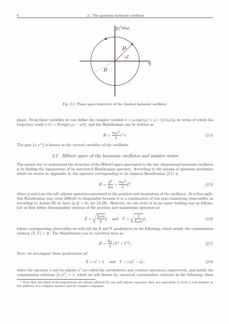
a2 + v2/ω2 as shown in Figure 2.1, returning to its initial point at timestk = 2πk/ω, with k ∈ N. This circular trajectory could have been derived without even solving the equations ofmotion, as the conservation of the Hamiltonian H (t) = H (0) leads directly to q2 + p2/m2ω2 = R2, which is exactlythe circumference of Figure 2.1. This is a simple example of the power of the Hamiltonian formalism.

There is another useful description of the harmonic oscillator, the so called amplitude–phase or complex represen-tation. The amplitude and phase refer to the polar coordinates in phase space, say µ =

√

q2 + p2/m2ω2 and ϕ =arctan (p/mωq), as shown in Figure 2.1. In terms of these variables, the trajectory reads simply (µ, ϕ) = (R,ϕ0 − ωt),with ϕ0 = arctan (v/ωa), so that the evolution is completely described by a linear time variation of the oscillator’s

8 2. The quantum harmonic oscillator

Fig. 2.1: Phase space trajectory of the classical harmonic oscillator.

phase. From these variables we can define the complex variable ν = µ exp (iϕ) = q + (i/mω) p, in terms of which thetrajectory reads ν (t) = R exp[i (ϕ0 − ωt)], and the Hamiltonian can be written as

H =mω2

2ν∗ν. (2.4)

The pair ν, ν∗ is known as the normal variables of the oscillator.

2.2 Hilbert space of the harmonic oscillator and number states

The easiest way to understand the structure of the Hilbert space associated to the one–dimensional harmonic oscillatoris by finding the eigensystem of its associated Hamiltonian operator. According to the axioms of quantum mechanicswhich we review in Appendix A, the operator corresponding to its classical Hamiltonian (2.1) is

H =p2

2m+mω2

2q2, (2.5)

where q and p are the self–adjoint operators associated to the position and momentum of the oscillator. At a first sight,this Hamiltonian may seem difficult to diagonalize because it is a combination of two non-commuting observables, asaccording to Axiom III we have [q, p] = i~, see (A.28). However, we can write it in an easier–looking way as follows.Let us first define dimensionless versions of the position and momentum operators as

X =

√

2ωm

~q and Y =

√

2

~ωmp, (2.6)

whose corresponding observables we will call the X and Y quadratures in the following, which satisfy the commutationrelation [X, Y ] = 2i. The Hamiltonian can be rewritten then as

H =~ω

4(X2 + Y 2). (2.7)

Next, we decompose these quadratures as1

X = a† + a and Y = i(

a† − a)

, (2.8)

where the operator a and its adjoint a† are called the annihilation and creation operators, respectively, and satisfy thecommutation relations

[

a, a†]

= 1, which we will denote by canonical commutation relations in the following; these

1 Note that this kind of decompositions are always allowed for any self–adjoint operator; they are equivalent to write a real number asthe addition of a complex number and its complex conjugate.

2.2. Hilbert space of the harmonic oscillator and number states 9

operators can be seen as the quantum counterparts of the normal variables of the classical oscillator. In terms of theseoperators the Hamiltonian takes the form2

H = ~ω

(

a†a+1

2

)

, (2.11)

and hence the problem is simplified to finding the eigensystem of the self–adjoint operator n = a†a, which we will callthe number operator.

Let us call n to a generic real number contained in the spectrum of n, whose corresponding eigenvector we denoteby |n〉, so that, n|n〉 = n|n〉. We normalize the vectors to one by definition, that is, 〈n|n〉 = 1 ∀n. The eigensystem ofn is readily found from the following two properties:

• n is a positive operator, as for any vector |ψ〉 it is satisfied 〈ψ|n|ψ〉 = (a|ψ〉, a|ψ〉) ≥ 0. When applied to itseigenvectors, this property forbids the existence of negative eigenvalues, that is n ≥ 0.

• Using the commutation relation3 [n, a] = −a, it is trivial to show that the vector a|n〉 is also an eigenvector ofn with eigenvalue n− 1. Similarly, from the commutation relation [n, a†] = a† it is found that the vector a†|n〉is an eigenvector of n with eigenvalue n+ 1.

These two properties imply that the spectrum of n is the set of natural numbers n ∈ 0, 1, 2, ... ≡ N, and thatthe eigenvector |0〉 corresponding to n = 0 must satisfy a|0〉 = 0; otherwise it would be possible to find negativeeigenvalues, hence contradicting the positivity of n. Thus, the set of eigenvectors |n〉n∈N is an infinite, countableset. Moreover, using the property a|0〉 = 0 and the commutation relations, it is easy to prove that the eigenvectorscorresponding to different eigenvalues are orthogonal, that is, 〈n|m〉 = δnm. Finally, according to the axioms ofquantum mechanics only the vectors normalized to one are physically relevant. Hence, we conclude that the spacegenerated by the eigenvectors of n is isomorphic to l2 (∞), and hence it is an infinite–dimensional Hilbert space (seeSection A.2.3).

Summarizing, we have been able to prove that the Hilbert space associated to the one–dimensional harmonicoscillator is infinite–dimensional. In the process, we have explicitly built an orthonormal basis of this space by usingthe eigenvectors |n〉n∈N of the number operator n, with the annihilation and creation operators a, a† allowing usto move through this set as

a|n〉 =√n|n− 1〉 and a†|n〉 =

√n+ 1|n+ 1〉, (2.12)

the factors in the square roots being easily found from normalization requirements.Let us now explain some physical consequences of this. The vectors |n〉n∈N are eigenvectors of the energy (the

Hamiltonian) with eigenvalues En = ~ω(n + 1/2)n∈N, and hence quantum theory predicts that the energy of theoscillator is quantized: Only a discrete set of energies separated by ~ω can be measured in an experiment. The numberof quanta or excitations is given by n, and that’s why n is called the “number” operator, it ‘counts’ the number ofexcitations. Similarly, the creation and annihilation operators receive their names because they add and subtractexcitations. As these vectors have a well defined number of excitations, ∆n = 0, we will call them number states.Consequently, |0〉 will be called the vacuum state of the oscillator, as it has no quanta.

On the other hand, while in classical mechanics the harmonic oscillator can have zero energy —what happens whenit is in its equilibrium state—, quantum mechanics predicts that the minimum energy that the oscillator can have isE0 = ~ω/2 > 0. One way to understand where this zero–point energy comes from is by minimizing the expectationvalue of the Hamiltonian, which can be written as

〈H〉 = ~ω

4(∆X2 +∆Y 2 + 〈X〉2 + 〈Y 〉2), (2.13)

subject to the constraint ∆X∆Y ≥ 1 imposed by the uncertainty principle. It is easy to argue that the minimum valueof 〈H〉 is obtained for the state satisfying ∆X = ∆Y = 1 and 〈X〉 = 〈Y 〉 = 0, which corresponds, not surprisingly,

2 Note that this Hamiltonian could have been obtained by following another quantization procedure based on the normal variables ofthe oscillator. In particular, we could simetrize the classic Hamiltonian (2.4) respect to the normal variables, writing it then as

H =mω2

4(ν∗ν + νν∗) , (2.9)

to then make the classical–to–quantum correspondences

ν →√

2~/mωa and ν∗ →√

2~/mωa†, (2.10)

replacing the Axiom III introduced in Section A.3.2 by [a, a†] = 1, [a, a] = [a†, a†] = 0. This quantization procedure offers an alternativeto the procedure based on the generalized coordinates and momenta of a mechanical system.

3 This is straightforward to find by using the property [AB, C] = A[B, C] + [A, C]B, valid for any three operators A, B, and C.

10 2. The quantum harmonic oscillator

to the vacuum state |0〉. Hence, the energy present in the ground state of the oscillator comes from the fact that theuncertainty principle does not allow its position and momentum to be exactly zero, they have some fluctuations evenin the vacuum state, and this vacuum fluctuations contribute to the energy of the oscillator.

2.3 Coherent states

2.3.1 Connection to classical mechanics

Based on the previous sections, we see that the classical and quantum formalisms seem completely different in essence:While classically the oscillator can have any positive value of the energy and has a definite trajectory in phase space,quantum mechanics allows only for discrete values of the energy and introduces position and momentum uncertaintieswhich prevent the existence of well defined trajectories. In this section we show that, despite their differences, bothdescriptions are compatible in some limit.

Let us first note that, instead of its position and momentum, from now on we take the X and Y quadratures ofthe oscillator as the observables defining the phase space. Using these variables, the classical phase space trajectoryof the oscillator reads (X,Y ) = (X0 cosωt+ Y0 sinωt, Y0 cosωt−X0 sinωt), which defines a circumference of radiusR =

√

X20 + Y 2

0 , being X0 = X (0) and Y0 = Y (0).Quantum mechanics is all about predicting the statistics of experiments, see Section A.3.2. Hence, a way of

connecting it to classical mechanics is by finding the quantum state which predicts that the statistics obtained in theexperiment will coincide with what is classically expected. The following two points explain the properties that sucha state should have in the case of the harmonic oscillator:

• Classically, the energy is a continuous observable. On the hand, the ratio between the energies of two consecutivenumber states is En+1/En = (n+ 3/2)/(n + 1/2); hence, as the number of excitations increases, the discretecharacter of the energy becomes barely perceptive, that is, En+1/En ∼ 1 if n≫ 1. Thus, the state should havea large number of excitations, that is, 〈n〉 ≫ 1.

• The expectation value of the quadratures must describe the classical circular trajectory, while the uncer-tainties of both quadratures should be well below the radius of the circumference defined by it, that is,(〈X (t)〉, 〈Y (t)〉) = (X0 cosωt+ Y0 sinωt, Y0 cosωt−X0 sinωt) with ∆X,∆Y ≪ R. Hence, at all effects theexperimental outcomes predicted by quantum theory for the quadratures will coincide with those expected fromclassical mechanics. Note that the condition for the uncertainties requiresR≫ 1, as we know that ∆X = ∆Y = 1is the minimum simultaneous value that the variances can take.

Then, if states satisfying this properties exist, we see that it is indeed possible to reconcile quantum theory withclassical mechanics at least on what concerns to physical observations.

Our starting point for obtaining these states are the Heisenberg evolution equations for the quadrature operatorsX and Y , which read

d

dtX =

1

i~[X, H] = ωY , (2.14a)

d

dtY =

1

i~[Y , H ] = −ωX, (2.14b)

from which we obtain

X (t) = X (0) cosωt+ Y (0) sinωt, (2.15a)

Y (t) = Y (0) cosωt− X (0) sinωt. (2.15b)

Hence, the expectation values of the quadratures describe the classical trajectories by construction, so that in order toreproduce a classical trajectory with initial quadratures (X0, Y0), the state must satisfy 〈X (0)〉 = X0 and 〈Y (0)〉 = Y0.Writing now the quadratures in terms of the annihilation and creation operators (2.8) these last relations can berecasted as 〈a〉 = (X0 + iY0) /2; being (X0, Y0) arbitrary, this condition shows that the states we are looking for arethe eigenvectors of the annihilation operator, that is, the states |α〉 satisfying a|α〉 = α|α〉 with α = (X0 + iY0) /2 ∈ C.We will call coherent states to the eigenvectors of the annihilation operator.

It is straightforward to show that, in addition, coherent states have 〈n〉 = |α|2, R = 2|α| and ∆X = ∆Y = 1, sothat in the limit |α| ≫ 1 they satisfy all the requisites that we needed to make the connection with classical mechanics.Note that these properties hold at any time.

In the following we show that the eigenvectors of the annihilation operator exist by finding an explicit representationof them in the Hilbert space of the oscillator, and discuss some of their properties.

2.3. Coherent states 11

2.3.2 Properties of the coherent states

It is simple to find an explicit representation of the coherent states in terms of the basis of number states, that is, tofind the coefficients cn of the expansion |α〉 = ∑∞

n=0 cn|n〉. Introducing this expansion in the eigenvector equation4

a|α〉 = α|α〉, we find the simple recurrence

cn =α√ncn−1 =⇒ cn =

αn√n!c0. (2.16)

On the other hand, the determination of c0 comes from the normalization condition

〈α|α〉 = 1 = |c0|2∞∑

n=0

|α|2/n! =⇒ c0 = exp

(

−|α|2

2

)

, (2.17)

where we have chosen c0 to be a positive real as the global phase of the state cannot play any physical role5. Hence,the coherent states are finally written as

|α〉 =∞∑

n=0

e−|α|2/2 α

n

√n!|n〉. (2.18)

Note that for α = 0, coherent states are equivalent to the vacuum state, that is, |α = 0〉 = |n = 0〉. For any other valueof α coherent states do not have a well defined number of excitations; instead, the number of quanta is distributedaccording to a Poissonian probability distribution

Pn (α) = |〈n|α〉|2 = e−|α|2 |α|2nn!

. (2.19)

Let us now define the displacement operator

D (α) = exp(

αa† − α∗a)

; (2.20)

the general formula exp(A + B) = exp(−[A, B]/2) exp(A) exp(B), valid for operators A and B which commute withtheir commutator, allows us to write it also as

D(n) (α) = exp(

−|α|2/2)

exp(

αa†)

exp (−α∗a) , (2.21)

orD(a) (α) = exp

(

|α|2/2)

exp (−α∗a) exp(

αa†)

, (2.22)

which we will refer to as its normal and antinormal forms, respectively6. Coherent states can then be obtained bydisplacing vacuum

|α〉 = D (α) |0〉, (2.23)

what is trivially proved using the normal form of the displacement operator. This is interesting because the displace-ment operator is unitary by construction, that is, D† (α) D (α) = D (α) D† (α) = I, and hence the coherent state |α〉can be created from a vacuum–state oscillator by making it evolve with a Hamiltonian HD = i~(αa† −α∗a)/T duringa time T . This is in contrast to the number states, which cannot be generated by unitary evolution of the oscillatorin any way.

Note that when a displacement is applied to the annihilation and creation operators, we get7

D† (α) aD (α) = a+ α and D† (α) a†D (α) = a† + α∗, (2.25)

4 On a second thought, the existence of states satisfying this equation is kind of amazing: Consider for example a coherent state with|α|2 ≪ 1, so that we are sure that the mean number of excitations is really below one; this equation states that we can still annihilate asmany excitations as we want without altering the state!

5 This is evident since we have formulated quantum mechanics in terms of the density operator, which for all pure states eiφ|ψ〉 readsρ = |ψ〉〈ψ| irrespective of φ (see Section A.3.2).

6 With full generality, given an operator A(a, a†

), we denote by A(n)

(a, a†

)and A(a)

(a, a†

)its normal and antinormal forms. A(n)

and A(a) are obtained by writing A(a, a†

)with all the creation operators to the left or to the right, respectively, with the help of the

commutation relations. Hence, for example, the operator A = aa†a has A(n) = a†a2 + a and A(a) = a2a† − a as normal and antinormalforms.

7 This is trivially proved by using the Baker–Campbell–Haussdorf lemma

eBAe−B =∞∑

n=0

1

n![B, [B, ...[B,︸ ︷︷ ︸

n

A]...]]︸︷︷︸

n

, (2.24)

valid for two general operators A and B.

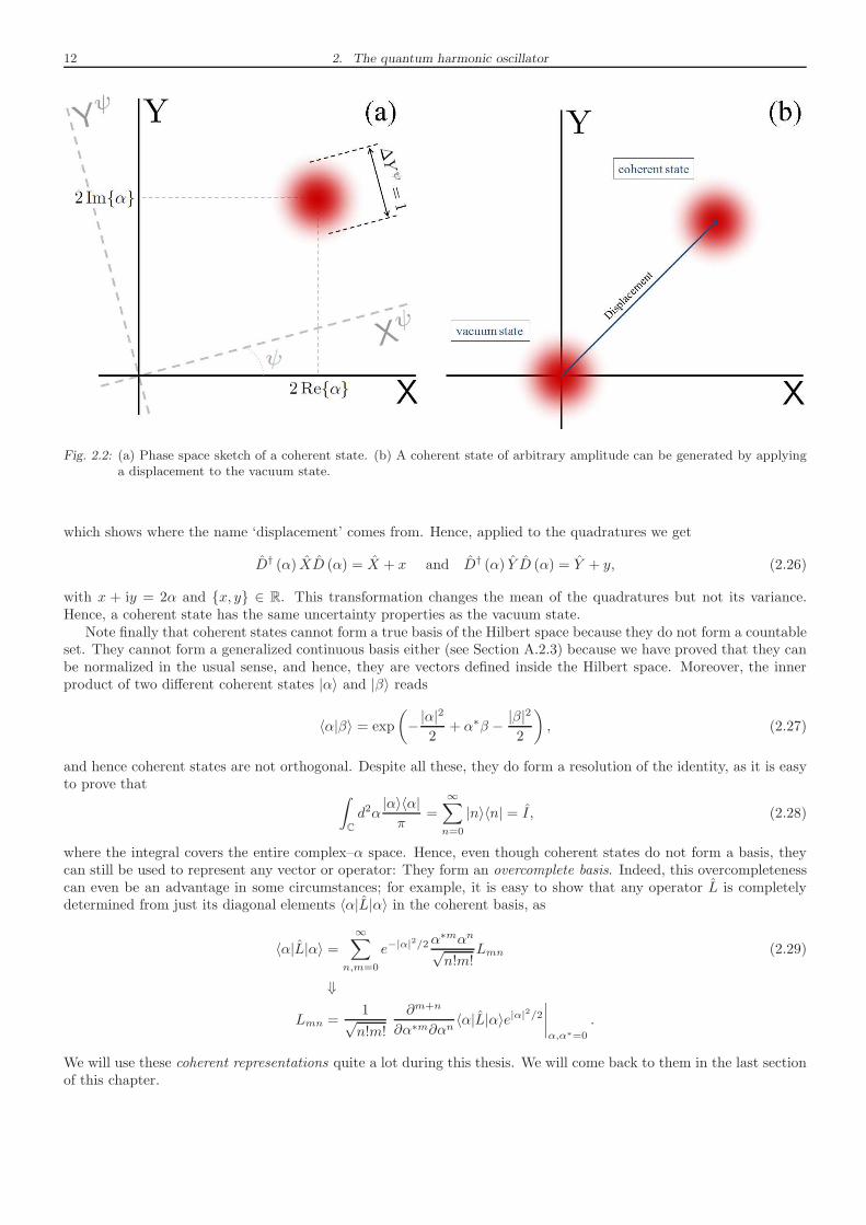
12 2. The quantum harmonic oscillator

Fig. 2.2: (a) Phase space sketch of a coherent state. (b) A coherent state of arbitrary amplitude can be generated by applyinga displacement to the vacuum state.

which shows where the name ‘displacement’ comes from. Hence, applied to the quadratures we get

D† (α) XD (α) = X + x and D† (α) Y D (α) = Y + y, (2.26)

with x + iy = 2α and x, y ∈ R. This transformation changes the mean of the quadratures but not its variance.Hence, a coherent state has the same uncertainty properties as the vacuum state.

Note finally that coherent states cannot form a true basis of the Hilbert space because they do not form a countableset. They cannot form a generalized continuous basis either (see Section A.2.3) because we have proved that they canbe normalized in the usual sense, and hence, they are vectors defined inside the Hilbert space. Moreover, the innerproduct of two different coherent states |α〉 and |β〉 reads

〈α|β〉 = exp

(

−|α|2

2+ α∗β − |β|

2

2

)

, (2.27)

and hence coherent states are not orthogonal. Despite all these, they do form a resolution of the identity, as it is easyto prove that

∫

C

d2α|α〉〈α|π

=

∞∑

n=0

|n〉〈n| = I , (2.28)

where the integral covers the entire complex–α space. Hence, even though coherent states do not form a basis, theycan still be used to represent any vector or operator: They form an overcomplete basis. Indeed, this overcompletenesscan even be an advantage in some circumstances; for example, it is easy to show that any operator L is completelydetermined from just its diagonal elements 〈α|L|α〉 in the coherent basis, as

〈α|L|α〉 =∞∑

n,m=0

e−|α|2/2α

∗mαn√n!m!

Lmn (2.29)

⇓

Lmn =1√n!m!

∂m+n

∂α∗m∂αn〈α|L|α〉e|α|2/2

∣

∣

∣

∣

α,α∗=0

.

We will use these coherent representations quite a lot during this thesis. We will come back to them in the last sectionof this chapter.

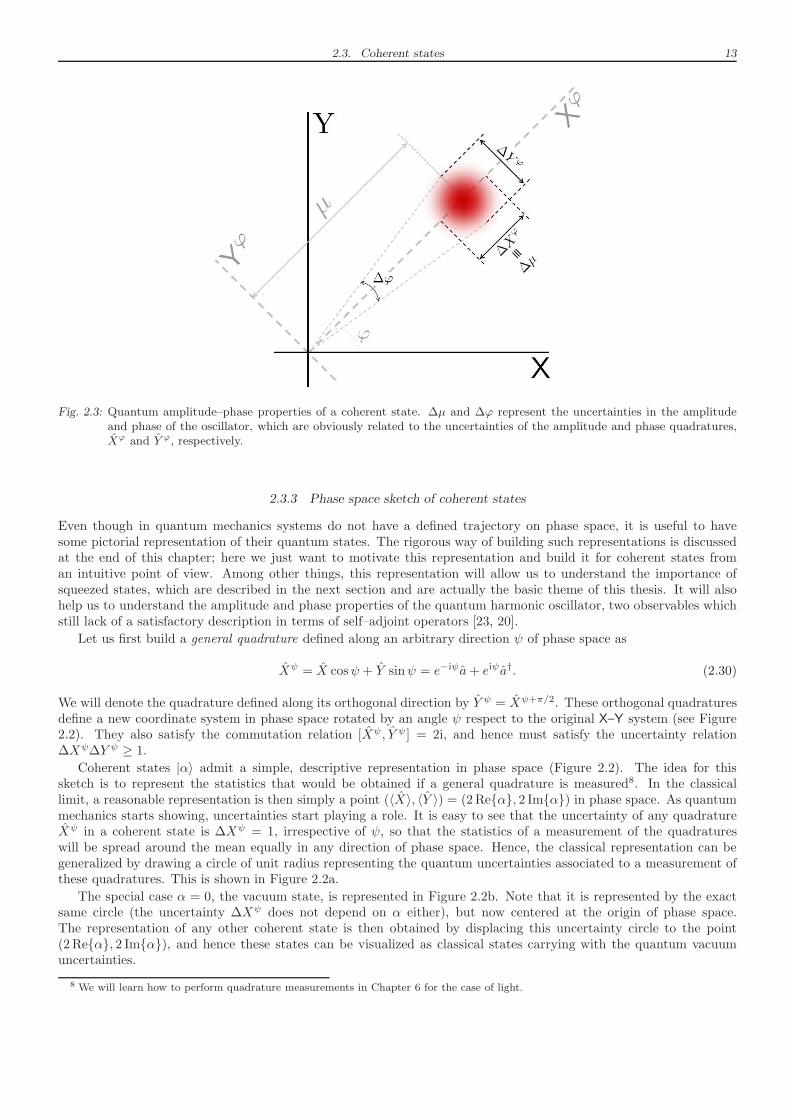
2.3. Coherent states 13

Fig. 2.3: Quantum amplitude–phase properties of a coherent state. ∆µ and ∆ϕ represent the uncertainties in the amplitudeand phase of the oscillator, which are obviously related to the uncertainties of the amplitude and phase quadratures,Xϕ and Y ϕ, respectively.

2.3.3 Phase space sketch of coherent states

Even though in quantum mechanics systems do not have a defined trajectory on phase space, it is useful to havesome pictorial representation of their quantum states. The rigorous way of building such representations is discussedat the end of this chapter; here we just want to motivate this representation and build it for coherent states froman intuitive point of view. Among other things, this representation will allow us to understand the importance ofsqueezed states, which are described in the next section and are actually the basic theme of this thesis. It will alsohelp us to understand the amplitude and phase properties of the quantum harmonic oscillator, two observables whichstill lack of a satisfactory description in terms of self–adjoint operators [23, 20].

Let us first build a general quadrature defined along an arbitrary direction ψ of phase space as

Xψ = X cosψ + Y sinψ = e−iψa+ eiψa†. (2.30)

We will denote the quadrature defined along its orthogonal direction by Y ψ = Xψ+π/2. These orthogonal quadraturesdefine a new coordinate system in phase space rotated by an angle ψ respect to the original X–Y system (see Figure2.2). They also satisfy the commutation relation [Xψ, Y ψ] = 2i, and hence must satisfy the uncertainty relation∆Xψ∆Y ψ ≥ 1.

Coherent states |α〉 admit a simple, descriptive representation in phase space (Figure 2.2). The idea for thissketch is to represent the statistics that would be obtained if a general quadrature is measured8. In the classicallimit, a reasonable representation is then simply a point (〈X〉, 〈Y 〉) = (2Reα, 2 Imα) in phase space. As quantummechanics starts showing, uncertainties start playing a role. It is easy to see that the uncertainty of any quadratureXψ in a coherent state is ∆Xψ = 1, irrespective of ψ, so that the statistics of a measurement of the quadratureswill be spread around the mean equally in any direction of phase space. Hence, the classical representation can begeneralized by drawing a circle of unit radius representing the quantum uncertainties associated to a measurement ofthese quadratures. This is shown in Figure 2.2a.

The special case α = 0, the vacuum state, is represented in Figure 2.2b. Note that it is represented by the exactsame circle (the uncertainty ∆Xψ does not depend on α either), but now centered at the origin of phase space.The representation of any other coherent state is then obtained by displacing this uncertainty circle to the point(2Reα, 2 Imα), and hence these states can be visualized as classical states carrying with the quantum vacuumuncertainties.

8 We will learn how to perform quadrature measurements in Chapter 6 for the case of light.

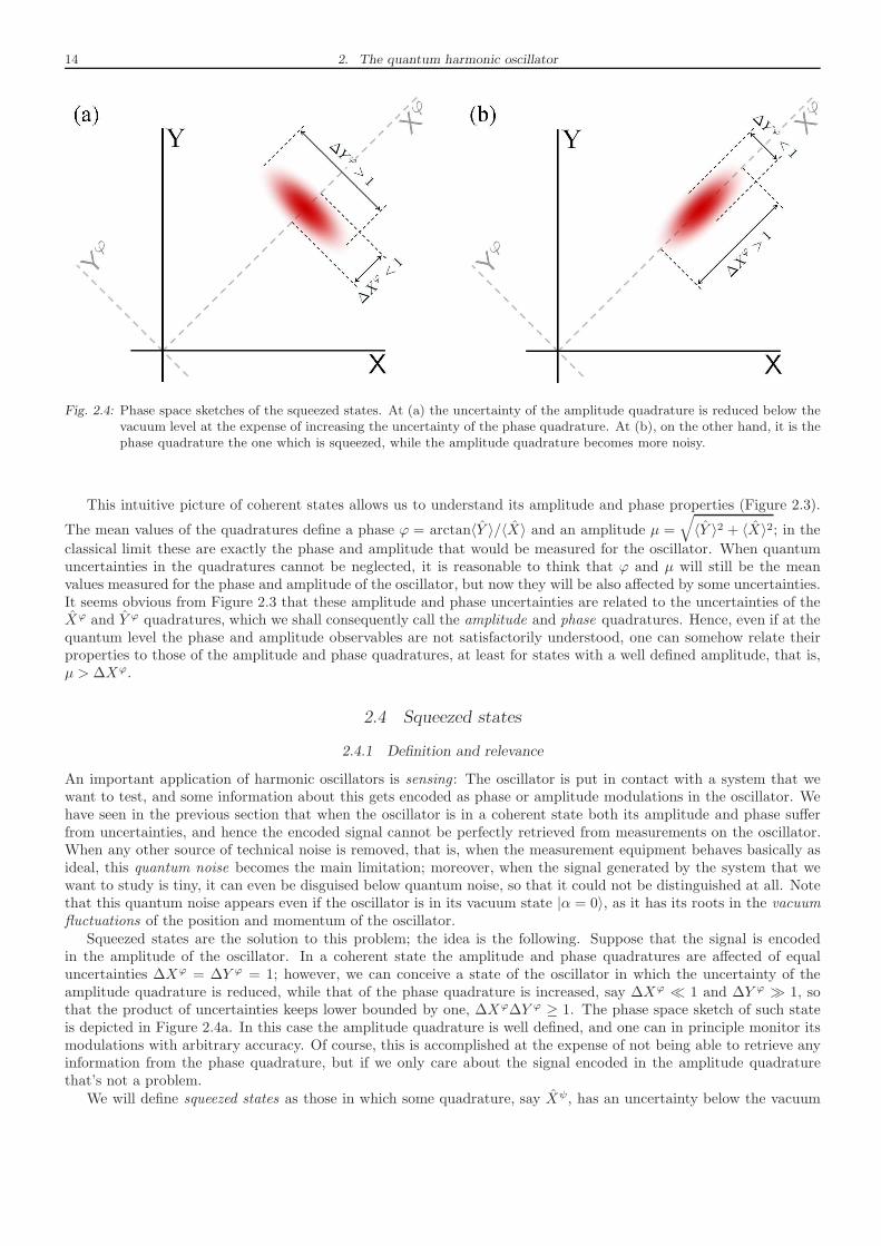
14 2. The quantum harmonic oscillator

Fig. 2.4: Phase space sketches of the squeezed states. At (a) the uncertainty of the amplitude quadrature is reduced below thevacuum level at the expense of increasing the uncertainty of the phase quadrature. At (b), on the other hand, it is thephase quadrature the one which is squeezed, while the amplitude quadrature becomes more noisy.

This intuitive picture of coherent states allows us to understand its amplitude and phase properties (Figure 2.3).

The mean values of the quadratures define a phase ϕ = arctan〈Y 〉/〈X〉 and an amplitude µ =

√

〈Y 〉2 + 〈X〉2; in the

classical limit these are exactly the phase and amplitude that would be measured for the oscillator. When quantumuncertainties in the quadratures cannot be neglected, it is reasonable to think that ϕ and µ will still be the meanvalues measured for the phase and amplitude of the oscillator, but now they will be also affected by some uncertainties.It seems obvious from Figure 2.3 that these amplitude and phase uncertainties are related to the uncertainties of theXϕ and Y ϕ quadratures, which we shall consequently call the amplitude and phase quadratures. Hence, even if at thequantum level the phase and amplitude observables are not satisfactorily understood, one can somehow relate theirproperties to those of the amplitude and phase quadratures, at least for states with a well defined amplitude, that is,µ > ∆Xϕ.

2.4 Squeezed states

2.4.1 Definition and relevance

An important application of harmonic oscillators is sensing: The oscillator is put in contact with a system that wewant to test, and some information about this gets encoded as phase or amplitude modulations in the oscillator. Wehave seen in the previous section that when the oscillator is in a coherent state both its amplitude and phase sufferfrom uncertainties, and hence the encoded signal cannot be perfectly retrieved from measurements on the oscillator.When any other source of technical noise is removed, that is, when the measurement equipment behaves basically asideal, this quantum noise becomes the main limitation; moreover, when the signal generated by the system that wewant to study is tiny, it can even be disguised below quantum noise, so that it could not be distinguished at all. Notethat this quantum noise appears even if the oscillator is in its vacuum state |α = 0〉, as it has its roots in the vacuumfluctuations of the position and momentum of the oscillator.

Squeezed states are the solution to this problem; the idea is the following. Suppose that the signal is encodedin the amplitude of the oscillator. In a coherent state the amplitude and phase quadratures are affected of equaluncertainties ∆Xϕ = ∆Y ϕ = 1; however, we can conceive a state of the oscillator in which the uncertainty of theamplitude quadrature is reduced, while that of the phase quadrature is increased, say ∆Xϕ ≪ 1 and ∆Y ϕ ≫ 1, sothat the product of uncertainties keeps lower bounded by one, ∆Xϕ∆Y ϕ ≥ 1. The phase space sketch of such stateis depicted in Figure 2.4a. In this case the amplitude quadrature is well defined, and one can in principle monitor itsmodulations with arbitrary accuracy. Of course, this is accomplished at the expense of not being able to retrieve anyinformation from the phase quadrature, but if we only care about the signal encoded in the amplitude quadraturethat’s not a problem.

We will define squeezed states as those in which some quadrature, say Xψ, has an uncertainty below the vacuum

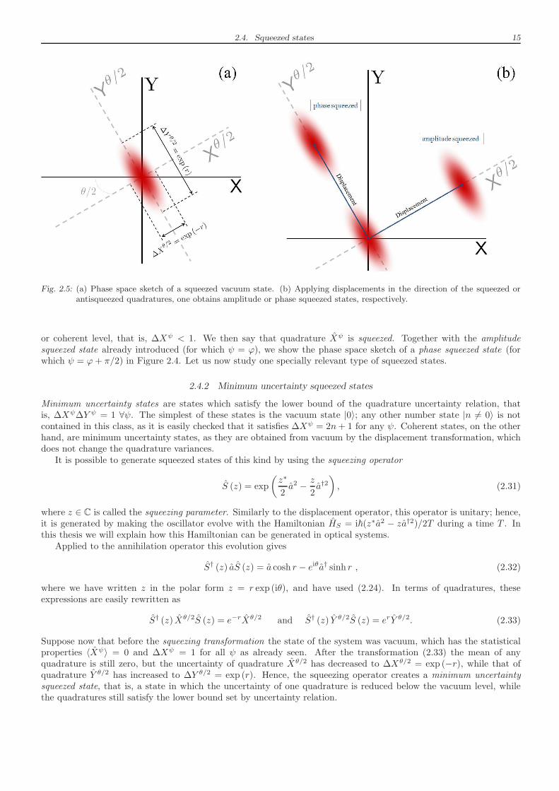
2.4. Squeezed states 15

Fig. 2.5: (a) Phase space sketch of a squeezed vacuum state. (b) Applying displacements in the direction of the squeezed orantisqueezed quadratures, one obtains amplitude or phase squeezed states, respectively.

or coherent level, that is, ∆Xψ < 1. We then say that quadrature Xψ is squeezed. Together with the amplitudesqueezed state already introduced (for which ψ = ϕ), we show the phase space sketch of a phase squeezed state (forwhich ψ = ϕ+ π/2) in Figure 2.4. Let us now study one specially relevant type of squeezed states.

2.4.2 Minimum uncertainty squeezed states

Minimum uncertainty states are states which satisfy the lower bound of the quadrature uncertainty relation, thatis, ∆Xψ∆Y ψ = 1 ∀ψ. The simplest of these states is the vacuum state |0〉; any other number state |n 6= 0〉 is notcontained in this class, as it is easily checked that it satisfies ∆Xψ = 2n+ 1 for any ψ. Coherent states, on the otherhand, are minimum uncertainty states, as they are obtained from vacuum by the displacement transformation, whichdoes not change the quadrature variances.

It is possible to generate squeezed states of this kind by using the squeezing operator

S (z) = exp

(

z∗

2a2 − z

2a†2)

, (2.31)

where z ∈ C is called the squeezing parameter. Similarly to the displacement operator, this operator is unitary; hence,it is generated by making the oscillator evolve with the Hamiltonian HS = i~(z∗a2 − za†2)/2T during a time T . Inthis thesis we will explain how this Hamiltonian can be generated in optical systems.

Applied to the annihilation operator this evolution gives

S† (z) aS (z) = a cosh r − eiθa† sinh r , (2.32)

where we have written z in the polar form z = r exp (iθ), and have used (2.24). In terms of quadratures, theseexpressions are easily rewritten as

S† (z) Xθ/2S (z) = e−rXθ/2 and S† (z) Y θ/2S (z) = erY θ/2. (2.33)

Suppose now that before the squeezing transformation the state of the system was vacuum, which has the statisticalproperties 〈Xψ〉 = 0 and ∆Xψ = 1 for all ψ as already seen. After the transformation (2.33) the mean of anyquadrature is still zero, but the uncertainty of quadrature Xθ/2 has decreased to ∆Xθ/2 = exp (−r), while that ofquadrature Y θ/2 has increased to ∆Y θ/2 = exp (r). Hence, the squeezing operator creates a minimum uncertaintysqueezed state, that is, a state in which the uncertainty of one quadrature is reduced below the vacuum level, whilethe quadratures still satisfy the lower bound set by uncertainty relation.

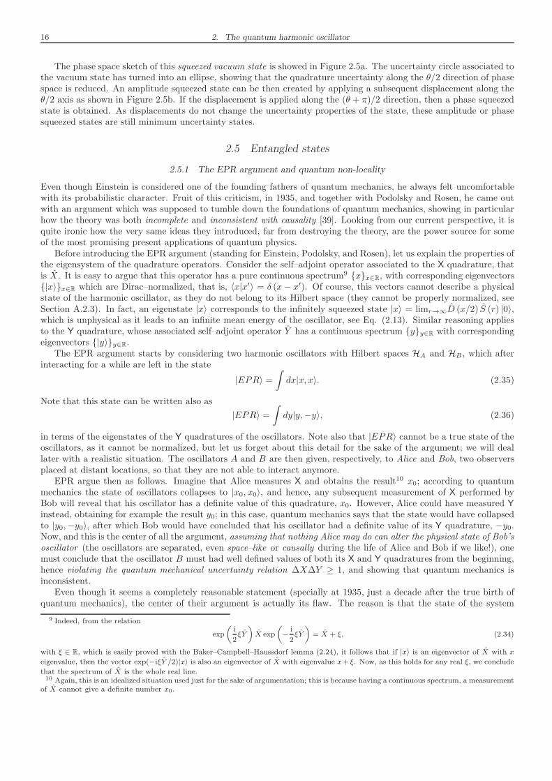
16 2. The quantum harmonic oscillator

The phase space sketch of this squeezed vacuum state is showed in Figure 2.5a. The uncertainty circle associated tothe vacuum state has turned into an ellipse, showing that the quadrature uncertainty along the θ/2 direction of phasespace is reduced. An amplitude squeezed state can be then created by applying a subsequent displacement along theθ/2 axis as shown in Figure 2.5b. If the displacement is applied along the (θ + π)/2 direction, then a phase squeezedstate is obtained. As displacements do not change the uncertainty properties of the state, these amplitude or phasesqueezed states are still minimum uncertainty states.

2.5 Entangled states

2.5.1 The EPR argument and quantum non-locality

Even though Einstein is considered one of the founding fathers of quantum mechanics, he always felt uncomfortablewith its probabilistic character. Fruit of this criticism, in 1935, and together with Podolsky and Rosen, he came outwith an argument which was supposed to tumble down the foundations of quantum mechanics, showing in particularhow the theory was both incomplete and inconsistent with causality [39]. Looking from our current perspective, it isquite ironic how the very same ideas they introduced, far from destroying the theory, are the power source for someof the most promising present applications of quantum physics.

Before introducing the EPR argument (standing for Einstein, Podolsky, and Rosen), let us explain the properties ofthe eigensystem of the quadrature operators. Consider the self–adjoint operator associated to the X quadrature, thatis X. It is easy to argue that this operator has a pure continuous spectrum9 xx∈R, with corresponding eigenvectors|x〉x∈R which are Dirac–normalized, that is, 〈x|x′〉 = δ (x− x′). Of course, this vectors cannot describe a physicalstate of the harmonic oscillator, as they do not belong to its Hilbert space (they cannot be properly normalized, seeSection A.2.3). In fact, an eigenstate |x〉 corresponds to the infinitely squeezed state |x〉 = limr→∞D (x/2) S (r) |0〉,which is unphysical as it leads to an infinite mean energy of the oscillator, see Eq. (2.13). Similar reasoning appliesto the Y quadrature, whose associated self–adjoint operator Y has a continuous spectrum yy∈R with correspondingeigenvectors |y〉y∈R.

The EPR argument starts by considering two harmonic oscillators with Hilbert spaces HA and HB, which afterinteracting for a while are left in the state

|EPR〉 =∫

dx|x, x〉. (2.35)

Note that this state can be written also as

|EPR〉 =∫

dy|y,−y〉, (2.36)

in terms of the eigenstates of the Y quadratures of the oscillators. Note also that |EPR〉 cannot be a true state of theoscillators, as it cannot be normalized, but let us forget about this detail for the sake of the argument; we will deallater with a realistic situation. The oscillators A and B are then given, respectively, to Alice and Bob, two observersplaced at distant locations, so that they are not able to interact anymore.

EPR argue then as follows. Imagine that Alice measures X and obtains the result10 x0; according to quantummechanics the state of oscillators collapses to |x0, x0〉, and hence, any subsequent measurement of X performed byBob will reveal that his oscillator has a definite value of this quadrature, x0. However, Alice could have measured Y

instead, obtaining for example the result y0; in this case, quantum mechanics says that the state would have collapsedto |y0,−y0〉, after which Bob would have concluded that his oscillator had a definite value of its Y quadrature, −y0.Now, and this is the center of all the argument, assuming that nothing Alice may do can alter the physical state of Bob’soscillator (the oscillators are separated, even space–like or causally during the life of Alice and Bob if we like!), onemust conclude that the oscillator B must had well defined values of both its X and Y quadratures from the beginning,hence violating the quantum mechanical uncertainty relation ∆X∆Y ≥ 1, and showing that quantum mechanics isinconsistent.

Even though it seems a completely reasonable statement (specially at 1935, just a decade after the true birth ofquantum mechanics), the center of their argument is actually its flaw. The reason is that the state of the system

9 Indeed, from the relation

exp

(i

2ξY

)

X exp

(

−i

2ξY

)

= X + ξ, (2.34)

with ξ ∈ R, which is easily proved with the Baker–Campbell–Haussdorf lemma (2.24), it follows that if |x〉 is an eigenvector of X with x

eigenvalue, then the vector exp(−iξY /2)|x〉 is also an eigenvector of X with eigenvalue x+ ξ. Now, as this holds for any real ξ, we conclude

that the spectrum of X is the whole real line.10 Again, this is an idealized situation used just for the sake of argumentation; this is because having a continuous spectrum, a measurement

of X cannot give a definite number x0.

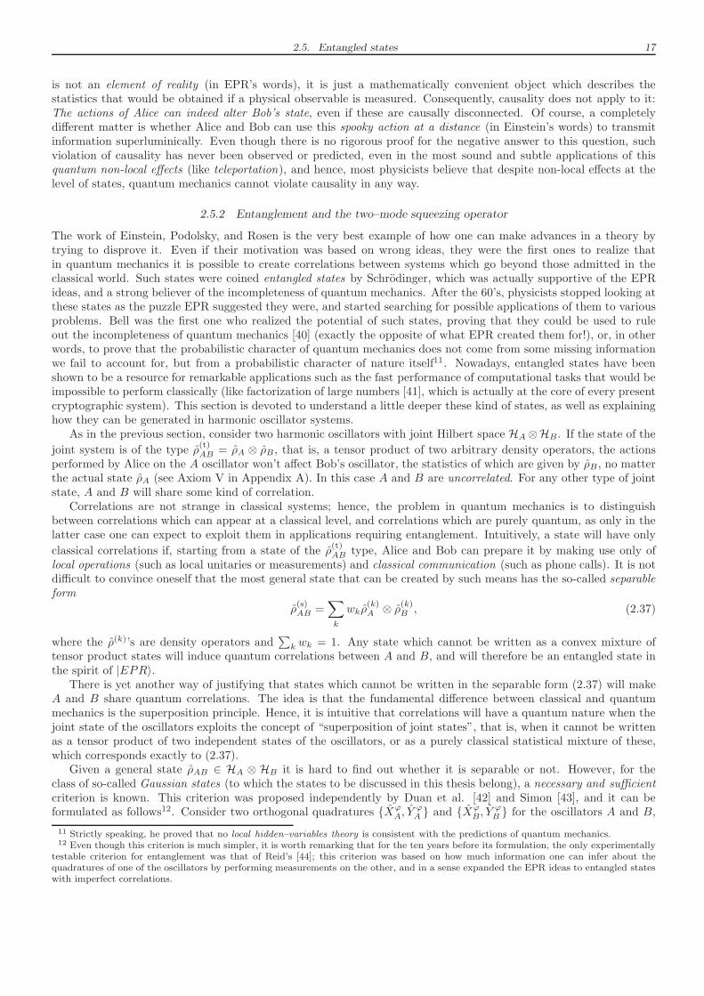
2.5. Entangled states 17

is not an element of reality (in EPR’s words), it is just a mathematically convenient object which describes thestatistics that would be obtained if a physical observable is measured. Consequently, causality does not apply to it:The actions of Alice can indeed alter Bob’s state, even if these are causally disconnected. Of course, a completelydifferent matter is whether Alice and Bob can use this spooky action at a distance (in Einstein’s words) to transmitinformation superluminically. Even though there is no rigorous proof for the negative answer to this question, suchviolation of causality has never been observed or predicted, even in the most sound and subtle applications of thisquantum non-local effects (like teleportation), and hence, most physicists believe that despite non-local effects at thelevel of states, quantum mechanics cannot violate causality in any way.

2.5.2 Entanglement and the two–mode squeezing operator

The work of Einstein, Podolsky, and Rosen is the very best example of how one can make advances in a theory bytrying to disprove it. Even if their motivation was based on wrong ideas, they were the first ones to realize thatin quantum mechanics it is possible to create correlations between systems which go beyond those admitted in theclassical world. Such states were coined entangled states by Schrodinger, which was actually supportive of the EPRideas, and a strong believer of the incompleteness of quantum mechanics. After the 60’s, physicists stopped looking atthese states as the puzzle EPR suggested they were, and started searching for possible applications of them to variousproblems. Bell was the first one who realized the potential of such states, proving that they could be used to ruleout the incompleteness of quantum mechanics [40] (exactly the opposite of what EPR created them for!), or, in otherwords, to prove that the probabilistic character of quantum mechanics does not come from some missing informationwe fail to account for, but from a probabilistic character of nature itself11. Nowadays, entangled states have beenshown to be a resource for remarkable applications such as the fast performance of computational tasks that would beimpossible to perform classically (like factorization of large numbers [41], which is actually at the core of every presentcryptographic system). This section is devoted to understand a little deeper these kind of states, as well as explaininghow they can be generated in harmonic oscillator systems.

As in the previous section, consider two harmonic oscillators with joint Hilbert space HA⊗HB. If the state of the

joint system is of the type ρ(t)AB = ρA ⊗ ρB, that is, a tensor product of two arbitrary density operators, the actions

performed by Alice on the A oscillator won’t affect Bob’s oscillator, the statistics of which are given by ρB, no matterthe actual state ρA (see Axiom V in Appendix A). In this case A and B are uncorrelated. For any other type of jointstate, A and B will share some kind of correlation.

Correlations are not strange in classical systems; hence, the problem in quantum mechanics is to distinguishbetween correlations which can appear at a classical level, and correlations which are purely quantum, as only in thelatter case one can expect to exploit them in applications requiring entanglement. Intuitively, a state will have only

classical correlations if, starting from a state of the ρ(t)AB type, Alice and Bob can prepare it by making use only of

local operations (such as local unitaries or measurements) and classical communication (such as phone calls). It is notdifficult to convince oneself that the most general state that can be created by such means has the so-called separableform

ρ(s)AB =

∑

k

wkρ(k)A ⊗ ρ

(k)B , (2.37)

where the ρ(k)’s are density operators and∑

k wk = 1. Any state which cannot be written as a convex mixture oftensor product states will induce quantum correlations between A and B, and will therefore be an entangled state inthe spirit of |EPR〉.

There is yet another way of justifying that states which cannot be written in the separable form (2.37) will makeA and B share quantum correlations. The idea is that the fundamental difference between classical and quantummechanics is the superposition principle. Hence, it is intuitive that correlations will have a quantum nature when thejoint state of the oscillators exploits the concept of “superposition of joint states”, that is, when it cannot be writtenas a tensor product of two independent states of the oscillators, or as a purely classical statistical mixture of these,which corresponds exactly to (2.37).

Given a general state ρAB ∈ HA ⊗ HB it is hard to find out whether it is separable or not. However, for theclass of so-called Gaussian states (to which the states to be discussed in this thesis belong), a necessary and sufficientcriterion is known. This criterion was proposed independently by Duan et al. [42] and Simon [43], and it can beformulated as follows12. Consider two orthogonal quadratures Xϕ

A, YϕA and X

ϕB, Y

ϕB for the oscillators A and B,

11 Strictly speaking, he proved that no local hidden–variables theory is consistent with the predictions of quantum mechanics.12 Even though this criterion is much simpler, it is worth remarking that for the ten years before its formulation, the only experimentally

testable criterion for entanglement was that of Reid’s [44]; this criterion was based on how much information one can infer about thequadratures of one of the oscillators by performing measurements on the other, and in a sense expanded the EPR ideas to entangled stateswith imperfect correlations.

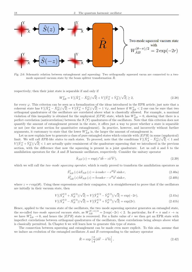
18 2. The quantum harmonic oscillator

Fig. 2.6: Schematic relation between entanglement and squeezing: Two orthogonally squeezed vacua are connected to a two-mode squeezed vacuum state by the beam splitter transformation R.

respectively; then their joint state is separable if and only if

WϕAB = V [(Xϕ

A − XϕB)/√2] + V [(Y ϕA + Y ϕB )/

√2] ≥ 2, (2.38)

for every ϕ. This criterion can be seen as a formalization of the ideas introduced in the EPR article; just note that acoherent state has V [(Xϕ

A − XϕB)/√2] = V [(Y ϕA + Y ϕB )/

√2] = 1 ∀ϕ, and hence if Wϕ

AB < 2 one can be sure that twoorthogonal quadratures of the oscillators are correlated above what is classically allowed. For example, a maximalviolation of this inequality is obtained for the unphysical |EPR〉 state, which has W 0

AB = 0, showing that there is aperfect correlation (anticorrelation) between the X (Y) quadratures of the oscillators. Note that this criterion does notquantify the amount of entanglement present in the state, it offers just a way to prove whether a state is separableor not (see the next section for quantitative entanglement). In practice, however, and incorrectly without furtherarguments, it customary to state that the lower Wϕ

AB is, the larger the amount of entanglement is.Let us now explain how to generate a class of pure entangled states which coincide with |EPR〉 in some (unphysical)

limit. We will call EPR-like states to such states. To proceed, note that the conditions V [(XϕA − X

ϕB)/√2] < 1 and

V [(Y ϕA + Y ϕB )/√2] < 1 are actually quite reminiscent of the quadrature squeezing that we introduced in the previous

section, with the difference that now the squeezing is present in a joint quadrature. Let us call a and b to theannihilation operators for the A and B harmonic oscillators, respectively. Consider the unitary operator

SAB (z) = exp(z∗ab − za†b†), (2.39)

which we will call the two–mode squeezing operator, which is easily proved to transform the annihilation operators as

S†AB (z) aSAB (z) = a cosh r − eiθ b† sinh r, (2.40a)

S†AB (z) bSAB (z) = b cosh r − eiθa† sinh r, (2.40b)

where z = r exp(iθ). Using these expressions and their conjugates, it is straightforward to prove that if the oscillatorsare initially in their vacuum state, then

V [(Xθ/2A + X

θ/2B )/

√2] = V [(Y

θ/2A − Y θ/2B )/

√2] = exp(−2r), (2.41a)

V [(Xθ/2A − Xθ/2

B )/√2] = V [(Y

θ/2A + Y

θ/2B )/

√2] = exp(2r). (2.41b)

Hence, applied to the vacuum state of the oscillators, the two–mode squeezing operator generates an entangled state,

the so-called two–mode squeezed vacuum state, as W(θ−π)/2AB = 2 exp(−2r) < 2. In particular, for θ = π and r → ∞

we have W 0AB → 0, and hence the |EPR〉 state is recovered. For a finite value of r we then get an EPR state with

imperfect correlations between orthogonal quadratures of the oscillators, these correlations being always above whatis classically permitted. In Chapter 6 we will learn how to generate this type of states.

The connection between squeezing and entanglement can be made even more explicit. To this aim, assume thatwe induce an evolution of the entangled oscillators A and B corresponding to the unitary operator

R = exp[π

4(ab† − a†b)

]

, (2.42)

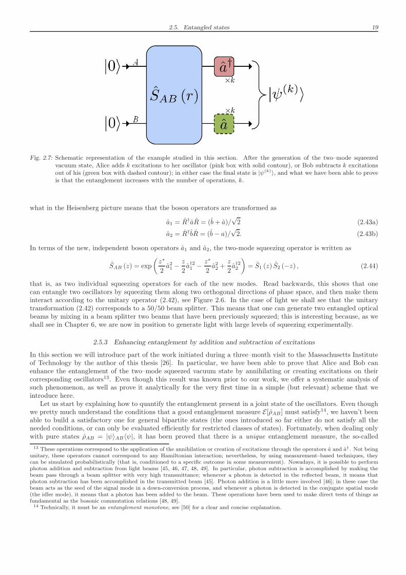
2.5. Entangled states 19

Fig. 2.7: Schematic representation of the example studied in this section. After the generation of the two–mode squeezedvacuum state, Alice adds k excitations to her oscillator (pink box with solid contour), or Bob subtracts k excitationsout of his (green box with dashed contour); in either case the final state is |ψ(k)〉, and what we have been able to proveis that the entanglement increases with the number of operations, k.

what in the Heisenberg picture means that the boson operators are transformed as

a1 = R†aR = (b+ a)/√2 (2.43a)

a2 = R†bR = (b − a)/√2. (2.43b)

In terms of the new, independent boson operators a1 and a2, the two-mode squeezing operator is written as

SAB (z) = exp

(

z∗

2a21 −

z

2a†21 −

z∗

2a22 +

z

2a†22

)

= S1 (z) S2 (−z) , (2.44)

that is, as two individual squeezing operators for each of the new modes. Read backwards, this shows that onecan entangle two oscillators by squeezing them along two orthogonal directions of phase space, and then make theminteract according to the unitary operator (2.42), see Figure 2.6. In the case of light we shall see that the unitarytransformation (2.42) corresponds to a 50/50 beam splitter. This means that one can generate two entangled opticalbeams by mixing in a beam splitter two beams that have been previously squeezed; this is interesting because, as weshall see in Chapter 6, we are now in position to generate light with large levels of squeezing experimentally.

2.5.3 Enhancing entanglement by addition and subtraction of excitations

In this section we will introduce part of the work initiated during a three–month visit to the Massachusetts Instituteof Technology by the author of this thesis [26]. In particular, we have been able to prove that Alice and Bob canenhance the entanglement of the two–mode squeezed vacuum state by annihilating or creating excitations on theircorresponding oscillators13. Even though this result was known prior to our work, we offer a systematic analysis ofsuch phenomenon, as well as prove it analytically for the very first time in a simple (but relevant) scheme that weintroduce here.

Let us start by explaining how to quantify the entanglement present in a joint state of the oscillators. Even thoughwe pretty much understand the conditions that a good entanglement measure E [ρAB] must satisfy14, we haven’t beenable to build a satisfactory one for general bipartite states (the ones introduced so far either do not satisfy all theneeded conditions, or can only be evaluated efficiently for restricted classes of states). Fortunately, when dealing onlywith pure states ρAB = |ψ〉AB〈ψ|, it has been proved that there is a unique entanglement measure, the so-called

13 These operations correspond to the application of the annihilation or creation of excitations through the operators a and a†. Not beingunitary, these operators cannot correspond to any Hamiltonian interaction; nevertheless, by using measurement–based techniques, theycan be simulated probabilistically (that is, conditioned to a specific outcome in some measurement). Nowadays, it is possible to performphoton addition and subtraction from light beams [45, 46, 47, 48, 49]. In particular, photon subtraction is accomplished by making thebeam pass through a beam splitter with very high transmittance; whenever a photon is detected in the reflected beam, it means thatphoton subtraction has been accomplished in the transmitted beam [45]. Photon addition is a little more involved [46]; in these case thebeam acts as the seed of the signal mode in a down-conversion process, and whenever a photon is detected in the conjugate spatial mode(the idler mode), it means that a photon has been added to the beam. These operations have been used to make direct tests of things asfundamental as the bosonic commutation relations [48, 49].14 Technically, it must be an entanglement monotone, see [50] for a clear and concise explanation.

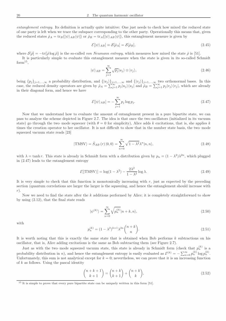
20 2. The quantum harmonic oscillator

entanglement entropy. Its definition is actually quite intuitive: One just needs to check how mixed the reduced stateof one party is left when we trace the subspace corresponding to the other party. Operationally this means that, giventhe reduced states ρA = trB|ψ〉AB〈ψ| or ρB = trA|ψ〉AB〈ψ|, this entanglement measure is given by

E [|ψ〉AB ] ≡ S[ρA] = S[ρB], (2.45)

where S[ρ] = −trρ log ρ is the so-called von Neumann entropy, which measures how mixed the state ρ is [51].It is particularly simple to evaluate this entanglement measure when the state is given in its so-called Schmidt

form15,

|ψ〉AB =∞∑

j=1

√pj |uj〉 ⊗ |vj〉, (2.46)

being pjj=1,...,∞ a probability distribution, and |uj〉j=1,...,∞ and |vj〉j=1,...,∞ two orthonormal bases. In thiscase, the reduced density operators are given by ρA =

∑∞j=1 pj|uj〉〈uj | and ρB =

∑∞j=1 pj |vj〉〈vj |, which are already

in their diagonal form, and hence we have

E [|ψ〉AB ] = −∞∑

j=1

pj log pj. (2.47)

Now that we understand how to evaluate the amount of entanglement present in a pure bipartite state, we canpass to analyze the scheme depicted in Figure 2.7. The idea is that once the two oscillators (initialized in its vacuumstate) go through the two–mode squeezer (with θ = 0 for simplicity), Alice adds k excitations, that is, she applies ktimes the creation operator to her oscillator. It is not difficult to show that in the number state basis, the two–modesqueezed vacuum state reads [23]

|TMSV〉 = SAB (r) |0, 0〉 =∞∑

n=0

√

1− λ2λn|n, n〉, (2.48)

with λ = tanh r. This state is already in Schmidt form with a distribution given by pn = (1 − λ2)λ2n, which pluggedin (2.47) leads to the entanglement entropy

E [|TMSV〉] = log(1− λ2)− 2λ2

1− λ2 logλ. (2.49)

It is very simple to check that this function is monotonically increasing with r, just as expected by the precedingsection (quantum correlations are larger the larger is the squeezing, and hence the entanglement should increase withr).

Now we need to find the state after the k additions performed by Alice; it is completely straightforward to showby using (2.12), that the final state reads

|ψ(k)〉 =∞∑

n=0

√

p(k)n |n+ k, n〉, (2.50)

with

p(k)n = (1− λ2)k+1λ2n(

n+ k

n

)

. (2.51)

It is worth noting that this is exactly the same state that is obtained when Bob performs k subtractions on hisoscillator, that is, Alice adding excitations is the same as Bob subtracting them (see Figure 2.7).

Just as with the two–mode squeezed vacuum state, this state is already in Schmidt form (check that p(k)n is a

probability distribution in n), and hence the entanglement entropy is easily evaluated as E(k) = −∑∞n=0 p(k)n log p

(k)n .

Unfortunately, this sum is not analytical except for k = 0; nevertheless, we can prove that it is an increasing functionof k as follows. Using the pascal identity

(

n+ k + 1

k + 1

)

=

(

n+ k

k + 1

)

+

(

n+ k

k

)

, (2.52)

15 It is simple to prove that every pure bipartite state can be uniquely written in this form [51].

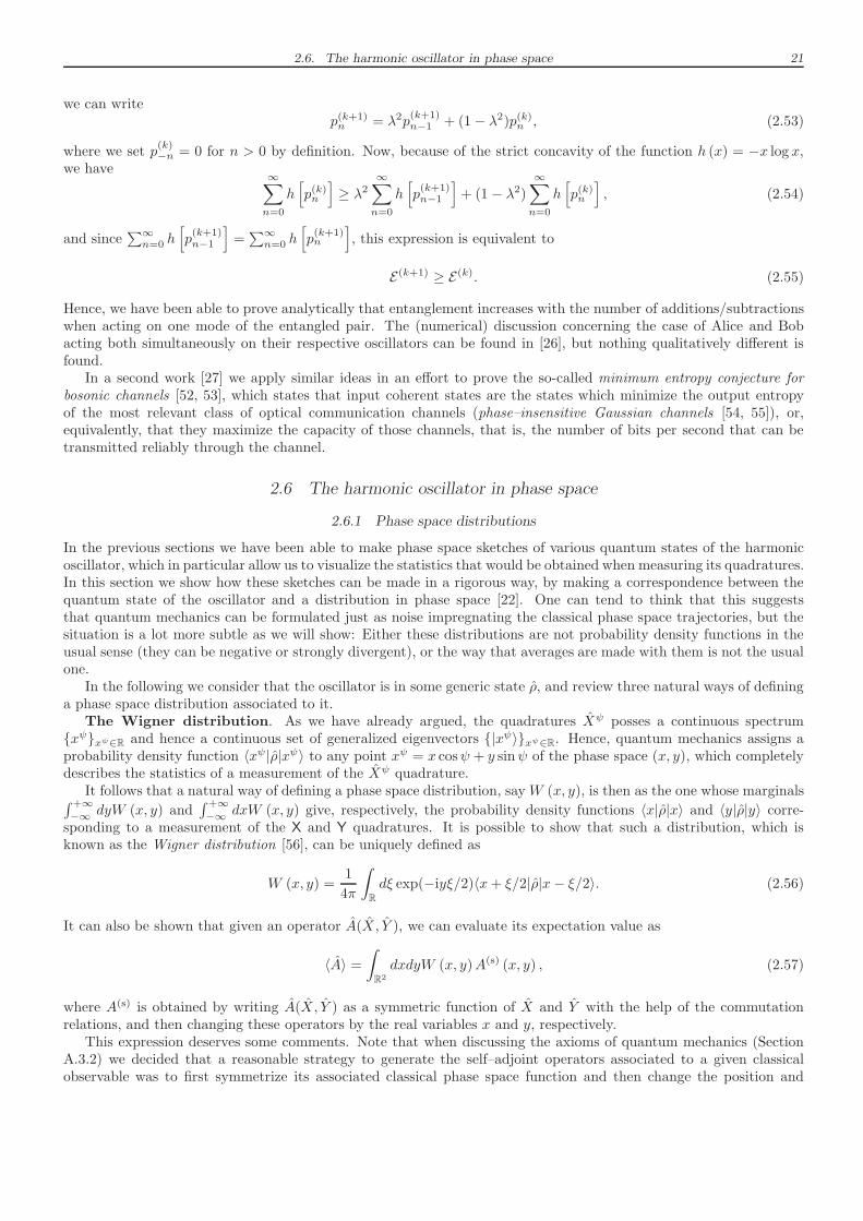
2.6. The harmonic oscillator in phase space 21

we can writep(k+1)n = λ2p

(k+1)n−1 + (1− λ2)p(k)n , (2.53)

where we set p(k)−n = 0 for n > 0 by definition. Now, because of the strict concavity of the function h (x) = −x log x,

we have∞∑

n=0

h[

p(k)n

]

≥ λ2∞∑

n=0

h[

p(k+1)n−1

]

+ (1 − λ2)∞∑

n=0

h[

p(k)n

]

, (2.54)

and since∑∞n=0 h

[

p(k+1)n−1

]

=∑∞n=0 h

[

p(k+1)n

]

, this expression is equivalent to

E(k+1) ≥ E(k). (2.55)

Hence, we have been able to prove analytically that entanglement increases with the number of additions/subtractionswhen acting on one mode of the entangled pair. The (numerical) discussion concerning the case of Alice and Bobacting both simultaneously on their respective oscillators can be found in [26], but nothing qualitatively different isfound.

In a second work [27] we apply similar ideas in an effort to prove the so-called minimum entropy conjecture forbosonic channels [52, 53], which states that input coherent states are the states which minimize the output entropyof the most relevant class of optical communication channels (phase–insensitive Gaussian channels [54, 55]), or,equivalently, that they maximize the capacity of those channels, that is, the number of bits per second that can betransmitted reliably through the channel.

2.6 The harmonic oscillator in phase space

2.6.1 Phase space distributions

In the previous sections we have been able to make phase space sketches of various quantum states of the harmonicoscillator, which in particular allow us to visualize the statistics that would be obtained when measuring its quadratures.In this section we show how these sketches can be made in a rigorous way, by making a correspondence between thequantum state of the oscillator and a distribution in phase space [22]. One can tend to think that this suggeststhat quantum mechanics can be formulated just as noise impregnating the classical phase space trajectories, but thesituation is a lot more subtle as we will show: Either these distributions are not probability density functions in theusual sense (they can be negative or strongly divergent), or the way that averages are made with them is not the usualone.

In the following we consider that the oscillator is in some generic state ρ, and review three natural ways of defininga phase space distribution associated to it.

The Wigner distribution. As we have already argued, the quadratures Xψ posses a continuous spectrumxψxψ∈R and hence a continuous set of generalized eigenvectors |xψ〉xψ∈R. Hence, quantum mechanics assigns aprobability density function 〈xψ|ρ|xψ〉 to any point xψ = x cosψ + y sinψ of the phase space (x, y), which completelydescribes the statistics of a measurement of the Xψ quadrature.

It follows that a natural way of defining a phase space distribution, sayW (x, y), is then as the one whose marginals∫ +∞

−∞dyW (x, y) and

∫ +∞

−∞dxW (x, y) give, respectively, the probability density functions 〈x|ρ|x〉 and 〈y|ρ|y〉 corre-

sponding to a measurement of the X and Y quadratures. It is possible to show that such a distribution, which isknown as the Wigner distribution [56], can be uniquely defined as

W (x, y) =1

4π

∫

R

dξ exp(−iyξ/2)〈x+ ξ/2|ρ|x− ξ/2〉. (2.56)

It can also be shown that given an operator A(X, Y ), we can evaluate its expectation value as

〈A〉 =∫

R2

dxdyW (x, y)A(s) (x, y) , (2.57)

where A(s) is obtained by writing A(X, Y ) as a symmetric function of X and Y with the help of the commutationrelations, and then changing these operators by the real variables x and y, respectively.

This expression deserves some comments. Note that when discussing the axioms of quantum mechanics (SectionA.3.2) we decided that a reasonable strategy to generate the self–adjoint operators associated to a given classicalobservable was to first symmetrize its associated classical phase space function and then change the position and

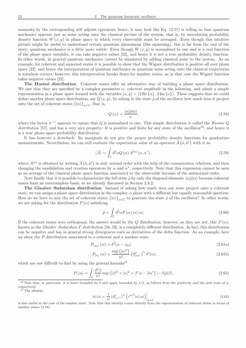
22 2. The quantum harmonic oscillator

momenta by the corresponding self–adjoint operators; hence, it may look like Eq. (2.57) is telling us that quantummechanics appears just as noise acting onto the classical picture of the system, that is, by introducing probabilitydensity function W (x, y) in phase space to which every observable must be averaged. Even though this intuitivepicture might be useful to understand certain quantum phenomena (like squeezing), this is far from the end of thestory; quantum mechanics is a little more subtle: Even though W (x, y) is normalized to one and is a real functionof the phase space variables, it can take negative values [22], and hence it is not a true probability density function.In other words, in general quantum mechanics cannot be simulated by adding classical noise to the system. As anexample, for coherent and squeezed states it is possible to show that the Wigner distribution is positive all over phasespace [22], and hence the interpretation of quantum mechanics as quantum noise acting onto the classical trajectoriesis somehow correct; however, this interpretation breaks down for number states, as in that case the Wigner functiontakes negative values [22].

The Husimi distribution. Coherent states offer an alternative way of building a phase space distribution.We saw that they are specified by a complex parameter α, coherent amplitude in the following, and admit a simplerepresentation in a phase space formed with the variables (x, y) = (2Re α , 2 Im α). These suggests that we coulddefine another phase space distribution, say Q (x, y), by asking to the state ρ of the oscillator how much does it projectonto the set of coherent states |α〉α∈C, that is,

Q (α) =〈α|ρ|α〉π

, (2.58)

where the factor π−1 appears to ensure that Q is normalized to one. This simple distribution is called the Husimi Qdistribution [57], and has a very nice property: It is positive and finite for any state of the oscillator16, and hence itis a true phase space probability distribution.

It has however a drawback: Its marginals do not give the proper probability density functions for quadraturemeasurements. Nevertheless, we can still evaluate the expectation value of an operator A

(

a, a†)

with it as

〈A〉 =∫

C

d2αQ (α)A(a) (α, α∗) , (2.59)

where A(a) is obtained by writing A(

a, a†)

in anti–normal order with the help of the commutation relations, and thenchanging the annihilation and creation operators by α and α∗, respectively. Note that this expression cannot be seenas an average of the classical phase space function associated to the observable because of the antinormal order.

Note finally that it is possible to characterize the full state ρ by only the diagonal elements 〈α|ρ|α〉 because coherentstates form an overcomplete basis, as we already discussed in Section 2.3.2.

The Glauber–Sudarshan distribution. Instead of asking how much does our state project onto a coherentstate, we can assign a phase space distribution in the complex–α plane with a different but equally reasonable question:How do we have to mix the set of coherent states |α〉α∈C to generate the state ρ of the oscillator? In other words,we are asking for the distribution P (α) satisfying

ρ =

∫

C

d2αP (α) |α〉〈α|. (2.60)

If the coherent states were orthogonal, the answer would be the Q distribution; however, as they are not, this P (α),known as the Glauber–Sudarshan P distribution [58, 59], is a completely different distribution. In fact, this distributioncan be negative and has in general strong divergences such as derivatives of the delta function. As an example, herewe show the P distribution associated to a coherent and a number state

P|α0〉 (α) = δ2(α− α0), (2.61a)

P|n〉 (α) =exp

(

|α|2)

n!

(

∂2αα∗

)nδ2(α), (2.61b)

which are not difficult to find by using the general formula17

P (α) =

∫

C

d2β

π2exp

(

|β|2 + |α|2 + β∗α− βα∗)

〈−β|ρ|β〉, (2.63)

16 Note that, in particular, it is lower bounded by 0 and upper bounded by 1/π, as follows from the positivity and the unit trace of ρ,respectively17 The identity

|n〉〈n| =1

n!

(∂2α,α∗

)n(

e|α|2 |α〉〈α|)∣∣∣∣α=0

, (2.62)

is also useful in the case of the number state. Note that this identity comes directly from the representation of coherent states in terms ofnumber states (2.18).

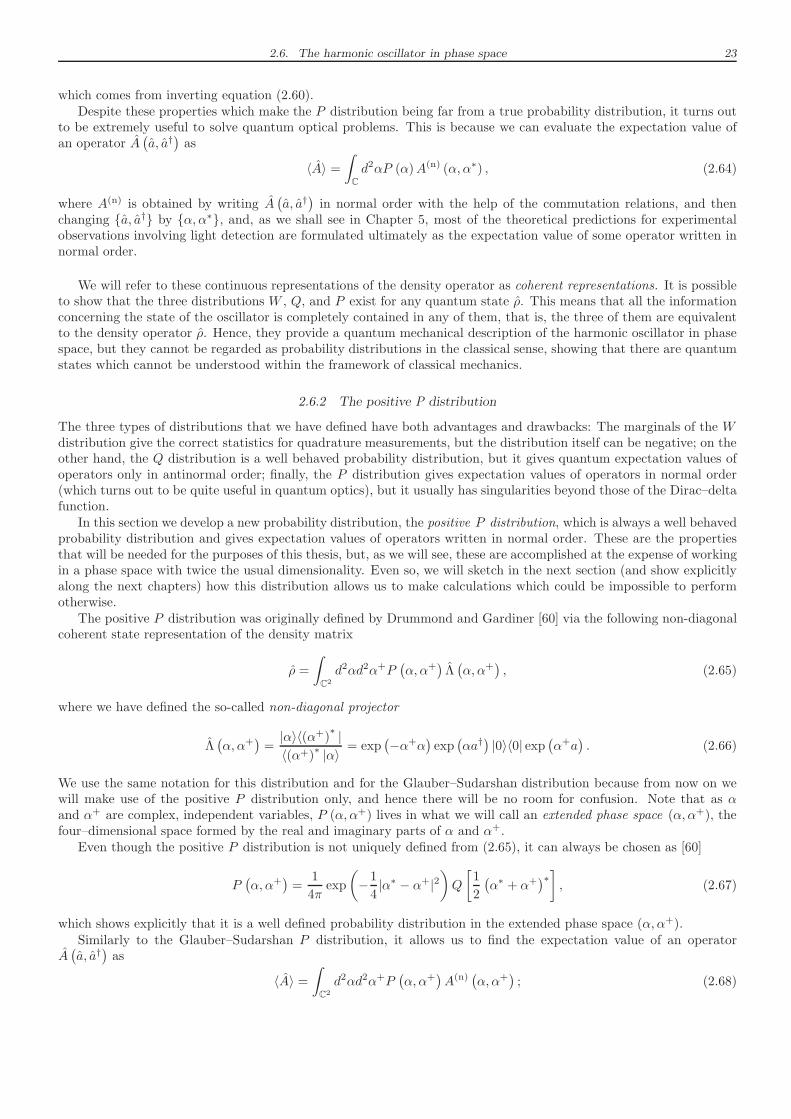
2.6. The harmonic oscillator in phase space 23

which comes from inverting equation (2.60).Despite these properties which make the P distribution being far from a true probability distribution, it turns out

to be extremely useful to solve quantum optical problems. This is because we can evaluate the expectation value ofan operator A

(

a, a†)

as

〈A〉 =∫

C

d2αP (α)A(n) (α, α∗) , (2.64)

where A(n) is obtained by writing A(

a, a†)

in normal order with the help of the commutation relations, and thenchanging a, a† by α, α∗, and, as we shall see in Chapter 5, most of the theoretical predictions for experimentalobservations involving light detection are formulated ultimately as the expectation value of some operator written innormal order.

We will refer to these continuous representations of the density operator as coherent representations. It is possibleto show that the three distributions W , Q, and P exist for any quantum state ρ. This means that all the informationconcerning the state of the oscillator is completely contained in any of them, that is, the three of them are equivalentto the density operator ρ. Hence, they provide a quantum mechanical description of the harmonic oscillator in phasespace, but they cannot be regarded as probability distributions in the classical sense, showing that there are quantumstates which cannot be understood within the framework of classical mechanics.

2.6.2 The positive P distribution

The three types of distributions that we have defined have both advantages and drawbacks: The marginals of the Wdistribution give the correct statistics for quadrature measurements, but the distribution itself can be negative; on theother hand, the Q distribution is a well behaved probability distribution, but it gives quantum expectation values ofoperators only in antinormal order; finally, the P distribution gives expectation values of operators in normal order(which turns out to be quite useful in quantum optics), but it usually has singularities beyond those of the Dirac–deltafunction.

In this section we develop a new probability distribution, the positive P distribution, which is always a well behavedprobability distribution and gives expectation values of operators written in normal order. These are the propertiesthat will be needed for the purposes of this thesis, but, as we will see, these are accomplished at the expense of workingin a phase space with twice the usual dimensionality. Even so, we will sketch in the next section (and show explicitlyalong the next chapters) how this distribution allows us to make calculations which could be impossible to performotherwise.

The positive P distribution was originally defined by Drummond and Gardiner [60] via the following non-diagonalcoherent state representation of the density matrix

ρ =

∫

C2

d2αd2α+P(

α, α+)

Λ(

α, α+)

, (2.65)

where we have defined the so-called non-diagonal projector

Λ(

α, α+)

=|α〉〈(α+)

∗ |〈(α+)

∗ |α〉 = exp(

−α+α)

exp(

αa†)

|0〉〈0| exp(

α+a)

. (2.66)

We use the same notation for this distribution and for the Glauber–Sudarshan distribution because from now on wewill make use of the positive P distribution only, and hence there will be no room for confusion. Note that as αand α+ are complex, independent variables, P (α, α+) lives in what we will call an extended phase space (α, α+), thefour–dimensional space formed by the real and imaginary parts of α and α+.

Even though the positive P distribution is not uniquely defined from (2.65), it can always be chosen as [60]

P(

α, α+)

=1

4πexp

(

−1

4|α∗ − α+|2

)

Q

[

1

2

(

α∗ + α+)∗]

, (2.67)

which shows explicitly that it is a well defined probability distribution in the extended phase space (α, α+).Similarly to the Glauber–Sudarshan P distribution, it allows us to find the expectation value of an operator

A(

a, a†)

as

〈A〉 =∫

C2

d2αd2α+P(

α, α+)

A(n)(

α, α+)

; (2.68)

24 2. The quantum harmonic oscillator

note that the correspondence a† → α∗ in the normal form of the operator A is replaced within this representation bya† → α+.

We would like to finally note that it is completely straightforward to prove that Λ (α, α+) is an analytic function18

of the complex variables (α, α+), while the distribution P (α, α+) itself is not, as it has to depend on both (α, α+) andtheir complex conjugates in order to be a real function. We will exploit the analycity of Λ (α, α+) in the next sectionand along the upcoming chapters.

2.6.3 Fokker–Planck and stochastic Langevin equations

As a taste of the usefulness of the positive P representation, consider the following evolution equation for the state ofan oscillator:

dρ

dt=[

−iωa†a+(

κa†2 − κ∗a2)

+(

E a† − E∗a)

, ρ]

+ γ(

2aρa† − a†aρ− ρa†a)

, (2.71)

being ω, E , κ, and γ some parameters (ω and γ are real). The first term includes the regular Hamiltonian evolution ofthe oscillator, an squeezing term, and a term corresponding to an external driving of the oscillator, while the secondpart cannot be written in Hamiltonian form, and describes damping on the ideal harmonic motion of the oscillator. Inthe forthcoming chapters we will see how these terms arise naturally in the evolution of light contained in an opticalcavity. In any case, let us assume for the moment that the state of the harmonic oscillator is subject to this evolutionequation. We are going to show that it can be reduced to a set of 2 complex differential equations with noise, that is,to a set of stochastic equations [61].

One way to solve these operator equation would be to project it onto a truncated number state basis |0〉, |1〉, ..., |N〉,obtaining then a linear system with N × N variables (the independent elements of the representation of the densityoperator). This method, however, is usually of little help if we intend to deal with states having a large number ofphotons, so that the size of the linear system is too large. It is in this case when coherent representations can beuseful. Let us explain this for the positive P distribution.

We would like to stress that even though we are using equation (2.71) as a guiding example, most of the derivationsthat we are going to perform are completely general.

Let us collect the coherent variables into a single vector α = col(α, α+). It is very simple to prove that thenondiagonal projector Λ (α) satisfies the following properties:

aΛ (α) = αΛ (α) (2.72a)

Λ (α) a =

(

α+∂

∂α+

)

Λ (α) (2.72b)

Λ (α) a† = α+Λ (α) (2.72c)

a†Λ (α) =

(

α+ +∂

∂α

)

Λ (α) ; (2.72d)

therefore, introducing the expansion of the density operator in terms of the positive P distribution (2.65), theseproperties allow us to rewrite the evolution equation (2.71) as

∫

C2

d4αΛ (α) ∂tP (α; t) =

∫

C2

d4αd2α+P (α; t)

∑

j

Aj (α) ∂j +1

2

∑

jl

Djl (α) ∂j∂l

Λ (α) , (2.73)

18 Given the complex function f (z) = fR (zR, zI) + ifI (zR, zI) of a complex variable z = zR + izI, where fR, fI, zR, and zI are allreal, we say that it is analytic if the derivative of the function in the complex–z plane does not depend on the direction along which it isperformed. A necessary and sufficient condition for this is that all the partial derivatives ∂fk/∂zl (k, l = R, I) are continuous and satisfythe Cauchy–Riemann relations

∂fR

∂zR=∂fI

∂zIand

∂fR

∂zI= −

∂fI

∂zR. (2.69)

Note that this relations imply that ∂f/∂z∗ = 0, and hence, an analytical complex function can only depend on zR and zI through thecombination zR + izI, that is, it cannot depend on the complex conjugate of z. An important property of analytical complex functions isthat the derivative respect to the complex variable can be made in two equivalent ways

df

dz=

∂f

∂zR= −i

∂f

∂zI. (2.70)

All this discussion is generalized to a complex function of several complex variables in a natural straightforward manner.

2.6. The harmonic oscillator in phase space 25

where all the indices can take the values α or α+, and

Aα (α) = E − (γ + iω)α+ 2κα+, (2.74a)

Aα+ (α) = E∗ − (γ − iω)α+ + 2κ∗α, (2.74b)

Dαα (α) = 2κ = D∗α+α+ (α) , (2.74c)

Dαα+ (α) = Dα+α (α) = 0. (2.74d)

The symmetric matrix D can always be decomposed as D = BBT for some matrix B, although this is not unique(note that it has to be a 2 × d matrix, though, with d arbitrary). D being diagonal in this particular example, wecould choose for example

B =

[√2κ 0

0√2κ∗

]

. (2.75)

Define now the real and imaginary parts of the coherent amplitudes α = αR + iαI and α+ = α+

R + iα+I , which we

collect in the vectors αR = col(αR, α+R) and αI = col(αI, α

+I ). Define also the real and imaginary parts of the vector

A and the matrix B by

Aj (α) = AjR(αR,αI) + iAjI (αR,αI), (2.76a)

Bjl (α) = BjlR (αR,αI) + iBjlI (αR,αI). (2.76b)

The analyticity of Λ (α) allows us to choose the derivatives ∂j as ∂Rj or −i∂Ij at will, where we use the notation

∂/∂αR = ∂Rα and ∂/∂αI = ∂Iα (similarly for α+), and we choose them so that the differential operator inside thesquare brackets reads

∑

j

(

AjR∂Rj +AjI∂

Ij

)

+1

2

∑

jlm

(

BjmR BlmR ∂Rj ∂Rl + 2BjmR BlmI ∂Rj ∂

Il +BjmI BlmI ∂Ij∂

Il

)

, (2.77)

for future convenience.The main result of the section is obtained by performing an integration by parts in (2.73) to make the derivatives

act onto P (α; t) instead of onto the projector Λ (α), what leads to

∂tP (α; t) =

−∑

j

(

∂Rj AjR + ∂IjA

jI

)

+1

2

∑

jlm

(

∂Rj ∂Rl B

jmR BlmR + 2∂Rj ∂

IlB

jmR BlmI + ∂Ij∂

IlB

jmI BlmI

)

P (α; t) , (2.78)

where we have used the fact that physical states must correspond to positive P distributions which decay to zero atinfinity, so that we can get rid of the total derivative terms appearing upon integrating by parts. Hence, we haveturned the operator equation (2.71) into a linear partial differential equation for the P distribution. Indeed, this

equation is a very special one. By defining the vector ~A = col(AαR, Aα+

R , AαI , Aα+

I ) and the matrix

D =

[

BRBTR BRB

TI

BIBTR BIB

TI

]

= BBT with B =

[

BR 02×2BI 02×2

]

, (2.79)

we can write it in the more compact way

∂tP (x; t) =

−4∑

j=1

∂jAj (x) +1

2

4∑

jl=1

∂j∂lDjl (x)

P (x; t) , (2.80)

where we have defined the vector x = col(αR, α+R , αI, α

+I ). When the matrix D is positive semidefinite, as it is in our

case, this is known as the Fokker–Planck equation [61]; this equation has been subject of study for a very long time,

and we have a lot of different techniques available to solve it or extract information from it. ~A, D, and B, are knownas the drift vector, the diffusion matrix, and the noise matrix, respectively.

For this thesis, the most important property of Fokker–Planck equations is its relation to stochastic equations. Inparticular, it can be proved that any Fokker–Planck equation written in the form (2.80) is equivalent to the followingsystem of stochastic equations [61]

x = ~A (x) + B (x)η (t) , (2.81)

26 2. The quantum harmonic oscillator

where η (t) = col[η1 (t) , η2 (t) , η3 (t) , η4 (t)] is a vector whose elements are independent, real, Gaussian noises whichsatisfy the statistical properties

〈ηj (t)〉 = 0 and 〈ηj (t) ηl (t′)〉 = δjlδ(t− t′). (2.82)

We will call stochastic Langevin equations to these equations. The equivalence between them and the original Fokker–Planck equation must be understood in the “average” sense, that is, given any function F (x), we can find its averageeither by using the distribution P (x; t) or the solutions x[η(t)] of the variables in terms of noise integrals as

∫

R4

d4xF (x)P (x; t) = 〈F x[η(t)]〉 . (2.83)

Given the simple structure of B, see (2.79), we can rewrite the Langevin equations in the complex form

α = A (α) +B (α)η (t) , (2.84)

where η (t) = col[η1 (t) , η2 (t)] is in this case a two–dimensional vector. This is an amazingly simple final result: Ascomplex stochastic variables, α and α+ evolve according to a set of Langevin equations built with the original Aand D = BBT . Then, whenever we are able to rewrite an arbitrary master equation in the form (2.73) by using thepositive P representation, we can directly write down equations (2.84) for the coherent amplitudes of the system.

Applied to our purposes, this means that given the solution α = α[η (t)] of equation (2.84), we can evaluate thequantum expectation value of any operator A

(

a, a†)

as

〈A〉 = 〈A(n)(

α, α+)

〉P , (2.85)

where in the following we will denote by 〈...〉P to any stochastic average obtained from the Langevin equations withinthe positive P representation.

There is one subtlety that we have not mentioned though. Without entering into much detail (see [61] for a deepdiscussion), a stochastic equation can be interpreted in infinitely many inequivalent ways, which attend to how theintegrals involving noise are defined in the Riemann sense, that is, as a limit of some series. The connection we madebetween the Fokker–Planck equation and the Langevin equations is only valid if the stochastic equations are interpretedin a very particular form first defined by Ito (the so-called Ito interpretation). The problem with this interpretationis that integration is defined in such a way that the rules of calculus as we know them no longer apply, and one needsto use a new form of calculus called Ito calculus. Integrals can be defined in a way which allows us to use the usualrules of calculus, arriving then to the so-called Stratonovich interpretation of stochastic equations. However, there is aprice to pay: Interpreted in such way, the set of stochastic equations associated to the Fokker–Planck equation (2.80)is no longer (2.84), but the same type of equation with a different deterministic part given by

A(St)j (α) = Aj (α)− 1

2

∑

lm

Blm (α) ∂lBjm (α) , with j, l,m = α, α+, (2.86)

that is, the deterministic part of the equations acquires an extra term which depends on the noise matrix. In thisthesis we shall always use this Stratonovich form. Nevertheless, note that if the noise matrix does not depend on thecoherent amplitudes α, both forms are the same, that is, Ito and Stratonovich interpretations differ only when noise ismultiplicative, not additive. This is indeed the case in our simple example (2.74,2.75), whose associated set of complexLangevin equations are given by

α = E − (γ + iω)α+ 2κα+ +√2κη1(t), (2.87a)

α+ = E∗ − (γ − iω)α+ + 2κ∗α+√2κ∗η2(t), (2.87b)

both within the Ito and Stratonovich interpretations.

3. QUANTIZATION OF THE ELECTROMAGNETIC FIELDIN AN OPTICAL CAVITY

The goal of this chapter is the quantization of the electromagnetic field inside an optical cavity with perfectly reflectingmirrors. We will follow a heuristic, but physically intuitive approach in which the electromagnetic field is put incorrespondence with a collection of harmonic oscillators. Nevertheless, we would like to note that the quantization ofthe electromagnetic field can be carried out in a more rigorous fashion by generalizing the method that we describedfor mechanical systems in the previous chapter and in Appendix A; this procedure relies on a Lagrangian theory offields, and is called canonical quantization [16].

In order to show how the heuristic procedure works, we will first apply the method to a simple, but highly relevantcase: The quantization of the electromagnetic field in free space. This will allow us to introduce plane–waves as wellas the concept of polarization. We then pass to describe optical beams within the paraxial approximation, and discussthe modal decomposition of such fields in terms of transverse modes. We finally consider the electromagnetic fieldinside a stable optical cavity and proceed to its quantization.

3.1 Light as an electromagnetic wave

Nowadays it feels quite natural to say that light is an electromagnetic wave. Arriving to this conclusion, however, wasnot trivial at all. The history of such a discovery starts in the first half of the XIX century with Faraday, who showedthat the polarization of light can change when subject to a magnetic field; this was the first hint suggesting that therecould be a connection between light and electromagnetism, and he was the first to propose that light could be anelectromagnetic disturbance of some kind, able to propagate without the need of a reference medium. However, thisqualitative idea did not find a rigorous mathematical formulation until the second half of the century, when Maxwelldeveloped a consistent theory of electromagnetism, and showed how the theory was able to predict the existence ofelectromagnetic waves propagating at a speed which was in agreement with the speed measured for light at that time[62]. A couple of decades after his proposal, the existence of electromagnetic waves was experimentally demonstratedby Hertz [63], and the theory of light as an electromagnetic wave found its way towards being accepted.

Our starting point are Maxwell’s equations formulated as partial differential equations for the electric andmagnetic1

vector fields E (r, t) and B (r, t), respectively, where r (t) is the position (time) where (when) the fields are observed.This formulation is due to Heaviside [64], as Maxwell originally proposed his theory in terms of quaternions. Thetheory consists of four equations; the first two are called the homogeneous Maxwell equations and read

∇ ·B = 0 and ∇×E = −∂tB, (3.1)

where ∇ = (∂x, ∂y, ∂z). The other two are called the inhomogeneous Maxwell equations and are written as

∇ ·E = ρ/ε0 and ∇×B = µ0ε0∂tE+ µ0j, (3.2)

where any electric or magnetic source is introduced in the theory by a charge density function ρ (r, t) and a currentdistribution vector j (r, t), respectively; the parameters ε0 = 8.8 × 10−12 F/m and µ0 = 1.3 × 10−6 H/m are theso-called electric permittivity and the magnetic permeability of vacuum, respectively.

We will show the process of quantization of the electromagnetic field in the absence of sources (ρ = 0 and j = 0).Under these circumstances, the inhomogeneous equations are simplified to

∇ · E = 0 and c2∇×B = ∂tE, (3.3)

where c = 1/√ε0µ0 ≃ 3× 108m/s.

The homogeneous equations (3.1) allow us to derive the fields from a scalar potential φ (r, t) and a vector potentialA (r, t) as

B = ∇×A and E = −∇φ− ∂tA, (3.4)

1 As we won’t deal with materials sensitive to the magnetic field, we will use the term “magnetic field” for the B-field, which is usuallydenoted by “magnetic induction field” when it needs to be distinguished from the H-field (which we won’t be using in this thesis).

28 3. Quantization of the electromagnetic field in an optical cavity

hence reducing to four the degrees of freedom of the electromagnetic field. These potentials, however, are not unique;we can always use an arbitrary function Λ (r, t) to change them as

A→ A+∇Λ and φ→ φ− ∂tΛ, (3.5)

what is known as the gauge invariance of Maxwell’s equations.Introducing (3.4) into the inhomogeneous equations we get the equations satisfied by the potentials

(

c2∇2 − ∂2t)

A = ∂t∇φ+ c2∇ (∇ ·A) (3.6a)

∇2φ+ ∂t∇ ·A = 0. (3.6b)

The problem is highly simplified if we exploit the gauge invariance and choose ∇ ·A = 0, as the second equation canbe shown to further imply that φ = 0 for physical fields vanishing at infinity, and hence the only equations left are

(

c2∇2 − ∂2t)

A = 0 (3.7)

which are wave equations with speed c for the components of the vector potential. Note that the condition ∇ ·A = 0(known as the Coulomb condition) relates the three components of A, and hence, only two degrees of freedom of theinitial six (the electric and magnetic vector fields) remain.

It is finally important to note that the wave equation (3.7) has a unique solution inside a given spatio–temporalregion only if both the vector potential and its derivative along the direction normal to the boundary of the regionare specified at any point of the boundary [65]; these are known as Dirichlet and Neumann conditions, respectively.In general, however, physical problems do not impose all those constraints, and hence there coexist several solutionsof the wave equation, which we will call spatio–temporal modes of the system.

In all the optical systems that we will treat, we will be able to write these solutions in the form εA (r, t), with ε

a constant unit vector and A (r, t) a function of space and time; this is called the scalar approximation, and can bemade when the system looks the same for the two independent components of the vector potential (for example, bothcomponents must be subject to the same boundary conditions). In addition, it will be convenient to look for solutionsseparable in space and time, that is, A (r, t) = u (r)A(t). We will see that the connection with the harmonic oscillatoris made through the temporal part of the solutions. As for the spatial part, introducing the separable ansatz in thewave equation, we find that it must satisfy the equation

∇2u+ k2u = 0, (3.8)

where k2 is a suitable separation constant. This is a Helmholtz equation, which yields a unique solution inside agiven volume only if the Dirichlet or Neumann conditions are given for u(r) [65]. If the boundary conditions areless restrictive than these, several solutions un(r) appear corresponding to the eigenfunctions of the differentialoperator ∇

2, which is a self–adjoint differential operator called Laplacian, whose corresponding eigenvalues −k2ncan be shown to be all negative. These solutions are known as the spatial modes of the system, and play a central rolein the heuristic quantization procedure that we will follow.

3.2 Quantization in free space: Plane waves and polarization

3.2.1 Quantization in terms of plane waves

The scalar approximation works fine in free space, as by definition it has no boundaries. This also means that theHelmholtz equation (3.8) has to be solved in all R3. In this case, the eigenfunctions of the Laplacian form a continuousset given by exp (ik · r)k∈R3, with corresponding eigenvalues −|k|2k∈R3. Hence, the solutions of the wave equationwill be of the type ε (k)A(k, t) exp (ik · r). Moreover, the Coulomb condition imposes that k · ε (k) = 0, that is, thevector potential is orthogonal to the mode vectors k; this means that for any k we can define two vectors ε1 (k) andε2 (k), which are called the polarization vectors, satisfying the relations

k · εσ (k) = 0, (σ = 1, 2) (3.9a)

ε∗σ (k) · εσ′ (k) = δσσ′ , (σ, σ′ = 1, 2) (3.9b)

ε∗1 (k) × ε2 (k) = k/k ≡ κ, (3.9c)

with k = |k|, so that we can make the following modal expansion of the vector potential:

A (r, t) =∑

σ=1,2

∫

R3

d3kεσ (k)Aσ(k, t) exp (ik · r) . (3.10)

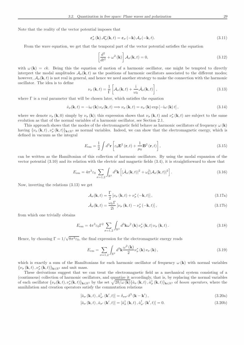
3.2. Quantization in free space: Plane waves and polarization 29

Note that the reality of the vector potential imposes that

ε∗σ (k)A∗σ(k, t) = εσ (−k)Aσ(−k, t). (3.11)

From the wave equation, we get that the temporal part of the vector potential satisfies the equation

[

d2

dt2+ ω2 (k)

]

Aσ(k, t) = 0, (3.12)

with ω (k) = ck. Being this the equation of motion of a harmonic oscillator, one might be tempted to directlyinterpret the modal amplitudes Aσ(k, t) as the positions of harmonic oscillators associated to the different modes;however, Aσ(k, t) is not real in general, and hence we need another strategy to make the connection with the harmonicoscillator. The idea is to define

νσ (k, t) =1

Γ

[

Aσ(k, t) +i

ωkAσ(k, t)

]

, (3.13)

where Γ is a real parameter that will be chosen later, which satisfies the equation

νσ(k, t) = −iω (k) νσ(k, t) =⇒ νσ (k, t) = νσ (k) exp [−iω (k) t] , (3.14)

where we denote νσ (k, 0) simply by νσ (k); this expression shows that νσ (k, t) and ν∗σ (k, t) are subject to the same

evolution as that of the normal variables of a harmonic oscillator, see Section 2.1.This approach shows that the modes of the electromagnetic field behave as harmonic oscillators of frequency ω (k)

having νσ (k, t) , ν∗σ (k, t)k∈R3 as normal variables. Indeed, we can show that the electromagnetic energy, which isdefined in vacuum as the integral

Eem =1

2

∫

d3r

[

ε0E2 (r, t) +

1

µ0B2 (r, t)

]

, (3.15)

can be written as the Hamiltonian of this collection of harmonic oscillators. By using the modal expansion of thevector potential (3.10) and its relation with the electric and magnetic fields (3.4), it is straightforward to show that

Eem = 4π3ε0∑

σ=1,2

∫

R3

d3k[

|Aσ(k, t)|2 + ω2k|Aσ(k, t)|2

]

. (3.16)

Now, inverting the relations (3.13) we get

Aσ(k, t) =Γ

2[νσ (k, t) + ν∗σ (−k, t)] , (3.17a)

Aσ(k, t) =ωkΓ

2i[νσ (k, t)− ν∗σ (−k, t)] , (3.17b)

from which one trivially obtains

Eem = 4π3ε0Γ2∑

σ=1,2

∫

R3

d3kω2 (k) ν∗σ (k, t) νσ (k, t) . (3.18)

Hence, by choosing Γ = 1/√8π3ε0, the final expression for the electromagnetic energy reads

Eem =∑

σ=1,2

∫

R3

d3kω2 (k)

2ν∗σ (k) νσ (k) , (3.19)

which is exactly a sum of the Hamiltonians for each harmonic oscillator of frequency ω (k) with normal variablesνσ (k, t) , ν∗σ (k, t)k∈R3 and unit mass.

These derivations suggest that we can treat the electromagnetic field as a mechanical system consisting of a(continuous) collection of harmonic oscillators, and quantize it accordingly, that is, by replacing the normal variablesof each oscillator νσ(k, t), ν∗σ(k, t)k∈R3 by the set

√

2~/ω (k)aσ (k, t) , a†σ (k, t)k∈R3 of boson operators, where theannihilation and creation operators satisfy the commutation relations

[aσ (k, t) , a†σ′ (k

′, t)] = δσσ′δ3 (k− k′) , (3.20a)

[aσ (k, t) , aσ′ (k′, t)] = [a†σ (k, t) , a†σ′ (k

′, t)] = 0. (3.20b)

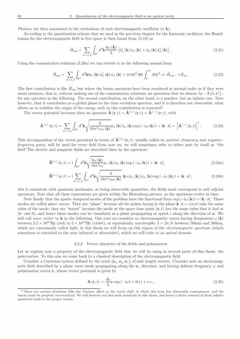
30 3. Quantization of the electromagnetic field in an optical cavity

Photons are then associated to the excitations of each electromagnetic oscillator (σ,k).According to the quantization scheme that we used in the previous chapter for the harmonic oscillator, the Hamil-

tonian for the electromagnetic field in free space is then found from (3.19) as

Hem =∑

σ=1,2

∫

R3

d3k~ω (k)

2

[

a†σ (k) aσ (k) + aσ (k) a†σ (k)

]

. (3.21)

Using the commutation relations (3.20a) we can rewrite it in the following normal form

Hem =∑

σ=1,2

∫

R3

d3k~ω (k) a†σ (k) aσ (k) + 4π~δ3 (0)

∫ ∞

0

dkk3 ≡: Hem : +E∞. (3.22)

The first contribution is like Hem but where the boson operators have been reordered in normal order as if they wereusual numbers, that is, without making use of the commutation relations, an operation that we denote by : A

(

a, a†)

:for any operator in the following. The second contribution, on the other hand, is a number, but an infinite one. Notehowever, that it contributes as a global phase to the time evolution operator, and it is therefore not observable, whatallows us to redefine the origin of the energy such as this contribution is removed2.

The vector potential becomes then an operator A (r, t) = A(+) (r, t) + A(−) (r, t), with

A(+) (r, t) =∑

σ=1,2

∫

R3

d3k

√

~

16π3ε0ω (k)εσ (k) aσ (k) exp [−iω (k) t+ ik · r] =

[

A(−) (r, t)]†

. (3.23)

This decomposition of the vector potential in terms of A(±) (r, t), usually called its positive–frequency and negative–frequency parts, will be used for every field from now on; we will sometimes refer to either part by itself as “thefield”The electric and magnetic fields are described then by the operators

E(+) (r, t) = i

∫

R3

d3k

√

~ω (k)

16π3ε0εσ (k) aσ (k) exp [−iω (k) t+ ik · r] , (3.24a)

B(+) (r, t) = i∑

σ=1,2

∫

R3

d3k

√

~

16π3ε0ω (k)[k×εσ (k)] aσ (k) exp [−iω (k) t+ ik · r] ; (3.24b)

this is consistent with quantum mechanics, as being observable quantities, the fields must correspond to self–adjointoperators. Note that all these expressions are given within the Heisenberg picture, as the operators evolve in time.

Note finally that the spatio–temporal modes of the problem have the functional form exp [−iω (k) t+ ik · r]. Thesemodes are called plane–waves. They are “plane” because all the points laying in the plane k · r = const take the samevalue of the mode; they are “waves” because the mode at the space time point (r, t) has the same value that it had at(r−cκt, 0), and hence these modes can be visualized as a plane propagating at speed c along the direction of κ. Wewill call wave vector to k in the following. Our eyes are sensitive to electromagnetic waves having frequencies ω (k)between 2.5× 1015Hz (red) to 5× 1015Hz (violet), or equivalently wavelengths λ = 2π/k between 760nm and 380nm,which are customarily called light ; in this thesis we will focus on this region of the electromagnetic spectrum (whichsometimes is extended to the near infrared or ultraviolet), which we will refer to as optical domain.

3.2.2 Vector character of the fields and polarization

Let us explain now a property of the electromagnetic field that we will be using in several parts of this thesis, thepolarization. To this aim we come back to a classical description of the electromagnetic field.

Consider a Cartesian system defined by the triad ex, ey, ez of unit length vectors. Consider now an electromag-netic field described by a plane–wave mode propagating along the ez direction, and having definite frequency ω andpolarization vector ε, whose vector potential is given by

A (r, t) =A0

2ε exp (−iωt+ ikz) + c.c., (3.25)

2 There are certain situations (like the Casimir effect or the Lamb shift) in which this term has observable consequences, and thetheory must be properly renormalized. We will however not find such situations in this thesis, and hence a direct removal of these infinitequantities leads to the proper results.

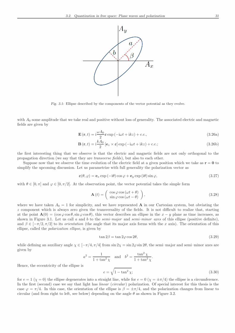
3.2. Quantization in free space: Plane waves and polarization 31

Fig. 3.1: Ellipse described by the components of the vector potential as they evolve.

with A0 some amplitude that we take real and positive without loss of generality. The associated electric and magneticfields are given by

E (r, t) = iωA0

2ε exp (−iωt+ ikz) + c.c., (3.26a)

B (r, t) = ikA0

2[ez × ε] exp (−iωt+ ikz) + c.c.; (3.26b)

the first interesting thing that we observe is that the electric and magnetic fields are not only orthogonal to thepropagation direction (we say that they are transverse fields), but also to each other.

Suppose now that we observe the time evolution of the electric field at a given position which we take as r = 0 tosimplify the upcoming discussion. Let us parametrize with full generality the polarization vector as

ε(θ, ϕ) = ex exp (−iθ) cosϕ+ ey exp (iθ) sinϕ, (3.27)

with θ ∈ [0, π] and ϕ ∈ [0, π/2]. At the observation point, the vector potential takes the simple form

A (t) =

(

cosϕ cos (ωt+ θ)sinϕ cos (ωt− θ)

)

, (3.28)

where we have taken A0 = 1 for simplicity, and we have represented A in our Cartesian system, but obviating thez component which is always zero given the transversality of the fields. It is not difficult to realize that, startingat the point A(0) = (cosϕ cos θ, sinϕ cos θ), this vector describes an ellipse in the x − y plane as time increases, asshown in Figure 3.1. Let us call a and b to the semi–major and semi–minor axes of this ellipse (positive definite),and β ∈ [−π/2, π/2] to its orientation (the angle that its major axis forms with the x axis). The orientation of thisellipse, called the polarization ellipse, is given by

tan 2β = tan 2ϕ cos 2θ, (3.29)

while defining an auxiliary angle χ ∈ [−π/4, π/4] from sin 2χ = sin 2ϕ sin 2θ, the semi–major and semi–minor axes aregiven by

a2 =1

1 + tan2 χand b2 =

tan2 χ

1 + tan2 χ.

Hence, the eccentricity of the ellipse is

e =

√

1− tan2 χ; (3.30)

for e = 1 (χ = 0) the ellipse degenerates into a straight line, while for e = 0 (χ = ±π/4) the ellipse is a circumference.In the first (second) case we say that light has linear (circular) polarization. Of special interest for this thesis is thecase ϕ = π/4. In this case, the orientation of the ellipse is β = ±π/4, and the polarization changes from linear tocircular (and from right to left, see below) depending on the angle θ as shown in Figure 3.2.

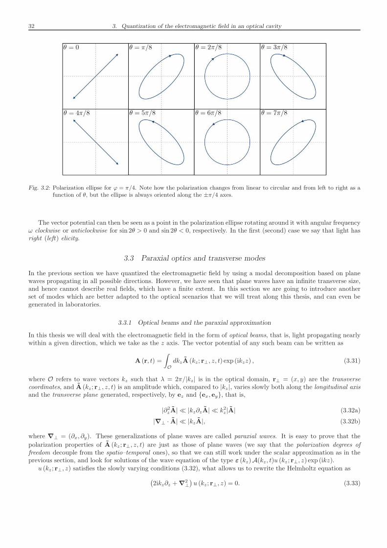
32 3. Quantization of the electromagnetic field in an optical cavity

Fig. 3.2: Polarization ellipse for ϕ = π/4. Note how the polarization changes from linear to circular and from left to right as afunction of θ, but the ellipse is always oriented along the ±π/4 axes.

The vector potential can then be seen as a point in the polarization ellipse rotating around it with angular frequencyω clockwise or anticlockwise for sin 2θ > 0 and sin 2θ < 0, respectively. In the first (second) case we say that light hasright (left) elicity.

3.3 Paraxial optics and transverse modes

In the previous section we have quantized the electromagnetic field by using a modal decomposition based on planewaves propagating in all possible directions. However, we have seen that plane waves have an infinite transverse size,and hence cannot describe real fields, which have a finite extent. In this section we are going to introduce anotherset of modes which are better adapted to the optical scenarios that we will treat along this thesis, and can even begenerated in laboratories.

3.3.1 Optical beams and the paraxial approximation

In this thesis we will deal with the electromagnetic field in the form of optical beams, that is, light propagating nearlywithin a given direction, which we take as the z axis. The vector potential of any such beam can be written as

A (r, t) =

∫

O

dkzA (kz; r⊥, z, t) exp (ikzz) , (3.31)

where O refers to wave vectors kz such that λ = 2π/|kz| is in the optical domain, r⊥ = (x, y) are the transversecoordinates, and A (kz; r⊥, z, t) is an amplitude which, compared to |kz |, varies slowly both along the longitudinal axisand the transverse plane generated, respectively, by ez and ex, ey, that is,

|∂2zA| ≪ |kz∂zA| ≪ k2z |A| (3.32a)

|∇⊥ · A| ≪ |kzA|, (3.32b)

where ∇⊥ = (∂x, ∂y). These generalizations of plane waves are called paraxial waves. It is easy to prove that the

polarization properties of A (kz ; r⊥, z, t) are just as those of plane waves (we say that the polarization degrees offreedom decouple from the spatio–temporal ones), so that we can still work under the scalar approximation as in theprevious section, and look for solutions of the wave equation of the type ε (kz)A(kz , t)u (kz ; r⊥, z) exp (ikz).

u (kz; r⊥, z) satisfies the slowly varying conditions (3.32), what allows us to rewrite the Helmholtz equation as

(

2ikz∂z +∇2⊥

)

u (kz; r⊥, z) = 0. (3.33)

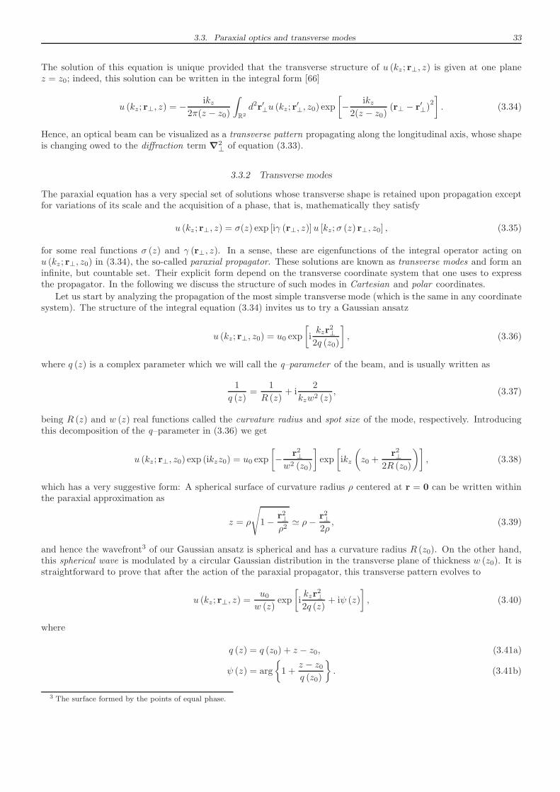
3.3. Paraxial optics and transverse modes 33

The solution of this equation is unique provided that the transverse structure of u (kz ; r⊥, z) is given at one planez = z0; indeed, this solution can be written in the integral form [66]

u (kz; r⊥, z) = −ikz

2π(z − z0)

∫

R2

d2r′⊥u (kz; r′⊥, z0) exp

[

− ikz2(z − z0)

(r⊥ − r′⊥)2]

. (3.34)

Hence, an optical beam can be visualized as a transverse pattern propagating along the longitudinal axis, whose shapeis changing owed to the diffraction term ∇

2⊥ of equation (3.33).

3.3.2 Transverse modes

The paraxial equation has a very special set of solutions whose transverse shape is retained upon propagation exceptfor variations of its scale and the acquisition of a phase, that is, mathematically they satisfy

u (kz ; r⊥, z) = σ(z) exp [iγ (r⊥, z)]u [kz;σ (z) r⊥, z0] , (3.35)

for some real functions σ (z) and γ (r⊥, z). In a sense, these are eigenfunctions of the integral operator acting onu (kz ; r⊥, z0) in (3.34), the so-called paraxial propagator. These solutions are known as transverse modes and form aninfinite, but countable set. Their explicit form depend on the transverse coordinate system that one uses to expressthe propagator. In the following we discuss the structure of such modes in Cartesian and polar coordinates.

Let us start by analyzing the propagation of the most simple transverse mode (which is the same in any coordinatesystem). The structure of the integral equation (3.34) invites us to try a Gaussian ansatz

u (kz; r⊥, z0) = u0 exp

[

ikzr

2⊥

2q (z0)

]

, (3.36)

where q (z) is a complex parameter which we will call the q–parameter of the beam, and is usually written as

1

q (z)=

1

R (z)+ i

2

kzw2 (z), (3.37)

being R (z) and w (z) real functions called the curvature radius and spot size of the mode, respectively. Introducingthis decomposition of the q–parameter in (3.36) we get

u (kz; r⊥, z0) exp (ikzz0) = u0 exp

[

− r2⊥w2 (z0)

]

exp

[

ikz

(

z0 +r2⊥

2R (z0)

)]

, (3.38)

which has a very suggestive form: A spherical surface of curvature radius ρ centered at r = 0 can be written withinthe paraxial approximation as

z = ρ

√

1− r2⊥ρ2≃ ρ− r2⊥

2ρ, (3.39)

and hence the wavefront3 of our Gaussian ansatz is spherical and has a curvature radius R (z0). On the other hand,this spherical wave is modulated by a circular Gaussian distribution in the transverse plane of thickness w (z0). It isstraightforward to prove that after the action of the paraxial propagator, this transverse pattern evolves to

u (kz ; r⊥, z) =u0w (z)

exp

[

ikzr

2⊥

2q (z)+ iψ (z)

]

, (3.40)

where

q (z) = q (z0) + z − z0, (3.41a)

ψ (z) = arg

1 +z − z0q (z0)

. (3.41b)

3 The surface formed by the points of equal phase.

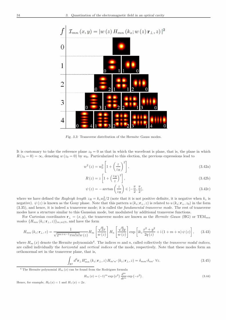
34 3. Quantization of the electromagnetic field in an optical cavity

Fig. 3.3: Transverse distribution of the Hermite–Gauss modes.

It is customary to take the reference plane z0 = 0 as that in which the wavefront is plane, that is, the plane in whichR (z0 = 0) =∞, denoting w (z0 = 0) by w0. Particularized to this election, the previous expressions lead to

w2 (z) = w20

[

1 +

(

z

zR

)2]

, (3.42a)

R (z) = z

[

1 +(zRz

)2]

, (3.42b)

ψ (z) = − arctan

(

z

zR

)

∈ [−π2,π

2], (3.42c)

where we have defined the Rayleigh length zR = kzw20/2 (note that it is not positive definite, it is negative when kz is

negative). ψ (z) is known as the Gouy phase. Note that this pattern u (kz; r⊥, z) is related to u (kz; r⊥, z0) in the form(3.35), and hence, it is indeed a transverse mode; it is called the fundamental transverse mode. The rest of transversemodes have a structure similar to this Gaussian mode, but modulated by additional transverse functions.

For Cartesian coordinates r⊥ = (x, y), the transverse modes are known as the Hermite–Gauss (HG) or TEMmn

modes Hmn (kz; r⊥, z)m,n∈N, and have the form

Hmn (kz ; r⊥, z) =1√

2m+n−1πm!n!w (z)Hm

[ √2x

w (z)

]

Hn

[ √2y

w (z)

]

exp

[

ikzx2 + y2

2q (z)+ i (1 +m+ n)ψ (z)

]

, (3.43)

where Hm (x) denote the Hermite polynomials4. The indices m and n, called collectively the transverse modal indices,are called individually the horizontal and vertical indices of the mode, respectively. Note that these modes form anorthonormal set in the transverse plane, that is,

∫

R2

d2r⊥H∗mn (kz; r⊥, z)Hm′n′ (kz ; r⊥, z) = δmm′δnn′ ∀z. (3.45)

4 The Hermite polynomial Hm (x) can be found from the Rodrigues formula

Hm (x) = (−1)m exp(x2

) dm

dtmexp

(−x2

). (3.44)

Hence, for example, H0 (x) = 1 and H1 (x) = 2x.

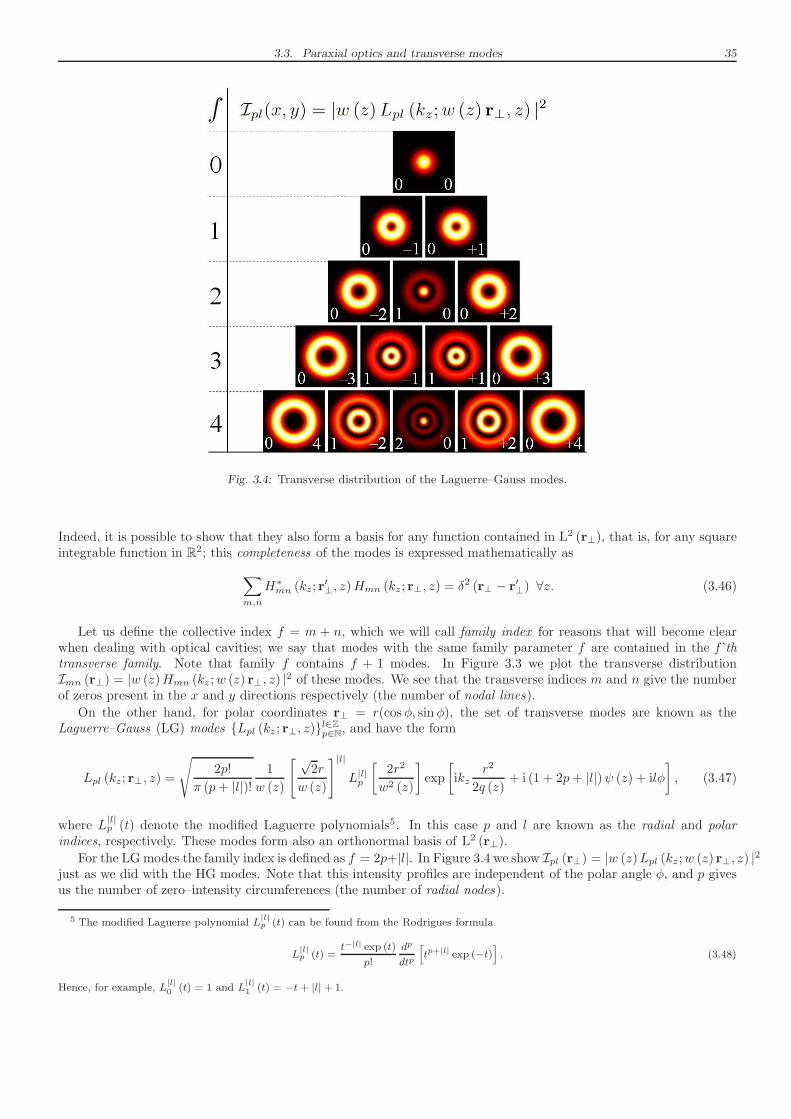
3.3. Paraxial optics and transverse modes 35

Fig. 3.4: Transverse distribution of the Laguerre–Gauss modes.

Indeed, it is possible to show that they also form a basis for any function contained in L2 (r⊥), that is, for any squareintegrable function in R

2; this completeness of the modes is expressed mathematically as

∑

m,n

H∗mn (kz; r′⊥, z)Hmn (kz; r⊥, z) = δ2 (r⊥ − r′⊥) ∀z. (3.46)

Let us define the collective index f = m + n, which we will call family index for reasons that will become clearwhen dealing with optical cavities; we say that modes with the same family parameter f are contained in the f ’thtransverse family. Note that family f contains f + 1 modes. In Figure 3.3 we plot the transverse distributionImn (r⊥) = |w (z)Hmn (kz ;w (z) r⊥, z) |2 of these modes. We see that the transverse indices m and n give the numberof zeros present in the x and y directions respectively (the number of nodal lines).

On the other hand, for polar coordinates r⊥ = r(cosφ, sin φ), the set of transverse modes are known as theLaguerre–Gauss (LG) modes Lpl (kz ; r⊥, z)l∈Zp∈N, and have the form

Lpl (kz; r⊥, z) =

√

2p!

π (p+ |l|)!1

w (z)

[ √2r

w (z)

]|l|

L|l|p

[

2r2

w2 (z)

]

exp

[

ikzr2

2q (z)+ i (1 + 2p+ |l|)ψ (z) + ilφ

]

, (3.47)

where L|l|p (t) denote the modified Laguerre polynomials5. In this case p and l are known as the radial and polar

indices, respectively. These modes form also an orthonormal basis of L2 (r⊥).

For the LGmodes the family index is defined as f = 2p+|l|. In Figure 3.4 we show Ipl (r⊥) = |w (z)Lpl (kz;w (z) r⊥, z) |2just as we did with the HG modes. Note that this intensity profiles are independent of the polar angle φ, and p givesus the number of zero–intensity circumferences (the number of radial nodes).

5 The modified Laguerre polynomial L|l|p (t) can be found from the Rodrigues formula

L|l|p (t) =

t−|l| exp (t)

p!

dp

dtp

[

tp+|l| exp (−t)]

. (3.48)

Hence, for example, L|l|0 (t) = 1 and L

|l|1 (t) = −t+ |l|+ 1.

36 3. Quantization of the electromagnetic field in an optical cavity

Fig. 3.5: Transverse distribution of the Hybrid Laguerre–Gauss modes. Note that the modes of its first family are the same asthe corresponding Hermite–Gauss modes.

Instead of the LG modes which have a complex dependence exp (ilφ) on the polar angle, sometimes it is moreconvenient to use the Hybrid Laguerre–Gauss (HLG) modes Y jpl (kz; r⊥, z)

j=c,sp,l∈N, which are defined as

Ycpl (kz; r⊥, z) =1√2[Lpl (kz; r⊥, z) + Lp,−l (kz ; r⊥, z)] ∝ cos (lφ) , (3.49a)

Yspl (kz; r⊥, z) =1√2i

[Lpl (kz ; r⊥, z)− Lp,−l (kz; r⊥, z)] ∝ sin (lφ) , (3.49b)

and have a trigonometric dependence on φ. Of course, these relations are not valid for l = 0, where the polardependence disappears and the convention is to define the Hybrid cosine mode as the LG mode and the Hybrid sinemode as zero, that is, Ycp0 (kz; r⊥, z) = Lp0 (kz; r⊥, z) and Ysp0 (kz ; r⊥, z) = 0. In Figure 3.5 we show the intensityof these modes. Note that they are like the LG modes, but modulated by a periodic function of the polar angle; inparticular, given the dependence cos (lφ) or sin (lφ), 2l gives the number of zeros present in any circle around r = 0(the number of polar nodes). This set of transverse modes is usually denoted by TEM∗pl in the literature.

In the following, in order to make the next derivations general, we define an arbitrary set of transverse modesTn (kz; r⊥, z)n satisfying the orthonormality and completeness relations

∫

R2

d2r⊥T∗n (kz; r⊥, z)Tn′ (kz; r⊥, z) = δnn′ , (3.50a)

∑

n

T ∗n (kz ; r′⊥, z)Tn (kz; r⊥, z) = δ2 (r⊥ − r′⊥) ∀z; (3.50b)

for example, when the modes are taken to be the HG, LG, or HLG, the set of transverse modal indices n isn,mn,m∈N, p, ll∈Zp∈N, and j, p, l

j=c,sp,l∈N, respectively.

As for arbitrary q (z) and ψ (z) parameters the transverse modes form a basis of L2 (r⊥), which is the space ofphysical transverse patterns (they cannot extend to infinity or have singularities), the vector potential associated toany optical beam propagating along the z axis can be expanded as

A (r, t) =∑

σ=1,2

∑

n

∫

O

dkzεσn (kz)Aσn(kz , t)Tn (kz; r⊥, z) exp (ikzz) . (3.51)

3.4. Quantization in an optical cavity 37

The HG, LG, and HLG modes satisfy the relations

H∗mn (kz ; r⊥, z) = Hmn (−kz; r⊥, z) , (3.52a)

L∗pl (kz ; r⊥, z) = Lp,−l (−kz; r⊥, z) , (3.52b)

Y ∗jpl (kz ; r⊥, z) = Yjpl (−kz; r⊥, z) ; (3.52c)

hence, similarly to what happened with plane waves, the reality of the vector potential imposes the following restrictionson the polarization and temporal parts of the modes:

ε∗σmn (kz)A∗σmn(kz , t) = εσmn (−kz)Aσmn(−kz, t), (3.53a)

ε∗σpl (kz)A∗σpl(kz , t) = εσp,−l (−kz)Aσp,−l(−kz, t), (3.53b)

ε∗σjpl (kz)A∗σjpl(kz , t) = εσjpl (−kz)Aσjpl(−kz , t). (3.53c)

Note finally that all these transverse bases have two free parameters, e.g., the spot size at the waist plane and theposition of this plane; in free space we can choose these parameters as we feel more convenient, and hence this paraxialbasis is actually a continuous family of bases. We will see that these transverse modes form also a basis for lightcontained in an optical cavity, but in this case the parameters of the basis get fixed by the cavity geometry.

3.4 Quantization in an optical cavity

3.4.1 Geometrical optics: Propagation through optical elements and stable optical cavities

Optical cavities are useful for their ability to trap light. In their most basic configuration, they consist on two sphericalmirrors facing each other (linear resonators), so that when an optical beam enters the system, it stays bouncing backand forth between these. In this section we explain the conditions that any cavity must satisfy in order to truly confinelight.

Consider an optical beam propagating nearly within the z axis. In the preceding section we studied the propagationof such a beam by taking into account the diffraction effects of the wave equation. There is yet another description ofthe beam which is very useful owed to its simplicity, but works only for large Fresnel numbers F = d2/λl, where d isthe transverse size of the beam and l the distance that it has propagated along the z axis. This approach is known asgeometrical optics, and it visualizes the beam as a collection of collimated rays propagating as straight lines (hence,it doesn’t take into account the changes in transverse size or shape of the beam). Within this description, any ray isspecified at a given longitudinal position z by a vector

v (z) =

[

r (z)θ (z)

]

, (3.54)

being r (z) its distance to the z axis and θ(z) the angle that it forms with the this axis as it propagates. We will calltransverse position and inclination to these ray coordinates.

The effect of optical elements on the beam is described within this framework by a so-called ABCD matrix

M =

[

A BC D

]

, (3.55)

which takes a ray v (zin) = col(r, θ) of the beam at its input and transforms it into the ray

v (zout) =Mv (zin) =

[

Ar +BθCr +Dθ

]

. (3.56)

The most simple optical operation consists on allowing the beam to propagate in free space a distance l. The resultingABCD matrix is trivially found to be

Mfree (l) =

[

1 l0 1

]

, (3.57)

that is, the inclination of the rays doesn’t change, while their transverse positions are increased by lθ. Another exampleconsists in a spherical interface with curvature radius6 R separating two dielectric media with refractive indices7 nL

6 Some comments on sign conventions are in order. First, optical elements are described as seen from the ray. The curvature radius ofconvex (concave) dielectric surfaces is then taken as positive (negative), and the opposite for reflecting surfaces.

7 The refractive index is rigorously introduced in Chapter 4.

38 3. Quantization of the electromagnetic field in an optical cavity

and nR (assumed propagation from left to right); by using Snell’s law in paraxial form nLθL = nRθR and simplegeometrical arguments, it is straightforward to prove that its ABCD matrix is

Minterface (nL, nR, R) =

[

1 0nL−nRnR

1R

nLnR

]

, (3.58)

that is, in this case the transverse positions of the rays do not change, while their inclination does.From these two fundamental ABCD systems (propagation and refraction) one can find the ABCD matrices of a

whole family of useful optical elements such as thin lenses or mirrors, which have

Mlens (f) =

[

1 0− 1f 1

]

and Mmirror (R) =

[

1 0− 2R 1

]

, (3.59)

where f is called the focal length of the lens and R is the curvature radius of the mirror.Given a general ABCD matrix M connecting two planes with refractive indices nin and nout, one has detM =

nin/nout; to prove this just note that M can always be decomposed as a combination of propagation (3.57) andrefraction (3.58) ABCD matrices, and that the determinant of a product of matrices equals the product of theindividual determinants.

It is very interesting to note that the transverse modes that we just described in the previous section preserve theirtransverse shape upon propagation through an arbitrary ABCD system. In particular, it can be proved that if wetake an arbitrary transverse mode with q–parameter q (zin) and Gouy phase ψ (zin) at the input face of the ABCDsystem, it is transformed at the output face of the optical system into the exact same mode but with new parameters

q (zout) =Aq (zin) +B

Cq (zin) +D, (3.60a)

ψ (zout) = ψ (zin)− arg

A+|B|

q (zin)

; (3.60b)

these expressions are known as the ABCD propagation laws.Let us now pass to describe optical cavities from this geometrical viewpoint. Consider a ray v (z0) = col(r, θ) at

some reference plane z = z0 of the cavity; after a roundtrip inside the cavity, it is transformed by an ABCD matrixthat we will call

Mroundtrip =

[

Art Brt

Crt Drt

]

, (3.61)

which consists in the composition of all the operations performed by the optical elements inside the cavity until theray comes back to the reference plane z = z0 with the same propagation direction (hence detMroundtrip = 1). AfterN roundtrips the ray coordinates will become

vN (z0) =MNroundtripv (z0) =

1

sin θ

[

Art sinNθ − sin [(N − 1) θ] Brt sinNθCrt sinNθ Drt sinNθ − sin (N − 1) θ

]

v (z0) , (3.62)

with cos θ = (Art +Drt)/2, where the second equality comes from the Sylvester theorem applied to the N ’th powerof a 2 × 2 matrix with determinant one. The ray will stay confined in the cavity only if θ is real, as otherwise thetrigonometric functions become hyperbolic, and the ray coordinates diverge. This means that the condition for aresonator to confine optical beams is

− 1 <Art +Drt

2< 1 (3.63)

An optical cavity satisfying this condition is said to be stable. Note that it looks like this condition may depend onthe reference plane from which the roundtrip matrix is evaluated; however, it is possible to show that the trace of theroundtrip matrix does not depend on the reference plane.

As stated, in this thesis we assume that the optical cavity consists in two spherical mirrors with curvature radii R1

and R2 separated a distance L; for reasons that will become clear in Chapter 6, we allow for the existence of a planedielectric slab of length lc and refractive index nc. Taking the reference plane at mirror one with the rays propagatingaway from it, the roundtrip ABCD matrix of this simple cavity is easily found to be

Mroundtrip =

[

2g2 − 1 2g2Leff

2 (2g1g2 − g2 − g1) /Leff 4g1g2 − 2g2 − 1

]

, (3.64)

3.4. Quantization in an optical cavity 39

where we have defined the g–parameters of the cavity

gj = 1− Leff

Rj(j = 1, 2), (3.65)

as well as its effective length

Leff = L−(

1− 1

nc

)

lc. (3.66)

This linear resonator is stable then only if0 < g1g2 < 1. (3.67)

In this thesis we will only work with stable linear cavities.

3.4.2 Considerations at a non-reflecting interface

As stated, throughout the thesis we will work with a linear cavity having a dielectric medium inside. In this sectionwe discuss some particularities that must be taken into account for the field due to the presence of this medium.

The details concerning how Maxwell’s equations are modified in the presence of a medium with refractive indexnm will be explained in Chapter 6. Here, however, we just want to note that for a homogeneous, isotropic mediumand reasonably weak fields, the only effect of the medium is to change the wave equation of the vector potential (3.7)as

(

1

n2m

∇2 − 1

c2∂2t

)

A = 0. (3.68)

Therefore, for field configurations of the type we have discussed, εu (r)A(t), the effect of the medium is to change theHelmholtz equation for the spatial part as

∇2u+ n2

mk2u = 0, (3.69)

that is, to multiply by a factor nm the wave vector of the spatial modes of the system. Hence, except for this nm

factor, plane waves (or transverse modes within the paraxial approximation) can still be considered the spatial modesof a medium which fills the whole R3 space.

A different matter is what happens when the field crosses a plane interface separating two media with refractiveindices nL and nR. The first interesting thing to note is that the shape of the transverse modes is not modified atall, what is not surprising by continuity arguments: It would make no sense that the thickness or the radius of thebeam changed abruptly upon crossing the interface. To see this, just note that given the q and ψ parameters of themodes at both sides of the interface, denoted by (qL, ψL) and (qR, ψR), the propagation laws (3.60) together with therefraction ABCD matrix (3.58) tells us that

nRqR

=nLqL

and ψR = ψL; (3.70)

hence, the complex Gaussian profile of the modes match each other, that is

exp

[

inRkzr2⊥2qR

+ i (1 + f)ψR

]

= exp

[

inLkzr2⊥2qL

+ i (1 + f)ψL

]

, (3.71)

and therefore the modes are independent of the refractive index. Note though, that the spot size and the curvatureradius of the modes in a medium with refractive index nm are defined by

1

q (z)=

1

R (z)+ i

2

nmkzw2 (z). (3.72)

Crossing an interface induces further relations between the vector potentials at both sides of the interface, sayAL (r, t) and AR (r, t) with

Aj (r, t) = εAj(t)T (k; r⊥, zI) exp (−iωt+ injkzI) + c.c., (3.73)

for a single mode with polarization ε, frequency ω = ck, and transverse profile T (k; r⊥, z). zI is the longitudinalposition of the plane interface and Aj(t) is a slowly varying envelope which remains almost unaltered after an opticalcycle, that is,

Aj(t)≪ 2π/ω. (3.74)

40 3. Quantization of the electromagnetic field in an optical cavity

The corresponding electric and magnetic fields are given by

Ej (r, t) = iωεAj(t)T (k; r⊥, zI) exp (−iωt+ injkzI) + c.c., (3.75a)

Bj (r, t) = injω

c(ez × ε)Aj(t)T (k; r⊥, zI) exp (−iωt+ injkzI) + c.c., (3.75b)

where we have made use of the paraxial approximations (3.32). The instantaneous power content in the transverseplane is given by

Pj(t) =1

µ0

ω

2π

∫ t+π/ω

t−π/ω

dt′∫

R2

d2r⊥ |Ej (r, t′)×Bj (r, t′)| = 2njω

2

cµ0|Aj(t)|2 , (3.76)

that is, by the absolute value of the time averaged Poynting vector, integrated in the transverse plane. Now, assumethat the interface has some kind of anti–reflecting coating, so that the whole beam is transmitted from the left mediumto the right one; as the power must be conserved, that is, PL = PR, this establishes the relation

AL (r, t) =

√

nRnL

AR (r, t) . (3.77)

Note that even though we have argued with a single mode, this relation holds for any field as follows from a trivialgeneralization of the argument.

All these relations will be important to perform a proper quantization of the field inside the cavity.

3.4.3 Modes of an optical resonator

As in the case of free space, the first step in order to quantize the electromagnetic field inside an optical resonator isto find the set of spatial modes satisfying the Helmoltz equation and the boundary conditions imposed by the cavitymirrors. We are going to work with paraxial optical beams whose transverse size is small compared with the transversedimensions of the cavity; under these conditions, we know that any transverse structure of the field can be expandedin terms of the paraxial transverse modes (3.51) that we introduced in Section 3.3.2. On the other hand, the mirrorsimpose an additional boundary condition on these transverse modes: After a roundtrip in the cavity, they must exactlymatch themselves, that is, not only they need to be shape–preserving with propagation, but also self–reproducing aftera roundtrip. This means that the modes of a general optical cavity can be found by imposing the condition

Tn (kz; r⊥, z0) exp (ikzz0) = Tn (kz ; r⊥, z) exp (ikzz)|z0⊕r.t , (3.78)

where ‘z0⊕ r.t’ stands for ‘roundtrip propagation from the reference plane z = z0’. Using the ABCD propagation laws(3.60), this condition is easily proved to be equivalent to

q (z0) =Artq (z0) +Brt

Crtq (z0) +Drt, (3.79a)

2qπ = − (1 + f) arg

Art +Brt

q (z0)

+ 2kzLopt, (3.79b)

with q ∈ N the so-called longitudinal index (do not confuse it with the q–parameter of the modes, q (z), which is alwayswritten with a label referring to the longitudinal position where it is evaluated). Lopt is the optical length of the cavity,that is, if rays propagate a longitudinal length lj on the j’th optical element with refractive index nj , Lopt =

∑

j nj lj ,where the sum extends to all the optical elements contained in the cavity (including free space propagation).

The first condition fixes the q–parameter of the modes at the reference plane to

1

q (z0)=Drt −Art

2Brt+

i

|Brt|

√

1−(

Art +Drt

2

)2

. (3.80)

Surprisingly, this expression leads to the condition −1 < (Art +Drt) /2 < 1 for these modes to exist in the resonator,which is exactly the stability condition (3.63) that we already found by geometrical means. On the other hand, thesecond condition discretizes the frequencies at which transverse modes can resonate inside the cavity; in particular,the modes exists at the cavity only at frequencies

ωqf = ΩFSR

[

q +1 + f

2πζ

]

, (3.81)

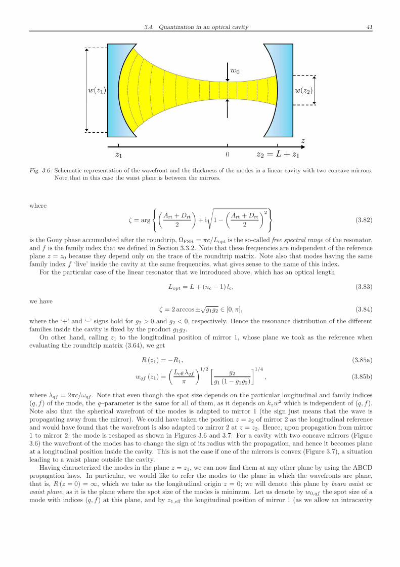
3.4. Quantization in an optical cavity 41

Fig. 3.6: Schematic representation of the wavefront and the thickness of the modes in a linear cavity with two concave mirrors.Note that in this case the waist plane is between the mirrors.

where

ζ = arg

(

Art +Drt

2

)

+ i

√

1−(

Art +Drt

2

)2

(3.82)

is the Gouy phase accumulated after the roundtrip, ΩFSR = πc/Lopt is the so-called free spectral range of the resonator,and f is the family index that we defined in Section 3.3.2. Note that these frequencies are independent of the referenceplane z = z0 because they depend only on the trace of the roundtrip matrix. Note also that modes having the samefamily index f ‘live’ inside the cavity at the same frequencies, what gives sense to the name of this index.

For the particular case of the linear resonator that we introduced above, which has an optical length

Lopt = L+ (nc − 1) lc, (3.83)

we haveζ = 2 arccos±√g1g2 ∈ [0, π], (3.84)

where the ‘+’ and ‘–’ signs hold for g2 > 0 and g2 < 0, respectively. Hence the resonance distribution of the differentfamilies inside the cavity is fixed by the product g1g2.

On other hand, calling z1 to the longitudinal position of mirror 1, whose plane we took as the reference whenevaluating the roundtrip matrix (3.64), we get

R (z1) = −R1, (3.85a)

wqf (z1) =

(

Leffλqfπ

)1/2 [g2

g1 (1− g1g2)

]1/4

, (3.85b)

where λqf = 2πc/ωqf . Note that even though the spot size depends on the particular longitudinal and family indices(q, f) of the mode, the q–parameter is the same for all of them, as it depends on kzw

2 which is independent of (q, f).Note also that the spherical wavefront of the modes is adapted to mirror 1 (the sign just means that the wave ispropagating away from the mirror). We could have taken the position z = z2 of mirror 2 as the longitudinal referenceand would have found that the wavefront is also adapted to mirror 2 at z = z2. Hence, upon propagation from mirror1 to mirror 2, the mode is reshaped as shown in Figures 3.6 and 3.7. For a cavity with two concave mirrors (Figure3.6) the wavefront of the modes has to change the sign of its radius with the propagation, and hence it becomes planeat a longitudinal position inside the cavity. This is not the case if one of the mirrors is convex (Figure 3.7), a situationleading to a waist plane outside the cavity.

Having characterized the modes in the plane z = z1, we can now find them at any other plane by using the ABCDpropagation laws. In particular, we would like to refer the modes to the plane in which the wavefronts are plane,that is, R (z = 0) = ∞, which we take as the longitudinal origin z = 0; we will denote this plane by beam waist orwaist plane, as it is the plane where the spot size of the modes is minimum. Let us denote by w0,qf the spot size of amode with indices (q, f) at this plane, and by z1,eff the longitudinal position of mirror 1 (as we allow an intracavity

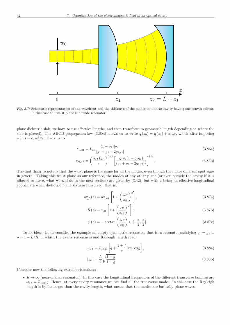
42 3. Quantization of the electromagnetic field in an optical cavity

Fig. 3.7: Schematic representation of the wavefront and the thickness of the modes in a linear cavity having one convex mirror.In this case the waist plane is outside resonator.

plane dielectric slab, we have to use effective lengths, and then transform to geometric length depending on where theslab is placed). The ABCD propagation law (3.60a) allows us to write q (z0) = q (z1) + z1,eff , which after imposingq (z0) = kzw

20/2i, leads us to

z1,eff = Leff(1− g1)|g2|

|g1 + g2 − 2g1g2|, (3.86a)

w0,qf =

(

λqfLeff

π

)1/2 [g1g2(1− g1g2)

(g1 + g2 − 2g1g2)2

]1/4

. (3.86b)

The first thing to note is that the waist plane is the same for all the modes, even though they have different spot sizesin general. Taking this waist plane as our reference, the modes at any other plane (or even outside the cavity if it isallowed to leave, what we will do in the next section) are given by (3.42), but with z being an effective longitudinalcoordinate when dielectric plane slabs are involved, that is,

w2qf (z) = w2

0,qf

[

1 +

(

zeffzR

)2]

, (3.87a)

R (z) = zeff

[

1 +

(

zRzeff

)2]

, (3.87b)

ψ (z) = − arctan

(

zeffzR

)

∈ [−π2,π

2]. (3.87c)

To fix ideas, let us consider the example an empty symmetric resonator, that is, a resonator satisfying g1 = g2 ≡g = 1− L/R, in which the cavity resonances and Rayleigh length read

ωqf = ΩFSR

[

q +1 + f

πarccos g

]

, (3.88a)

|zR| =L

2

√

1 + g

1− g . (3.88b)

Consider now the following extreme situations:

• R→∞ (near–planar resonator). In this case the longitudinal frequencies of the different transverse families areωqf = ΩFSRq. Hence, at every cavity resonance we can find all the transverse modes. In this case the Rayleighlength is by far larger than the cavity length, what means that the modes are basically plane waves.

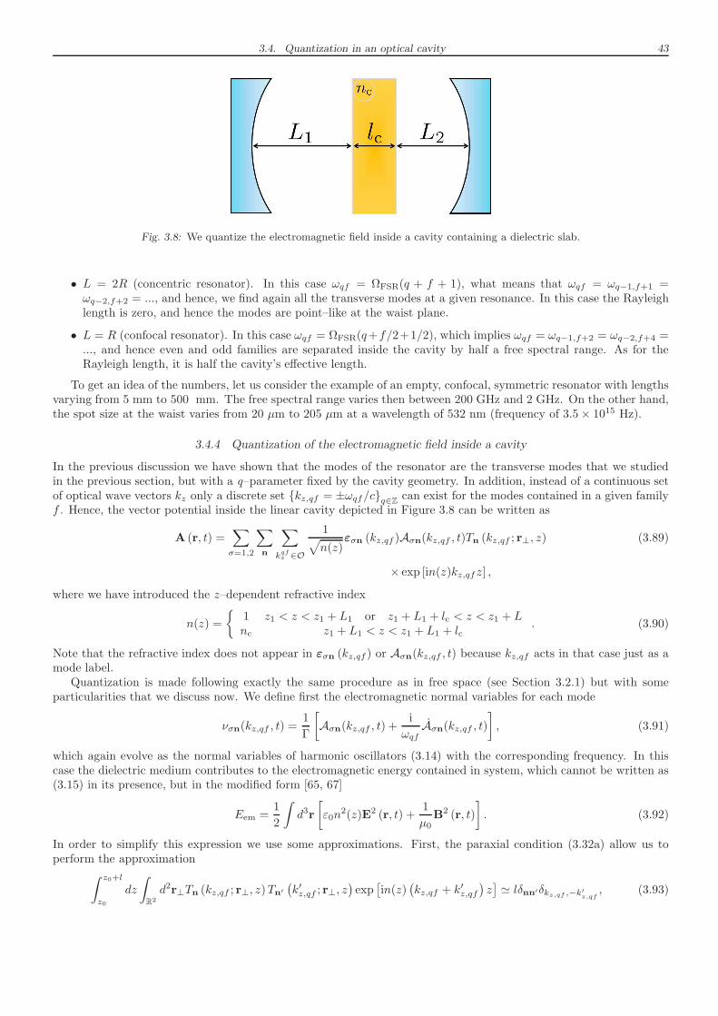
3.4. Quantization in an optical cavity 43

Fig. 3.8: We quantize the electromagnetic field inside a cavity containing a dielectric slab.

• L = 2R (concentric resonator). In this case ωqf = ΩFSR(q + f + 1), what means that ωqf = ωq−1,f+1 =ωq−2,f+2 = ..., and hence, we find again all the transverse modes at a given resonance. In this case the Rayleighlength is zero, and hence the modes are point–like at the waist plane.

• L = R (confocal resonator). In this case ωqf = ΩFSR(q+f/2+1/2), which implies ωqf = ωq−1,f+2 = ωq−2,f+4 =..., and hence even and odd families are separated inside the cavity by half a free spectral range. As for theRayleigh length, it is half the cavity’s effective length.

To get an idea of the numbers, let us consider the example of an empty, confocal, symmetric resonator with lengthsvarying from 5 mm to 500 mm. The free spectral range varies then between 200 GHz and 2 GHz. On the other hand,the spot size at the waist varies from 20 µm to 205 µm at a wavelength of 532 nm (frequency of 3.5× 1015 Hz).

3.4.4 Quantization of the electromagnetic field inside a cavity

In the previous discussion we have shown that the modes of the resonator are the transverse modes that we studiedin the previous section, but with a q–parameter fixed by the cavity geometry. In addition, instead of a continuous setof optical wave vectors kz only a discrete set kz,qf = ±ωqf/cq∈Z can exist for the modes contained in a given familyf . Hence, the vector potential inside the linear cavity depicted in Figure 3.8 can be written as

A (r, t) =∑

σ=1,2

∑

n

∑

kqfz ∈O

1√

n(z)εσn (kz,qf )Aσn(kz,qf , t)Tn (kz,qf ; r⊥, z) (3.89)

× exp [in(z)kz,qf z] ,

where we have introduced the z–dependent refractive index

n(z) =

1 z1 < z < z1 + L1 or z1 + L1 + lc < z < z1 + Lnc z1 + L1 < z < z1 + L1 + lc

. (3.90)

Note that the refractive index does not appear in εσn (kz,qf ) or Aσn(kz,qf , t) because kz,qf acts in that case just as amode label.

Quantization is made following exactly the same procedure as in free space (see Section 3.2.1) but with someparticularities that we discuss now. We define first the electromagnetic normal variables for each mode

νσn(kz,qf , t) =1

Γ

[

Aσn(kz,qf , t) +i

ωqfAσn(kz,qf , t)

]

, (3.91)

which again evolve as the normal variables of harmonic oscillators (3.14) with the corresponding frequency. In thiscase the dielectric medium contributes to the electromagnetic energy contained in system, which cannot be written as(3.15) in its presence, but in the modified form [65, 67]

Eem =1

2

∫

d3r

[

ε0n2(z)E2 (r, t) +

1

µ0B2 (r, t)

]

. (3.92)

In order to simplify this expression we use some approximations. First, the paraxial condition (3.32a) allow us toperform the approximation

∫ z0+l

z0

dz

∫

R2

d2r⊥Tn (kz,qf ; r⊥, z)Tn′

(

k′z,qf ; r⊥, z)

exp[

in(z)(

kz,qf + k′z,qf)

z]

≃ lδnn′δkz,qf ,−k′z,qf , (3.93)

44 3. Quantization of the electromagnetic field in an optical cavity

valid for any reference plane z = z0 as long as l ≫ |kz,qf |−1, |k′z,qf |−1, that is, as long as light is able to undergomany cycles between z = z0 and z = z0 + l. Then, the second paraxial condition (3.32b) leads to the approximation

∇ Tn (kz,qf ; r⊥, z) exp [in(z)kz,qfz] ≃ in(z)kz,qfezTn (kz,qf ; r⊥, z) exp [in(z)kz,qf z] . (3.94)

With this approximations at hand, it is straightforward to write the electromagnetic energy in terms of the normalvariables as

Eem =∑

σ=1,2

∑

n

∑

kqfz ∈O

ε0LoptΓ2ω2

qf

2ν∗σn(kz,qf )νσn(kz,qf ). (3.95)

The last particularity of optical cavities is that there is no sense in making a distinction between modes propagatingto the right or to the left, because they cannot be excited separately. Hence, we just define collective normal variablesνσqn = νσn(±|kz,qf |), so that the modes get completely specified inside the cavity by their polarization σ, and theirlongitudinal and transverse indices (q,n). Therefore, the electromagnetic energy can be finally written as

Eem =∑

σqn

ω2qf

2ν∗σqnνσqn, (3.96)

where we have chosen Γ = 1/√

2ε0Lopt so that this expression coincides with that of a collection of harmonic os-cillators as before. Quantization is therefore introduced by making a correspondence between the normal variablesνσqn(t), ν∗σqn(t) and boson operators

√

2~/ωqfaσqn(t), a†σqn(t) satisfying the commutation relations

[aσqn (t) , a†σ′q′n′ (t)] = δσσ′δqq′δnn′ , (3.97a)

[aσqn (t) , aσ′q′n′ (t)] = [a†σqn (t) , a†σ′q′n′ (t)] = 0. (3.97b)

The Hamiltonian of the electromagnetic field inside the cavity is then written as

Hem =∑

σqn

~ωqf a†σqnaσqn, (3.98)

where we have already removed the infinite contribution appearing when using the commutation relations to write itin normal order.

Finally, the vector potential inside the resonator is given by the operator

A(+) (r, t) =∑

σqn

1

2

√

~

n(z)ε0Loptωqfεσqnaσqn(t) Tn (kqf ; r⊥, z) exp [in(z)kqf z] + c.c. , (3.99)

where we have defined the positive definite modal wave vector kqf = ωqf/c, while the electric and magnetic fieldscorrespond then to

E(+) (r, t) = i∑

σqn

1

2

√

~ωqfn(z)ε0Lopt

εσqnaσqn(t) Tn (kqf ; r⊥, z) exp [in(z)kz,qf z] + c.c. , (3.100a)

B(+) (r, t) =i∑

σqn

1

2

√

n(z)~ωqfc2ε0Lopt

εσqnaσqn(t) Tn (kqf ; r⊥, z) exp [in(z)kz,qfz]− c.c. , (3.100b)

where the expressions emphasize the parts of the fields propagating to the right and to the left, which will be of laterconvenience even if their associated boson operators are the same.

4. QUANTUM THEORY OF OPEN CAVITIES

In the previous chapter we have been able to quantize the electromagnetic inside an optical cavity formed by perfectlyreflecting mirrors. However, in reality optical cavities must have at least one partially transmitting mirror allowingus to both inject light inside it and observe the intracavity processes by studying the light that comes out of it. Inthis section we explain how to deal with such an open cavity within the quantum formalism. To this aim we firstbuild a model for an open cavity with only one partially transmitting mirror, and then proceed to derive the evolutionequations satisfied by the intracavity field both in the Heisenberg and Schrodinger pictures.

In the last section, and as an example of another type of phenomenology that can be studied with the formalismof open quantum systems, we show how quantum–optical phenomena can be simulated with ultra–cold atoms trappedin optical lattices [68, 28] (a work developed by the author of the thesis at the Max–Planck Institute for QuantumOptics).

4.1 The open cavity model

For simplicity, we consider only one cavity mode with frequency ωc, polarization ε, and in the transverse modeT (ωc/c; r⊥, z), whose boson operators we denote by a, a†. The following discussion is straightforwardly generalizedto an arbitrary number of cavity modes.

We propose a model in which the cavity mode is coupled through the partially transmitting mirror to the externalmodes matching it in polarization and transverse shape. These external modes can be modeled as the modes of asecond cavity which shares the partially transmitting mirror with the real cavity, but has the second mirror placed atinfinity. According to the previous chapter, the field corresponding to such cavity can be written as

A (r, t) = limL→∞

∑

q

ε

2

√

~

ε0Lωqfbq(t) T (ωq/c; r⊥, z) exp [iωqz/c] + T (−ωq/c; r⊥, z) exp [−iωqz/c]+H.c., (4.1)

where the boson operators satisfy the commutation relations [bq(t), bq′ (t)] = δqq′ , and ωq = (πc/L)q + ∆ω⊥, being∆ω⊥ a contribution coming from the transverse structure of the modes, which is the same for all the longitudinalmodes. Now, as the length of this auxiliary cavity goes to infinity, the set of longitudinal modes becomes infinitelydense in frequency space, so that the sum over q can be replaced by the following integral:

limL→∞

∑

q

=L

πc

∫

O

dω. (4.2)

Accordingly, the Kronecker delta converges to a Dirac delta as

limL→∞

δqq′ =πc

Lδ(ω − ω′), (4.3)

so that defining new continuous boson operators by

b(ω) =

√

L

πclimL→∞

bq, (4.4)

which satisfy the commutation relations [b(ω), b†(ω′)] = δ(ω−ω′), we can finally write the vector potential of the fieldoutside the cavity as

A (r, t) =

∫

O

dω

√

~

4πcε0ωεb(ω; t) T (ω/c; r⊥, z) exp [iωz/c] + T (−ω/c; r⊥, z) exp [−iωz/c]+ H.c.. (4.5)

From the previous sections, we know that the free evolution of the cavity mode and the external modes is ruledby the Hamiltonian H0 = Hcav + Hext with

Hcav = ~ωca†a+ Hc and Hext =

∫

O

dω~ωb†(ω)b(ω), (4.6)

46 4. Quantum theory of open cavities

where Hc stands for any other intracavity process that we decide to introduce.The cavity and external modes are coupled through the mirror via a beam-splitter Hamiltonian

Hint = i~

∫

O

dωg(ω)[b†(ω)a− a†b(ω)], (4.7)

where the parameter g(ω) depends basically on the transmitivity of the mirror at the corresponding frequency, andsatisfies g2(ω)≪ ωc for optical frequencies. On the other hand, it is to be expected that only frequencies around thecavity frequency will contribute to the interaction (resonant interaction), what allows us to rewrite g(ω) =

√

γ/π interms of a frequency–independent constant γ, as the transmitivity of mirrors is a slowly varying function of frequencyat least within the interval [ωc − γ, ωc + γ], as well as extend the integration limits to [−∞,+∞], so that finally

Hint = i~

√

γ

π

∫ +∞

−∞

dω[b†(ω)a− a†b(ω)]. (4.8)

This is the basic model that we will use to ‘open the cavity’. In the following we show how to deduce reducedevolution equations for the intracavity mode only both at the level of operators (Heisenberg picture) and states(Schrodinger picture).

4.2 Heisenberg picture approach: The quantum Langevin equation

The Heisenberg equations of motion of the annihilation operators are

da

dt= −iωca+

[

a,Hc

i~

]

−√

γ

π

∫ +∞

−∞

dωb(ω), (4.9a)

db(ω)

dt= −iωb(ω) +

√

γ

πa. (4.9b)

We can formally integrate the second equation as

b(ω; t) = b0(ω)e−iωt +

√

γ

π

∫ t

0

dt′eiω(t′−t)a(t′), (4.10)

where b0(ω) are the external annihilation operators at the initial time. Introducing this solution into the evolutionequation for a, using

∫ τ1τ0dτf(τ)δ(τ − τ1) = f(τ1)/2, and defining the input operator

bin(t) = −1√2π

∫ +∞

−∞

dωe−iωtb0(ω), (4.11)

which is easily shown to satisfy the commutation relations

[bin(t), b†in(t′)] = δ(t− t′), (4.12a)

[bin(t), bin(t′)] = [b†in(t), b

†in(t′)] = 0, (4.12b)

we get

da

dt= −(γ + iωc)a+

[

a,Hc

i~

]

+√

2γbin(t), (4.13)

as the evolution equation for the intracavity mode.This equation is known as the quantum Langevin equation for its similarity with the stochastic Langevin equation,

the operator bin(t) playing the role of the stochastic noise. bin(t) is interpreted as the operator accounting for theinput field driving the cavity at each instant (see Figure 4.1). Indeed, note that when the external modes are in thevacuum state initially, we have

〈bin(t)〉 = 〈b†in(t)bin(t′)〉 = 0 and 〈bin(t)b†in(t′)〉 = δ(t− t′), (4.14)

so much like complex, Gaussian noises in stochastic Langevin equations.

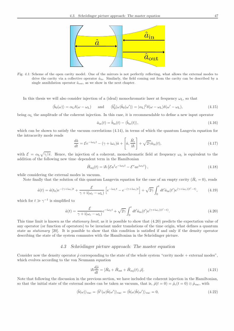
4.3. Schrodinger picture approach: The master equation 47

Fig. 4.1: Scheme of the open cavity model. One of the mirrors is not perfectly reflecting, what allows the external modes todrive the cavity via a collective operator ain. Similarly, the field coming out from the cavity can be described by asingle annihilation operator aout, as we show in the next chapter.

In this thesis we will also consider injection of a (ideal) monochromatic laser at frequency ωL, so that

〈b0(ω)〉 = αLδ(ω − ωL) and 〈b†0(ω)b0(ω′)〉 = |αL|2δ(ω − ωL)δ(ω′ − ωL), (4.15)

being αL the amplitude of the coherent injection. In this case, it is recommendable to define a new input operator

ain(t) = bin(t)− 〈bin(t)〉, (4.16)

which can be shown to satisfy the vacuum correlations (4.14), in terms of which the quantum Langevin equation forthe intracavity mode reads

da

dt= Ee−iωLt − (γ + iωc)a+

[

a,Hc

i~

]

+√

2γain(t), (4.17)

with E = αL

√

γ/π. Hence, the injection of a coherent, monochromatic field at frequency ωL is equivalent to theaddition of the following new time–dependent term in the Hamiltonian

Hinj(t) = i~(

Ea†e−iωLt − E∗aeiωLt)

, (4.18)

while considering the external modes in vacuum.Note finally that the solution of this quantum Langevin equation for the case of an empty cavity (Hc = 0), reads

a(t) = a(t0)e−(γ+iωc)t +

Eγ + i(ωc − ωL)

[

e−iωLt − e−(γ+iωc)t]

+√

2γ

∫ t

0

dt′ain(t′)e(γ+iωc)(t

′−t), (4.19)

which for t≫ γ−1 is simplified to

a(t) =E

γ + i(ωc − ωL)e−iωLt +

√

2γ

∫ t

0

dt′ain(t′)e(γ+iωc)(t

′−t). (4.20)

This time limit is known as the stationary limit, as it is possible to show that (4.20) predicts the expectation value ofany operator (or function of operators) to be invariant under translations of the time origin, what defines a quantumstate as stationary [20]. It is possible to show that this condition is satisfied if and only if the density operatordescribing the state of the system commutes with the Hamiltonian in the Schrodinger picture.

4.3 Schrodinger picture approach: The master equation

Consider now the density operator ρ corresponding to the state of the whole system “cavity mode + external modes”,which evolves according to the von Neumann equation

i~dρ

dt= [H0 + Hint + Hinj(t), ρ]. (4.21)

Note that following the discussion in the previous section, we have included the coherent injection in the Hamiltonian,so that the initial state of the external modes can be taken as vacuum, that is, ρ(t = 0) = ρc(t = 0)⊗ ρvac, with

〈b(ω)〉vac = 〈b†(ω)b(ω′)〉vac = 〈b(ω)b(ω′)〉vac = 0, (4.22)

48 4. Quantum theory of open cavities

where it is worth reminding that the expectation value of any external operator Aext is evaluated as 〈Aext〉vac =trextρvacAext.

We are going to work in the interaction picture (see Section A.3.2) defined by the transformation operator UI =U1U2, which is a sequence of two transformations defined as Uj = exp[Hjt/i~] with

H1 = ~ωL

[

a†a+

∫ +∞

−∞

dωb†(ω)b(ω)

]

, (4.23)

and

H2 = U †1

[

H0 + Hinj(t)]

U1 − H1 = ~∆ca†a+ Hc +

∫ +∞

−∞

dω~∆(ω)b†(ω)b(ω) + i~(

Ea† − E∗a)

. (4.24)

In this expression ∆c = ωc − ωL, ∆(ω) = ω − ωL, and we have assumed that [Hc, U1] = 0 (physically, this means thatwe consider only intracavity processes that conserve the number of photons). The first transformation rotates themodes to the laser frequency, and is performed in order to eliminate the time dependence of the Hamiltonian (of Hinj

in particular). The second one is made in order to remove all the pieces but Hint from the Hamiltonian, as a crucialincoming approximation requires the Hamiltonian to be ‘small’.

In this new picture, the state ρI = U †2 U†1 ρU1U2 evolves according to i~dρI/dt = [HI, ρI], with HI = U †2 U

†1HintU1U2.

Let us define the interaction picture intracavity annihilation operator

aI(t) = U †2 U†1 aU1U2, (4.25)

so that taking into account thatU †2 U

†1 b(ω)U1U2 = e−iωtb(ω), (4.26)

the interaction picture Hamiltonian can be rewritten as

HI(t) = i~

√

γ

π

∫ +∞

−∞

dω[

aI(t)b†(ω)eiωt − a†I (t)b(ω)e−iωt

]

. (4.27)

We seek now for the evolution equation of the reduced state ρCI = trextρI corresponding to the intracavity modealone. To do so, we first integrate formally the von Neumann equation for the whole system as

ρI(t) = ρI(t0) +1

i~

∫ t

0

dt′[HI(t′), ρI(t

′)]; (4.28)

reintroducing this expression into the von Neumann equation, making the partial trace over the external modes takinginto account that trext[HI(t), ρI(0)] ∼ 〈b〉vac = 0, and making the variable change t′ = t− τ in the time integral, weget the following integro–differential equation for the reduced density operator ρCI:

dρCI(t)

dt= − 1

~2

∫ t

0

dτtrext[HI(t), [HI(t− τ), ρI(t− τ)]]. (4.29)

This equation is exact, but now we are going to introduce two important approximations which lead to huge simpli-fications. The first is the Born approximation, which states that the external modes are basically unaffected by theintracavity dynamics, that is, ρI(t) = ρCI(t) ⊗ ρvac. Then we perform the Markov approximation, which states thatmemory effects can be neglected, that is, we can take ρI(t − τ) = ρI(t) in the integral kernel. It can be shown thatthis approximations are quite good in quantum optics thanks to the fact that γ/ωc ≪ 1 [69].

Introducing these approximations in (4.29), and performing the partial traces using (4.22), it is completely straight-forward to arrive to the following linear differential equation for the reduced intracavity state

dρCI

dt= 2γaIρCIa

†I − γa

†I aIρCI − γρCIa

†I aI, (4.30)

where all the operators are evaluated at the same time. Finally, coming back to the Schrodinger picture, we finallyarrive to

dρCdt

=

[

Hcav + Hinj(t)

i~, ρC

]

+ γ(

2aρCa† − a†aρC − ρCa†a

)

, (4.31)

where ρC = trextρ is the reduced state of the intracavity mode in the Schrodinger picture. This equation is knownas the master equation of the intracavity mode.

In order to evaluate intracavity moments of observables, in this thesis we will choose this Schrodinger approachin general. The reason is that having a master equation for the intracavity state only, we can apply the positive Ptechniques that we introduced at the end of Chapter 2 for the harmonic oscillator, what will allow us to deal withstochastic equations instead of operator equations of the type (4.17).

4.4. Relation of the model parameters to physical parameters 49

4.4 Relation of the model parameters to physical parameters

In the previous sections we have introduced the basic model that we will use for the evolution of a light mode insidean open cavity. The model turned out to have two basic parameters, E and γ, describing the rates at which coherentlight is injected into the cavity and intracavity light is lost through the partially transmitting mirror, respectively. Inthis section we connect these model parameters to relevant physical parameters like the transmitivity of the mirrorand the power of the injected laser beam.

This connection is easily done by following classical arguments. Consider the classical electromagnetic field asso-ciated to the intracavity mode, whose corresponding vector potential can be written as

A (r, t) =1

2

√

1

2n(z)ε0Loptεν(t)T (kc; r⊥, z) exp [in(z)kcz] + T ∗(kc; r⊥, z) exp [−in(z)kcz]+ c.c., (4.32)

in terms of the normal variable ν of the equivalent harmonic oscillator as we showed in Section 3.4.4. In this expressionwe have defined kc = ωc/c. Now, remember that in Chapter 2 we learned that the mean values of quantum observablesprovide the behavior of their classical counterparts as long as quantum fluctuations can be neglected (see also thediscussion at the beginning of Section 6.3.2). Applied to the cavity mode, this means that its classical normal variableevolves as ν(t) =

√

2~/ωc〈a(t)〉. Then, for an empty cavity (Hc = 0) and injecting on resonance for simplicity, thatis, ωL = ωc, we have

ν(t) = ν0e−(γ+iωc)t +

√

2~

ωc

Eγ

[

e−iωct − e−(γ+iωc)t]

, (4.33)

with ν0 = ν(t = 0), as follows from (4.19).Loss rate. We can connect the damping rate γ with the mirror transmitivity T (reflectivity R = 1−T ) by noting

that in the absence of injection, E = 0, a fraction R1/2 of the field amplitude is lost through the mirror at everyroundtrip; hence, after m ∈ N roundtrips, we will have the relation

A (r⊥, z ⊕m r.t., tm) = Rm/2A (r⊥, z, tm) , (4.34)

where ‘⊕mr.t.’ stands for ‘plus m–roundtrips’ and tm = 2mLopt/c. Introducing the solution (4.33) for ν(t) in thisexpression, and taking into account the definition of the cavity modes (3.78), it is straightforward to get

γ = − c

4LoptlnR ≃ cT

4Lopt, (4.35)

where in the last equality we have assumed that R ≈ 1. Hence, we see that for small mirror transmitivities, thereexists a linear relation between the model parameter γ and the actual mirror transmitivity T .

In order to understand the magnitude of this parameter let us consider a cavity with lengths varying between5 mm to 500 mm as in the previous chapter; the damping rate γ varies then between 150 MHz and 1.5 MHz forR = 0.99, and 1.5 GHz and 0.015 GHz for R = 0.9, which are well below optical frequencies. It is customary to callquality factor to the ratio between the free spectral range and the damping rate, Q = ΩFSR/γ. This parameter is veryimportant as it measures the ratio between the separation of the longitudinal resonances of a given transverse familyand the width of these. In other words, when the quality factor is large one can distinguish the different longitudinalresonances, while when it is small the Lorentzians associated to different resonances overlap, and the resonances areno longer distinguishable. In this thesis we will always work with cavities having large enough quality factors as canbe deduced from the numerical examples that we have introduced.

Injection parameter. Consider now the part of the intracavity vector potential propagating along the −ezdirection. According to (4.32) and (4.33), for a finite injection parameter E and in the stationary limit t ≫ γ−1, wecan write it as

A← (r, t) =1

2

√

~

n(z)ε0Loptωc

|E|γεT ∗(kc; r⊥, z)e

−in(z)kcz−iωct+iϕ + c.c., (4.36)

being ϕ the phase of the injected laser beam. On the other hand, based on (3.73) and (3.76), the vector potentialassociated to the laser inciding the cavity is written in terms of its power Pinj as

Ainj (r, t) =

√

Pinj

2ε0cω2c

εT ∗ (kc; r⊥, z) exp (−ikcz − iωct+ iϕ) + c.c., (4.37)

50 4. Quantum theory of open cavities

We can obtain an expression of the field inside the cavity by looking at it as an interferometer: The part of theinjection which is transmitted inside the cavity at a given time interferes with the fields that have been bouncing backand forth for several roundtrips. In this sense, the complete field will be a superposition of the fields

A(0) (r, t) = T 1/2Ainj (r, t) , (4.38a)

A(1) (r, t) = T 1/2R1/2Ainj (r⊥, z ⊕ r.t., t) , (4.38b)

A(2) (r, t) = T 1/2RAinj (r⊥, z ⊕2 r.t., t) , (4.38c)

...

A(m) (r, t) = T 1/2Rm/2Ainj (r⊥, z ⊕m r.t., t) , (4.38d)

and hence, assuming that the time is large enough as to take the m→∞ limit we get

A← (r, t) =

√

Pinj

2n(z)ε0cT 1/2

(

∞∑

m=0

Rm/2)

εT ∗ (kc; r⊥, z) e−ikcz−iωct+iϕ + c.c., (4.39)

where we have used again the definition of the cavity modes (3.78). Comparing (4.36) with this expression, andperforming the geometric sum we finally get

|E| = γ

√

2LPinj

~ωcc

T 1/2

1−R1/2≃√

2γ

~ωcPinj, (4.40)

where in the last equality we have assumed that R ≈ 1 and have made use of (4.35).

4.5 Quantum–optical phenomena with optical lattices

In connection with the theory of open quantum systems that we have particularized to optical cavities in this chapter,we now introduce the work that the author of this thesis started at the Max–Planck–Institute for Quantum Opticsduring a three–months visit in 2008, and that ended up published at the beginning of 2011 [28].

Ultracold atoms trapped in optical lattices are well known as quite versatile simulators of a large class of many–bodycondensed-matter Hamiltonians1 (see [72, 73, 74] for extensive reviews on this subject). In this work, and exploitingcurrently available technology only, we have been able to show that they can also be used to simulate phenomenatraditionally linked to quantum–optical systems, that is, to light–matter interactions [68, 28]. In this brief expositionof the work, we explain in particular how to observe phenomena arising from the collective spontaneous emissionof atomic and harmonic oscillator ensembles such as sub/superradiance, including some phenomena which still lackexperimental observation.

The concept of superradiance was introduced by Dicke in 1954 when studying the spontaneous emission of acollection of two–level atoms [78] (see [79] for a review). He showed that certain collective states where the excitationsare distributed symmetrically over the whole sample have enhanced emission rates. Probably the most stunningexample is the single–excitation symmetric state (now known as the symmetric Dicke state), which instead of decayingwith the single–atom decay rate Γ0, was shown to decay with NΓ0, N being the number of atoms. He also suggestedthat the emission rate of the state having all the atoms excited should be enhanced at the initial steps of the decayprocess, which was a most interesting prediction from the experimental point of view, as this state is in general easierto prepare. However, Dicke used a very simplified model in which all the atoms interact with a common radiationfield within the dipolar approximation; almost 15 years later, and motivated by the new atom–inversion techniques,several authors showed that dipolar interactions impose a threshold value for the atom density, that is, for the numberof interacting atoms, in order for superradiance to appear [80, 81, 82].

It is worth noting that together with atomic ensembles, spontaneous emission of collections of harmonic oscillatorswere also studied at that time [81]. Two interesting features of this system were reported: (i) an initial state with all

1 One of the first proposals in this direction was the article by Jacksch et al. [70], where it was proved that the dynamics of cold atomstrapped in optical lattices is described by the Bose–Hubbard Hamiltonian provided that certain conditions are satisfied; shortly after,the superfluid–to–Mott insulator phase transition characteristic of this Hamiltonian was observed in the laboratory [71]. Since then, thebroad tunability of the lattice parameters, and the increasing ability to trap different kind of particles (like bosonic and fermionic atomswith arbitrary spin or polar molecules), has allowed theoreticians to propose optical lattices as promising simulators for different types ofgeneralized Bose–Hubbard and spin models which are in close relation to important condensed–matter phenomena [72, 73, 74]. Recentexperiments have shown that optical lattices can be used to address open problems in physics like, e.g., high–Tc superconductivity [75],to study phenomena in low dimensions such as the Berezinskii–Kosterlitz–Thouless transition [76], or to implement quantum computationschemes [77].

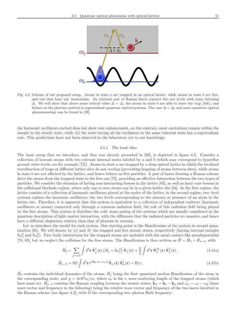
4.5. Quantum–optical phenomena with optical lattices 51

Fig. 4.2: Scheme of our proposed setup. Atoms in state a are trapped in an optical lattice, while atoms in state b are free,and can thus have any momentum. An external pair of Raman lasers connect the two levels with some detuning∆. We will show that above some critical value ∆ = ∆c the atoms in state b are able to leave the trap (left), andbehave as the photons emitted in superradiant quantum–optical systems. The case ∆ < ∆c and more quantum–opticalphenomenology can be found in [28].

the harmonic oscillators excited does not show rate enhancement, on the contrary, most excitations remain within thesample in the steady state, while (ii) the state having all the oscillators in the same coherent state has a superradiantrate. This predictions have not been observed in the laboratory yet to our knowledge.

4.5.1 The basic idea

The basic setup that we introduce, and that was already presented in [68], is depicted in figure 4.2. Consider acollection of bosonic atoms with two relevant internal states labeled by a and b (which may correspond to hyperfineground–state levels, see for example [72]). Atoms in state a are trapped by a deep optical lattice in which the localizedwavefunction of traps at different lattice sites do not overlap (preventing hopping of atoms between sites), while atomsin state b are not affected by the lattice, and hence behave as free particles. A pair of lasers forming a Raman schemedrive the atoms from the trapped state to the free one [72], providing an effective interaction between the two types ofparticles. We consider the situation of having non-interacting bosons in the lattice [83], as well as hard–core bosons inthe collisional blockade regime, where only one or zero atoms can be in a given lattice site [84]. In the first regime, thelattice consists of a collection of harmonic oscillators placed at the nodes of the lattice; in the second regime, two–levelsystems replace the harmonic oscillators, the two levels corresponding to the absence or presence of an atom in thelattice site. Therefore, it is apparent that this system is equivalent to a collection of independent emitters (harmonicoscillators or atoms) connected only through a common radiation field, the role of this radiation field being playedby the free atoms. This system is therefore the cold–atom analog of the systems which are usually considered in thequantum description of light–matter interaction, with the difference that the radiated particles are massive, and hencehave a different dispersion relation than that of photons in vacuum.

Let us introduce the model for such system. Our starting point is the Hamiltonian of the system in second quan-tization [85]. We will denote by |a〉 and |b〉 the trapped and free atomic states, respectively (having internal energies~ω0

a and ~ω0b ). Two–body interactions for the trapped atoms are included with the usual contact-like pseudopotential

[74, 83], but we neglect the collisions for the free atoms. The Hamiltonian is then written as H = H0 + Ha−b, with

H0 =∑

j=a,b

∫

d3r Ψ†j (r)(

Hj + ~ω0j

)

Ψj (r) +g

2

∫

d3r Ψ†2a (r) Ψ2a (r) , (4.41a)

Ha−b = ~Ω

∫

d3r ei(kL·r−ωLt)Ψa (r) Ψ†b (r) + H.c.; (4.41b)

H0 contains the individual dynamics of the atoms, Hj being the first–quantized motion Hamiltonian of the atom inthe corresponding state, and g = 4π~2as/m, where as is the s–wave scattering length of the trapped atoms (whichhave mass m). Ha−b contains the Raman coupling between the atomic states, kL = k1 − k2 and ωL = ω1 − ω2 (laserwave vector and frequency in the following) being the relative wave vector and frequency of the two lasers involved inthe Raman scheme (see figure 4.2), with Ω the corresponding two–photon Rabi frequency.

52 4. Quantum theory of open cavities

For atoms in state |a〉, Ha = −(

~2/2m

)

∇2 + Vopt (r), where Vopt (r) corresponds to a 3–dimensional opticallattice with cubic geometry and lattice period d0. We work with ultracold atoms under conditions such that theirwavefunctions can be described by the set of first–band Wannier functions localized around the nodes of the lattice[72]. The traps of the optical lattice are approximated by isotropic harmonic potentials [72], what allows us to writethe Wannier functions as

w0 (r− rj) =1

π3/4X3/20

exp[

− (r− rj)2/2X2

0

]

, (4.42)

where rj = d0j is the position of the j ∈ Z3 lattice site (we consider M sites in each orthogonal direction defining thecubic lattice), and X2

0 = ~/mω0, being ω0 the frequency of the harmonic trap. The energy associated to these wavefunctions is E0 = 3~ω0/2. We will assume that Wannier functions localized at different lattice sites do not overlap,hence preventing tunneling between sites.

On the other hand, atoms in state |b〉 can move freely in every direction of space according to Hb = −(

~2/2m)

∇2,

and hence the plane waves ψk (r) = eik·r/√V , with energy Ek = ~2k2/2m, are their motion eigenfunctions (V is the

total available volume for the free atoms, which we might take as infinite for calculations).We consider two opposite regimes for the interaction between trapped atoms. The first limit consists in neglecting

the interactions, which might be accomplished by, e.g., tuning the scattering length with an additional magnetic fieldthrough a Feshbach resonance [83]. Let us expand the quantum fields as

Ψa (r) =∑

j

w0 (r− rj) aj and Ψb (r) =∑

k

ψk (r) bk, (4.43)

where the operators aj, a†j and bk, b†k satisfy canonical bosonic commutation relations, and create or annihilate an

atom at lattice site j and a free atom with momentum k, respectively. Working in the interaction picture defined bythe transformation operator UI = exp[H0t/i~], we get the Hamiltonian

HI =∑

j,k

gk exp[i∆kt− i (k− kL) · rj]ajb†k +H.c., (4.44)

with

gk = ~Ω

√

8π3/2X30

Vexp

[

−1

2X2

0 (k− kL)2

]

, ∆k =~k2

2m−∆, (4.45)

∆ = ωL − (ωb − ωa) being the detuning of the laser frequency respect to the |a〉 |b〉 transition (ωa = ω0a + 3ω0/2

and ωb = ω0b ).

As for the second limit, we assume that the on–site repulsive atom–atom interaction is the dominant energy scale,and hence the trapped atoms behave as hard–core bosons in the collisional blockade regime, what prevents the presenceof two atoms in the same lattice site [84]; this means that the spectrum of a†j aj can be restricted to the first two states

|0〉j , |1〉j

, having 0 or 1 atoms at site j, and then the boson operators

a†j , aj

can be changed by spin-like ladder

operators

σ†j , σj

= |1〉j〈0|, |0〉j〈1|. In this second limit the Hamiltonian reads

HI =∑

j,k

gkei∆kt−i(k−kL)·rj σjb

†k +H.c.. (4.46)

Hamiltonians (4.44) and (4.46) show explicitly how this system mimics the dynamics of collections of harmonicoscillators or atoms, respectively, interacting with a common radiation field. Note finally that in order to satisfy thatthe trapped atoms are within the first Bloch band, it is required that ω0 ≫ ∆,Ω.

We are going to analyze the system by considering the free atoms as an environment for the trapped atoms, similarlyto the optical cavity, in which the external modes act as an environment for the intracavity modes. Following the sameapproach as that of Section 4.3, that is, assuming that the environment is in a non-evolving vacuum (Born–Markovapproximation) and tracing out its associated Hilbert space, it is simple [28] to get the following master equation forthe reduced density operator of the trapped atoms

dρ

dt=∑

j,l

Γj−lalρa†j − Γj−la

†j alρ+H.c.; (4.47)

a similar equation is obtained for the hard–core bosons but replacing the boson operators by the corresponding spinoperators. Note the similarity between this equation, and the equation of the damped mode inside the cavity (4.30),

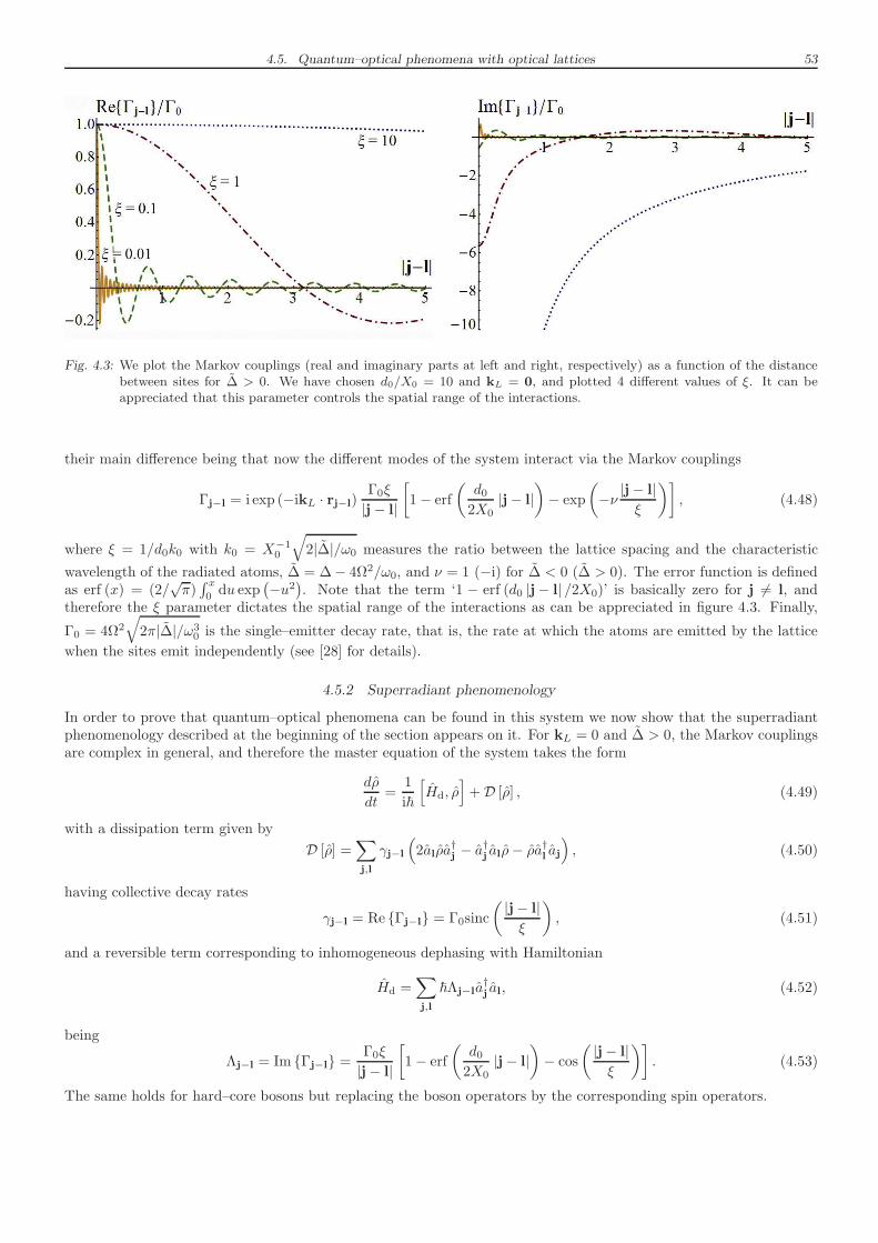
4.5. Quantum–optical phenomena with optical lattices 53

Fig. 4.3: We plot the Markov couplings (real and imaginary parts at left and right, respectively) as a function of the distancebetween sites for ∆ > 0. We have chosen d0/X0 = 10 and kL = 0, and plotted 4 different values of ξ. It can beappreciated that this parameter controls the spatial range of the interactions.

their main difference being that now the different modes of the system interact via the Markov couplings

Γj−l = i exp (−ikL · rj−l)Γ0ξ

|j− l|

[

1− erf

(

d02X0

|j− l|)

− exp

(

−ν |j− l|ξ

)]

, (4.48)

where ξ = 1/d0k0 with k0 = X−10

√

2|∆|/ω0 measures the ratio between the lattice spacing and the characteristic

wavelength of the radiated atoms, ∆ = ∆− 4Ω2/ω0, and ν = 1 (−i) for ∆ < 0 (∆ > 0). The error function is definedas erf (x) = (2/

√π)∫ x

0 du exp(

−u2)

. Note that the term ‘1 − erf (d0 |j− l| /2X0)’ is basically zero for j 6= l, andtherefore the ξ parameter dictates the spatial range of the interactions as can be appreciated in figure 4.3. Finally,

Γ0 = 4Ω2

√

2π|∆|/ω30 is the single–emitter decay rate, that is, the rate at which the atoms are emitted by the lattice

when the sites emit independently (see [28] for details).

4.5.2 Superradiant phenomenology

In order to prove that quantum–optical phenomena can be found in this system we now show that the superradiantphenomenology described at the beginning of the section appears on it. For kL = 0 and ∆ > 0, the Markov couplingsare complex in general, and therefore the master equation of the system takes the form

dρ

dt=

1

i~

[

Hd, ρ]

+D [ρ] , (4.49)

with a dissipation term given by

D [ρ] =∑

j,l

γj−l

(

2alρa†j − a

†j alρ− ρa

†l aj

)

, (4.50)

having collective decay rates

γj−l = Re Γj−l = Γ0sinc

( |j− l|ξ

)

, (4.51)

and a reversible term corresponding to inhomogeneous dephasing with Hamiltonian

Hd =∑

j,l

~Λj−la†j al, (4.52)

being

Λj−l = Im Γj−l =Γ0ξ

|j− l|

[

1− erf

(

d02X0

|j− l|)

− cos

( |j− l|ξ

)]

. (4.53)

The same holds for hard–core bosons but replacing the boson operators by the corresponding spin operators.

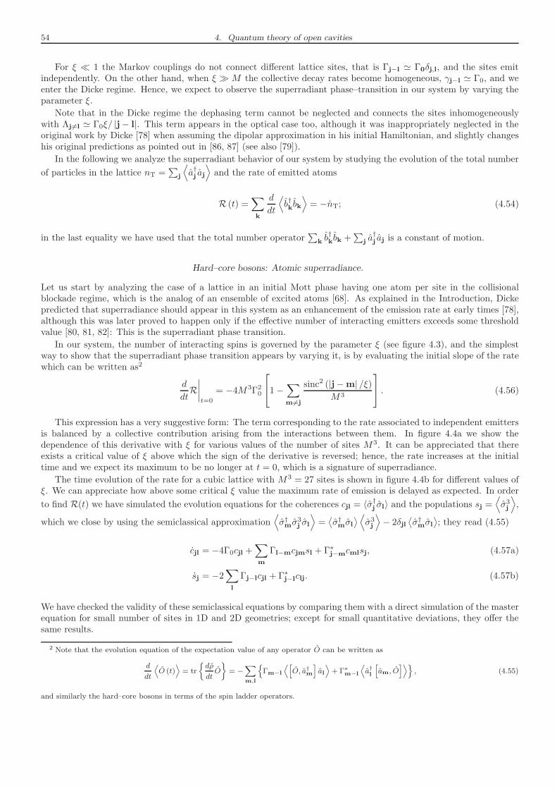
54 4. Quantum theory of open cavities

For ξ ≪ 1 the Markov couplings do not connect different lattice sites, that is Γj−l ≃ Γ0δj,l, and the sites emitindependently. On the other hand, when ξ ≫ M the collective decay rates become homogeneous, γj−l ≃ Γ0, and weenter the Dicke regime. Hence, we expect to observe the superradiant phase–transition in our system by varying theparameter ξ.

Note that in the Dicke regime the dephasing term cannot be neglected and connects the sites inhomogeneouslywith Λj6=l ≃ Γ0ξ/ |j− l|. This term appears in the optical case too, although it was inappropriately neglected in theoriginal work by Dicke [78] when assuming the dipolar approximation in his initial Hamiltonian, and slightly changeshis original predictions as pointed out in [86, 87] (see also [79]).

In the following we analyze the superradiant behavior of our system by studying the evolution of the total number

of particles in the lattice nT =∑

j

⟨

a†j aj

⟩

and the rate of emitted atoms

R (t) =∑

k

d

dt

⟨

b†kbk

⟩

= −nT; (4.54)

in the last equality we have used that the total number operator∑

k b†kbk +

∑

j a†j aj is a constant of motion.

Hard–core bosons: Atomic superradiance.

Let us start by analyzing the case of a lattice in an initial Mott phase having one atom per site in the collisionalblockade regime, which is the analog of an ensemble of excited atoms [68]. As explained in the Introduction, Dickepredicted that superradiance should appear in this system as an enhancement of the emission rate at early times [78],although this was later proved to happen only if the effective number of interacting emitters exceeds some thresholdvalue [80, 81, 82]: This is the superradiant phase transition.

In our system, the number of interacting spins is governed by the parameter ξ (see figure 4.3), and the simplestway to show that the superradiant phase transition appears by varying it, is by evaluating the initial slope of the ratewhich can be written as2

d

dtR∣

∣

∣

∣

t=0

= −4M3Γ20

1−∑

m6=j

sinc2 (|j−m| /ξ)M3

. (4.56)

This expression has a very suggestive form: The term corresponding to the rate associated to independent emittersis balanced by a collective contribution arising from the interactions between them. In figure 4.4a we show thedependence of this derivative with ξ for various values of the number of sites M3. It can be appreciated that thereexists a critical value of ξ above which the sign of the derivative is reversed; hence, the rate increases at the initialtime and we expect its maximum to be no longer at t = 0, which is a signature of superradiance.

The time evolution of the rate for a cubic lattice with M3 = 27 sites is shown in figure 4.4b for different values ofξ. We can appreciate how above some critical ξ value the maximum rate of emission is delayed as expected. In order

to find R(t) we have simulated the evolution equations for the coherences cjl = 〈σ†j σl〉 and the populations sj =⟨

σ3j

⟩

,

which we close by using the semiclassical approximation⟨

σ†mσ3j σl

⟩

=⟨

σ†mσl⟩

⟨

σ3j

⟩

− 2δjl⟨

σ†mσl⟩

; they read (4.55)

cjl = −4Γ0cjl +∑

m

Γl−mcjmsl + Γ∗j−mcmlsj, (4.57a)

sj = −2∑

l

Γj−lcjl + Γ∗j−lclj. (4.57b)

We have checked the validity of these semiclassical equations by comparing them with a direct simulation of the masterequation for small number of sites in 1D and 2D geometries; except for small quantitative deviations, they offer thesame results.

2 Note that the evolution equation of the expectation value of any operator O can be written as

d

dt

⟨

O (t)⟩

= tr

dρ

dtO

= −∑

m,l

Γm−l

⟨[

O, a†m

]

al

⟩

+ Γ∗m−l

⟨

a†l

[

am, O]⟩

, (4.55)

and similarly the hard–core bosons in terms of the spin ladder operators.

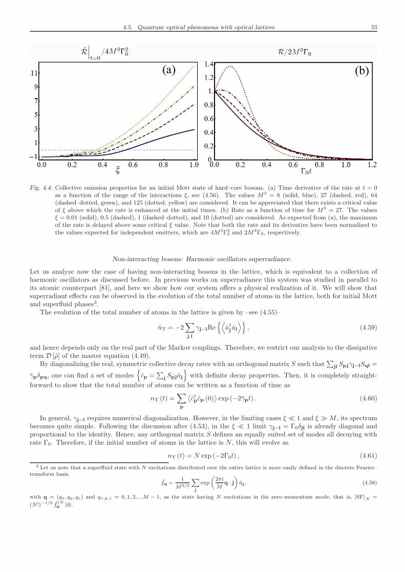
4.5. Quantum–optical phenomena with optical lattices 55

Fig. 4.4: Collective emission properties for an initial Mott state of hard–core bosons. (a) Time derivative of the rate at t = 0as a function of the range of the interactions ξ, see (4.56). The values M3 = 8 (solid, blue), 27 (dashed, red), 64(dashed–dotted, green), and 125 (dotted, yellow) are considered. It can be appreciated that there exists a critical valueof ξ above which the rate is enhanced at the initial times. (b) Rate as a function of time for M3 = 27. The valuesξ = 0.01 (solid), 0.5 (dashed), 1 (dashed–dotted), and 10 (dotted) are considered. As expected from (a), the maximumof the rate is delayed above some critical ξ value. Note that both the rate and its derivative have been normalized tothe values expected for independent emitters, which are 4M3Γ2

0 and 2M3Γ0, respectively.

Non-interacting bosons: Harmonic oscillators superradiance.

Let us analyze now the case of having non-interacting bosons in the lattice, which is equivalent to a collection ofharmonic oscillators as discussed before. In previous works on superradiance this system was studied in parallel toits atomic counterpart [81], and here we show how our system offers a physical realization of it. We will show thatsuperradiant effects can be observed in the evolution of the total number of atoms in the lattice, both for initial Mottand superfluid phases3.

The evolution of the total number of atoms in the lattice is given by –see (4.55)–

nT = −2∑

j,l

γj−lRe⟨

a†j al

⟩

, (4.59)

and hence depends only on the real part of the Markov couplings. Therefore, we restrict our analysis to the dissipativeterm D [ρ] of the master equation (4.49).

By diagonalizing the real, symmetric collective decay rates with an orthogonal matrix S such that∑

jl Spjγj−lSql =

γpδpq, one can find a set of modes

cp =∑

j Spjaj

with definite decay properties. Then, it is completely straight-

forward to show that the total number of atoms can be written as a function of time as

nT (t) =∑

p

⟨

c†pcp (0)⟩

exp (−2γpt) . (4.60)

In general, γj−l requires numerical diagonalization. However, in the limiting cases ξ ≪ 1 and ξ ≫M , its spectrumbecomes quite simple. Following the discussion after (4.53), in the ξ ≪ 1 limit γj−l = Γ0δjl is already diagonal andproportional to the identity. Hence, any orthogonal matrix S defines an equally suited set of modes all decaying withrate Γ0. Therefore, if the initial number of atoms in the lattice is N , this will evolve as

nT (t) = N exp (−2Γ0t) , (4.61)

3 Let us note that a superfluid state with N excitations distributed over the entire lattice is more easily defined in the discrete Fourier–transform basis

fq =1

M3/2

∑

j

exp

(2πi

Mq · j

)

aj, (4.58)

with q = (qx, qy, qz) and qx,y,z = 0, 1, 2, ...M − 1, as the state having N excitations in the zero–momentum mode, that is, |SF〉N =

(N !)−1/2 f†N0 |0〉.

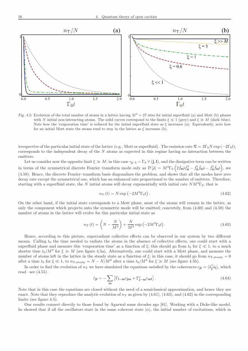
56 4. Quantum theory of open cavities

Fig. 4.5: Evolution of the total number of atoms in a lattice having M3 = 27 sites for initial superfluid (a) and Mott (b) phaseswith N initial non-interacting atoms. The solid curves correspond to the limits ξ ≪ 1 (grey) and ξ ≫M (dark–blue).Note how the ‘evaporation time’ is reduced for the initial superfluid state as ξ increases (a). Equivalently, note howfor an initial Mott state the atoms tend to stay in the lattice as ξ increases (b).

irrespective of the particular initial state of the lattice (e.g., Mott or superfluid). The emission rateR = 2Γ0N exp (−2Γ0t),corresponds to the independent decay of the N atoms as expected in this regime having no interaction between theemitters.

Let us consider now the opposite limit ξ ≫M ; in this case γj−l = Γ0 ∀ (j, l), and the dissipative term can be written

in terms of the symmetrical discrete Fourier–transform mode only as D [ρ] = M3Γ0

(

2f0ρf†0 − f †0 f0ρ− f †0f0ρ

)

, see

(4.58). Hence, the discrete Fourier–transform basis diagonalizes the problem, and shows that all the modes have zerodecay rate except the symmetrical one, which has an enhanced rate proportional to the number of emitters. Therefore,starting with a superfluid state, the N initial atoms will decay exponentially with initial rate NM3Γ0, that is

nT (t) = N exp(

−2M3Γ0t)

. (4.62)

On the other hand, if the initial state corresponds to a Mott phase, most of the atoms will remain in the lattice, asonly the component which projects onto the symmetric mode will be emitted; concretely, from (4.60) and (4.58) thenumber of atoms in the lattice will evolve for this particular initial state as

nT (t) =

(

N − N

M3

)

+N

M3exp

(

−2M3Γ0t)

. (4.63)

Hence, according to this picture, superradiant collective effects can be observed in our system by two differentmeans. Calling t0 the time needed to radiate the atoms in the absence of collective effects, one could start with asuperfluid phase and measure this ‘evaporation time’ as a function of ξ; this should go from t0 for ξ ≪ 1, to a muchshorter time t0/M

3 for ξ ≫ M (see figure 4.5a). Alternatively, one could start with a Mott phase, and measure thenumber of atoms left in the lattice in the steady state as a function of ξ; in this case, it should go from nT,steady = 0after a time t0 for ξ ≪ 1, to nT,steady = N −N/M3 after a time t0/M

3 for ξ ≫M (see figure 4.5b).

In order to find the evolution of nT we have simulated the equations satisfied by the coherences cjl = 〈a†j al〉, whichread –see (4.55)–

cjl = −∑

m

[

Γl−mcjm + Γ∗j−mcml

]

. (4.64)

Note that in this case the equations are closed without the need of a semiclassical approximation, and hence they areexact. Note that they reproduce the analytic evolution of nT as given by (4.61), (4.63), and (4.62) in the correspondinglimits (see figure 4.5).

Our results connect directly to those found by Agarwal some decades ago [81]. Working with a Dicke-like model,he showed that if all the oscillators start in the same coherent state |α〉, the initial number of excitations, which in

4.5. Quantum–optical phenomena with optical lattices 57

that case is given by N =M3 |α|2, decays following (4.62). This is not a coincidence, but rather a consequence that, ifN is large enough, a multi–coherent state of that kind is a good approximation of a superfluid state with that numberof excitations. He also predicted that if the oscillators start in a number state, most of the excitations would remainin the steady state as follows from (4.63).

58 4. Quantum theory of open cavities

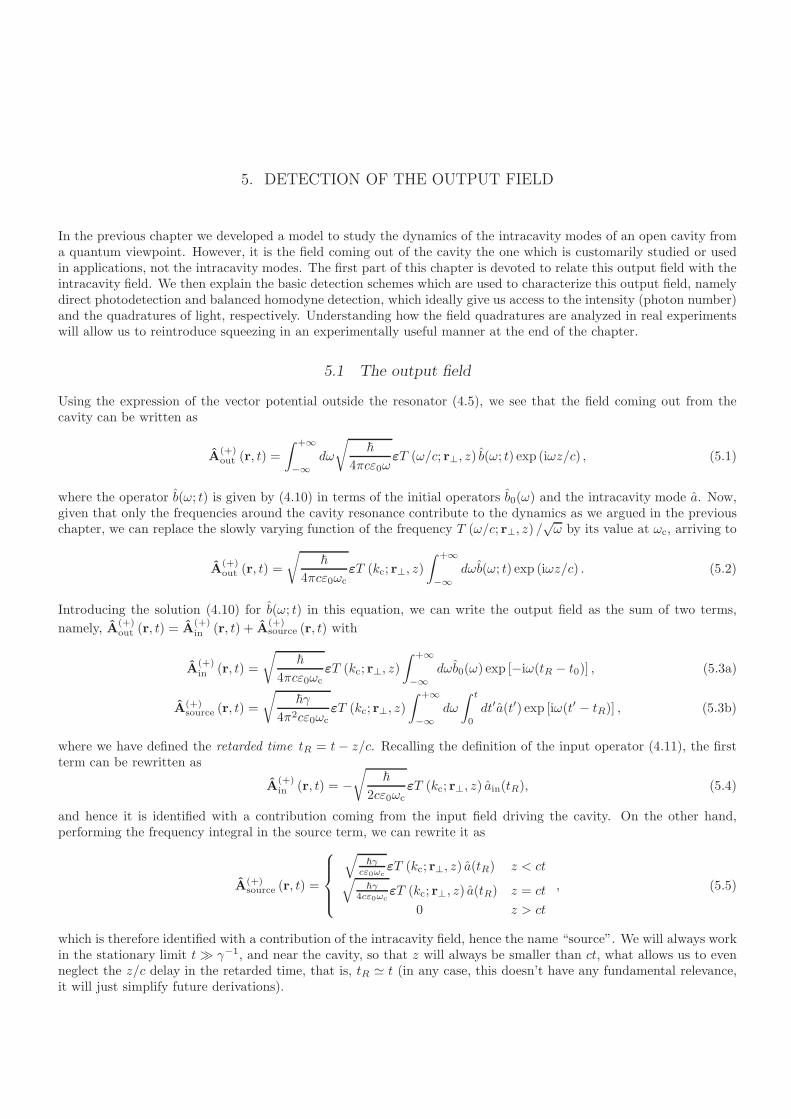
5. DETECTION OF THE OUTPUT FIELD

In the previous chapter we developed a model to study the dynamics of the intracavity modes of an open cavity froma quantum viewpoint. However, it is the field coming out of the cavity the one which is customarily studied or usedin applications, not the intracavity modes. The first part of this chapter is devoted to relate this output field with theintracavity field. We then explain the basic detection schemes which are used to characterize this output field, namelydirect photodetection and balanced homodyne detection, which ideally give us access to the intensity (photon number)and the quadratures of light, respectively. Understanding how the field quadratures are analyzed in real experimentswill allow us to reintroduce squeezing in an experimentally useful manner at the end of the chapter.

5.1 The output field

Using the expression of the vector potential outside the resonator (4.5), we see that the field coming out from thecavity can be written as

A(+)out (r, t) =

∫ +∞

−∞

dω

√

~

4πcε0ωεT (ω/c; r⊥, z) b(ω; t) exp (iωz/c) , (5.1)

where the operator b(ω; t) is given by (4.10) in terms of the initial operators b0(ω) and the intracavity mode a. Now,given that only the frequencies around the cavity resonance contribute to the dynamics as we argued in the previouschapter, we can replace the slowly varying function of the frequency T (ω/c; r⊥, z) /

√ω by its value at ωc, arriving to

A(+)out (r, t) =

√

~

4πcε0ωcεT (kc; r⊥, z)

∫ +∞

−∞

dωb(ω; t) exp (iωz/c) . (5.2)

Introducing the solution (4.10) for b(ω; t) in this equation, we can write the output field as the sum of two terms,

namely, A(+)out (r, t) = A

(+)in (r, t) + A

(+)source (r, t) with

A(+)in (r, t) =

√

~

4πcε0ωcεT (kc; r⊥, z)

∫ +∞

−∞

dωb0(ω) exp [−iω(tR − t0)] , (5.3a)

A(+)source (r, t) =

√

~γ

4π2cε0ωcεT (kc; r⊥, z)

∫ +∞

−∞

dω

∫ t

0

dt′a(t′) exp [iω(t′ − tR)] , (5.3b)

where we have defined the retarded time tR = t− z/c. Recalling the definition of the input operator (4.11), the firstterm can be rewritten as

A(+)in (r, t) = −

√

~

2cε0ωcεT (kc; r⊥, z) ain(tR), (5.4)

and hence it is identified with a contribution coming from the input field driving the cavity. On the other hand,performing the frequency integral in the source term, we can rewrite it as

A(+)source (r, t) =

√

~γcε0ωc

εT (kc; r⊥, z) a(tR) z < ct√

~γ4cε0ωc

εT (kc; r⊥, z) a(tR) z = ct

0 z > ct

, (5.5)

which is therefore identified with a contribution of the intracavity field, hence the name “source”. We will always workin the stationary limit t≫ γ−1, and near the cavity, so that z will always be smaller than ct, what allows us to evenneglect the z/c delay in the retarded time, that is, tR ≃ t (in any case, this doesn’t have any fundamental relevance,it will just simplify future derivations).

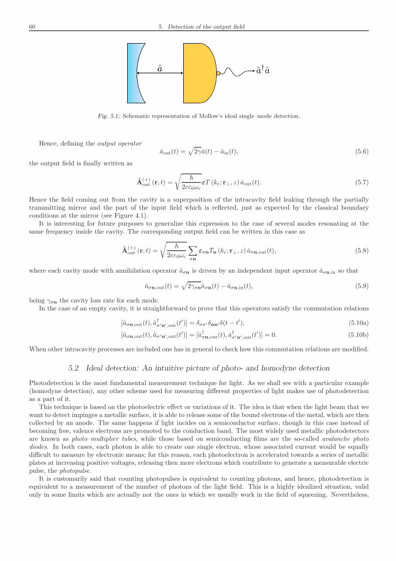
60 5. Detection of the output field

Fig. 5.1: Schematic representation of Mollow’s ideal single–mode detection.

Hence, defining the output operatoraout(t) =

√

2γa(t)− ain(t), (5.6)

the output field is finally written as

A(+)out (r, t) =

√

~

2cε0ωcεT (kc; r⊥, z) aout(t). (5.7)

Hence the field coming out from the cavity is a superposition of the intracavity field leaking through the partiallytransmitting mirror and the part of the input field which is reflected, just as expected by the classical boundaryconditions at the mirror (see Figure 4.1).

It is interesting for future purposes to generalize this expression to the case of several modes resonating at thesame frequency inside the cavity. The corresponding output field can be written in this case as

A(+)out (r, t) =

√

~

2cε0ωc

∑

σn

εσnTn (kc; r⊥, z) aσn,out(t), (5.8)

where each cavity mode with annihilation operator aσn is driven by an independent input operator aσn,in so that

aσn,out(t) =√

2γσnaσn(t)− aσn,in(t), (5.9)

being γσn the cavity loss rate for each mode.In the case of an empty cavity, it is straightforward to prove that this operators satisfy the commutation relations

[aσn,out(t), a†σ′n′,out(t

′)] = δσσ′δnn′δ(t− t′), (5.10a)

[aσn,out(t), aσ′n′,out(t′)] = [a†σn,out(t), a

†σ′n′,out(t

′)] = 0. (5.10b)

When other intracavity processes are included one has in general to check how this commutation relations are modified.

5.2 Ideal detection: An intuitive picture of photo- and homodyne detection

Photodetection is the most fundamental measurement technique for light. As we shall see with a particular example(homodyne detection), any other scheme used for measuring different properties of light makes use of photodetectionas a part of it.

This technique is based on the photoelectric effect or variations of it. The idea is that when the light beam that wewant to detect impinges a metallic surface, it is able to release some of the bound electrons of the metal, which are thencollected by an anode. The same happens if light incides on a semiconductor surface, though in this case instead ofbecoming free, valence electrons are promoted to the conduction band. The most widely used metallic photodetectorsare known as photo–multiplier tubes, while those based on semiconducting films are the so-called avalanche photodiodes. In both cases, each photon is able to create one single electron, whose associated current would be equallydifficult to measure by electronic means; for this reason, each photoelectron is accelerated towards a series of metallicplates at increasing positive voltages, releasing then more electrons which contribute to generate a measurable electricpulse, the photopulse.

It is customarily said that counting photopulses is equivalent to counting photons, and hence, photodetection isequivalent to a measurement of the number of photons of the light field. This is a highly idealized situation, validonly in some limits which are actually not the ones in which we usually work in the field of squeezing. Nevertheless,

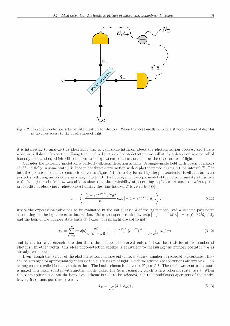
5.2. Ideal detection: An intuitive picture of photo- and homodyne detection 61

Fig. 5.2: Homodyne detection scheme with ideal photodetectors. When the local oscillator is in a strong coherent state, thissetup gives access to the quadratures of light.

it is interesting to analyze this ideal limit first to gain some intuition about the photodetection process, and this iswhat we will do in this section. Using this idealized picture of photodetectors, we will study a detection scheme calledhomodyne detection, which will be shown to be equivalent to a measurement of the quadratures of light.

Consider the following model for a perfectly efficient detection scheme. A single–mode field with boson operatorsa, a† initially in some state ρ is kept in continuous interaction with a photodetector during a time interval T . Theintuitive picture of such a scenario is shown in Figure 5.1: A cavity formed by the photodetector itself and an extraperfectly reflecting mirror contains a single mode. By developing a microscopic model of the detector and its interactionwith the light mode, Mollow was able to show that the probability of generating n photoelectrons (equivalently, theprobability of observing n photopulses) during the time interval T is given by [88]

pn =

⟨

:

(

1− e−κT)na†nan

n!exp

[

−(1− e−κT )a†a]

:

⟩

, (5.11)

where the expectation value has to be evaluated in the initial state ρ of the light mode, and κ is some parameteraccounting for the light–detector interaction. Using the operator identity :exp

[

−(1− e−λ)a†a]

: = exp(−λa†a) [15],and the help of the number state basis |n〉n∈N, it is straightforward to get

pn =

∞∑

m=n

〈n|ρ|n〉 m!

n!(m− n)!(

1− e−κT)n (

e−κT)m−n −→

T≫κ−1〈n|ρ|n〉, (5.12)

and hence, for large enough detection times the number of observed pulses follows the statistics of the number ofphotons. In other words, this ideal photodetection scheme is equivalent to measuring the number operator a†a asalready commented.

Even though the output of the photodetectors can take only integer values (number of recorded photopulses), theycan be arranged to approximately measure the quadratures of light, which we remind are continuous observables. Thisarrangement is called homodyne detection. The basic scheme is shown in Figure 5.2. The mode we want to measureis mixed in a beam splitter with another mode, called the local oscillator, which is in a coherent state |αLO〉. Whenthe beam splitter is 50/50 the homodyne scheme is said to be balanced, and the annihilation operators of the modesleaving its output ports are given by

a± =1√2(a± aLO) , (5.13)

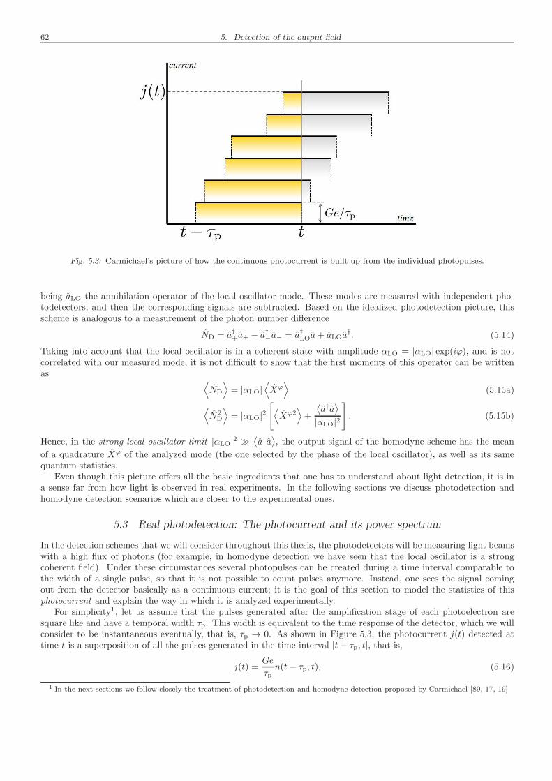
62 5. Detection of the output field

Fig. 5.3: Carmichael’s picture of how the continuous photocurrent is built up from the individual photopulses.

being aLO the annihilation operator of the local oscillator mode. These modes are measured with independent pho-todetectors, and then the corresponding signals are subtracted. Based on the idealized photodetection picture, thisscheme is analogous to a measurement of the photon number difference

ND = a†+a+ − a†−a− = a†LOa+ aLOa†. (5.14)

Taking into account that the local oscillator is in a coherent state with amplitude αLO = |αLO| exp(iϕ), and is notcorrelated with our measured mode, it is not difficult to show that the first moments of this operator can be writtenas

⟨

ND

⟩

= |αLO|⟨

Xϕ⟩

(5.15a)

⟨

N2D

⟩

= |αLO|2[

⟨

Xϕ2⟩

+

⟨

a†a⟩

|αLO|2

]

. (5.15b)

Hence, in the strong local oscillator limit |αLO|2 ≫⟨

a†a⟩

, the output signal of the homodyne scheme has the mean

of a quadrature Xϕ of the analyzed mode (the one selected by the phase of the local oscillator), as well as its samequantum statistics.

Even though this picture offers all the basic ingredients that one has to understand about light detection, it is ina sense far from how light is observed in real experiments. In the following sections we discuss photodetection andhomodyne detection scenarios which are closer to the experimental ones.

5.3 Real photodetection: The photocurrent and its power spectrum

In the detection schemes that we will consider throughout this thesis, the photodetectors will be measuring light beamswith a high flux of photons (for example, in homodyne detection we have seen that the local oscillator is a strongcoherent field). Under these circumstances several photopulses can be created during a time interval comparable tothe width of a single pulse, so that it is not possible to count pulses anymore. Instead, one sees the signal comingout from the detector basically as a continuous current; it is the goal of this section to model the statistics of thisphotocurrent and explain the way in which it is analyzed experimentally.

For simplicity1, let us assume that the pulses generated after the amplification stage of each photoelectron aresquare like and have a temporal width τp. This width is equivalent to the time response of the detector, which we willconsider to be instantaneous eventually, that is, τp → 0. As shown in Figure 5.3, the photocurrent j(t) detected attime t is a superposition of all the pulses generated in the time interval [t− τp, t], that is,

j(t) =Ge

τpn(t− τp, t), (5.16)

1 In the next sections we follow closely the treatment of photodetection and homodyne detection proposed by Carmichael [89, 17, 19]

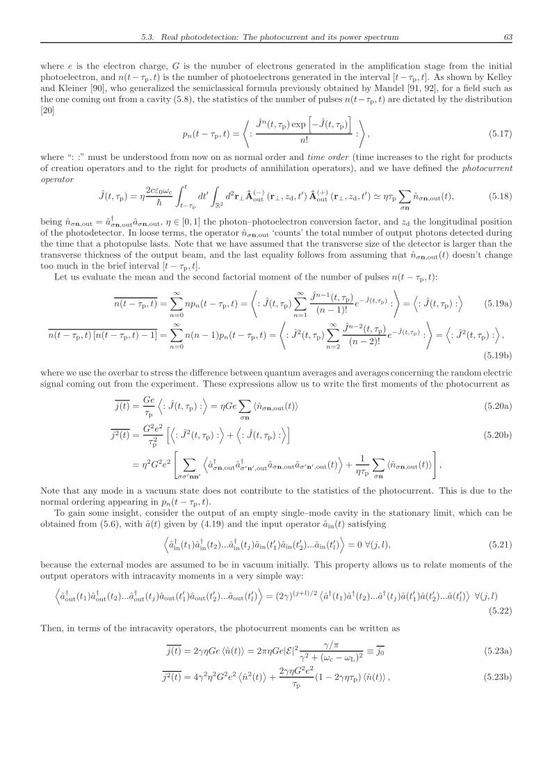
5.3. Real photodetection: The photocurrent and its power spectrum 63

where e is the electron charge, G is the number of electrons generated in the amplification stage from the initialphotoelectron, and n(t− τp, t) is the number of photoelectrons generated in the interval [t− τp, t]. As shown by Kelleyand Kleiner [90], who generalized the semiclassical formula previously obtained by Mandel [91, 92], for a field such asthe one coming out from a cavity (5.8), the statistics of the number of pulses n(t−τp, t) are dictated by the distribution[20]

pn(t− τp, t) =⟨

:Jn(t, τp) exp

[

−J(t, τp)]

n!:

⟩

, (5.17)

where “: :” must be understood from now on as normal order and time order (time increases to the right for productsof creation operators and to the right for products of annihilation operators), and we have defined the photocurrentoperator

J(t, τp) = η2cε0ωc

~

∫ t

t−τp

dt′∫

R2

d2r⊥A(−)out (r⊥, zd, t

′) A(+)out (r⊥, zd, t

′) ≃ ητp∑

σn

nσn,out(t), (5.18)

being nσn,out = a†σn,outaσn,out, η ∈ [0, 1] the photon–photoelectron conversion factor, and zd the longitudinal positionof the photodetector. In loose terms, the operator nσn,out ‘counts’ the total number of output photons detected duringthe time that a photopulse lasts. Note that we have assumed that the transverse size of the detector is larger than thetransverse thickness of the output beam, and the last equality follows from assuming that nσn,out(t) doesn’t changetoo much in the brief interval [t− τp, t].

Let us evaluate the mean and the second factorial moment of the number of pulses n(t− τp, t):

n(t− τp, t) =∞∑

n=0

npn(t− τp, t) =⟨

: J(t, τp)∞∑

n=1

Jn−1(t, τp)

(n− 1)!e−J(t,τp) :

⟩

=⟨

: J(t, τp) :⟩

(5.19a)

n(t− τp, t) [n(t− τp, t)− 1] =

∞∑

n=0

n(n− 1)pn(t− τp, t) =⟨

: J2(t, τp)

∞∑

n=2

Jn−2(t, τp)

(n− 2)!e−J(t,τp) :

⟩

=⟨

: J2(t, τp) :⟩

,

(5.19b)

where we use the overbar to stress the difference between quantum averages and averages concerning the random electricsignal coming out from the experiment. These expressions allow us to write the first moments of the photocurrent as

j(t) =Ge

τp

⟨

: J(t, τp) :⟩

= ηGe∑

σn

〈nσn,out(t)〉 (5.20a)

j2(t) =G2e2

τ2p

[⟨

: J2(t, τp) :⟩

+⟨

: J(t, τp) :⟩]

(5.20b)

= η2G2e2

[

∑

σσ′nn′

⟨

a†σn,outa†σ′n′,outaσn,outaσ′n′,out(t)

⟩

+1

ητp

∑

σn

〈nσn,out(t)〉]

,

Note that any mode in a vacuum state does not contribute to the statistics of the photocurrent. This is due to thenormal ordering appearing in pn(t− τp, t).

To gain some insight, consider the output of an empty single–mode cavity in the stationary limit, which can beobtained from (5.6), with a(t) given by (4.19) and the input operator ain(t) satisfying

⟨

a†in(t1)a†in(t2)...a

†in(tj)ain(t

′1)ain(t

′2)...ain(t

′l)⟩

= 0 ∀(j, l), (5.21)

because the external modes are assumed to be in vacuum initially. This property allows us to relate moments of theoutput operators with intracavity moments in a very simple way:⟨

a†out(t1)a†out(t2)...a

†out(tj)aout(t

′1)aout(t

′2)...aout(t

′l)⟩

= (2γ)(j+l)/2⟨

a†(t1)a†(t2)...a

†(tj)a(t′1)a(t

′2)...a(t

′l)⟩

∀(j, l)(5.22)

Then, in terms of the intracavity operators, the photocurrent moments can be written as

j(t) = 2γηGe 〈n(t)〉 = 2πηGe|E|2 γ/π

γ2 + (ωc − ωL)2≡ j0 (5.23a)

j2(t) = 4γ2η2G2e2⟨

n2(t)⟩

+2γηG2e2

τp(1 − 2γητp) 〈n(t)〉 , (5.23b)

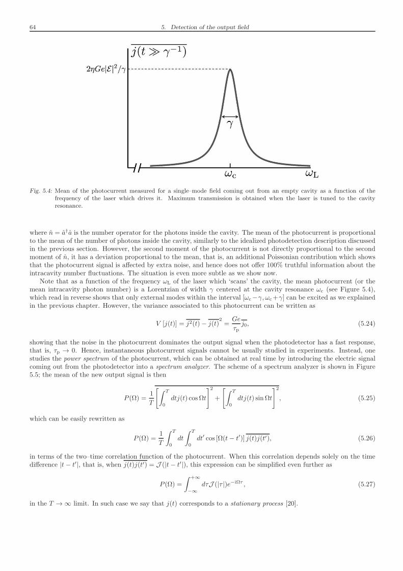
64 5. Detection of the output field

Fig. 5.4: Mean of the photocurrent measured for a single–mode field coming out from an empty cavity as a function of thefrequency of the laser which drives it. Maximum transmission is obtained when the laser is tuned to the cavityresonance.

where n = a†a is the number operator for the photons inside the cavity. The mean of the photocurrent is proportionalto the mean of the number of photons inside the cavity, similarly to the idealized photodetection description discussedin the previous section. However, the second moment of the photocurrent is not directly proportional to the secondmoment of n, it has a deviation proportional to the mean, that is, an additional Poissonian contribution which showsthat the photocurrent signal is affected by extra noise, and hence does not offer 100% truthful information about theintracavity number fluctuations. The situation is even more subtle as we show now.

Note that as a function of the frequency ωL of the laser which ‘scans’ the cavity, the mean photocurrent (or themean intracavity photon number) is a Lorentzian of width γ centered at the cavity resonance ωc (see Figure 5.4),which read in reverse shows that only external modes within the interval [ωc−γ, ωc+γ] can be excited as we explainedin the previous chapter. However, the variance associated to this photocurrent can be written as

V [j(t)] = j2(t)− j(t)2 =Ge

τpj0, (5.24)

showing that the noise in the photocurrent dominates the output signal when the photodetector has a fast response,that is, τp → 0. Hence, instantaneous photocurrent signals cannot be usually studied in experiments. Instead, onestudies the power spectrum of the photocurrent, which can be obtained at real time by introducing the electric signalcoming out from the photodetector into a spectrum analyzer. The scheme of a spectrum analyzer is shown in Figure5.5; the mean of the new output signal is then

P (Ω) =1

T

[

∫ T

0

dtj(t) cosΩt

]2

+

[

∫ T

0

dtj(t) sinΩt

]2

, (5.25)

which can be easily rewritten as

P (Ω) =1

T

∫ T

0

dt

∫ T

0

dt′ cos [Ω(t− t′)] j(t)j(t′), (5.26)

in terms of the two–time correlation function of the photocurrent. When this correlation depends solely on the timedifference |t− t′|, that is, when j(t)j(t′) = J (|t− t′|), this expression can be simplified even further as

P (Ω) =

∫ +∞

−∞

dτJ (|τ |)e−iΩτ , (5.27)

in the T →∞ limit. In such case we say that j(t) corresponds to a stationary process [20].

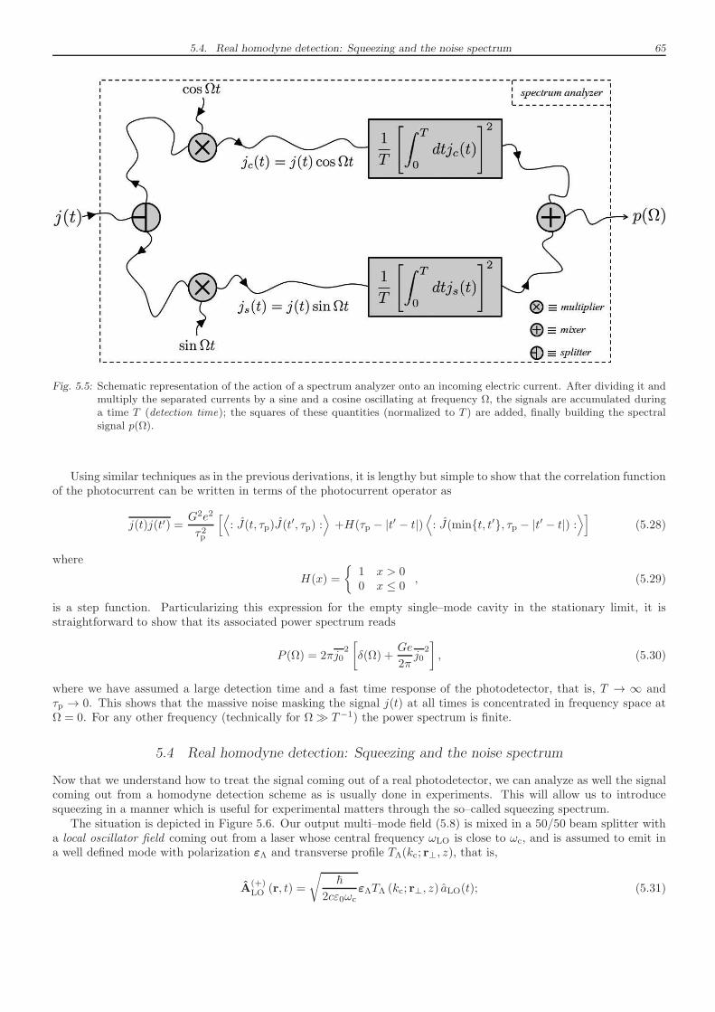
5.4. Real homodyne detection: Squeezing and the noise spectrum 65

Fig. 5.5: Schematic representation of the action of a spectrum analyzer onto an incoming electric current. After dividing it andmultiply the separated currents by a sine and a cosine oscillating at frequency Ω, the signals are accumulated duringa time T (detection time); the squares of these quantities (normalized to T ) are added, finally building the spectralsignal p(Ω).

Using similar techniques as in the previous derivations, it is lengthy but simple to show that the correlation functionof the photocurrent can be written in terms of the photocurrent operator as

j(t)j(t′) =G2e2

τ2p

[⟨

: J(t, τp)J(t′, τp) :

⟩

+H(τp − |t′ − t|)⟨

: J(mint, t′, τp − |t′ − t|) :⟩]

(5.28)

where

H(x) =

1 x > 00 x ≤ 0

, (5.29)

is a step function. Particularizing this expression for the empty single–mode cavity in the stationary limit, it isstraightforward to show that its associated power spectrum reads

P (Ω) = 2πj02[

δ(Ω) +Ge

2πj0

2]

, (5.30)

where we have assumed a large detection time and a fast time response of the photodetector, that is, T → ∞ andτp → 0. This shows that the massive noise masking the signal j(t) at all times is concentrated in frequency space atΩ = 0. For any other frequency (technically for Ω≫ T−1) the power spectrum is finite.

5.4 Real homodyne detection: Squeezing and the noise spectrum

Now that we understand how to treat the signal coming out of a real photodetector, we can analyze as well the signalcoming out from a homodyne detection scheme as is usually done in experiments. This will allow us to introducesqueezing in a manner which is useful for experimental matters through the so–called squeezing spectrum.

The situation is depicted in Figure 5.6. Our output multi–mode field (5.8) is mixed in a 50/50 beam splitter witha local oscillator field coming out from a laser whose central frequency ωLO is close to ωc, and is assumed to emit ina well defined mode with polarization εΛ and transverse profile TΛ(kc; r⊥, z), that is,

A(+)LO (r, t) =

√

~

2cε0ωcεΛTΛ (kc; r⊥, z) aLO(t); (5.31)

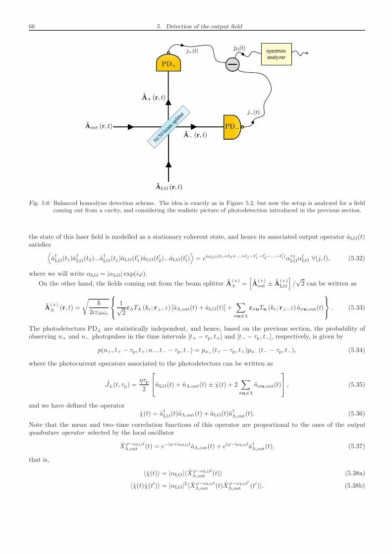
66 5. Detection of the output field

Fig. 5.6: Balanced homodyne detection scheme. The idea is exactly as in Figure 5.2, but now the setup is analyzed for a fieldcoming out from a cavity, and considering the realistic picture of photodetection introduced in the previous section.

the state of this laser field is modelled as a stationary coherent state, and hence its associated output operator aLO(t)satisfies

⟨

a†LO(t1)a†LO(t2)...a

†LO(tj)aLO(t

′1)aLO(t

′2)...aLO(t

′l)⟩

= eiωLO(t1+t2+...+tj−t′

1−t′

2−...−t′

l)α∗jLOαlLO ∀(j, l), (5.32)

where we will write αLO = |αLO| exp(iϕ).On the other hand, the fields coming out from the beam splitter A

(+)± =

[

A(+)out ± A

(+)LO

]

/√2 can be written as

A(+)± (r, t) =

√

~

2cε0ωc

1√2εΛTΛ (kc; r⊥, z) [aΛ,out(t) + aLO(t)] +

∑

σn 6=Λ

εσnTn (kc; r⊥, z) aσn,out(t)

. (5.33)

The photodetectors PD± are statistically independent, and hence, based on the previous section, the probability ofobserving n+ and n− photopulses in the time intervals [t+ − τp, t+] and [t− − τp, t−], respectively, is given by

p(n+, t+ − τp, t+;n−, t− − τp, t−) = pn+(t+ − τp, t+)pn−

(t− − τp, t−), (5.34)

where the photocurrent operators associated to the photodetectors can be written as

J±(t, τp) =ητp2

nLO(t) + nΛ,out(t)± χ(t) + 2∑

σn 6=Λ

nσn,out(t)

, (5.35)

and we have defined the operatorχ(t) = a†LO(t)aΛ,out(t) + aLO(t)a

†Λ,out(t). (5.36)

Note that the mean and two–time correlation functions of this operator are proportional to the ones of the outputquadrature operator selected by the local oscillator

Xϕ−ωLOtΛ,out (t) = e−iϕ+iωLOtaΛ,out(t) + eiϕ−iωLOta†Λ,out(t), (5.37)

that is,

〈χ(t)〉 = |αLO|〈Xϕ−ωLOtΛ,out (t)〉 (5.38a)

〈χ(t)χ(t′)〉 = |αLO|2〈Xϕ−ωLOtΛ,out (t)Xϕ−ωLOt

′

Λ,out (t′)〉. (5.38b)

5.4. Real homodyne detection: Squeezing and the noise spectrum 67

The fast optical oscillations of the aΛ,out(t) operator are canceled by the rapidly oscillating function exp(iωLOt) addedby the local oscillator. In order to simplify the derivations, it is then customary to move to an interaction picturedefined by the transformation operator U0 = exp[H0t/i~] with

H0 =∑

σn

~ωLO

[

a†σnaσn +

∫ +∞

−∞

dωb†σn(ω)bσn(ω)

]

, (5.39)

so thatU †0 X

ϕ−ωLOtΛ,out U0 = Xϕ

Λ,out, (5.40)

that is, the fast linear variation of the quadrature’s phase is removed. From now on, we assume to work in this picture,that is, quantum expectation values are to be taken with the interaction picture state ρI(t) = U †0 ρ(t)U0. We shall seehow useful this picture is in the next chapter, when analyzing the squeezing properties of optical parametric oscillators.

It is not difficult to prove that in the strong local oscillator regime, the difference photocurrent jD(t) = j+(t)−j−(t)carries information about the χ(t) operator only; any other possible contribution to this photocurrent is balanced outthanks to the 50/50 beam splitter. To this aim we evaluate the first moments of the difference photocurrent, which,given the statistical independency of the photodetectors, can be written in terms of the moments of j±(t) as

jD(t) = j+(t)− j−(t) and j2D(t) = j2+(t) + j2−(t)− 2j+(t)× j−(t). (5.41)

Making use of the relation (5.20) between the moments of j±(t) and the quantum expectation values of their corre-sponding photocurrent operators (5.35), it is straightforward to show after some algebra that the mean and varianceof the difference photocurrent are given by

jD(t) = ηGe|αLO|⟨

XϕΛ,out

⟩

, (5.42a)

V [jD(t)] =η2G2e2|αLO|2

τp

(

1 +∑

σn

〈nσn,out〉|αLO|2

)

+ η3G2e2|αLO|2[

⟨

:(

δXϕΛ,out

)2

:

⟩

+∑

σn

⟨

: δn2σn,out :

⟩

|αLO|2

]

, (5.42b)

where we remind that we make use of the notation δB = B − 〈B〉. Taking the strong local oscillator limit

|αLO|2 ≫

〈nσn,out〉 ,⟨

: δn2σn,out :

⟩

∀(σn), (5.43)

the variance of the difference photocurrent is written as

V [jD(t)] = η2G2e2|αLO|2

1

τp+ η〈: [δXϕ

Λ,out(t)]2 :〉

. (5.44)

Expression (5.42a) shows that the mean of jD(t) carries information about the quadrature of the mode selected bythe local oscillator, but similarly to the direct detection case, in the fast response limit τp → 0 this signal is maskedby massive noise at all times.

Hence, also in homodyne detection one is forced to consider the power spectrum of the difference photocurrent.As there are no contributions from any of the modes with (σ,n) 6= Λ, we will remove the local oscillator mode indexΛ from now on. Using again the statistical independency of the signals coming out from the photodetectors PD±, onecan write the two–time correlation function of jD(t) as

jD(t)jD(t′) = j+(t)j+(t′) + j−(t)j−(t′)− j+(t)× j−(t′)− j+(t′)× j−(t). (5.45)

Using now the general expression (5.28) for the two–time correlation function of a photocurrent, it is lengthy buttrivial to arrive to the following expression for the power spectrum of jD(t)

PD(Ω) =1

T

∫ T

0

dt

∫ T

0

dt′ cos [Ω(t− t′)] jD(t)jD(t′) = Pshot + P (Ω), (5.46)

beingPshot = ηG2e2|αLO|2, (5.47)

a contribution to the spectrum which does not depend either on the state of the system or in the frequency (theso-called shot noise contribution), and

P (Ω) =η2G2e2

T

∫ T

0

dt

∫ T

0

dt′ cos [Ω(t− t′)]⟨

: δXϕout(t)δX

ϕout(t

′) :⟩

(5.48)

68 5. Detection of the output field

a contribution which does depend on these.It is customary to define a normalized version of this quantity called the noise spectrum

V out(Xϕ; Ω) =PD(Ω)

Pshot= 1+ Sout(Xϕ; Ω) (5.49)

where

Sout(

Xϕ; Ω)

=η

T

∫ T

0

dt

∫ T

0

dt′ cos [Ω(t− t′)] 〈: δXϕout(t)δX

ϕout(t

′) :〉, (5.50)

is the so-called squeezing spectrum, which, when 〈: δXϕout(t)δX

ϕout(t

′) :〉 depends only on |t− t′|, that is, for stationarystates, can be written as

Sout(

Xϕ; Ω)

= η

∫ +∞

−∞

dt′〈: δXϕout(t)δX

ϕout(t+ t′) :〉e−iΩt′ . (5.51)

Accordingly, we will call noise frequency to Ω, which needs not to be confused with the optical frequencies.Note that the multi–time moments of the output operators still satisfy (5.22), and hence, in terms of the quadratures

of the intracavity mode the squeezing spectrum reads

Sout(Xϕ; Ω) =2γη

T

∫ T

0

dt

∫ T

0

dt′ cos [Ω(t− t′)] 〈: δXϕ(t)δXϕ(t′) :〉, (5.52)

and similarly for the stationary expression. Hence, knowing the state of the intracavity mode, we can evaluate thenoise spectrum measured for the field coming out from the cavity. In the upcoming chapters we will assume unitconversion efficiency2, that is, η = 1.

In Chapter 2 we introduced squeezed states of a single harmonic oscillator as those in which one of its quadratureshad an uncertainty below that of vacuum or a coherent state. However, we have seen that this simple intuitive object(the uncertainty of a single–mode quadrature) is not the relevant quantity in real experiments designed to measurethe quadratures of light, and hence we need to come back a little bit and redefine the concept of squeezing in a waywhich is interesting from the experimental point of view.

To this aim, let us proceed similarly to how we did in Chapter 2. Consider a quasiperiodic modulation of frequencyΩsignal encoded in some quadrature of a cavity mode. It is to be expected that such modulation will appear inthe noise spectrum of the corresponding output mode as a peak centered at the Ω = Ωsignal. The problem is thatif this modulation is very small, the corresponding peak in the spectrum can be disguised by the basal shot noisecontribution, and it will be impossible to observe it. This is indeed the case when the state of the light mode iscoherent (like vacuum), as then the squeezing spectrum is zero for any quadrature and at any noise frequency, so thatthe noise spectrum has only the flat V out(Xϕ; Ω) = 1 shot noise contribution. We can then define squeezed statesof light in an experimentally useful manner as those states in which V out(Xϕ; Ω) < 1 for some quadrature and somefrequency.

It is not difficult to show that the noise spectra associated to two orthogonal quadratures satisfy the Heisenberguncertainty relation

V out(Xϕ; Ω)V out(Xϕ+π/2; Ω) ≥ 1. (5.53)

Hence, if the shot noise contribution is balanced out for some quadrature, it will be increased accordingly for itsorthogonal quadrature, similarly to what happened with the uncertainty of single–mode quadratures in the discussionof Chapter 2.

2 Real experiments are not that far from this situation, arriving to efficiencies above 90%.

6. QUANTUM DESCRIPTION AND BASIC PROPERTIESOF OPTICAL PARAMETRIC OSCILLATORS

In the previous chapters we have developed the basic tools which allow us to study within the quantum formalism thelight generated in optical cavities. It is now time to apply these to a specific system, optical parametric oscillators,which will be shown to be ideal candidates for the generation of squeezed and entangled light.

Such systems belong to the class of so-called nonlinear optical cavities, that is, resonators containing a nonlinearoptical medium. For this reason, the first section of the chapter contains a brief introduction to the optics of dielectricmedia, with special emphasis on nonlinear uniaxial crystals and the three–wave mixing processes that occur insidethem. We then introduce the model for optical parametric oscillators that will be used all along this thesis, and studythe quantum properties of the light generated by them in different regimes.

6.1 Dielectric media and nonlinear optics

Roughly speaking [65, 67], from the point of view of their electromagnetic properties most materials fit either intothe class of conductors or the class of dielectrics. A conducting material has charges which are free to move throughit, and hence the application of an electromagnetic field can induce an electric current on it. On the other hand,in dielectric media every charge is strongly bounded to one specific atom or molecule fixed in some position of thematerial, and hence these can be seen as insulators. However, when an electromagnetic field is applied to a dielectric,the electron cloud surrounding each nucleus can be slightly displaced, what means that the center of mass of thepositive and negative charge distributions of the atoms or molecules get slightly separated, and then the mediumacquires a polarization, that is, a dipole moment per unit volume. In this section we briefly introduce the descriptionof the electromagnetic field in such media from a classical viewpoint. We will work only with dielectrics which aresensitive to the electric field, but not to the magnetic field.

In principle, in order to describe the effects appearing in the field when propagating in the dielectric materialone needs to develop a microscopic model for the medium, introduce it in the inhomogeneous Maxwell’s equationsvia a charge distribution ρ(r, t) and a current distribution j(r, t), and then solve the resulting field–medium coupledequations. However, for the type of media we will work with and for weak enough electromagnetic fields, one canassume that the polarization P (r, t) acquired by the medium is a low order polynomial of the applied electric field,say1

Pj (r, t) = ε0χ(1)jk Ek (r, t) + ε0χ

(2)jklEk (r, t)El (r, t) + ..., (6.1)

so that the medium can be treated as a non-dynamical system whose information is all contained the←→χ (n) coefficients(tensors of order n + 1 technically2), called the n–order susceptibilities. In such circumstances one can define adisplacement field

D (r, t) = ε0E (r, t) +P (r, t) , (6.2)

and replace the inhomogeneous Maxwell’s equations in vacuum (3.2) by the so-called macroscopic Maxwell’s equations[65, 67]

∇ ·D = 0 and ∇×B = µ0∂tD. (6.3)

Note that we assume to work with homogeneous media, as the susceptibilities are independent of the position vector.Moreover, it is simple to show that materials with an inversion symmetry have null second–order susceptibility. Theseinclude any isotropic medium, as well as 11 of the 32 classes of crystals [93], whose lowest-order nonlinear susceptibilityis then ←→χ (3).

In the following we discuss the effects of the linear and quadratic polarizations separately.

1 To lighten the notation of the sections to come, we use the convention that summation over repeated indices is understood.2 In the following, we denote a tensor of order k with components Tj1j2...jk by

←→T .

70 6. Quantum description and basic properties of OPOs

6.1.1 Linear dielectrics and the refractive index

Let us consider only the linear term in the polarization (6.1), and define the permittivity tensor

←→ε = ε0(1 +←→χ (1)). (6.4)

As in vacuum, Maxwell’s equations can be highly simplified with the help of the scalar and vector potentials (3.4).Choosing now the gauge condition ∇

←→ε A = 0, it is simple to prove that we can still select φ = 0, and that the vectorpotential satisfies the modified wave equation

[

∇2 − (µ0

←→ε )∂2t]

A = 0, (6.5)

where we have neglected a ∇ (∇ ·A) term, what can be safely done within the paraxial approximation as is easilyproved.

When the medium is isotropic we have ←→χ (1) = χ(1)←→I , being←→I the identity matrix and χ(1) ≥ 0, and hence we

recover the wave equation that we introduced in (3.68),[

c2

n2∇

2 − ∂2t]

A = 0, (6.6)

being n =√

1 + χ(1) the so called refractive index of the medium. Note that the speed of the waves is no longer c butc/n, and hence, light slows down in a dielectric medium.

As this thesis will focus on second–order nonlinearities, we won’t be working with isotropic media though; wewill consider instead dielectric crystals having an intrinsic coordinate system defined by the orthonormal triad of realvectors ee, eo, e′o in which the linear susceptibility tensor takes the diagonal form

←→χ (1) =

χe 0 00 χo 00 0 χo

; (6.7)

such birefringent crystals are called uniaxial because the refractive index is ne =√1 + χe along the extraordinary

direction ee, while it is no =√1 + χo along the ordinary directions eo, e′o [93]. In the following, we will assume

that the orientation of the crystal is always such that one of the ordinary axes coincides with the z–axis, say e′o ≡ ez,so that the extraordinary and ordinary linear polarization components of the field propagating along the z–axis feeldifferent refractive indices inside the crystal. To see this, just note that writing the vector potential as

A (r, t) = Ae (r, t) ee +Ao (r, t) eo, (6.8)

the components Aj (r, t) satisfy the wave equations

[

c2

n2e

∇2 − ∂2t

]

Ae = 0, and

[

c2

n2o

∇2 − ∂2t

]

Ao = 0, (6.9)

according to (6.5)3.An important property of dielectric materials is called dispersion. To see what this is, note that when writing (6.1)

we have assumed that the response of the medium to the electric field is instantaneous. Specially in the case of thelinear term, this assumption is wrong for most materials, and one has to write more generally

Pj (r, t) = ε0

∫ ∞

0

dτχ(1)jk (τ)Ek (r, t− τ) , (6.10)

where the temporal shape of the first–order susceptibility determines exactly how the polarization at a given timedepends on the history of the electric field. Defining a spectral decomposition for a general vector field F (r, t) as4

F (r, t) =

∫ +∞

−∞

dωF (r, ω) exp(−iωt), (6.11)

3 Note that when quantizing the electromagnetic field in Chapter 2 we have assumed the dielectric slab inside the cavity to be isotropic.The procedure there showed is naturally generalized to the case of working with an uniaxial medium: One just needs to take the twoallowed polarization vectors εσqnσ=1,2 along the ordinary and extraordinary directions for all the modes, and replace the refractiveindices accompanying those components of the fields by the corresponding ones.

4 We choose to introduce the results of this section and the next one in terms of continuous spectral decompositions just because thenotation is more compact. Exactly the same expressions apply when only a discrete set of frequencies exists for the fields, as happensinside an optical cavity.

6.1. Dielectric media and nonlinear optics 71

with F (r,−ω) = F∗ (r, ω), one can write the previous expression as

Pj (r, ω) = ε0χ(1)jk (ω;ω)Ek (r, ω) , (6.12)

where

χ(1)jk (ω;ω) =

∫ ∞

0

dτχ(1)jk (τ) exp(−iωτ). (6.13)

Hence, a non-instantaneous response of the medium is translated into a frequency dependence of the refractive index,which is the phenomenon known as dispersion. Note that while ←→χ (1)(τ) is real,←→χ (1)(ω;ω) can be complex, although

it has to satisfy ←→χ (1)(−ω;−ω) =[←→χ (1)(ω;ω)

]∗because of the reality of the fields. In this thesis we will ignore any

light absorption by the dielectric medium; under such circumstances one can prove that the χ(1)jk (ω;ω) coefficients are

real, and furthermore, that the refractive index is a monotonically increasing function of the frequency [93] (what isknown as normal dispersion).

It is interesting to analyze how the anisotropy and dispersion of the crystal affects the structure of the resonancesinside an optical cavity. In Figure 6.1 we show the longitudinal resonances associated to a given transverse modepolarized along ee or eo. As we showed in Section 3.4.3, without considering anisotropy or dispersion effects, the longi-tudinal modes are separated by the free spectral range ΩFSR, being this the same for every polarization (Figure 6.1a).An uniaxic crystal introduces different refractive indices for the ordinary and extraordinary polarization componentsof the field; accordingly, the free spectral range associated to modes polarized along the ordinary and extraordinarydirections will no longer be same, as it is inversely proportional to the optical length and hence to the refractiveindex (Figure 6.1b). On the other hand, the normal dispersion of the crystal makes the refractive index increase withfrequency, and hence, the free spectral range will decrease as the frequency increases (Figure 6.1c). Nevertheless, thislast effect can be compensated for when needed by adding further dispersive elements inside the cavity such as prisms.

6.1.2 Second order nonlinear dielectrics and frequency conversion

In a sense, the linear term of the polarization contributes to the dynamics of the field in a trivial way: It just modifiesthe speed of the electromagnetic waves propagating inside it. We are going to show now that, on the other hand, thenonlinear terms of the polarization induce nontrivial phenomena such as the excitation of frequencies not present inthe field prior to its interaction with the dielectric [93]. In this thesis we are concerned only with second–order effects,and hence, we will forget about nonlinear terms other than

ε0χ(2)jklEk (r, t)El (r, t) ≡ P

(2)j (r, t) , (6.14)

in (6.1). In the following we will simply denote P(2) (r, t) and ←→χ (2) by nonlinear polarization and nonlinear suscep-tibility tensor, respectively, as no other nonlinear contribution will ever appear. Again, this expression assumes aninstantaneous response of the medium, and it must be generalized as

P(2)j (r, t) = ε0

∫ ∞

0

dτ1

∫ ∞

0

dτ1χ(2)jkl(τ1, τ2)Ek (r, t− τ1)El (r, t− τ2) , (6.15)

or in frequency space as

P(2)j (r, ω) = ε0

∫ +∞

−∞

dω1

∫ +∞

−∞

dω2χ(2)jkl(ω;ω1, ω2)Ek (r, ω1) El (r, ω2) , (6.16)

where we have defined

χ(2)jkl(ω;ω1, ω2) = δ(ω − ω1 − ω2)

∫ ∞

0

dτ

∫ ∞

0

dτ ′χ(2)jkl(τ, τ

′) exp [i (ω1τ1 + ω2τ2)] . (6.17)

Because of the delta–function, this expression states that the ω frequency component of the nonlinear polarizationreceives contributions from any pair (ω1, ω2) of frequency components of the electric field satisfying ω1 + ω2 = ω; thisdelta–function in ←→χ (2)(ω;ω1, ω2) appears even in the instantaneous case (6.14), and hence it is not a consequence ofthe dependence of P(2) (r, t) on the history of the electric field. Actually, the effect that this has on ←→χ (2) is that, forexample, given two pairs (ω1, ω2) and (Ω1,Ω2) satisfying ω = ω1 + ω2 = Ω1 +Ω2, one has in general

χ(2)jkl(ω;ω1, ω2) 6= χ

(2)jkl(ω; Ω1,Ω2), (6.18)

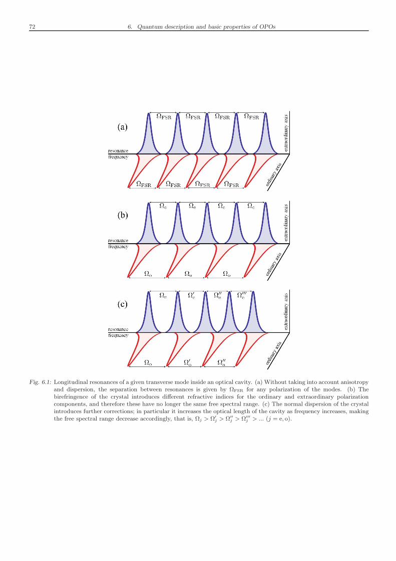
72 6. Quantum description and basic properties of OPOs

Fig. 6.1: Longitudinal resonances of a given transverse mode inside an optical cavity. (a) Without taking into account anisotropyand dispersion, the separation between resonances is given by ΩFSR for any polarization of the modes. (b) Thebirefringence of the crystal introduces different refractive indices for the ordinary and extraordinary polarizationcomponents, and therefore these have no longer the same free spectral range. (c) The normal dispersion of the crystalintroduces further corrections; in particular it increases the optical length of the cavity as frequency increases, makingthe free spectral range decrease accordingly, that is, Ωj > Ω′

j > Ω′′j > Ω′′′

j > ... (j = e, o).

6.1. Dielectric media and nonlinear optics 73

which is the generalization of the linear dispersion that we introduced in the previous section. We note, however, thatthis nonlinear dispersion is not as relevant as the normal dispersion appearing in the linear case, and one can safelyignore it within a fairly broad spectral region [94].

Similarly to the linear susceptibility, ←→χ (2)(ω;ω1, ω2) might be complex, although it also has to satisfy

←→χ (2)(−ω;−ω1,−ω2) = [←→χ (2)(ω;ω1, ω2)]∗. (6.19)

In any case, when absorption is neglected it can be proved to be real [93]. A number of general properties of the

χ(2)jkl(ω;ω1, ω2) coefficients upon permutation of its Cartesian or frequency arguments can also be proved [93]. For the

case of a lossless medium that we will consider, the most general of these is the one called full permutation symmetry,

which states that χ(2)jkl(ω;ω1, ω2) is left unchanged upon permutation of two frequency arguments, as long as the

Cartesian indices are permuted accordingly, that is,

χ(2)jkl(ω;ω1, ω2) = χ

(2)jlk(ω;ω2, ω1) = χ

(2)lkj(ω2;ω1,−ω) = ...; (6.20)

these relations will be useful in the next section.It is time now to see how the phenomenon of frequency conversion appears. To this aim, let us build now the wave

equation satisfied by the electric field, which is easily found to be

[

∇2 − µ0

←→ε ∂2t]

E (r, t) = −µ0∂2tP

(2) (r, t) , (6.21)

from the “rotational Maxwell’s equations” (the equations involving ∇ × E and ∇ × B). Imagine that we introduce

a wave of frequency ω0 in the medium. As we have shown, this wave induces a nonlinear polarization P(2)j (r, 2ω0) =

ε0χ(2)jkl(2ω0;ω0, ω0)Ek (r, ω0)El (r, ω0) in the medium oscillating at frequency 2ω0, and hence the wave equation for

the field component oscillating at that frequency will be

[

∇2 + 4ω2

0µ0←→ε]

Ej (r, 2ω0) = 4ω20µ0P

(2)j (r, 2ω0) ; (6.22)

this clearly shows that P(2) (r, 2ω0) acts as a source for a new wave which will oscillate at frequency 2ω0. Thisphenomenon is known as second harmonic generation. It is a particular case of the phenomenon known as frequencysum generation, in which the wave oscillating at frequency 2ω0 is generated from two waves of frequencies ω1 and ω2

satisfying ω1 + ω2 = 2ω0. All these effects are known as up–conversion, as the generated wave has a frequency largerthan the initial ones.

One can think about the opposite kind of process, down–conversion, in which a wave of frequency ω0 is generatedfrom an initial wave oscillating at frequency 2ω0. Note however, that this process is mediated by the nonlinear

polarization term P(2)j (r, ω0) = ε0χ

(2)jkl(ω0; 2ω0,−ω0)Ek (r, 2ω0) E

∗l (r, ω0), which is zero if the ω0 wave E (r, ω0) is

zero initially. Hence, the phenomenon of down–conversion cannot happen without some kind of initial seed. Whenthis initial seed is not an externally injected wave, but rather some initial fluctuations in the system (e.g., some smallamount of thermal photons), the process is known as spontaneous parametric down–conversion (the term “parametric”has a rather obscure origin that we won’t worry about).

In general, the down–conversion process might not be frequency degenerate, and hence two waves oscillating atfrequencies ω1 and ω2 are spontaneously generated from the initial wave of frequency 2ω0 = ω1 + ω2. In a down–conversion context, it is customary to call signal and idler to these two waves5, and pump to the 2ω0 wave. We willstick with this nomenclature, as most of the thesis (and certainly this chapter) deals with down–conversion processes.

As we will see when we develop their quantum theory, all this processes (collectively known as three–wave mixingprocesses) can be intuitively understood as a conversion of a pair of photons of frequencies ωs, ωi into one photon offrequency ωp = ωs+ωi, or vice versa. The dielectric medium acts just as a host, it doesn’t take any active involvementin the conversion process; hence, the energy and momentum of the photons must be conserved. Conservation of theenergy is granted by the delta–function appearing in (6.17). On the other hand, conservation of the linear momentumrequires one further condition, namely

npkp = nsks + niki, (6.23)

being nj the refractive index of the medium for the corresponding wave and kj = ωj/c its wave vector (in the followingwe assume that the three waves propagate in the same direction, what is known as collinear three–wave mixing, but

5 Which one is the signal or idler is not relevant. This nomenclature comes from the case in which one of the waves, say that of frequencyω1, is injected as a seed, and hence the other is generated through the frequency–difference generation process 2ω0 − ω1 → ω2. In thiscase, the injected wave is the signal, while the nonlinearly generated one is the idler.

74 6. Quantum description and basic properties of OPOs

everything we say applies for any other scheme). This condition is known as the phase–matching condition, and wewill show how it appears rigorously in the quantum description of the process (next section).

Consider a situation in which the three waves (pump, signal, and idler) have the same polarization, or in whichthe nonlinear medium does not show birefringence6, so that all the different polarization components of the field feelthe same refractive index; in such cases the phase–matching condition can be recasted as

ωi

ωs= −n(ωp)− n(ωs)

n(ωp)− n(ωi). (6.24)

The right hand side of this expression is always negative because, as follows from the normal dispersion commentedabove, n(ωp) > n(ωs), n(ωi); hence in order to conserve linear momentum the three waves involved in the down–conversion process cannot have the same polarization, and the medium must show birefringence.

As commented above, we will work with uniaxial media, although the phase–matching condition can also besatisfied in biaxial media too. For definiteness, and without loss of generalization, let us assume that ωs > ωi (wechoose the higher frequency wave of the signal–idler pair as the signal), and that the extraordinary refractive index islarger than the ordinary one 7, that is, ne(ω) > no(ω); in this case the pump (signal) wave has to be polarized alongthe ordinary (extraordinary) axis so that the numerator on the right hand side of (6.24) can become positive, that is,the phase–matching condition becomes

ne(ωs)− no(ωp)

no(ωp)− ni=ωi

ωs. (6.25)

We can distinguish then two types of processes. In a type I process both signal and idler have the same polarization(extraordinary with our conventions), while in a type II process they have orthogonal polarizations (extraordinary thesignal and ordinary the idler with our conventions).

Note that when signal and idler are frequency degenerate, the phase matching conditions are reduced to

[type I] ne(ω0) = no(2ω0), (6.26a)

[type II] ne(ω0) = 2no(2ω0)− no(ω0). (6.26b)

Hence, we see that the conditions for frequency degenerate processes are quite critical, they require a fine tuning of thecrystal parameters (as well as a proper stabilization of the cavity resonances in the case of working inside an opticalresonator, as we will).

Note finally that it may seem that the frequencies of the signal and idler waves are completely fixed by thefrequency we choose for the pump wave and the refractive indices of the crystal, so that in order to change to differentdown–conversion frequencies we may need to change either the pump frequency, or the crystal we are working with.Fortunately, the conditions (6.25) and (6.26) are much more flexible than they look, because the refractive indices ofthe crystal depend on the temperature in a known (or at least tabulated) way. Hence, even for a fixed pump frequency,one can still achieve the phase–matching condition for a desired signal–idler frequency pair by tuning the refractiveindices of the crystal8 via temperature tuning.

6.2 Quantum model for a general optical parametric oscillator

In order to optimize the frequency conversion process, it is customary to embed the nonlinear crystal in an opticalcavity, so that, e.g. for down–conversion, if one pump photon is not transformed into a signal–idler pair when it firstcrosses the crystal, it is reflected back in order to have one more chance to be down–converted. This system consistingof a χ(2)–crystal inside a resonator is known as optical parametric oscillator (OPO).

From the previous chapters we know how to treat quantum mechanically an optical cavity. The only question leftin order to analyze OPOs within that framework is which intracavity Hamiltonian Hc (in the notation of Chapter 4)

6 Actually, there is only one example of a crystalline class which does not have an inversion center (and hence, has second–ordersusceptibility), but does not show birefringence: the class 42m [93], to which for example Gallium arsenide belongs.

7 In general, an uniaxial crystal is called positive if ne > no, and negative in the opposite case. Although we assume to work withpositive uniaxial crystals, everything that we say is readily generalized to the negative case.

8 Another well known method to tune the phase–matching condition is by making a rotation θ of the crystal around the ordinarydirection eo. Under these circumstances, the polarization component of the field parallel to this direction will still feel a refractive indexno. However, the polarization component orthogonal to this direction won’t be parallel to the extraordinary direction anymore, and henceit will feel an effective refractive index n′

e given by [93]

1

n′e

=cos2 θ

ne+

sin2 θ

no

For reasons that will become obvious along the next chapters, we will assume during most of this thesis that no angular tuning is needed.

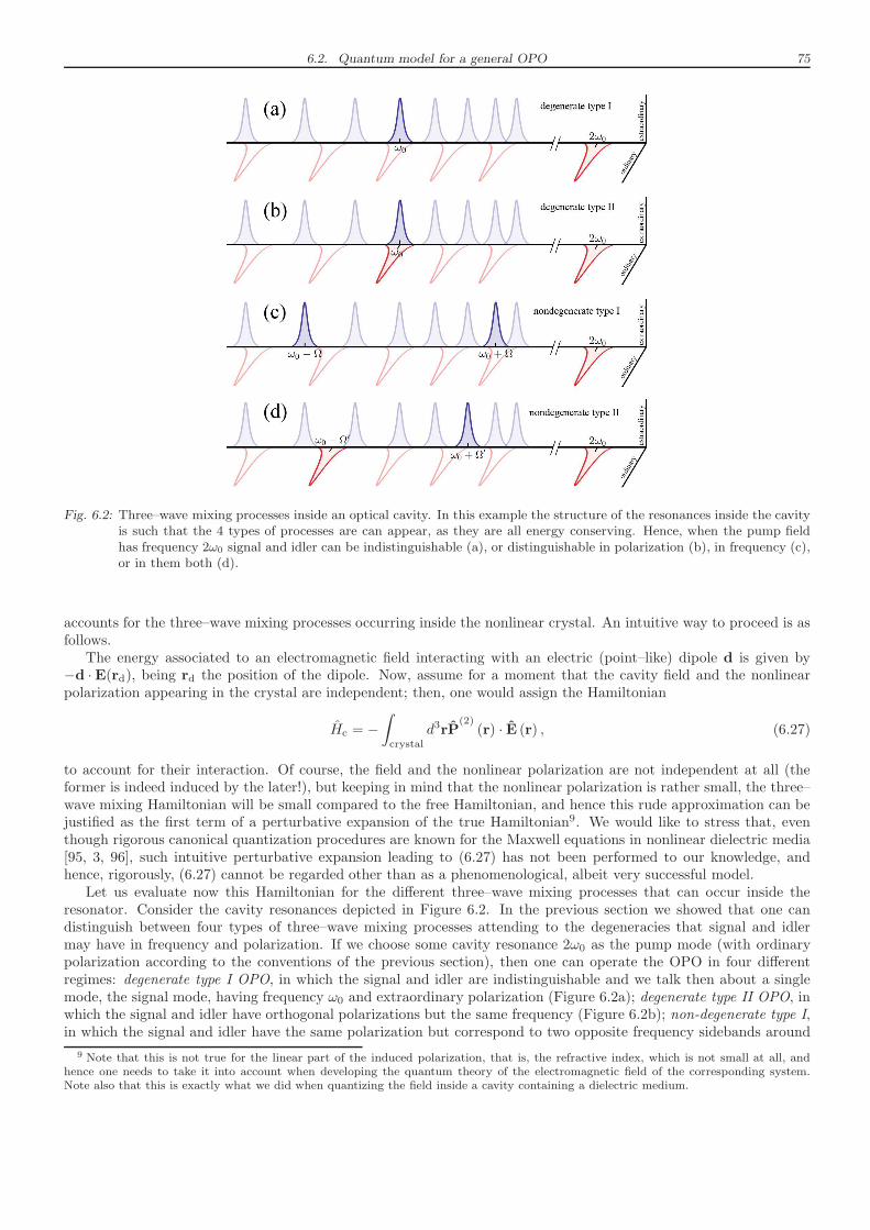
6.2. Quantum model for a general OPO 75

Fig. 6.2: Three–wave mixing processes inside an optical cavity. In this example the structure of the resonances inside the cavityis such that the 4 types of processes are can appear, as they are all energy conserving. Hence, when the pump fieldhas frequency 2ω0 signal and idler can be indistinguishable (a), or distinguishable in polarization (b), in frequency (c),or in them both (d).

accounts for the three–wave mixing processes occurring inside the nonlinear crystal. An intuitive way to proceed is asfollows.

The energy associated to an electromagnetic field interacting with an electric (point–like) dipole d is given by−d ·E(rd), being rd the position of the dipole. Now, assume for a moment that the cavity field and the nonlinearpolarization appearing in the crystal are independent; then, one would assign the Hamiltonian

Hc = −∫

crystal

d3rP(2)

(r) · E (r) , (6.27)

to account for their interaction. Of course, the field and the nonlinear polarization are not independent at all (theformer is indeed induced by the later!), but keeping in mind that the nonlinear polarization is rather small, the three–wave mixing Hamiltonian will be small compared to the free Hamiltonian, and hence this rude approximation can bejustified as the first term of a perturbative expansion of the true Hamiltonian9. We would like to stress that, eventhough rigorous canonical quantization procedures are known for the Maxwell equations in nonlinear dielectric media[95, 3, 96], such intuitive perturbative expansion leading to (6.27) has not been performed to our knowledge, andhence, rigorously, (6.27) cannot be regarded other than as a phenomenological, albeit very successful model.

Let us evaluate now this Hamiltonian for the different three–wave mixing processes that can occur inside theresonator. Consider the cavity resonances depicted in Figure 6.2. In the previous section we showed that one candistinguish between four types of three–wave mixing processes attending to the degeneracies that signal and idlermay have in frequency and polarization. If we choose some cavity resonance 2ω0 as the pump mode (with ordinarypolarization according to the conventions of the previous section), then one can operate the OPO in four differentregimes: degenerate type I OPO, in which the signal and idler are indistinguishable and we talk then about a singlemode, the signal mode, having frequency ω0 and extraordinary polarization (Figure 6.2a); degenerate type II OPO, inwhich the signal and idler have orthogonal polarizations but the same frequency (Figure 6.2b); non-degenerate type I,in which the signal and idler have the same polarization but correspond to two opposite frequency sidebands around

9 Note that this is not true for the linear part of the induced polarization, that is, the refractive index, which is not small at all, andhence one needs to take it into account when developing the quantum theory of the electromagnetic field of the corresponding system.Note also that this is exactly what we did when quantizing the field inside a cavity containing a dielectric medium.

76 6. Quantum description and basic properties of OPOs

ω0 (Figure 6.2c); and non-degenerate type II, in which the signal and idler are distinguishable both in frequency andpolarization (Figure 6.2d).

We can evaluate the Hamiltonian (6.27) for the four processes altogether. To do so, let us write the electric fieldas

E (r) = E(+)p (r) + (1− δsi/2)E(+)

s (r) + (1− δsi/2)E(+)i (r) + H.c., (6.28)

where E(+)p,s,i (r) are the (Schrodinger picture) electric fields associated to the pump, signal, and idler cavity modes

involved in the three–wave mixing process, and the factors (1− δsi/2) are introduced to include also the case in whichsignal and idler are indistinguishable (in which case δsi = 1), that is, the degenerate type I process.

The pump field has always ωp = 2ω0 and ordinary polarization (with the conventions of the previous section); onthe other hand, the signal field has always extraordinary polarization, but its frequency is different for the degenerate(Figures 6.2a and 6.2b) and non-degenerate (Figures 6.2c and 6.2d) schemes; finally, the polarization and frequency ofthe idler field depend on the particular three–wave mixing scheme. Hence, based on (3.100a) we can write the differentfrequency components of the field as

E(+)p (r) = i

√

~ωp

4ε0npLpeoap

[

G(kp; r⊥, z)einpkpz + c.c.

]

, (6.29a)

E(+)s (r) = i

√

~ωs

4ε0nsLsee∑

n

as,n[

Tn(ks; r⊥, z)einsksz + c.c.

]

, (6.29b)

E(+)i (r) = i

√

~ωi

4ε0niLiεi∑

n

ai,n[

Tn(ki; r⊥, z)einikiz + c.c.

]

, (6.29c)

where Lj is the optical length of the cavity evaluated for the refractive index seen by the corresponding mode, andthe polarization of the idler mode εi is left unspecified. Note that we have assumed that at the cavity resonance 2ω0

there exists only a TEM00 mode, which is denoted by G(k; r⊥, z), while several transverse modes Tn(k; r⊥, z)n canresonate at the signal and idler frequencies (the same for both, as this is the situation that we will find along thisthesis). We denote by ap, as,n, and ai,n, the intracavity annihilation operators for pump, signal, and idler photons,respectively.

As for the nonlinear polarization, we can also write it as

P(2) (r, t) = P(+)p (r) + (1− δsi/2)P(+)

s (r) + (1− δsi/2)P(+)i (r) + H.c., (6.30)

where, based on the previous section, we have10

P(+)p (r) = (2− δωs,ωi

)ε0χ(2)jlm(ωp;ωs, ωi)ej [E

(+)s (r)]l[E

(+)i (r)]m, (6.31a)

P(+)s (r) = 2ε0χ

(2)jlm(ωs;ωp,−ωi)ej [E

(+)p (r)]l[E

(−)i (r)]m, (6.31b)

P(+)i (r) = 2ε0χ

(2)jlm(ωi;ωp,−ωs)ej [E

(+)p (r)]l[E

(−)s (r)]m, (6.31c)

or in terms of the boson operators

P(+)p (r) = −(2− δωs,ωi

)

√

~2ωsωi

16nsniLsLiε0χ

(2)jem(ωp;ωs, ωi)ej [εi]m

∑

nm

as,nai,m (6.32a)

×[

Tn(ks; r⊥, z)Tm(ki; r⊥, z)ei(nsks+niki)z + Tn(ks; r⊥, z)T

∗m(ki; r⊥, z)e

i(nsks−niki)z + c.c.]

,

P(+)s (r) = 2

√

~2ωpωi

16npniLpLiε0χ

(2)jom(ωs;ωp,−ωi)ej [εi]m

∑

n

apa†i,n (6.32b)

×[

G(kp; r⊥, z)T∗n(ki; r⊥, z)e

i(npkp−niki)z +G(kp; r⊥, z)Tn(ki; r⊥, z)ei(npkp+niki)z + c.c.

]

,

P(+)i (r) = 2

√

~2ωpωs

16npnsLpLsε0χ

(2)joe(ωi;ωp,−ωs)ej

∑

n

apa†s,n (6.32c)

×[

G(kp; r⊥, z)T∗n(ks; r⊥, z)e

i(npkp−nsks)z +G(kp; r⊥, z)Tn(ks; r⊥, z)ei(npkp+nsks)z + c.c.

]

.

10 The factors 2 come because, for example P(+)s (r), receives contributions both from χ

(2)jlm(ωs;ωp,−ωi) and χ

(2)jlm(ωs;−ωi, ωp); this

contributions are easily shown to be the same by making use of full permutation symmetry.

6.2. Quantum model for a general OPO 77

Neglecting counter–rotating terms such as P(+)j (r) · E(+)

l (r) or P(−)p (r) · E(+)

s (r), and taking into account that by fullpermutation symmetry

χ(2)oej(ωp;ωs, ωi) = χ

(2)eoj(−ωs;−ωp, ωi) = χ

(2)joe(−ωi;−ωp, ωs), (6.33)

it is not difficult to write the Hamiltonian as

Hc = i~∑

nm

χnmapa†s,na

†i,m +H.c., (6.34)

where the coupling parameters are given by

χnm = χ(2)oej(ωp;ωs, ωi) [εi]j

√

~ωpωsωi

16ε0npnsniLpLsLi(3− δsi − δωs,ωi

/2)Inm, (6.35)

and we have defined the three–mode overlapping integral

Inm =

∫

crystal

d3r[

G(kp; r⊥, z)T∗n(ks; r⊥, z)T

∗m(ki; r⊥, z)e

i∆kz +G(kp; r⊥, z)T∗n(ks; r⊥, z)Tm(ki; r⊥, z)e

i∆k1z (6.36)

+G∗(kp; r⊥, z)T∗n(ks; r⊥, z)Tm(ki; r⊥, z)e

i∆k2z +G∗(kp; r⊥, z)T∗n(ks; r⊥, z)T

∗m(ki; r⊥, z)e

i∆k3z]

+ c.c.,

with

∆k = npkp − nsks − niki, ∆k1 = npkp − nsks + niki, (6.37)

∆k2 = −npkp − nsks + niki, ∆k3 = −npkp − nsks − niki.

Just as we stated in the previous section, this Hamiltonian shows how the three–wave mixing process is describedfrom a quantum viewpoint as the annihilation of a pump photon and the simultaneous creation of a signal–idler pair,or vice versa. In order for the process to be efficient, we need the three–mode–overlapping integral to be as large aspossible; let us now simplify the model a little bit in order to understand under which conditions Inm is maximized.

Assume that the center of the crystal coincides with the cavity’s waist plane, and that its length lc is muchsmaller than the Rayleigh length of the resonator, that is, lc ≪ zR, see after (3.42). Under these circumstances, thelongitudinal variation of the transverse modes can be neglected inside the crystal, see (3.87), and therefore all thelongitudinal integrals in Inm are of the form

∫ lc/2

−lc/2

dzei∆kjz = lcsinc

(

∆kj lc2

)

; (6.38)

hence, we see that in order to maximize the conversion process, some of the ∆kj ’s must satisfy |∆kj | ≪ l−1c . Onthe other hand, ∆k = 0 is precisely the phase matching condition that we introduced in the previous section usinglinear momentum conservation arguments, and hence, we assume now that ∆k ≪ l−1c ; under these conditions, it iscompletely trivial to show that the rest of ∆kj ’s are all well above l−1c , so that their contribution to Inm can beneglected.

The Hamiltonian can be even more simplified if we choose the Laguerre–Gauss basis for the transverse modes(3.47), which are written in the cavity waist as

Lpl (k; r⊥, z = 0) = R|l|p (k; r) exp [ilφ] , (6.39)

with

R|l|p (k; r) =

√

2p!

π (p+ |l|)!1

w

(√2r

w

)|l|

L|l|p

(

2r2

w2

)

exp

(

− r2

w2

)

, (6.40)

being w the spot size of the modes at the cavity waist. The interesting thing about these modes is that they areeigenfunctions of the orbital angular momentum operator, that is, −i∂φLpl (k; r⊥, z) = lLpl (k; r⊥, z), and henceconservation of this quantity in the conversion process should appear explicitly in this basis. In particular, takinginto account the phase matching condition ∆k ≪ l−1c that we have already selected, in the Laguerre–Gauss basis thethree–mode overlapping integral reads

Ipl,p′l′ = 2lcδ−ll′

∫ +∞

0

rdrG(kp ; r)R|l|p (ks; r)R|l′|p′ (ki; r), (6.41)

78 6. Quantum description and basic properties of OPOs

and hence the three–wave mixing Hamiltonian takes the final form

Hc = i~∑

pp′,l≥0

χlpp′ apa†s,p,la

†i,p′,−l +H.c., (6.42)

where the sum extend over all the opposite orbital angular momentum pairs present at the signal–idler cavityresonances, and

χlpp′ =3− δsi − δωs,ωi

/2

1 + δl,0lcχ

(2)oej(ωp;ωs, ωi) [εi]j

√

~ωpωsωi

ε0npnsniLpLsLi

∫ +∞

0

rdrG(kp; r)Rlp(ks; r)Rlp′ (ki; r). (6.43)

Let us remark at this point that, ideally, we can decide which of the possible intracavity three–wave mixingprocesses is selected by operating the OPO in the corresponding phase matching condition. In most of the thesis wewill assume that this is the case. In practice, however, one can select between type I and II at will, but additional caremust be taken in order to ensure working with a desired pair of signal–idler frequencies around ω0, or the degeneratefrequency ω0 itself. We shall come back to this issue in the next chapter.

We have now at our disposal a quantum model for a general OPO. Note that in the case of indistinguishablesignal and idler, Hc is similar to the Hamiltonian that we used to generate squeezed states of the harmonic oscillator,see (2.31). Similarly, when signal and idler are distinguishable, the Hamiltonian resembles the one which producedentangled states (2.39). Hence, the OPO seems a perfect candidate for the generation of squeezed and entangled statesof light. The rest of the chapter is devoted to analyze these properties of the light generated by the OPO.

6.3 Squeezing properties of the DOPO

In this section we study the squeezing properties of degenerate type I OPOs (DOPOs). To this purpose, let us workwith the simplest transverse mode configuration, in which we consider only a TEM00 mode resonating at the signalfrequency. Squeezing in OPOs was originally predicted by using this single–mode DOPO model [97]11, and throughoutthis thesis we will learn under which conditions it is valid.

The analysis performed in this section is of major importance for this thesis, as any other OPO configuration willbe analyzed with simple adaptations of it.

6.3.1 The DOPO within the positive P representation

The single–mode DOPO deals then with two cavity modes only: The pump mode, which resonates at frequency ωp =2ω0 and has ordinary polarization, and the signal mode, which resonates at frequency ωs = ω0 and has extraordinarypolarization (Figure 6.2a). Both are in a TEM00 transverse mode. The pump mode is driven by an external laserbeam of frequency 2ωL close to 2ω0, while no injection is used for the signal mode; hence, signal photons are expectedto appear from the pump field via spontaneous parametric down–conversion.

In Figure 6.3 it is shown the basic experimental scheme used to pump and detect the DOPO. Note that the samelaser is used both as the injection for the cavity (after doubling its frequency) and as the local oscillator field, whichensures that all the phases of the system are more or less locked. Based on the analysis of homodyne detectionintroduced in the previous chapter, we move then to the interaction picture defined by the transformation operator

U0 = exp[H0t/i~] with H0 = ~ωL

(

2a†pap + a†s as)

, (6.44)

that is, we “rotate” the system to the local oscillator (or injection) frequency. The state ρ of the intracavity modes is

written as ρI = U †0 ρU0 in this picture, and satisfies the master equation

dρIdt

=[

−2i∆a†pap − i∆a†s as +χ

2apa†2s + Epa†p +H.c., ρI

]

+∑

j=p,s

γj(2aj ρIa†j − a

†j aj ρI − ρIa

†j aj), (6.45)

11 The story of such prediction was actually quite intricate [1]. The problem was that the first analyses of squeezing in OPOs wereperformed not in terms of the noise spectrum of the field coming out from the cavity, but in terms of the uncertainties of the intracavitymodes, which showed only a 50% noise reduction even in the most ideal situation [98, 99]. Hence, these initial predictions were alittle disappointing, since such small levels of squeezing couldn’t help much for the applications of squeezing proposed at that time[100, 101, 102, 103]. The puzzle was finally solved by Collet and Gardiner [97], who applied the input–output formalism previouslyintroduced by Yurke and Denker in electronic circuits [104], to analyze the field coming out from the parametric oscillator in terms of itssqueezing spectrum.

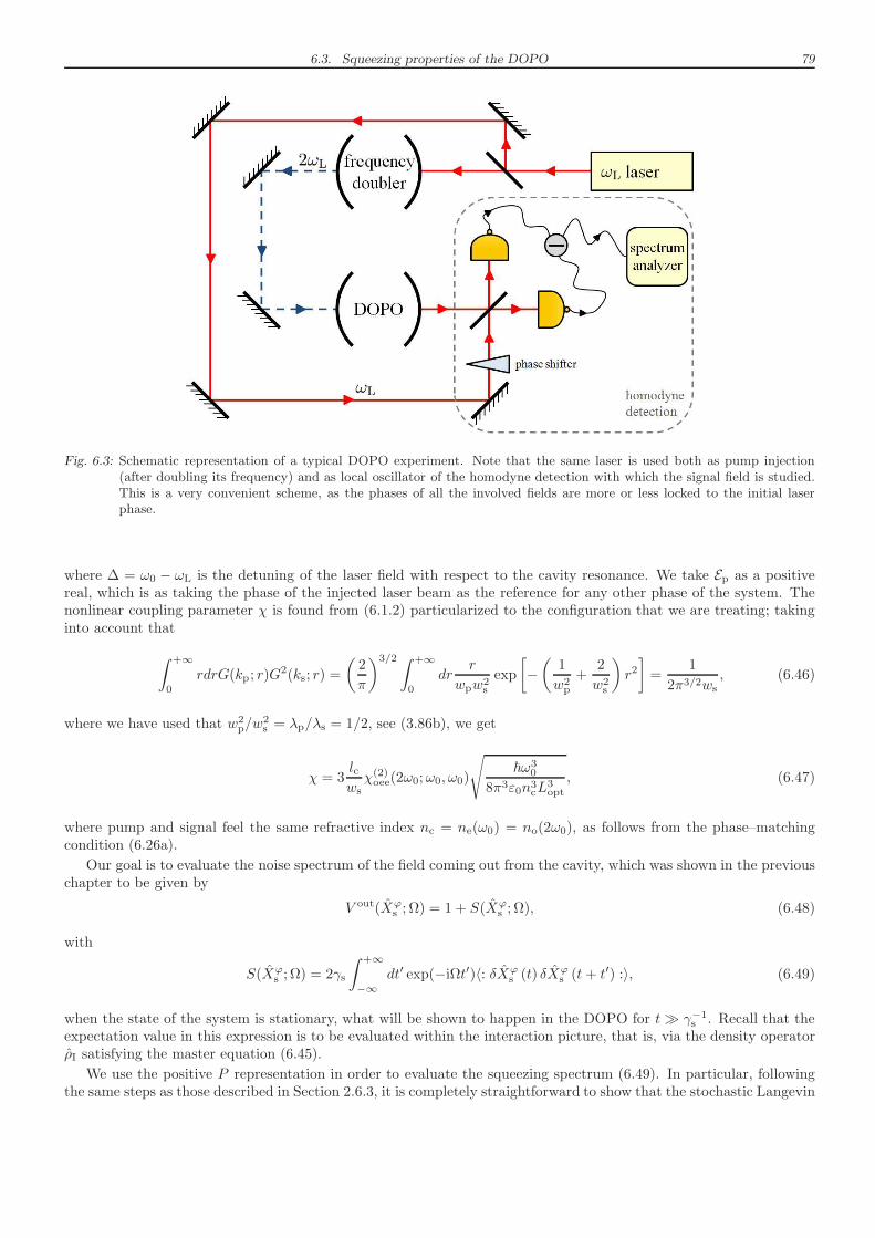
6.3. Squeezing properties of the DOPO 79

Fig. 6.3: Schematic representation of a typical DOPO experiment. Note that the same laser is used both as pump injection(after doubling its frequency) and as local oscillator of the homodyne detection with which the signal field is studied.This is a very convenient scheme, as the phases of all the involved fields are more or less locked to the initial laserphase.

where ∆ = ω0 − ωL is the detuning of the laser field with respect to the cavity resonance. We take Ep as a positivereal, which is as taking the phase of the injected laser beam as the reference for any other phase of the system. Thenonlinear coupling parameter χ is found from (6.1.2) particularized to the configuration that we are treating; takinginto account that

∫ +∞

0

rdrG(kp; r)G2(ks; r) =

(

2

π

)3/2 ∫ +∞

0

drr

wpw2s

exp

[

−(

1

w2p

+2

w2s

)

r2]

=1

2π3/2ws, (6.46)

where we have used that w2p/w

2s = λp/λs = 1/2, see (3.86b), we get

χ = 3lcwsχ(2)oee(2ω0;ω0, ω0)

√

~ω30

8π3ε0n3cL

3opt

, (6.47)

where pump and signal feel the same refractive index nc = ne(ω0) = no(2ω0), as follows from the phase–matchingcondition (6.26a).

Our goal is to evaluate the noise spectrum of the field coming out from the cavity, which was shown in the previouschapter to be given by

V out(Xϕs ; Ω) = 1 + S(Xϕ

s ; Ω), (6.48)

with

S(Xϕs ; Ω) = 2γs

∫ +∞

−∞

dt′ exp(−iΩt′)〈: δXϕs (t) δXϕ

s (t+ t′) :〉, (6.49)

when the state of the system is stationary, what will be shown to happen in the DOPO for t≫ γ−1s . Recall that theexpectation value in this expression is to be evaluated within the interaction picture, that is, via the density operatorρI satisfying the master equation (6.45).

We use the positive P representation in order to evaluate the squeezing spectrum (6.49). In particular, followingthe same steps as those described in Section 2.6.3, it is completely straightforward to show that the stochastic Langevin

80 6. Quantum description and basic properties of OPOs

equations associated to the master equation (6.45) are

αp = Ep − (γp + i∆)αp −χ

2α2s , (6.50a)

α+p = Ep − (γp − i∆)α+

p −χ

2α+2s , (6.50b)

αs = −(γs + i∆)αs + χαpα+s +√χαpη(t), (6.50c)

α+s = −(γs − i∆)α+

s + χα+p αs +

√

χα+p η

+(t), (6.50d)

where η(t) and η+(t) are independent real Gaussian noises which satisfy the usual statistical properties (2.82). Eventhough noise is multiplicative in these equations, it is easy to show that they have the same form both within the Itoand Stratonovich interpretations, and hence we can directly use the usual rules of calculus to analyze them.

In order to better appreciate the parameters needed to model the system, we will make the following variablechange

τ = γst, βm(τ) =χ

γs√

γp/γmαm(t), ζm(τ) =

1√γsηm(t), (6.51)

where with these definitions the new noises ζ(τ) and ζ+(τ) satisfy the same statistical properties as η(t) and η+(t),but now with respect to the dimensionless time τ . In terms of these scaled variables, the Langevin equations (6.50)read (derivatives with respect to τ are understood)

βp = κ[σ − (1 + i∆)βp − β2s /2] (6.52a)

β+p = κ[σ − (1− i∆)β+

p − β+2s /2] (6.52b)

βs = −(1 + i∆)βs + βpβ+s + g

√

βpζ(τ) (6.52c)

β+s = −(1− i∆)β+

s + β+p βs + g

√

β+p ζ

+(τ), (6.52d)

which have only four dimensionless parameters

κ = γp/γs, ∆ = ∆/γs, σ = χEp/γpγs, g = χ/√γpγs, (6.53)

which are, respectively, normalized versions of the pump’s damping rate, the detuning, the pump injection parameter,and the nonlinear coupling. In the following we will set ∆ = 0 for simplicity; we will analyze the effects of detuningin Section 6.3.4.

These equations allow us to evaluate the squeezing spectrum as

S(Xϕs ; Ω) =

2

g2

∫ +∞

−∞

dτ ′ exp(−iΩτ ′)〈δxϕs (τ) δxϕs (τ + τ ′)〉P , (6.54)

where we have defined normalized versions of the noise frequency Ω = Ω/γs and the quadratures within the positiveP phase representation

xϕs (τ) = e−iϕβs (τ) + eiϕβ+s (τ) . (6.55)

Hence, in order to evaluate the squeezing spectrum we need the solutions βm(τ) of (6.52) in terms of the noises, sothat from them we can evaluate the corresponding stochastic averages. However, these equations are a set of couplednonlinear stochastic equations, and hence it is impossible to perform this task analytically without introducing furtherapproximations. Let us first show the behavior of the DOPO in the classical limit, and then we will come back to theproblem of solving (6.52).

6.3.2 Classical analysis of the DOPO

Before studying the quantum properties of any OPO, it is convenient to analyze what classical optics has to say aboutits dynamics. In the next section we will see that this is not only convenient, but also mandatory in order to extractanalytic information from its quantum model. Moreover, along the thesis, and starting in the next section, we willlearn how to predict the quantum properties of OPOs just from a qualitative understanding of their classical behavior.

In principle, the classical behavior of the field inside an OPO must be studied by using the nonlinear wave equationof the electric field (6.21) with appropriate boundary conditions accounting for the (open) cavity. There is a simplerroute though. From the chapter where we studied the harmonic oscillator, we learned that quantum predictions

6.3. Squeezing properties of the DOPO 81

become equivalent to the classical description of the system in a certain limit. We introduced the coherent states ofthe oscillator as those which allowed for these quantum–to–classical transition; the interesting thing to note aboutcoherent states is that there are no quantum correlations on them, that is, given two oscillators with annihilationoperators a1 and a2 both in some coherent state, it is satisfied

⟨

a21⟩

= 〈a1〉 〈a1〉 and 〈a1a2〉 = 〈a1〉 〈a2〉 , (6.56)

for example. Hence, one way to retrieve the classical equations from the evolution equations for the operators of thesystem is to take expectation values, and decorrelate any product of operators following (6.56), which is as using acoherent ansatz for the state of the system. The quantities νj =

√

2~/ωj 〈aj〉 are then identified with the normalvariables of the various harmonic oscillators that form the system, being ωj their natural oscillation frequency. Thisprocedure is called the mean field limit.

Equipped with an stochastic quantum model for the system, the classical limit is even simpler to devise. Theidea now is that the classical behavior of the system (its classical phase–space trajectory) should be recovered whenquantum noise is negligible. Hence, the classical equations of an OPO should be recovered by neglecting the noiseterms on its corresponding Langevin equations, and identifying νj =

√

2~/ωjαj with the normal variables of the cavitymodes. When using the positive P representation there is one more prescription though: In order to come back to aclassical phase space, the variables α+

j of the extended phase space have to be identified with α∗j . This procedure isin agreement with (and completely equivalent to) the mean field scenario discussed above.

Applying these ideas to our DOPO model (6.52), we get the following classical equations

βp = κ(

σ − βp − β2s /2)

, (6.57a)

βs = −βs + βpβ∗s . (6.57b)

This is a set of first–order nonlinear differential equations, which, again, cannot be solved analytically. Fortunately,there is actually no need for doing so for our purposes. One is usually interested only on the long time term solutionsthat these equations predict for the system. In particular, the first type of solutions that one needs to look for arethe so-called stationary or steady state solutions, in which the variables do not depend on time. These solutions arefound by setting βp = βs = 0, then arriving to a simple algebraic system

σ = βp + β2s /2, (6.58a)

βs = βpβ∗s . (6.58b)

This system admits two types of such solutions. In the first type the signal mode is switched off, and hence we have

βp = σ and βs = 0, (6.59)

where the overbar is used to denote “classical long time term solution”. In the second type, the signal mode is switchedon, and in order to find the explicit form of the solution we use the following amplitude–phase representation of thevariables: βj = ρj exp(iϕj). From the second equation we trivially get ρp = 1 and exp(iϕp) = exp(2iϕs), whichintroduced in the first equation leads to ρs =

√σ − 1 and ϕs = 0, π, that is,

βp = 1 and βs = ±√

2 (σ − 1). (6.60)

Note that this second solution only exists for σ ≥ 1; we say that the domain of existence of the solutions are all theparameter space σ, κ and the region σ ≥ 1, κ for the first and second solutions, respectively. Note also that atσ = 1 both solutions coincide.

Knowing the possible solutions of (6.58) in the long time term is not enough. It can happen that a solution existsbut is unstable, that is, an arbitrarily small perturbation can make the system move out from that solution and fall intoanother solution. It is not difficult to analyze the stability of a solution. With full generality, consider the equation

β = f (β) , (6.61)

where all the complex variables of the system are collected as

β = (β1, β∗1 , β2, β

∗2 , ..., βN , β

∗N ), (6.62)

and one stationary solution β satisfying f(

β)

= 0. In order to see whether this solution is stable or not, we justintroduce a small perturbation b (τ) in the system and analyze how it grows. Writing β(τ) = β + b (τ), and making

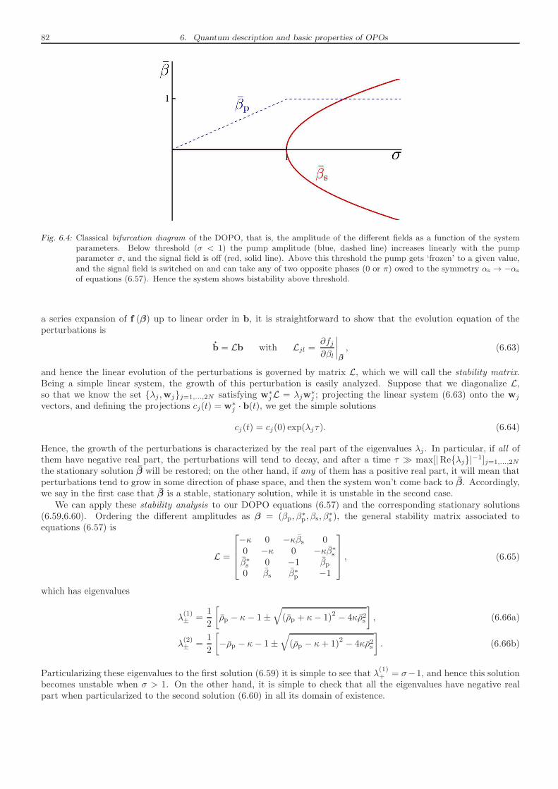
82 6. Quantum description and basic properties of OPOs

Fig. 6.4: Classical bifurcation diagram of the DOPO, that is, the amplitude of the different fields as a function of the systemparameters. Below threshold (σ < 1) the pump amplitude (blue, dashed line) increases linearly with the pumpparameter σ, and the signal field is off (red, solid line). Above this threshold the pump gets ‘frozen’ to a given value,and the signal field is switched on and can take any of two opposite phases (0 or π) owed to the symmetry αs → −αs

of equations (6.57). Hence the system shows bistability above threshold.

a series expansion of f (β) up to linear order in b, it is straightforward to show that the evolution equation of theperturbations is

b = Lb with Ljl =∂fj∂βl

∣

∣

∣

∣

β

, (6.63)

and hence the linear evolution of the perturbations is governed by matrix L, which we will call the stability matrix.Being a simple linear system, the growth of this perturbation is easily analyzed. Suppose that we diagonalize L,so that we know the set λj ,wjj=1,...,2N satisfying w∗jL = λjw

∗j ; projecting the linear system (6.63) onto the wj

vectors, and defining the projections cj(t) = w∗j · b(t), we get the simple solutions

cj(t) = cj(0) exp(λjτ). (6.64)

Hence, the growth of the perturbations is characterized by the real part of the eigenvalues λj . In particular, if all ofthem have negative real part, the perturbations will tend to decay, and after a time τ ≫ max[|Reλj|−1]j=1,...,2N

the stationary solution β will be restored; on the other hand, if any of them has a positive real part, it will mean thatperturbations tend to grow in some direction of phase space, and then the system won’t come back to β. Accordingly,we say in the first case that β is a stable, stationary solution, while it is unstable in the second case.

We can apply these stability analysis to our DOPO equations (6.57) and the corresponding stationary solutions(6.59,6.60). Ordering the different amplitudes as β = (βp, β

∗p, βs, β

∗s ), the general stability matrix associated to

equations (6.57) is

L =

−κ 0 −κβs 00 −κ 0 −κβ∗sβ∗s 0 −1 βp0 βs β∗p −1

, (6.65)

which has eigenvalues

λ(1)± =

1

2

[

ρp − κ− 1±√

(ρp + κ− 1)2 − 4κρ2s

]

, (6.66a)

λ(2)± =

1

2

[

−ρp − κ− 1±√

(ρp − κ+ 1)2 − 4κρ2s

]

. (6.66b)

Particularizing these eigenvalues to the first solution (6.59) it is simple to see that λ(1)+ = σ−1, and hence this solution

becomes unstable when σ > 1. On the other hand, it is simple to check that all the eigenvalues have negative realpart when particularized to the second solution (6.60) in all its domain of existence.

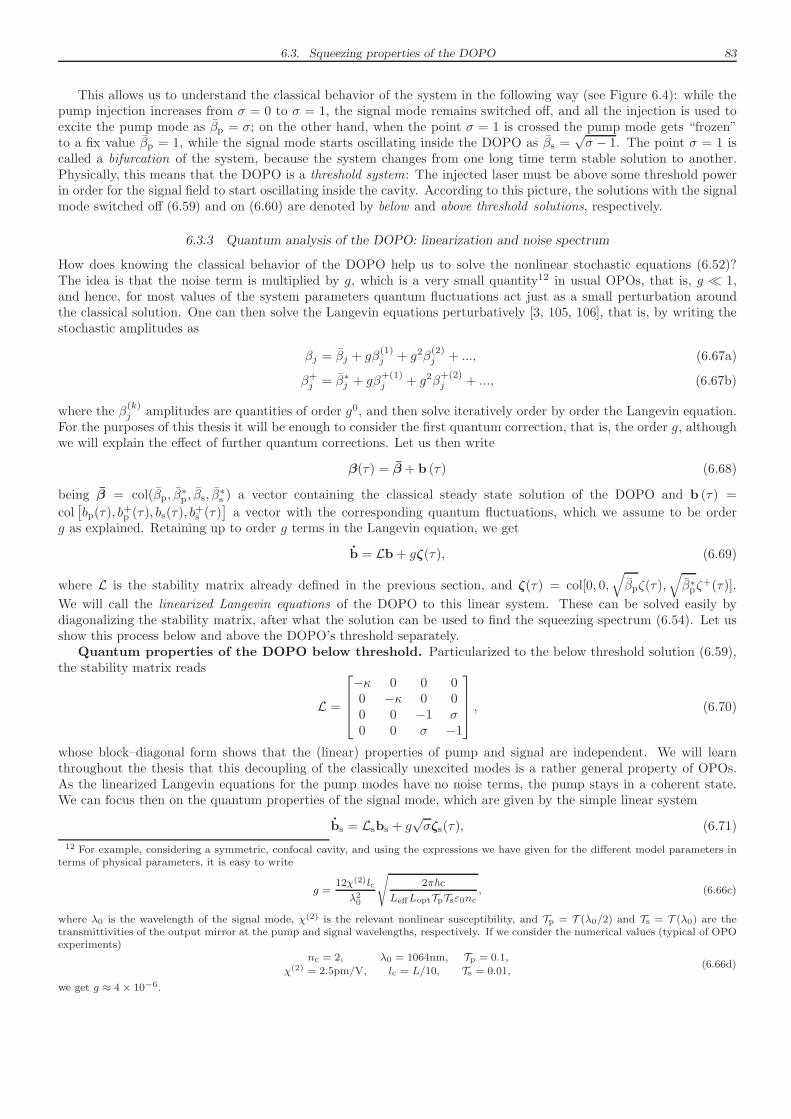
6.3. Squeezing properties of the DOPO 83

This allows us to understand the classical behavior of the system in the following way (see Figure 6.4): while thepump injection increases from σ = 0 to σ = 1, the signal mode remains switched off, and all the injection is used toexcite the pump mode as βp = σ; on the other hand, when the point σ = 1 is crossed the pump mode gets “frozen”to a fix value βp = 1, while the signal mode starts oscillating inside the DOPO as βs =

√σ − 1. The point σ = 1 is

called a bifurcation of the system, because the system changes from one long time term stable solution to another.Physically, this means that the DOPO is a threshold system: The injected laser must be above some threshold powerin order for the signal field to start oscillating inside the cavity. According to this picture, the solutions with the signalmode switched off (6.59) and on (6.60) are denoted by below and above threshold solutions, respectively.

6.3.3 Quantum analysis of the DOPO: linearization and noise spectrum

How does knowing the classical behavior of the DOPO help us to solve the nonlinear stochastic equations (6.52)?The idea is that the noise term is multiplied by g, which is a very small quantity12 in usual OPOs, that is, g ≪ 1,and hence, for most values of the system parameters quantum fluctuations act just as a small perturbation aroundthe classical solution. One can then solve the Langevin equations perturbatively [3, 105, 106], that is, by writing thestochastic amplitudes as

βj = βj + gβ(1)j + g2β

(2)j + ..., (6.67a)

β+j = β∗j + gβ

+(1)j + g2β

+(2)j + ..., (6.67b)

where the β(k)j amplitudes are quantities of order g0, and then solve iteratively order by order the Langevin equation.

For the purposes of this thesis it will be enough to consider the first quantum correction, that is, the order g, althoughwe will explain the effect of further quantum corrections. Let us then write

β(τ) = β + b (τ) (6.68)

being β = col(βp, β∗p, βs, β

∗s ) a vector containing the classical steady state solution of the DOPO and b (τ) =

col[

bp(τ), b+p (τ), bs(τ), b

+s (τ)

]

a vector with the corresponding quantum fluctuations, which we assume to be orderg as explained. Retaining up to order g terms in the Langevin equation, we get

b = Lb+ gζ(τ), (6.69)

where L is the stability matrix already defined in the previous section, and ζ(τ) = col[0, 0,√

βpζ(τ),√

β∗pζ+(τ)].

We will call the linearized Langevin equations of the DOPO to this linear system. These can be solved easily bydiagonalizing the stability matrix, after what the solution can be used to find the squeezing spectrum (6.54). Let usshow this process below and above the DOPO’s threshold separately.

Quantum properties of the DOPO below threshold. Particularized to the below threshold solution (6.59),the stability matrix reads

L =

−κ 0 0 00 −κ 0 00 0 −1 σ0 0 σ −1

, (6.70)

whose block–diagonal form shows that the (linear) properties of pump and signal are independent. We will learnthroughout the thesis that this decoupling of the classically unexcited modes is a rather general property of OPOs.As the linearized Langevin equations for the pump modes have no noise terms, the pump stays in a coherent state.We can focus then on the quantum properties of the signal mode, which are given by the simple linear system

bs = Lsbs + g√σζs(τ), (6.71)

12 For example, considering a symmetric, confocal cavity, and using the expressions we have given for the different model parameters interms of physical parameters, it is easy to write

g =12χ(2)lc

λ20

√

2π~c

LeffLoptTpTsε0nc, (6.66c)

where λ0 is the wavelength of the signal mode, χ(2) is the relevant nonlinear susceptibility, and Tp = T (λ0/2) and Ts = T (λ0) are thetransmittivities of the output mirror at the pump and signal wavelengths, respectively. If we consider the numerical values (typical of OPOexperiments)

nc = 2, λ0 = 1064nm, Tp = 0.1,

χ(2) = 2.5pm/V, lc = L/10, Ts = 0.01,(6.66d)

we get g ≈ 4× 10−6.

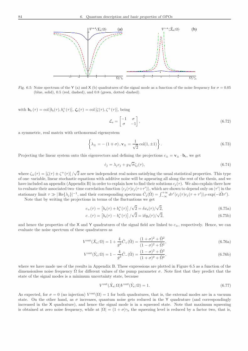
84 6. Quantum description and basic properties of OPOs

Fig. 6.5: Noise spectrum of the Y (a) and X (b) quadratures of the signal mode as a function of the noise frequency for σ = 0.05(blue, solid), 0.5 (red, dashed), and 0.8 (green, dotted–dashed).

with bs (τ) = col [bs(τ), b+s (τ)], ζs(τ) = col [ζ(τ), ζ+(τ)], being

Ls =[

−1 σσ −1

]

, (6.72)

a symmetric, real matrix with orthonormal eigensystem

λ± = − (1∓ σ) ,v± =1√2col(1,±1)

. (6.73)

Projecting the linear system onto this eigenvectors and defining the projections c± = v± · bs, we get

cj = λjcj + g√σζj(τ), (6.74)

where ζ±(τ) = [ζ(τ) ± ζ+(τ)] /√2 are new independent real noises satisfying the usual statistical properties. This type

of one–variable, linear stochastic equations with additive noise will be appearing all along the rest of the thesis, and wehave included an appendix (Appendix B) in order to explain how to find their solutions cj(τ). We also explain there howto evaluate their associated two–time correlation function 〈cj(τ)cj(τ+τ ′)〉, which are shown to depend only on |τ ′| in the

stationary limit τ ≫ |Reλj|−1, and their corresponding spectrum Cj(Ω) =∫ +∞

−∞dτ ′〈cj(τ)cj(τ + τ ′)〉P exp(−iΩτ ′).

Note that by writing the projections in terms of the fluctuations we get

c+(τ) =[

bs(τ) + b+s (τ)]

/√2 = δxs(τ)/

√2, (6.75a)

c−(τ) =[

bs(τ)− b+s (τ)]

/√2 = iδys(τ)/

√2, (6.75b)

and hence the properties of the X and Y quadratures of the signal field are linked to c±, respectively. Hence, we canevaluate the noise spectrum of these quadratures as

V out(Xs; Ω) = 1 +4

g2C+(Ω) =

(1 + σ)2 + Ω2

(1− σ)2 + Ω2, (6.76a)

V out(Ys; Ω) = 1− 4

g2C−(Ω) =

(1− σ)2 + Ω2

(1 + σ)2 + Ω2, (6.76b)

where we have made use of the results in Appendix B. These expressions are plotted in Figure 6.5 as a function of thedimensionless noise frequency Ω for different values of the pump parameter σ. Note first that they predict that thestate of the signal modes is a minimum uncertainty state, because

V out(Xs; Ω)Vout(Ys; Ω) = 1. (6.77)

As expected, for σ = 0 (no injection) V out(Ω) = 1 for both quadratures, that is, the external modes are in a vacuumstate. On the other hand, as σ increases, quantum noise gets reduced in the Y quadrature (and correspondinglyincreased in the X quadrature), and hence the signal mode is in a squeezed state. Note that maximum squeezingis obtained at zero noise frequency, while at |Ω| = (1 + σ)γs the squeezing level is reduced by a factor two, that is,

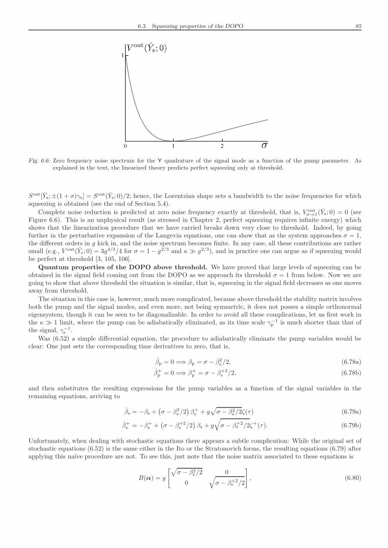
6.3. Squeezing properties of the DOPO 85

Fig. 6.6: Zero frequency noise spectrum for the Y quadrature of the signal mode as a function of the pump parameter. Asexplained in the text, the linearized theory predicts perfect squeezing only at threshold.

Sout[Ys;±(1 + σ)γs] = Sout(Ys; 0)/2; hence, the Lorentzian shape sets a bandwidth to the noise frequencies for whichsqueezing is obtained (see the end of Section 5.4).

Complete noise reduction is predicted at zero noise frequency exactly at threshold, that is, V outσ→1(Ys; 0) = 0 (see

Figure 6.6). This is an unphysical result (as stressed in Chapter 2, perfect squeezing requires infinite energy) whichshows that the linearization procedure that we have carried breaks down very close to threshold. Indeed, by goingfurther in the perturbative expansion of the Langevin equations, one can show that as the system approaches σ = 1,the different orders in g kick in, and the noise spectrum becomes finite. In any case, all these contributions are rathersmall (e.g., V out(Ys; 0) = 3g4/3/4 for σ = 1− g2/3 and κ≫ g2/3), and in practice one can argue as if squeezing wouldbe perfect at threshold [3, 105, 106].

Quantum properties of the DOPO above threshold. We have proved that large levels of squeezing can beobtained in the signal field coming out from the DOPO as we approach its threshold σ = 1 from below. Now we aregoing to show that above threshold the situation is similar, that is, squeezing in the signal field decreases as one movesaway from threshold.

The situation in this case is, however, much more complicated, because above threshold the stability matrix involvesboth the pump and the signal modes, and even more, not being symmetric, it does not posses a simple orthonormaleigensystem, though it can be seen to be diagonalizable. In order to avoid all these complications, let us first work inthe κ ≫ 1 limit, where the pump can be adiabatically eliminated, as its time scale γ−1p is much shorter than that ofthe signal, γ−1s .

Was (6.52) a simple differential equation, the procedure to adiabatically eliminate the pump variables would beclear: One just sets the corresponding time derivatives to zero, that is,

βp = 0 =⇒ βp = σ − β2s /2, (6.78a)

β+p = 0 =⇒ β+

p = σ − β+2s /2, (6.78b)

and then substitutes the resulting expressions for the pump variables as a function of the signal variables in theremaining equations, arriving to

βs = −βs +(

σ − β2s /2)

β+s + g

√

σ − β2s /2ζ(τ) (6.79a)

β+s = −β+

s +(

σ − β+2s /2

)

βs + g

√

σ − β+2s /2ζ+(τ). (6.79b)

Unfortunately, when dealing with stochastic equations there appears a subtle complication: While the original set ofstochastic equations (6.52) is the same either in the Ito or the Stratonovich forms, the resulting equations (6.79) afterapplying this naıve procedure are not. To see this, just note that the noise matrix associated to these equations is

B(α) = g

[√

σ − β2s /2 0

0√

σ − β+2s /2

]

, (6.80)

86 6. Quantum description and basic properties of OPOs

so that the terms which connect the Ito and Stratonovich forms (2.86) read

1

2

∑

lm

Blm (βs) ∂lBβsm (βs) =1

2Bβsβs

(βs) ∂βsBβsβs

(βs) = −g2

4βs, (6.81a)

1

2

∑

lm

Blm (βs) ∂lBβ+s m

(βs) =1

2Bβ+

s β+s(βs) ∂β+

sBβ+

s β+s(βs) = −

g2

4β+s , (6.81b)

which are different from zero. Hence it is fair to ask within which interpretation is this “deterministic” procedurecorrect, if it is correct at all. Using the techniques explained in [61] to perform the adiabatic elimination in theFokker–Planck equation (where there are no problems of interpretation), it is possible to show that this procedure isindeed correct within Ito’s interpretation. Hence, the corresponding Stratonovich equations have additional terms inthe deterministic part, and in particular they read

βs = −(1− g2/4)βs +(

σ − β2s /2)

β+s + g

√

σ − β2s /2ζ(τ), (6.82a)

β+s = −

(

1− g2/4)

β+s +

(

σ − β+2s /2

)

βs + g

√

σ − β+2s /2ζ+(τ). (6.82b)

Note that the difference between the Ito and Stratonovich forms of the equations is of order g2, and then disappearswhen making the linearization procedure; in particular, the linearized equations read in this case

bs = Lsbs + gζs(τ), (6.83)

with bs (τ) = col [bs(τ), b+s (τ)], ζs(τ) = col [ζ(τ), ζ+(τ)], being

Ls =[

1− 2σ 11 1− 2σ

]

, (6.84)

a symmetric, real matrix with orthonormal eigensystem

λ+ = −2 (σ − 1) , v+ =1√2col(1, 1), (6.85a)

λ− = −2σ, v− =1√2col(1,−1). (6.85b)

Note also that the eigenvectors are the same as the ones below threshold, and hence they have the same relationto the quadrature fluctuations of the signal modes (7.12). Then, by following the same procedure as before, thatis, by projecting the linear system (6.83) onto the eigensystem of Ls and evaluating the correlation spectrum of theprojections c± = v± · bs, it is straightforward to find the following expressions for the noise spectrum of the X and Y

quadratures of the signal field

V out(Xs; Ω) = 1 +1

(σ − 1)2 +Ω2/4, (6.86a)

V out(Ys; Ω) = 1− 1

σ2 +Ω2/4. (6.86b)

These have again a Lorentzian shape, and, as already stated at the beginning of the present section, they predict perfectsqueezing in the Y quadrature at zero noise frequency only at threshold (as before, the complete noise reduction comesfrom the linearization, and nonlinear corrections in the g parameter give rise to finite squeezing levels [106]). As σincreases this squeezing is lost (see Figure 6.6), with the particularity that now the state of the signal is no longer aminimum uncertainty state, because

V out(Xs; Ω)Vout(Ys; Ω) > 1, (6.87)

for σ > 1.

6.3.4 Effect of signal detuning

In the previous sections we have analyzed the classical and quantum behavior of the DOPO when everything is onresonance, that is, the frequency ωL of the external laser and its second harmonic coincide with the phase–matchedcavity resonances ω0 and 2ω0, the signal and pump frequencies. Here we just want to show the effect that detuning

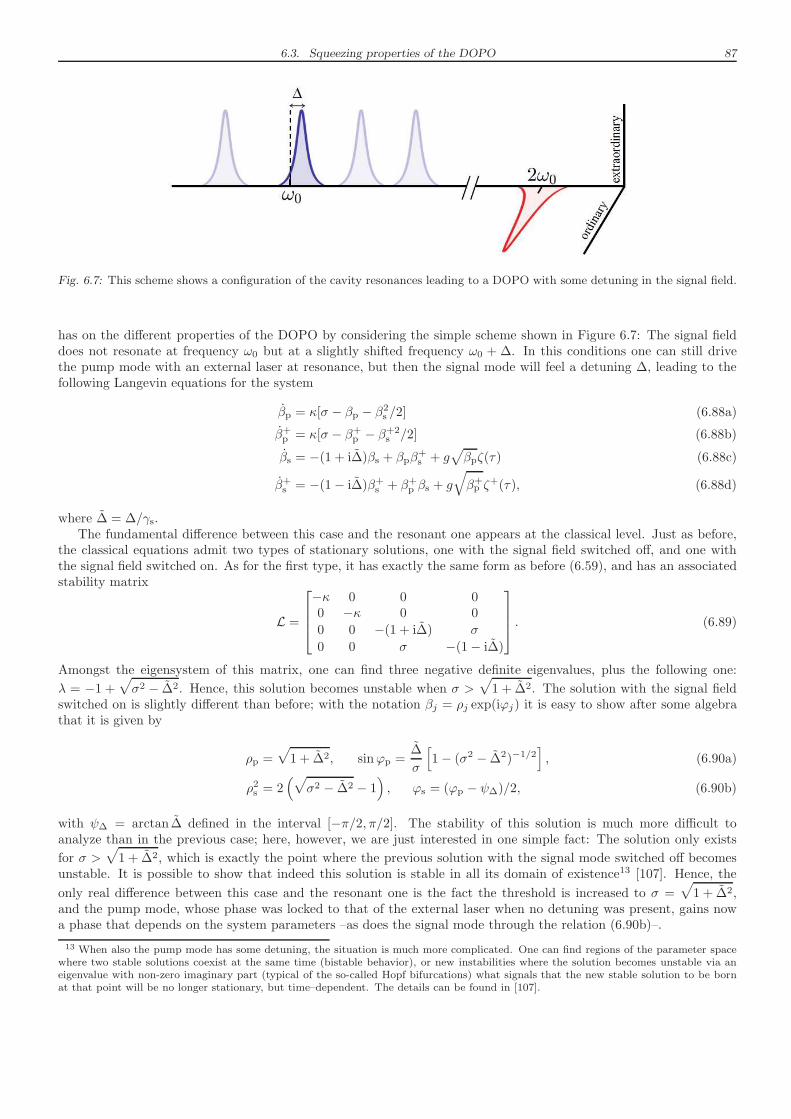
6.3. Squeezing properties of the DOPO 87

Fig. 6.7: This scheme shows a configuration of the cavity resonances leading to a DOPO with some detuning in the signal field.

has on the different properties of the DOPO by considering the simple scheme shown in Figure 6.7: The signal fielddoes not resonate at frequency ω0 but at a slightly shifted frequency ω0 + ∆. In this conditions one can still drivethe pump mode with an external laser at resonance, but then the signal mode will feel a detuning ∆, leading to thefollowing Langevin equations for the system

βp = κ[σ − βp − β2s /2] (6.88a)

β+p = κ[σ − β+

p − β+2s /2] (6.88b)

βs = −(1 + i∆)βs + βpβ+s + g

√

βpζ(τ) (6.88c)

β+s = −(1− i∆)β+

s + β+p βs + g

√

β+p ζ

+(τ), (6.88d)

where ∆ = ∆/γs.The fundamental difference between this case and the resonant one appears at the classical level. Just as before,

the classical equations admit two types of stationary solutions, one with the signal field switched off, and one withthe signal field switched on. As for the first type, it has exactly the same form as before (6.59), and has an associatedstability matrix

L =

−κ 0 0 00 −κ 0 0

0 0 −(1 + i∆) σ

0 0 σ −(1− i∆)

. (6.89)

Amongst the eigensystem of this matrix, one can find three negative definite eigenvalues, plus the following one:

λ = −1 +√

σ2 − ∆2. Hence, this solution becomes unstable when σ >√

1 + ∆2. The solution with the signal fieldswitched on is slightly different than before; with the notation βj = ρj exp(iϕj) it is easy to show after some algebrathat it is given by

ρp =√

1 + ∆2, sinϕp =∆

σ

[

1− (σ2 − ∆2)−1/2]

, (6.90a)

ρ2s = 2(√

σ2 − ∆2 − 1)

, ϕs = (ϕp − ψ∆)/2, (6.90b)

with ψ∆ = arctan ∆ defined in the interval [−π/2, π/2]. The stability of this solution is much more difficult toanalyze than in the previous case; here, however, we are just interested in one simple fact: The solution only exists

for σ >√

1 + ∆2, which is exactly the point where the previous solution with the signal mode switched off becomesunstable. It is possible to show that indeed this solution is stable in all its domain of existence13 [107]. Hence, the

only real difference between this case and the resonant one is the fact the threshold is increased to σ =√

1 + ∆2,and the pump mode, whose phase was locked to that of the external laser when no detuning was present, gains nowa phase that depends on the system parameters –as does the signal mode through the relation (6.90b)–.

13 When also the pump mode has some detuning, the situation is much more complicated. One can find regions of the parameter spacewhere two stable solutions coexist at the same time (bistable behavior), or new instabilities where the solution becomes unstable via aneigenvalue with non-zero imaginary part (typical of the so-called Hopf bifurcations) what signals that the new stable solution to be bornat that point will be no longer stationary, but time–dependent. The details can be found in [107].

88 6. Quantum description and basic properties of OPOs

As for the squeezing properties of the signal field, nothing is fundamentally changed: It is simple to show byfollowing the procedure developed in the previous sections that there exists a squeezed quadrature which showsperfect noise reduction exactly at threshold, the squeezing level degrading as one moves away from this point [107].The only subtlety which appears is that phase of the squeezed quadrature is no longer π/2, but depends on the σ and∆ parameters [107].

6.4 Entanglement properties of the OPO

We study now the quantum properties of an OPO having distinguishable signal and idler modes (in polarizationor/and frequency); from now on we will call OPO (in contrast to DOPO) to any such configuration. To this aim, letus work again with the simplest situation: only a fundamental TEM00 transverse mode is present at the signal andidler resonances, so we are dealing with a so-called two–mode OPO.

We will see that, similarly to the DOPO, the OPO is also a threshold system. Quantum properties can then bedivided in two classes:

(i) Below threshold the signal and idler modes are in an EPR-like entangled state. Although below threshold OPOswere studied before (see [99, 108] for example), Reid and Drummond were the first ones to notice that theEPR gedanken experiment could actually be implemented with such devices [109, 44, 110]. The first experimentalong this line was performed shortly after their proposal [111], and of course confirmed the quantum mechanicalpredictions.

(ii) Above threshold the signal and idler modes leak out of the cavity as two bright beams with (ideally) perfectlycorrelated intensities, usually referred to as twin beams. Such intensity correlations between macroscopicallyoccupied beams were first predicted [112] and experimentally observed [113] by Fabre et al. in Paris. Togetherwith the intensity correlations, and in order to preserve the corresponding Heisenberg uncertainty principle, thephase difference between the twin beams is diffusing. In many articles concerning above threshold OPOs suchphase diffusion is neglected; its effects on various properties of OPOs were first studied by Lane, Reid, and Walls[114] and by Reid and Drummond [109, 115]. In order to introduce twin beams in simple terms, we will notconsider phase diffusion in this chapter; such effect will be treated rigorously in Chapter 814.

6.4.1 The OPO within the positive P representation

Let us choose degenerate type II operation, as this is the ideal situation from the experimental viewpoint, becausethen the signal and idler fields can be analyzed using the same local oscillator field. In any case, the results that we aregoing to show are independent of the particular type of OPO. The two–mode OPO we are considering deals then withthree cavity modes: The pump mode which resonates at frequency ωp = 2ω0 and has ordinary polarization, and thesignal and idler modes which resonate at frequency ωs = ωi = ω0 and have extraordinary and ordinary polarization,respectively (Figure 6.2b). Every mode is assumed to be in a TEM00 transverse mode. The pump mode is driven byan external, resonant laser beam, while no injection is used for the signal and idler modes, whose associated photonsare then generated via spontaneous parametric down–conversion.

Similarly to the degenerate case, we move to the interaction picture defined by the transformation operator

U0 = exp[H0t/i~] with H0 = ~ωL(2a†pap + a†s as + a†i ai). (6.91)

In this picture, the state ρ of the intracavity modes is written as ρI = U †0 ρU0, and satisfies the master equation

dρIdt

=[

χapa†s a†i + Epa†p +H.c., ρI

]

+∑

j=p,s,i

γj(2aj ρIa†j − a

†j aj ρI − ρIa

†j aj), (6.92)

where we take γs = γi, what is a reasonable approximation from the experimental viewpoint. We take Ep as a positivereal as before. Once again, the nonlinear coupling parameter χ is found from (6.1.2) particularized to the configurationthat we are treating, which do not write explicitly because no real simplifications are obtained in this case.

14 Indeed, this phenomenon offers the perfect example of the usefulness of positive P techniques based on the master equation of thesystem (see Sections 2.6.3 and 4.3), as it cannot be studied by dealing with operator techniques such as that introduced in Section 4.2because an operator corresponding to the phase of the cavity modes is not available [23, 20].

6.4. Entanglement properties of the OPO 89

We use the positive P representation for the density operator, what in this case leads to the stochastic Langevinequations

αp = Ep − γpαp − χαsαi, (6.93a)

α+p = Ep − γpα+

p − χα+s α

+i , (6.93b)

αs = −γsαs + χαpα+i +√χαpξ(t), (6.93c)

α+s = −γsα+

s + χα+p αi +

√

χα+p ξ

+(t), (6.93d)

αi = −γsαi + χαpα+s +√χαpξ

∗(t), (6.93e)

α+i = −γsα+

i + χα+p αs +

√

χα+p [ξ

+(t)]∗, (6.93f)

where now ξ(t) and ξ+(t) are independent complex Gaussian noises with zero mean and non-zero correlations

〈ξ(t), ξ∗(t′)〉P = 〈ξ+(t), [ξ+(t′)]∗〉P = δ(t− t′). (6.94)

Once again, it is easy to show that these equations have the same form both within the Ito and Stratonovich inter-pretations, and hence we can directly use the usual rules of calculus to analyze them.

In order to simplify the equations, we will make the same variable change as in the DOPO,

τ = γst, βm(τ) =χ

γs√

γp/γmαm(t), ζm(τ) =

1√γsξm(t), (6.95)

where with these definitions the new noises ζ(τ) and ζ+(τ) satisfy the same statistical properties as ξ(t) and ξ+(t),but now with respect to the dimensionless time τ . In terms of these normalized variables, the Langevin equations(6.93) read (derivatives with respect to τ are understood)

βp = κ[σ − βp − βsβi], (6.96a)

β+p = κ[σ − β+

p − β+s β

+i ], (6.96b)

βs = −βs + βpβ+i + g

√

βpζ(τ), (6.96c)

β+s = −β+

s + β+p βi + g

√

β+p ζ

+(τ), (6.96d)

βi = −βi + βpβ+s + g

√

βpζ∗(τ), (6.96e)

β+i = −β+

i + β+p βs + g

√

β+p [ζ+(τ)]∗, (6.96f)

where the σ, κ, and g parameters have the same definition as before (6.53).In order to extract information from these equations we will proceed as before, that is, by linearizing them around

the classical stable solution.

6.4.2 Classical analysis of the OPO

Using the same procedure as in Section (6.3.2), we retrieve the classical evolution equations of the OPO, which read

βp = κ[σ − βp − βsβi], (6.97a)

βs = −βs + βpβ∗i , (6.97b)

βi = −βi + βpβ∗s . (6.97c)

Similarly to (6.57), these equations admit two types of solutions, one with the signal–idler modes switched off, andanother with all the modes switched on. Again, the first type exists for all the parameters, but becomes unstable forσ > 1, while the second type exists only for σ ≥ 1 and is stable in all its domain of existence. Note however, thatin this case these equations have the continuous symmetry βs → exp(−iθ)βs, βi → exp(iθ)βi, and hence the phasedifference between the signal and idler modes is not fixed by the classical equations (a result of paramount importancefor the results we derive later).

Explicitly, the stationary solution below threshold is

βp = σ, βs,i = 0, (6.98)

90 6. Quantum description and basic properties of OPOs

while now the above threshold stationary solution reads

βp = 1, βs,i =√σ − 1 exp(∓iθ), (6.99)

being θ arbitrary. The stability of these solutions is easily analyzed following the same steps as in (6.3.2), thatis, analyzing the sign of the real part of the eigenvalues of the stability matrix, and leads to the scenario alreadycommented above.

Let us finally discuss one point regarding what we could expect in real experiments. Assume that we operate theOPO above threshold. Bright signal and idler beams are then expected to start oscillating inside the cavity, theirrelative phase θ chosen randomly according to the particular fluctuations from which the beams are built up. Wesay then that θ is chosen by spontaneous symmetry breaking. In this chapter we assume that after this spontaneoussymmetry breaking process, the value of θ remains fixed; in reality, any source of noise (thermal, electronic, etc...) canmake it drift. We can assume all the classical sources of noise to be properly stabilized (at least within the time–scaleof the experiment), but even then, quantum noise will remain. Nevertheless, for the purposes of this introduction tothe properties of OPOs we will neglect this quantum phase diffusion phenomenon, which will be properly addressedalong the next chapters.

6.4.3 The OPO below threshold: Signal–idler entanglement

Linearizing now the Langevin equations (6.96) around the below threshold classical solution (6.98) we can prove thatthe quadratures of the signal and idler modes have correlations of the EPR type. In particular, we will prove that forσ > 0 these modes satisfy

V out[(Xs − Xi)/√2; Ω] < 1 and V out[(Ys + Yi)/

√2; Ω] < 1, (6.100)

which is to be regarded as the generalization of the entanglement criterion (2.38) to the free–space fields leaking outof the cavity. Moreover, we will show that these EPR like correlations become perfect exactly at threshold.

To this aim, let us expand the stochastic amplitudes of the modes as (6.68); it is straightforward to see that thelinear evolution of the signal/idler fluctuations is decoupled from the pump fluctuations, and obey the linear system

bsi = Lsibsi + g√σζsi(τ), (6.101)

with

bsi (τ) = col[

bs(τ), b+s (τ), bi(τ), b

+i (τ)

]

, (6.102a)

ζsi(τ) = colζ(τ), ζ+(τ), ζ∗(τ), [ζ+(τ)]∗, (6.102b)

being

Ls =

−1 0 0 σ0 −1 σ 00 σ −1 0σ 0 0 −1

, (6.103)

a symmetric, real matrix with orthonormal eigensystem

λ1 = −1− σ, v1 =1

2col(1, 1,−1,−1), (6.104a)

λ2 = −1− σ, v2 =1

2col(1,−1, 1,−1), (6.104b)

λ3 = 1− σ, v3 =1

2col(1, 1, 1, 1), (6.104c)

λ4 = 1− σ, v4 =1

2col(1,−1,−1, 1). (6.104d)

Once again, this linear system is solved by defining the projections cj(τ) = vj ·bsi (τ), which obey the following simplelinear stochastic equation with additive noise

c1,4 = λ1,4c1,4 + ig√σζ1,4(τ) (6.105a)

c2,3 = λ2,3c2,3 + g√σζ2,3(τ), (6.105b)

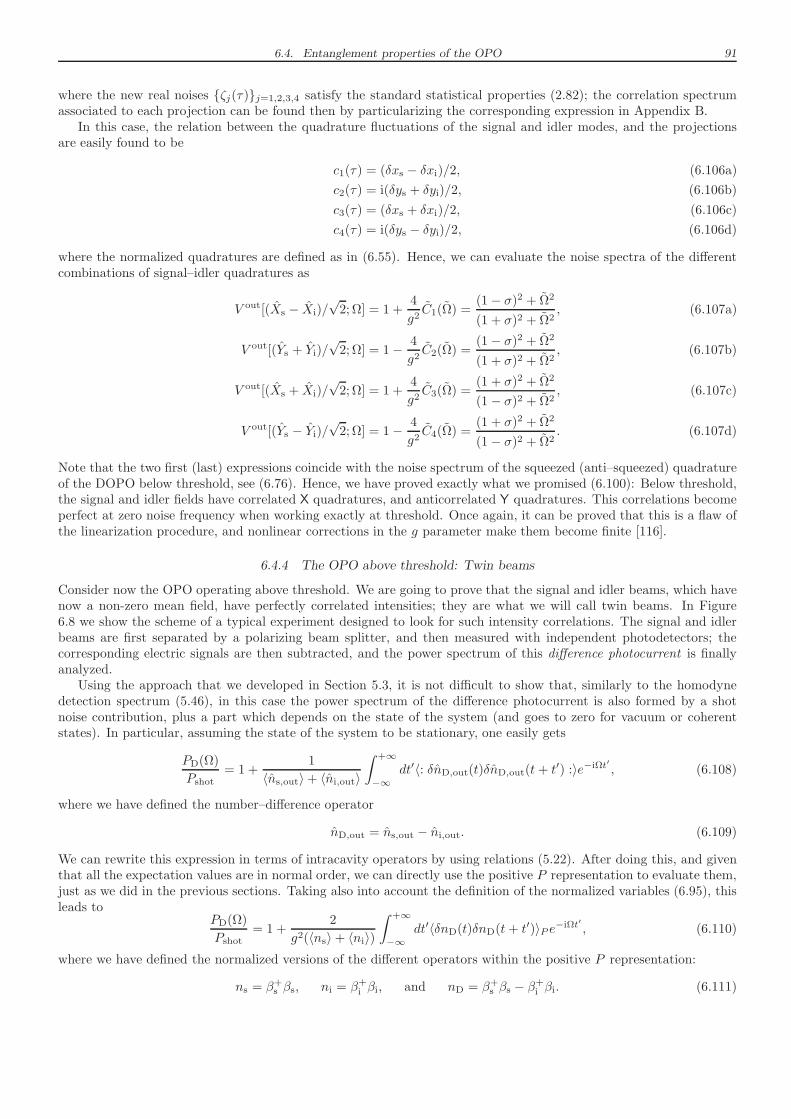
6.4. Entanglement properties of the OPO 91

where the new real noises ζj(τ)j=1,2,3,4 satisfy the standard statistical properties (2.82); the correlation spectrumassociated to each projection can be found then by particularizing the corresponding expression in Appendix B.

In this case, the relation between the quadrature fluctuations of the signal and idler modes, and the projectionsare easily found to be

c1(τ) = (δxs − δxi)/2, (6.106a)

c2(τ) = i(δys + δyi)/2, (6.106b)

c3(τ) = (δxs + δxi)/2, (6.106c)

c4(τ) = i(δys − δyi)/2, (6.106d)

where the normalized quadratures are defined as in (6.55). Hence, we can evaluate the noise spectra of the differentcombinations of signal–idler quadratures as

V out[(Xs − Xi)/√2; Ω] = 1 +

4

g2C1(Ω) =

(1 − σ)2 + Ω2

(1 + σ)2 + Ω2, (6.107a)

V out[(Ys + Yi)/√2; Ω] = 1− 4

g2C2(Ω) =

(1 − σ)2 + Ω2

(1 + σ)2 + Ω2, (6.107b)

V out[(Xs + Xi)/√2; Ω] = 1 +

4

g2C3(Ω) =

(1 + σ)2 + Ω2

(1 − σ)2 + Ω2, (6.107c)

V out[(Ys − Yi)/√2; Ω] = 1− 4

g2C4(Ω) =

(1 + σ)2 + Ω2

(1 − σ)2 + Ω2. (6.107d)

Note that the two first (last) expressions coincide with the noise spectrum of the squeezed (anti–squeezed) quadratureof the DOPO below threshold, see (6.76). Hence, we have proved exactly what we promised (6.100): Below threshold,the signal and idler fields have correlated X quadratures, and anticorrelated Y quadratures. This correlations becomeperfect at zero noise frequency when working exactly at threshold. Once again, it can be proved that this is a flaw ofthe linearization procedure, and nonlinear corrections in the g parameter make them become finite [116].

6.4.4 The OPO above threshold: Twin beams

Consider now the OPO operating above threshold. We are going to prove that the signal and idler beams, which havenow a non-zero mean field, have perfectly correlated intensities; they are what we will call twin beams. In Figure6.8 we show the scheme of a typical experiment designed to look for such intensity correlations. The signal and idlerbeams are first separated by a polarizing beam splitter, and then measured with independent photodetectors; thecorresponding electric signals are then subtracted, and the power spectrum of this difference photocurrent is finallyanalyzed.

Using the approach that we developed in Section 5.3, it is not difficult to show that, similarly to the homodynedetection spectrum (5.46), in this case the power spectrum of the difference photocurrent is also formed by a shotnoise contribution, plus a part which depends on the state of the system (and goes to zero for vacuum or coherentstates). In particular, assuming the state of the system to be stationary, one easily gets

PD(Ω)

Pshot= 1 +

1

〈ns,out〉+ 〈ni,out〉

∫ +∞

−∞

dt′〈: δnD,out(t)δnD,out(t+ t′) :〉e−iΩt′ , (6.108)

where we have defined the number–difference operator

nD,out = ns,out − ni,out. (6.109)

We can rewrite this expression in terms of intracavity operators by using relations (5.22). After doing this, and giventhat all the expectation values are in normal order, we can directly use the positive P representation to evaluate them,just as we did in the previous sections. Taking also into account the definition of the normalized variables (6.95), thisleads to

PD(Ω)

Pshot= 1 +

2

g2(〈ns〉+ 〈ni〉)

∫ +∞

−∞

dt′〈δnD(t)δnD(t+ t′)〉P e−iΩt′

, (6.110)

where we have defined the normalized versions of the different operators within the positive P representation:

ns = β+s βs, ni = β+

i βi, and nD = β+s βs − β+

i βi. (6.111)

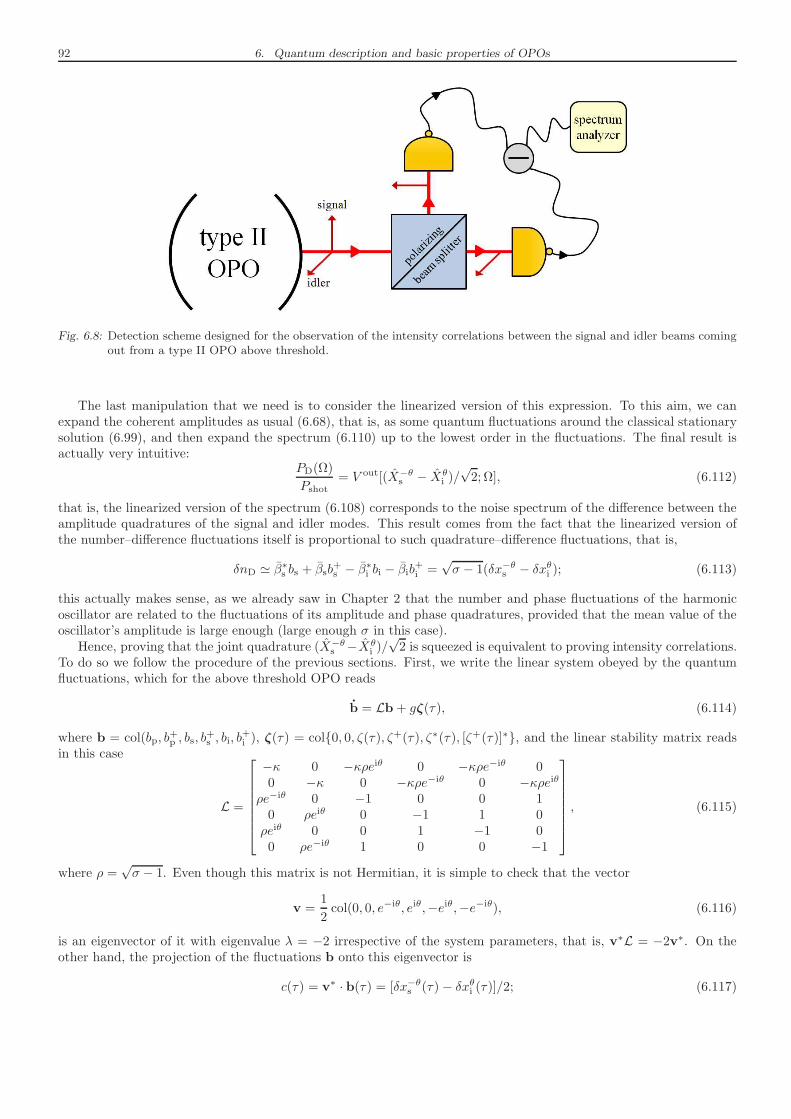
92 6. Quantum description and basic properties of OPOs

Fig. 6.8: Detection scheme designed for the observation of the intensity correlations between the signal and idler beams comingout from a type II OPO above threshold.

The last manipulation that we need is to consider the linearized version of this expression. To this aim, we canexpand the coherent amplitudes as usual (6.68), that is, as some quantum fluctuations around the classical stationarysolution (6.99), and then expand the spectrum (6.110) up to the lowest order in the fluctuations. The final result isactually very intuitive:

PD(Ω)

Pshot= V out[(X−θs − Xθ

i )/√2; Ω], (6.112)

that is, the linearized version of the spectrum (6.108) corresponds to the noise spectrum of the difference between theamplitude quadratures of the signal and idler modes. This result comes from the fact that the linearized version ofthe number–difference fluctuations itself is proportional to such quadrature–difference fluctuations, that is,

δnD ≃ β∗s bs + βsb+s − β∗i bi − βib+i =

√σ − 1(δx−θs − δxθi ); (6.113)

this actually makes sense, as we already saw in Chapter 2 that the number and phase fluctuations of the harmonicoscillator are related to the fluctuations of its amplitude and phase quadratures, provided that the mean value of theoscillator’s amplitude is large enough (large enough σ in this case).

Hence, proving that the joint quadrature (X−θs −Xθi )/√2 is squeezed is equivalent to proving intensity correlations.

To do so we follow the procedure of the previous sections. First, we write the linear system obeyed by the quantumfluctuations, which for the above threshold OPO reads

b = Lb+ gζ(τ), (6.114)

where b = col(bp, b+p , bs, b

+s , bi, b

+i ), ζ(τ) = col0, 0, ζ(τ), ζ+(τ), ζ∗(τ), [ζ+(τ)]∗, and the linear stability matrix reads

in this case

L =

−κ 0 −κρeiθ 0 −κρe−iθ 00 −κ 0 −κρe−iθ 0 −κρeiθ

ρe−iθ 0 −1 0 0 10 ρeiθ 0 −1 1 0ρeiθ 0 0 1 −1 00 ρe−iθ 1 0 0 −1

, (6.115)

where ρ =√σ − 1. Even though this matrix is not Hermitian, it is simple to check that the vector

v =1

2col(0, 0, e−iθ, eiθ,−eiθ,−e−iθ), (6.116)

is an eigenvector of it with eigenvalue λ = −2 irrespective of the system parameters, that is, v∗L = −2v∗. On theother hand, the projection of the fluctuations b onto this eigenvector is

c(τ) = v∗ · b(τ) = [δx−θs (τ) − δxθi (τ)]/2; (6.117)

6.4. Entanglement properties of the OPO 93

then, by projecting the linear system (6.114) onto v we get the evolution equation for this projection, which reads

c = −2c+ igη(t), (6.118)

where η(t) is a real noise which satisfies the usual statistics (2.82). As usual this is a linear stochastic equation withadditive noise, see Appendix B. Hence, the noise spectrum we are looking for can be finally written as

V out[(X−θs − Xθi )/√2; Ω] = 1 +

4

g2C(Ω) =

Ω2

4 + Ω2, (6.119)

where once again we have used the results of Appendix B for the correlation spectrum of c(τ).As stated, the signal and idler modes have perfect amplitude quadrature correlations above threshold (for any value

of the system parameters) and at zero noise frequency, what is equivalent to perfect intensity correlations as explainedabove. The shape of the spectrum is the usual Lorentzian that we have found for all the previous perfectly squeezedquadratures; however, as we show in Section ..., in this case this shape is not an unrealistic artifact of the linearization:the intensities (or amplitude quadratures) of the generated twin beams can be indeed perfectly correlated.

Let us finally remark that the vector (6.116) is not the only one with a definite eigenvalue in all parameter space;it is simple to check that the vector

v0 =i

2col(0, 0, e−iθ,−eiθ,−eiθ, e−iθ), (6.120)

satisfies v∗0L = 0, and hence has zero eigenvalue. This zero eigenvalue is an indicator that there is a direction of phasespace along which quantum noise can act freely. It is actually easy to realize which is the corresponding variableof the system affected by this undamped quantum noise; one just needs to evaluate the projection of the quantumfluctuations b onto v0, what leads to

c0(τ) = v∗0 · b(τ) = [δy−θs (τ)− δyθi (τ)]/2, (6.121)

that is, the difference between the phase quadratures of the signal and idler modes is the variable we are lookingfor. In other words, as within the linearized description the fluctuations of the phase quadrature are related to thefluctuations of the actual phase of the mode, the phase difference θ that we have taken as a fixed quantity of the abovethreshold solution, is actually dynamical, it should diffuse with time owed to quantum noise (as already advancedabove). Fortunately, it can be proved that adding this phase diffusion doesn’t change the results we have shownconcerning intensity correlations [114]; it however affects other aspects of above threshold OPOs that we haven’ttackled in this introduction, and we will need to treat the phase diffusion in depth in the next chapters.

94 6. Quantum description and basic properties of OPOs

7. BASIC PHENOMENA IN MULTI–MODE OPTICAL PARAMETRIC OSCILLATORS

In the previous chapter we developed the quantum model of an optical parametric oscillator, showing that it is athreshold system capable of generating squeezed and entangled states of light. In order to prove so, we simplified thesystem as much as possible, particularly assuming that only a single three–wave mixing process is selected, that is,that pump photons can only be “broken” into one particular signal–idler pair (an extraordinary, frequency degenerate,TEM00 pair of photons in the case of the DOPO, for example). This is however not general enough, as pump photonsmay have many different “decay channels”. We will call multi–mode OPOs to such OPOs in which pump photonshave not a single decay channel.

The first type of multi–mode OPOs that were ever studied were DOPOs in which several transverse modes couldresonate at the signal frequency, just as we allowed in the derivation of the three–wave mixing Hamiltonian in Section6.2. In this case, the different decay channels available for the pump photons correspond to opposite orbital angularmomentum signal–idler pairs, as can be appreciated in expression (6.42). The study of these spatial multi–mode OPOswas first motivated either by the desire to understand the spatial correlations of the signal beam [117, 118, 119], tomodel real experiments [120], or to describe quantum mechanically the phenomenon of pattern formation [121]. Shortlyafter these preliminary studies, Lugiato and collaborators [122, 123, 124, 125] came to realize that the phenomenologyappearing in this system was far more rich than that of their single–mode counterpart, and their seminal ideas gaverise to the field of quantum imaging.

A different type of multi–mode OPOs are the so-called temporal multi–mode OPOs. In order to understandwhich are the different decay channels in this case, let us consider the following example. Assume that the OPO istuned so that the frequency degenerate type I process (Figure 6.2a) is the one with optimal phase matching, that isc∆kD−I = 2ω0 [no(2ω0)− ne(ω0)] = 0. We can evaluate the phase mismatch associated to the nondegenerate process(Figure 6.2c) as

c∆kND−I = 2ω0no(2ω0)− (ω0 +Ω)ne(ω0 +Ω)− (ω0 − Ω)ne(ω0 − Ω) ≃ −2Ω2 dne

dω

∣

∣

∣

∣

ω=ω0

, (7.1)

where we have assumed Ω≪ ω0 and made a series expansion of the refractive indices around ω = ω0. It is not difficultto show that for typical values of the dispersion dne/dω|ω=ω0

and taking into account that Ω can be of the order of the

free spectral range of the cavity, ∆k−1ND−I is usually much larger than the typical lengths of nonlinear crystals. In otherwords, even though not optimally, the phase matching condition ∆kND−I ≪ l−1c can still be satisfied by nondegenerateprocesses, and hence pump photons have many decay channels open: The degenerate and all the nondegenerate onesallowed by energy and momentum (phase–matching) conservation. Even though temporal multi–mode parametricdown–conversion was studied in free space a long time ago [126, 127, 128], it wasn’t until a few years ago that thesekind of processes were considered in cavity systems [129, 130, 131].

This thesis is devoted to the study of multi–mode OPOs. Throughout the rest of the thesis we will show thatboth their quantum and classical properties can be understood in terms of two basic phenomena: pump clamping andspontaneous symmetry breaking. In this Chapter we shall introduce these two phenomena in a general, intuitive wayby making use of simple examples.

7.1 Pump clamping as a resource for noncritically squeezed light

In this section we would like to introduce the phenomenon of pump clamping which was first predicted in [29].

7.1.1 Introducing the phenomenon through the simplest model

In order to introduce the phenomenon of pump clamping we will consider the most simple multi–mode scenario:Pump photons can decay through two degenerate type I channels. As we will argue at the end, the results are triviallygeneralized to any other combination of decay channels. Hence, consider three intracavity modes: The pump mode,

96 7. Basic phenomena in multi–mode OPOs

with annihilation operator denoted by a0, and two signal modes whose annihilation operators we denote by a1 anda2; these are connected via the Hamiltonian

Hc = i~(χ1a0a†21 + χ2a0a

†22 ) + H.c. (7.2)

The dependence of the coupling parameters χj on the system parameters depends on the particular processes underlay-ing this basic scheme1; we will assume here that χ1 > χ2 for definiteness, that is, that the decay channel correspondingto mode 1 is favoured. Moreover, we will assume that the decay rates for the signal modes are the same, that is,γ1 = γ2 = γs, and that the system is pumped by the external laser exactly at resonance. Working in the interactionpicture defined in the previous chapter, and scaling the variables as we did there (see Section 6.3.1), it is simple toshow that the positive P Langevin equations associated to this system read

β0 = κ[σ − β0 − β21/2− rβ2

2/2], (7.3a)

β+0 = κ[σ − β+

0 − β+21 /2− rβ+2

2 /2], (7.3b)

β1 = −β1 + β0β+1 + g

√

β0ζ1(τ), (7.3c)

β+1 = −β+

1 + β+0 β1 + g

√

β+0 ζ

+1 (τ), (7.3d)

β2 = −β2 + rβ0β+2 + g

√

rβ0ζ2(τ), (7.3e)

β+2 = −β+

2 + rβ+0 β2 + g

√

rβ+0 ζ

+2 (τ), (7.3f)

where we have defined the parameter r = χ2/χ1 < 1, and all the noises are real, independent, and satisfy the usualstatistical properties (2.82).

Classical emission

Let’s first analyze the classical emission properties of the system. In particular, let us study its classical stationarysolutions. As we argued in Section 6.3.2, the classical equations corresponding to the Langevin equations (7.3) are

β0 = κ[σ − β0 − β21/2− rβ2

2/2], (7.4a)

β1 = −β1 + β0β∗1 , (7.4b)

β2 = −β2 + rβ0β∗2 . (7.4c)

Just as the single–mode DOPO, these equations posses a stationary solution with the signal modes switched off whichis given by

β0 = σ, β1 = β2 = 0. (7.5)

On the other hand, the first particularity that we can see in this case is that a stationary solution with the modes 1and 2 switched on at the same time does not exists, as it would imply |β0| = 1 and |β0| = r simultaneously, what isnot possible (the pump amplitude cannot take two different values at the same time!). Hence, we are left with twodifferent stationary solutions, one given by

β0 = 1, β1 =√

2 (σ − 1), β2 = 0, (7.6)

which has the second mode switched off, and another given by

β0 = r−1, β2 =√

2 (σ − r−1), β1 = 0, (7.7)

which has the first mode switched off. Note that these solutions have thresholds located at σ = 1 and σ = r−1 > 1,respectively, and hence the lower threshold corresponds to the solution with mode 1 switched on.

On the other hand, the stability matrix associated to equations (7.4) is given by

L =

−κ 0 −κβ1 0 −κrβ2 00 −κ 0 −κβ∗1 0 −κrβ∗2β∗1 0 −1 β0 0 00 β1 β∗0 −1 0 0rβ∗2 0 0 0 −1 rβ00 rβ2 0 0 rβ∗0 −1

. (7.8)

1 For example, if the cavity is confocal, so that even and odd families are spectrally separated by half the free spectral range insidethe cavity, we could assume that the even families resonate at the signal frequency, and modes 1 and 2 would correspond then to theL00(ks; r⊥, z) and the L10(ks; r⊥, z) transverse modes, as long as we could forget about the rest of the transverse modes.

7.1. Pump clamping as a resource for noncritically squeezed light 97

It is then trivial to show that the eigenvalues of this matrix particularized to the trivial solution (7.5) are all realand negative except for the following two: λ1 = −1 + σ and λ2 = −1 + rσ. Hence, for σ > 1 this solution becomesunstable, just as expected from the previous chapter: (7.5) is the so-called below threshold solution. Similarly, it isvery simple to check that all the eigenvalues of L particularized to the solution (7.6) have negative real part for σ > 1,and hence, this solution is stable in all its domain of existence. Finally, it is straightforward to find that the solution(7.7) is always unstable, as L has in this case the eigenvalue λ = −1 + r−1 which is always positive.

Hence, we arrive to the conclusion that only one of the two modes can be switched on by increasing the externalpump injection, the one with the largest coupling to the pump mode. In other words, the nonlinear competition iswon by the mode with the lowest threshold. Indeed, there is a simple physical explanation for this. The fluctuations ofthe signal modes are not fed directly through the injection parameter σ, but through the pump amplitude β0, as canbe appreciated in (7.4b,7.4c). Now, once we get to σ = 1 —the threshold of mode 1— the pump mode gets clampedto β0 = 1 no matter how much we increase σ (all the remaining pump injection is used to make the signal modeoscillate). Hence, as mode 2 feels changes in the system only through the pump mode, it will feel as if the system isfrozen to σ = 1, no matter how much we increase the actual σ. Hence, the instability point leading to its activation,which requires β0 = r−1, cannot be reached, and hence it will stay switched off forever.

Quantum properties

Classically, the pump mode and mode 1 behave, respectively, as the pump and signal modes of the single–mode DOPO(see Section 6.3.2). Following the analysis of Section 6.3.3, it is straightforward to show that the quantum propertiesof these modes are also just like those that we found for the single–mode DOPO, that is, the pump mode is alwaysin a coherent state, while mode 1 is squeezed only when working near to the threshold σ = 1. Hence we focus on thequantum properties of the non-amplified mode, which is indeed the one showing the new phenomenon appearing inthe multi–mode case: No matter how much we increase σ, from the point of view of mode 2 the system is frozen toits state at σ = 1. As we are about to see, this is a very interesting effect from the quantum point of view.

In order to study the quantum properties of mode 2, we use the linearization procedure that we introduced in theprevious chapter, that is, we expand all the stochastic amplitudes as βj(τ) = βj + bj(τ) and β

+j (τ) = β∗j + b+j (τ), and

assume that the b’s are order g quantities. Then, given that β2 = 0 irrespective of the system parameters, the stabilitymatrix (7.8) shows that the fluctuations of mode 2 get decoupled from the rest of the modes; in particular, and takinginto account that β0 is real and positive for all the system parameters, they satisfy the linear system

b2 = L2b2 + g

√

rβ0ζ2(τ), (7.9)

with b2 (τ) = col[

b2(τ), b+2 (τ)

]

, ζ2(τ) = col[

ζ2(τ), ζ+2 (τ)

]

, being

L2 =

[

−1 rβ0rβ0 −1

]

, (7.10)

a real, symmetric matrix with orthonormal eigensystem

λ± = −(

1∓ rβ0)

,v± =1√2col(1,±1)

. (7.11)

Note that, as commented, the evolution of the fluctuations of mode 2 does not depend directly on σ, but on thestationary value of the pump mode β0. Also, note that the eigenvectors v± are exactly the same as those whichappeared in the single–mode DOPO below threshold (6.73), and hence the projections c± = v± ·b2 are related to thequadratures of mode 2 by

c+(τ) =[

b2(τ) + b+2 (τ)]

/√2 = δx2(τ)/

√2, (7.12a)

c−(τ) =[

b2(τ)− b+2 (τ)]

/√2 = iδy2(τ)/

√2, (7.12b)

so that the noise spectrum of the X and Y quadratures of mode 2 can be evaluated as

V out(X2; Ω) = 1 +4

g2C+(Ω), (7.13a)

V out(Y2; Ω) = 1− 4

g2C−(Ω). (7.13b)

98 7. Basic phenomena in multi–mode OPOs

On the other hand, projecting the linear system (7.9) onto the eigenvectors v± we get the following evolution equationsfor the projections:

cj = λjcj + g

√

rβ0ζj(τ), (7.14)

where ζ±(τ) =[

ζ2(τ)± ζ+2 (τ)]

/√2 are new independent real noises satisfying the usual statistical properties. The

general treatment of this type of equations can be found in Appendix B. Taking in particular the expression of theirassociated correlation spectrum (B.6), we can finally write

V out(X2; Ω) =(1 + rβ0)

2 + Ω2

(1− rβ0)2 + Ω2, (7.15a)

V out(Y2; Ω) =(1− rβ0)2 + Ω2

(1 + rβ0)2 + Ω2. (7.15b)

Note first that mode 2 is in a minimum uncertainty state as

V out(X2; Ω)Vout(Y2; Ω) = 1 (7.16)

. On the other hand, for σ < 1 we have β0 = σ, while for σ > 1 the pump mode is clamped to β0 = 1. Hence, as σincreases, quantum noise gets reduced in the Y quadrature (and correspondingly increased in the X quadrature), sothat mode 2 is in a squeezed state. Maximum squeezing is obtained at zero noise frequency and for σ > 1, where wehave

V out(Y2; 0) = (1− r)2/(1 + r)2 < 1. (7.17)

The interesting feature about this squeezing is that, owed to the fact that the system is frozen from the point of viewof mode 2, it is independent of the system parameters (above threshold), a reason why we call it noncritical squeezing;this is in contrast to the squeezing appearing in the single–mode DOPO, which needs a fine tuning of the systemparameters, in particular to the instability point σ = 1. It is interesting to note that the squeezing levels predictedby (7.17) are above 90% as long as r < 0.5; this is actually very good news, as it means that even if mode 2 has itsthreshold two times above the threshold of mode 1, it will still be highly squeezed.

7.1.2 Generalization to many down–conversion channels: The OPO output as a multi–mode non-classical field

The results we have just found for the simple situation of having two degenerate type I decay channels are triviallygeneralized to an arbitrary number of decay channels of any kind.

The idea is that when pumped at frequency 2ω0, the OPO can have many available down–conversion channels(corresponding to degenerate or non-degenerate, type I or type II processes, and even channels having some detuning),but one of them will have the lowest threshold, say σ = σ0. Classically, this channel, and only this, is the one that willbe amplified above threshold, while the rest of the channels will remain switched off irrespective of the injection σ.

As for the quantum properties, from the point of view of the non-amplified channels the OPO will stay frozen at aninjection parameter σ = σ0, and they will show the levels of squeezing or entanglement predicted for that parameter.In particular, all the channels with indistinguishable (distinguishable) signal and idler modes will show squeezing(entanglement), the level of which will depend on the distance between σ0 and their corresponding thresholds.

Hence, we predict that a general OPO with a single pump will emit an intrinsically non-classical field formed by asuperposition of various squeezed or entangled vacua plus the bright amplified mode above threshold. This predictionwas first introduced in [29] and it has been checked experimentally very recently [132].

7.2 Noncritically squeezed light via spontaneous symmetry breaking

We introduce now the phenomenon of noncritically squeezed light generation through spontaneous symmetry breaking,which will occupy indeed most of the original research to be found in this thesis.

7.2.1 The basic idea

The idea behind this phenomenon can be put in an abstract way as follows. Suppose that we work with an OPO whichis invariant under changes of some continuous degree of freedom of the down–converted field, say ǫ, which we mightcall free parameter (FP) in the following (we already found an example of such system, the frequency degenerate typeII OPO, in which the phase difference between signal and idler was a symmetry of the system). Above threshold theclassical or mean field value of the down–converted field, say Eǫ(r, t) —we explicitly introduce the FP in the field—, is

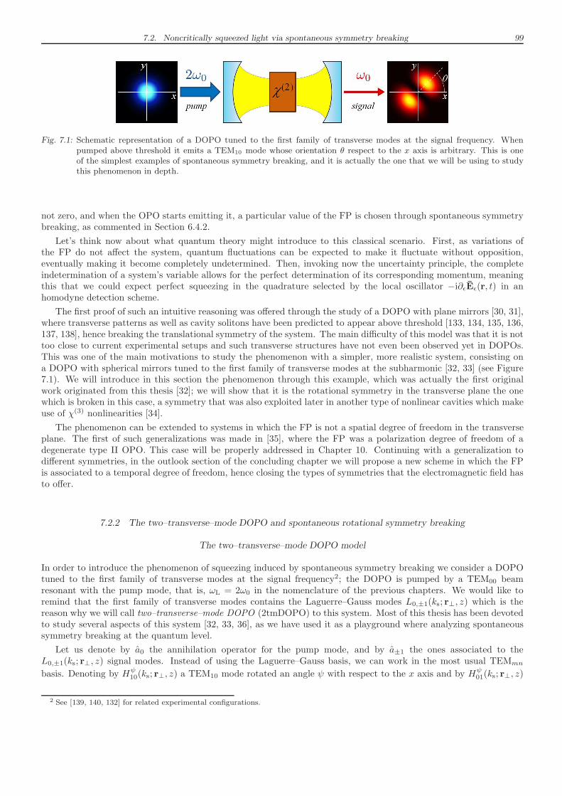
7.2. Noncritically squeezed light via spontaneous symmetry breaking 99

Fig. 7.1: Schematic representation of a DOPO tuned to the first family of transverse modes at the signal frequency. Whenpumped above threshold it emits a TEM10 mode whose orientation θ respect to the x axis is arbitrary. This is oneof the simplest examples of spontaneous symmetry breaking, and it is actually the one that we will be using to studythis phenomenon in depth.

not zero, and when the OPO starts emitting it, a particular value of the FP is chosen through spontaneous symmetrybreaking, as commented in Section 6.4.2.

Let’s think now about what quantum theory might introduce to this classical scenario. First, as variations ofthe FP do not affect the system, quantum fluctuations can be expected to make it fluctuate without opposition,eventually making it become completely undetermined. Then, invoking now the uncertainty principle, the completeindetermination of a system’s variable allows for the perfect determination of its corresponding momentum, meaningthis that we could expect perfect squeezing in the quadrature selected by the local oscillator −i∂ǫEǫ(r, t) in anhomodyne detection scheme.

The first proof of such an intuitive reasoning was offered through the study of a DOPO with plane mirrors [30, 31],where transverse patterns as well as cavity solitons have been predicted to appear above threshold [133, 134, 135, 136,137, 138], hence breaking the translational symmetry of the system. The main difficulty of this model was that it is nottoo close to current experimental setups and such transverse structures have not even been observed yet in DOPOs.This was one of the main motivations to study the phenomenon with a simpler, more realistic system, consisting ona DOPO with spherical mirrors tuned to the first family of transverse modes at the subharmonic [32, 33] (see Figure7.1). We will introduce in this section the phenomenon through this example, which was actually the first originalwork originated from this thesis [32]; we will show that it is the rotational symmetry in the transverse plane the onewhich is broken in this case, a symmetry that was also exploited later in another type of nonlinear cavities which makeuse of χ(3) nonlinearities [34].

The phenomenon can be extended to systems in which the FP is not a spatial degree of freedom in the transverseplane. The first of such generalizations was made in [35], where the FP was a polarization degree of freedom of adegenerate type II OPO. This case will be properly addressed in Chapter 10. Continuing with a generalization todifferent symmetries, in the outlook section of the concluding chapter we will propose a new scheme in which the FPis associated to a temporal degree of freedom, hence closing the types of symmetries that the electromagnetic field hasto offer.

7.2.2 The two–transverse–mode DOPO and spontaneous rotational symmetry breaking

The two–transverse–mode DOPO model

In order to introduce the phenomenon of squeezing induced by spontaneous symmetry breaking we consider a DOPOtuned to the first family of transverse modes at the signal frequency2; the DOPO is pumped by a TEM00 beamresonant with the pump mode, that is, ωL = 2ω0 in the nomenclature of the previous chapters. We would like toremind that the first family of transverse modes contains the Laguerre–Gauss modes L0,±1(ks; r⊥, z) which is thereason why we will call two–transverse–mode DOPO (2tmDOPO) to this system. Most of this thesis has been devotedto study several aspects of this system [32, 33, 36], as we have used it as a playground where analyzing spontaneoussymmetry breaking at the quantum level.

Let us denote by a0 the annihilation operator for the pump mode, and by a±1 the ones associated to theL0,±1(ks; r⊥, z) signal modes. Instead of using the Laguerre–Gauss basis, we can work in the most usual TEMmn

basis. Denoting by Hψ10(ks; r⊥, z) a TEM10 mode rotated an angle ψ with respect to the x axis and by Hψ

01(ks; r⊥, z)

2 See [139, 140, 132] for related experimental configurations.

100 7. Basic phenomena in multi–mode OPOs

to its orthogonal, these are given by

Hψ10(ks; r⊥, z) =

1√2

[

e−iψL0,+1(ks; r⊥, z) + eiψL0,−1(ks; r⊥, z)]

=√2|L0,±1(ks; r⊥, z)| cos(φ− ψ), (7.18a)

Hψ01(ks; r⊥, z) =

1√2i

[

e−iψL0,+1(ks; r⊥, z)− eiψL0,−1(ks; r⊥, z)]

=√2|L0,±1(ks; r⊥, z)| sin(φ− ψ). (7.18b)

These relations can be inverted as

L0,±1(ks; r⊥, z) =1√2e±iψ

[

Hψ10(ks; r⊥, z)± iHψ

01(ks; r⊥, z)]

. (7.19)

The part of the signal field propagating along +ez can be written as (Schrodinger picture is understood)

E(+)s,→ (r) = i

√

~ωs

4ε0nsLsee [a+1L0,+1(ks; r⊥, z) + a−1L0,−1(ks; r⊥, z)] e

insksz, (7.20)

Introducing the relation (7.19) between the Laguerre–Gauss and the Hermite–Gauss modes in this expression, we findthe relation between their corresponding annihilation operators:

a10,ψ =1√2

(

eiψa+1 + e−iψa−1)

, (7.21a)

a01,ψ =i√2

(

eiψa+1 − e−iψa−1)

. (7.21b)

The quantum model for this OPO configuration was already introduced in Section 6.2; we just need to particularizethe three–wave mixing Hamiltonian (6.42) to the case of operating in frequency degenerate type I conditions with onlythe L0,±1(ks; r⊥, z) present at the signal frequency3. Working as usual in a picture rotated to the frequency of theinjected laser, which in this case is described by the operator

U0 = exp[H0t/i~] with H0 = ~ω0(2a†0a0 + a†+1a+1 + a†−1a−1), (7.22)

the master equation of the system can be written in this case as

dρIdt

=[

χa0a†+1a†−1 + Epa†0 +H.c., ρI

]

+∑

j=0,±1

γj(2aj ρIa†j − a

†j aj ρI − ρIa

†j aj), (7.23)

where we will denote γ0 by γp to match our previous notation, and will assume that γ+1 = γ−1 = γs which is as toassume that the DOPO is invariant under rotations around the longitudinal axis, that is, rotationally symmetric inthe transverse plane. As usual, we take Ep as a positive real. On the other hand, the nonlinear coupling parameter χcan be found by particularizing (6.1.2) to the current situation; taking into account that

∫ +∞

0

rdrG(kp; r)[

R10(ks; r)

]2=

(

2

π

)3/2 ∫ +∞

0

dr2r3

wpw4s

exp

[

−(

1

w2p

+2

w2s

)

r2]

=1

4π3/2ws(7.24)

where we have used that w2p/w

2s = λp/λs = 1/2, see (3.86b), we get

χ =3

2

lcwsχ(2)oee(2ω0;ω0, ω0)

√

~ω30

8π3ε0n3cL

3opt

. (7.25)

The above master equation has exactly the same form as that modeling the OPO, see (6.92); this makes perfect sense,as even though the down–converted photons are indistinguishable in frequency and polarization, they are not in orbitalangular momentum, and hence the 2tmDOPO is not a truly degenerate system. From an operational point of viewthis is very fortunate, as we can then directly take the Langevin equations that we already derived for the OPO, and

3 From the previous section we know now that the only important feature is that this process is the one with the highest gain, it doesn’tmatter if other processes are present (such as frequency non-degenerate processes or processes involving other transverse families), as longas these have a higher threshold.

7.2. Noncritically squeezed light via spontaneous symmetry breaking 101

rewrite them to match the notation of the current system. Using also the same scaling for the coherent amplitudes,the time, the noises, and the parameters as in Section 6.4.1, see (6.95) and (6.53), this allows us to write

β0 = κ[σ − β0 − β+1β−1], (7.26a)

β+0 = κ[σ − β+

0 − β++1β

+−1], (7.26b)

β+1 = −β+1 + β0β+−1 + g

√

β0ζ(τ), (7.26c)

β++1 = −β+

+1 + β+0 β−1 + g

√

β+0 ζ

+(τ), (7.26d)

β−1 = −β−1 + β0β++1 + g

√

β0ζ∗(τ), (7.26e)

β+−1 = −β+

−1 + β+0 β+1 + g

√

β+0 [ζ

+(τ)]∗. (7.26f)

Let us finally remind that the squeezing spectrum of any signal mode can be evaluated from this normalized variablesas

S(Xϕm; Ω) =

2

g2

∫ +∞

−∞

dτ ′ exp(−iΩτ ′)〈δxϕm (τ) δxϕm (τ + τ ′)〉P , (7.27)

withxϕm (τ) = e−iϕβm (τ) + eiϕβ+

m (τ) , (7.28)

m referring to any of transverse modes resonating at the signal frequency.

Classical emission: Spontaneous rotational symmetry breaking

We now show that above threshold the two–transverse–mode DOPO shows the phenomenon of spontaneous symmetrybreaking of its rotational invariance in the transverse plane.

Following the approach introduced in the previous chapter, the classical equations of the system are retrieved fromthe Langevin equations by neglecting the noise terms and making the correspondences β+

j → β∗j to come back to theclassical phase space:

β0 = κ[σ − β0 − β+1β−1], (7.29a)

β+1 = −β+1 + β0β∗−1, (7.29b)

β−1 = −β−1 + β0β∗+1. (7.29c)

Now, from our previous treatment of the OPO (see Section 6.4.2) we can directly understand the classical emissionproperties of the current 2tmDOPO. For σ ≤ 1 the signal modes are switched off, that is, its only long time termstable solution is

β0 = σ, β+1 = β−1 = 0. (7.30)

On the other hand, for σ > 1 the only stable solution is

β0 = 1, β±1 = ρ exp(∓iθ), (7.31)

with ρ =√σ − 1 and where θ is arbitrary, as the classical equations are invariant under the change β±1 −→

exp(∓iθ)β±1, that is, θ is the FP of the 2tmDOPO. Taking the expectation value of expression (7.20), and us-ing4 〈a±1(t)〉 = exp(−iω0t)β±1/g within the classical limit, we get the form of the signal field as predicted by classicaloptics

E(+)s,→ (r, t) = i

√

~ωs(σ − 1)

4ε0nsLsg2ee[

e−iθL0,+1(ks; r⊥, z) + eiθL0,−1(ks; r⊥, z)]

e−iω0t+insksz ∝ Hθ10(ks; r⊥, z), (7.33)

that is, classical emission takes place in the form of a TEM10 mode forming an angle θ with respect to the x axis (seeFigure 7.1). Hence, the FP is identified in this case with the orientation of the transverse pattern which is formed abovethreshold, what finally shows that the rotational transverse symmetry of the 2tmDOPO is spontaneously broken.

In the following, we will call bright mode to Hθ10(ks; r⊥, z) —as it is classically excited— and dark mode to its

orthogonal Hθ01(ks; r⊥, z) —as it is classically empty of photons—, and will define the collective indices b = (10, θ)

and d = (01, θ) to simplify the notation.

4 Note that this result comes from the following chain of equalities:

〈a±1(t)〉 = trρIU†0 a±1U0 = exp(−iω0t)trρIa±1 = exp(−iω0t)〈α±1〉P = exp(−iω0t)〈β±1〉P /g (7.32)

102 7. Basic phenomena in multi–mode OPOs

Quantum properties: Pattern diffusion and noncritical squeezing

The linearized Langevin equations. Just as we did with the DOPO, we are going to discuss the quantum propertiesof the down–converted field by inspection of the quantum Langevin equations (7.26) in the limit γp ≫ γs, i.e., κ≫ 1,where the pump variables can be adiabatically eliminated. We will show in the next chapter that all the importantproperties found in this limit are valid in general.

As we already commented in Section 6.3.3, the deterministic procedure for adiabatically eliminating the pumpmodes (which consists in assuming that β0 = β+

0 = 0) is still valid in the stochastic case, but only if the equations areinterpreted in the Ito sense. Hence, after applying this procedure, the Langevin equations read in Stratonovich form:

β+1 = −(

1− g2/4)

β+1 + (σ − β+1β−1)β+−1 + g

√

σ − β+1β−1ζ (τ) , (7.34a)

β++1 = −

(

1− g2/4)

β++1 + (σ − β+

+1β+−1)β−1 + g

√

σ − β++1β

+−1ζ

+ (τ) , (7.34b)

β−1 = −(

1− g2/4)

β−1 + (σ − β+1β−1)β++1 + g

√

σ − β+1β−1ζ∗ (τ) , (7.34c)

β+−1 = −

(

1− g2/4)

β+−1 + (σ − β+

+1β+−1)β+1 + g

√

σ − β++1β

+−1

[

ζ+ (τ)]∗. (7.34d)

In order to find analytic predictions from these equations we are going to linearize them. As explained in theprevious chapter, the usual procedure begins by writing the amplitudes as βm = βm + δβm and β+

m = β∗m + δβ+m,

and treat the fluctuations as order g perturbations. This is in particular how we proceeded with the OPO. However,as already stated in the previous chapter and emphasized in the present one, we expect quantum noise to rotatethe generated TEM10 mode (that is, to make the phase difference between the opposite angular momentum modesdiffuse), and hence fluctuations of the fields in an arbitrary direction of phase space could not be small (i.e., order g).Nevertheless, equations (7.34) can be linearized if the amplitudes are expanded as

β±1 (τ) = [ρ+ b±1 (τ)] e∓iθ(τ) (7.35a)

β+±1 (τ) =

[

ρ+ b+±1 (τ)]

e±iθ(τ), (7.35b)

because as we will prove θ (τ) carries the larger part of the fluctuations, while the b’s and θ remain as order g quantities.In addition, expanding the fields in this way allows us to track the evolution of the classical pattern’s orientation, aswe take θ as an explicit quantum variable. Then, writing equations (7.34) up to order g, we arrive to the followinglinear system (arriving to this expression is not as straightforward as it might seem, there are some subtleties that weclarify in Appendix C)

− 2iiρw0θ + b =Lb+ gζ (τ) , (7.36)

with

b =

b+1

b++1

b−1b+−1

, ζ (τ) =

ζ (τ)ζ+ (τ)ζ∗ (τ)

[ζ+ (τ)]∗

, (7.37)

and where L is a real, symmetric matrix given by

L = −

σ 0 σ − 1 −10 σ −1 σ − 1

σ − 1 −1 σ 0−1 σ − 1 0 σ

, (7.38)

with the following eigensystem

λ0 = 0, w0 = 12 col (1,−1,−1, 1)

λ1 = −2, w1 = 12 col (1, 1,−1,−1)

λ2 = −2 (σ − 1) , w2 = 12 col (1, 1, 1, 1)

λ3 = −2σ, w3 = 12 col (1,−1, 1,−1) .

(7.39)

Defining the projections cm (τ) = wm · b (τ), and projecting the linear system (7.36) onto these eigenmodes, wefind the following set of decoupled linear equations (c0 is set to zero, as otherwise it would just entail a redefinition of

7.2. Noncritically squeezed light via spontaneous symmetry breaking 103

θ)

θ =g

2ρη0 (τ) (7.40a)

c1 = −2c1 + igη1 (τ) (7.40b)

c2 = −2 (σ − 1) c2 + gη2 (τ) (7.40c)

c3 = −2σc3 + gη3 (τ) , (7.40d)

where the following real noises have been defined

η0 (τ) = iw0 · ζ (τ) = Im

ζ+ (τ) − ζ (τ)

(7.41a)

η1 (τ) = −iw1 · ζ (τ) = Im

ζ+ (τ) + ζ (τ)

(7.41b)

η2 (τ) = w2 · ζ (τ) = Re

ζ (τ) + ζ+ (τ)

(7.41c)

η3 (τ) = w3 · ζ (τ) = Re

ζ (τ)− ζ+ (τ)

, (7.41d)

which satisfy the usual statistical properties (2.82).

Note finally that in the long time term the solutions for the projections cj will be of order g (see Appendix B), andhence so will be the b’s (note that this is not the case for θ, whose initial value is completely arbitrary, although itsvariation θ is indeed of order g). This is consistent with the initial assumptions about the orders in g of the involvedquantities.

Quantum diffusion of the classical pattern. Just as we commented in the previous sections, equation (7.40a)shows that the orientation of the bright mode (the FP of the system) diffuses with time ruled by quantum noise. Howfast this diffusion is can be measured by evaluating the variance of θ. Using the statistical properties of noise (2.82),it is straightforward to obtain the following result

Vθ (τ) =⟨

δθ2 (τ)⟩

P= Dτ , (7.42)

where D = d/ (σ − 1) with

d = g2/4 = χ2/4γpγs. (7.43)

Note that we have assumed that Vθ (0) = 0, which is as saying that every time the 2tmDOPO is switched on, thatis, on any stochastic realization, the bright mode appears with the same orientation; in Chapter 9 we will show thatthe pattern can be locked to a desired orientation by injecting a low–power TEM10 seed at the signal frequency insidethe cavity, and hence our assumption can be satisfied experimentally by switching on the 2tmDOPO with this seedpresent, and turning it off at one point so that quantum noise can start making the bright mode rotate arbitrarily.

Passing to quantitative matters, Eq. (7.42) shows that the delocalization of the pattern’s orientation increases astime passes by, though for typical system parameters (see Section 6.3.3, where we argued that g ≈ 4× 10−6) one findsd ≃ 4× 10−12, and hence the rotation of the pattern will be fast only when working extremely close to threshold.

Independent quadratures and noncritical squeezing. The first step towards analyzing the squeezing prop-erties of the field within the framework presented above, is identifying a set of independent quadratures. As showedin the previous analysis, these appear naturally within our approach, as the eigenmodes wmm=0,1,2,3 of the stabilitymatrix give us a set of quadratures with well defined squeezing properties. In particular, from (7.35), (7.21), and(7.28), it is easy to find the following relations

xb (τ) = 2√2ρ+

√2c2 (τ) (7.44a)

yb (τ) = −i√2c3 (τ) (7.44b)

xd (τ) = i√2c0 (τ) (7.44c)

yd (τ) =√2c1 (τ) , (7.44d)

where xb, yb and xd, yd are the (normalized) X and Y quadratures of the bright and dark modes, Hθ10(ks; r⊥, z)

and Hθ01(ks; r⊥, z), respectively.

The evolution of these quadratures can therefore be found from the equations satisfied by the projections (7.40),which are solved in Appendix B (remember that c0 = 0). In particular, using the expression for the correlation

104 7. Basic phenomena in multi–mode OPOs

spectrum of the projections (B.6) as usual, it is straightforward to find the following results

V out(

Xb; Ω)

= 1 +1

(σ − 1)2 + Ω2/4(7.45a)

V out(

Yb; Ω)

= 1− 1

σ2 + Ω2/4(7.45b)

V out(

Xd; Ω)

= 1 (7.45c)

V out(

Yd; Ω)

= 1− 1

1 + Ω2/4. (7.45d)

We see that the quadratures of the bright mode have the same behavior as those of the single mode DOPO: The

quadrature Yb is perfectly squeezed (V out = 0) at zero noise frequency(

Ω = 0)

only at the bifurcation (σ = 1).

On the other hand, the dark mode has perfect squeezing in its Y quadrature at zero noise frequency. What isinteresting is that this result is independent of the distance from threshold, and thus, it is a noncritical phenomenon.

This result was first shown in [32], and we can understand it by following the reasoning given in above: As theorientation θ of the classically excited pattern is undetermined in the long–time limit, its orbital angular momentummust be fully determined at low noise frequencies. On the other hand, the orbital angular momentum of the brightmode Hθ

10(ks; r⊥, z) is nothing but its π/2 phase shifted orthogonal Hermite–Gauss mode, i.e., −i∂φHθ10(ks; r⊥, z =

iHθ01(ks; r⊥, z), which used as a local oscillator in a homodyne detection experiment would lead to the observation of

the Yd quadrature fluctuations.

8. DEEP STUDY OF SPONTANEOUS SYMMETRY BREAKINGTHROUGH THE TWO–TRANSVERSE–MODE DOPO

In the previous chapter we have learned that spontaneous symmetry breaking allows for the obtention of noncriticallysqueezed light in OPOs. We have introduced this phenomenon by studying a particular example, the two–transverse–mode DOPO, in which the rotational invariance in the transverse plane is the symmetry broken by the TEM10 signalfield generated above threshold; the fundamental results at the quantum level have been that (i) this bright patternrotates randomly in the transverse plane owed to quantum noise, and (ii) the dark mode consisting the the TEM10

mode orthogonal to the generated one shows perfect squeezing on its Y quadrature irrespective of the distance tothreshold.

In this chapter (and the next one) we answer some questions that appear naturally after the results of the previouschapter, and which are important both to get a clear understanding of the phenomenon, and to evaluate up to whatpoint it is experimentally observable.

8.1 On canonical pairs and noise transfer

Although the noncritical squeezing of the dark mode coincide with what was intuitively expected after the argumentsgiven in Section 7.2.1, a strange, unexpected result has appeared in (7.45): The quadratures of the dark mode seemto violate the uncertainty principle as V out(Xd; Ω = 0)V out(Yd; Ω = 0) = 0.

Moreover, the noise spectrum of an arbitrary quadrature of the dark mode, which can be written in terms of its Xand Y quadratures as Xϕ

d = Xd cosϕ+ Yd sinϕ, is

V out(

Xϕd ; Ω

)

= 1− sin2 ϕ

1 + Ω2/4, (8.1)

what shows that all the quadratures of the dark mode (except its X quadrature) are squeezed. Thus two orthogonalquadratures cannot form a canonical pair as they satisfy the relation

V out(Xϕd ; Ω)V

out(Y ϕd ; Ω) < 1, (8.2)

in clear violation of the uncertainty principle. This might look surprising, but one needs to keep in mind that thebright and dark modes are not true modes, as their orientation is not a fixed quantity, but a dynamical variable of theproblem1.

The natural question now is: Where does the excess of noise go if it is not transferred from one quadrature to itsorthogonal one? The intuitive answer is that it goes to the pattern orientation, which is actually fully undeterminedin the long term as we showed above (7.42). This section is devoted to prove this statement.

In particular we will prove that two orthogonal quadratures of the dark mode do not form a canonical pair, whilethe orientation θ is the canonical pair of all the squeezed quadratures. One way to prove this would be to evaluatethe commutator between the corresponding quantum operators. However, θ is half the phase difference between theopposite orbital angular momentum modes a±1, whose associated operator has a very difficult expression [141, 142],making the calculation of the needed commutators quite hard. Nevertheless, in [143] we gave evidences of this via asimple procedure based on the close relation between the quantum commutators and the classical Poisson bracketsintroduced in Section A.1, and this is the one we present here.

Let us then come back to a classical description of the system in which a pair of normal variables νm, ν∗mis associated to each mode of the field. The Poisson bracket between two phase space functions f (νm, ν

∗m) and

1 This gives rise to an even more important question: If the modes depend on the system variables, can we actually select them witha local oscillator? One can try to picture a detection scheme using some kind of feed–forward information in which the orientation of thelocal oscillator is locked somehow to the orientation of the bright or dark modes, but it seems highly unlikely. Nevertheless, we show alongthe next sections that this does not destroy the possibility of observing the phenomenon, or even of using it in applications.

106 8. Deep study of spontaneous symmetry breaking through the 2tmDOPO

h (νm, ν∗m) can be rewritten in terms of the normal variables (instead of the position and momenta) as

f, h =∑

m

2

iωm

(

∂f

∂νm

∂h

∂ν∗m− ∂f

∂ν∗m

∂h

∂νm

)

, (8.3)

where the sum covers all the cavity modes, being ωm their corresponding frequencies.As an example, the Poisson bracket between two orthogonal quadratures of a given mode Xm =

√

ωm/2~(νm+ν∗m)

and Ym = −√

ωm/2~i (νm − ν∗m) is found to be

Xm, Ym = 2/~, (8.4)

which is consistent with the quantum commutator [Xm, Ym] = 2i given the correspondence [Xm, Ym] = i~ Xm, Ym.Now, we say that two observables A and B are canonically related when their commutator is not an operator, but

an imaginary number, that is, when [A, B] = iK with K ∈ R, as therefore they satisfy an uncertainty relation of thetype ∆A∆B ≥ K2/4. In an analogous way, given the relation between the commutators and the Poisson brackets,we will say that two classical observables f (νm, ν

∗m) and h (νm, ν

∗m) form a canonical pair if their Poisson bracket is a

real number, that is, f, h ∈ R.In our case, the functions we are interested in are the classical counterparts of the dark mode quadratures, which

using (7.21) with ψ = θ are written in terms of the normal variables of the Laguerre–Gauss modes as

Xϕd = i

√

ωs

4~

[

e−iϕ(

eiθν+1 − e−iθν−1)]

+ c.c., (8.5)

with the orientation given by

θ =1

2iln

(

ν∗+1ν−1

|ν+1||ν−1|

)

, (8.6)

which is just half the phase difference between ν+1 and ν−1.Now, using the definition of the Poisson brackets (8.3) with m = ±1 and after some algebra, it is simple to show

that

Xϕd , Y

ϕd = −

(|ν+1| − |ν−1|)22~ |ν+1| |ν−1|

, (8.7)

and

Xϕd , θ =

exp(−iϕ)4i√~ωs

(|ν+1|+ |ν−1|)√

|ν+1| |ν−1||ν+1|3/2 |ν−1|3/2

+ c.c. (8.8)

On the other hand, in the 2tmDOPO the number of photons with opposite orbital angular momentum is sensiblyequal, that is, |ν+1| ≈ |ν−1|; in particular, the steady state solution of the system above threshold (7.31) states that|ν±1| =

√

2~/ωs|〈a±1〉| =√

2~/ωs|β±1/g| =√

2~/ωsρ/g, and thus the dominant term of the previous Poisson bracketswill be

Xϕd , X

ϕ+π/2d

≈ 0, (8.9)

and

Xϕd , θ ≈ −

g sinϕ√2~ρ

. (8.10)

Hence, at least at the classical level two orthogonal dark quadratures Xϕd and X

ϕ+π/2d do not form a canonical

pair (moreover, they commute), while Xϕd and θ do. This can be seen as an evidence of the same conclusion for the

corresponding quantum operators.

8.2 Homodyne detection with a fixed local oscillator

So far we have considered the situation in which one is able to detect independently the bright and dark modes.However, as shown by Eq. (7.40a), these modes are rotating randomly, what means that a local oscillator fieldfollowing that random rotation should be used in order to detect them separately. This might be a really complicated,if not impossible, task, so we analyze now the more realistic situation in which the local oscillator is matched to theorthogonal orientation of the emerging pattern only at the initial time, remaining then with the same orientationduring the observation time T . We will show that even in this case, and as the rotation of the modes is quite slow(7.42), large levels of noise reduction can be obtained.

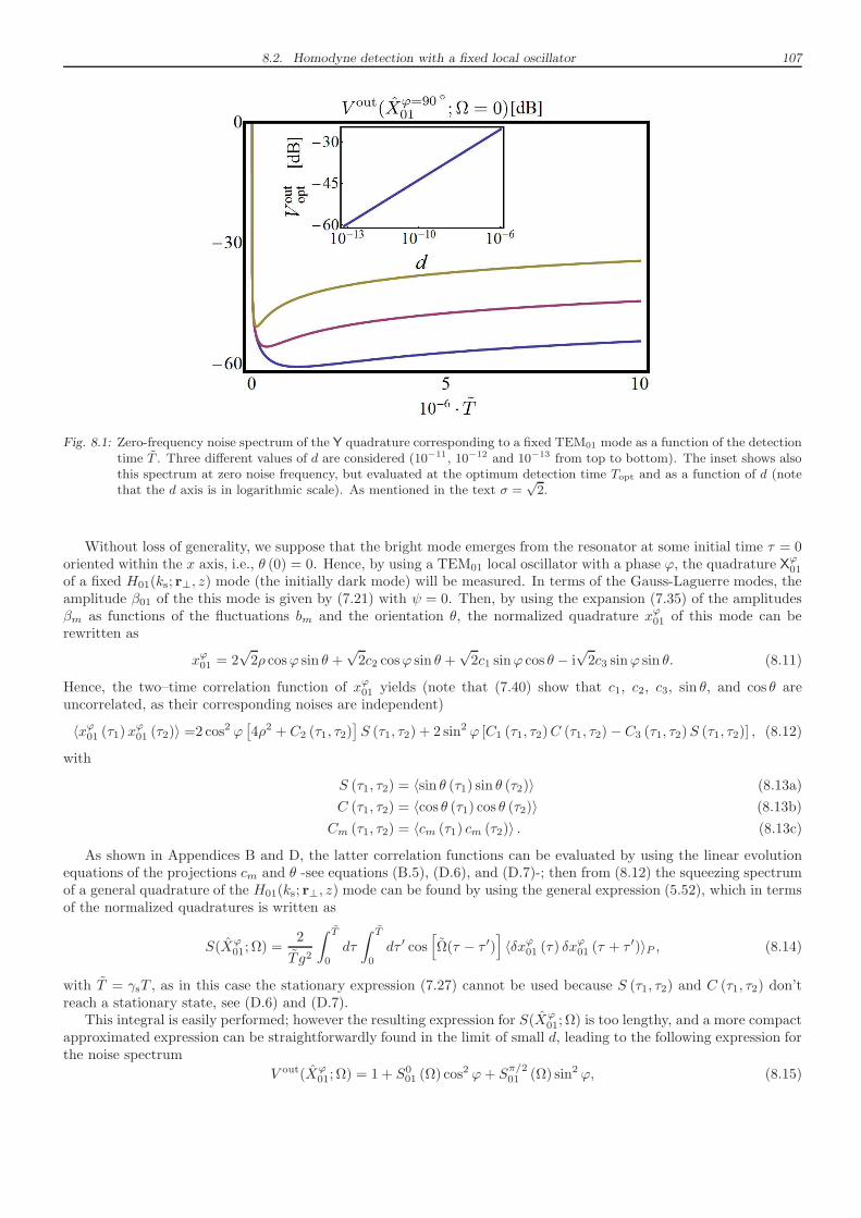
8.2. Homodyne detection with a fixed local oscillator 107

Fig. 8.1: Zero-frequency noise spectrum of the Y quadrature corresponding to a fixed TEM01 mode as a function of the detectiontime T . Three different values of d are considered (10−11, 10−12 and 10−13 from top to bottom). The inset shows alsothis spectrum at zero noise frequency, but evaluated at the optimum detection time Topt and as a function of d (notethat the d axis is in logarithmic scale). As mentioned in the text σ =

√2.

Without loss of generality, we suppose that the bright mode emerges from the resonator at some initial time τ = 0oriented within the x axis, i.e., θ (0) = 0. Hence, by using a TEM01 local oscillator with a phase ϕ, the quadrature Xϕ01of a fixed H01(ks; r⊥, z) mode (the initially dark mode) will be measured. In terms of the Gauss-Laguerre modes, theamplitude β01 of the this mode is given by (7.21) with ψ = 0. Then, by using the expansion (7.35) of the amplitudesβm as functions of the fluctuations bm and the orientation θ, the normalized quadrature xϕ01 of this mode can berewritten as

xϕ01 = 2√2ρ cosϕ sin θ +

√2c2 cosϕ sin θ +

√2c1 sinϕ cos θ − i

√2c3 sinϕ sin θ. (8.11)

Hence, the two–time correlation function of xϕ01 yields (note that (7.40) show that c1, c2, c3, sin θ, and cos θ areuncorrelated, as their corresponding noises are independent)

〈xϕ01 (τ1)xϕ01 (τ2)〉 =2 cos2 ϕ[

4ρ2 + C2 (τ1, τ2)]

S (τ1, τ2) + 2 sin2 ϕ [C1 (τ1, τ2)C (τ1, τ2)− C3 (τ1, τ2)S (τ1, τ2)] , (8.12)

with

S (τ1, τ2) = 〈sin θ (τ1) sin θ (τ2)〉 (8.13a)

C (τ1, τ2) = 〈cos θ (τ1) cos θ (τ2)〉 (8.13b)

Cm (τ1, τ2) = 〈cm (τ1) cm (τ2)〉 . (8.13c)

As shown in Appendices B and D, the latter correlation functions can be evaluated by using the linear evolutionequations of the projections cm and θ -see equations (B.5), (D.6), and (D.7)-; then from (8.12) the squeezing spectrumof a general quadrature of the H01(ks; r⊥, z) mode can be found by using the general expression (5.52), which in termsof the normalized quadratures is written as

S(Xϕ01; Ω) =

2

T g2

∫ T

0

dτ

∫ T

0

dτ ′ cos[

Ω(τ − τ ′)]

〈δxϕ01 (τ) δxϕ01 (τ + τ ′)〉P , (8.14)

with T = γsT , as in this case the stationary expression (7.27) cannot be used because S (τ1, τ2) and C (τ1, τ2) don’treach a stationary state, see (D.6) and (D.7).

This integral is easily performed; however the resulting expression for S(Xϕ01; Ω) is too lengthy, and a more compact

approximated expression can be straightforwardly found in the limit of small d, leading to the following expression forthe noise spectrum

V out(Xϕ01; Ω) = 1 + S0

01 (Ω) cos2 ϕ+ S

π/201 (Ω) sin2 ϕ, (8.15)

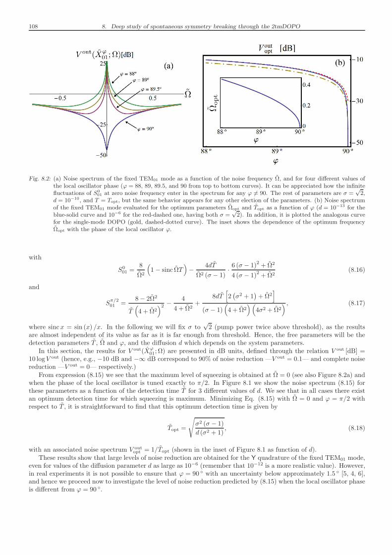
108 8. Deep study of spontaneous symmetry breaking through the 2tmDOPO

Fig. 8.2: (a) Noise spectrum of the fixed TEM01 mode as a function of the noise frequency Ω, and for four different values ofthe local oscillator phase (ϕ = 88, 89, 89.5, and 90 from top to bottom curves). It can be appreciated how the infinitefluctuations of S0

01 at zero noise frequency enter in the spectrum for any ϕ 6= 90. The rest of parameters are σ =√2,

d = 10−10, and T = Topt, but the same behavior appears for any other election of the parameters. (b) Noise spectrumof the fixed TEM01 mode evaluated for the optimum parameters Ωopt and Topt as a function of ϕ (d = 10−13 for theblue-solid curve and 10−6 for the red-dashed one, having both σ =

√2). In addition, it is plotted the analogous curve

for the single-mode DOPO (gold, dashed-dotted curve). The inset shows the dependence of the optimum frequencyΩopt with the phase of the local oscillator ϕ.

with

S001 =

8

Ω2

(

1− sinc ΩT)

− 4dT

Ω2 (σ − 1)· 6 (σ − 1)2 + Ω2

4 (σ − 1)2+ Ω2

(8.16)

and

Sπ/201 =

8− 2Ω2

T(

4 + Ω2)2 −

4

4 + Ω2+

8dT[

2(

σ2 + 1)

+ Ω2]

(σ − 1)(

4 + Ω2)(

4σ2 + Ω2) , (8.17)

where sincx = sin (x) /x. In the following we will fix σ to√2 (pump power twice above threshold), as the results

are almost independent of its value as far as it is far enough from threshold. Hence, the free parameters will be thedetection parameters T , Ω and ϕ, and the diffusion d which depends on the system parameters.

In this section, the results for V out(Xϕ01; Ω) are presented in dB units, defined through the relation V out [dB] =

10 logV out (hence, e.g., −10 dB and −∞ dB correspond to 90% of noise reduction —V out = 0.1— and complete noisereduction —V out = 0— respectively.)

From expression (8.15) we see that the maximum level of squeezing is obtained at Ω = 0 (see also Figure 8.2a) andwhen the phase of the local oscillator is tuned exactly to π/2. In Figure 8.1 we show the noise spectrum (8.15) forthese parameters as a function of the detection time T for 3 different values of d. We see that in all cases there existan optimum detection time for which squeezing is maximum. Minimizing Eq. (8.15) with Ω = 0 and ϕ = π/2 withrespect to T , it is straightforward to find that this optimum detection time is given by

Topt =

√

σ2 (σ − 1)

d (σ2 + 1), (8.18)

with an associated noise spectrum V outopt = 1/Topt (shown in the inset of Figure 8.1 as function of d).

These results show that large levels of noise reduction are obtained for the Y quadrature of the fixed TEM01 mode,even for values of the diffusion parameter d as large as 10−6 (remember that 10−12 is a more realistic value). However,in real experiments it is not possible to ensure that ϕ = 90 with an uncertainty below approximately 1.5 [5, 4, 6],and hence we proceed now to investigate the level of noise reduction predicted by (8.15) when the local oscillator phaseis different from ϕ = 90 .

8.3. Beyond the considered approximations 109

Of course, when ϕ 6= 90 the noise frequency with maximum squeezing is no longer Ω = 0, as in this case theinfinite fluctuations of S0

01 at zero noise frequency, due to the rotation noise, enter the noise spectrum (see Figure8.2a). By numerical minimization of V out(Xϕ

01; Ω) with respect to Ω and T for different values of ϕ and d, it is possibleto show that the optimum value of the detection time is almost independent of ϕ for small deviations of this from 90 ,and hence it is still given to a good approximation by (8.18), although in this case this minimum is less pronouncedthan in the ϕ = 90 case shown in Figure 8.1 (i.e., the curve is almost horizontal around Topt). On the other hand,

the optimum noise frequency Ωopt is independent of d and depends on ϕ as shown in the inset of Figure 8.2b.

As for the squeezing level, in Figure 8.2b we show the noise spectrum evaluated at Topt and Ωopt as a functionof ϕ for 2 different values of the diffusion d. Together with these curves, we have plotted the noise spectrum of thesingle–mode DOPO2 evaluated for its optimum parameters (in this case it is optimized respect to σ and Ω) as afunction of ϕ. We see that the noise reduction is independent of d as ϕ is taken apart from 90 . On the other hand,the squeezing level is similar to that of the single–mode DOPO, as the maximum difference between them are 1.5 dB(a factor 1.4 in the noise spectrum) in favor of the single–mode DOPO, with the advantage that in the 2tmDOPOthis level is independent of the distance from threshold.

Therefore we see that the phenomenon of noncritical squeezing through spontaneous rotational symmetry breakingcould be observed in the 2tmDOPO without the need of following the random rotation of the generated pattern, whichmakes its experimental realization feasible with currently available technology.

8.3 Beyond the considered approximations

8.3.1 Beyond the adiabatic elimination of the pump

The first assumption made in the search for the quantum properties of the system was that γp ≫ γs, a limit thatallowed the adiabatic elimination of the pump field. Now we are going to show analytically that the phenomenon ofsqueezing induced by spontaneous rotational symmetry breaking is still present even without this assumption, but stillworking within the linearized theory (in the next section we will check it via a numerical simulation of the completenonlinear stochastic equations).

The way to show this is quite simple; starting from the complete equations (7.26), we expand the amplitudes βmaround the classical stationary solution (7.31) as we made in (7.35), but adding now a similar expression for the pumpamplitudes: β0 = 1 + b0 and β+

0 = 1 + b+0 (note that for the pump modes the b’s are directly small as the phase ofthis mode is locked to that of the injection Ep). Then, linearizing these equations for the fluctuations and noises, wearrive to a linear system formally equal to (7.36), but with

b =

b0b+0b+1

b++1

b−1b+−1

, ζ =

00

ζ (τ)ζ+ (τ)ζ∗ (τ)

[ζ+ (τ)]∗

, (8.19)

and a linear matrix

L =

−κ 0 −ρ 0 −ρ 00 −κ 0 −ρ 0 −ρρ 0 −1 0 0 10 ρ 0 −1 1 0ρ 0 0 1 −1 00 ρ 1 0 0 −1

. (8.20)

Although in this case L is not Hermitian, it can be checked that it possess a biorthonormal eigenbasis3, andin particular, the following two vectors are present in its eigensystem: w′0 = 1

2 col (0, 0, 1,−1,−1, 1) and w′1 =12 col (0, 0, 1, 1,−1,−1), with corresponding eigenvalues λ′0 = 0 and λ′1 = −2. These eigenvectors have null projec-tion onto the pump subspace, and coincide with w0 and w1 in what concerns to the signal subspace, see (7.39).Hence, all the properties derived from these vectors are still present without any change. In particular, as they ac-count for the diffusion of θ and the squeezing properties of the dark mode, we can conclude that these properties arestill present when working out of the limit γp ≫ γs.

2 In the single–mode DOPO the best levels of squeezing are found below threshold, where its noise spectrum can be written as

V out(

Xϕs ; Ω

)

= 1 + S+ (Ω) cos2 ϕ− S− (Ω) sin2 ϕ, with S± (Ω) = 4σ/[

(σ ± 1)2 + Ω2]

, see (6.76).3 This means that there exist a set of eigenvectors vm satisfying Lvm = λmvm, and another set wm satisfying L†wm = λ∗mwm, such

that w∗m · vm = δmn.

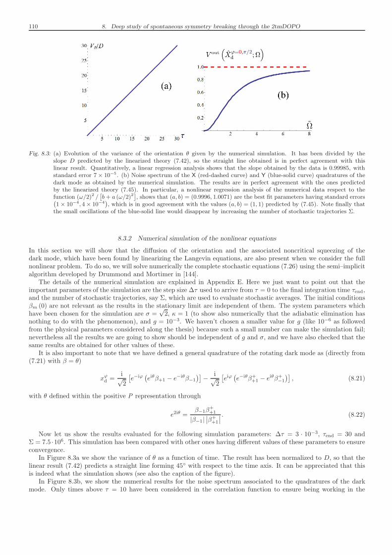
110 8. Deep study of spontaneous symmetry breaking through the 2tmDOPO

Fig. 8.3: (a) Evolution of the variance of the orientation θ given by the numerical simulation. It has been divided by theslope D predicted by the linearized theory (7.42), so the straight line obtained is in perfect agreement with thislinear result. Quantitatively, a linear regression analysis shows that the slope obtained by the data is 0.99985, withstandard error 7× 10−5. (b) Noise spectrum of the X (red-dashed curve) and Y (blue-solid curve) quadratures of thedark mode as obtained by the numerical simulation. The results are in perfect agreement with the ones predictedby the linearized theory (7.45). In particular, a nonlinear regression analysis of the numerical data respect to thefunction (ω/2)2 /

[

b+ a (ω/2)2]

, shows that (a, b) = (0.9996, 1.0071) are the best fit parameters having standard errors(

1× 10−4, 4× 10−4)

, which is in good agreement with the values (a, b) = (1, 1) predicted by (7.45). Note finally thatthe small oscillations of the blue-solid line would disappear by increasing the number of stochastic trajectories Σ.

8.3.2 Numerical simulation of the nonlinear equations

In this section we will show that the diffusion of the orientation and the associated noncritical squeezing of thedark mode, which have been found by linearizing the Langevin equations, are also present when we consider the fullnonlinear problem. To do so, we will solve numerically the complete stochastic equations (7.26) using the semi–implicitalgorithm developed by Drummond and Mortimer in [144].

The details of the numerical simulation are explained in Appendix E. Here we just want to point out that theimportant parameters of the simulation are the step size ∆τ used to arrive from τ = 0 to the final integration time τend,and the number of stochastic trajectories, say Σ, which are used to evaluate stochastic averages. The initial conditionsβm (0) are not relevant as the results in the stationary limit are independent of them. The system parameters whichhave been chosen for the simulation are σ =

√2, κ = 1 (to show also numerically that the adiabatic elimination has

nothing to do with the phenomenon), and g = 10−3. We haven’t chosen a smaller value for g (like 10−6 as followedfrom the physical parameters considered along the thesis) because such a small number can make the simulation fail;nevertheless all the results we are going to show should be independent of g and σ, and we have also checked that thesame results are obtained for other values of these.

It is also important to note that we have defined a general quadrature of the rotating dark mode as (directly from(7.21) with β = θ)

xϕd =i√2

[

e−iϕ(

eiθβ+1 − e−iθβ−1)]

− i√2

[

eiϕ(

e−iθβ++1 − eiθβ+

−1

)]

, (8.21)

with θ defined within the positive P representation through

e2iθ =β−1β

++1

|β−1|∣

∣β++1

∣

∣

. (8.22)

Now let us show the results evaluated for the following simulation parameters: ∆τ = 3 · 10−3, τend = 30 andΣ = 7.5 ·106. This simulation has been compared with other ones having different values of these parameters to ensureconvergence.

In Figure 8.3a we show the variance of θ as a function of time. The result has been normalized to D, so that thelinear result (7.42) predicts a straight line forming 45 with respect to the time axis. It can be appreciated that thisis indeed what the simulation shows (see also the caption of the figure).

In Figure 8.3b, we show the numerical results for the noise spectrum associated to the quadratures of the darkmode. Only times above τ = 10 have been considered in the correlation function to ensure being working in the

8.3. Beyond the considered approximations 111

stationary limit. Again, the results shown in Figure 8.3b are in reasonable agreement with the linear predictions(7.45c) and (7.45d), as explained quantitatively in the caption of Figure 8.3.

These results show that the phenomenon of noncritically squeezed light via spontaneous rotational symmetrybreaking is not a product of the linearization.

112 8. Deep study of spontaneous symmetry breaking through the 2tmDOPO

9. THE TWO–TRANSVERSE–MODE DOPO WITH INJECTED SIGNAL

In this chapter we keep studying the properties of the 2tmDOPO, analyzing in particular how the injection of a TEM10

mode at the signal frequency modifies its properties [36]. The study of this signal seed is motivated by two experimentalissues. First, the arbitrariness of the initial orientation of the above–threshold pattern is highly inconvenient, sinceone cannot know in advance within which orientation it will rise at a particular realization of the experiment, whatmakes the matching of the local oscillator to the initial dark mode quite difficult; hence some means of fixing thisorientation is called for, and we will show that this is exactly what the signal seed accomplishes. On the other hand,it is customary to inject a low intensity signal field in experiments to keep the cavity stable and locked to the desiredfrequency.

Note that this signal seed would break the rotational invariance of the system and hence a degradation of thesqueezing level is expected. The goal of this chapter is then to determine the impact of the signal injection on thequantum properties of the 2tmDOPO.

In what follows, we will refer to this configuration as driven 2tmDOPO, denoting then by free–running 2tmDOPOthe system without the injection at the signal frequency.

We will show that, fortunately, the 2tmDOPO still exhibits large levels of noncritical squeezing, even larger thanthose exhibited by the usual single-mode DOPO with injected signal, a result that is connected with the squeezingdue to the spontaneous breaking of the rotational symmetry that exists in the absence of injection, but also to theexistence of a new bifurcation in the system.

The current system is closely related to that analyzed by Protsenko et al. [145] who considered a single–modeDOPO with injected signal (see also [146, 147]). Indeed our model contains, as a limit, the model studied in [145],but we shall see that the existence of a second signal mode substantially modifies the properties of the system.

9.1 Model of the 2tmDOPO with injected signal

The system we are dealing with is exactly the same as the one we have already studied, with the exception that nowthe signal modes have also an injection term. In the previous chapters we wrote the system’s equations in terms of theLaguerre–Gauss modes; now, however, it is quite recommendable to work in Hermite–Gauss basis, as we are injectingone of these modes. To this aim, we first use the relations (7.21) between the Laguerre–Gauss and the Hermite–Gaussboson operators to write the following relation between the corresponding normalized coherent amplitudes:

β±1 = (βx ∓ iβy) /√2, (9.1)

where βx/y are the coherent amplitudes associated to the H10/01(ks; r⊥, z) modes; then, we use these relations torewrite the Langevin equations (7.26) which model the 2tmDOPO in terms of the βx/y amplitudes, arriving to

β0 = κ[

σ − β0 −(

β2x + β2

y

)

/2]

, (9.2a)

β+0 = κ

[

σ − β+0 −

(

β+2x + β+2

y

)

/2]

, (9.2b)

βx = εi − βx + β0β+x + g

√

β0ζx (τ) , (9.2c)

β+x = ε∗i − β+

x + β+0 βx + g

√

β+0 ζ

+x (τ) , (9.2d)

βy = −βy + β0β+y + g

√

β0ζy (τ) , (9.2e)

β+y = −β+

y + β+0 βy + g

√

β+0 ζ

+y (τ) , (9.2f)

where in addition to the usual dimensionless parameters, we have introduced the normalized injection parameter forthe signal TEM10 mode

εi =χEs

γs√γpγs

, (9.3)

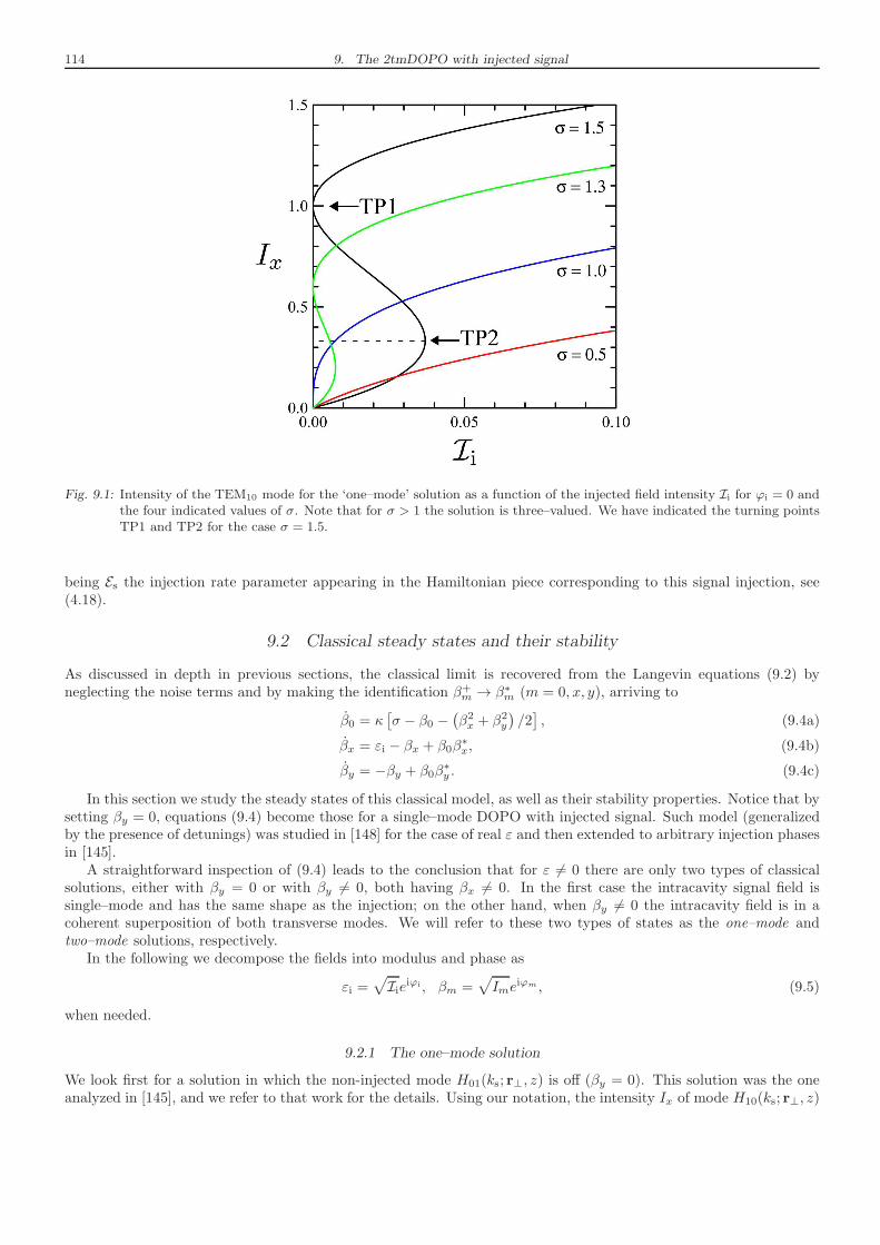
114 9. The 2tmDOPO with injected signal

Fig. 9.1: Intensity of the TEM10 mode for the ‘one–mode’ solution as a function of the injected field intensity Ii for ϕi = 0 andthe four indicated values of σ. Note that for σ > 1 the solution is three–valued. We have indicated the turning pointsTP1 and TP2 for the case σ = 1.5.

being Es the injection rate parameter appearing in the Hamiltonian piece corresponding to this signal injection, see(4.18).

9.2 Classical steady states and their stability

As discussed in depth in previous sections, the classical limit is recovered from the Langevin equations (9.2) byneglecting the noise terms and by making the identification β+

m → β∗m (m = 0, x, y), arriving to

β0 = κ[

σ − β0 −(

β2x + β2

y

)

/2]

, (9.4a)

βx = εi − βx + β0β∗x, (9.4b)

βy = −βy + β0β∗y . (9.4c)

In this section we study the steady states of this classical model, as well as their stability properties. Notice that bysetting βy = 0, equations (9.4) become those for a single–mode DOPO with injected signal. Such model (generalizedby the presence of detunings) was studied in [148] for the case of real ε and then extended to arbitrary injection phasesin [145].

A straightforward inspection of (9.4) leads to the conclusion that for ε 6= 0 there are only two types of classicalsolutions, either with βy = 0 or with βy 6= 0, both having βx 6= 0. In the first case the intracavity signal field issingle–mode and has the same shape as the injection; on the other hand, when βy 6= 0 the intracavity field is in acoherent superposition of both transverse modes. We will refer to these two types of states as the one–mode andtwo–mode solutions, respectively.

In the following we decompose the fields into modulus and phase as

εi =√

Iieiϕi , βm =√

Imeiϕm , (9.5)

when needed.

9.2.1 The one–mode solution

We look first for a solution in which the non-injected mode H01(ks; r⊥, z) is off (βy = 0). This solution was the oneanalyzed in [145], and we refer to that work for the details. Using our notation, the intensity Ix of mode H10(ks; r⊥, z)

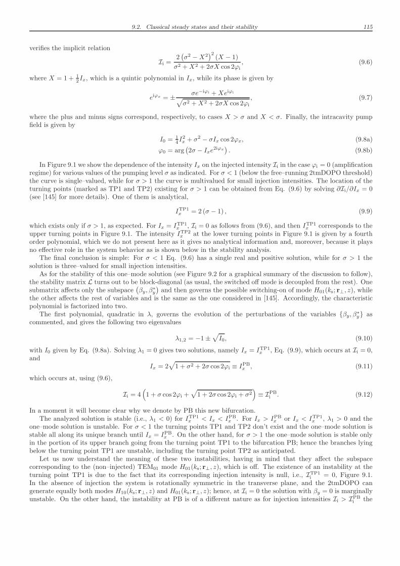
9.2. Classical steady states and their stability 115

verifies the implicit relation

Ii =2(

σ2 −X2)2

(X − 1)

σ2 +X2 + 2σX cos 2ϕi, (9.6)

where X = 1 + 12Ix, which is a quintic polynomial in Ix, while its phase is given by

eiϕx = ± σe−iϕi +Xeiϕi

√

σ2 +X2 + 2σX cos 2ϕi

, (9.7)

where the plus and minus signs correspond, respectively, to cases X > σ and X < σ. Finally, the intracavity pumpfield is given by

I0 = 14I

2x + σ2 − σIx cos 2ϕx, (9.8a)

ϕ0 = arg(

2σ − Ixe2iϕx)

. (9.8b)

In Figure 9.1 we show the dependence of the intensity Ix on the injected intensity Ii in the case ϕi = 0 (amplificationregime) for various values of the pumping level σ as indicated. For σ < 1 (below the free–running 2tmDOPO threshold)the curve is single–valued, while for σ > 1 the curve is multivalued for small injection intensities. The location of theturning points (marked as TP1 and TP2) existing for σ > 1 can be obtained from Eq. (9.6) by solving ∂Ii/∂Ix = 0(see [145] for more details). One of them is analytical,

ITP1x = 2 (σ − 1) , (9.9)

which exists only if σ > 1, as expected. For Ix = ITP1x , Ii = 0 as follows from (9.6), and then ITP1

x corresponds to theupper turning points in Figure 9.1. The intensity ITP2

x at the lower turning points in Figure 9.1 is given by a fourthorder polynomial, which we do not present here as it gives no analytical information and, moreover, because it playsno effective role in the system behavior as is shown below in the stability analysis.

The final conclusion is simple: For σ < 1 Eq. (9.6) has a single real and positive solution, while for σ > 1 thesolution is three–valued for small injection intensities.

As for the stability of this one–mode solution (see Figure 9.2 for a graphical summary of the discussion to follow),the stability matrix L turns out to be block-diagonal (as usual, the switched off mode is decoupled from the rest). Onesubmatrix affects only the subspace

(

βy, β∗y

)

and then governs the possible switching-on of mode H01(ks; r⊥, z), whilethe other affects the rest of variables and is the same as the one considered in [145]. Accordingly, the characteristicpolynomial is factorized into two.

The first polynomial, quadratic in λ, governs the evolution of the perturbations of the variables βy, β∗y ascommented, and gives the following two eigenvalues

λ1,2 = −1±√

I0, (9.10)

with I0 given by Eq. (9.8a). Solving λ1 = 0 gives two solutions, namely Ix = ITP1x , Eq. (9.9), which occurs at Ii = 0,

andIx = 2

√

1 + σ2 + 2σ cos 2ϕi ≡ IPBx , (9.11)

which occurs at, using (9.6),

Ii = 4(

1 + σ cos 2ϕi +√

1 + 2σ cos 2ϕi + σ2)

≡ IPBi . (9.12)

In a moment it will become clear why we denote by PB this new bifurcation.The analyzed solution is stable (i.e., λ1 < 0) for ITP1

x < Ix < IPBx . For Ix > IPB

x or Ix < ITP1x , λ1 > 0 and the

one–mode solution is unstable. For σ < 1 the turning points TP1 and TP2 don’t exist and the one–mode solution isstable all along its unique branch until Ix = IPB

x . On the other hand, for σ > 1 the one–mode solution is stable onlyin the portion of its upper branch going from the turning point TP1 to the bifurcation PB; hence the branches lyingbelow the turning point TP1 are unstable, including the turning point TP2 as anticipated.

Let us now understand the meaning of these two instabilities, having in mind that they affect the subspacecorresponding to the (non–injected) TEM01 mode H01(ks; r⊥, z), which is off. The existence of an instability at theturning point TP1 is due to the fact that its corresponding injection intensity is null, i.e., ITP1

i = 0, Figure 9.1.In the absence of injection the system is rotationally symmetric in the transverse plane, and the 2tmDOPO cangenerate equally both modes H10(ks; r⊥, z) and H01(ks; r⊥, z); hence, at Ii = 0 the solution with βy = 0 is marginallyunstable. On the other hand, the instability at PB is of a different nature as for injection intensities Ii > IPB

i the

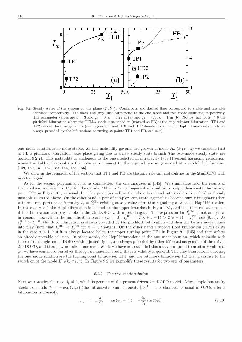
116 9. The 2tmDOPO with injected signal

Fig. 9.2: Steady states of the system on the plane 〈Ii, I10〉. Continuous and dashed lines correspond to stable and unstablesolutions, respectively. The black and grey lines correspond to the one–mode and two–mode solutions, respectively.The parameter values are σ = 3 and ϕi = 0, κ = 0.25 in (a) and ϕi = π/3, κ = 1 in (b). Notice that for Ii 6= 0 thepitchfork bifurcation where the TEM01 mode is switched on (marked as PB) is the only relevant bifurcation. TP1 andTP2 denote the turning points (see Figure 9.1) and HB1 and HB2 denote two different Hopf bifurcations (which arealways preceded by the bifurcations occurring at points TP1 and PB, see text).

one–mode solution is no more stable. As this instability governs the growth of mode H01(ks; r⊥, z) we conclude thatat PB a pitchfork bifurcation takes place giving rise to a new steady state branch (the two–mode steady state, seeSection 9.2.2). This instability is analogous to the one predicted in intracavity type II second harmonic generation,where the field orthogonal (in the polarization sense) to the injected one is generated at a pitchfork bifurcation[149, 150, 151, 152, 153, 154, 155, 156].

We show in the reminder of the section that TP1 and PB are the only relevant instabilities in the 2tmDOPO withinjected signal.

As for the second polynomial it is, as commented, the one analyzed in [145]. We summarize next the results ofthat analysis and refer to [145] for the details. When σ > 1 an eigenvalue is null in correspondence with the turningpoint TP2 in Figure 9.1, as usual, but this point (as well as the whole lower and intermediate branches) is alreadyunstable as stated above. On the other hand, a pair of complex–conjugate eigenvalues become purely imaginary (thenwith null real part) at an intensity Ix = IHB1

x existing at any value of σ, thus signalling a so-called Hopf bifurcation.In the case σ > 1 the Hopf bifurcation is located on the upper branches in Figure 9.1, and it is then relevant to askif this bifurcation can play a role in the 2tmDOPO with injected signal. The expression for IHB1

x is not analyticalin general; however in the amplification regime (ϕi = 0), IHB1

x = 2 (κ+ σ + 1) > 2 (σ + 1) = IPBx , see (9.11). As

IHB1x > IPB1

x , the Hopf bifurcation is always preceded by the pitchfork bifurcation and then the former never comesinto play (note that IHB1

x → IPB1x for κ → 0 though). On the other hand a second Hopf bifurcation (HB2) exists

in the case σ > 1, but it is always located below the upper turning point TP1 in Figure 9.1 [145] and then affectsan already unstable solution. In other words, the Hopf bifurcations of the one–mode solution, which coincide withthose of the single–mode DOPO with injected signal, are always preceded by other bifurcations genuine of the driven2tmDOPO, and then play no role in our case. While we have not extended this analytical proof to arbitrary values ofϕi, we have convinced ourselves through a numerical study, that its validity is general: The only bifurcations affectingthe one–mode solution are the turning point bifurcation TP1, and the pitchfork bifurcation PB that gives rise to theswitch on of the mode H01(ks; r⊥, z). In Figure 9.2 we exemplify these results for two sets of parameters.

9.2.2 The two–mode solution

Next we consider the case βy 6= 0, which is genuine of the present driven 2tmDOPO model. After simple but tricky

algebra on finds β0 = − exp (2iϕi) (the intracavity pump intensity |β0|2 = 1 is clamped as usual in OPOs after abifurcation is crossed),

ϕy = ϕi ±π

2, tan (ϕx − ϕi) = −

4σ

Iisin (2ϕi) , (9.13)

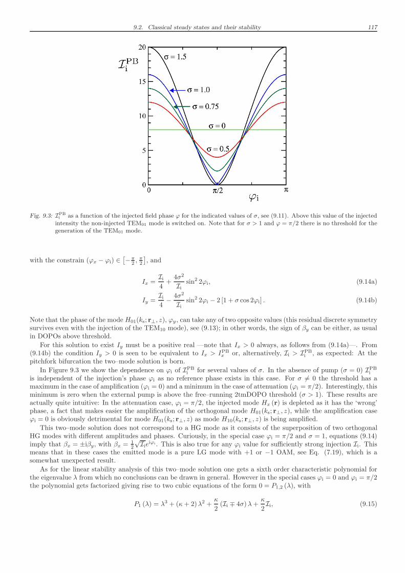
9.2. Classical steady states and their stability 117

Fig. 9.3: IPBi as a function of the injected field phase ϕ for the indicated values of σ, see (9.11). Above this value of the injected

intensity the non-injected TEM01 mode is switched on. Note that for σ > 1 and ϕ = π/2 there is no threshold for thegeneration of the TEM01 mode.

with the constrain (ϕx − ϕi) ∈[

−π2 , π2]

, and

Ix =Ii4+

4σ2

Iisin2 2ϕi, (9.14a)

Iy =Ii4− 4σ2

Iisin2 2ϕi − 2 [1 + σ cos 2ϕi] . (9.14b)

Note that the phase of the mode H01(ks; r⊥, z), ϕy , can take any of two opposite values (this residual discrete symmetrysurvives even with the injection of the TEM10 mode), see (9.13); in other words, the sign of βy can be either, as usualin DOPOs above threshold.

For this solution to exist Iy must be a positive real —note that Ix > 0 always, as follows from (9.14a)—. From(9.14b) the condition Iy > 0 is seen to be equivalent to Ix > IPB

x or, alternatively, Ii > IPBi , as expected: At the

pitchfork bifurcation the two–mode solution is born.

In Figure 9.3 we show the dependence on ϕi of IPBi for several values of σ. In the absence of pump (σ = 0) IPB

i

is independent of the injection’s phase ϕi as no reference phase exists in this case. For σ 6= 0 the threshold has amaximum in the case of amplification (ϕi = 0) and a minimum in the case of attenuation (ϕi = π/2). Interestingly, thisminimum is zero when the external pump is above the free–running 2tmDOPO threshold (σ > 1). These results areactually quite intuitive: In the attenuation case, ϕi = π/2, the injected mode Hx (r) is depleted as it has the ‘wrong’phase, a fact that makes easier the amplification of the orthogonal mode H01(ks; r⊥, z), while the amplification caseϕi = 0 is obviously detrimental for mode H01(ks; r⊥, z) as mode H10(ks; r⊥, z) is being amplified.

This two–mode solution does not correspond to a HG mode as it consists of the superposition of two orthogonalHG modes with different amplitudes and phases. Curiously, in the special case ϕi = π/2 and σ = 1, equations (9.14)imply that βx = ±iβy, with βx = 1

2

√Iieiϕi . This is also true for any ϕi value for sufficiently strong injection Ii. This

means that in these cases the emitted mode is a pure LG mode with +1 or −1 OAM, see Eq. (7.19), which is asomewhat unexpected result.

As for the linear stability analysis of this two–mode solution one gets a sixth order characteristic polynomial forthe eigenvalue λ from which no conclusions can be drawn in general. However in the special cases ϕi = 0 and ϕi = π/2the polynomial gets factorized giving rise to two cubic equations of the form 0 = P1,2 (λ), with

P1 (λ) = λ3 + (κ+ 2)λ2 +κ

2(Ii ∓ 4σ)λ+

κ

2Ii, (9.15)

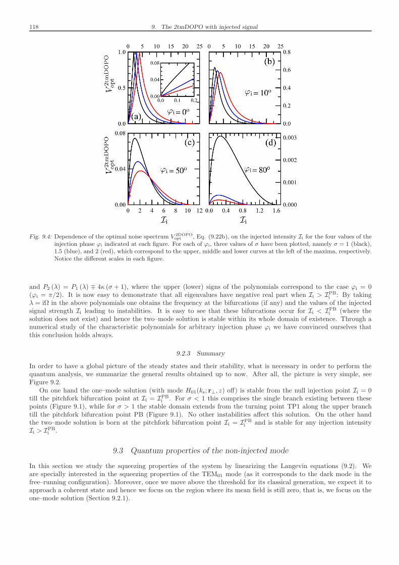
118 9. The 2tmDOPO with injected signal

Fig. 9.4: Dependence of the optimal noise spectrum V 2DOPOopt , Eq. (9.22b), on the injected intensity Ii for the four values of the

injection phase ϕi indicated at each figure. For each of ϕi, three values of σ have been plotted, namely σ = 1 (black),1.5 (blue), and 2 (red), which correspond to the upper, middle and lower curves at the left of the maxima, respectively.Notice the different scales in each figure.

and P2 (λ) = P1 (λ) ∓ 4κ (σ + 1), where the upper (lower) signs of the polynomials correspond to the case ϕi = 0(ϕi = π/2). It is now easy to demonstrate that all eigenvalues have negative real part when Ii > IPB

i : By takingλ = iΩ in the above polynomials one obtains the frequency at the bifurcations (if any) and the values of the injectedsignal strength Ii leading to instabilities. It is easy to see that these bifurcations occur for Ii < IPB

i (where thesolution does not exist) and hence the two–mode solution is stable within its whole domain of existence. Through anumerical study of the characteristic polynomials for arbitrary injection phase ϕi we have convinced ourselves thatthis conclusion holds always.

9.2.3 Summary

In order to have a global picture of the steady states and their stability, what is necessary in order to perform thequantum analysis, we summarize the general results obtained up to now. After all, the picture is very simple, seeFigure 9.2.

On one hand the one–mode solution (with mode H01(ks; r⊥, z) off) is stable from the null injection point Ii = 0till the pitchfork bifurcation point at Ii = IPB

i . For σ < 1 this comprises the single branch existing between thesepoints (Figure 9.1), while for σ > 1 the stable domain extends from the turning point TP1 along the upper branchtill the pitchfork bifurcation point PB (Figure 9.1). No other instabilities affect this solution. On the other handthe two–mode solution is born at the pitchfork bifurcation point Ii = IPB

i and is stable for any injection intensityIi > IPB

i .

9.3 Quantum properties of the non-injected mode

In this section we study the squeezing properties of the system by linearizing the Langevin equations (9.2). Weare specially interested in the squeezing properties of the TEM01 mode (as it corresponds to the dark mode in thefree–running configuration). Moreover, once we move above the threshold for its classical generation, we expect it toapproach a coherent state and hence we focus on the region where its mean field is still zero, that is, we focus on theone–mode solution (Section 9.2.1).

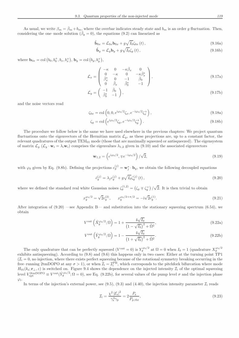
9.3. Quantum properties of the non-injected mode 119

As usual, we write βm = βm+ bm, where the overbar indicates steady state and bm is an order g fluctuation. Then,considering the one–mode solution (βy = 0), the equations (9.2) can linearized as

b0x = L0xb0x + g√

I0ζ0x (t) , (9.16a)

by = Lyby + g√

I0ζy (t) , (9.16b)

where b0x = col(

b0, b+0 , bx, b

+x

)

, by = col(

by, b+y

)

,

Lx =

−κ 0 −κβx 00 −κ 0 −κβ∗xβ∗x 0 −1 β00 βx β∗0 −1

, (9.17a)

Ly =

(

−1 β0β∗0 −1

)

, (9.17b)

and the noise vectors read

ζ0x = col(

0, 0, eiϕ0/2ζx, e−iϕ0/2ζ+x

)

, (9.18a)

ζy = col(

eiϕ0/2ζy , e−iϕ0/2ζ+y

)

. (9.18b)

The procedure we follow below is the same we have used elsewhere in the previous chapters: We project quantumfluctuations onto the eigenvectors of the Hermitian matrix Ly, as these projections are, up to a constant factor, therelevant quadratures of the output TEM01 mode (those that are maximally squeezed or antisqueezed). The eigensystemof matrix Ly (Ly ·wi = λiwi) comprises the eigenvalues λ1,2 given in (9.10) and the associated eigenvectors

w1,2 =(

eiϕ0/2,∓e−iϕ0/2)

/√2, (9.19)

with ϕ0 given by Eq. (9.8b). Defining the projections c(j)y = w∗j · by, we obtain the following decoupled equations

c(j)y = λjc(j)y + g

√

I0ζ(j)y (t) , (9.20)

where we defined the standard real white Gaussian noises ζ(1,2)y =

(

ζy ∓ ζ+y)

/√2. It is then trivial to obtain

xϕ0/2y =

√2c(2)y , xϕ0/2+π/2

y = −i√2c(1)y . (9.21)

After integration of (9.20) —see Appendix B— and substitution into the stationary squeezing spectrum (6.54), weobtain

V out(

Xϕ0/2y ; Ω

)

= 1 +4√I0

(

1−√I0)2

+ Ω2, (9.22a)

V out(

Y ϕ0/2y ; Ω

)

= 1− 4√I0

(

1 +√I0)2

+ Ω2. (9.22b)

The only quadrature that can be perfectly squeezed (V out = 0) is Yϕ0/2y at Ω = 0 when I0 = 1 (quadrature X

ϕ0/2y

exhibits antisqueezing). According to (9.8) and (9.6) this happens only in two cases: Either at the turning point TP1(Ii = 0, no injection, where there exists perfect squeezing because of the rotational symmetry breaking occurring in thefree–running 2tmDOPO at any σ > 1), or when Ii = IPB

i , which corresponds to the pitchfork bifurcation where modeH01(ks; r⊥, z) is switched on. Figure 9.4 shows the dependence on the injected intensity Ii of the optimal squeezing

level V 2tmDOPOopt ≡ V out(Y

ϕ0/2y ; Ω = 0), see Eq. (9.22b), for several values of the pump level σ and the injection phase

ϕi.In terms of the injection’s external power, see (9.5), (9.3) and (4.40), the injection intensity parameter Ii reads

Ii =χ2 |Es|2γ3s γp

= 2Ps

Pp,thr, (9.23)

120 9. The 2tmDOPO with injected signal

Fig. 9.5: Comparison between the optimum squeezing levels of the 2tmDOPO with injected signal, V 2tmDOPOopt (black lines, left

vertical axis), and that of the single–mode DOPO, V 1DOPOopt (grey lines, right vertical axis), as a function of the injected

intensity Ii. We have taken ϕi = 80o and two values of σ: σ = 1 (full lines) and σ = 0.99 (dashed lines).

where Pp,thr is the usual DOPO threshold pump power, that is, the pump power needed for making the signal field

oscillate when no injection is used (Ii = 0), which can be found from (4.40) with |Ep,thr|2 = (γsγp/χ)2 as follows

from the threshold condition σ = 1; Ps is the actual injection power. In usual experiments, when the injected seed isused for active locking purposes, Ps is a small fraction of Pp,thr (say 0.001 − 0.1); this is the reason why we show azoom of the region Ii ∈ [0, 0.2] in Figure 9.4a (the enlargement is representative of what happens in the rest of casesrepresented in Figures 9.4). It is remarkable the very small squeezing degradation that the injected field induces inthe 2tmDOPO model, specially close to attenuation (ϕi = π/2).

A relevant issue is how this squeezing level compares with the usual single–mode DOPO with injected sig-nal, whose optimal squeezing level is calculated in [145], and is in particular given by Eq. (187) in that paperunder the following substitutions, in order to adapt the expression to our notation: A0, A1,∆0,∆1, E, e, γ, →

β0, βx/√2, 0, 0, σ, εi/

√2, κ−1

. This comparison is made in Figure 9.5, where we represent in the same plot the opti-mal squeezing level both for the 2tmDOPO and the single–mode DOPO with injected signal. That of the single–modeDOPO, V 1DOPO

opt , is shown in the limit κ→∞, which is a common limit from the experimental viewpoint and yieldsits best noise reduction (the 2tmDOPO squeezing level, on the other hand, does not depend on κ). As compared withthe usual single–mode DOPO we observe that the squeezing level of the 2tmDOPO is quite insensitive to the injection(note the different scales for both quantities). As well as that, by increasing Ii from zero, the squeezing first degradesbut, in the 2tmDOPO, it improves again unlike the single–mode DOPO case. We want to stress that the squeezinglevel in a single–mode DOPO is highly sensitive to the pumping level σ (only very close to σ = 1 the squeezing ishigh), while in the case of the 2tmDOPO large squeezing levels can be found for any σ. This phenomenon is directlyrelated to the rotational symmetry breaking which is the origin of the perfect, noncritical squeezing occurring for anyσ > 1 for null injection. We can conclude that adding a small injection to a 2tmDOPO could be useful to improve thelevels of squeezing available with single–mode DOPOs.

10. TYPE II OPO: POLARIZATION SYMMETRY BREAKINGAND FREQUENCY DEGENERACY

In the previous chapters we have studied in depth the phenomenon of spontaneous symmetry breaking via a particularexample: The rotational symmetry breaking which happens in the transverse plane of a 2tmDOPO (as well as anyDOPO tuned to an odd family at the signal frequency, as proved in the next chapter). We have analyzed manyfeatures which are important both from the theoretical and experimental points of view, showing the phenomenon tobe quite robust. It is then natural to try to generalize the phenomenon to other types of symmetries, in particularto symmetries whose associated free parameters are in the polarization or temporal degrees of freedom of the lightcoming out of the OPO.

In this chapter we introduce the phenomenon of spontaneous polarization symmetry breaking (the temporal onewill be outlined in the next and final chapter, where we will discuss the outlook of the research developed in thisthesis). The phenomenon will be analyzed in a system that we already dealt with: The frequency degenerate type IIOPO introduced in Section 6.4. We will show it to be completely analogous to the 2tmDOPO, just changing the ±1orbital angular momentum modes by the two linearly polarized modes within the ordinary and extraordinary axes;the free parameter in this case will correspond to a continuous parameter in the polarization ellipse of the outgoingsignal field. So much as in the 2tmDOPO, we will then be able to define bright and dark polarization modes, andrephrase all the properties that we found for them in the 2tmDOPO to the case of the frequency degenerate type IIOPO.

The study of this system will also allow us to tackle a major problem in OPOs: It is quite difficult to ensureworking at exact frequency degeneracy above threshold (both in type I and II), as we already discussed briefly inSection 6.1.2. In [157] it was proposed a way of locking the frequencies of the signal and idler modes in type II OPOsby introducing a wave–plate with its fast axis rotated respect to the ordinary–extraordinary axes (see also [158] for thequantum analysis of the system and [38] for the experiments); we will show that the same locking can be accomplishedby injecting an external laser field with the right polarization.

10.1 Spontaneous polarization symmetry breaking

In Section 6.4 we already studied the properties of OPOs in which signal and idler are distinguishable, as is thecase of frequency degenerate type II OPOs, where signal and idler have orthogonal linear polarizations. In thatsection we showed that signal and idler share EPR-like correlations below threshold, which become perfect exactlyat threshold. Above threshold, we only studied the signal–idler intensity correlations, what we did by neglectingthe quantum diffusion of their phase difference, arguing that it does not affect the results on intensity correlationsat all. On the other hand, in Chapter 7, and Section 7.2.2 in particular, we developed a method for studying thisphase diffusion when analyzing the 2tmDOPO, which actually has the same evolution equations as type II OPOs—just compare (7.26) with (6.96)—. In this section we are going to translate all the results found in the 2tmDOPOto the frequency degenerate type II OPO, showing how their properties can be interpreted in terms of spontaneouspolarization symmetry breaking.

Let us first write the part of the down–converted (signal+idler) field propagating to the right as (Schrodingerpicture is understood)

E(+)DC,→ (r) = i

√

~ωs

4ε0nsLs(eeas + eoai)G(ks; r⊥, z)e

insksz, (10.1)

where we have made the (unrealistic) approximation ns = ni for simplicity, see (6.29); in a moment it will be clearthat this approximation is not relevant at all, except for some quantitative considerations that we will explain lateron.

Taking into account that the classical solution of the system above threshold is given by (6.99)

βp = 1, βs,i =√σ − 1 exp(∓iθ), (10.2)

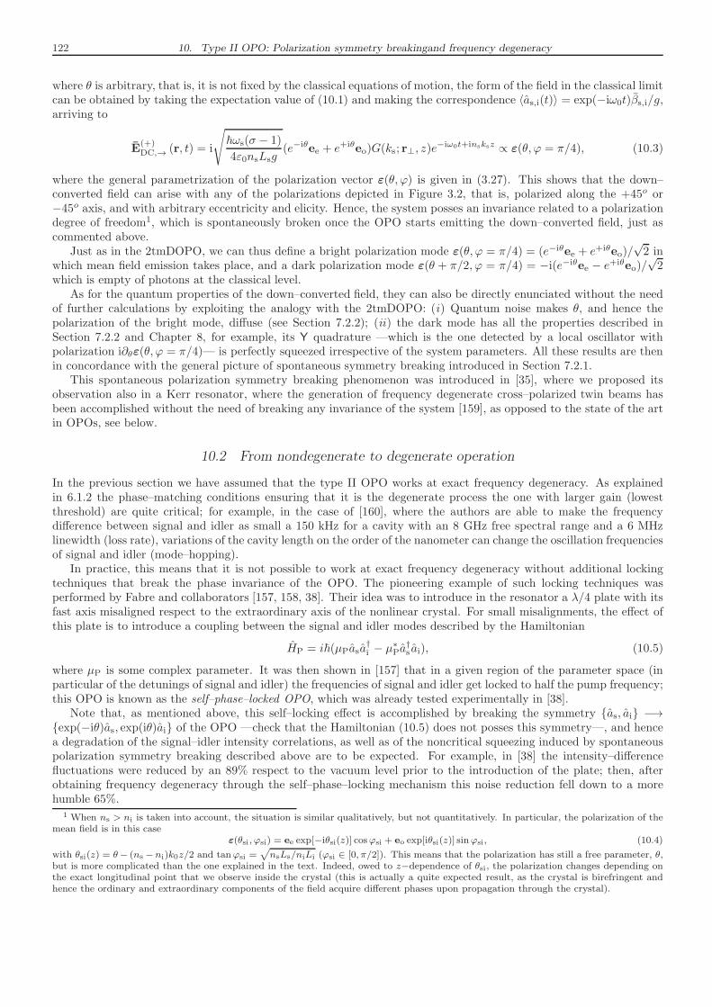
122 10. Type II OPO: Polarization symmetry breakingand frequency degeneracy

where θ is arbitrary, that is, it is not fixed by the classical equations of motion, the form of the field in the classical limitcan be obtained by taking the expectation value of (10.1) and making the correspondence 〈as,i(t)〉 = exp(−iω0t)βs,i/g,arriving to

E(+)DC,→ (r, t) = i

√

~ωs(σ − 1)

4ε0nsLsg(e−iθee + e+iθeo)G(ks; r⊥, z)e

−iω0t+insksz ∝ ε(θ, ϕ = π/4), (10.3)

where the general parametrization of the polarization vector ε(θ, ϕ) is given in (3.27). This shows that the down–converted field can arise with any of the polarizations depicted in Figure 3.2, that is, polarized along the +45o or−45o axis, and with arbitrary eccentricity and elicity. Hence, the system posses an invariance related to a polarizationdegree of freedom1, which is spontaneously broken once the OPO starts emitting the down–converted field, just ascommented above.

Just as in the 2tmDOPO, we can thus define a bright polarization mode ε(θ, ϕ = π/4) = (e−iθee + e+iθeo)/√2 in

which mean field emission takes place, and a dark polarization mode ε(θ + π/2, ϕ = π/4) = −i(e−iθee − e+iθeo)/√2

which is empty of photons at the classical level.As for the quantum properties of the down–converted field, they can also be directly enunciated without the need

of further calculations by exploiting the analogy with the 2tmDOPO: (i) Quantum noise makes θ, and hence thepolarization of the bright mode, diffuse (see Section 7.2.2); (ii) the dark mode has all the properties described inSection 7.2.2 and Chapter 8, for example, its Y quadrature —which is the one detected by a local oscillator withpolarization i∂θε(θ, ϕ = π/4)— is perfectly squeezed irrespective of the system parameters. All these results are thenin concordance with the general picture of spontaneous symmetry breaking introduced in Section 7.2.1.

This spontaneous polarization symmetry breaking phenomenon was introduced in [35], where we proposed itsobservation also in a Kerr resonator, where the generation of frequency degenerate cross–polarized twin beams hasbeen accomplished without the need of breaking any invariance of the system [159], as opposed to the state of the artin OPOs, see below.

10.2 From nondegenerate to degenerate operation

In the previous section we have assumed that the type II OPO works at exact frequency degeneracy. As explainedin 6.1.2 the phase–matching conditions ensuring that it is the degenerate process the one with larger gain (lowestthreshold) are quite critical; for example, in the case of [160], where the authors are able to make the frequencydifference between signal and idler as small a 150 kHz for a cavity with an 8 GHz free spectral range and a 6 MHzlinewidth (loss rate), variations of the cavity length on the order of the nanometer can change the oscillation frequenciesof signal and idler (mode–hopping).

In practice, this means that it is not possible to work at exact frequency degeneracy without additional lockingtechniques that break the phase invariance of the OPO. The pioneering example of such locking techniques wasperformed by Fabre and collaborators [157, 158, 38]. Their idea was to introduce in the resonator a λ/4 plate with itsfast axis misaligned respect to the extraordinary axis of the nonlinear crystal. For small misalignments, the effect ofthis plate is to introduce a coupling between the signal and idler modes described by the Hamiltonian

HP = i~(µPasa†i − µ∗Pa†s ai), (10.5)

where µP is some complex parameter. It was then shown in [157] that in a given region of the parameter space (inparticular of the detunings of signal and idler) the frequencies of signal and idler get locked to half the pump frequency;this OPO is known as the self–phase–locked OPO, which was already tested experimentally in [38].

Note that, as mentioned above, this self–locking effect is accomplished by breaking the symmetry as, ai −→exp(−iθ)as, exp(iθ)ai of the OPO —check that the Hamiltonian (10.5) does not posses this symmetry—, and hencea degradation of the signal–idler intensity correlations, as well as of the noncritical squeezing induced by spontaneouspolarization symmetry breaking described above are to be expected. For example, in [38] the intensity–differencefluctuations were reduced by an 89% respect to the vacuum level prior to the introduction of the plate; then, afterobtaining frequency degeneracy through the self–phase–locking mechanism this noise reduction fell down to a morehumble 65%.

1 When ns > ni is taken into account, the situation is similar qualitatively, but not quantitatively. In particular, the polarization of themean field is in this case

ε(θsi, ϕsi) = ee exp[−iθsi(z)] cosϕsi + eo exp[iθsi(z)] sinϕsi, (10.4)

with θsi(z) = θ− (ns −ni)k0z/2 and tanϕsi =√nsLs/niLi (ϕsi ∈ [0, π/2]). This means that the polarization has still a free parameter, θ,

but is more complicated than the one explained in the text. Indeed, owed to z−dependence of θsi, the polarization changes depending onthe exact longitudinal point that we observe inside the crystal (this is actually a quite expected result, as the crystal is birefringent andhence the ordinary and extraordinary components of the field acquire different phases upon propagation through the crystal).

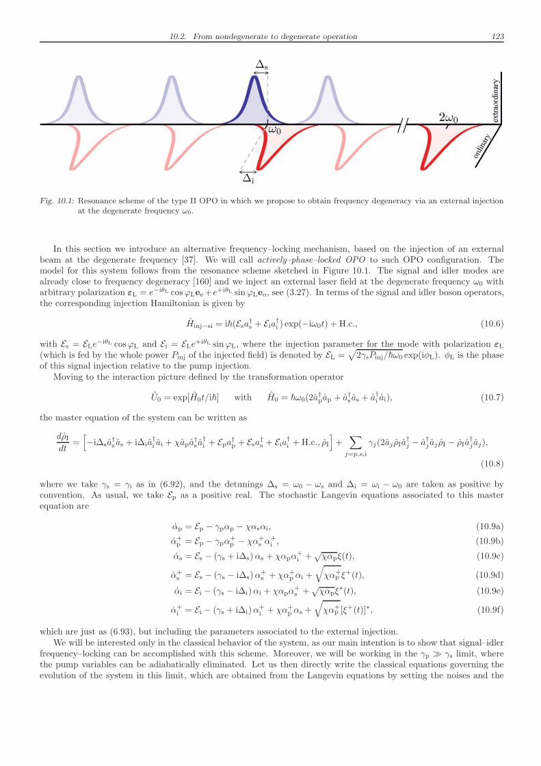
10.2. From nondegenerate to degenerate operation 123

Fig. 10.1: Resonance scheme of the type II OPO in which we propose to obtain frequency degeneracy via an external injectionat the degenerate frequency ω0.

In this section we introduce an alternative frequency–locking mechanism, based on the injection of an externalbeam at the degenerate frequency [37]. We will call actively–phase–locked OPO to such OPO configuration. Themodel for this system follows from the resonance scheme sketched in Figure 10.1. The signal and idler modes arealready close to frequency degeneracy [160] and we inject an external laser field at the degenerate frequency ω0 witharbitrary polarization εL = e−iθL cosϕLee+e

+iθL sinϕLeo, see (3.27). In terms of the signal and idler boson operators,the corresponding injection Hamiltonian is given by

Hinj−si = i~(Esa†s + Eia†i ) exp(−iω0t) + H.c., (10.6)

with Es = ELe−iθL cosϕL and Ei = ELe+iθL sinϕL, where the injection parameter for the mode with polarization εL(which is fed by the whole power Pinj of the injected field) is denoted by EL =

√

2γsPinj/~ω0 exp(iφL). φL is the phaseof this signal injection relative to the pump injection.

Moving to the interaction picture defined by the transformation operator

U0 = exp[H0t/i~] with H0 = ~ω0(2a†pap + a†s as + a†i ai), (10.7)

the master equation of the system can be written as

dρIdt

=[

−i∆sa†s as + i∆ia

†i ai + χapa

†s a†i + Epa†p + Esa†s + Eia

†i +H.c., ρI

]

+∑

j=p,s,i

γj(2aj ρIa†j − a

†j aj ρI − ρIa

†j aj),

(10.8)

where we take γs = γi as in (6.92), and the detunings ∆s = ω0 − ωs and ∆i = ωi − ω0 are taken as positive byconvention. As usual, we take Ep as a positive real. The stochastic Langevin equations associated to this masterequation are

αp = Ep − γpαp − χαsαi, (10.9a)

α+p = Ep − γpα+

p − χα+s α

+i , (10.9b)

αs = Es − (γs + i∆s)αs + χαpα+i +√χαpξ(t), (10.9c)

α+s = Es − (γs − i∆s)α

+s + χα+

p αi +

√

χα+p ξ

+(t), (10.9d)

αi = Ei − (γs − i∆i)αi + χαpα+s +√χαpξ

∗(t), (10.9e)

α+i = Ei − (γs + i∆i)α

+i + χα+

p αs +

√

χα+p [ξ

+(t)]∗, (10.9f)

which are just as (6.93), but including the parameters associated to the external injection.We will be interested only in the classical behavior of the system, as our main intention is to show that signal–idler

frequency–locking can be accomplished with this scheme. Moreover, we will be working in the γp ≫ γs limit, wherethe pump variables can be adiabatically eliminated. Let us then directly write the classical equations governing theevolution of the system in this limit, which are obtained from the Langevin equations by setting the noises and the

124 10. Type II OPO: Polarization symmetry breakingand frequency degeneracy

pump time derivatives to zero, and making the identifications α+j → α∗j . As usual, we also redefine time as τ = γst

and the coherent amplitudes as

βs = gαs exp(iθL) and βi = gαi exp(−iθL), (10.10)

so that the final equations read

βs = εseiφL −

(

1 + i∆s

)

βs + (σ − βsβi)β∗i , (10.11a)

βi = εieiφL −

(

1− i∆i

)

βi + (σ − βsβi)β∗s , (10.11b)

where we have defined the parameters

εs =g

γs|EL| cosϕL, εi =

g

γs|EL| sinϕL, and ∆j = ∆j/γs, (10.12)

while the parameters g and σ are defined as usual, see (6.53). Note that this equations are invariant under changes ofθL, and hence, the dynamics of the system are only sensitive to the parameter ϕL of the injection’s polarization.

In order to get some analytic insight, we are going to simplify the problem to what we will call symmetric configura-tion of the actively–phase–locked OPO: We assume the detunings to be equal, ∆s = ∆i = ∆, and inject with ϕL = π/4(arbitrary polarization ellipse along the ±45o axis), so that signal and idler get equally pumped, εs = εi ≡

√I. We

also choose to inject in phase with the pump injection, that is, φL = 0. With these simplifications equations (10.11)are reduced to

βs =√I −

(

1 + i∆)

βs + (σ − βsβi)β∗i , (10.13a)

βi =√I −

(

1− i∆)

βi + (σ − βsβi)β∗s . (10.13b)

These equations have the symmetry βs → β∗i , βi → β∗s , what allows us look for symmetric stationary solutions ofthe type

βs = β∗i =√I exp(iϕ). (10.14)

Note that whenever this solution exists (and is stable), the classical down–converted field emitted by the OPO will be

E(+)DC,→ (r) = i

√

~ωsI

4ε0nsLsg2(e−i(θL−ϕ)ee + ei(θL−ϕ)eo)G(ks; r⊥, z)e

−iω0t+insksz, (10.15)

where we have used (10.1) and made the correspondence 〈as,i(t)〉 = exp(−iω0t)βs,i/g. As expected, this correspondsto a field oscillating at the degenerate frequency ω0. Moreover, the polarization of this field (which is always withinthe ±45o axis) can always be chosen as linear by selecting a proper θL tuned to ϕ. In the remaining of this section westudy the conditions under which this solution exists and is stable.

It is completely trivial to show from (10.13) that the intensity I of the symmetric solution satisfies the third orderpolynomial

I = [(I + 1− σ)2 + ∆2]I, (10.16)

while its phase ϕ is uniquely determined from I as

ϕ = argI + 1− σ − i∆. (10.17)

Now, so much as happened in the previous chapter (see Figure 9.1), the polynomial (10.16) sometimes has a singlepositive definite solution, while sometimes its three roots are positive definite. By solving the equation ∂I/∂I = 0, itis simple to show that the turning points I± have the expression

I± =2

3(σ − 1)± 1

3

√

(σ − 1)2 − 3∆2 (10.18)

and hence, they exist only for σ > 1 +√3∆. For σ ≤ 1 +

√3∆ the solution is therefore single–valued.

In order to analyze the stability of this symmetric solution, we will change to a new polarization basis

εb =1√2(e−i(θL−ϕ)ee + ei(θL−ϕ)eo) and εd =

1√2i(e−i(θL−ϕ)ee − ei(θL−ϕ)eo), (10.19)

10.2. From nondegenerate to degenerate operation 125

where εb corresponds to the polarization mode excited by the symmetric solution (10.14) and εd to its orthogonal,that is, to the bright and dark modes of the system. The corresponding coherent amplitudes are written as

βb =1√2(e−iϕβs + eiϕβi) and βd =

i√2(e−iϕβs − eiϕβi), (10.20)

and satisfy the evolution equations

βb =√2I cosϕ− βb + ∆βd + (σ − β2

b/2− β2d/2)β

∗b, (10.21a)

βd = −√2I sinϕ− βd − ∆βb + (σ − β2

b/2− β2d/2)β

∗d. (10.21b)

In this new basis the symmetric solution reads

βb =√2I, βd = 0, (10.22)

and its associated stability matrix is

L =

−1− 2I σ − I ∆ 0

σ − I −1− 2I 0 ∆

−∆ 0 −1 σ − I0 −∆ σ − I −1

. (10.23)

The characteristic polynomial of this stability matrix can be factorized into two second order polynomials, namelyPI(λ) = (λ+ 1 + σ)2 + ∆2 − I2 and PII(λ) = (λ+ 1− σ + 2I)2 + ∆2 − I2. The bifurcation diagrams for the differentparameter regions are shown in Figure 10.2; now we discuss them in depth.

Let us start by studying the instabilities predicted by the first polynomial, whose roots are given by

λI± = −(1 + σ)±√

I2 − ∆2. (10.24)

Therefore, the condition ReλI± = 0 can only be satisfied for

I =

√

(1 + σ)2 + ∆2 ≡ IPB. (10.25)

The fact that the instability appears without imaginary part in the λI±, and it is located in the upper branch of theS–shaped curve (IPB > I+ for any value of the parameters), signals that it corresponds to a Pitchfork bifurcation wherea non-symmetric stationary solution βs =

√Is exp(iϕs), βi =

√Ii exp(iϕi) with Is 6= Ii borns (as we have checked

numerically, see the grey lines in Figure 10.2. This bifurcation is equivalent to the one introduced in the previouschapter when studying the effects of a signal injection in the 2tmDOPO, and can be understood as a switching on ofthe dark mode.

As for the second polynomial, its roots are given by

λII± = σ − 1− 2I ±√

I2 − ∆2. (10.26)

Note that λII± = 0 for I = I±, that is, the turning points of the S–shaped curve signal an instability. It is then simpleto check (for example numerically) that the whole middle branch connecting this instability points is unstable, asintuition says (see Figures 10.2c,d).

But λII± has yet one more instability when

I =σ − 1

2≡ IHB. (10.27)

At this instability the eigenvalues become purely imaginary, in particular, λII± = ±iωHB with ωHB =√

∆2 − (σ − 1)2/4,

and hence it corresponds to a Hopf bifurcation. Note that IHB is negative for σ < 1, while ωHB becomes imaginaryfor σ > 1 + 2∆, and hence the Hopf bifurcation only exists in the region 1 < σ < 1 + 2∆. It is simple to check thatIHB is always below IPB and I−; in particular, it borns at I = 0 for σ = 1, and climbs the I − I curve as σ increasesuntil it dies at I = I− for σ = 1+ 2∆ (see Figures 10.2b,c,d). The portion of the curve with I < IHB is unstable, andno stationary solutions can be found there, as the stable states correspond in this case to periodic orbits (as we havechecked numerically, see Figures 10.2b,c,d). This is also quite intuitive because when no injection is present, that is,for I = 0, we know that the stable states of the OPO above threshold are the ones with the signal and idler beamsoscillating at the non-degenerate frequencies ωs = ω0 +∆ and ωi = ω0 −∆, which in the picture we are working onmeans βs(τ) ∝ exp(−i∆τ), βi(τ) ∝ exp(i∆τ).

This analysis proves that there exist regions in the parameter space where the frequencies of the signal and idlerbeams are locked to the degenerate one, and hence active–locking can be a good alternative to the self–locking techniquealready proposed for type II OPOs [157, 158, 38].

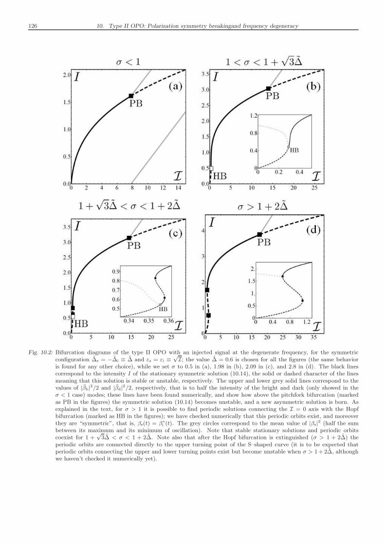
126 10. Type II OPO: Polarization symmetry breakingand frequency degeneracy

Fig. 10.2: Bifurcation diagrams of the type II OPO with an injected signal at the degenerate frequency, for the symmetricconfiguration ∆s = −∆i ≡ ∆ and εs = εi ≡

√I; the value ∆ = 0.6 is chosen for all the figures (the same behavior

is found for any other choice), while we set σ to 0.5 in (a), 1.98 in (b), 2.09 in (c), and 2.8 in (d). The black linescorrespond to the intensity I of the stationary symmetric solution (10.14), the solid or dashed character of the linesmeaning that this solution is stable or unstable, respectively. The upper and lower grey solid lines correspond to thevalues of |βb|2/2 and |βd|2/2, respectively, that is to half the intensity of the bright and dark (only showed in theσ < 1 case) modes; these lines have been found numerically, and show how above the pitchfork bifurcation (markedas PB in the figures) the symmetric solution (10.14) becomes unstable, and a new asymmetric solution is born. Asexplained in the text, for σ > 1 it is possible to find periodic solutions connecting the I = 0 axis with the Hopfbifurcation (marked as HB in the figures); we have checked numerically that this periodic orbits exist, and moreoverthey are “symmetric”, that is, βs(t) = β∗

i (t). The grey circles correspond to the mean value of |βs|2 (half the sumbetween its maximum and its minimum of oscillation). Note that stable stationary solutions and periodic orbitscoexist for 1 +

√3∆ < σ < 1 + 2∆. Note also that after the Hopf bifurcation is extinguished (σ > 1 + 2∆) the

periodic orbits are connected directly to the upper turning point of the S–shaped curve (it is to be expected thatperiodic orbits connecting the upper and lower turning points exist but become unstable when σ > 1+ 2∆, althoughwe haven’t checked it numerically yet).

11. DOPOS TUNED TO ARBITRARY TRANSVERSE FAMILIES

So far we have studied DOPOs tuned to a fundamental TEM00 mode (Section 6.3) and to the first family of transversemodes at the signal frequency (Section 7.2.2 and Chapters 8 and 9). The former was introduced as an example of asystem showing bifurcation squeezing, while we proposed the later as a playground where studying the phenomenonof noncritical squeezing induced by spontaneous symmetry breaking. It is then natural to generalize the study to aDOPO tuned to an arbitrary family of transverse modes at the signal frequency, and this is what this final chapter isintended to do. We remind that a given family, say family f , posses f + 1 transverse modes having orbital angularmomenta ±f,±(f−2), ...,±l0, with l0 equal to 0 for even families and 1 for the odd ones, so that the part signal fieldpropagating along +ez can be written in the Laguerre–Gauss basis as (from now on all the sums over l are assumedto run over the set l ∈ f, f − 2, ..., l0)

E(+)s,→ (r) = i

√

~ωs

4ε0nsLsee∑

±l

alL(f−|l|)/2,l (ks; r⊥, z) einsksz; (11.1)

hence, for f ≥ 2 this DOPO has more than one parametric down–conversion channel available, that is, a pump photoncan decay into any pair of opposite angular momentum signal photons. Armed with the things that we have learnedso far (bifurcation squeezing, pump clamping, and spontaneous symmetry breaking), the properties of such systemwill be quite intuitive; in fact, this is the system in which we originally predicted the phenomenon of OPO clamping[29] that was introduced in a general way in Section 7.1.

What is interesting about this particular implementation of a multi–mode DOPO that we may call f–transverse–family DOPO is that, as we will show in Section 11.4, by tuning the thickness of the pump mode (what can be doneby using monolithic designs in which the cavities for the pump and signal modes are independent, or singly–resonantOPOs) one can find many transverse modes with large levels of squeezing, hence creating a highly nonclassical andmulti–mode beam.

11.1 The model

As in the previous cases, the general model for intracavity down–conversion that we developed in Section 6.2 coversalso the configuration that we are dealing with in this chapter. In particular, the down–conversion Hamiltonian can beobtained by particularizing (6.42) to the current scenario in which the set of transverse modes resonating at the signalfrequency is the corresponding to the Laguerre–Gauss modes L(f−l)/2,±l (k; r⊥, z)l∈f,f−2,...,l0. Denoting by ap andal the annihilation operators for pump photons and signal photons with orbital angular momentum l, respectively, weget

Hc = i~∑

l

χl1 + δ0,l

apa†l a†−l +H.c., (11.2)

where

χl = 3lcχ(2)oee(2ω0;ω0, ω0)

√

~ω30

2ε0n3cL

3opt

∫ +∞

0

rdrG(kp; r)[

Rl(f−l)/2(ks; r)]2

. (11.3)

Note that the larger is the OAM of the down–converted pair, the smaller is the overlapping between the squareof Rl(f−l)/2(ks; r) and the Gaussian pump profile G(kp; r), what comes from the fact that the modes are thicker thelarger their angular OAM is, and hence the following ordering of the couplings holds

χf < χf−2 < · · · < χl0 , (11.4)

that is, the lowest OAM modes are the ones coupled more strongly to the pump.

128 11. DOPOs tuned to arbitrary transverse families

The master equation associated to the f–transverse–family DOPO in a picture rotated to the laser frequency andin which everything is assumed to be resonant reads then

dρIdt

=

[

∑

l

χl1 + δ0,l

apa†l a†−l + Epa†p +H.c., ρI

]

+∑

j=p,±l

γj(2aj ρIa†j − a

†j aj ρI − ρIa

†j aj); (11.5)

now, assuming that all the signal modes have the same loss rate γs, we can map this master equation into the followingLangevin equations within the positive P representation:

αp = Ep − γpαp −∑

l

χl1 + δ0,l

αlα−l, (11.6a)

α+p = Ep − γpα+

p −∑

l

χl1 + δ0,l

α+l α

+−l, (11.6b)

αl = −γsαl + χlαpα+−l +

√χlαpξl(t), (11.6c)

α+l = −γsα+

l + χlα+p α−l +

√

χlα+p ξ

+l (t), (11.6d)

α−l = −γsα−l + χlαpα+l +√χlαpξ

∗l (t), (11.6e)

α+−l = −γsα+

−l + χlα+p αl +

√

χlα+p

[

ξ+l (t)]∗, (11.6f)

where all the various complex noises satisfy the usual statistical properties (6.94) and are independent.As usual, we now rewrite the equations in terms of the following normalized variables

τ = γst, βj(τ) =χl0

γs√

γp/γjαj(t), ζj(τ) =

1√γsξj(t), (11.7)

arriving to

βp = κ

[

σ − βp −∑

l

rl1 + δ0,l

βlβ−l

]

, (11.8a)

β+p = κ

[

σ − β+p −

∑

l

rl1 + δ0,l

β+l β

+−l

]

, (11.8b)

βl = −βl + rlβpβ+−l + g

√

rlβpζl(τ), (11.8c)

β+l = −β+

l + rlβ+p β−l + g

√

rlβ+p ζ

+l (τ), (11.8d)

β−l = −β−l + rlβpβ+l +√rlαpζ

∗l (τ), (11.8e)

β+−l = −β+

−l + rlβ+p βl +

√

rlβ+p

[

ζ+l (τ)]∗, (11.8f)

where in this case the parameters are defined as

κ = γp/γs, σ = χl0Ep/γpγs, g = χl0/√γpγs, rl = χl/χl0 . (11.9)

Note that 0 < rl ≤ 1, where the equality holds only for l = l0.It will be convenient for future purposes to remind that instead of the Laguerre–Gauss basis, one could describe

the system through the Hybrid Laguerre–Gauss modes Yj,(f−l)/2,l (ks; r⊥, z)j=c,sl∈f,f−2,...,l0, see (3.49). For l = 0 the

HLG and LG modes coincide and are rotationally symmetric, while for l 6= 0 the HLG modes have a well definedorientation in the transverse plane (see Figure 3.5). The annihilation operators for HLG photons are related to theLG ones by

ac,l = (a+l + a−l)/√2, as,l = i(a+l − a−l)/

√2. (11.10)

11.2 Classical emission

Based on the phenomenon of pump clamping that we introduced in Section 7.1, it is completely trivial to understandthe classical behavior of the f–transverse–family DOPO; let’s see this.

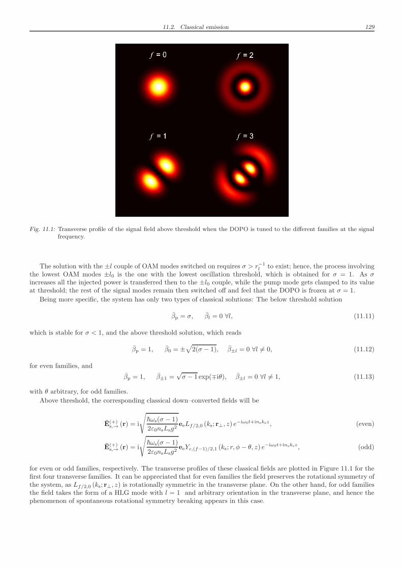
11.2. Classical emission 129

Fig. 11.1: Transverse profile of the signal field above threshold when the DOPO is tuned to the different families at the signalfrequency.

The solution with the ±l couple of OAM modes switched on requires σ > r−1l to exist; hence, the process involvingthe lowest OAM modes ±l0 is the one with the lowest oscillation threshold, which is obtained for σ = 1. As σincreases all the injected power is transferred then to the ±l0 couple, while the pump mode gets clamped to its valueat threshold; the rest of the signal modes remain then switched off and feel that the DOPO is frozen at σ = 1.

Being more specific, the system has only two types of classical solutions: The below threshold solution

βp = σ, βl = 0 ∀l, (11.11)

which is stable for σ < 1, and the above threshold solution, which reads

βp = 1, β0 = ±√

2(σ − 1), β±l = 0 ∀l 6= 0, (11.12)

for even families, and

βp = 1, β±1 =√σ − 1 exp(∓iθ), β±l = 0 ∀l 6= 1, (11.13)

with θ arbitrary, for odd families.

Above threshold, the corresponding classical down–converted fields will be

E(+)s,→ (r) = i

√

~ωs(σ − 1)

2ε0nsLsg2eeLf/2,0 (ks; r⊥, z) e

−iω0t+insksz , (even)

E(+)s,→ (r) = i

√

~ωs(σ − 1)

2ε0nsLsg2eeYc,(f−1)/2,1 (ks; r, φ− θ, z) e−iω0t+insksz, (odd)

for even or odd families, respectively. The transverse profiles of these classical fields are plotted in Figure 11.1 for thefirst four transverse families. It can be appreciated that for even families the field preserves the rotational symmetry ofthe system, as Lf/2,0 (ks; r⊥, z) is rotationally symmetric in the transverse plane. On the other hand, for odd familiesthe field takes the form of a HLG mode with l = 1 and arbitrary orientation in the transverse plane, and hence thephenomenon of spontaneous rotational symmetry breaking appears in this case.

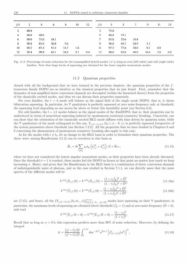
130 11. DOPOs tuned to arbitrary transverse families

Fig. 11.2: Percentage of noise reduction for the nonamplified hybrid modes l 6= l0 lying in even (left table) and odd (right table)families. Note that large levels of squeezing are obtained for the lower angular momentum modes.

11.3 Quantum properties

Armed with all the background that we have learned in the previous chapters, the quantum properties of the f–transverse–family DOPO are as intuitive as the classical properties that we just found. First, remember that thedynamics of non-amplified down–conversion channels are decoupled (within the linearized theory) from the propertiesof the classically excited modes, and then we can discuss their properties separately.

For even families, the l = 0 mode will behave as the signal field of the single–mode DOPO, that is, it showsbifurcation squeezing. In particular, its Y quadrature is perfectly squeezed at zero noise frequency only at threshold,the squeezing level degrading as one moves far above or below this instability point (see Section 6.3).

For odd families, the l = ±1 modes behave as the signal modes of the 2tmDOPO, that is, their properties can beunderstood in terms of noncritical squeezing induced by spontaneous rotational symmetry breaking. Concretely, onecan show that the orientation of the classically excited HLG mode diffuses with time driven by quantum noise, whilethe Y quadrature of the mode orthogonal to this one, Ys,(f−1)/2,1 (ks; r, φ− θ, z), is perfectly squeezed irrespective ofthe system parameters above threshold (see Section 7.2.2). All the properties that we have studied in Chapters 8 and9 concerning the phenomenon of spontaneous symmetry breaking also apply to this case.

As for the modes with l 6= l0, let us change to the HLG basis in order to formulate their quantum properties. Thethree–wave–mixing Hamiltonian (11.2) can be rewritten in this basis as

Hc = i~∑

l 6=l0

χlap

(

a†2c,l + a†2s,l

)

/2 + H.c., (11.15)

where we have not considered the lowest angular momentum modes, as their properties have been already discussed.Once the threshold σ = 1 is reached, these modes feel the DOPO as frozen at that point no matter how much we keepincreasing σ. Hence, and given that the Hamiltonian in the HLG basis is a combination of down–conversion channelsof indistinguishable pairs of photons, just as the case studied in Section 7.1.1, we can directly asses that the noisespectra of the different modes will be

V out(Xc,l; Ω) = V out(Xs,l; Ω) =(1 + rlβp)

2 + Ω2

(1 − rlβp)2 + Ω2, (11.16a)

V out(Yc,l; Ω) = V out(Ys,l; Ω) =(1− rlβp)2 + Ω2

(1 + rlβp)2 + Ω2, (11.16b)

see (7.15), and hence, all the Yj,(f−l)/2,l (ks; r⊥, z)j=c,sl∈f,f−2,...,l0+2 modes have squeezing on their Y quadrature; in

particular, the maximum levels of squeezing are obtained above threshold (βp = 1) and at zero noise frequency (Ω = 0),and read

V out(Yc,l; Ω = 0) = V out(Ys,l; Ω = 0) =(1 − rl)2(1 + rl)2

. (11.17)

Recall that as long as rl > 0.5, this expression predicts more than 90% of noise reduction. Moreover, by defining theintegral

Il =[(f − l)/2]![(f + l)/2]!

∫ +∞

0

due−2u2

u2l+1[

Ll(f−l)/2(u2)]2

, (11.18)

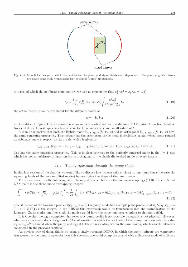
11.4. Tuning squeezing through the pump shape 131

Fig. 11.3: Monolithic design in which the cavities for the pump and signal fields are independent. The pump (signal) mirrorsare made completely transparent for the signal (pump) frequencies.

in terms of which the nonlinear couplings are written as (remember that w2p/w

2s = λp/λs = 1/2)

χl =3

2

lcwsχ(2)oee(2ω0;ω0, ω0)

√

8~ω30

π3ε0n3cL

3opt

Il, (11.19)

the actual ratios rl can be evaluated for the different modes as

rl = Il/Il0 ; (11.20)

in the tables of Figure 11.2 we show the noise reduction obtained for the different OAM pairs of the first families.Notice that the largest squeezing levels occur for large values of f and small values of l.

It is to be remarked that both the Hybrid mode Yc,(f−l)/2,l (ks; r⊥, z) and its orthogonal Ys,(f−l)/2,l (ks; r⊥, z) havethe same squeezing properties. This means that the orientation of the mode is irrelevant, as an hybrid mode rotatedan arbitrary angle ψ respect to the x axis, which is given by

Yc,(f−l)/2,l (ks; r, φ− ψ, z) = Yc,(f−l)/2,l (ks; r⊥, z) cos lψ + Ys,(f−l)/2,l (ks; r⊥, z) sin lψ, (11.21)

also has the same squeezing properties. This is in clear contrast to the perfectly squeezed mode in the l = 1 casewhich has not an arbitrary orientation but is orthogonal to the classically excited mode at every instant.

11.4 Tuning squeezing through the pump shape

In this last section of the chapter we would like to discuss how we can take rl closer to one (and hence increase thesqueezing levels of the non-amplified modes) by modifying the shape of the pump mode.

The idea comes from the following fact. The only difference between the nonlinear couplings (11.3) of the differentOAM pairs is the three–mode overlapping integral

∫ +∞

0

rdrG(kp; r)[

Rl(f−l)/2(ks; r)]2

=1

2π

∫

R2

d2r⊥G(kp; r⊥, z = 0)L(f−l)/2,l(ks; r⊥, z = 0)L∗(f−l)/2,l(ks; r⊥, z = 0);

(11.22)

now, if instead of the Gaussian profile G(kp; r⊥, z = 0) the pump mode had a simple plane profile, that is, G(kp; r⊥, z =0) → C 6= C(r⊥), the integral in the RHS of this expression would be transformed into the normalization of theLaguerre–Gauss modes, and hence all the modes would have the same nonlinear coupling to the pump field.

It is true that having a completely homogeneous pump profile is not possible because it is not physical. However,what we can actually do is design an OPO configuration in which the spot size of the pump mode exceeds the valuewp = ws/

√2 obtained when the pump and signal fields are resonating within the same cavity, which was the situation

considered in the previous sections.An obvious way of doing this is by using a singly–resonant DOPO, in which the cavity mirrors are completely

transparent at the pump frequencies; was this the case, one could pump the crystal with a Gaussian mode of arbitrary

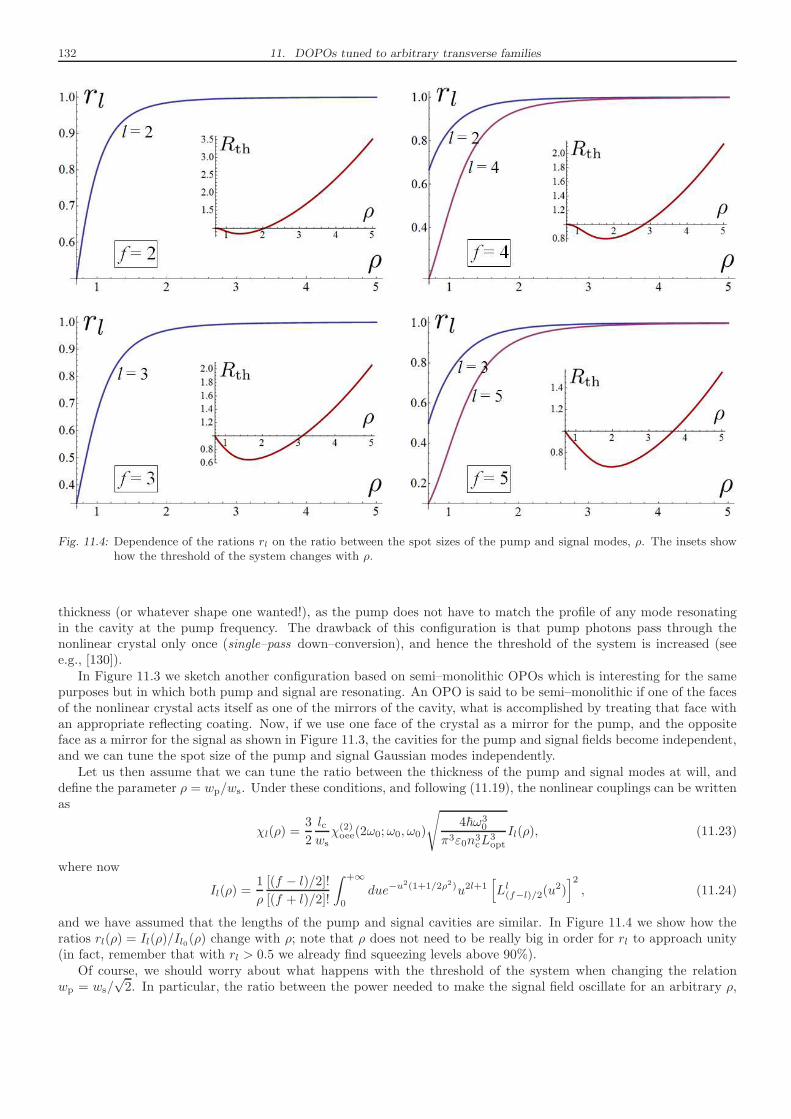
132 11. DOPOs tuned to arbitrary transverse families

Fig. 11.4: Dependence of the rations rl on the ratio between the spot sizes of the pump and signal modes, ρ. The insets showhow the threshold of the system changes with ρ.

thickness (or whatever shape one wanted!), as the pump does not have to match the profile of any mode resonatingin the cavity at the pump frequency. The drawback of this configuration is that pump photons pass through thenonlinear crystal only once (single–pass down–conversion), and hence the threshold of the system is increased (seee.g., [130]).

In Figure 11.3 we sketch another configuration based on semi–monolithic OPOs which is interesting for the samepurposes but in which both pump and signal are resonating. An OPO is said to be semi–monolithic if one of the facesof the nonlinear crystal acts itself as one of the mirrors of the cavity, what is accomplished by treating that face withan appropriate reflecting coating. Now, if we use one face of the crystal as a mirror for the pump, and the oppositeface as a mirror for the signal as shown in Figure 11.3, the cavities for the pump and signal fields become independent,and we can tune the spot size of the pump and signal Gaussian modes independently.

Let us then assume that we can tune the ratio between the thickness of the pump and signal modes at will, anddefine the parameter ρ = wp/ws. Under these conditions, and following (11.19), the nonlinear couplings can be writtenas

χl(ρ) =3

2

lcwsχ(2)oee(2ω0;ω0, ω0)

√

4~ω30

π3ε0n3cL

3opt

Il(ρ), (11.23)

where now

Il(ρ) =1

ρ

[(f − l)/2]![(f + l)/2]!

∫ +∞

0

due−u2(1+1/2ρ2)u2l+1

[

Ll(f−l)/2(u2)]2

, (11.24)

and we have assumed that the lengths of the pump and signal cavities are similar. In Figure 11.4 we show how theratios rl(ρ) = Il(ρ)/Il0(ρ) change with ρ; note that ρ does not need to be really big in order for rl to approach unity(in fact, remember that with rl > 0.5 we already find squeezing levels above 90%).

Of course, we should worry about what happens with the threshold of the system when changing the relationwp = ws/

√2. In particular, the ratio between the power needed to make the signal field oscillate for an arbitrary ρ,

11.4. Tuning squeezing through the pump shape 133

and that for ρ = 1/√2 is given by

Rth(ρ) =Pth(ρ)

Pth(ρ = 1/√2)

=χ2l0(ρ = 1/

√2)

χ2l0(ρ)

=I2l0(ρ = 1/

√2)

I2l0(ρ), (11.25)

as follows from (4.40), (11.9), and (11.23). This expression is plotted in the insets of Figure 11.4 for the differentfamilies. These figures show that the changes in the threshold are quite reasonable, and moreover, the threshold iseven lowered respect to the ρ = 1/

√2 case for small enough ratios ρ.

134 11. DOPOs tuned to arbitrary transverse families

12. CONCLUSIONS AND OUTLOOK

12.1 Summary of the original research on OPOs

This thesis has been devoted to the study of some new properties of optical parametric oscillators (OPOs). Suchdevices consist of an optical cavity embedding a second order nonlinear crystal, which, when pumped with an externallaser beam at frequency ωp = 2ω0, is able to generate light at frequencies ωs and ωi such that ωp = ωs + ωi, throughthe process of parametric down–conversion (the ωp, ωs, and ωi fields are called, respectively, pump, signal, and idler).The down–conversion process is known as degenerate when the signal and idler modes have the same frequency ω0,and type I when they have the same polarization (if they are generated in orthogonal, linearly polarized modes, wetalk then about type II down–conversion).As stressed in the Introduction, the first two–thirds of the dissertation have consisted on a self–contained discussionabout the basic physics behind these devices. Here we would like to remark the following well known properties ofOPOs (see Section 1.2.1 for an extensive summary of this introductory part):

• From a classical point of view, the interplay between parametric down–conversion and cavity losses forces thepump power (denoted along the thesis by the dimensionless parameter σ) to go above some threshold level(σ = 1) in order to make the signal–idler fields oscillate. Hence, at σ = 1 the system shows a bifurcation inwhich the OPO passes from a steady state with the down–converted fields switched off, to a new steady state inwhich these are switched on (much like in the laser).

• Working with type I, degenerate down–conversion, we simply talk about a degenerate OPO (DOPO). If inaddition the signal and idler modes are generated with in the same transverse mode (typically a TEM00 mode),we talk about a single–mode DOPO. It is possible to show that in such system the down–converted field is ina squeezed state, that is, one of its quadratures has fluctuations below the vacuum (shot noise) level. However,this squeezing is only large when working close to the bifurcation: We say that it is a critical phenomenon.

• When the down–converted photons are distinguishable in frequency or/and polarization, we have shown thatthe joint state of the signal and idler modes corresponds to an entangled state in which these share correlationswhich go beyond what is classically allowed. Again, the entanglement level is large only when working close tothreshold.However, in this case there is one highly squeezed observable at any pump level above threshold: The signal–idlerintensity difference. We say then that signal and idler are twin beams, as they have perfectly correlated photonnumbers.

These well known results were the starting point of the research developed in this thesis; in the remaining of thissection we make a summary of the main original results that we have found (numbering of this list follows the chaptersand sections of the dissertation):

7. In the first completely original chapter we have introduced the concept of multi–mode OPO as that havingseveral down–conversion channels available for a single pump mode. We have argued that this is actually thenatural way in which OPOs operate, either because it is impossible to forbid the existence of other transversemodes close to the one in which we would like to operate, or because the phase matching curve is wide enoughas to include more than a single signal–idler frequency pair.We have then introduced two phenomena characteristic of multi–mode OPOs, phenomena which are consideredby the PhD candidate as the most important contribution of the thesis: Pump clamping and spontaneoussymmetry breaking. As we explain now, their main interest is that they offer new means for generating squeezed(or entangled) light, with the incentive that the squeezing is noncritical, that is, independent of the systemparameters.

7.1. Let us first explain the key points describing the phenomenon of pump clamping:

136 12. Conclusions and outlook

∗ In general, the different down–conversion channels of the multi–mode OPO will have different thresh-olds, depending these on the coupling to the pump, the detuning, and the loss rates of the modesinvolved in the particular process.

∗ Classically, only the channel with the lowest threshold can be amplified, that is, the processes withhigher thresholds remain switched off no matter how much we increase σ.

∗ What is interesting is that once the lowest threshold mode is generated, the non-amplified modes feel asif the OPO was frozen at the bifurcation, even if we change the actual pump injection. This applies alsoto their quantum properties, that is, the modes of the non-amplified channels will have the squeezingor entanglement that they are supposed to have below their oscillation threshold, irrespective of thesystem parameters.

Hence, our first prediction has been that, above threshold, apart from the bright signal–idler modes whichbehave as the ones in the single–channel OPO (bifurcation squeezing or entanglement), the output of ageneral OPO has a lot more signal–idler pairs with some squeezing or entanglement, their actual levels de-pending on the distance between their thresholds and the lowest threshold of the system (the true threshold).

7.2.1. We have introduced the basic idea behind spontaneous symmetry breaking in an abstract way as follows:

∗ Suppose that we work with an OPO which is invariant under changes of some continuous degree offreedom of the down–converted field, say ǫ, which we have denoted by “free parameter” all along thedissertation. Above threshold, the down–converted field, say Eǫ(r, t) —we explicitly introduce the freeparameter in the field—, is not zero, and when the OPO starts emitting it, a particular value of thefree parameter is chosen according to the particular fluctuations from which the field is built up. Wesay that ǫ is chosen through spontaneous symmetry breaking.

∗ Let’s think now about what quantum theory might introduce to this classical scenario. First, asvariations of the FP do not affect the system (what mathematically is reflected in the appearance of aGoldstone mode in the matrix governing the linear evolution of the system, that is, a mode with nulleigenvalue), quantum noise is expected to make it fluctuate without opposition, eventually making itbecome completely undetermined.

∗ Then, invoking now the uncertainty principle, the complete indetermination of a system’s variable allowsfor the perfect determination of its corresponding momentum, meaning this that we could expect perfectsqueezing in the quadrature selected by the local oscillator −i∂ǫEǫ(r, t) in an homodyne detectionscheme.

∗ Finally, as this process relies only on the generation of the down–converted field, this perfect squeezingis expected to be independent of the distance to threshold, as long as we are above the bifurcationpoint.

The first proof of such an intuitive reasoning was offered through the study of a DOPO with plane mirrors[30, 31], where transverse patterns as well as cavity solitons have been predicted to appear above threshold[137, 138], hence breaking the translational symmetry of the system. Most of the present thesis has beendevoted to study several aspects of the phenomenon of spontaneous symmetry breaking, but we havedesigned a much more simple (and realistic) DOPO configuration for that matter.

7.2.2,8. The system we have used to study in depth the phenomenon of spontaneous symmetry breaking is a DOPO (hencesignal and idler have the same frequency and polarization) pumped by a TEM00 mode, and whose cavity is tunedso that the first family of transverse modes resonates at the down–converted frequency. Under this circumstancesthe down–converted photons are created in opposite orbital angular momentum (OAM) Laguerre–Gauss modes,and, consequently, we have called two–transverse–mode DOPO (2tmDOPO) to this system.Let us summarize now the main results that we have found in this system.

7.2.2. In connection with the general picture of 7.2.1, these are the properties of the system:

∗ A weighted superposition of two ±1 Laguerre–Gauss modes can be seen as a TEM10 mode, whose ori-entation in the transverse plane is given by half the phase–difference between the underlying Laguerre–Gauss modes. Hence, owed to the rotational invariance of the cavity, classical emission takes placein a TEM10 mode with an arbitrary orientation in the transverse plane (mathematically this is clearbecause the 2tmDOPO classical equations are invariant against changes in the relative phase betweenthe Laguerre–Gauss modes).

12.1. Summary of the original research on OPOs 137

Hence, once the threshold is crossed and the orientation is chosen according to the particular initialfluctuations, the rotational symmetry is spontaneously broken, and we can talk about a bright mode(the generated one which breaks the symmetry) and a dark mode (the mode orthogonal to the generatedone).

∗ Quantum noise is able to make the bright TEM10 mode rotate randomly in the transverse plane.Mathematically, this is reflected in the appearance of a Goldstone mode in the matrix governing thelinear evolution of the fluctuations above threshold. The null eigenvalue of this mode allows quantumnoise to change the orientation of the bright mode without opposition. Though continuously increasingwith time, this rotation of the classically excited pattern is quite slow when working above threshold.

∗ As for the squeezing properties, it has been proved that the bright mode has the same behavior asthe single–mode DOPO, i.e., large levels of squeezing appear only close to threshold. On the otherhand, accompanying the Goldstone mode it appears another mode whose associated eigenvalue takesthe minimum possible value (−2).Together, the Goldstone mode and the maximally damped mode are responsible of the remarkableproperties of the dark mode: Its Y quadrature is perfectly squeezed at any pump level above threshold,while its X quadrature carries only with vacuum fluctuations (in apparent violation of the uncertaintyprinciple).This is in full agreement with the abstract picture of the phenomenon offered in 7.2.1, as the dark modecoincides (up to a π/2 phase) with the OAM of the bright mode.

8.1. We have proved that the apparent violation of the uncertainty principle is just that, apparent, as theconjugate pair of the squeezed quadrature is not another quadrature but the orientation of the brightmode, which in fact is completely undetermined in the long time term.

8.2. Next we have pointed out that in order to measure the quantum properties of the dark mode via homodynedetection, one has to use a TEM10 local oscillator that is perfectly matched to the orientation of this modeat any time. However, the mode is rotating randomly, which seems to make impossible the perfect matching.For this reason we have studied the situation in which the local oscillator is matched to the dark mode’sorientation only at the initial time, remaining fixed during the detection time.We have shown that arbitrarily large levels of noise reduction can be obtained even in this case if the phaseof the local oscillator is exactly π/2. We then considered phase deviations up to 2 (1.5 seems to be thecurrent experimental limit [5, 6]), comparing the results with those predicted for the single–mode DOPO;similar levels are obtained for both, with the advantage that in the 2tmDOPO this level is independent ofthe distance from threshold, and hence, noncritical.

8.3. We have also shown that the assumptions made in order to analytically solve the problem are not theresponsible for the quantum properties of the dark mode. In particular, we have used numerical simulationsto show that these analytic predictions coincide with those of the complete nonlinear stochastic equationsdescribing the system.

9. In this chapter we have studied the classical and quantum dynamics of the 2tmDOPO when a TEM10 beam isinjected at the signal frequency. This study was motivated by experimental reasons: On one hand, this injectionis customarily used in real DOPOs to stabilize the cavity, so that, in particular, the signal resonance is locked tothe desired value (active locking); on the other, in the 2tmDOPO, and given that down–conversion is a stimulatedprocess, we think that the injection of a TEM10 mode could also lock the orientation of the bright mode, whatseems highly recommendable from the detection point of view.These are the main results that we have found:

9.2. Let’s start with the classical dynamics. For signal injections below some threshold, the system posses aunique, stable solution in which the TEM01 (the non-injected mode) remains switched off. However, abovethis injection threshold both the TEM10 and TEM01 modes become populated. Hence, the system possesa new bifurcation linked to the switching on of the non-injected mode.This bifurcation is present for any σ, and in particular it exists also for σ = 0, when the DOPO runs as asecond harmonic generator (as in this case the 2ω0 field is generated from the ω0 injection); of course inthis case the threshold is independent of the injection’s phase, as there is no other phase reference. Forσ > 0 this is no longer the case: The threshold is maximum (minimum) when the signal injection is inphase (anti–phase) with the pump injection.Surprisingly, working in anti–phase and when σ ≥ 1, there is no threshold for the generation of the TEM01

mode. On the other hand, in the in–phase case there exists a clear threshold below which the bright modeis locked to the injected TEM10 mode, just as we wanted to prove.

138 12. Conclusions and outlook

9.3. As for the quantum properties, we have proved that the TEM01 mode has large levels of squeezing in allthe region below their generation threshold, hence proving that the TEM10 injection does not degrade toomuch the squeezing capabilities of the 2tmDOPO.This insensitivity to the injection (in particular we have proved that it is far much insensitive to the injectionthan the single–mode DOPO, the configuration customarily used in experiments) comes from the fact thatthe TEM01 mode shows perfect squeezing at the instability point leading to its activation.

10. In this chapter we have studied type II OPOs tuned to the TEM00 mode for all the frequencies involved in thedown–conversion process. We had a twofold intention:

10.1. On one hand, we wanted to generalize the phenomenon of spontaneous symmetry breaking to the polar-ization degrees of freedom of light. In particular, we have shown that when the down–conversion processis also frequency degenerate, the system is isomorphic to the 2tmDOPO, where the role of the oppositeorbital angular momenta are now played by the orthogonal linear polarizations of the signal–idler modes.We have then proved that the behavior expected after the general reasoning of Section 7.2.1 applies: Clas-sical emission takes place in an elliptically polarized mode, and the free parameter of this system (therelative phase between signal and idler) is related now to the eccentricity of the corresponding polarizationellipse; quantum noise is responsible for a diffusion process of this polarization parameter, which eventuallybecomes completely undetermined; the Y quadrature of the dark mode, which in this case consists on themode orthogonally polarized to the bright one, has perfect squeezing at any pump level above threshold.

10.2. However, we have pointed out that in real experiments it seems not possible to obtain frequency degeneracyin OPOs. In the case of type II operation, frequency degeneracy can be obtained by introducing a birefrin-gent element inside the cavity (self–phase–locked type II OPOs), but this breaks the polarization symmetryof the system, hence destroying the phenomenon of spontaneous symmetry breaking. Nevertheless, we haveargued that a residual squeezing should be present after this explicit symmetry breaking, and that it wasactually observed (but not interpreted a residue of the symmetry breaking) some years ago [38].We then show that frequency degeneracy might as well be obtained by injecting an external laser beam atthe degenerate frequency (actively–phase-locked type II OPOs). Moreover, we have studied the completebifurcation diagram of this system in the simple case of having opposite detunings for the signal and idlermodes, showing that there are regimes in which stationary solutions coexist with periodic orbits.

11. Motivated by the fact that we already studied DOPOs tuned to the fundamental TEM00 mode at the subharmonic(single–mode DOPOs), as well as DOPOs tuned to the first family of transverse modes (2tmDOPOs), in the lastoriginal chapter of the thesis we have studied what happens when the DOPO is tuned to an arbitrary familyof transverse modes at the signal frequency. Note that family f contains Laguerre–Gauss modes with orbitalangular momenta ±f,±(f − 2), ...,±l0, with l0 equal to 0 for even families and 1 for the odd ones.The results have been actually very intuitive based on the phenomena that we studied in the previous chapters.In particular:

11.2. Given that the lowest orbital angular momenta of the family are the ones which couple the strongest to thepump (so that they have the lowest threshold), they will be the ones classically amplified above threshold,while the rest of modes will remain switched off.For even families this means that the bright mode will consist in a 0 OAM mode, and hence the rotationalsymmetry of the system will be preserved; on the other hand, the bright mode for the case of odd familieswill consist in a superposition of two ±1 OAM modes (a Hybrid Laguerre–Gauss mode), and hence therotational symmetry will be spontaneously broken.

11.3. As for the quantum properties, they are very simple to guess as well. First, and given that the dynamics ofthe non-amplified modes decouple from the ones of the amplified ones, the 0 OAM mode of the even–familycase will behave as the signal field of the single–mode DOPO (bifurcation squeezing); similarly, the ±1OAM modes of the odd–family case will behave as the ones in the 2tmDOPO (the Hybrid Laguerre–Gaussmode generated above threshold and its orthogonal will behave, respectively, as the bright and dark modesof the 2tmDOPO).On the other hand, and this is the most relevant result, the properties of the higher OAM modes aredictated by the phenomenon of pump clamping, that is, the Hybrid Laguerre–Gauss modes associated tothe opposite OAM modes will show noncritical squeezing, the particular squeezing levels depending on thedistance of their corresponding thresholds to that of the lowest OAM modes.

12.2. Outlook 139

11.4. In the last section of the chapter we have shown that the thresholds of the higher OAM modes can bebrought closer to that of the lowest OAM modes by pumping with a TEM00 mode wider than the oneexpected for the doubly resonant cavity (in particular, in the limit of infinite transverse thickness of thepump, the couplings of these to the different OAM pairs become all equal). We have suggested that thismight be implemented either by using singly resonant DOPOs (in which the cavity is transparent at thepump frequency, and therefore the shape of the pump can be arbitrary), or by using clever monolithic cavitydesigns in which the pump and signal cavities become independent.This offers the possibility to generate multi–mode beams with a large number of squeezed modes within it,what could be interesting for quantum information protocols requiring multipartite entanglement (quantumcorrelations shared between more than two parties).

12.2 Outlook

There are several ideas related to the research summarized in the previous section which we have started to analyze,but which I have decided not to in include in the main text either because they are not completely developed, or justto keep the dissertation at a reasonable size. This section is devoted to summarize some of these ideas.

12.2.1 Temporal symmetry breaking

In the thesis we have studied the phenomenon of noncritical squeezing generated via spontaneous symmetry breakingby means of examples involving spatial and polarization degrees of freedom. It is then natural to try generalizingthe phenomenon to the last kind of degrees of freedom that light can hold: the temporal ones. Time is a very subtlevariable in quantum mechanics, and hence it seems interesting to find out whether our general reasoning introducedin Section 7.2.1 applies to symmetries involving it or not.

The idea can be explained as follows. Suppose that we work with an OPO which posses in some parameter regiona dynamic mean field or classical solution (in the sense that the intensity of the field is not stationary, contrary tomost of the examples that we have analyzed in the thesis); assume for simplicity that the solution is periodic. Now,as the classical equations of the OPO are invariant under time translations, the periodic solution can start at anypoint of its allowed values. We then expect quantum noise to make this parameter fluctuate randomly, eventuallymaking it become completely undetermined; physically, this means that in the long time term, it won’t be possibleto determined at which point of its oscillation the mean field is. Based on the results found for the spatial andpolarization symmetries, it seems interesting to analyze whether a local oscillator with the temporal profile of the π/2phase–shifted time derivative of the bright field will measure perfect, noncritical squeezing in some quadrature of thefield coming out of the cavity.

We have already analyzed these ideas in one of the most simple temporal instabilities that can be found in OPOs:The temporal instability associated to second harmonic generation. In particular, it is simple to show that when onlythe degenerate signal field is pumped externally, there exists a threshold value of this injection at which the stationarysolution becomes unstable through a Hopf bifurcation. Therefore, for injected intensities above this threshold, thesolution becomes time dependent, and in particular periodic when working close enough to the bifurcation. We advancethat, unfortunately, the general reasoning explained above does not seem to apply to this case, that is, the squeezingof the π/2 phase–shifted time derivative of the bright field is not perfect, as happens in the case of spontaneous spatialor polarization symmetry breaking.

We believe that the problem lies in the fact that the instability of the stationary solution leading to the periodicsolutions involves not only the signal field, but also the pump field (that is, the eigenvectors of the stability matrixhave projections both onto the pump and signal subspaces), and it is well known that the pump mode never has largesqueezing in OPOs.

In this sense, the actively–phase–locked OPO introduced in Section 10.2 seems a perfect candidate, in particularin the parameter region where non-stationary, periodic solutions exist (see Figure 10.2), as in this case the pumpfluctuations are completely decoupled from the signal–idler fluctuations as long as one works in the adiabatic limitγp ≫ γs (a limit that cannot be taken in second harmonic generation because then the Hopf bifurcation goes to infinity,and the stationary solution becomes stable for finite external injection).

What makes the actively–phase–locked OPO even a more suited candidate for the study of this phenomenon, isthat it connects directly with the free–running OPO when no injection at the degenerate frequency is present (I = 0in the notation of Chapter 10), and hence, one knows what to expect at that exact point.

We have just started the analysis, and then hope to offer new results soon enough.

140 12. Conclusions and outlook

12.2.2 Self–phase–locked two–transverse–mode type II OPO

In order to study in depth the phenomenon of noncritical squeezing induced by spontaneous symmetry breaking, wehave made extensive use of the two–transverse–mode DOPO, in which signal and idler are degenerate in frequencyand polarization, but have opposite orbital angular momenta. Even though there is nothing fundamental preventingexperimentalists to operate OPOs in such configuration, it is quite hard to ensure that this particular down–conversionchannel wins the nonlinear competition, and then in real experiments frequency–degeneracy might not be possible toachieve.

However, we believe to have found a way to bring the phenomenon of spontaneous symmetry breaking to observablegrounds. The idea is to work with a type II non-degenerate OPO tuned to the first family of transverse modes at thesignal and idler frequencies1, and then use the self–phase–locking mechanism introduced at the beginning of Section10.2 to lock the signal and idler frequencies to the degenerate one [157, 158, 38]; we believe that a residual continuoussymmetry in the orbital angular momentum degree of freedom of signal and idler will be present, and hence in thefrequency locking region one should be able to study the phenomenon of spontaneous rotational symmetry breaking.

In order to show explicitly how this is so, let us reason from the Hamiltonian of the system. Let us denote by as,±1and ai,±1 the annihilation operators for signal and idler photons with ±1 orbital angular momentum, respectively.The parts of the Hamiltonian corresponding to the down–conversion process and the mixing induced by the λ/4 platemisaligned respect to the extraordinary axis of the nonlinear crystal can be written for this configuration as

HDC = i~χap(a†s,+1a

†i,−1 + a†s,−1a

†i,+1) + H.c. (12.1a)

HP = i~ε(as,+1a†i,+1 + as,−1a

†i,−1) + H.c.. (12.1b)

As in the case in which the OPO is tuned to the fundamental Gaussian modes at the signal–idler frequencies [157,158, 38], we expect HP to be able to lock the frequencies of signal and idler to the degenerate in a certain parameterregion. On the other hand, there is a continuous symmetry still present in these Hamiltonian terms, namely

as,+1, as,−1,ai,+1, ai,−1 (12.2)

↓exp(−iθ)as,+1, exp(iθ)as,−1, exp(−iθ)ai,+1, exp(iθ)ai,−1,

and hence, the phenomenon of spontaneous symmetry breaking should still be present in the system.In simple terms, we believe that the polarization degree of freedom will allow us to make OPO become frequency

degenerate through the self–phase–locking mechanism, while the extra orbital angular momentum degree of freedomwill allow for the existence of a residual continuous symmetry in the system, which will be spontaneously broken abovethreshold once the mean field is switched on.

We have already started the analysis of this idea, although it might take a while to understand the parameterregion where frequency locking is present, as the classical equations related to the system involve six modes, and aretherefore hard to extract information from.

12.2.3 Effect of anisotropy

Another thing that we have been studying is how robust is the phenomenon of squeezing induced by spontaneoussymmetry breaking against imperfections of the system’s symmetry, what feels important as no perfect symmetry ispresent in real physical systems. Note that we have already answered this question partly, as in Chapter 9 we studiedthe 2tmDOPO with an injected signal beam which explicitly breaks the rotational symmetry of the system, showingthat the squeezing levels of the dark mode can still be very large for reasonable injection intensities. This is themain reason why, in an effort to save some space in an already lengthy dissertation as this is, we have decided not tointroduce the detailed study of symmetry imperfections in the main text; nevertheless, let us spend now a few wordson how we have made this analysis, and what new interesting features of the phenomenon of spontaneous symmetrybreaking can we learn from it.

As usual, we have used the 2tmDOPO as the platform where studying symmetry imperfections. In particular,we have considered two sources of anisotropy in the transverse plane which might actually appear in experiments2.

1 This system, but under the assumption of frequency degeneracy, was recently studied in the context of hyperentanglement, that is,entanglement between two independent degrees of freedom (polarization and orbital angular momentum in this case) of signal and idler[161].

2 In the original paper where we considered the 2tmDOPO we already showed the robustness of the phenomenon by allowing theTEM10 and TEM01 modes to have different damping rates through the partially transmitting mirror. However, while mathematically thisanisotropy model is very easy to handle, physically it is no justified why these modes could have different damping rates.

12.2. Outlook 141

First, we have allowed the mirrors to not be perfectly spherical, in particular taking them as ellipsoids with some finiteellipticity. Then, we have allowed the nonlinear crystal to be misaligned respect to the cavity axis, what may not onlycorrespond experimental imperfections, but may even be interesting in order to achieve angular phase–matching (seeSection 6.1.2).

We have already developed the 2tmDOPO model including this sources of anisotropy, and we are currently tryingto find the best way to characterize the robustness of squeezing against the degree of anisotropy. A preliminary, notexhaustive inspection of the resulting squeezing spectrum of the dark mode shows that, as expected, still large levelsof noise reduction can be found for a reasonably large degree of anisotropy.

Concerning new physics, the most interesting feature that can be studied in this context is how the phase differenceθ between the Laguerre–Gauss modes (that is, the orientation of the bright TEM10 mode) gets locked as the anisotropyincreases, and the relation of this locking to the loss of squeezing in the dark mode. Our preliminary analysis showsthat the variance of θ, which is infinite in the long time term when the rotational symmetry in the transverse plane isperfect, see (7.42), becomes finite when the anisotropy kicks in; of course, this variance tends to zero as the anisotropyincreases, what means that the bright and dark modes get locked to a certain orientation in the transverse plane.Similarly, the noncritical squeezing of the dark mode, which can be perfect when no anisotropy is present, see (7.45d),is degraded as the anisotropy increases. What we are trying to understand now is if the scaling of this squeezingdegradation with the degree of anisotropy is the same as that of the θ’s variance, what will be a further prove of thecanonical relation existing between θ and the quadratures of the dark mode (see Section 8.1).

142 12. Conclusions and outlook

APPENDIX

A. QUANTUM DESCRIPTION OF PHYSICAL SYSTEMS

The purpose of this appendix is the introduction of the fundamental laws (axioms) of quantum mechanics as are usedthroughout this thesis. In an effort to make this thesis as self–contained as possible, the Hamiltonian formalism ofclassical mechanics (which is needed to fully understand and motivate the transition to quantum mechanics), as wellas the theory of Hilbert spaces (which is the fundamental mathematical language in terms of which quantum theoryis formulated), are briefly exposed.

A.1 Classical mechanics

The framework offered by quantum mechanics is far from intuitive, but somehow feels reasonable once one understandsthe context in which it was created. This aims to understand (i) the theories which were used to describe physicalsystems prior to its development, and (ii) the experiments which did not fit in this context.

In this section we make a brief introduction to classical mechanics1, with emphasis in analyzing the Hamiltonianformalism and how it treats observable magnitudes. We will see that a proper understanding of this formalism isneeded to make the transition to quantum mechanics.

A.1.1 The Lagrangian formalism

In classical mechanics the state of a system is specified by the position of its constituent particles at all times,rj (t) = [xj (t) , yj (t) , zj (t)] with j = 1, 2, ..., N , being N the number of particles. Defining the linear momentum ofthe particles as Pj = mj rj (mj is the mass of particle j), the evolution of the system is found from a set of initial

positions and velocities by solving the Newtonian equations of motion Pj = Fj , being Fj the forces acting onto particlej.

Most physical systems have further constraints that have to fulfil (for example, the distance between the particlesof a rigid body cannot change with time, that is, |rj − rl| = const), and therefore the positions rjj=1,...,N are nolonger independent, what makes Newton’s equations hard to solve. This calls for a new, simpler theoretical framework:the so-called analytical mechanics.

In analytical mechanics the state of the system at any time is specified by a vector q (t) = [q1 (t) , q2 (t) , ..., qn (t)];n is the number of degrees of freedom of the system (the total number of coordinates, 3N , minus the number ofconstraints), and the qj ’s are called the generalized coordinates of the system, which are compatible with the constraintsand related with the usual coordinates of the particles by some smooth functions q (rj) ⇔ rj (q)j=1,...,N . In the

following, we will call coordinate space to the space formed by the generalized coordinates, and q (t) a trajectory on it.The basic object in analytical mechanics is the Lagrangian, L [q (t) , q (t) , t], which is a function of the generalized

coordinates and velocities, and can even have some explicit time dependence. In general, the Lagrangian mustbe built based on general principles like symmetries; however, if the forces acting on the particles of the systemare conservative, that is, Fj = ∇jV [rll=1,...,N ] =

(

∂xjV, ∂yjV, ∂zjV)

for some potential V [rll=1,...,N ], it takes

the simple form L = T (q,q) − V (q), being T (q,q) =∑Nj=1mj r

2j (q) /2 the kinetic energy of the system and

V (q) = V [rj (q)j=1,...,n]. The dynamic equations of the system are then formulated as a variational principle onthe action

S =

∫ t2

t1

dtL [q (t) , q (t) , t] , (A.1)

by asking the trajectory of the system q (t) between two fixed points q (t1) and q (t2) to be such that the action is anextremal, δS = 0. From this principle, it is straightforward to arrive to the well known Euler–Lagrange equations

∂L

∂qj− d

dt

∂L

∂qj= 0, (A.2)

1 For a deeper lecture concerning this topic we recommend Goldstein’s book [162], as well as Greiner’s books [163, 164]

146 A. Quantum description of physical systems

which are a set of second order differential equations for the generalized coordinates q, and together with the conditionsq (t1) and q (t2) provide the trajectory q (t).

A.1.2 The Hamiltonian formalism

As we have seen, the Euler–Lagrange equations are a set of second order differential equations which allow us to findthe trajectory q (t) on coordinate space. We could reduce the order of the differential equations by taking the velocitiesq as dynamical variables, arriving then to a set of 2n first order differential equations. This is, however, a very naıveway of reducing the order, which leads to a non-symmetric system of equations for q and q. In this section we reviewHamilton’s approach to analytical mechanics, which leads to a symmetric-like first order system of equations, and isof major importance to understand the transition from classical to quantum mechanics.

Instead of using the velocities, the Hamiltonian formalism considers the generalized momenta

pj =∂L

∂qj, (A.3)

as the dynamical variables. Note that this definition establishes a relation between these generalized momenta andthe velocities q (q,p) ⇔ p (q, q). Note also that when the usual Cartesian coordinates of the system’s particles aretaken as the generalized coordinates these momenta coincide with those of Newton’s approach.

The theory is then built in terms of a new object called the Hamiltonian, which is defined as a Legendre transformof the Lagrangian,

H (q,p) = pq (q,p)− L [q, q (q,p) , t] , (A.4)

and coincides with the total energy for conservative systems, that is, H (q,p) = T (q,p) + V (q), with T (q,p) =T [q, q (q,p)]. Differentiating this expression and using the Euler–Lagrange equations (or using again the variationalprinciple on the action), it is then straightforward to obtain the equations of motion for the generalized coordinatesand momenta (the canonical equations),

qj =∂H

∂pjand pj = −

∂H

∂qj, (A.5)

which together with some initial conditions q (t0) ,p (t0) allow us to find the trajectory q (t) ,p (t) in the spaceformed by the generalized coordinates and momenta, which we will call phase space.

Another important object in the Hamiltonian formalism is the Poisson bracket ; given two functions of the coordi-nates and momenta F (q,p) and G (q,p), their Poisson bracket is defined as

F,G =N∑

j=1

∂F

∂qj

∂G

∂pj− ∂F

∂pj

∂G

∂qj. (A.6)

The importance of this object is reflected in the fact that the evolution equation of any quantity g (q,p, t) can bewritten as

dg

dt= g,H+ ∂g

∂t, (A.7)

and hence, if the quantity doesn’t depend on time and commutes with the Hamiltonian, that is, its Poisson bracketwith the Hamiltonian is zero, it is a constant of motion.

Of particular importance for the transition to quantum mechanics are the fundamental Poisson brackets, that is,the Poisson brackets of the coordinates and momenta,

qj , pl = δjl, qj , ql = pj , pl = 0. (A.8)

A.1.3 Observables and their mathematical structure

In this last section concerning classical mechanics, we would like to explain the mathematical structure in which ob-servables are embedded within the Hamiltonian formalism. We will show that the mathematical objects correspondingto physical observables form a well defined mathematical structure, a real Lie algebra. Moreover, the position andmomentum will be shown to be the generators of a particular Lie group, the Heisenberg group. Understanding thisinternal structure of classical observables will give us the chance to introduce the quantum description of observablesin a reasonable way. Let us start by defining the concept of Lie algebra.

A.1. Classical mechanics 147

A real Lie algebra is a real vector space2 L equipped with an additional operation, the Lie product, which takestwo vectors f and g from L, to generate another vector also in L denoted by f, g; this operation must satisfy thefollowing properties:

1. f, g + h = f, g+ f, h (linearity)

2. f, f = 0together with 1

=⇒ f, g = −g, f (anticommutativity)

3. f, g, h+ g, h, f+ h, f, g = 0 (Jacobi identity)

Hence, in essence a real Lie algebra is basically a vector space equipped with a linear, non-commutative, non-associative product. They have been subject of study for many years, and now we know a lot about the propertiesof these mathematical structures. They appear in many branches of physics and geometry, specially connected tocontinuous symmetry transformations, whose associated mathematical structures are actually called Lie groups. Inparticular, it is possible to show that given any Lie group with p parameters (like, e.g., the three–parameter groupsof translations or rotations in real space), any transformation onto the system in which it is acting can be generatedfrom a set of p elements of a Lie algebra g1, g2, ..., gp, called the generators of the Lie group, which satisfy someparticular relations

gj , gk =p∑

l=1

cjklgl; (A.9)

these relations are called the algebra–group relations, and the structure constants cjkl are characteristic of the particularLie group (for example, the generators of translations and rotations in real space are the momenta and angularmomenta, respectively, and the corresponding structure constants are cjkl = 0 for the translation group and cjkl =iǫjkl for the rotation group3).

Coming back to the Hamiltonian formalism, we start by noting that observables, being measurable quantities, mustbe given by continuous, real functions in phase space; hence they form a real vector space with respect to the usualaddition of functions and multiplication of a function by a real number. It also appeared naturally in the formalism alinear, non-commutative, non-associative operation between phase space functions, the Poisson bracket, which appliedto real functions gives another real function. It is easy to see that the Poisson bracket satisfies all the requirements ofa Lie product, and hence, observables form a Lie algebra within the Hamiltonian formalism.

Moreover, the fundamental Poisson brackets (A.8) show that the generalized coordinates q and momenta p,together with the identity in phase space, satisfy particular algebra–group relations, namely4 qj , pk = δjk1 andqj , 1 = pj , 1 = 0, and hence can be seen as the generators of a Lie group; this group is known as the Heisenberggroup5.

Therefore, we arrive to the main result of this section:

⌈The mathematical framework of Hamiltonian mechanics associates physical observables with elements of a Liealgebra, being the phase space coordinates themselves the generators of the Heisenberg group.⌋

Maintaining this structure for observables will help to develop the laws of quantum mechanics.

2 The concept of complex vector space is defined in the next section; the definition of a real vector space is the same, but changingcomplex numbers by real numbers.

3 ǫjkl is the Levi-Civita symbol, which has ǫ123 = ǫ312 = ǫ231 = 1 and is completely antisymmetric, that is, changes its sign afterpermutation of any pair of indices.

4 Ordering the generators as q,p, 1, the structure constants associated to this algebra–group relations are explicitly

cjkl =

Ωjkδl,2n+1 j, k = 1, 2, ..., 2n

0 j = 2n+ 1 or k = 2n+ 1, (A.10)

being Ω =

(0n×n In×n

−In×n 0n×n

)

, with In×n and 0n×n the n× n identity and null matrices, respectively.

5 This group was introduced by Weyl when trying to prove the equivalence between the Schrodinger and Heisenberg pictures of quantummechanics. It was later shown to have connections with the symplectic group, which is the basis of many physical theories.We could have taken the Poisson brackets between the angular momenta associated to the possible rotations in the system of particles(which are certainly far more intuitive transformations than the one related to the Heisenberg group) as the fundamental ones; however,we have chosen the Lie algebra associated to the Heisenberg group just because it deals directly with position and momenta, allowing fora simpler connection to quantum mechanics.

148 A. Quantum description of physical systems

A.2 The mathematical language of quantum mechanics: Hilbert spaces

Just as classical mechanics is formulated in terms of the mathematical language of differential calculus and its ex-tensions, quantum mechanics takes linear algebra (and Hilbert spaces in particular) as its fundamental grammar. Inthis section we introduce the concept of Hilbert space, and discuss the properties of some operators which will playimportant roles in the formalism of quantum mechanics.

A.2.1 Finite–dimensional Hilbert spaces

In essence, a Hilbert space is a complex vector space in which an inner product is defined. Let us define first theseterms as will be used in this thesis.

A complex vector space is a set V , whose elements will be called vectors or kets and will be denoted by |a〉 , |b〉 , |c〉 , ...(a, b, and c may correspond to any suitable label), in which the following two operations are defined: the vector addi-tion, which takes two vectors |a〉 and |b〉 and creates a new vector inside V denoted by |a〉+ |b〉; and the multiplicationby a scalar, which takes a complex number α ∈ C (in this section Greek letters will represent complex numbers) anda vector |a〉 to generate a new vector in V denoted by α |a〉.

The following additional properties must be satisfied:

1. The vector addition is commutative and associative, that is, |a〉 + |b〉 = |b〉 + |a〉 and (|a〉+ |b〉) + |c〉 = |a〉 +(|b〉+ |c〉).

2. There exists a null vector |null〉 such that |a〉+ |null〉 = |a〉.

3. α (|a〉+ |b〉) = α |a〉+ α |b〉 .

4. (α+ β) |a〉 = α |a〉+ β |a〉 .

5. (αβ) |a〉 = α (β |a〉) .

6. 1 |a〉 = |a〉 .

From these properties it can be proved that the null vector is unique, and can be built from any vector |a〉 as 0 |a〉;hence, in the following we denote it simply by |null〉 ≡ 0. It can also be proved that any vector |a〉 has a uniqueantivector |−a〉 such that |a〉+ |−a〉 = 0, which is given by (−1) |a〉 or simply − |a〉.

An inner product is an additional operation defined in the complex vector space V , which takes two vectors |a〉and |b〉 and associates them a complex number. It will be denoted by 〈a|b〉 or sometimes also by (|a〉 , |b〉), and mustsatisfy the following properties:

1. 〈a|a〉 > 0 if |a〉 6= 0.

2. 〈a|b〉 = 〈b|a〉∗.

3. (|a〉 , α |b〉) = α〈a|b〉.

4. (|a〉 , |b〉+ |c〉) = 〈a|b〉+ 〈a|c〉.

The following additional properties can be proved from these ones:

• 〈null |null〉 = 0.

• (α |a〉 , |b〉) = α∗〈a|b〉.

• (|a〉+ |b〉 , |c〉) = 〈a|c〉+ 〈b|c〉.

• |〈a|b〉|2 ≤ 〈a|a〉〈b|b〉

Note that for any vector |a〉, one can define the object 〈a| ≡ (|a〉 , ·), which will be called a dual vector or a bra,and which takes a vector |b〉 to generate the complex number (|a〉 , |b〉) ∈ C. It can be proved that the set formed byall the dual vectors corresponding to the elements in V is also a vector space, which will be called the dual space andwill be denoted by V+. Within this picture, the inner product can be seen as an operation which takes a bra 〈a| anda ket |b〉 to generate the complex number 〈a|b〉, a bracket. This whole bra-c-ket notation is due to Dirac.

A.2. The mathematical language of quantum mechanics: Hilbert spaces 149

In the following we assume that any time a bra 〈a| is applied to a ket |b〉, the complex number 〈a|b〉 is formed, sothat objects like |b〉〈a| generate kets when applied to kets from the left, (|b〉〈a|) |c〉 = (〈a|c〉) |b〉, and bras when appliedto bras from the right, 〈c| (|b〉〈a|) = (〈c|b〉) 〈a|. Technically, |b〉〈a| is called an outer product.

A vector space equipped with an inner product is called an Euclidean space. In the following we give some importantdefinitions and properties which are needed in order to understand the concept of Hilbert space:

• The vectors |a1〉 , |a2〉 , ..., |am〉 are said to be linearly independent if the relation α1 |a1〉+α2 |a2〉+...+αm |am〉 =0 is satisfied only for α1 = α2 = ... = αm = 0, as otherwise one of them can be written as a linear combinationof the rest.

• The dimension of the vector space is defined as the maximum number of linearly independent vectors, and canbe finite or infinite.

• If the dimension of an Euclidean space is d < ∞, it is always possible to build a set of d orthonormal vectorsE = |ej〉j=1,2,..,d satisfying 〈ej |el〉 = δjl, such that any other vector |a〉 can be written as a linear superposition

of them, that is, |a〉 =∑d

j=1 aj |ej〉, being the aj ’s some complex numbers. This set is called an orthonormalbasis of the Euclidean space V , and the coefficients aj of the expansion can be found as aj = 〈ej |a〉. The columnformed with the expansion coefficients, which is denoted by col (a1, a2, ..., ad), is called a representation of thevector |a〉 in the basis E.

Note that the set E+ = 〈ej |j=1,2,..,d is an orthonormal basis in the dual space V+, so that any bra 〈a| can be

expanded then as 〈a| =∑d

j=1 a∗j 〈ej|. The representation of the bra 〈a| in the basis E corresponds to the row

formed by its expansion coefficients, and is denoted by (a∗1, a∗2, ..., a

∗n). Note that if the representation of |a〉 is

seen as a d× 1 matrix, the representation of 〈a| can be obtained as its 1× d conjugate–transpose matrix.

Note finally that the inner product of two vectors |a〉 and |b〉 reads 〈a|b〉 = ∑dj=1 a

∗j bj when represented in the

same basis, which is the matrix product of the representations of 〈a| and |b〉.

For finite dimension, an Euclidean space is a Hilbert space. However, in most applications of quantum mechanics(and certainly in quantum optics), one has to deal with infinite–dimensional vector spaces. We will treat them afterthe following section.

A.2.2 Linear operators in finite–dimensional Hilbert spaces

We now discuss the concept of linear operator, as well as analyze the properties of some important classes of operators.Only finite–dimensional Hilbert spaces are considered in this section, we will generalize the discussion to infinite–dimensional Hilbert spaces in the next section.

We are interested in maps L (operators will be denoted with ‘ˆ’ throughout the thesis) which associate to anyvector |a〉 of a Hilbert space H another vector denoted by L |a〉 in the same Hilbert space. If the map satisfies

L (α |a〉+ β |b〉) = αL |a〉+ βL |b〉 , (A.11)

then it is called a linear operator. For our purposes this is the only class of interesting operators, and hence we willsimply call them operators in the following.

Before discussing the properties of some important classes of operators, we need some definitions:

• Given an orthonormal basis E = |ej〉j=1,2,..,d in a Hilbert space H with dimension d <∞, any operator L has a

representation; while bras and kets are represented by d× 1 and 1×d matrices (rows and columns), respectively,an operator L is represented by a d × d matrix with elements Ljl = (|ej〉 , L |el〉) ≡ 〈ej | L |el〉. An operator L

can then be expanded in terms of the basis E as L =∑d

j,l=1 Ljl |ej〉 〈el|. It follows that the representation of

the vector |b〉 = L |a〉 is just the matrix multiplication of the representation of L by the representation of |a〉,that is, bj =

∑dl=1 Ljlal.

• The addition and product of two operators L and K, denoted by L+K and LK, respectively, are defined by theiraction onto any vector |a〉: (L+ K) |a〉 = L |a〉+ K |a〉 and LK |a〉 = L(K |a〉). It follows that the representationof the addition and the product are, respectively, the sum and the multiplication of the corresponding matrices,that is, (L+ K)jl = Ljl +Kjl and (LK)jl =

∑dk=1 LjkKkl.

• Note that while the addition is commutative, the product is not in general. This leads us to the notion ofcommutator, defined for two operators L and K as [L, K] = LK − KL. When [L, K] = 0, we say that theoperators commute.

150 A. Quantum description of physical systems

• Given an operator L, its trace is defined as the sum of the diagonal elements of its matrix representation, thatis, trL = ∑d

j=1 Ljj . It may seem that this definition is basis–dependent, as in general the elements Ljj aredifferent in different bases. However, we will see that the trace is invariant under any change of basis.

The trace has two important properties. It is linear and cyclic, that is, given two operators L and K, trL+K =trL+ trK and trLK = trKL, as is trivially proved.

• We say that a vector |l〉 is an eigenvector of an operator L if L |l〉 = λ |l〉; λ ∈ C is called its associated eigenvalue.The set of all the eigenvalues of an operator is called its spectrum.

We can pass now to describe some classes of operators which play important roles in quantum mechanics.

The identity operator. The identity operator, denoted by I, is defined as the operator which maps any vectoronto itself. Its representation in any basis is then Ijl = δjl, so that it can expanded as

I =

d∑

j=1

|ej〉 〈ej | . (A.12)

This expression is known as the completeness relation of the basis E; alternatively, it is said that the set E forms aresolution of the identity.

Note that the expansion of a vector |a〉 and its dual 〈a| in the basis E is obtained just by application of thecompleteness relation from the left and the right, respectively. Similarly, the expansion of an operator L is obtainedby application of the completeness relation both from the right and the left at the same time.

The inverse of an operator. The inverse of an operator L, denoted by L−1, is defined as that satisfyingL−1L = LL−1 = I.

An operator function. Consider a real function f (x) which can be expanded in powers of x as f (x) =∑∞m=0 fmx

m; given an operator L, we define the operator function f(L) =∑∞

m=0 fmLm, where Lm means the

product of L with itself m times.

The adjoint of an operator. Given an operator L, we define its adjoint, and denote it by L†, as that satisfying(|a〉 , L |b〉) = (L† |a〉 , |b〉) for any two vectors |a〉 and |b〉. Note that the representation of L† corresponds to theconjugate transpose of the matrix representing L, that is (L†)jl = L∗lj . Note also that the adjoint of a product of two

operators K and L is given by (KL)† = L†K†.

Self–adjoint operators. We say that H is a self–adjoint if it coincides with its adjoint, that is, H = H†. Aproperty which will be shown to be of major importance for the construction of the laws of quantum mechanics is thatthe spectrum hjj=1,2,...,d of a self–adjoint operator is real. Moreover, its associated eigenvectors6 |hj〉j=1,2,...,dform an orthonormal basis of the Hilbert space.

The representation of any operator function f(H) in the eigenbasis of H is then[

f(H)]

jl= f (hj) δjl, from which

follows

f(H) =d∑

j=1

f (hj) |hj〉 〈hj | . (A.13)

This result is known as the spectral theorem.

Unitary operators. We say that U is a unitary operator if U † = U−1. The interest of this class of operators isthat they preserve inner products, that is, for any two vectors |a〉 and |b〉 the inner product (U |a〉 , U |b〉) coincides with〈a|b〉. Moreover, it is possible to show that given two orthonormal bases E = |ej〉j=1,2,..,d and E′ = |e′j〉j=1,2,..,d,

there exists a unique unitary matrix U which connects them as |e′j〉 = U |ej〉j=1,2,..,d, and then any basis of theHilbert space is unique up to a unitary transformation.

We can now prove that the trace of an operator is basis–independent. Let us denote by trLE the trace of anoperator L in the basis E; the trace of this operator in the transformed basis can be written then as trLE′ =

6 We will assume that the spectrum of any operator is non-degenerate, that is, only one eigenvector corresponds to a given eigenvalue,as all the operators that appear in this thesis have this property.

A.2. The mathematical language of quantum mechanics: Hilbert spaces 151

trU †LUE, or using the cyclic property of the trace and the unitarity of U , trLE′ = trUU †L = trLE , whichproves that the trace is equal in both bases.

Note finally that a unitary operator U can always be written as the exponential of i–times a self–adjoint operatorH , that is, U = exp(iH).

Projection operators. In general, any self–adjoint operator P satisfying P 2 = P is called a projector. Weare interested only in those projectors which can be written as the outer product of a vector |a〉 with itself, that is,Pa = |a〉 〈a|; when applied to a vector |b〉, this gets projected along the ‘direction’ of |a〉 as Pa |b〉 = (〈a|b〉) |a〉.

Note that given an orthonormal basis E, we can use the projectors Pj = |ej〉 〈ej| to extract the components

of a vector |c〉 as Pj |c〉 = cj |ej〉. Note also that the completeness and orthonormality of the basis E implies that∑dj=1 Pj = I and Pj Pl = δjlPj , respectively.

Density operators. A self–adjoint operator ρ is called a density operator if it is positive semidefinite, that is〈a| ρ |a〉 ≥ 0 for any vector |a〉, and has unit trace.

The interesting property of density operators is that they ‘hide’ probability distributions in the diagonal of itsrepresentation. To see this just note that given an orthonormal basis E, the self–adjointness and positivity of ρ ensurethat all its diagonal elements ρjjj=1,2,...,d are either positive or zero, that is, ρjj ≥ 0 ∀j, while the unit trace makes

them satisfy∑d

j=1 ρjj = 1. Hence, the diagonal elements of a density operator have all the properties required by aprobability distribution.

It is possible to show that a density operator can always be expressed as a statistical or convex mixture of projectionoperators, that is, ρ =

∑Mk=1 wk |ak〉 〈ak|, where

∑Mk=1 wk = 1 and the vectors |ak〉Mk=1 are normalized to one, but

don’t need not to be orthogonal (note that in fact M doesn’t need to be equal to d). Hence, another way of specifyinga density matrix is by a set of normalized vectors together with some statistical rule for mixing them. When only onevector |a〉 contributes to the mixture, ρ = |a〉〈a| is completely specified by just this single vector, and we say that thedensity operator is pure; otherwise, we say that it is mixed.

A.2.3 Generalization to infinite dimensions

As shown in the thesis (see Chapters 2 and 3), the natural Euclidean space for quantum optics is infinite–dimensional.Unfortunately, not all the previous concepts and objects that we have introduced for the finite–dimensional case aretrivially generalized to infinite dimensions; in this section we discuss this generalization.

The first problem that we meet when dealing with infinite–dimensional Euclidean spaces is that the existence ofa basis |ej〉j=1,2,... in which any other vector can be represented as |a〉 = ∑∞j=1 aj |ej〉 is not granted. The class ofinfinite–dimensional Euclidean spaces in which these infinite but countable bases exist are called Hilbert spaces, andare the ones that will be appearing in quantum mechanics.

The conditions which ensure that an infinite–dimensional Euclidean space is indeed a Hilbert space can be foundin, for example, reference [165]. Here we just want to stress that quite intuitively, any infinite–dimensional Hilbertspace7 is isomorphic to the space called l2 (∞), which is formed by the column vectors |a〉 ≡ col(a1, a2, ...) where theset aj ∈ Cj=1,2,... satisfies the restriction

∑∞j=1 |aj |2 <∞, and has the operations |a〉+ |b〉 = col(a1 + b1, a2+ b2, ...),

α |a〉 = col(αa1, αa2, ...), and 〈a|b〉 =∑∞

j=1 a∗jbj.

Most of the previous definitions are directly generalized to Hilbert spaces by taking d→∞ (dual space, represen-tations, operators,...). However, there is one crucial property of self–adjoint operators which doesn’t hold in this case:its eigenvectors may not form an orthonormal basis of the Hilbert space. The remainder of this section is devoted todeal with this problem.

Just as in finite dimension, given an infinite–dimensional Hilbert space H, we say that one of its vectors |d〉 is aneigenvector of the self–adjoint operator H if H |d〉 = δ|d〉, where δ ∈ C is called its associated eigenvalue. Nevertheless,it can happen in infinite–dimensional spaces that some vector |c〉 not contained in H also satisfies the condition

7 An example of infinite–dimensional complex Hilbert space consists in the vector space formed by the complex functions of real variable,say |f〉 = f (x) with x ∈ R, with integrable square, that is

∫

R

dx|f (x) |2 <∞, (A.14)

with the inner product

〈g|f〉 =

∫

R

dxg∗ (x) f (x) . (A.15)

This Hilbert space is known as the L2 (x) space.

152 A. Quantum description of physical systems

H |c〉 = χ|c〉, in which case we call it a generalized eigenvector, being χ its generalized eigenvalue8. The set of all theeigenvalues of the self–adjoint operator is called its discrete (or point) spectrum and is a countable set, while the setof all its generalized eigenvalues is called its continuous spectrum and is uncountable, that is, forms a continuous set[165] (see also [166]).

In quantum optics we find two extreme cases: either the observable, say H , has a pure discrete spectrumhjj=1,2,...; or the observable, say X, has a pure continuous spectrum xx∈R. It can be shown that in the firstcase the eigenvectors of the observable form an orthonormal basis of the Hilbert space, so that we can build a resolu-tion of the identity as I =

∑∞j=1 |hj〉 〈hj |, and proceed along the lines of the previous sections.

In the second case, the set of generalized eigenvectors cannot form a basis of the Hilbert space in the strict sense,as they do not form a countable set and do not even belong to the Hilbert space. Fortunately, there are still ways totreat the generalized eigenvectors of X ‘as if’ they were a basis of the Hilbert space. The idea was introduced by Dirac[167], who realized that normalizing the generalized eigenvectors as9 〈x|y〉 = δ (x− y), one can define the followingintegral operator

∫

R

dx|x〉 〈x| = Ic, (A.19)

which acts as the identity onto the generalized eigenvectors, that is, Ic|x〉 = |x〉; it is then assumed that Ic coincideswith the identity in H, so that any other vector |a〉 or operator L in the Hilbert space can be expanded as

|a〉 =∫

R

dxa (x) |x〉 and L =

∫

R2

dxdyL (x, y) |x〉 〈y| (A.20)

where the elements a (x) = 〈x|a〉 and L (x, y) = 〈x|L|y〉 of this continuous representations form complex functionsdefined in R and R2, respectively. From now on, we will call continuous basis to the set |x〉x∈R.

Dirac introduced this continuous representations as a ‘limit to the continuum’ of the countable case; even thoughthis approach was very intuitive, it lacked of mathematical rigor. Some decades after Dirac’s proposal, Gel’fand showedhow to generalize the concept of Hilbert space to include these generalized representations in full mathematical rigor[168]. The generalized spaces are called rigged Hilbert spaces (in which the algebra of Hilbert spaces joins forceswith the theory of continuous probability distributions), and working on them it is possible to show that given anyself–adjoint operator, one can use its eigenvectors and generalized eigenvectors to expand any vector of the Hilbertspace.

Note finally that given two vectors |a〉 and |b〉 of the Hilbert space, and a continuous basis |x〉x∈R, we can usetheir generalized representations to write their inner product as

〈a|b〉 =∫

R

dxa∗ (x) b (x) . (A.21)

It is also easily proved that the trace of any operator L can be evaluated from its continuous representation on |x〉x∈Ras

trL =∫

R

dxL (x, x) . (A.22)

This has important consequences for the properties of density operators, say ρ for the discussion which follows. Weexplained at the end of the last section that when represented on an orthonormal basis of the Hilbert space, itsdiagonal elements (which are real owed to its self–adjointness) can be seen as a probability distribution, because theysatisfy

∑∞j=1 ρjj = 1 and ρjj ≥ 0 ∀ j. Similarly, because of its unit trace and positivity, the diagonal elements of its

continuous representation satisfy∫

Rdxρ (x, x) = 1 and ρ (x, x) ≥ 0 ∀ x, and hence, the real function ρ (x, x) can be

seen as a probability density function.

8 In L2 (x) we have two simple examples of self–adjoint operators with eigenvectors not contained in L2 (x): the so-called X and P ,

which, given an arbitrary vector |f〉 = f (x), act as X|f〉 = xf (x) and P |f〉 = −idf/dx, respectively. This is simple to see, as the equations

xfX (x) = XfX (x) and − id

dxfP (x) = PfP (x) , (A.16)

havefX (x) = δ (x−X) and fP (x) = exp (iPx) , (A.17)

as solutions, which are not square–integrable, and hence do not belong to L2 (x).9 This δ (x) function the so-called Dirac–delta distribution which is defined by the conditions

∫ x2

x1

dxδ (x− y) =

1 if y ∈ [x1, x2]0 if y /∈ [x1, x2]

. (A.18)

A.3. The laws of quantum mechanics 153

A.2.4 Composite Hilbert spaces

In many moments of this thesis, we find the need associate a Hilbert space to a composite system, the Hilbert spacesof whose parts we now. In this section we show how to build a Hilbert space H starting from a set of Hilbert spacesHA,HB ,HC ....

Let us start with only two Hilbert spaces HA and HB with dimensions dA and dB, respectively (which might beinfinite); the generalization to an arbitrary number of Hilbert spaces is straightforward. Consider a vector space Vwith dimension dim(V) = dA × dB. We define a map called the tensor product which associates to any pair of vectors|a〉 ∈ HA and |b〉 ∈ HB a vector in V which we denote by |a〉 ⊗ |b〉 ∈ V . This tensor product must satisfy the followingproperties:

1. (|a〉+ |b〉)⊗ |c〉 = |a〉 ⊗ |c〉+ |b〉 ⊗ |c〉.

2. |a〉 ⊗ (|b〉+ |c〉) = |a〉 ⊗ |b〉+ |a〉 ⊗ |c〉.

3. (α|a〉)⊗ |b〉 = |a〉 ⊗ (α|b〉) .

If we endorse the vector space V with the inner product (|a〉 ⊗ |b〉, |c〉 ⊗ |d〉) = 〈a|c〉〈b|d〉, it is easy to show it becomesa Hilbert space, which in the following will be denoted by H = HA ⊗ HB. Given the bases EA = |eAj 〉j=1,2,...,dA

and EB = |eBj 〉j=1,2,...,dB of the Hilbert spaces HA and HB, respectively, a basis of the tensor product Hilbert space

HA ⊗ HB can be built as E = EA ⊗ EB = |eAj 〉 ⊗ |eBl 〉j=1,2,...,dAl=1,2,...,dB

(note that the notation in the first equality issymbolical).

We will use a more economic notation for the tensor product, namely |a〉 ⊗ |b〉 = |a, b〉, except when the explicittensor product symbol is needed for any reason. With this notation the basis of the tensor product Hilbert space iswritten as E = |eAj , eBl 〉

j=1,2,...,dAl=1,2,...,dB

.The tensor product also maps operators acting on HA and HB to operators acting on H. Given two operators

LA and LB acting on HA and HB, the tensor product operator L = LA ⊗ LB is defined in H as that satisfyingL|a, b〉 = (LA|a〉)⊗ (LB|b〉) for any pair of vectors |a〉 ∈ HA and |b〉 ∈ HB . When explicit subindices making referenceto the Hilbert space on which operators act on are used, so that there is no room for confusion, we will use the shorternotations LA ⊗ LB = LALB, LA ⊗ I = LA, and I ⊗ LB = LB.

Note that the tensor product preserves the properties of the operators; for example, given two self–adjoint operatorsHA and HB, unitary operators UA and UB, or density operators ρA and ρB, the operators HA ⊗ HB , UA ⊗ UB, andρA ⊗ ρB are self–adjoint, unitary, and a density operator in H, respectively. Note that this doesn’t mean that anyself–adjoint, unitary, or density operator acting on H can be written in a simple tensor product form LA ⊗ LB.

A.3 The laws of quantum mechanics

A.3.1 A brief historical introduction

By the end of the XIX century there was a great feeling of security among the physics community: analytical mechanics(together with statistical mechanics) and Maxwell’s electromagnetism, (in the following classical physics altogether)seem to explain the whole range of physical phenomena that one could observe, and hence, in a sense, the foundations ofphysics were completed. There were, however, a couple of experimental observations which lacked explanation withinthis ‘definitive’ framework, which actually lead to the construction of a whole new way of understanding physicalphenomena: quantum mechanics.

Among these experimental evidences, the shape of the spectrum of the radiation emitted by a black body, thephotoelectric effect which showed that only light exceeding some frequency can release electrons from a metal irre-spective of its intensity, and the discrete set of spectral lines of hydrogen, were the principal triggers of the revolutionto come in the first quarter of the XX century. The first two lead Planck and Einstein to suggest that electromagneticenergy is not continuous but divided in small packages of energy ~ω (ω being the frequency of the radiation), whileBohr succeed in explaining the latter by assuming that the electron orbiting the nucleus can occupy only a discreteset of orbits with angular momenta proportional to ~. The constant ~ = h/2π ∼ 10−34J · s, where h is now known asthe Planck constant, appeared in both cases as somehow the ‘quantization unit’, the value separating the quantizedvalues that energy or angular momentum are able to take.

Even though the physicists of the time tried to understand this quantization of the physical magnitudes withinthe framework of classical physics, it was soon realized that it would need a complete new theory to do it. The firstattempts to build such a theory (which actually worked for some particular scenarios) were based on applying ad–hocquantization rules to various mechanical variables of systems, but with a complete lack of physical interpretation for

154 A. Quantum description of physical systems

such rules [169]. However, between 1925 and 1927 the first real formulations of the needed theory were developed: thewave mechanics of Schrodinger [170] and the matrix mechanics of Heisenberg, Born and Jordan [171, 172, 173] (see[169] for English translations), which received also independent contributions by Dirac [174]. Even though in boththeories the quantization of various observable quantities appeared naturally and in correspondence with experiments,they seem completely different, at least until Schrodinger showed the equivalence between them both.

The new theory was later formalized mathematically using vector spaces by Dirac [167] (though not very rigorously),and a little after by von Neumann with full mathematical rigor using Hilbert spaces [175] ([176] for an English version);they developed the laws of quantum mechanics basically as we know it now [177, 178, 179, 180, 181].

A.3.2 The axioms of quantum mechanics

In this section we will introduce the basic postulates which describe how quantum mechanics treats physical systems.Being the basic blocks that build the theory, these axioms cannot be proved ; they can only be formulated followingplausibility arguments based on the observation of physical phenomena and the connection of the theory with previoustheories which are known to work in some limit. We will try to motivate (and justify to a point) these axioms as muchas possible.

Along these lines, the experimental evidence for the tendency of observable physical quantities to be quantized atthe microscopic level motivates the first axiom:

Axiom I. ⌈Any physical observable quantity A corresponds to a self–adjoint operator A acting on an abstractHilbert space; after a measurement of A, the only possible outcomes are the eigenvalues of A.⌋

The quantization of physical observables is therefore directly introduced in the theory by this postulate. Notethat it doesn’t say anything about the dimension d of the Hilbert space corresponding to a given observable, and iteven leaves open the possibility of observables having a continuous spectrum, not a discrete one. The problem of howto make the proper correspondence between observables and self–adjoint operators will be addressed in an axiom tocome.

In the following we will use the name ‘observable’ for both the physical quantity A and its associated self–adjointoperator A indistinctly. Observables having pure discrete spectrum or pure continuous spectrum will be referred toas countable and continuous observables, respectively.

Now we introduce the second axiom. It follows from the following question: the eigenvalues of an observable arethe only values that can appear when measuring it, but what about the statistics of such a measurement? We knowa class of operators in Hilbert spaces which act as probability distributions for the eigenvalues of any self–adjointoperator, density operators. This motivates the second axiom:

Axiom II. ⌈The state of the system is completely specified by a density operator ρ. When measuring an observableA having a complete orthonormal set of eigenvectors |aj〉j=1,2,...,d (d might be infinite), it is associated to the possible

outcomes ajj=1,2,...,d a probability distribution pj = ρjjj=1,2,...,d which determines the statistics of the experiment.

Similarly, when measuring an observable X having a complete set of generalized continuous eigenvectors |x〉x∈R,the probability density function P (x) = ρ (x, x) is associated to the possible outcomes xx∈R in the experiment.⌋

This postulate has deep consequences that we analyze now. Contrary to classical mechanics (and intuition), evenif the system is in a fixed state, the value of an observable is in general not well defined; we can only specify with whatprobability a given value of the observable will come out in a measurement. Hence, this axiom proposes a change ofparadigm, determinism must be abandoned: theory is no longer able to predict with certainty the outcome of a singleexperiment in which an observable is measured, but rather gives the statistics that will be extracted after a largenumber of such experiments.

To be fair, there is a case in which the theory allows us to predict the outcome of the measurement of an observablewith certainty: When the system is prepared such that its state is an eigenvector of the observable. This seems muchlike when in classical mechanics the system is prepared with a given value of its observables. One can show howeverthat it is impossible to find a common eigenvector to all the available observables of a system, and hence the differencebetween classical and quantum mechanics is that in the later it is impossible to prepare the system in a state whichwould allow us to predict with certainty the outcome of a measurement of each of its observables. Let us try toelaborate on this in a more rigorous fashion.

Let us define the expectation value of a given operator B as

〈B〉 ≡ trρB. (A.23)

A.3. The laws of quantum mechanics 155

In the case of a countable observable A or a continuous observable X , this expectation value can be written in theirown eigenbases as

〈A〉 =d∑

j=1

ρjjaj and 〈X〉 =∫ +∞

−∞

dxρ (x, x) x, (A.24)

which correspond to the mean value of the outcomes registered in large number of measurements of the observables. Wedefine also the variance of the observable as the expectation value of the square of its fluctuation operator δA = A−〈A〉,that is,

V (A) ≡ tr

ρ(δA)2

= 〈A2〉 − 〈A〉2, (A.25)

from which we obtain the standard deviation or uncertainty as ∆A = V (A)1/2, which measures how much the outcomesof the experiment deviate from the mean, and hence, somehow specifies how ‘well defined’ is the value of the observableA.

Note that the probability of obtaining the outcome aj when measuring A can be written as the expectation value

of the projection operator PA

j = |aj〉〈aj |, that is pj = 〈PA

j 〉. Similarly, the probability density function associated to

the possible outcomes xx∈R when measuring X can be written as P (x) = 〈PX

x 〉, where PX

x = |x〉〈x|.Having written all these objects (probabilities, expectation values, and variances) in terms of traces is really

important, as traces can be evaluated in any basis we want to work with, see Section A.2.2.These axioms have one further unintuitive consequence. It is possible to prove that irrespective of the state of the

system, the following relation between the variances of two non-commuting observables A and B is satisfied:

∆A∆B ≥ 1

2|〈[A, B]〉|. (A.26)

According to this inequality, known as the uncertainty principle (which was first derived by Heisenberg), the onlyway in which the observable A can be perfectly defined (∆A → 0) is by making completely undefined observable B

(∆B →∞), or vice-versa. Hence, in the quantum formalism one cannot, in general, build a state of the system suchthat all its observables are well defined, what is completely opposite to our everyday experience. This property ofquantum mechanics will play a major role in this thesis.

Before going to the third axiom, let us comment one last thing. When the state of the system is given by a puredensity operator ρ = |ψ〉〈ψ|, we say that the system is in a pure state |ψ〉 (if the density operator is mixed we thensay that the system is in a mixed state). In this case, the expectation value of an operator B takes the simple form〈ψ|B|ψ〉. Moreover, the pure state can be expanded in the countable and continuous bases of the observables A andX as

|ψ〉 =d∑

j=1

ψj |aj〉 and |ψ〉 =∫ +∞

−∞

dxψ (x) |x〉, (A.27)

respectively, being ψj = 〈aj |ψ〉 and ψ (x) = 〈x|ψ〉. In this case, the probability distribution for the discrete outcomesajj=1,2,...,d and the probability density function for the continuous outcomes xx∈D are given by

pj = |ψj |2

j=1,2,...,d

and P (x) = |ψ (x) |2, respectively.The introduction of the third axiom is motivated by the following fact. The class of self–adjoint operators forms

a real vector space with respect to the addition of operators and the multiplication of an operator by a real number.Using the commutator we can also build an operation which takes two self–adjoint operators A and B to generateanother self–adjoint operator C = i[A, B], which in addition satisfies all the properties required by a Lie product.Hence, even if classical and quantum theories seem fundamentally different, it seems that observables are treatedsimilarly within their corresponding mathematical frameworks: They are elements of a Lie algebra.

On the other hand, we saw that the generalized coordinates and momenta have a particular mathematical structurein the Hamiltonian formalism, they are the generators of the Heisenberg group. It seems then quite reasonable to askfor the same in the quantum theory, so that at least in what concerns to observables both theories are equivalent.This motivates the third axiom:

Axiom III. ⌈Consider a physical system described classically within a Hamiltonian formalism by a set of general-ized coordinates q = qjnj=1 and momenta p = pjnj=1; within the quantum formalism, the corresponding observables

q = qjnj=1 and p = pjnj=1 satisfy the commutation relations

[qj , pl] = i~δjl and [qj , ql] = [pj, pl] = 0.⌋ (A.28)

156 A. Quantum description of physical systems

The constant ~ is included because, while the Poisson bracket qj , pl has no units, the commutator [qj , pl] hasunits of action; that the proper constant is ~ is seen only once the theory is compared with experiments.

We can now discuss how to build the self–adjoint operator corresponding to a given observable. Suppose that in theHamiltonian formalism the observable A is represented by the phase space function A (q,p). It seems quite naturalto use then A (q, p) as the corresponding quantum operator; however, this correspondence faces a lot of troublesderived from the fact that while coordinates and momenta commute in classical mechanics, they do not in quantummechanics. For example, given the classical observable A = qp = pq, we could be tempted to assign it any of thequantum operators A1 = qp or A2 = pq; these two operators are different and they are not even self–adjoint, and hence,cannot represent observables. One possible solution to this problem, at least for observables with a series expansion, isto always symmetrize the classical expressions with respect to coordinates and momenta, so that the resulting operatoris self–adjoint. Applied to our previous example, we should take A = (pq + qp)/2 according to this rule. This simpleprocedure leads to the correct results most of the times, and when it fails (for example, if the classical observabledoesn’t have a series expansion) it was proved by Groenewold [182] that it is possible to make a faithful systematiccorrespondence between classical observables and self–adjoint operators by using more sophisticated correspondencerules.

Of course, when the observable corresponds to a degree of freedom which is not defined in a classical context (likespin), it must be built from scratch based on observations and first principles. Nevertheless, we won’t be working withobservables having no classical analog in this thesis.

Note that the commutation relations between coordinates and momenta makes them satisfy the uncertainty relation∆q∆p ≥ ~/2, and hence if one of them is well defined in the system, the other must have statistics very spread aroundthe mean. We will examine this relation in depth when studying the harmonic oscillator in the next section.

The three previous axioms have served to define the mathematical structure of the theory and its relation tophysical systems. We haven’t said anything yet about how quantum mechanics treats the evolution of the system.Just as with the last axiom, it feels pretty reasonable to keep the analogy with the Hamiltonian formalism, a motivationwhich comes also from the fact that, as stated, quantum mechanics must converge to classical mechanics in some limit.In the Hamiltonian formalism, observables evolve according to (A.7), so that making the correspondence between theclassical and quantum Lie products as in the third axiom, we enunciate the fourth axiom (for simplicity, we assumeno explicit time dependence of observables):

Axiom IV. ⌈The evolution of an observable A is given by

i~dA

dt= [A, H ], (A.29)

which is known as the Heisenberg equation, and where H is the self–adjoint operator corresponding to the Hamiltonianof the system.⌋

For the case of a time–independent Hamiltonian, this evolution equation admits the explicit solution

A (t) = U † (t) A (0) U (t) , being U (t) = exp[Ht/i~], (A.30)

a unitary operator called the evolution operator. For time–dependent Hamiltonians it is still possible to solve explicitlythe Heisenberg equation, but we won’t worry about this case, as it won’t appear throughout the thesis.

Note that within this formalism the state ρ of the system is fixed in time, the observables are the ones whichevolve. On the other hand, we have seen that on what concerns to observations (experiments), only expectation valuesof operators are relevant, and for an observable A at time t, this can be written as

〈A (t)〉 = trρA (t) = trU (t) ρU † (t) A (0), (A.31)

where in the last equality we have used the cyclic property of the trace. This expression shows that, instead of treatingthe observable as the evolving operator, we can define a new state at time t given by

ρ (t) = U (t) ρ (0) U † (t) , (A.32)

while keeping fixed the operator. In differential form, this expression reads

i~dρ

dt= [H, ρ], (A.33)

A.3. The laws of quantum mechanics 157

which is known as the von Neumann equation. When the system is in a pure state |ψ〉, the following evolution equationis derived for the state vector itself

i~d

dt|ψ〉 = H |ψ〉, (A.34)

which is known as the Schrodinger equation, from which the state at time t is found as |ψ (t)〉 = U (t) |ψ (0)〉.Therefore, we have two different but equivalent evolution formalisms. In one, which we shall call Heisenberg picture,

the state of the system is fixed, while observables evolve according to the Heisenberg equation. In the other, which wewill denote by Schrodinger picture, observables are fixed, while states evolve according to the von Neumann equation.

We can even define intermediate pictures in which both the state and the observables evolve, the so-called inter-action pictures. To show how this is done, let us denote by AS and ρS (t), an observable and the state of the systemin the Schrodinger picture.

Suppose that we are in the Schrodinger picture, so that the expectation value of an observable A is written astrρS(t)AS, and want to go to a new picture in which both the state and the operator evolve; all we need to dois define a unitary operator Uc = exp[Hct/i~], with Hc some self–adjoint operator, and then a transformed stateρI = U †c ρSUc and a transformed observable AI = U †c ASUc. This transformation leaves invariant the expectation value,which can be evaluated as trρI (t) AI (t), but now the evolution equations of the state and the observable read

i~dρIdt

= [HI, ρI] and i~dAI

dt= [AI, Hc], (A.35)

so that within this new picture states evolve according to the interaction Hamiltonian HI = U †c HUc − Hc, whileobservables evolve according to the transformation Hamiltonian Hc.

The last axiom specifies how the theory accommodates dealing with composite systems within its mathematicalframework. Of course, a composition of two systems is itself another system subject to the laws of quantum mechanics;the question is how can we build it.

Axiom V. ⌈Consider two systems A and B with associated Hilbert spaces HA and HB; then, the state of thecomposite system ρAB as well as its observables act onto the tensor product Hilbert space HAB = HA ⊗HB.⌋

This axiom has the following consequence. Imagine that the systems A and B interact during some time in such away that they cannot be described anymore by independent states ρA and ρB acting on HA and HB , respectively, butby a state ρAB acting on the joint space HAB. After the interaction, system B is kept isolated of any other system,but system A is given to an observer, who is therefore able to measure observables defined in HA only, and mightnot even know that system A is part of a larger system. The question is, is it possible to reproduce the statistics ofthe measurements performed on system A with some state ρA defined in HA only? This question has a positive andunique answer: this state is given by the reduced density operator ρA = trBρAB, that is, by performing the partialtrace respect system’s B subspace onto the joint state.

These five axioms (together with the definitions of the previous sections) define quantum mechanics as we use itthroughout the thesis.

We would like to note finally, that in most of the textbooks about quantum mechanics one can find two moreaxioms. The first one refers to how multi–particle states have to be built: For indistinguishable integer (half–integer)spin particles the state must be symmetric (antisymmetric) with respect to the permutation of any two particles; wehaven’t incorporated this axiom mainly because we don’t use it. In any case it finds full justification in the context ofquantum field theory via the spin–statistics theorem, so we do not find it a true foundational axiom

The second one is more controversial [181] (see also the Appendix E of [166]): It states that if the value aj isobserved for observable A in an experiment, then immediately after the measurement the state of the system collapsesto |aj〉. Even though this axiom leads to predictions in full agreement with observations, it somehow creates aninconsistency in the theory because of the following argument. According to Axiom IV the evolution of a closedsystem is reversible (unitary); on the other hand, the collapse axiom states that when the system is put in contactwith a measurement device and an observable is measured, the state of the system collapses to some other state in anon-reversible way. However, coming back to Axiom IV, the whole measurement process could be described reversiblyby considering, in addition to the system’s particles, the evolution of all the particles forming the measurement device(or even the human who is observing the measurement outcome!), and a Hamiltonian for the whole ‘observed system +measurement device’ system. Hence, it seems that, when including the collapse axiom, quantum mechanics allows fortwo completely different descriptions of the measurement process, one reversible and one irreversible, without givinga clear rule for when to apply each. This is the sense in which there is an inconsistency in the theory.

158 A. Quantum description of physical systems

There are three main lines of thought regarding to how this inconsistency might be solved. First, there are theones who believe that the collapse is real, and that, even though we still don’t know it, there exists a rule explainingunder which circumstances one has to apply unitary evolution or the collapse of the state. The second line of thoughtsuggests that the collapse should be derivable from unitary evolution according with some procedure yet to be devised;for example, when the density of particles in the system exceeds some value, one cannot expect to track the reversibleevolution of each single particle, and this “missing information” could give rise to the irreversible collapse. A thirdpossible approach states that the collapse is just an operationally convenient way of describing measurements, butit is far from real; instead, the measurement is described as a joint unitary transformation onto the system and themeasurement apparatus, leading to a final entangled state of these in which the eigenstates of the system’s observableare in one–to–one correspondence with a set of macroscopic states of the measurement device [181].

Real or not real, the collapse postulate offers the easiest successful way of analyzing schemes involving measure-ments, and hence we apply it when needed. Nevertheless, during practically all the thesis we consider only measure-ments in which the observed system is destroyed after its observation, the so-called destructive measurements, so wewon’t need to worry about the state of the system after the measurement.

B. LINEAR STOCHASTIC EQUATIONS WITH ADDITIVE NOISE

In this Appendix we explain how to deal with one of the most simple examples of an stochastic equation: A one–variable linear equation with additive noise. This type of equation appears all along the thesis, see equations (6.74)and (6.105) for example, which indeed match the general form

c = −λc+ Γη(τ), (B.1)

where c(τ) is the stochastic variable, λ is a positive real parameter, Γ might be complex, and η(τ) is a real noise withzero mean and two–time correlation 〈η(τ)η(τ ′)〉 = δ(τ − τ ′).

The solution of the equation is readily found by making the variable change z (τ) = c (τ) exp (λτ), what leads toz (τ) = Γ exp (λτ) η(τ), and hence to

c (τ) = c (0) e−λτ + Γ

∫ τ

0

dτ1η (τ1) eλ(τ1−τ), (B.2)

or in the τ ≫ λ−1 limit

c (τ) = Γ

∫ τ

0

dτ1η (τ1) eλ(τ1−τ). (B.3)

Note that in this limit the solution does not depend on its initial value, and hence we can expect the process to bestationary in this limit [20].

The stochastic variable c(τ) has then zero mean in the stationary limit, that is,⟨

c(

τ ≫ λ−1)⟩

= 0. On the otherhand, the two–time correlation function of c(τ) can be written for τ ≫ λ−1 as

〈c (τ) c (τ ′)〉 = Γ2e−λ(τ+τ′)∫ τ

0

dτ1

∫ τ ′

0

dτ2δ (τ1 − τ2) eλ(τ1+τ2). (B.4)

Considering separately the cases τ ′ > τ and τ ′ < τ , this integral is easily carried out, yielding (again in the limitτ ≫ λ−1)

〈c (τ) c (τ ′)〉 = Γ2

2λe−λ|τ

′−τ |, (B.5)

where we see that this function depends only on the time difference |τ ′ − τ |, and hence c(τ) arrives indeed to astationary state for large enough times [20] (it is invariant under changes of the time origin).

The quantity we are usually interested in is the correlation spectrum of c(τ), which is finally evaluated in thestationary limit as the integral

C(Ω) =

∫ +∞

−∞

dτ ′e−iΩτ′ 〈c (τ) c (τ + τ ′)〉 = Γ2

2λ

[∫ +∞

0

dτ ′e−(λ+iΩ)τ ′

+

∫ 0

−∞

dτ ′e(λ−iΩ)τ ′

]

=Γ2

λ2 + Ω2. (B.6)

We make extensive use of this last result all along the thesis.

160 B. Linear stochastic equations with additive noise

C. LINEARIZATION OF THE TWO–TRANSVERSE–MODE DOPO LANGEVIN EQUATIONS

Following the linearization procedure we explained in 7.2.2 leads not to Eq. (7.36) directly, but to the following one

i (Gb− 2ρw0) θ + b =Lb+ gK (θ) ζ (τ) , (C.1)

where

K (θ) = diag(

eiθ, e−iθ, e−iθ, eiθ)

,

G = diag (−1, 1, 1,−1) ,

and the rest of vectors and symbols were defined in the corresponding section. Note that the differences between thissystem of equations and the one used throughout the thesis (7.36) are the matrix K (θ) and the iGbθ term. The latteris of order g2 (as the b’s and θ are of order g), and hence it can be simply removed within the linearized theory.

Understanding why K (θ) can be removed from the linearized equations is a little more involved. Projecting theseequations onto the eigensystem of L (7.39) and defining the vector c = col (θ, c1, c2, c3) leads to the following systemof equations (remember that we set c0 = 0)

c = −Λc+ gBR (θ)η (τ) (C.2)

with

Λ = 2 diag (0, 1, σ − 1, σ) ,

B = diag (1/2ρ, i, 1, 1) ,

R (θ) = R1,3 (θ)R2,4 (−θ) ,

being Ri,j (θ) the two–dimensional rotation matrix of angle θ acting on the i− j subspace, and where the componentsof vector η (τ) are real, independent noises satisfying the usual statistical properties (2.82). Now, we will prove thatthis system, and the same with R (θ = 0) are equivalent within the linearized theory, and hence (C.1) and (7.36) areequivalent too.

To show this, we just write the Fokker–Planck equation (2.80) corresponding to this stochastic system (which weremind is in Stratonovich form), whose drift vector and diffusion matrix are found to be

~A = Λc+g2

4ρcol (0, 0, 1, 0) , (C.3)

andD = g2BBT , (C.4)

respectively. Note that in the last equation we have used that R (θ) is an orthogonal matrix.The proof is completed by writing the stochastic system corresponding to this Fokker-Planck equation up to the

linear order in g, which readsc = −Λc+ gBη (τ) , (C.5)

corresponding to (C.2) with R (θ = 0) as we wanted to prove.Hence, removing K (θ) and neglecting the iGbθ term from (C.1) doesn’t change its equivalent Fokker-Planck

equation within the linearized description, and thus equation (7.36) must lead to the same predictions as (C.1).

162 C. Linearization of the 2tmDOPO Langevin equations

D. CORRELATION FUNCTIONS OF cos θ(τ) AND sin θ(τ)

In this appendix we evaluate the correlation functions S (τ1, τ2) = 〈sin θ (τ1) sin θ (τ2)〉 and C (τ1, τ2) = 〈cos θ (τ1) cos θ (τ2)〉starting from

θ(τ) =√D

∫ τ

0

dτ ′η0 (τ′) , (D.1)

which is found by integrating equation (7.40a), and assuming that θ(0) = 0 at any stochastic realization, as explainedin the main text.

The correlation functions are easy to find by noticing that, as η0(τ) is a Gaussian noise, θ(τ) is a Gaussian variable,that is, all its moments are determined from the first and second ones. Under these conditions, it is straightforwardto show (for example by performing a series expansion) that the following property holds

⟨

e±iθ(τ)⟩

P= e−〈θ

2(τ)〉P/2, (D.2)

or, as the combinations θ(τ1)± θ(τ2) are also Gaussian variables,

⟨

e±i[θ(τ1)±θ(τ2)]⟩

P= e−〈[θ(τ1)±θ(τ2)]

2〉P/2. (D.3)

Now, given that

〈θ(τ1)θ(τ2)〉P = D

∫ τ1

0

dτ

∫ τ2

0

dτ ′δ(τ − τ ′) = Dmin(τ1, τ2), (D.4)

we get⟨

[θ(τ1)± θ(τ2)]2⟩

= D [τ1 + τ2 ± 2min(τ1, τ2)] , (D.5)

and finally

S (τ1, τ2) = 〈sin θ (τ1) sin θ (τ2)〉 = −1

4

⟨

ei[θ(τ1)+θ(τ2)]⟩

P+

1

4

⟨

ei[θ(τ1)−θ(τ2)]⟩

P+ c.c. = e−

D2(τ1+τ2) sinh[Dmin(τ1, τ2)],

(D.6)

and

C (τ1, τ2) = 〈sin θ (τ1) sin θ (τ2)〉 =1

4

⟨

ei[θ(τ1)+θ(τ2)]⟩

P+

1

4

⟨

ei[θ(τ1)−θ(τ2)]⟩

P+ c.c. = e−

D2(τ1+τ2) cosh[Dmin(τ1, τ2)].

(D.7)

164 D. Correlation functions of cos θ(τ ) and sin θ(τ )

E. DETAILS ABOUT THE NUMERICAL SIMULATION OF THETWO–TRANSVERSE–MODE DOPO EQUATIONS

In this appendix we want to briefly summarize the details concerning the numerical simulation of the Langevinequations (7.26) which model the 2tmDOPO.

The first important property of these equations is that, irrespective of the initial conditions, the amplitudescorresponding to opposite orbital angular momentum modes become complex–conjugate after a short transitory time,

i.e.,(

β−1, β+−1

)

→(

β∗+1,[

β++1

]∗)

. Hence, if the initial conditions are chosen so this property is already satisfied, we

can be sure that these amplitudes will remain complex–conjugate during the evolution. In particular, we have chosenthe above threshold stationary solution (7.31) with θ = 0 as the initial condition. Under these conditions, the 6Langevin equations (7.26) get reduced to the following 4 (which we write in matrix form):

β = A (β) + B (β) · ζ (τ) , (E.1)

with

β =

β0β+0

β+1

β++1

, ζ (τ) =

00

ζ (τ)ζ+ (τ)

, (E.2)

A (β) =

σ − β0 − |β+1|2

σ − β+0 −

∣

∣β++1

∣

∣

2

−β+1 + β0[

β++1

]∗

−β++1 + β+

0 β∗+1

,

B (β) = g diag

(

0, 0,√

β0,

√

β+0

)

.

In order to solve numerically these equations we use the semi–implicit algorithm developed in [144]. This algorithmis a finite–differences based method in which the total integration time τend (the integration is supposed to beginalways at τ = 0) is divided in N segments, creating hence a lattice of times τnn=0,1,...,N separated by time steps∆τ = τend/N . Then, a recursive algorithm starts in which the amplitudes at time τn, say βn, are found from theamplitudes βn−1 at an earlier time τn−1 from

βn = βn−1 +∆τA(

βn)

+ B(

βn)

·Wn, (E.3)

where βn is an approximation to the amplitudes at the mid–point between τn−1 and τn (hence the name “semi–implicit” for the algorithm) and the components of Wn are independent discrete noises Wn

j with null mean andsatisfying the correlations

⟨

Wmj , [W

nk ]∗⟩

= ∆τδmnδjk. (E.4)

The mid–point approximation is found from the following iterative algorithm

βn,p = βn−1 +1

2

[

∆τA(

βn,p−1)

+ B(

βn,p−1)

·Wn]

, (E.5)

where βn,0 =βn−1, being p the iteration index (two iterations are carried in all our simulations), while the discretenoises can be simulated at any step as [183]

Wnj =

√∆τ[

r(

zj, z′j

)

+ ir(

yj , y′j

)]

, (E.6)

withr (z, z′) =

√

− log z cos (2πz′) , (E.7)

166 E. Details about the numerical simulation of the 2tmDOPO equations

being zj , z′j, yj and y

′j independent random numbers uniformly distributed along the interval [0, 1].

This algorithm allows us to simulate one stochastic trajectory. Then, by repeating it Σ times, the stochasticaverage of any function can be approximated by the arithmetic mean of its values evaluated at the different stochastictrajectories.

BIBLIOGRAPHY

[1] P. Meystre and D. F. Walls, Eds., Nonclassical Effects in Quantum Optics. American Institute of Physics, 1991.

[2] R. E. Slusher, L. W. Hollberg, B. Yurke, J. C. Mertz, and J. F. Valley, “Observation of squeezed states generatedby four-wave mixing in an optical cavity,” Phys. Rev. Lett., vol. 55, p. 2409, 1985.

[3] P. D. Drummond and F. Zbigniew, Eds., Quantum squeezing. Springer Verlag, 2004.

[4] M. Mehmet, H. Vahlbruch, N. Lastzka, K. Danzmann, and R. Schnabel, “Observation of squeezed states withstrong photon-number oscillations,” Phys. Rev. A, vol. 81, p. 013814, 2010.

[5] H. Vahlbruch, M. Mehmet, S. Chelkowski, B. Hage, A. Franzen, N. Lastzka, S. Goßler, K. Danzmann, andR. Schnabel, “Observation of squeezed light with 10-db quantum-noise reduction,” Phys. Rev. Lett., vol. 100, p.033602, 2008.

[6] Y. Takeno, M. Yukawa, H. Yonezawa, and A. Furusawa, “Observation of -9 db quadrature squeezing withimprovement of phase stability in homodyne measurement,” Opt. Express, vol. 15, pp. 4321–4327, 2007.

[7] S. L. Braunstein and P. van Loock, “Quantum information with continuous variables,” Rev. Mod. Phys., vol. 77,pp. 513–577, 2005.

[8] C. Weedbrook, S. Pirandola, R. Garcıa-Patron, N. Cerf, T. C. Ralph, J. H. Shapiro, and S. Lloyd, “Gaussianquantum information,” to appear in Reviews of Modern Physics.

[9] P. van Loock and S. L. Braunstein, “Multipartite entanglement for continuous variables: A quantum teleporta-tion network,” Phys. Rev. Lett., vol. 84, pp. 3482–3485, 2000.

[10] T. Aoki, N. Takei, H. Yonezawa, K. Wakui, T. Hiraoka, A. Furusawa, and P. van Loock, “Experimental creationof a fully inseparable tripartite continuous-variable state,” Phys. Rev. Lett., vol. 91, p. 080404, 2003.

[11] N. Treps, U. Andersen, B. Buchler, P. K. Lam, A. Maıtre, H.-A. Bachor, and C. Fabre, “Surpassing the standardquantum limit for optical imaging using nonclassical multimode light,” Phys. Rev. Lett., vol. 88, p. 203601, 2002.

[12] N. Treps, N. Grosse, W. P. Bowen, C. Fabre, H.-A. Bachor, and P. K. Lam, “A quantum laser pointer,” Science,vol. 301, pp. 940–943, 2003.

[13] H. Vahlbruch, S. Chelkowski, B. Hage, A. Franzen, K. Danzmann, and R. Schnabel, “Demonstration of asqueezed-light-enhanced power- and signal-recycled michelson interferometer,” Phys. Rev. Lett., vol. 95, p.211102, 2005.

[14] K. Goda, O. Miyakawa, E. E. Mikhailov, S. Saraf, R. Adhikari, K. McKenzie, R. Ward, S. Vass, A. J. Weinstein,and N. Mavalvala, “A quantum-enhanced prototype gravitational-wave detector,” Nat. Phys., vol. 4, pp. 472–476,2008.

[15] W. H. Louisell, Quantum statistical properties of radiation. John Wiley & Sons, 1973.

[16] C. Cohen-Tannoudji, J. Dupont-Roc, and J. Grynberg, Photons and atoms: Introduction to quantum electrody-namics. John Wiley & Sons, 1989.

[17] H. J. Carmichael, An open systems approach to quantum optics. Springer Verlag, 1993.

[18] ——, Statistical methods in quantum optics 1: Master equations and Fokker–Planck equations. Springer Verlag,1999.

[19] ——, Statistical methods in quantum optics 2: Non-calssical fields. Springer Verlag, 2008.

168 Bibliography

[20] L. Mandel and E. Wolf, Optical coherence and quantum optics. Cambridge University Press, 1995.

[21] M. O. Scully and M. S. Zubairy, Quantum optics. Cambridge University Press, 1997.

[22] W. P. Schleich, Quantum optics in phase space. Wiley-VCH, 2001.

[23] C. C. Gerry and P. L. Knight, Introductory quantum optics. Cambridge University Press, 2005.

[24] G. Grynberg, A. Aspect, and C. Fabre, Introduction to quantum optics. Cambridge University Press, 2010.

[25] D. F. Walls and G. J. Milburn, Quantum optics. Springer, 1994.

[26] C. Navarrete-Benlloch, R. Garcıa-Patron, J. H. Shapiro, and N. Cerf, “Enhancing entanglement by photonaddition and subtraction,” in preparation.

[27] R. Garcıa-Patron, C. Navarrete-Benlloch, J. H. Shapiro, S. Lloyd, and N. Cerf, “A new approach towards provingthe minimum output entropy conjecture for bosonic channels,” in preparation.

[28] C. Navarrete-Benlloch, I. de Vega, D. Porras, and J. I. Cirac, “Simulating quantum-optical phenomena withcold atoms in optical lattices,” New J. Phys., vol. 13, p. 023024, 2011.

[29] C. Navarrete-Benlloch, G. J. de Valcarcel, and E. Roldan, “Generating highly squeezed hybrid laguerre-gaussmodes in large-fresnel-number degenerate optical parametric oscillators,” Phys. Rev. A, vol. 79, p. 043820, 2009.

[30] I. Perez-Arjona, E. Roldan, and G. J. de Valcarcel, “Quantum squeezing of optical dissipative structures,”Europhys. Lett., vol. 74, p. 247, 2006.

[31] I. Perez-Arjona, E. Roldan, and G. J. de Valcarcel, “Theory of quantum fluctuations of optical dissipativestructures and its application to the squeezing properties of bright cavity solitons,” Phys. Rev. A, vol. 75, p.063802, 2007.

[32] C. Navarrete-Benlloch, E. Roldan, and G. J. de Valcarcel, “Noncritically squeezed light via spontaneous rota-tional symmetry breaking,” Phys. Rev. Lett., vol. 100, p. 203601, 2008.

[33] C. Navarrete-Benlloch, A. Romanelli, E. Roldan, and G. J. de Valcarcel, “Noncritical quadrature squeezing intwo-transverse-mode optical parametric oscillators,” Phys. Rev. A, vol. 81, p. 043829, 2010.

[34] F. V. Garcia-Ferrer, C. Navarrete-Benlloch, G. J. de Valcarcel, and E. Roldan, “Squeezing via spontaneousrotational symmetry breaking in a four-wave mixing cavity,” IEEE J. Quantum Electron., vol. 45, p. 1404, 2008.

[35] F. V. Garcia-Ferrer, C. Navarrete-Benlloch, G. J. de Valcarcel, and E. Roldan, “Noncritical quadrature squeezingthrough spontaneous polarization symmetry breaking,” Opt. Lett., vol. 35, pp. 2194–2196, 2010.

[36] C. Navarrete-Benlloch, E. Roldan, and G. J. de Valcarcel, “Squeezing properties of a two-transverse-modedegenerate optical parametric oscillator with an injected signal,” Phys. Rev. A, vol. 83, p. 043812, 2011.

[37] ——, “Actively–phase–locked optical parametric oscillators: fron non-degenerate to degenerate operation,” inpreparation.

[38] J. Laurat, L. Longchambon, C. Fabre, and T. Coudreau, “Experimental investigation of amplitude and phasequantum correlations in a type II optical parametric oscillator above threshold: from nondegenerate to degenerateoperation,” Opt. Lett., vol. 30, pp. 1177–1179, 2005.

[39] A. Einstein, B. Podolsky, and N. Rosen, “Can quantum-mechanical description of physical reality be consideredcomplete?” Phys. Rev., vol. 47, pp. 777–780, 1935.

[40] J. S. Bell, “On the einstein podolsky rosen paradox,” Physics, vol. 1, pp. 195–200, 1964.

[41] P. W. Shor, “Polynomial-time algorithms for prime factorization and discrete logarithms on a quantum com-puter,” SIAM J. Comput., vol. 26, p. 14841509, 1997.

[42] L.-M. Duan, G. Giedke, J. I. Cirac, and P. Zoller, “Inseparability criterion for continuous variable systems,”Phys. Rev. Lett., vol. 84, p. 2722, 2000.

Bibliography 169

[43] R. Simon, “Peres-horodecki separability criterion for continuous variable systems,” Phys. Rev. Lett., vol. 84, p.2726, 2000.

[44] M. D. Reid, “Demonstration of the einstein-podolsky-rosen paradox using nondegenerate parametric amplifica-tion,” Phys. Rev. A, vol. 40, pp. 913–923, 1989.

[45] J. Wenger, R. Tualle-Brouri, and P. Grangier, “Non-gaussian statistics from individual pulses of squeezed light,”Phys. Rev. Lett., vol. 92, p. 153601, 2004.

[46] A. Zavatta, S. Viciani, and M. Bellini, “Quantum-to-classical transition with single-photon-added coherent statesof light,” Science, vol. 306, pp. 660–662, 2004.

[47] A. Zavatta, V. Parigi, and M. Bellini, “Experimental nonclassicality of single-photon-added thermal light states,”Phys. Rev. A, vol. 75, p. 052106, 2007.

[48] V. Parigi, A. Zavatta, M. Kim, and M. Bellini, “Probing quantum commutation rules by addition and subtractionof single photons to/from a light field,” Science, vol. 317, pp. 1890–1893, 2007.

[49] A. Zavatta, V. Parigi, M. S. Kim, H. Jeong, and M. Bellini, “Experimental demonstration of the bosoniccommutation relation via superpositions of quantum operations on thermal light fields,” Phys. Rev. Lett., vol.103, p. 140406, 2009.

[50] J. Eisert, “Entanglement in quantum information theory,” PhD dissertation; arXiv:quant-ph/061025.

[51] M. A. Nielsen and I. L. Chuang, Quantum information and quantum computation. Cambridge University Press,2000.

[52] V. Giovannetti, S. Guha, S. Lloyd, L. Maccone, J. H. Shapiro, and H. P. Yuen, “Classical capacity of the lossybosonic channel: The exact solution,” Phys. Rev. Lett., vol. 92, p. 027902, 2004.

[53] V. Giovannetti, S. Guha, S. Lloyd, L. Maccone, and J. H. Shapiro, “Minimum output entropy of bosonic channels:A conjecture,” Phys. Rev. A, vol. 70, p. 032315, 2004.

[54] A. S. Holevo, M. Sohma, and O. Hirota, “Capacity of quantum gaussian channels,” Phys. Rev. A, vol. 59, pp.1820–1828, 1999.

[55] A. S. Holevo and R. F. Werner, “Evaluating capacities of bosonic gaussian channels,” Phys. Rev. A, vol. 63, p.032312, 2001.

[56] E. Wigner, “On the quantum correction for thermodynamic equilibrium,” Phys. Rev., vol. 40, p. 749, 1932.

[57] K. Husimi, “Some formal properties of the density matrix,” Proc. Phys. Math. Soc. Jpn., vol. 22, pp. 264–314,1940.

[58] R. J. Glauber, “Photon correlations,” Phys. Rev. Lett., vol. 10, p. 84, 1963.

[59] E. C. G. Sudarshan, “Equivalence of semiclassical and quantum mechanical descriptions of statistical lightbeams,” Phys. Rev. Lett., vol. 10, pp. 277–279, 1963.

[60] P. D. Drummond and C. W. Gardiner, “Generalized P -representations in quantum optics,” J. Phys. A: math.gen., vol. 13, pp. 2353–2368, 1980.

[61] C. W. Gardiner, Stochastic Methods: A Handbook for the Natural and Social Sciences, 4ed. Springer, 2009.

[62] J. C. Maxwell, “A dynamical theory of the electromagnetic field,” Philosophical Transactions of the Royal Societyof London, vol. 155, p. 459512, 1865.

[63] H. R. Hertz, Electric waves: being researches on the propagation of electric action with finite velocity throughspace. Macmillan and Co., 1893.

[64] O. Heaviside, Electrical papers, Volume II. Macmillan and Co., 1894.

[65] J. Jackson, Classical electrodynamics. John Wiley & Sons, 1962.

[66] M. Born and E. Wolf, Principles of optics, 6ed. Pergamon press, 1980.

170 Bibliography

[67] D. J. Griffiths, Introduction to electrodynamics, 3ed. Prentice Hall, 1999.

[68] I. de Vega, D. Porras, and J. I. Cirac, “Matter-wave emission in optical lattices: Single particle and collectiveeffects,” Phys. Rev. Lett., vol. 101, p. 260404, 2008.

[69] H.-P. Breuer and F. Petruccione, The theory of open quantum systems. Oxford University Press, 2002.

[70] D. Jaksch, C. Bruder, J. I. Cirac, C. W. Gardiner, and P. Zoller, “Cold bosonic atoms in optical lattices,” Phys.Rev. Lett., vol. 81, p. 3108, 1998.

[71] M. Greiner, O. Mandel, T. Esslinger, T. W. Hansch, and I. Bloch, “Quantum phase transition from a superfluidto a Mott insulator in a gas of ultracold atoms,” Nature, vol. 415, pp. 39–44, 2002.

[72] D. Jaksch and P. Zoller, “The cold atom Hubbard toolbox,” Ann. Phys., vol. 315, pp. 52–79, 2004.

[73] M. Lewenstein, A. Sanpera, V. Ahufinger, B. Damski, A. Send(De), and U. Sen, “Ultracold atomic gases inoptical lattices: mimicking condensed matter physics and beyond,” Adv. Phys., vol. 56, pp. 243–379, 2007.

[74] I. Bloch, J. Dalibard, and W. Zwerger, “Many-body physics with ultracold gases,” Rev. Mod. Phys., vol. 80, p.885, 2008.

[75] U. Schneider, L. Hackermuller, S. Will, T. Best, I. Bloch, T. A. Costi, R. W. Helmes, D. Rasch, and A. Rosch,“Metallic and insulating phases of repulsively interacting fermions in a 3D optical lattice,” Science, vol. 322, p.1524, 2008.

[76] Z. Hadzibabic, P. Kruger, M. Cheneau, B. Battelier, and J. Dalibard, “Berezinskii-Kosterlitz-Thouless crossoverin a trapped atomic gas,” Nature, vol. 441, pp. 1118–1121, 2006.

[77] M. Anderlini, P. J. Lee, B. L. Brown, J. Sebby-Strabley, W. D. Phillips, and J. V. Porto, “Controlled exchangeinteraction between pairs of neutral atoms in an optical lattice,” Nature, vol. 448, pp. 452–456, 2007.

[78] R. H. Dicke, “Coherence in spontaneous radiation processes,” Phys. Rev., vol. 93, p. 99, 1954.

[79] M. Gross and S. Haroche, “Superradiance: An essay on the theory of collective spontaneous emission,” PhysicsReports, vol. 93, pp. 301 – 396, 1982.

[80] V. Ernst and P. Stehle, “Emission of radiation from a system of many excited atoms,” Phys. Rev., vol. 176, pp.1456–1479, 1968.

[81] G. S. Agarwal, “Master-equation approach to spontaneous emission,” Phys. Rev. A, vol. 2, pp. 2038–2046, 1970.

[82] N. E. Rehler and J. H. Eberly, “Superradiance,” Phys. Rev. A, vol. 3, pp. 1735–1751, 1971.

[83] C. Chin, R. Grimm, P. Julienne, and E. Tiesinga, “Feshbach resonances in ultracold gases,” Rev. Mod. Phys.,vol. 82, pp. 1225–1286, 2010.

[84] B. Paredes, A. Widera, V. Murg, O. Mandel, S. Folling, I. Cirac, G. V. Shlyapnikov, T. W. Hansch, and I. Bloch,“Tonks-Girardeau gas of ultracold atoms in an optical lattice,” Nature, vol. 429, pp. 277–281, 2004.

[85] W. Greiner and J. Reinhardt, Field quantization. Springer Verlag, 1996.

[86] R. Friedberg, S. R. Hartmann, and J. T. Manassah, “Limited superradiant damping of small samples,” PhysicsLetters A, vol. 40, pp. 365 – 366, 1972.

[87] R. Friedberg and S. R. Hartmann, “Temporal evolution of superradiance in a small sphere,” Phys. Rev. A,vol. 10, no. 5, pp. 1728–1739, 1974.

[88] B. R. Mollow, “Quantum theory of field attenuation,” Phys. Rev., vol. 168, pp. 1896–1919, 1968.

[89] H. J. Carmichael, “Spectrum of squeezing and photocurrent shot noise: a normally ordered treatment,” J. Opt.Soc. Am. B, vol. 4, pp. 1514–1519, 1987.

[90] P. L. Kelley and W. H. Kleiner, “Theory of electromagnetic field measurement and photoelectron counting,”Phys. Rev., vol. 136, pp. A316–A334, 1964.

Bibliography 171

[91] L. Mandel, “Fluctuations of photon beams and their correlations,” Proc. Phys. Soc. (London), vol. 72, p. 1037,1958.

[92] ——, “Fluctuations of photon beams: The distribution of the photo-electrons,” Proc. Phys. Soc. (London),vol. 74, p. 933, 1959.

[93] R. W. Boyd, Nonlinear optics. Academic Press, 2003.

[94] J. Seres, “Dispersion of second-order nonlinear optical coefficient,” App. Phys. B, vol. 73, pp. 705–709, 2001.

[95] M. Hillery, “An introduction to the quantum theory of nonlinear optics,” Acta Physica Slovaca, vol. 59, p. 180,2009.

[96] P. D. Drummond, “Quantum theory of nonlinear optics,” 2001.

[97] M. J. Collett and C. W. Gardiner, “Squeezing of intracavity and traveling-wave light fields produced in parametricamplification,” Phys. Rev. A, vol. 30, pp. 1386–1391, 1984.

[98] G. Milburn and D. F. Walls, “Production of squeezed states in a degenerate parametric amplifier,” OpticsCommunications, vol. 39, pp. 401 – 404, 1981.

[99] K. J. McNeil and C. W. Gardiner, “Quantum statistics of parametric oscillation,” Phys. Rev. A, vol. 28, pp.1560–1566, 1983.

[100] H. Yuen and J. H. Shapiro, “Optical communication with two-photon coherent states–Part I: Quantum-statepropagation and quantum-noise,” IEEE Trans. Inf. Theory, vol. 24, p. 657, 1978.

[101] J. Shapiro, H. Yuen, and A. Mata, “Optical communication with two-photon coherent states–Part II: Photoe-missive detection and structured receiver performance,” IEEE Trans. Inf. Theory, vol. 25, p. 179, 1979.

[102] H. Yuen and J. H. Shapiro, “Optical communication with two-photon coherent states–Part III: Quantum mea-surements realizable with photoemissive detectors,” IEEE Trans. Inf. Theory, vol. 26, pp. 78–92, 1980.

[103] C. M. Caves, “Quantum-mechanical noise in an interferometer,” Phys. Rev. D, vol. 23, pp. 1693–1708, 1981.

[104] B. Yurke and J. S. Denker, “Quantum network theory,” Phys. Rev. A, vol. 29, pp. 1419–1437, 1984.

[105] S. Chaturvedi, K. Dechoum, and P. D. Drummond, “Limits to squeezing in the degenerate optical parametricoscillator,” Phys. Rev. A, vol. 65, p. 033805, 2002.

[106] P. D. Drummond, K. Dechoum, and S. Chaturvedi, “Critical quantum fluctuations in the degenerate parametricoscillator,” Phys. Rev. A, vol. 65, p. 033806, 2002.

[107] C. Fabre, E. Giacobino, A. Heidmann, L. Lugiato, S. Reynaud, M. Vadacchino, and W. Kaige, “Squeezing indetuned degenerate optical parametric oscillators,” Quantum Optics: Journal of the European Optical SocietyPart B, vol. 2, p. 159, 1990.

[108] C. M. Savage and D. F. Walls, “Squeezing by parametric oscillation and intracavity four-wave mixing,” J. Opt.Soc. Am. B, vol. 4, pp. 1514–1519, 1987.

[109] M. D. Reid and P. D. Drummond, “Quantum correlations of phase in nondegenerate parametric oscillation,”Phys. Rev. Lett., vol. 60, pp. 2731–2733, 1988.

[110] P. D. Drummond and M. D. Reid, “Correlations in nondegenerate parametric oscillation. II. below thresholdresults,” Phys. Rev. A, vol. 41, pp. 3930–3949, 1990.

[111] Z. Y. Ou, S. F. Pereira, H. J. Kimble, and K. C. Peng, “Realization of the Einstein-Podolsky-Rosen paradox forcontinuous variables,” Phys. Rev. Lett., vol. 68, pp. 3663–3666, 1992.

[112] S. Reynaud, C. Fabre, and E. Giacobino, “Quantum fluctuations in a two-mode parametric oscillator,” J. Opt.Soc. Am. B, vol. 4, pp. 1520–1524, 1987.

[113] A. Heidmann, R. J. Horowicz, S. Reynaud, E. Giacobino, C. Fabre, and G. Camy, “Observation of quantumnoise reduction on twin laser beams,” Phys. Rev. Lett., vol. 59, pp. 2555–2557, 1987.

172 Bibliography

[114] A. S. Lane, M. D. Reid, and D. F. Walls, “Quantum analysis of intensity fluctuations in the nondegenerateparametric oscillator,” Phys. Rev. A, vol. 38, pp. 788–799, 1988.

[115] M. D. Reid and P. D. Drummond, “Correlations in nondegenerate parametric oscillation: Squeezing in thepresence of phase diffusion,” Phys. Rev. A, vol. 40, pp. 4493–4506, 1989.

[116] K. Dechoum, P. D. Drummond, S. Chaturvedi, and M. D. Reid, “Critical fluctuations and entanglement in thenondegenerate parametric oscillator,” Phys. Rev. A, vol. 70, p. 053807, 2004.

[117] M. I. Kolobov and I. V. Sokolov, Sov. Phys. JETP, vol. 69, p. 1097, 1989.

[118] ——, “Squeezed states of light and noise-free optical images,” Physics Letters A, vol. 140, pp. 101 – 104, 1989.

[119] ——, “Multimode squeezing, antibunching in space and noise-free optical images,” Europhys. Lett., vol. 15, p.271, 1991.

[120] A. La Porta and R. E. Slusher, “Squeezing limits at high parametric gains,” Phys. Rev. A, vol. 44, pp. 2013–2022,1991.

[121] L. A. Lugiato and F. Castelli, “Quantum noise reduction in a spatial dissipative structure,” Phys. Rev. Lett.,vol. 68, pp. 3284–3286, 1992.

[122] L. A. Lugiato and A. Gatti, “Spatial structure of a squeezed vacuum,” Phys. Rev. Lett., vol. 70, pp. 3868–3871,1993.

[123] G. Grynberg and L. Lugiato, “Quantum properties of hexagonal patterns,” Optics Communications, vol. 101,pp. 69 – 73, 1993.

[124] A. Gatti and L. Lugiato, “Quantum images and critical fluctuations in the optical parametric oscillator belowthreshold,” Phys. Rev. A, vol. 52, pp. 1675–1690, 1995.

[125] L. A. Lugiato and G. Grynberg, “Quantum picture of optical patterns: Complementarity and wave-particleaspects,” Europhys. Lett., vol. 29, p. 675, 1995.

[126] R. E. Slusher, P. Grangier, A. LaPorta, B. Yurke, and M. J. Potasek, “Pulsed squeezed light,” Phys. Rev. Lett.,vol. 59, pp. 2566–2569, 1987.

[127] R. M. Shelby and M. Rosenbluh, “Generation of pulsed squeezed light in a mode-locked optical parametricoscillator,” Applied Physics B: Lasers and Optics, vol. 55, pp. 226–232, 1992.

[128] D. K. Serkland, M. M. Fejer, R. L. Byer, and Y. Yamamoto, “Squeezing in a quasi-phase-matched LiNbO3waveguide,” Opt. Lett., vol. 20, pp. 1649–1651, 1995.

[129] G. J. de Valcarcel, G. Patera, N. Treps, and C. Fabre, “Multimode squeezing of frequency combs,” Phys. Rev.A, vol. 74, p. 061801, 2006.

[130] G. Patera, N. Treps, C. Fabre, and G. J. de Valcrcel, “Quantum theory of synchronously pumped type I opticalparametric oscillators: characterization of the squeezed supermodes,” Eur. Phys. J. D, vol. 56, pp. 123–140,2010.

[131] A. E. B. Nielsen and K. Mølmer, “Multimode analysis of the light emitted from a pulsed optical parametricoscillator,” Phys. Rev. A, vol. 76, p. 033832, 2007.

[132] B. Chalopin, F. Scazza, C. Fabre, and N. Treps, “Multimode nonclassical light generation through the optical-parametric-oscillator threshold,” Phys. Rev. A, vol. 81, p. 061804, 2010.

[133] G.-L. Oppo, M. Brambilla, and L. A. Lugiato, “Formation and evolution of roll patterns in optical parametricoscillators,” Phys. Rev. A, vol. 49, p. 2028, 1994.

[134] G.-L. Oppo, M. Brambilla, D. Camesasca, A. Gatti, and L. A. Lugiato, “Spatiotemporal dynamics of opticalparametric oscillators,” Journal of Modern Optics, vol. 41, p. 1151, 1994.

[135] K. Staliunas, “Transverse pattern formation in optical parametric oscillators,” Journal of Modern Optics, vol. 42,p. 1261, 1995.

Bibliography 173

[136] G. J. de Valcarcel, K. Staliunas, E. Roldan, and V. J. Sanchez-Morcillo, “Transverse patterns in degenerateoptical parametric oscillation and degenerate four-wave mixing,” Phys. Rev. A, vol. 54, p. 1609, 1996.

[137] K. Staliunas and V. J. Sanchez-Morcillo, “Localized structures in degenerate optical parametric oscillators,”Optics Communications, vol. 139, pp. 306 – 312, 1997.

[138] S. Longhi, “Localized structures in optical parametric oscillation,” Physica Scripta, vol. 56, p. 611, 1997.

[139] M. Lassen, G. Leuchs, and U. L. Andersen, “Continuous variable entanglement and squeezing of orbital angularmomentum states,” Phys. Rev. Lett., vol. 102, p. 163602, 2009.

[140] J. Janousek, K. Wagner, J.-F. Morizur, N. Treps, P. K. Lam, C. C. Harb, and H.-A. Bachor, “Optical entangle-ment of co-propagating modes,” Nature photonics, vol. 3, pp. 399–402, 2009.

[141] A. Luis and L. L. Sanchez-Soto, “Phase-difference operator,” Phys. Rev. A, vol. 48, pp. 4702–4708, 1993.

[142] S. Yu, “Quantized phase difference,” Phys. Rev. Lett., vol. 79, pp. 780–783, 1997.

[143] C. Navarrete-Benlloch, E. Roldan, and G. J. de Valcarcel, “On canonical pairs and noise transfer in 2-transverse-mode DOPOs,” 2008, arXiv: 0802.4356.

[144] P. D. Drummond and I. K. Mortimer, “Computer simulations of multiplicative stochastic differential equations,”Journal of Computational Physics, vol. 93, pp. 144 – 170, 1991.

[145] I. E. Protsenko, L. A. Lugiato, and C. Fabre, “Spectral analysis of the degenerate optical parametric oscillatoras a noiseless amplifier,” Phys. Rev. A, vol. 50, pp. 1627–1645, 1994.

[146] B. Coutinho dos Santos, K. Dechoum, A. Z. Khoury, L. F. da Silva, and M. K. Olsen, “Quantum analysis of thenondegenerate optical parametric oscillator with injected signal,” Phys. Rev. A, vol. 72, p. 033820, 2005.

[147] B. Coutinho dos Santos, C. E. R. Souza, K. Dechoum, and A. Z. Khoury, “Phase conjugation and adiabatic modeconversion in a driven optical parametric oscillator with orbital angular momentum,” Phys. Rev. A, vol. 76, p.053821, 2007.

[148] P. Drummond, K. McNeil, and D. Walls, “Bistability and photon antibunching in sub/second harmonic gener-ation,” Optics Communications, vol. 28, pp. 255 – 258, 1979.

[149] Z. Y. Ou, “Quantum-nondemolition measurement and squeezing in type-II harmonic generation with tripleresonance,” Phys. Rev. A, vol. 49, pp. 4902–4911, 1994.

[150] A. Eschmann and M. D. Reid, “Squeezing of intensity fluctuations in frequency summation,” Phys. Rev. A,vol. 49, pp. 2881–2890, 1994.

[151] M. W. Jack, M. J. Collett, and D. F. Walls, “Asymmetrically pumped nondegenerate second-harmonic generationinside a cavity,” Phys. Rev. A, vol. 53, pp. 1801–1811, 1996.

[152] U. L. Andersen and P. Buchhave, “Squeezing and entanglement in doubly resonant, type II, second-harmonicgeneration,” J. Opt. Soc. Am. B, vol. 20, pp. 1947–1958, 2003.

[153] ——, “Polarization squeezing and entanglement produced by a frequency doubler,” Journal of Optics B: Quan-tum and Semiclassical Optics, vol. 5, p. S486, 2003.

[154] Z. Zhai, Y. Li, and J. Gao, “Entanglement characteristics of subharmonic modes reflected from a cavity fortype-II second-harmonic generation,” Phys. Rev. A, vol. 69, p. 044301, 2004.

[155] Z. Zhai, H. Zou, J. Zhang, and J. Gao, “Bright entanglement characteristics of subharmonic modes reflectedfrom cavity for type ii second-harmonic generation,” J. Opt. Soc. Am. B, vol. 22, pp. 878–883, 2005.

[156] Y. Luo, Y. Li, C. Xie, Q. Pan, and K. Peng, “Simultaneous experimental generation of vacuum squeezing andbright amplitude squeezing from a frequency doubler,” Opt. Lett., vol. 30, pp. 1491–1493, 2005.

[157] L. Longchambon, J. Laurat, T. Coudreau, and C. Fabre, “Non-linear and quantum optics of a type II OPOcontaining a birefringent element,” The European Physical Journal D - Atomic, Molecular, Optical and PlasmaPhysics, vol. 30, pp. 279–285, 2004.

174 Bibliography

[158] ——, “Non-linear and quantum optics of a type II OPO containing a birefringent element,” The EuropeanPhysical Journal D - Atomic, Molecular, Optical and Plasma Physics, vol. 30, pp. 287–293, 2004.

[159] M. Vallet, M. Pinard, and G. Grynberg, “Generation of twin photon beams in a ring four–wave mixing oscillator,”Europhys. Lett., vol. 11, pp. 739–744, 1990.

[160] S. Feng and O. Pfister, “Stable nondegenerate optical parametric oscillation at degenerate frequencies in na:ktp,”Journal of Optics B: Quantum and Semiclassical Optics, vol. 5, p. 262, 2003.

[161] B. C. dos Santos, K. Dechoum, and A. Z. Khoury, “Continuous-variable hyperentanglement in a parametricoscillator with orbital angular momentum,” Phys. Rev. Lett., vol. 103, p. 230503, 2009.

[162] H. Goldstein, C. Poole, and J. Safko, Classical mechanics, 3ed. Addison Wesley, 2001.

[163] W. Greiner, Classical mechanics: Point particles and relativity. Springer Verlag, 1989.

[164] W. Greiner and J. Reinhardt, Classical mechanics: Systems of particles and Hamiltonian dynamics. SpringerVerlag, 1989.

[165] E. Prugovecky, Quantum mechanics in Hilbert space. Academic Press, 1971.

[166] A. Galindo and P. Pascual, Quantum Mechanics I. Springer Verlag, 1990.

[167] P. A. M. Dirac, The principles of quantum mechanics. Oxford university press, 1930.

[168] I. M. Gelfand and N. Y. Vilenkin, Generalized Functions, Vol. IV. Academic Press, 1964.

[169] B. L. van der Waerden, Sources of Quantum Mechanics. Dover Publications, 1968.

[170] E. Schrodinger, “An undulatory theory of the mechanics of atoms and molecules,” Phys. Rev., vol. 28, pp.1049–1070, 1926.

[171] W. Heisenberg, “uber quantentheoretische umdeutung kinematischer und mechanischer beziehungen,” Zs. f.Phys., vol. 33, pp. 879–893, 1925.

[172] M. Born and P. Jordan, “Zur quantenmechanik,” Zs. f. Phys., vol. 34, pp. 858–888, 1925.

[173] M. Born, W. Heisenberg, and P. Jordan, “Zur quantenmechanik ii,” Zs. f. Phys., vol. 35, pp. 557–615, 1926.

[174] P. A. M. Dirac, “The fundamental equations of quantum mechanics,” Proc. Roy. Soc. A, vol. 109, pp. 642–653,1926.

[175] J. von Neumann, Mathematische Grundlagen der Quantenmechanik. Springer Verlag, 1932.

[176] ——, Mathematical foundations of quantum mechanics. princeton university press, 1955.

[177] C. Cohen-Tannoudji, B. Diu, and F. Laloe, Quantum mechanics, Vol. I. Hermann and John Wiley & Sons,1977.

[178] ——, Quantum mechanics, Vol. II. Hermann and John Wiley & Sons, 1977.

[179] W. Greiner and B. Muller, Quantum mechanics: An introduction. Springer Verlag, 1989.

[180] W. Greiner, Quantum mechanics: Symmetries. Springer Verlag, 1989.

[181] J.-L. Basdevant and J. Dalibard, Quantum mechanics. Springer Verlag, 2002.

[182] H. J. Groenewold, “On the principles of elementary quantum mechanics,” Physica, vol. 12, pp. 405–460, 1946.

[183] R. F. Fox, I. R. Gatland, R. Roy, and G. Vemuri, “Fast, accurate algorithm for numerical simulation of expo-nentially correlated colored noise,” Phys. Rev. A, vol. 38, pp. 5938–5940, 1988.