* Corresponding Author at Faculty of Engineering of the University of Porto. E-mail address: catalao@ubi.pt (J.P.S. Catalão).

Contribution of Tidal Power Generation System 1

for Damping Inter-area Oscillation 2

3 4

S. Mehria, M. Shafie-khahb,c, P. Sianob, M. Moallema, M. Mokhtarid, J.P.S. Catalãoc,e,f* 5 6 7

a Department of Electrical and Computer Engineering, Isfahan University of Technology, Isfahan84156-83111, Iran 8 b University of Salerno, Via Giovanni Paolo II, 132, Fisciano (SA), 84084 Salerno, Italy 9

c C-MAST, University of Beira Interior, R. Fonte do Lameiro, 6201-001 Covilhã, Portugal 10 d Iran Grid Management Company (IGMC), Iran 11

e INESC TEC and Faculty of Engineering of the University of Porto, R. Dr. Roberto Frias, 4200-465 Porto, Portugal 12 f INESC-ID, Instituto Superior Técnico, University of Lisbon, Av. Rovisco Pais, 1, 1049-001 Lisbon, Portugal 13

14

Abstract 15

The growing need for the clean and renewable energy has led to the fast development of grid-connected tidal stream power generation systems 16

all over the world. These large scale tidal stream power generation systems are going to be connected to power systems and one of the 17

important subjects that should be investigated is its impacts on power system stability. Hence, this paper investigates the possibility of tidal 18

stream power generation system on damping inter-area oscillations, as a new contribution to earlier studies. As tidal farms are mostly installed 19

far from conventional power plants, local signals do not include good quality to alleviate inter-area oscillations. To overcome the problem, a 20

novel damping controller is developed by employing wide-area measurement system and added to base controllers of doubly-fed induction 21

generator through tidal stream power generation system. The proposed wide-area damping controller includes efficient means to compensate 22

for the incompatible performances of wide area measurement based delayed signals. Robustness of the designed damping controller has been 23

demonstrated by facing the study system with faults leading to enough shifts in power system operating point, and tidal farm generation. 24

25 Keywords: Wide-Area Damping Controller; Tidal Power Generation System; Power Oscillations; Teaching-Learning-Based-Optimization. 26

27

1. Introduction 28

As the renewable generators penetration continually increases in the power systems, it is of paramount importance 29

to study the effect of these renewable generator integrated power systems on overall system stability. For example, 30

application of Double Feed Induction Generator (DFIG) based wind farms in mitigating inter-area oscillations have 31

been studied in the literature [1]. Or in [2] a novel approach for SSR mitigation with DFIG has been addressed. 32

Transmission voltage-level photovoltaic (PV) plants are another kind of renewable power plants that has been used 33

for power system dynamic improvement. 34

2

For example, recently R. Shah et al. [3] have proposed a mini max linear quadratic Gaussian-based damping 35

controller for a large-scale PV plant to inter area oscillation damping or in [4] the impact of large-scale PV on rotor 36

angle stability, particularly on inter-area oscillation is analysed as compared to the synchronous generator of same 37

MVA rating at PV location. 38

In addition to the widespread installation of large-scale wind farms and PV plants, worldwide capacity of grid-39

connected tidal power generation system (TPGS) is growing rapidly [5]. There are two scenarios in which tides can 40

be tapped for energy. The first is in changing sea levels. This phenomenon is responsible for the advancing and 41

receding tides on shorelines. With the help of turbines, incoming tides can be manipulated to generate electricity. 42

This scenario is called tidal barrage power generation system. The second way to exploit tidal energy is by sinking 43

turbines to the sea floor. In this kind of TPGS fast-flowing currents turn generator blades much like the wind does 44

with a wind turbine. This scenario is called tidal stream power generation system [6]. 45

In the past, large-scale barrage systems dominated the tidal power scene. But because of increasingly evident 46

unfavourable environmental and economic drawbacks with this technology, research into the field of tidal power 47

shifted from barrage systems to tidal current turbines in the last few decades. This new technology leaves a smaller 48

environmental footprint than tidal barrages. 49

Since turbines are placed in offshore currents avoiding the need to construct dams to capture the tides along 50

ecologically fragile coastlines. Tidal stream generators draw energy from water currents in much the same way as 51

wind turbines draw energy from air currents. However, the potential for power generation by an individual tidal 52

turbine can be greater than that of similarly rated wind energy turbine. The higher density of water relative to air 53

(water is about 800 times the density of air) means that a single generator can provide significant power at low tidal 54

flow velocities compared with similar wind speed [7]. With growing installation of the DFIG based stream TPGS 55

over the world, the question that arises is: Can the power converters used DFIG based stream TPGS be used to 56

mitigate inter area oscillation? In this paper, such possibility is investigated. 57

The Grid Side Converter (GSC) of the DFIG may work such a shunt Flexible Ac Transmission Systems (FACTS) 58

device. It can be used to voltage control like an STATCOM. STATCOM’s ability to damping power swings has been 59

demonstrated [8]. In [8] it has been shown that with including the auxiliary damping controller in the core control 60

loop of STATCOM, inter-area oscillations are considerably damped. In this article, the GSC of the DFIG based 61

TPGS is used like an STATCOM and it is utilized to damp inter-area oscillations. 62

3

Owing to the fact that FACTS and HVDC systems are usually installed on the critical points of the power system 63

like important transmission lines or major generation plants, locally measured feedback signals can be used for the 64

auxiliary damping controller of these devices. But owing to the fact that TPGSs usually located far away from critical 65

points of power systems, it seems that locally measured feedback signals cannot be a good choice for DFIG based 66

damping controller input signal. It is well known that, if wide area feedback signals are used on damping controller 67

design, the damping controller operation can be improved unlike the local feedback signals [9]. 68

Recent technological progress on WAMS, phasor measurement unit (PMU) and data communication technologies, 69

allow the utility companies to use wide area signals for efficient mitigating the controller design. The achievements 70

are mainly because of the time-stamped synchronous measurements that can be implemented in all areas of a 71

geographically expanded power system [10]. 72

The time which is demanded to communicate PMU data toward the system or regional control center plus that of 73

transferring commands to control devices is totally considered as the communication delay or latency. The amount of 74

the latency is dependent on the data transmission loading. 75

In wide area control systems, it reduces the impact of the control systems and can even completely destroy the 76

control system behavior [10]. Therefore, considering this time delay through the controller design method is an 77

important necessity and, a lot of studies have been reported to compensate destructive impacts of communication 78

delay on wide area controller design [10]-[15]. In [10], a fuzzy logic Wide-Area Damping Controller (WADC) for 79

inter-area oscillations damping and continuous latency compensation has been presented. 80

In [11], an adaptive phasor power oscillations damping controller has been proposed wherein the rotating 81

coordinates were adjusted for continuous compensation of time-varying latencies. Reference [12] has investigated a 82

linear control design technique that utilizes an optimization-based iterative algorithm with a set of linear matrix 83

inequality constraints. 84

The method proposed in [13] is to obtain the optimal controller parameters, while efficiently considering the data 85

transmission delay. In [14], a practical experience on the HVDC-based damping controller incorporating the 86

communication time delay has been reported. In [15], a wide-area power system stabilizer for the small signal 87

stability has been designed where a second order approximation has been considered for the sake of latency 88

compensation. 89

4

The major contribution of this article is to demonstrate the applicability of DFIG-based marine farms in power 90

system dynamic stability enhancement and mitigating of inter-area oscillations in the presence of WAMS technology. 91

To the best knowledge of the authors, employing tidal power plants to alleviate the inter-area oscillations has not 92

been addressed. Using high penetration of DFIG based wind farms as an effective solution for inter-area oscillations 93

mitigation has been widely reported in the literature [1]. But the application of large scale TPGSs for alleviating 94

inter-area oscillations has not been investigated. The main difference between wind DFIG ant tidal stream DFIG is 95

their turbine mover fluid and their speed deviations. In most of the previous papers, the application of wind DFIG in 96

oscillation damping has been studied so that the wind speed sticks at a constant amount during the simulation period 97

[1]-[2]. However, in the current paper, it is assumed that the marine current speed is not constant and varies to lower 98

than nominal marine speed. 99

The proposed WADC is a double stage conventional damping controller adjusted by Teaching-Learning-Based-100

Optimization (TLBO) method for inter-area oscillations mitigation and continuous coverage of time-varying delay. 101

The suggested structure is added to a standard multi-machine power system and comprehensive nonlinear 102

simulations are used to execute the useful performance of the suggested structure. Also, the robustness of the 103

proposed damping controller is examined through various case studies. 104

The rest of the paper is organized as follows. In Section 2, the effect of the fault duration change and system 105

reconfiguration is examined on the performance of the suggested damping controller in mitigating fluctuations. In 106

Section 3, simulation results are carried out in two values for marine current speed and tidal farm output active 107

power, to assess the effectiveness of the suggested structure when the marine current speed and accordingly tidal 108

farm active power delivered to the system varies to a lower value. Finally, Section 4 concludes the paper. 109

110

2. Material and Methods 111

2.1. Marine current Speed and Marine Turbine 112

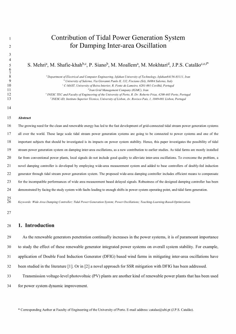
The global scheme for a practical DFIG based tidal stream power generation system is given by Fig. 1. In the 113

following, the detailed models for all sections of a TPGS are introduced. 114

115

5

116 117

Fig. 1. The global scheme for a practical DFIG based tidal stream power generation system 118 119

Tidal stream generators draw energy from water currents similar to the way that wind turbines draw energy from 120

air currents. Ordinary the tide speeds (i.e., spring and neap tides) move the Marine Current Turbine (MCT) [5]. Some 121

shorelines experience a semi-diurnal tide, two nearly equal high and low tides each day. Other locations experience 122

a diurnal tide, only one high and low tide each day. A "mixed tide"; two uneven tides a day, or one high and one low, 123

is also possible. The marine-currents are determined to start at 6 hours before high waters and to end 6 hours after 124

them. On this basis, deriving a simple and applied plan is not difficult for marine-current speeds, since tide factors 125

can be obtained as follows: 126

푉 = 푉 +(퐶 − 45)(푉 − 푉 )

95− 45

(1)

Where 푉 denotes the marine speed in m/s.퐶 represents the marine factor, 95 and 45 denote the average factors 127

of spring and neap tides, respectively.푉 and 푉 respectively represent the marine-current speed of the spring and 128

neap tides (for the area between France and England) [16]. The mechanical power of the considered MCT is 129

illustrated in Equation (2). 130

푃 = 휌 .퐴 .푉 .퐶 . (휆 ,훽 ) (2)

Where 휌 = 1025 kg/m denotes the seawater density, 퐴 represents the blade impact area in 푚 , and 퐶 131

denotes the power coefficient 퐶 of the MCT is given by 132

퐶 (휓 ,훽 ) = 푑 − 푑 .훽 − 푑 .훽 − 푑 푒푥푝 −

(3)

in which 133

1휓

=1

휆 + 푑 .훽−

푑훽 + 1

(4)

6

휆 =푅 .휔

푉

(5)

where 휔 is the blade angular velocity (rad/s), 푅 is the blade radius (m), 휆 is the tip speed ratio, 훽 is the 134

blade pitch angle (degrees), and 푑 − 푑 are the constant coefficients of power coefficient 퐶 of the MCT. Cut-in, 135

rate, and cut-out speeds of MCT are considered 1, 2.5, and 4 m/s, respectively. For the times that 푉 are more than 136

the nominal speed, the pitch-angle control loop starts decreasing the power of the MCT to the nominal one. Most of 137

the mathematical formulations used in an offshore wind farm can be employed in the marine current farm, because 138

the pitch-angle control loop, studied turbine, and mass-spring-damper models match with ones that are used in 139

offshore wind farm [17]. 140

141 Fig. 2. The considered two-inertia reduced-order tantamount mass-spring-damper. 142

143 144

The two-inertia reduced-order equivalent mass-spring damper model of the wind turbine directly coupled to the rotor 145

shaft of the wind DFIG is shown in Fig. 2 [18]. This model can also be applied to the equivalent mass-spring-damper 146

model of the marine current turbine coupled to the rotor shaft of the marine-current DFIG through an equivalent 147

gearbox (GB) whose effect can be properly included in this model. The equations of motion for the two-inertia 148

reduced-order marine current turbine model shown in Fig. 2 are expressed by [18]-[19]. 149

(2퐻 )푝(휔ℎ푡) = 푇 − 퐾 휃 − 퐷 휔 (6)

2퐻 푝 휔 = 퐾 휃 + 퐷 휔 − 푇 (7)

푝 휃 = 휔 (휔 −휔 ) (8)

where 휔 denotes the base angular speed. 퐻 and 퐻 represent inertias of tidal turbine and DFIG, respectively.퐾 150

and 퐷 denote the stiffness and damping coefficients between tidal turbine and DFIG, respectively. ω and θ 151

represent the angular speed and angle movement of each mass, respectively. 푇 denotes electromagnetic torque [19]. 152

7

2.2. Tidal DFIG 153

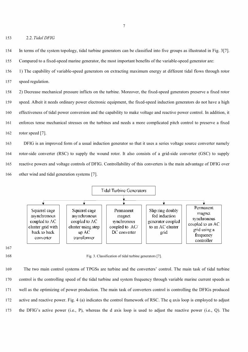
In terms of the system topology, tidal turbine generators can be classified into five groups as illustrated in Fig. 3[7]. 154

Compared to a fixed-speed marine generator, the most important benefits of the variable-speed generator are: 155

1) The capability of variable-speed generators on extracting maximum energy at different tidal flows through rotor 156

speed regulation. 157

2) Decrease mechanical pressure inflicts on the turbine. Moreover, the fixed-speed generators preserve a fixed rotor 158

speed. Albeit it needs ordinary power electronic equipment, the fixed-speed induction generators do not have a high 159

effectiveness of tidal power conversion and the capability to make voltage and reactive power control. In addition, it 160

enforces tense mechanical stresses on the turbines and needs a more complicated pitch control to preserve a fixed 161

rotor speed [7]. 162

DFIG is an improved form of a usual induction generator so that it uses a series voltage source converter namely 163

rotor-side converter (RSC) to supply the wound rotor. It also consists of a grid-side converter (GSC) to supply 164

reactive powers and voltage controls of DFIG. Controllability of this converters is the main advantage of DFIG over 165

other wind and tidal generation systems [7]. 166

167

Fig. 3. Classification of tidal turbine generators [7]. 168

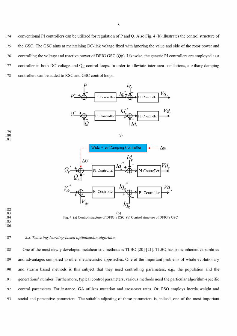
The two main control systems of TPGSs are turbine and the converters’ control. The main task of tidal turbine 169

control is the controlling speed of the tidal turbine and system frequency through variable marine current speeds as 170

well as the optimizing of power production. The main task of converters control is controlling the DFIGs produced 171

active and reactive power. Fig. 4 (a) indicates the control framework of RSC. The q axis loop is employed to adjust 172

the DFIG’s active power (i.e., P), whereas the d axis loop is used to adjust the reactive power (i.e., Q). The 173

8

conventional PI controllers can be utilized for regulation of P and Q. Also Fig. 4 (b) illustrates the control structure of 174

the GSC. The GSC aims at maintaining DC-link voltage fixed with ignoring the value and side of the rotor power and 175

controlling the voltage and reactive power of DFIG GSC (Qg). Likewise, the generic PI controllers are employed as a 176

controller in both DC voltage and Qg control loops. In order to alleviate inter-area oscillations, auxiliary damping 177

controllers can be added to RSC and GSC control loops. 178

*P

*rId

*rIq

Q

*Q

P

rId

rIq

rVd

rVq

179 (a) 180 181

*gQ

*gIq

*gId

dcV

*dcV

gQ

gIq

gId

gVq

gVd

U

182 (b) 183

Fig. 4. (a) Control structure of DFIG’s RSC, (b) Control structure of DFIG’s GSC 184 185 186

2.3. Teaching-learning-based optimization algorithm 187

One of the most newly developed metaheuristic methods is TLBO [20]-[21]. TLBO has some inherent capabilities 188

and advantages compared to other metaheuristic approaches. One of the important problems of whole evolutionary 189

and swarm based methods is this subject that they need controlling parameters, e.g., the population and the 190

generations’ number. Furthermore, typical control parameters, various methods need the particular algorithm-specific 191

control parameters. For instance, GA utilizes mutation and crossover rates. Or, PSO employs inertia weight and 192

social and perceptive parameters. The suitable adjusting of these parameters is, indeed, one of the most important 193

9

problems of evolutionary and swarm based methods. But unlike the mentioned algorithms, TLBO needs no 194

algorithm-specific parameters [20].This is one of the main benefits of TLBO compared to other metaheuristic 195

approaches because common control parameters are joint in solving each population-based optimization methods; 196

algorithm-specific parameters are particular to that method and various methods have various particular parameters 197

to control. TLBO has many similarities to evolutionary algorithms (EAs): an initial population is randomly selected, 198

moving on the way to the teacher and classmates is comparable to mutation operator in EA, and selection is based on 199

comparing two solutions in which the better one always survives [22]. 200

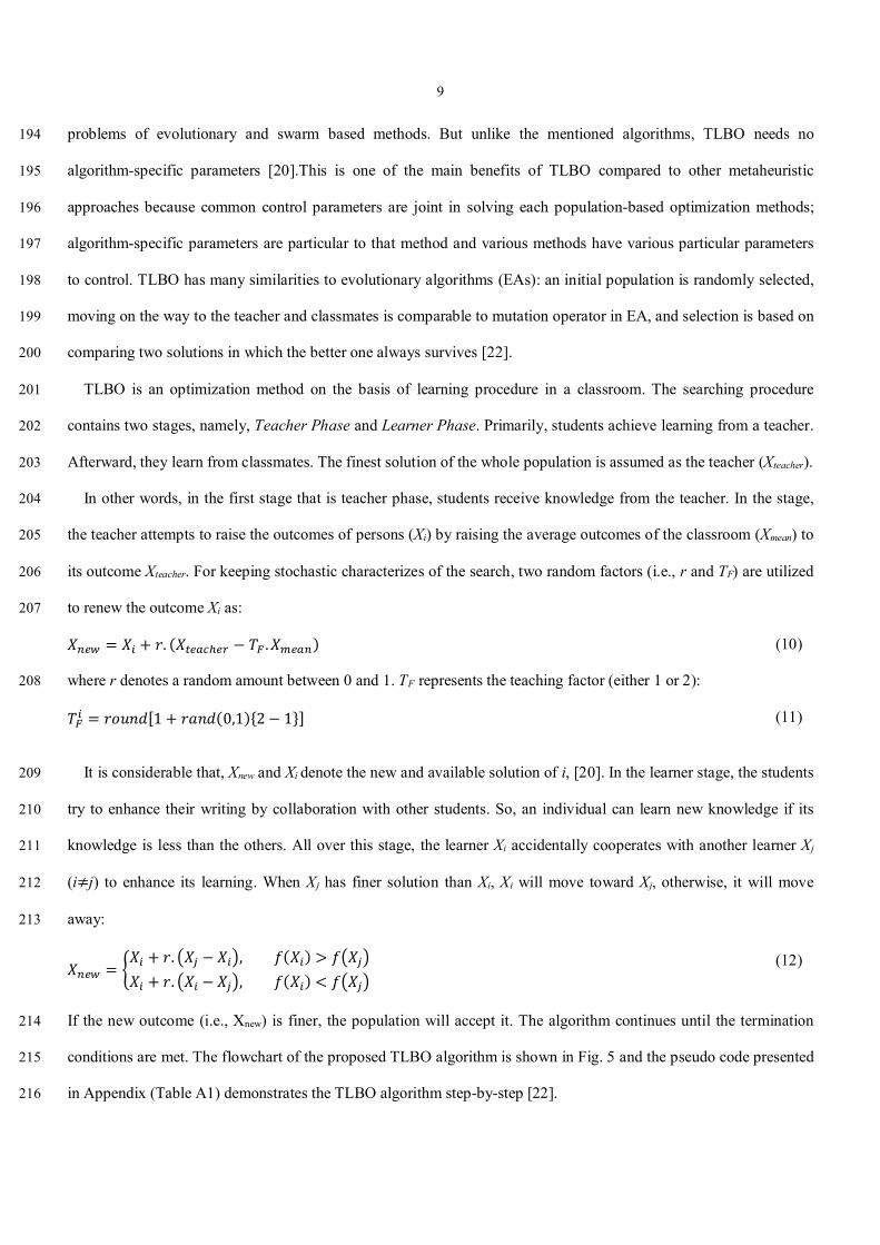
TLBO is an optimization method on the basis of learning procedure in a classroom. The searching procedure 201

contains two stages, namely, Teacher Phase and Learner Phase. Primarily, students achieve learning from a teacher. 202

Afterward, they learn from classmates. The finest solution of the whole population is assumed as the teacher (Xteacher). 203

In other words, in the first stage that is teacher phase, students receive knowledge from the teacher. In the stage, 204

the teacher attempts to raise the outcomes of persons (Xi) by raising the average outcomes of the classroom (Xmean) to 205

its outcome Xteacher. For keeping stochastic characterizes of the search, two random factors (i.e., r and TF) are utilized 206

to renew the outcome Xi as: 207

푋 = 푋 + 푟. (푋 − 푇 .푋 ) (10)

where r denotes a random amount between 0 and 1. TF represents the teaching factor (either 1 or 2): 208

푇 = 푟표푢푛푑[1 + 푟푎푛푑(0,1)2− 1] (11)

It is considerable that, Xnew and Xi denote the new and available solution of i, [20]. In the learner stage, the students 209

try to enhance their writing by collaboration with other students. So, an individual can learn new knowledge if its 210

knowledge is less than the others. All over this stage, the learner Xi accidentally cooperates with another learner Xj 211

(i≠j) to enhance its learning. When Xj has finer solution than Xi, Xi will move toward Xj, otherwise, it will move 212

away: 213

푋 =푋 + 푟. 푋 − 푋 , 푓(푋 ) > 푓 푋푋 + 푟. 푋 − 푋 , 푓(푋 ) < 푓 푋

(12)

If the new outcome (i.e., Xnew) is finer, the population will accept it. The algorithm continues until the termination 214

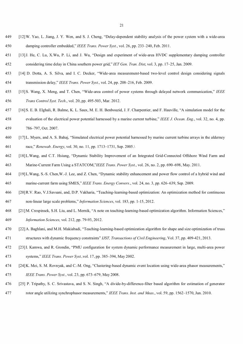
conditions are met. The flowchart of the proposed TLBO algorithm is shown in Fig. 5 and the pseudo code presented 215

in Appendix (Table A1) demonstrates the TLBO algorithm step-by-step [22]. 216

10

217

Fig. 5. Flowchart of the proposed TLBO algorithm 218

3. Results and Discussion 219 220

3.1. The Studied Power System 221

Because the main purpose of this paper is about damping of inter area fluctuations, the system chosen for case 222

study must be a large power system with multiple machines and several areas. So, in this paper the well-known three 223

area - six machine power system is used in this section as an example to validate the performance of the proposed 224

11

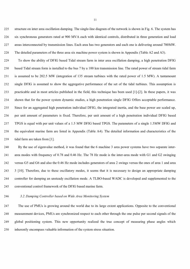
structure on inter area oscillation damping. The single-line diagram of the network is shown in Fig. 6. The system has 225

six synchronous generators rated at 900 MVA each with identical controls, distributed in three generation and load 226

areas interconnected by transmission lines. Each area has two generators and each one is delivering around 700MW. 227

The detailed parameters of the three area six machine power system is shown in Appendix (Table A2 and A3). 228

To show the ability of DFIG based Tidal stream farm in inter area oscillation damping, a high penetration DFIG 229

based Tidal stream form is installed to the bus 7 by a 100 km transmission line. The rated power of stream tidal farm 230

is assumed to be 202.5 MW (integration of 135 stream turbines with the rated power of 1.5 MW). A tantamount 231

single DFIG is assumed to show the aggregative performance of the set of the tidal turbines. This assumption is 232

practicable and in most articles published in the field, this technique has been used [1]-[2]. In these papers, it was 233

shown that for the power system dynamic studies, a high penetration single DFIG Offers acceptable performance. 234

Since for an aggregated high penetration individual DFIG, the integrated inertia, and the base power are scaled up, 235

per unit amount of parameters is fixed. Therefore, per unit amount of a high penetration individual DFIG based 236

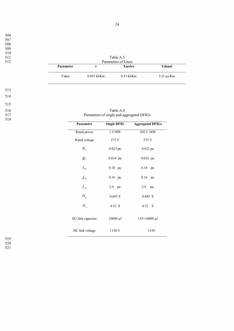
TPGS is equal with per unit values of a 1.5 MW DFIG based TPGS. The parameters of a single 1.5MW DFIG and 237

the equivalent marine farm are listed in Appendix (Table A4). The detailed information and characteristics of the 238

tidal farm are taken from [1]. 239

By the use of eigenvalue method, it was found that the 6 machine 3 area power systems have two separate inter-240

area modes with frequency of 0.78 and 0.46 Hz. The 78 Hz mode is the inter-area mode with G1 and G2 swinging 241

versus G5 and G6 and also the 0.46 Hz mode includes generators of area 2 swings versus the ones of area 1 and area 242

3 [10]. Therefore, due to these oscillatory modes, it seems that it is necessary to design an appropriate damping 243

controller for damping an unsteady oscillation mode. A TLBO-based WADC is developed and supplemented to the 244

conventional control framework of the DFIG based marine farm. 245

3.2. Damping Controller based on Wide Area Monitoring System 246

The use of PMUs is growing around the world due to its large extent applications. Opposite to the conventional 247

measurement devices, PMUs are synchronized respect to each other through the one pulse per second signals of the 248

global positioning system. This new opportunity realized the true concept of measuring phase angles which 249

inherently encompass valuable information of the system stress situation. 250

12

A WAMS is required to gather the PMUs’ data which is sent from designated places in the power system and 251

stored in a data storage system each 100 milliseconds. 252

1

5

61G

2

7L7C

7 8

9L9C

9 31110 3G

42G

4G

1L

2L

12 145G

136G 15

15L

PMU

PMU

PMU

DFIG

MW5.20216

253 Fig. 6. The considered power system with a DFIG marine farm. 254

255 One of the most practical applications of WAMS is oscillation damping which highly depends on the number and 256

location of PMUs placed on the grid. In order to oscillation damping, it seems that a definite number of PMUs will 257

meet the objective where the places of PMUs are chosen properly. This claim is proved by the numerical studies 258

provided in the following. The mentioned issue is intended by the authors for future work whereas some pioneering 259

research is currently available [23]. 260

A local damping controller is not indeed able to access to the oscillation signals while wide-area modal keep being 261

observable. On the contrary, WAMS application makes it possible to achieve global inter-area oscillation information 262

to apply to the damping controller. The most important contributing factor in the efficient behavior of WADC is to 263

feed the feedback signal delays to the controller; whereas, the local damping controller does not have this concern. 264

Obviously, WADC and local controller structure design are basically different due to the difference of their input 265

signals. WADC can alleviate multi-mode fluctuations. This capability is indicated by multi-band controllers which 266

each exerts its own global input signal to damp one of the oscillation modes. But, local damping controllers have 267

only one band to alleviate an oscillation mode. 268

13

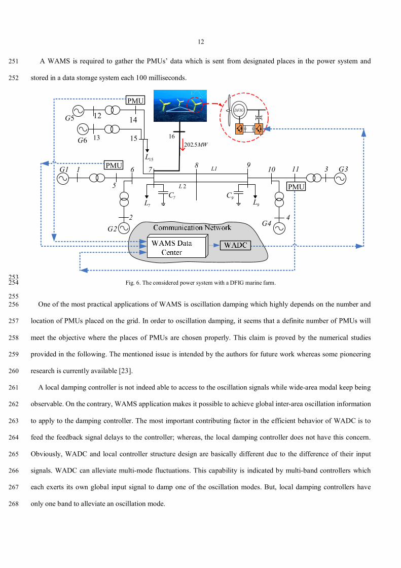
Since the considered system includes two inter-area modes, a two-band controller is employed as illustrated in Fig. 269

7. Band controllers are denoted by WADC1 and WADC2 and the whole unit is recognized by WADC. 270

3113

5115

1W

2W

1Vq

2Vq output

271 Fig. 7. The considered two-band WADC. 272

273

Apparently, to alleviate multi-mode oscillations, it is essential to have two additional signals including both modes 274

of oscillation. Any type of input signals which has suitable modal observability of inter-area oscillations may be 275

utilized, e.g., the tie line power, the frequency difference of areas, and angle difference of areas. 276

Commonly, PMUs receive the three-phase voltage and current in a sinusoidal waveform. Afterward, the phasor 277

values are obtained by converting the sampled digital data, and will be sent to the system control center. 278

Even though the PMU’s frequency and the rate of change depend on measuring the voltage, a number of methods 279

have been reported to compute the generator’s speed via local PMU measurements [24]-[26]. 280

Frequency indeed has a crucial role for the system stability and balance between generations and loads. Frequency 281

(or rotor speed) and the rates of change can be employed as the damping controller feedback signal [1]-[2] and [10]. 282

On this basis, it is assumed that PMUs located on high voltage buses (connected to G1, G3, and G5) where 283

3113 - and 5115 - are considered as global feedback signals. 15 and 13 are applied as the input 284

of WADC1 and WADC2 respectively to alleviate the inter-area oscillation modes 1 (0.78 Hz) and 2 (0.46 Hz) 285

correspondingly. As shown in Fig. 7, the output of WADC is weighted of both modes as indicated by equation (9). 286

2211 VqWVqWoutput (13)

where, W1 and W2 considered as weighting factors which obtained from the Prony analysis inversely proportional to 287

normalize damping ratio of their main mode (W1=1.15, W2=1) [10]. The WADC output is lastly used for modulation 288

of the DFIG’s reactive power loop. 289

Time synchronized data gathering and sending by the time-stamped PMUs makes the communication latency 290

computable if the local times of controller location are accessible through devoted GPS equipment. 291

14

The entire latency of transferred data can be computed by comparing the local time at the controller and the instant 292

of origin at the PMUs’ location [27]. It is necessary to note that if the controlled equipment is far from the controller, 293

the transmitting time of the commands is also considered. Due to the uncertainty of the communication system, the 294

latency does not get fixed completely. 295

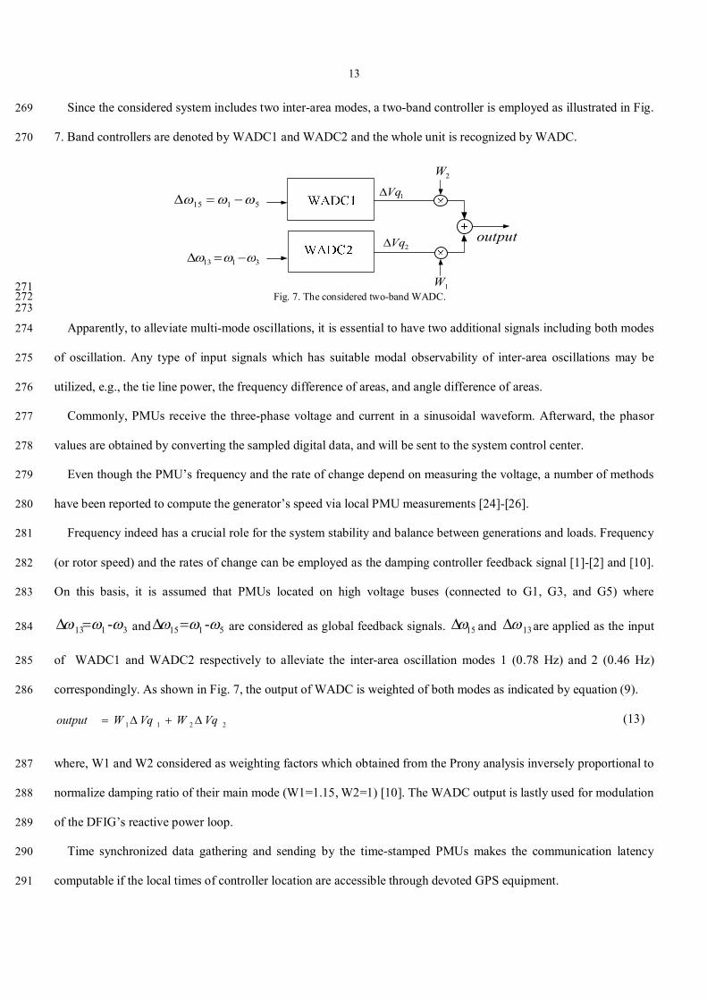
To evaluate the effects of time delay, an ideal designed WADC is examined in this study where the feedback 296

signal has several levels of time delay. As shown in Fig. 8, the total latency includes the sum of a fixed value and a 297

random number, i.e., 300 ±rand(50) milliseconds where the time delay variable is applied randomly. 298

299 Fig. 8. Random time delay of the remote feedback signal. 300

301 302

Here the tendency is to design a WADC, called delay-compensated WADC, in order to compensate for the 303

destructive effects resulted from the time delays. To meet this end, an additional input signal that represents the 304

latency of feedback signal is required to feed the DFIGs location to the damping controller. The parameter of the 305

time delay is implemented to the simulation setup throughout the design procedure and then the TLBO algorithm 306

optimizes the controller parameters. In this method, parameters of lead-lag compensator are adjusted, hence the phase 307

shifts between speed deviation and resulted electrical damping torque are compensated, and the adverse effects of 308

latency are also lessened. 309

300 ± rand (100) ms latencies in remote feedback signals are taken into account to design the latency-compensated 310

WADC. The final values of the WADC parameters are presented in Table I. 311

312

TABLE I 313 Parameters of Latency-Compensated WADCs 314

315 Type K TW T1 T2 T3 T4 min & max

WADC1 38 2 0.018 2 0.008 0.001 ±0.1

WADC2 33 2 2.1 0.001 2 0.001 ±0.1

316

0 5 10 15 20 25 30

0.2

0.3

0.4

Time (s)

varia

ble

time

dela

y (s

)

15

317

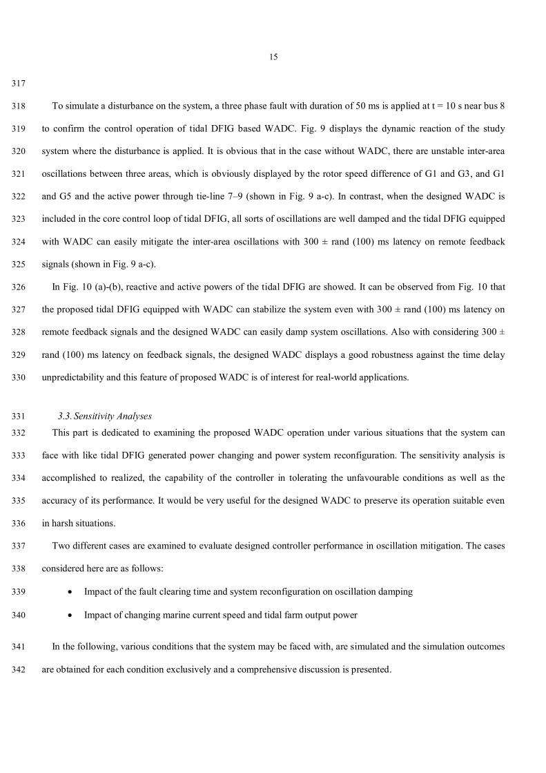
To simulate a disturbance on the system, a three phase fault with duration of 50 ms is applied at t = 10 s near bus 8 318

to confirm the control operation of tidal DFIG based WADC. Fig. 9 displays the dynamic reaction of the study 319

system where the disturbance is applied. It is obvious that in the case without WADC, there are unstable inter-area 320

oscillations between three areas, which is obviously displayed by the rotor speed difference of G1 and G3, and G1 321

and G5 and the active power through tie-line 7–9 (shown in Fig. 9 a-c). In contrast, when the designed WADC is 322

included in the core control loop of tidal DFIG, all sorts of oscillations are well damped and the tidal DFIG equipped 323

with WADC can easily mitigate the inter-area oscillations with 300 ± rand (100) ms latency on remote feedback 324

signals (shown in Fig. 9 a-c). 325

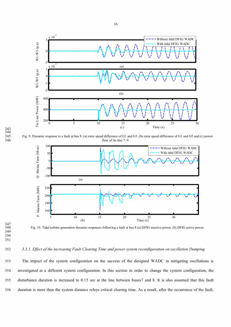
In Fig. 10 (a)-(b), reactive and active powers of the tidal DFIG are showed. It can be observed from Fig. 10 that 326

the proposed tidal DFIG equipped with WADC can stabilize the system even with 300 ± rand (100) ms latency on 327

remote feedback signals and the designed WADC can easily damp system oscillations. Also with considering 300 ± 328

rand (100) ms latency on feedback signals, the designed WADC displays a good robustness against the time delay 329

unpredictability and this feature of proposed WADC is of interest for real-world applications. 330

3.3. Sensitivity Analyses 331

This part is dedicated to examining the proposed WADC operation under various situations that the system can 332

face with like tidal DFIG generated power changing and power system reconfiguration. The sensitivity analysis is 333

accomplished to realized, the capability of the controller in tolerating the unfavourable conditions as well as the 334

accuracy of its performance. It would be very useful for the designed WADC to preserve its operation suitable even 335

in harsh situations. 336

Two different cases are examined to evaluate designed controller performance in oscillation mitigation. The cases 337

considered here are as follows: 338

Impact of the fault clearing time and system reconfiguration on oscillation damping 339

Impact of changing marine current speed and tidal farm output power 340

In the following, various conditions that the system may be faced with, are simulated and the simulation outcomes 341

are obtained for each condition exclusively and a comprehensive discussion is presented. 342

16

343 344

Fig. 9. Dynamic response to a fault at bus 8: (a) rotor speed difference of G1 and G3, (b) rotor speed difference of G1 and G5 and (c) power 345 flow of tie-line 7–9. 346

347 Fig. 10. Tidal turbine generation dynamic responses following a fault at bus 8 (a) DFIG reactive power, (b) DFIG active power. 348

349 350

351

3.3.1. Effect of the increasing Fault Clearing Time and power system reconfiguration on oscillation Damping 352

The impact of the system configuration on the success of the designed WADC in mitigating oscillations is 353

investigated at a different system configuration. In this section in order to change the system configuration, the 354

disturbance duration is increased to 0.15 sec at the line between buses7 and 8. It is also assumed that this fault 355

duration is more than the system distance relays critical clearing time. As a result, after the occurrence of the fault, 356

-5

0

5x 10

-3

(a)

W1-

W3

(p.u

)

-2

-1

0

1x 10

-3

W1-

W5

(p.u

)

(b)

0 5 10 15 20 25 30200

400

600

(c) Time (s)Tie

Line

Pow

er (M

W)

Without tidal DFIG WADCWith tidal DFIG WADC

-100

-50

0

50

100

Q- M

arin

e Fa

rm (M

var)

(b) Time (s)5 10 15 20 25 30

160

180

200

220

P- M

arin

e Fa

rm (M

W)

(a)

Without tidal DFIG WADCWith tidal DFIG WADC

17

distance relay of the line between buses 7 and bus 8 responds to the fault with tripping this line. As a result of this 357

action, the line between bus 7 and 8 is switched off from the system and the system configuration will be changed. 358

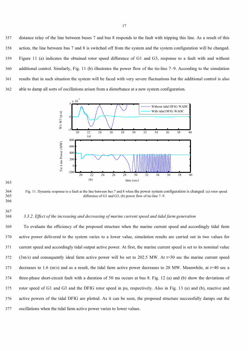
Figure 11 (a) indicates the obtained rotor speed difference of G1 and G3, response to a fault with and without 359

additional control. Similarly, Fig. 11 (b) illustrates the power flow of the tie-line 7–9. According to the simulation 360

results that in such situation the system will be faced with very severe fluctuations but the additional control is also 361

able to damp all sorts of oscillations arisen from a disturbance at a new system configuration. 362

363

Fig. 11. Dynamic response to a fault at the line between bus 7 and 8 when the power system configuration is changed: (a) rotor speed 364 difference of G1 and G3, (b) power flow of tie-line 7–9. 365

366

367 3.3.2. Effect of the increasing and decreasing of marine current speed and tidal farm generation 368

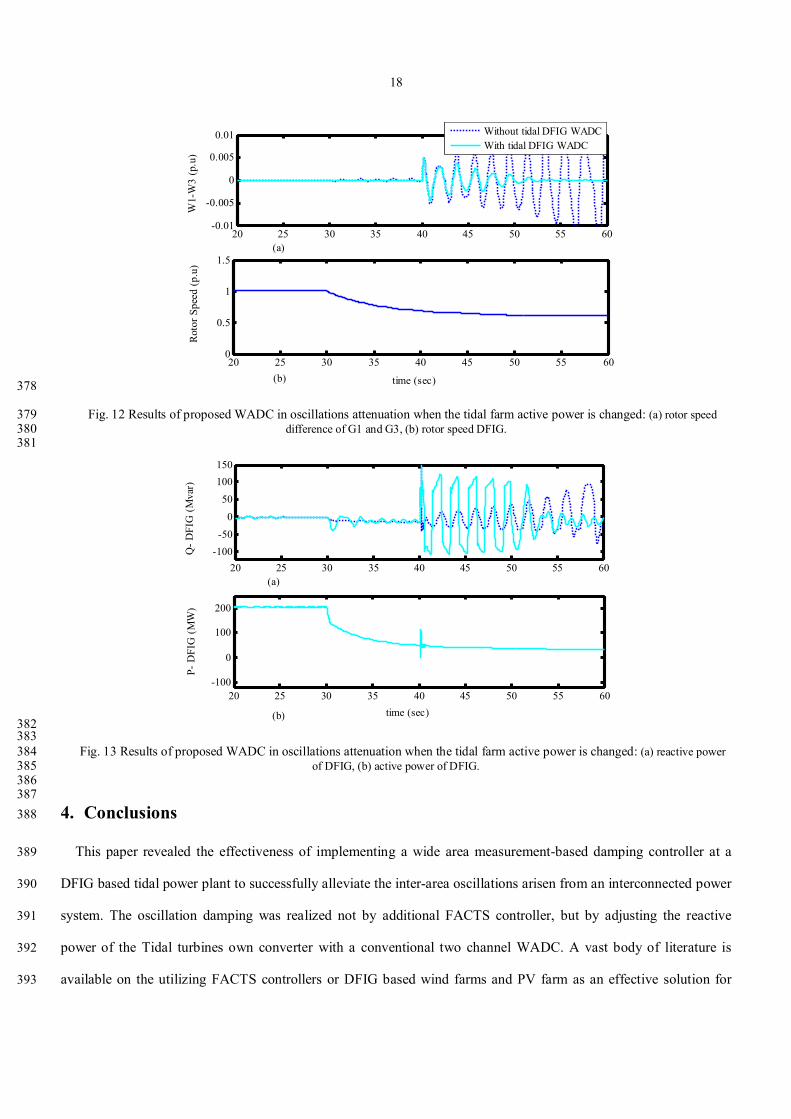
To evaluate the efficiency of the proposed structure when the marine current speed and accordingly tidal farm 369

active power delivered to the system varies to a lower value, simulation results are carried out in two values for 370

current speed and accordingly tidal output active power. At first, the marine current speed is set to its nominal value 371

(3m/s) and consequently ideal farm active power will be set to 202.5 MW. At t=30 sec the marine current speed 372

decreases to 1.6 (m/s) and as a result, the tidal farm active power decreases to 20 MW. Meanwhile, at t=40 sec a 373

three-phase short-circuit fault with a duration of 50 ms occurs at bus 8. Fig. 12 (a) and (b) show the deviations of 374

rotor speed of G1 and G3 and the DFIG rotor speed in pu, respectively. Also in Fig. 13 (a) and (b), reactive and 375

active powers of the tidal DFIG are plotted. As it can be seen, the proposed structure successfully damps out the 376

oscillations when the tidal farm active power varies to lower values. 377

20 22 24 26 28 30 32 34 36 38 40-5

0

5x 10

-3

W1-

W3

(p.u

)

20 22 24 26 28 30 32 34 36 38 40-200

0

200

400

600

800

time (sec)

Tie

Line

Pow

er (M

W)

Without tidal DFIG WADCWith tidal DFIG WADC

(a)

(b)

18

378

Fig. 12 Results of proposed WADC in oscillations attenuation when the tidal farm active power is changed: (a) rotor speed 379 difference of G1 and G3, (b) rotor speed DFIG. 380

381

382 383

Fig. 13 Results of proposed WADC in oscillations attenuation when the tidal farm active power is changed: (a) reactive power 384 of DFIG, (b) active power of DFIG. 385

386 387

4. Conclusions 388

This paper revealed the effectiveness of implementing a wide area measurement-based damping controller at a 389

DFIG based tidal power plant to successfully alleviate the inter-area oscillations arisen from an interconnected power 390

system. The oscillation damping was realized not by additional FACTS controller, but by adjusting the reactive 391

power of the Tidal turbines own converter with a conventional two channel WADC. A vast body of literature is 392

available on the utilizing FACTS controllers or DFIG based wind farms and PV farm as an effective solution for 393

20 25 30 35 40 45 50 55 60-0.01

-0.005

0

0.005

0.01

W1-

W3

(p.u

)

Without tidal DFIG WADCWith tidal DFIG WADC

20 25 30 35 40 45 50 55 600

0.5

1

1.5

time (sec)

Roto

r Spe

ed (p

.u)

(a)

(b)

20 25 30 35 40 45 50 55 60-100

-500

50100150

Q- D

FIG

(Mva

r)

20 25 30 35 40 45 50 55 60-100

0

100

200

time (sec)

P- D

FIG

(MW

)

(b)

(a)

19

inter area oscillation damping. Mokhtari et al [1]-[2] have demonstrated the ability of DFIG based wind farm in 394

mitigating SSR and inter area oscillation. In both references [1]-[2], a PSO based conventional damping controller 395

has been designed and added to the main control loop of DFIG based wind farm to oscillation damping. Shah et all. 396

[3] have shown that a high penetration PV plant can be utilized for inter area oscillations attenuation. There are many 397

other manuscripts reporting the capability of all renewable power generation system for power system oscillation 398

mitigation. However, to the best knowledge of the authors, this is the first work that shows the ability of DFIG based 399

tidal stream farm to power system oscillation damping. Moreover, in all references cited above the renewable 400

generation systems are assumed to have constant produced power, while in this work the tidal farm produced power 401

changes are also considered in the simulation process. The Tidal farm auxiliary damping controllers implemented the 402

variable areas generator rotor speed variations as a feedback signal to produce the auxiliary damping signal and the 403

reactive power regulation of the DFIGs was utilized for inter-area fluctuations damping. The rotor speed deviations 404

for damping controller were obtained through wide-area information due to the utilization of PMUs dispersed over 405

the network. The TLBO approach was used for best adjusting of the controller’s parameters and possible signal delay 406

of feedback signals on WAMS was considered for the controller design. It was properly showed that the designed 407

WADC operates suitably and displays excellent robustness against transmission time delay uncertainties. In addition, 408

the obtained results with sensitivity analyses indicated that the operation of the designed WADC is highly robust 409

against varying the fault duration time and power system operating point and tidal farm generation. With the rapidly 410

increasing application of DFIG based tidal farms and PMUs, designing WAMS based supplementary control for tidal 411

farms for power systems dynamic enhancement is necessary and needs many research activities. In this subject, the 412

most important issue is the coordinated design of DFIGs and other renewable power generation systems like voltage-413

level PV plants based on using WAMS technology and considering the time-varying communication system delays. 414

The subjects are open future research themes in the scope of renewable energy systems and smart transmission grids. 415

416

Acknowledgements 417

J.P.S. Catalão acknowledges FEDER funds through COMPETE 2020 and Portuguese funds through FCT, under 418

Projects FCOMP-01-0124-FEDER-020282 (Ref. PTDC/EEA-EEL/118519/2010), POCI-01-0145-FEDER-016434, 419

POCI-01-0145-FEDER-006961, UID/EEA/50014/2013, UID/CEC/50021/2013, and UID/EMS/00151/2013. Also, 420

20

the research leading to these results has received funding from the EU Seventh Framework Programme FP7/2007-421

2013 under grant agreement no. 309048 422

423

References 424

[1] M. Mokhtari, and F. Aminifar, “Toward wide-area oscillation control through doubly-fed induction generator wind 425

farms,”IEEE Transactions on Power Systems, vol. 53, pp. 876–883, Nov. 2014. 426

[2] M. Mokhtari, J. Khazaei, and D. Nazarpour, “Sub-synchronous resonance damping via doubly fed induction generator,” 427

Electrical Power and Energy Systems, vol. 29, pp. 2985 - 2992, Dec. 2013. 428

[3] R. Shah, N. Mithulananthan, and Kwang Y. Lee , “Large-Scale PV Plant With a Robust Controller Considering Power 429

Oscillation Damping,” IEEE Trans. Energy Conver., vol. 28, no. 1, pp. 106-116, Mar. 2013. 430

[4] R. Shah, N. Mithulananthan, and R.C.Bansal, “Oscillatory stability analysis with high penetrations of large-scale 431

photovoltaic generation,” Energy Conversion and Management, vol. 65, pp. 420–429, Jan 2013. 432

[5] J. M. González-Caballín, E. Álvarez, A. J. Guttiérrez-Trashorras, A. Navarro-Manso, J. Fernández, E. Blanco, “Tidal current 433

energy potential assessment by a two dimensional computational fluid dynamics model: The case of Avilés port (Spain),” 434

Energy Conversion and Management, vol. 119, pp. 239-245, Jul. 2016. 435

[6] A. Vazquez, G. Iglesias, “A holistic method for selecting tidal stream energy hotspots under technical, economic and 436

functional constraints” Energy Conversion and Management, vol. 117, pp. 420-430, Jun. 2016. 437

[7] J. Khan, C. Morton, and A. Rao, “Electrical power connectors for marine energy systems,” Tech. Rep. 20490-21-00 Rep-1, 438

2011, prepared by Powertech Labs Inc. for Natural Resources Canada (NRCan). 439

[8] K.R. Padiyar, V. Swayam, ‘‘ Prakash tuning and performance evaluation of damping controller for a STATCOM, 440

International Journal of Electrical Power & Energy Systems, Vol. 25, no. 2, pp. 155–166. Feb. 2003. 441

[9] X. Xie, J. Xiao, C. Lu, and Y. Han, “Wide-area stability control for damping interarea oscillations of interconnected power 442

systems,” IET Gen. Tran. Dis, vol. 153, pp. 507-514, Sept. 2006. 443

[10] M. Mokhtari, F. Aminifar, D. Nazarpour, and S. Golshannavaz, “Wide-area power oscillation damping with a Fuzzy 444

controller compensating the continuous communication delays” IEEE Trans. Power Syst., vol. 28, pp. 1997-2005, May 445

2013. 446

[11] N. R. Chaudhuri, S. Ray, R. Majumder, and B. Chaudhuri, “A new approach to continuous latency compensation with 447

adaptive phasor power oscillation damping controller (POD),” IEEE Trans. Power Syst., vol. 25, pp. 939–946, May 2010. 448

21

[12] W. Yao, L. Jiang, J. Y. Wen, and S. J. Cheng, “Delay-dependent stability analysis of the power system with a wide-area 449

damping controller embedded,” IEEE Trans. Power Syst., vol. 26, pp. 233–240, Feb. 2011. 450

[13] J. He, C. Lu, X.Wu, P. Li, and J. Wu, “Design and experiment of wide-area HVDC supplementary damping controller 451

considering time delay in China southern power grid,” IET Gen. Tran. Dist, vol. 3, pp. 17–25, Jan. 2009. 452

[14] D. Dotta, A. S. Silva, and I. C. Decker, “Wide-area measurement-based two-level control design considering signals 453

transmission delay,” IEEE Trans. Power Syst., vol. 24, pp. 208–216, Feb. 2009. 454

[15] S. Wang, X. Meng, and T. Chen, “Wide-area control of power systems through delayed network communication,” IEEE 455

Trans Control Syst. Tech., vol. 20, pp. 495-503, Mar. 2012. 456

[16] S. E. B. Elghali, R. Balme, K. L. Saux, M. E. H. Benbouzid, J. F. Charpentier, and F. Hauville, “A simulation model for the 457

evaluation of the electrical power potential harnessed by a marine current turbine,” IEEE J. Ocean. Eng., vol. 32, no. 4, pp. 458

786–797, Oct. 2007. 459

[17] L. Myers, and A. S. Bahaj, “Simulated electrical power potential harnessed by marine current turbine arrays in the alderney 460

race,” Renewab. Energy, vol. 30, no. 11, pp. 1713–1731, Sep. 2005.\ 461

[18] L.Wang, and C.T. Hsiung, “Dynamic Stability Improvement of an Integrated Grid-Connected Offshore Wind Farm and 462

Marine-Current Farm Using a STATCOM,”IEEE Trans. Power Syst., vol. 26, no. 2, pp. 690–698, May. 2011. 463

[19] L.Wang, S.-S. Chen,W.-J. Lee, and Z. Chen, “Dynamic stability enhancement and power flow control of a hybrid wind and 464

marine-current farm using SMES,” IEEE Trans. Energy Convers., vol. 24, no. 3, pp. 626–639, Sep. 2009. 465

[20] R.V. Rao, V.J.Savsani, and, D.P. Vakharia, “Teaching-learning-based optimization: An optimization method for continuous 466

non-linear large scale problems,” Information Sciences, vol. 183, pp. 1-15, 2012. 467

[21] M. Crespinsek, S.H. Liu, and L. Mernik, “A note on teaching-learning-based optimization algorithm. Information Sciences,” 468

Information Sciences, vol. 212, pp. 79-93, 2012. 469

[22] A. Baghlani, and M.H. Makiabadi, “Teaching-learning-based optimization algorithm for shape and size optimization of truss 470

structures with dynamic frequency constraints” IJST, Transactions of Civil Engineering, Vol. 37, pp. 409-421, 2013. 471

[23] I. Kamwa, and R. Grondin, “PMU configuration for system dynamic performance measurement in large, multi-area power 472

systems,” IEEE Trans. Power Syst.,vol. 17, pp. 385–394, May 2002. 473

[24] K. Mei, S. M. Rovnyak, and C.-M. Ong, “Clustering-based dynamic event location using wide-area phasor measurements,” 474

IEEE Trans. Power Syst., vol. 23, pp. 673–679, May 2008. 475

[25] P. Tripathy, S. C. Srivastava, and S. N. Singh, “A divide-by-difference-filter based algorithm for estimation of generator 476

rotor angle utilizing synchrophasor measurements,” IEEE Trans. Inst. and Meas., vol. 59, pp. 1562–1570, Jun. 2010. 477

22

[26] E. Ghahremani, and I. Kamwa, “Dynamic state estimation in power system by applying the extended Kalman filter with 478

unknown inputs to phasor measurements,” IEEE Trans. Power Syst., vol. 26, pp. 2556–2566, Nov. 2011. 479

[27] P. Korba, R. Segundo, A. Paice, B. Berggren, and R. Majumder, “Time delay compensation in power system control,” 480

European Union Patent, EP08 156 785, May. 2008. 481

482

23

Appendix 483 484 485

Table A1 486 Pseudo code of TLBO 487

488

489

490 491 492 493

Table A.2 494 Parameters of Generators 495

1G 2G 3G 4G 5G 6G

dx 8.1 8.1 8.1 8.1 8.1 8.1

dx 3 3 3 3 3 3

qx 7.1 7.1 7.1 7.1 7.1 7.1

doT 8 8 8 8 8 8

sr 003.0 003.0 003.0 003.0 003.0 003.0

fr 0006.0 0006.0 0006.0 0006.0 0006.0 0006.0

fx 1.0 1.0 1.0 1.0 1.0 1.0

H 5.6 5.6 5.6 5.6 5.6 5.6 496 497 498 499 500 501 502 503 504 505

24

506 507 508 509 510

Table A.3 511 Parameters of Lines 512

Parameter r Xseries Yshunt

Value 0.053 Ω/Km 0.53 Ω/Km 5.21 μs/Km

513 514

515 Table A.4 516

Parameters of single and aggregated DFIGs 517 518

Parameter Single DFIG Aggregated DFIGs

Rated power 1.5 MW 202.5 MW

Rated voltage 575 V 575 V

SR 0.023 pu 0.023 pu

rR' 0.016 pu 0.016 pu

lSL 0.18 pu 0.18 pu

lrL' 0.16 pu 0.16 pu

mL 2.9 pu 2.9 pu

gH 0.685 S 0.685 S

tH 4.32 S 4.32 S

DC-link capacitor 10000 µf 135×10000 µf

DC-link voltage 1150 V 1150

519 520 521