Contrast analysis

Citation for published version (APA):Haans, A. (2018). Contrast analysis: A tutorial. Practical Assessment, Research & Evaluation, 23(9), 1-21. [9].https://doi.org/10.7275/zeyh-j468

DOI:10.7275/zeyh-j468

Document status and date:Published: 01/01/2018

Document Version:Publisher’s PDF, also known as Version of Record (includes final page, issue and volume numbers)

Please check the document version of this publication:

• A submitted manuscript is the version of the article upon submission and before peer-review. There can beimportant differences between the submitted version and the official published version of record. Peopleinterested in the research are advised to contact the author for the final version of the publication, or visit theDOI to the publisher's website.• The final author version and the galley proof are versions of the publication after peer review.• The final published version features the final layout of the paper including the volume, issue and pagenumbers.Link to publication

General rightsCopyright and moral rights for the publications made accessible in the public portal are retained by the authors and/or other copyright ownersand it is a condition of accessing publications that users recognise and abide by the legal requirements associated with these rights.

• Users may download and print one copy of any publication from the public portal for the purpose of private study or research. • You may not further distribute the material or use it for any profit-making activity or commercial gain • You may freely distribute the URL identifying the publication in the public portal.

If the publication is distributed under the terms of Article 25fa of the Dutch Copyright Act, indicated by the “Taverne” license above, pleasefollow below link for the End User Agreement:www.tue.nl/taverne

Take down policyIf you believe that this document breaches copyright please contact us at:openaccess@tue.nlproviding details and we will investigate your claim.

Download date: 05. Apr. 2022

A peer-reviewed electronic journal.

Copyright is retained by the first or sole author, who grants right of first publication to Practical Assessment, Research & Evaluation. Permission is granted to distribute this article for nonprofit, educational purposes if it is copied in its entirety and the journal is credited. PARE has the right to authorize third party reproduction of this article in print, electronic and database forms.

Volume 23 Number 9, May 2018 ISSN 1531-7714

Contrast Analysis: A Tutorial Antal Haans, Eindhoven University of Technology

Contrast analysis is a relatively simple but effective statistical method for testing theoretical predictions about differences between group means against the empirical data. Despite its advantages, contrast analysis is hardly used to date, perhaps because it is not implemented in a convenient manner in many statistical software packages. This tutorial demonstrates how to conduct contrast analysis through the specification of the so-called L (the contrast or test matrix) and M matrix (the transformation matrix) as implemented in many statistical software packages, including SPSS and Stata. Through a series of carefully chosen examples, the main principles and applications of contrast analysis are explained for data obtained with between- and within-subject designs, and for designs that involve a combination of between- and within-subject factors (i.e., mixed designs). SPSS and Stata syntaxes as well as simple manual calculations are provided for both significance testing and contrast-relevant effect sizes (e.g., η2

alerting). Taken together, the reader is provided with a comprehensive and powerful toolbox to test all kinds of theoretical predictions about cell means against the empirical data.

The statistical analysis of empirical data serves a single function: to answer research questions about a population on the basis of observations from a sample. In experimental psychology, these questions usually involve specific theoretical predictions about differences between group or cell means. Researchers, however, do not always transform their research question into the proper statistical question, which, among other things, involves the application of the correct statistical method (Hand, 1994). Since any statistical test answers a specific question (also Haans, 2008), conducting an incorrect test results in what Hand (1994) called an error of the third kind: “giving the right answer to the wrong question” (p. 317).

To illustrate the prevalence of such Type III errors, consider the following example. A group of researchers wants to test a specific theory-driven explanation for the observation that student retention of the discussed materials decreases more or less linearly with the distance between the student and the teacher in the lecturing hall. This effect of seating location, the researchers theorized, could be explained by the decreasing frequency of eye contact over distance. To test this theoretical explanation, they conducted a 2

(teacher wearing sunglasses or not) by 4 (student sitting in first, second, third, or fourth row of the lecturing hall) between-subject experiment with performance on a subsequent retention test as the dependent variable. Their theoretical prediction is that seating location has a negative linear relation with retention, but only in the condition in which the teacher did not wear sunglasses. The rationale is that wearing sunglasses effectively decreases any effect of eye contact regardless of where in the classroom the student is located, so that no effect of seating location on retention is expected for these groups. The research questions thus are: Is their specific theory-based prediction supported by the data? And if so, how much of the empirical or observed variance associated with the experimental manipulations can be explained by the theory?

Assume that the researchers in our example consulted a standard textbook to determine how they should analyze their empirical data. Their textbook would most likely insist on using a factorial ANOVA in which differences between observed cell means are explained by two main effects and an interaction effect. Doing so, the researchers, as expected, found a

Practical Assessment, Research & Evaluation, Vol 23 No 9 Page 2 Haans, Contrast Analysis: A Tutorial statistically significant interaction between the seating location and sunglasses factors. This interaction effect signifies that the effect of seating location was indeed different with as compared to without the teacher wearing sunglasses. However, one should not be lured into making a Type III error: Neither the significant interaction effect, nor any of the main effects provide an answer to the researchers’ question of interest. The interaction effect in a 2 by 4 design has three degrees of freedom in the numerator of the F-test, and thus is an omnibus test. In contrast to focused tests (with a single degree of freedom in the numerator), omnibus tests are not directly informative regarding the observed pattern of the effect. There are multitudes of ways in which the effect of seating location may be different between the different levels of the Sunglasses factor. Yet, only one is predicted by our researchers’ theory. As a result, eyeballing a graph depicting observed group means in combination with conducting a series of post-hoc comparisons will be needed to validate whether the significant interaction is consistent with their expectations. None of these post-hoc analyses will answer directly the researchers’ question of interest, let alone be informative about the extent to which their theory was able to explain the observed or empirical differences between group means (i.e., as reflected in an effect size). Would it not be more fruitful if one could test theoretical expectations directly against the observed or empirical data?

One such method that allows researchers to test theory-driven expectations directly against empirically derived group or cells means is contrast analysis. Despite its clear advantages, contrast analysis is hardly used to date, not even when strong a priori hypotheses are available. Instead, researchers typically rely on factorial ANOVA as the conventional method for analyzing experimental designs—as if the technique is “some ‘Mt Everest’ that must be scaled just because ‘it is there’ “(Rosnow & Rosenthal, 1996; p. 254). The unpopularity of contrast analysis cannot be explained by it being a novel or complicated technique (Rosenthal, Rosnow, & Rubin, 2000). In fact, the mathematics behind are understandable even to researchers with a minimal background in statistics. According to Abelson (1964; cited in Rosenthal et al., 2000), the unpopularity of contrast analysis may well be explained by its simplicity: “One compelling line of explanation is that the statisticians do not regard the idea as mathematically very interesting (it is based on quite elementary statistical concepts) …” (p. ix). Simple

statistical techniques, however, often produce the most meaningful and robust results (Cohen, 1990).

Yet another compelling explanation for the unpopularity of contrast analysis is that the method is not implemented, at least not in a convenient point-and-click manner, in most statistical software packages. In for example SPSS, some contrasts (e.g., Helmert and linear contrasts) are implemented and accessible through the user interface of the various procedures, but these are generally of limited use when finding answers to theory-driven questions (i.e., only infrequently do these contrasts answer a researcher’s question of interest). Custom contrasts may be defined in the user interface window of the ONEWAY procedure, but they are not available for more complex designs (e.g., for designs that include a within-subject factor). To unleash the full power of contrast analysis, many statistical software packages require researchers to specify manually the so-called contrast or test matrix L and / or the transformation matrix M. In SPSS, this is done through the LMATRIX and MMATRIX subcommands of the General Linear Model (GLM) procedure (IBM Corp., 2013). In Stata, they can be specified in the MANOVATEST postestimation command of the MANOVA procedure (StataCorp LP, 2015).

In the present paper, I will demonstrate how to specify the L and M matrices to test a wide variety of focused questions in a simple and time efficient manner. First, I will discuss contrast analysis for hypothesis testing and effect size estimation in between-subject factorial designs. After that, I will discuss factorial designs with within-subject factors, and designs with a combination of between and within-subject factors (so-called mixed designs). The aim of the manuscript is to provide researchers with a toolbox to test a wide variety of theory-driven hypotheses on their own data. I will not discuss in detail the computations behind contrast analysis, and the interested reader is referred to, for example, Rosenthal and colleagues (2000) and Wiens and Nilsson (2017). The procedures and explanations provided are kept simple, and more advanced comments are provided in footnotes. In the examples below, I explain the procedure as it is implemented in SPSS. Explanations for Stata users are presented in annotated syntax or .do files. Stata and SPSS syntax files together with all example datasets are available to the reader as supplementary materials (see end note for download link).

Practical Assessment, Research & Evaluation, Vol 23 No 9 Page 3 Haans, Contrast Analysis: A Tutorial Contrast analysis in between-subject

designs

Single factor between-subject designs

In a single factor (or one-way) between-subject design each of n participants is assigned to one of the g levels of the single factor. Consider the following hypothetical example, which will be used throughout the subsequent sections: A group of environmental psychologists is interested in the relation between class room seating location and educational performance. As part of their investigations, the researchers conducted a between-subject experiment in which students of a particular course were randomly assigned to sit either on the first (i.e., closest to the teacher), second, third, or the fourth row of the lecturing hall throughout a course’s lectures. Students’ grades on the final exam were used as an indicator of their educational performance. The single factor is labeled Location, and consist of g = 4 levels: first row (coded with a 1), second row (coded with a 2), third row (coded with a 3), and the fourth row (coded with a 4). A total of n = 20 students participated in the experiment, each randomly assigned to one of the four conditions. Their exams grades are provided in Table 1; graded on a scale from 0 (poor) to 10 (perfect score).

A conventional one-way ANOVA on the data in Table 1 will tell the researchers what amount of variance in the data can be attributed to differences in seating location. The outcome of this test is reported in Figure 1. The total amount of variance in educational performance, or sum of squares (SS), is called SStotal. This is labeled SScorrected total in the output of SPSS (see Figure 1). Part of these individual differences in educational performance will be due to group membership, and thus the effect of the seating location manipulation. This variance is called SSmodel, and is labeled SScorrected model in the output of SPSS (see Figure 1). The variance not

explained by group membership is SSresidual (labeled SSerror

in SPSS), and includes variance due to individual differences in for example general intelligence, or due to individuals responding differently to the experimental manipulations. SStotal can thus be decomposed into two parts:

SStotal SSmodel SSresidual (1)

We find that the total amount of variance in the data is SStotal = 125, of which SSmodel = 85 can be explained by group membership, and SSresidual = 40 cannot (see Figure 1). The SSlocation provides the amount of variance observed to be associated with the manipulation of seating locations. Since seating location completely defines group membership in our single factor design SSmodel = SSlocation = 85.

The proportion of variance in educational performance that is observed to be associated with differential seating locations can be expressed in an effect size estimate called eta-squared or η2:

ηSSmodelSStotal

(2)

Differential seating locations can explain η2 = 85/125 = 68% of the variance in the data. The corresponding F-test provides F(3,16) = 11.3 and p < .001. In other words, the probability of finding the observed, or even larger differences between the groups, is smaller than 0.1% when no effect of seating location is present in the population of students; that is if the null hypothesis is true. This probability is smaller than what we usually find acceptable (p < .05), so we reject the null-hypothesis which states that the four groups do not differ in educational performance. In other words, the main effect of location is statistically significant. Since

Table 1. Data and group means (μg) for the single factor design.

Location Row 1 Row 2 Row 3 Row 4

5  7  5  16  9  4  37  8  6  48  5  7  29  6  8  0

μ1= 7 μ2= 7 μ3 = 6 μ4 = 2

Figure 1. Excerpt of the SPSS output of a conventional between-subject ANOVA on the data of the 1 by 4 design in Table 1.

Practical Assessment, Research & Evaluation, Vol 23 No 9 Page 4 Haans, Contrast Analysis: A Tutorial the F-test for the main effect of seating location is an omnibus test—the degrees of freedom of the nominator (dflocation) are larger than one—the main effect alone is not informative about which of the groups of students are statistically different from each other on their educational performance. As a result additional post-hoc analyses are required to explore in more detail the differences between groups.

The conventional ANOVA answers the question of whether a student’s seating location affects educational performance, and to what extent. Interesting as such an empirical fact at times may be, the more interesting scientific questions are aimed at confirming or refuting theories that explain such empirical observations. Such questions require that focused and theory-driven expectations about differences between group means are tested against the empirical data. In the case of a between-subject design, these theoretical predications can be described by a row vector L consisting of a series contrast weights (lg), one for each of the g groups in the design. To test a theoretical prediction against the empirically derived group means, these contrast weights have to be specified in the so-called LMATRIX subcommand of the GLM procedure. The examples below illustrate how this is done for a variety of theory-driven hypotheses on data in Table 1.

Example 1: A first-row effect? One psychological theory of which the researchers expect it can explain the observed effect of seating location on education performance is based on social influence. This theory posits that all teachers have an invisible aura of power that submits all first-row students to a state of undivided attention. This theory would predict that the students sitting first-row will, on average, have higher grades than students sitting in rows two, three, and four. To test this theory against the data, the following focused question is to be asked: Is the average grade of students sitting in the first row higher than the average grade of students sitting in the other three rows? The following relation between the group means is thus expected: H1: μ1 > (μ2 + μ3 + μ4)/3. This can be rewritten as: μ1 ‒ 1/3μ2 ‒ 1/3μ3 ‒ 1/3μ4 > 0. The multipliers or weights in this equation

1 In ANOVA calculations, it is common to use, not the group means (μg), but the effects of group membership (Φg) which are 

relative to the grand mean or intercept (μ.), so that μg = μ. + Φg. The alternative hypothesis of the contrast in Example 1 can thus be rewritten as H1: 1(μ. + Φ1) – 1/3(μ. + Φ2) – 1/3(μ. + Φ3) – 1/3(μ. + Φ4) > 0, or H1: 0μ. + 1Φ1 – 1/3Φ2 – 1/3Φ3 – 1/3Φ4 > 0. The weight for the grand mean or intercept (μ.) thus is l0 = 0 for this theoretical prediction. 

2 Copying and pasting the syntax in this manuscript into to the SPSS syntax editor may in some cases result in error messages. SPSS does not always recognize the double quotation marks correctly when syntax is copied and pasted from external sources. 

are the contrast weights (lg) that describe this focused question: l1 = 1, l2 = -1/3, l3 = -1/3, and l4 = -1/3. This set of weights can also be written as a row vector L = [1 -1/3 -1/3 -1/3]. The precise order of the contrast weights is dependent on how the levels of the factor are coded in your data set: The first contrast weight is for the first level (g = 1), the second for the second level (g = 2), etc. Questions are: Is this theoretical expectation supported by the data, and if so, to what extent?

To perform the necessary analyses, one has to provide SPSS with the set of contrast weights that describes our theoretical hypothesis. For this purpose the following syntax needs to be specified in the SPSS syntax editor:

GLM grade BY location /LMATRIX = “Example 1: First row effect?” location 1 -1/3 -1/3 -1/3 intercept 0 /DESIGN = location.

The first line of the syntax specifies the dependent variable Grade and the independent variable or factor Location to be used in the General Linear Model (GLM) procedure. The LMATRIX subcommand is used to define our focused question or contrast. First, one can use quotation marks to provide a label for one’s focused question (i.e., “Example 1: First row effect?”). Second, the set of contrast weights for each level of the Location factor are provided. Finally, the weight of the so-called intercept or grand mean (l0) is provided. It can be calculated by taking the sum of the four weights (lg) specified in the contrast vector L: l0 = ∑lg. This value is usually zero1. Finally, the DESIGN subcommand specifies the structure of the experimental design which in this example involves a single factor called Location. Instead of typing in the complete syntax, you can use the SPSS graphical user interface to set up a conventional ANOVA, paste the instructions to the syntax editor, and add the LMATRIX subcommand2. Finally select the syntax and press run.

Practical Assessment, Research & Evaluation, Vol 23 No 9 Page 5 Haans, Contrast Analysis: A Tutorial

In the SPSS output, you will find two tables under the heading Custom Hypothesis Tests (see Figure 2). The contrast results table provides the contrast estimate (C) for this focused question, its standard error and 95% confidence interval, and the statistical significance of the hypothesis test (i.e., the p-value). The Contrast Results table provides C = 2.0 with a 95% confidence interval of 0.3 to 3.7. The contrast estimate C is obtained by taking the sum of all observed group means (μg) weighted by their contrast weights (lg): C = 1μ1 ‒ 1/3μ2 ‒ 1/3μ3 ‒ 1/3μ4 = 1×7 ‒ 1/3×7 ‒ 1/3× 6 ‒ 1/3×2 = 2.0. This C estimate directly answers our focused question: The difference between first row students and the other students is 2.0 grade points on average. The C-estimate is best interpreted as an unstandardized effect size. The larger the C is, the better the theory is supported by the empirical data. However, since it is unstandardized—meaning that it, amongst other things, depends on the exam grading scale—this result cannot always be compared directly with that of other studies.

This C = 2.0 can subsequently be tested against the null-hypothesis stating that the average grade of first-row students is identical to the average grade of all other students in the population. This null-hypothesis, thus, is: H0: C = 1μ1 ‒ 1/3μ2 ‒ 1/3μ3 ‒ 1/3μ4 = 0 (the hypothesized value as it is labeled in Figure 2). The statistical significance of this test is p = .026. We thus reject H0 in favor of H1. One should, however, always carefully check the sign of the contrast estimate C as a similar p-value would be found with C = -2.0 (which would indicate the opposite of the expected first row

effect). The results of the hypothesis test, now with the usual statistics of the F-test, are once more provided in the Test Results table: F(1,16) = 6.0 and p = .026 (see Figure 2). Notice that the degrees of freedom of the nominator of the F-test equal one. Testing a specific theoretical prediction against the data thus involves a focused rather than omnibus test. Focused tests are directly meaningful without any further need for post-hoc analysis.

More interesting is the question of how much of the empirical or observed variance associated with differential seating locations can be explained by the theory. In other words, how much of the SSmodel = 85 obtained with the conventional ANOVA (labeled SScorrected model in Figure 1) can the theory account for? The answer is provided by SScontrast in Figure 2 which reflects variance in educational performance explained by our theory. Since no theory will perfectly predict all the empirical differences between the groups, SScontrast will be smaller than SSmodel. Following Rosenthal and colleagues (2000), we will label the difference as SSnoncontrast which reflects the amount of between-group variance that the theory cannot explain:

model contrast noncontrast (3)

We find that SScontrast = 15 (see Figure 2), so that SSnoncontrast = 85 – 15 = 70. Standardized effect sizes may be calculated using the η2 introduced in Equation 2. Dividing SScontrast by the SStotal as obtained with a conventional ANOVA (labeled SScorrected total in the SPSS output in Figure 1) provides an estimate of the proportion of variance in educational performance that was explained by the theory:

η contrast

total (4)

Using this equation, we find that η2 = 15/125 = 12%. In other words, the social influence theory could only account for 12% of the variance in student grades. Not much given that the observed variance in educational performance associated with differential seating locations was as much as η2 = 68%. Although the social influence theory accounted for a statistically significant part of the observed differences between groups—and thus strictly speaking was supported by the data—a large proportion of the empirical differences between the groups could not be explained. Figure 2. Excerpt of the SPSS output for Example 1

Practical Assessment, Research & Evaluation, Vol 23 No 9 Page 6 Haans, Contrast Analysis: A Tutorial

The performance of the theory can be more directly compared with the empirical data by dividing SScontrast by SSmodel, which tells us that only 15/85 = 17.6% of the observed differences between the groups can be accounted for by our theory. Following Rosenthal and colleagues (2000), we will label this effect size η2

alerting:

ηalerting2 SScontrast

model (5)

The remaining 82.4% of SSmodel thus is variance due to the seating location manipulation that the theory cannot predict. Alternatively this can be calculated based on SSnoncontrast. Dividing SSnoncontrast by SSmodel provides the proportion of between group variance that the theory cannot account for, since:

ηalerting2 1 noncontrast

model (6)

Example 2: Rows 2 and 3 outperform 1 and 4? An alternative psychological theory of which the researchers expect that it can explain the observed effect of seating location on education performance is based on media psychology. Media psychology theory predicts that students assigned to rows 2 and 3 outperform those seated in rows 1 and 4 because the latter groups are seated respectively too close or too far from the projection screen to read properly the teacher’s slides. The alternative hypothesis related to this theory thus is H1: C = (μ2 + μ3)/2 > (μ1 + μ4)/2, or: C = ‒ 1/2μ1 + 1/2μ2 + 1/2μ3 ‒ 1/2μ4 > 0. This can be tested against the null-hypothesis H0: C = ‒ 1/2μ1 + 1/2μ2 + 1/2μ3 ‒ 1/2μ4 = 0. As explained in Example 1, the required vector with contrast weights can be directly obtained from these hypotheses: L = [-1/2 1/2 1/2 -1/2]. To test this contrast against the data, the following LMATRIX subcommands needs to be specified:

/LMATRIX = “Example 2: Rows 2 and 3 outperform 1 and 4?” location -1/2 1/2 1/2 -1/2 intercept 0

3 Determining whether the difference in explained variance between two theories is statistically significant is outside the scope 

of the present manuscript, but the interested reader is referred to Rosenthal and colleagues (2000). 

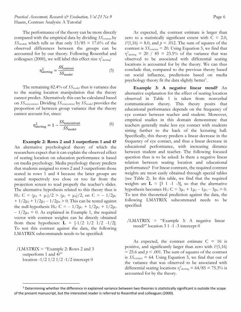
As expected, the contrast estimate is larger than zero to a statistically significant extent with C = 2.0, F(1,16) = 8.0, and p = .012. The sum of squares of the contrast is SScontrast = 20. Using Equation 5, we find that η2

alerting = 20 / 85 = 23.5% of the variance that was observed to be associated with differential seating locations is accounted for by the theory. We can thus conclude that, compared to the previous theory based on social influence, predictions based on media psychology theory fit the data slightly better3.

Example 3: A negative linear trend? An alternative explanation for the effect of seating location observed in Table 1 is taken from nonverbal communication theory. This theory posits that educational performance depends on the frequency of eye contact between teacher and student. Moreover, empirical studies in this domain demonstrate that teachers generally make less eye contact with students sitting further to the back of the lecturing hall. Specifically, this theory predicts a linear decrease in the frequency of eye contact, and thus a linear decrease in educational performance, with increasing distance between student and teacher. The following focused question thus is to be asked: Is there a negative linear relation between seating location and educational performance? For linear contrasts, the required contrast weights are most easily obtained through special tables (see Table 2). In this table, we find that the required weights are L = [3 1 -1 -3], so that the alternative hypothesis becomes H1: C = 3μ1 + 1μ2 ‒ 1μ3 ‒ 3μ4 > 0. To test this theoretical prediction against the data, the following LMATRIX subcommand needs to be specified:

/LMATRIX = “Example 3: A negative linear trend?” location 3 1 -1 -3 intercept 0

As expected, the contrast estimate C = 16 is positive, and significantly larger than zero with F(1,16) = 25.6 and p < .001. The sum of squares of the contrast is SScontrast = 64. Using Equation 5, we find that out of the variance that was observed to be associated with differential seating locations η2

alerting = 64/85 = 75.3% is accounted for by the theory.

Practical Assessment, Research & Evaluation, Vol 23 No 9 Page 7 Haans, Contrast Analysis: A Tutorial

We can thus conclude that of all three theories, predictions based on nonverbal communication theory fit the data best. Of course, the effects of seating location on educational performance may not be explained satisfactorily by a single theory; as often, multiple theories may be needed to explain all causal factors. In the next section, we discuss cases in which multiple theories are used to predict the data in Table 1.

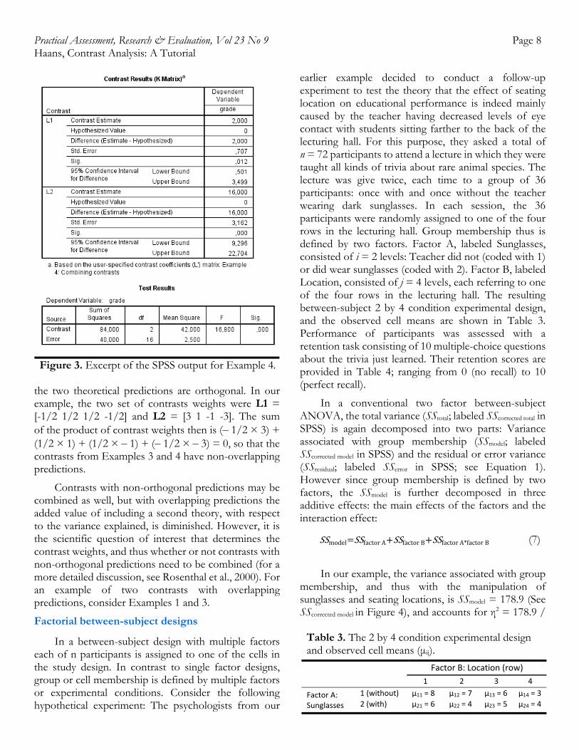
Example 4: Combining contrasts. The group of researchers in our example decided to test against the empirical data in Table 1 a prediction based on the two most promising theories: the nonverbal communication theory from Example 3, and the media psychology theory from Example 2. The first theory predicted a linear decrease in educational performance across the four rows because of a diminished frequency of eye contact over distance. The second theory predicted that students assigned two rows 2 and 3 would have better chances of performing well on the final exam, because they were seated at an appropriate distance from the projection screen: neither too close to (compared to row 1 students) nor too far from the screen (compared to row 4 students). Combined, the theories thus predict that the nonverbal benefit for row 1 students may be partly negated by them not being able to read the teacher’s slides properly. At the same time, the theories combined would predict a much lower performance of row 4 students, compared to their peers, then each theory would predict on its own. To test how well both theories combined predict the empirical effects of

seating location, the two contrasts need to be specified together in a single LMATRIX subcommand separated by a semicolon:

/LMATRIX = “Example 4: Combining contrasts” location -1/2 1/2 1/2 -1/2 intercept 0; location 3 1 -1 -3 intercept 0

SPSS will still provide the information in the Contrast Results table for each hypothesis separately, but the Test Results table will now provide the SScontrast and F-test for the combined prediction (see Figure 3). We find that F(2,16) = 16.8 with p < .001. Notice that the degrees of freedom of the nominator are two, and thus that the F-test is an omnibus test. We tested both contrasts against the empirical data simultaneously, but made no predictions about the relative importance of the two theories in predicting student grades. From this single F-test alone we, thus, cannot determine whether each individual contrast predicts a statistically significant part of the data, or what each prediction’s relative contribution is to the SScontrast.

The SScontrast of the combined prediction is 84. The prediction based on the two theories together thus predicts η2 = 84 / 125 = 67.2% of the overall variance in educational performance (using Equation 4); nearly as much as the variance observed to be associated with differential seating locations as determined with conventional ANOVA (i.e., 68%). This excellent performance of the combined prediction is more directly expressed with η2

alerting, which we calculate to be η2alerting =

84 / 85 = 98.8% (see Equation 5). In other words, the two theories combined explain nearly all of the observed between group variance—nearly all of the variance that is to be accounted for.

The attentive reader may notice that SScontrast in Figure 3 equals the sum of the sum of squares predicted by each theory separately (i.e., the sum of the SScontrast values for the contrasts in Examples 3 and 4). This is the case only when the combined contrasts are orthogonal or independent. Two theories have orthogonal predictions when differences between groups as predicted by one theory are not also (partly) predicted by the other. Whether two contrasts are orthogonal or not can be determined by taking the sum of the product of contrast weights for each cell (see Rosenthal et al., 2000). If the sum of products is ∑(lg,contrast1 × lg,contrast2) = 0, then

Table 2. Contrast weights for positive linear contrasts Contrast weights

Number of cells 1 2 3 4 5 6 7 8

2 -1 1

3 -1 0 1

4 -3 -1 1 3

5 -2 -1 0 1 2

6 -5 -3 -1 1 3 5

7 -3 -2 -1 0 1 2 3

8 -7 -5 -3 -1 1 3 5 7

Note. Table based on Rosenthal et al. (2000; p. 153). For an extended table including contrast weights for designs involving more groups or for quadratic contrasts see Rosenthal et al. (2000).

Practical Assessment, Research & Evaluation, Vol 23 No 9 Page 8 Haans, Contrast Analysis: A Tutorial

the two theoretical predictions are orthogonal. In our example, the two set of contrasts weights were L1 = [-1/2 1/2 1/2 -1/2] and L2 = [3 1 -1 -3]. The sum of the product of contrast weights then is (‒ 1/2 × 3) + (1/2 × 1) + (1/2 × ‒ 1) + (‒ 1/2 × ‒ 3) = 0, so that the contrasts from Examples 3 and 4 have non-overlapping predictions.

Contrasts with non-orthogonal predictions may be combined as well, but with overlapping predictions the added value of including a second theory, with respect to the variance explained, is diminished. However, it is the scientific question of interest that determines the contrast weights, and thus whether or not contrasts with non-orthogonal predictions need to be combined (for a more detailed discussion, see Rosenthal et al., 2000). For an example of two contrasts with overlapping predictions, consider Examples 1 and 3.

Factorial between-subject designs

In a between-subject design with multiple factors each of n participants is assigned to one of the cells in the study design. In contrast to single factor designs, group or cell membership is defined by multiple factors or experimental conditions. Consider the following hypothetical experiment: The psychologists from our

earlier example decided to conduct a follow-up experiment to test the theory that the effect of seating location on educational performance is indeed mainly caused by the teacher having decreased levels of eye contact with students sitting farther to the back of the lecturing hall. For this purpose, they asked a total of n = 72 participants to attend a lecture in which they were taught all kinds of trivia about rare animal species. The lecture was give twice, each time to a group of 36 participants: once with and once without the teacher wearing dark sunglasses. In each session, the 36 participants were randomly assigned to one of the four rows in the lecturing hall. Group membership thus is defined by two factors. Factor A, labeled Sunglasses, consisted of i = 2 levels: Teacher did not (coded with 1) or did wear sunglasses (coded with 2). Factor B, labeled Location, consisted of j = 4 levels, each referring to one of the four rows in the lecturing hall. The resulting between-subject 2 by 4 condition experimental design, and the observed cell means are shown in Table 3. Performance of participants was assessed with a retention task consisting of 10 multiple-choice questions about the trivia just learned. Their retention scores are provided in Table 4; ranging from 0 (no recall) to 10 (perfect recall).

In a conventional two factor between-subject ANOVA, the total variance (SStotal; labeled SScorrected total in SPSS) is again decomposed into two parts: Variance associated with group membership (SSmodel; labeled SScorrected model in SPSS) and the residual or error variance (SSresidual; labeled SSerror in SPSS; see Equation 1). However since group membership is defined by two factors, the SSmodel is further decomposed in three additive effects: the main effects of the factors and the interaction effect:

SSmodel SSfactorA SSfactorB SSfactorA*factorB (7)

In our example, the variance associated with group membership, and thus with the manipulation of sunglasses and seating locations, is SSmodel = 178.9 (See SScorrected model in Figure 4), and accounts for η2 = 178.9 /

Figure 3. Excerpt of the SPSS output for Example 4.

Table 3. The 2 by 4 condition experimental design and observed cell means (μij). 

Factor B: Location (row)

1  2  3  4 

Factor A: Sunglasses 

1 (without)  μ11 = 8  μ12 = 7  μ13 = 6  μ14 = 3 

2 (with)  μ21 = 6  μ22 = 4  μ23 = 5  μ24 = 4 

Practical Assessment, Research & Evaluation, Vol 23 No 9 Page 9 Haans, Contrast Analysis: A Tutorial

274.9 = 65.1% of the overall variance in retention scores (using Equation 2). With Sunglasses as Factor A and Location as Factor B, this variance is further decomposed in SSmodel = SSsunglasses + SSlocation

+ SSsunglasses*location (based on Equation 7). The SSsunglasses = 28.1 is the variance accounted for by the difference in retention when the teacher did or did not wear sunglasses, averaged across the levels of the Location factor (i.e., the variance accounted for by the main effect of Sunglasses). The null-hypothesis of the corresponding F-test is that there is such no main effect of wearing sunglasses. With F(1,64) = 18.8 and p < .001, this null-hypothesis is rejected.

The SSlocation = 111.4 is the variance accounted for by the average differences, aggregated across the two levels of the Sunglasses factor, in performance between students sitting in the various rows (i.e., the variance accounted for by the main effect of Location). The null-hypothesis of the corresponding F-test is that there is no such main effect of seating location. With F(3,64) = 24.8 and p < .001, this null-hypothesis can be rejected.

The SSsunglasses*location = 39.4 is the variance accounted for by the so-called difference of differences (e.g., Rosnow & Rosenthal, 1995): The effect of one factor

being different for the various levels of the other factor. The null-hypothesis of corresponding F-test is that no such differences of differences exist, and thus that the effect of Location is the same for both levels of the Sunglasses factor and vice versa. With F(3,64) = 8.8 and p < .001 this null-hypothesis can be rejected.

The researchers in our example, of course, did not conduct this experiment without a clear theoretical prediction in mind. If the nonverbal communication theory is correct, then the predicted decrease in performance across rows should not, or at least not as strongly, be observed when the teacher wore sunglasses. After all, by wearing dark sunglasses, the possibility of having eye contact is reduced equally for all students regardless of their seating location. The significant Sunglasses by Location interaction effect in Figure 4 may suggest that their theory is supported by the data—since their theory predicted the effects of Location to be different for the two levels of the sunglasses factor—, but the conventional ANOVA does not test the researchers’ prediction directly. As explained in the introduction, the interaction effect in a 2 by 4 design involves an omnibus test. As a result, there are multitudes of ways in which the effect of seating location may be different for the different levels of the sunglasses factor. Yet, only one of these possible differences of differences is predicted by the theory. In the next example, such specific predictions will be tested using contrast analysis.

When specifying the required set of contrast weights, one can generally ignore that group membership is defined by multiple factors. In other words, we can treat the example data as if they were obtained with an experiment that had a 1 by 8 design with g = 8 levels. This simplifies the required SPSS syntax, as L remains a row vector. As a result, the

Table 4. The data for the 2 by 4 condition experimental design.     Factor B: Location (row)

    1  2  3 4

Factor A: Sunglasses 

1 (without)  6  7  5 2

  7  9  8 2

  7  8  6 4

  8  8  7 3

  8  7  7 4

  8  6  4 3

  9  5  6 1

  9  6  5 3

  10  7  6 5

2 (with)  5  2  5 4

6  4  4 6

7  3  3 2

8  5  6 5

7  3  6 5

6  5  4 3

4  4  7 3

6  4  5 4

5  6  5 4

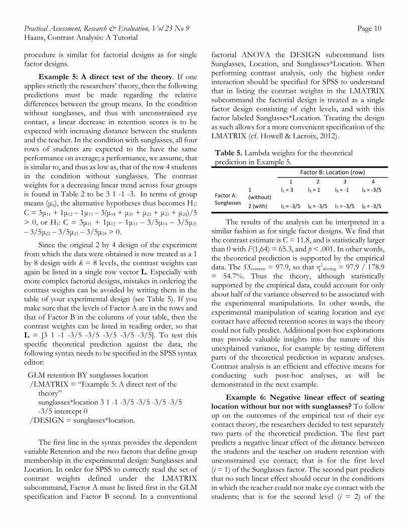
Table 5. Lambda weights for the theoretical prediction in Example 5. 

Factor B: Location (row)

1  2  3  4 

Factor A: Sunglasses 

1 (without) l1 = 3  l2 = 1  l3 = ‐1  l4 = ‐3/5

2 (with)  l5 = ‐3/5  l6 = ‐3/5  l7 = ‐3/5  l8 = ‐3/5

Figure 4. Excerpt of the SPSS output of a conventional between-subject ANOVA on the data of the 2 by 4 design in Table 4.

Practical Assessment, Research & Evaluation, Vol 23 No 9 Page 10 Haans, Contrast Analysis: A Tutorial procedure is similar for factorial designs as for single factor designs.

Example 5: A direct test of the theory. If one applies strictly the researchers’ theory, then the following predictions must be made regarding the relative differences between the group means. In the condition without sunglasses, and thus with unconstrained eye contact, a linear decrease in retention scores is to be expected with increasing distance between the students and the teacher. In the condition with sunglasses, all four rows of students are expected to the have the same performance on average; a performance, we assume, that is similar to, and thus as low as, that of the row 4 students in the condition without sunglasses. The contrast weights for a decreasing linear trend across four groups is found in Table 2 to be 3 1 -1 -3. In terms of group means (μij), the alternative hypotheses thus becomes H1: C = 3μ11 + 1μ12 ‒ 1μ13 ‒ 3(μ14 + μ21 + μ22 + μ23 + μ24)/5 > 0, or H1: C = 3μ11 + 1μ12 ‒ 1μ13 ‒ 3/5μ14 ‒ 3/5μ21 ‒ 3/5μ22 ‒ 3/5μ23 ‒ 3/5μ24 > 0.

Since the original 2 by 4 design of the experiment from which the data were obtained is now treated as a 1 by 8 design with k = 8 levels, the contrast weights can again be listed in a single row vector L. Especially with more complex factorial designs, mistakes in ordering the contrast weights can be avoided by writing them in the table of your experimental design (see Table 5). If you make sure that the levels of Factor A are in the rows and that of Factor B in the columns of your table, then the contrast weights can be listed in reading order, so that L = [3 1 -1 -3/5 -3/5 -3/5 -3/5 -3/5]. To test this specific theoretical prediction against the data, the following syntax needs to be specified in the SPSS syntax editor:

GLM retention BY sunglasses location /LMATRIX = “Example 5: A direct test of the theory” sunglasses*location 3 1 -1 -3/5 -3/5 -3/5 -3/5 -3/5 intercept 0 /DESIGN = sunglasses*location.

The first line in the syntax provides the dependent variable Retention and the two factors that define group membership in the experimental design: Sunglasses and Location. In order for SPSS to correctly read the set of contrast weights defined under the LMATRIX subcommand, Factor A must be listed first in the GLM specification and Factor B second. In a conventional

factorial ANOVA the DESIGN subcommand lists Sunglasses, Location, and Sunglasses*Location. When performing contrast analysis, only the highest order interaction should be specified for SPSS to understand that in listing the contrast weights in the LMATRIX subcommand the factorial design is treated as a single factor design consisting of eight levels, and with this factor labeled Sunglasses*Location. Treating the design as such allows for a more convenient specification of the LMATRIX (cf. Howell & Lacroix, 2012).

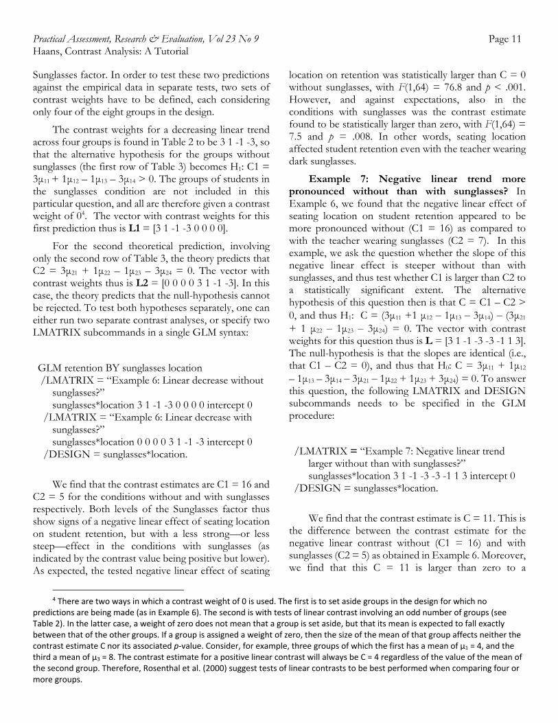
Table 5. Lambda weights for the theoretical prediction in Example 5.  Factor B: Location (row)

1  2  3  4 

Factor A: Sunglasses 

1 (without) 

l1 = 3  l2 = 1  l3 = ‐1  l4 = ‐3/5 

2 (with)  l5 = ‐3/5  l6 = ‐3/5  l7 = ‐3/5  l8 = ‐3/5 

The results of the analysis can be interpreted in a similar fashion as for single factor designs. We find that the contrast estimate is C = 11.8, and is statistically larger than 0 with F(1,64) = 65.3, and p < .001. In other words, the theoretical prediction is supported by the empirical data. The SScontrast = 97.9, so that η2

alerting = 97.9 / 178.9 = 54.7%. Thus the theory, although statistically supported by the empirical data, could account for only about half of the variance observed to be associated with the experimental manipulations. In other words, the experimental manipulation of seating location and eye contact have affected retention scores in ways the theory could not fully predict. Additional post-hoc explorations may provide valuable insights into the nature of this unexplained variance, for example by testing different parts of the theoretical prediction in separate analyses. Contrast analysis is an efficient and effective means for conducting such post-hoc analyses, as will be demonstrated in the next example.

Example 6: Negative linear effect of seating location without but not with sunglasses? To follow up on the outcomes of the empirical test of their eye contact theory, the researchers decided to test separately two parts of the theoretical prediction. The first part predicts a negative linear effect of the distance between the students and the teacher on student retention with unconstrained eye contact; that is for the first level (i = 1) of the Sunglasses factor. The second part predicts that no such linear effect should occur in the conditions in which the teacher could not make eye contact with the students; that is for the second level (i = 2) of the

Practical Assessment, Research & Evaluation, Vol 23 No 9 Page 11 Haans, Contrast Analysis: A Tutorial Sunglasses factor. In order to test these two predictions against the empirical data in separate tests, two sets of contrast weights have to be defined, each considering only four of the eight groups in the design.

The contrast weights for a decreasing linear trend across four groups is found in Table 2 to be 3 1 -1 -3, so that the alternative hypothesis for the groups without sunglasses (the first row of Table 3) becomes H1: C1 = 3μ11 + 1μ12 – 1μ13 – 3μ14 > 0. The groups of students in the sunglasses condition are not included in this particular question, and all are therefore given a contrast weight of 04. The vector with contrast weights for this first prediction thus is L1 = [3 1 -1 -3 0 0 0 0].

For the second theoretical prediction, involving only the second row of Table 3, the theory predicts that C2 = 3μ21 + 1μ22 – 1μ23 – 3μ24 = 0. The vector with contrast weights thus is L2 = [0 0 0 0 3 1 -1 -3]. In this case, the theory predicts that the null-hypothesis cannot be rejected. To test both hypotheses separately, one can either run two separate contrast analyses, or specify two LMATRIX subcommands in a single GLM syntax:

GLM retention BY sunglasses location /LMATRIX = “Example 6: Linear decrease without sunglasses?” sunglasses*location 3 1 -1 -3 0 0 0 0 intercept 0 /LMATRIX = “Example 6: Linear decrease with sunglasses?” sunglasses*location 0 0 0 0 3 1 -1 -3 intercept 0 /DESIGN = sunglasses*location.

We find that the contrast estimates are C1 = 16 and C2 = 5 for the conditions without and with sunglasses respectively. Both levels of the Sunglasses factor thus show signs of a negative linear effect of seating location on student retention, but with a less strong—or less steep—effect in the conditions with sunglasses (as indicated by the contrast value being positive but lower). As expected, the tested negative linear effect of seating

4 There are two ways in which a contrast weight of 0 is used. The first is to set aside groups in the design for which no 

predictions are being made (as in Example 6). The second is with tests of linear contrast involving an odd number of groups (see Table 2). In the latter case, a weight of zero does not mean that a group is set aside, but that its mean is expected to fall exactly between that of the other groups. If a group is assigned a weight of zero, then the size of the mean of that group affects neither the contrast estimate C nor its associated p‐value. Consider, for example, three groups of which the first has a mean of μ1 = 4, and the third a mean of μ3 = 8. The contrast estimate for a positive linear contrast will always be C = 4 regardless of the value of the mean of the second group. Therefore, Rosenthal et al. (2000) suggest tests of linear contrasts to be best performed when comparing four or more groups. 

location on retention was statistically larger than C = 0 without sunglasses, with F(1,64) = 76.8 and p < .001. However, and against expectations, also in the conditions with sunglasses was the contrast estimate found to be statistically larger than zero, with F(1,64) = 7.5 and p = .008. In other words, seating location affected student retention even with the teacher wearing dark sunglasses.

Example 7: Negative linear trend more pronounced without than with sunglasses? In Example 6, we found that the negative linear effect of seating location on student retention appeared to be more pronounced without (C1 = 16) as compared to with the teacher wearing sunglasses (C2 = 7). In this example, we ask the question whether the slope of this negative linear effect is steeper without than with sunglasses, and thus test whether C1 is larger than C2 to a statistically significant extent. The alternative hypothesis of this question then is that C = C1 – C2 > 0, and thus H1: C = (3μ11 +1 μ12 ‒ 1μ13 ‒ 3μ14) ‒ (3μ21 + 1 μ22 ‒ 1μ23 ‒ 3μ24) = 0. The vector with contrast weights for this question thus is L = [3 1 -1 -3 -3 -1 1 3]. The null-hypothesis is that the slopes are identical (i.e., that C1 – C2 = 0), and thus that H0: C = 3μ11 + 1μ12 – 1μ13 – 3μ14 ‒ 3μ21 ‒ 1μ22 + 1μ23 + 3μ24) = 0. To answer this question, the following LMATRIX and DESIGN subcommands needs to be specified in the GLM procedure:

/LMATRIX = “Example 7: Negative linear trend larger without than with sunglasses?” sunglasses*location 3 1 -1 -3 -3 -1 1 3 intercept 0 /DESIGN = sunglasses*location.

We find that the contrast estimate is C = 11. This is the difference between the contrast estimate for the negative linear contrast without (C1 = 16) and with sunglasses (C2 = 5) as obtained in Example 6. Moreover, we find that this C = 11 is larger than zero to a

Practical Assessment, Research & Evaluation, Vol 23 No 9 Page 12 Haans, Contrast Analysis: A Tutorial statistically significant extent, with F(1,64) = 18.2 and p < .001. This demonstrates that while constraining eye contact by wearing dark sunglasses may not completely remove the predicted linear effect of seating location on student retention, it does attenuate it to a statistically significant extent.

Contrast analysis in within-subject designs

Single factor within-subject designs

In a within-subject (or repeated measures) design each of n participants is assigned to all cells of the experimental design. Assume that the data in Table 1 were obtained with a repeated measures experiment, and that each row in Table 1 contains the data for a single participant. The single within-subject factor is labeled Location and consists of g = 4 levels. The sample then consists of n = 5 students, each of whom tested four times on their retention of the course materials: Once while sitting the first row (variable named row1), once sitting in the second row (row2), once sitting in third row (row3), and once sitting in the fourth and last row of the lecturing hall (row4). A conventional repeated-measure ANOVA on the data in Table 1 will tell the researchers what amount of variance in the data can be attributed to differences in seating location. The outcome of this test is reported in Figure 5.

In a within-subject ANOVA that involves a single factor, the overall variance in the data is decomposed into:

SStotal SSfactor SSperson SSfactor*person (8)

SSfactor is the variance associated with the effect of group membership, and thus the effect of the experimental manipulations. Since group membership is defined by a single factor SSfactor = SSmodel. Because we have repeated observations from each participant in within-subject designs, the residual term from the between-subject analysis (see Equation 1) can be decomposed into SSperson and SSfactor*person. The SSperson (labeled SSerror in SPSS) reflects overall individual differences in performance when aggregated across the four measurements (i.e., a main effect of person). The SSfactor*person (labeled SSerror(factor) in SPSS) is variance due to the experimental manipulations affecting different students differently (i.e., a person by factor interaction).

The SSfactor*person is the error term used in the calculation of the F-test for the effect of the within-subject factor.

In our example, the variance associated with group membership, and thus with the manipulation of seating locations is SSmodel = SSlocation = 85 (see the Tests of Within-Subjects Effects table in Figure 5). Its associated error term is SSlocation*person = 33.5. The effect of seating location is statistically significant with F(3,12) = 10.1 and p = .001. SPSS does not list SStotal in the output (see Figure 5), but the overall variance in the data can be calculated using Equation 8: SStotal = 85 + 6.5 + 33.5 = 125. We thus find that the effect of seating location can explain η2 = 85/125 = 68.0% of the overall variance in retention scores (using Equation 2).

Performing contrast analysis is rather similar for within- as for between-subject designs. In case of within-subject designs, each theoretical prediction is descripted by a row vector M (so-called transformation matrix) consisting of a series of contrast weights (mg), one for each of the g cells of the design (i.e., one for each repeated observation). The required contrast weights can be obtained in the same manner as before, but since the contrast weights now reflect expected differences between repeated observations, they have to be specified in an MMATRIX rather than an LMATRIX subcommand in the SPSS syntax.

There are small differences in how the MMATRIX subcommand is used compared to the LMATRIX subcommand. First, when an MMATRIX is specified the SScontrast cannot be compared directly to the SSmodel as obtained with a conventional within-subject ANOVA. As a result, the calculation of η2

alerting is slightly more complicated. Second, the MMATRIX subcommand can

Figure 5. Excerpt of the SPSS output of a conventional within-subject ANOVA on the data of the 1 by 4 design in Table 1

Practical Assessment, Research & Evaluation, Vol 23 No 9 Page 13 Haans, Contrast Analysis: A Tutorial only be included in the GLM syntax once. To test multiple predictions separately in one run (as in Example 6) the vectors with contrast weights have to be specified in a single MMATRIX subcommand. Finally, the way in which the contrast weights are listed in the syntax is slightly different for the MMATRIX subcommand. These differences will be explained in more detail in subsequent examples

Example 8: A negative linear trend? Let us test against the data of Table 1, now treated as originating from a within-subject design, the prediction based on nonverbal communication theory (see Example 3). This theory predicts a linear decrease in educational performance with increasing distance between student and teacher. The vector with contrast weights can again be obtained from Table 2: M = [3 1 -1 -3]. To test this prediction against the empirical data, the following syntax needs to be specified in SPSS syntax editor:

GLM row1 row2 row3 row4 /WSFACTOR=location 4 /MMATRIX="Example 8: A negative linear trend?" row1 3 row2 1 row3 -1 row4 -3 /MEASURE=grade /WSDESIGN=location.

The first line of the syntax provides the variable names of the repeated observations to be included in the General Linear Model (GLM) procedure (the variables labeled row1 to row4 in the dataset; see the online supplementary material). The WSFACTOR subcommand provides the name of the within-subject factor Location and its number of levels (g = 4). The WSDESIGN subcommand is used to specify the structure of the within-subject experimental design which in this example involves a single factor labeled Location. The optional MEASURE subcommand is used to provide a label for what was measured in each of the repeated observations (i.e., exam grades). Finally, the MMATRIX subcommand lists the contrast weights for each cell in the design (i.e., for each repeated observation). A more convenient alternative that does not require listing the name of each repeated variable in the MMATRIX subcommand is to use the ALL statement:

/MMATRIX = "Example 11: A negative linear trend?" ALL -3 -1 1 3

As before, you can either write the syntax directly in the syntax editor, or use the SPSS graphical user interface to set up a conventional repeated measures ANOVA, paste the instructions to the syntax editor, and add the MMATRIX subcommand manually. After running the syntax, the output of the analysis can be found in the SPSS output under the heading Custom Hypothesis Tests (see Figure 6).

The contrast estimate C = 16 is positive, and is statistically different from zero with F(1,4) = 44.9 and p = .003 (see Figure 6). In other words, we reject the null hypothesis which states that C = 0. The variance that can be explained by our theoretical prediction is SScontrast = 1280. When the prediction involves differences between repeated measures—i.e., when an MMATRIX subcommand is specified—this value cannot be directly compared with the outcome of the conventional repeated measures ANOVA reported in Figure 5. To do so, SScontrast first has to be divided by the sum of squared within-subject contrast weights (mg):

contrast

∑mg (9)

We find SS’contrast = 1280 / (32 + 12 + -12 + -32) = 1280 / 20 = 64. Based on Equation 5, we can calculate that η2

alerting = SS’contrast / SSlocation = 64 / 85 = 75.3%.

Figure 6. Excerpt of the SPSS output for Example 8.

Practical Assessment, Research & Evaluation, Vol 23 No 9 Page 14 Haans, Contrast Analysis: A Tutorial Factorial within-subject designs

In a factorial within-subject design, group membership is defined by two or more within-subject factors, and each of n participants is member of all groups. Assume that the data in Table 4 originated from a within-subject experiment in which group membership was defined by a Factor A labeled Sunglasses (consisting of i = 2 levels) and a Factor B labeled Location, (consisting of j = 4 levels, each referring to one of the

four rows in the lecturing hall). Treated as a within-subject experiment, each of n = 9 student were tested eight times on their retention of the course materials (with the data of the first person in the first and fifth row of Table 4, the data of the second person in the second and sixth row, and so forth). As with a between-subject factorial design (see Equation 7), a conventional within-subject ANOVA will explain the differences between groups in terms of two main effects and a Sunglasses by Location interaction effect. In repeated measures

Figure 7. Excerpt of the SPSS output of a conventional within-subject ANOVA on the data of the 2 by 4 design in Table 4.

Practical Assessment, Research & Evaluation, Vol 23 No 9 Page 15 Haans, Contrast Analysis: A Tutorial designs, however, each effect has its own specific error term. The SStotal is decomposed into:

SStotal SSfactorA SSfactorB SSfactorA*factorB SSperson SSfactorA*personSSfactorB*person SSfactorA*factorB*person

(10)

The SSfactorA*person (labeled SSerror(factorA) in SPSS), SSfactorB*person (labeled SSerror(factorB) in SPSS), and SSfactorA*factorB*person (labeled SSerror(factorA*factorB) in SPSS) are the error terms used in the calculation of the F-statistics for the main and interaction effects respectively. In our example, we find that SSsunglasses = 28.1, SSlocation = 111.4, and SSsunglasses*location = 39.4, so that, following Equation 7, SSmodel = 28.1 + 111.4 + 39.4 = 178.9 (see Figure 7). The SStotal can be calculated using Equation 10 and is SStotal = 28.1 + 111.4 + 39.4 + 23.8+ 6.8 + 21.3 + 44.3 = 275.2. Group membership, and thus the manipulation of sunglasses and seating location, then explains η2 = 178.9 / 275.2 = 65.0% of the overall variance in retention scores (using Equation 2).

Example 9: A direct test of the theory. To illustrate the use of the MMATRIX subcommand in factorial designs, let us consider the theoretical prediction of Example 5, but now with the data in Table 4 as resulting from a repeated-measures experiment with both Location and Sunglasses as within-subject factors. The required contrast weights (mg) are listed in Table 2: M = [3 1 -1 -3/5 -3/5 -3/5 -3/5 -3/5]. To test this theoretical prediction against the empirical data, the following syntax needs to be specified in the SPSS syntax editor. Note that in contrast to between-subject factorial designs (see Example 5), no modifications are needed to the WSDESIGN subcommand in order for SPSS to treat the 2 by 4 design as a 1 by 8:

GLM noglasses_row1 noglasses_row2 noglasses_row3 noglasses_row4 glasses_row1 glasses_row2 glasses_row3 glasses_row4 /WSFACTOR=sunglasses 2 location 4 /MMATRIX= "Example 9: A direct test of the theory?" ALL 3 1 -1 -3/5 -3/5 -3/5 -3/5 -3/5 /MEASURE=retention /WSDESIGN=sunglasses location sunglasses*location.

We find that the contrast estimate is C = 11.8 and is statistically different from 0 with F(1,8) = 143.9 and p < .001. In other words, the theoretical prediction is supported by the empirical data. The SScontrast = 1253.2. To calculate η2

alerting, we again first need to divide SScontrast by the sum of squared within-subject contrast weights (mg; see Equation 9): SS’contrast = 1253.2 / 12.8 = 97.9. Next we calculate η2

alerting using Equation 5: η2alerting = 97.9

/ 178.9 = 54.7%.

Example 10: Negative linear effect of seating location without but not with sunglasses? To illustrate the use of the MMATRIX subcommand for testing multiple contrasts in a single run of the GLM command, let us consider the two predictions tested in Example 6. The first prediction is a negative linear effect of seating location on student retention for the first level (i = 1) of the Sunglasses factor (i.e., when the teacher did not wear sunglasses). The second prediction is that no such linear effect should occur for the second level (i = 2) of the sunglasses factor (i.e., when the teacher was wearing sunglasses). The two vectors with the contrasts weights needed to test these two predictions are similar to those used in the between-subjects case in Example 6: M1 = [3 1 -1 -3 0 0 0 0] and M2 = [0 0 0 0 3 1 -1 -3], respectively.

In contrast to the LMATRIX subcommand, the MMATRIX subcommand can only be specified once in the GLM syntax. However, two sets of contrast weights can be included under the same MMATRIX subcommand separated by a semi-colon. In that case, SPSS will provide a univariate F-tests for each contrast separately, and a multivariate F-test for the combined prediction. To do so, the following MMATRIX subcommand needs to be specified in the GLM procedure:

/MMATRIX= "Example 10: Linear decrease without sunglasses?" ALL 3 1 -1 -3 0 0 0 0; "Example 10: Linear decrease with sunglasses?" ALL 0 0 0 0 3 1 -1 -3

The contrast estimate of each separate prediction is reported in the Contrast Results (K Matrix) table (see Figure 8). The F-test for each contrast is reported in the Univariate Test Results Table. We find that the contrast estimates are C1 = 16 and C2 = 5 for the conditions without and with sunglasses respectively. Both levels of

Practical Assessment, Research & Evaluation, Vol 23 No 9 Page 16 Haans, Contrast Analysis: A Tutorial

the Sunglasses factor thus show signs of a negative linear effect of seating location on student retention, but with a less strong—or less steep—effect in the conditions with sunglasses (as indicated by the contrast value being positive but lower). As expected, the tested negative linear effect of seating location on retention was statistically larger than C = 0 without sunglasses, with F(1,8) = 177.2, and p < .001. However, and against expectations, also in the conditions with sunglasses was the contrast estimate found to be statistically larger than zero, with F(1,8) = 8.4, and p = .020. In other words, seating location affected student retention even with the teacher wearing dark sunglasses. The test of the combined prediction is provided in the Multivariate Test Results table in Figure 8, but as a multivariate rather than a univariate ANOVA test.

When comparing the η2alerting of the two predictions,

it becomes clear that the linear decrease in retention over distance is much more prevalent without than with the teacher wearing sunglasses. In the condition without sunglasses the negative linear trend explained η2

alerting = 64.4% of the variance empirically associated with the manipulation of sunglasses and seating location. In contrast, only η2

alerting = 6.3% of this variance is explained in the condition with sunglasses. To calculate these

effect sizes we first have to divide the SScontrast by the sum of squared within-subject contrast weights in M (see Equation 9). For the condition without sunglasses, we find that SScontrast = 2304 (see the Univariate Test Results table in Figure 8). Divided by the sum of squared contrast weights (mg), we find that SS’contrast = 2304 / 20 = 115.2 (using Equation 9). Next we use Equation 5 to calculate that η2

alerting = SS’contrast / SSmodel = 115.2 / 178.9 = 64.4%. For the condition with sunglasses, we find that SScontrast = 225, so that SS’contrast = 225 / 20 = 11.3, and that η2

alerting = 11.3 / 178.9 = 6.3%.

Mixed designs

In mixed designs, group membership is defined by a combination of between- and within-subject factors. As a result, each of n participants is member of some but not all of the cells in the design. Assume that the data in Table 4 originated from a mixed design experiment in which group membership was defined by a between-subject Factor A labeled Sunglasses (consisting of i = 2 levels) and a within-subject Factor B labeled Location, (consisting of j = 4 levels, each referring to one of the four rows in the lecturing hall). In this case, each of n = 18 students were tested 4 times on their retention of the course materials (i.e., while sitting first, second, third, or fourth row from the teacher) but with the teacher either wearing or not wearing sunglasses. As a result each row in Table 4 contains the retention scores from a single participant.

With this mixed design, the variance in the data, or SStotal, is decomposed into:

SStotal SSfactorA SSfactorB SSperson|factorASSfactorA*factorB SSfactorB*person|factorA

(13)

The SSperson|factorA (labeled SSerror in SPSS) is the error term used in the calculation of the F-statistic for the main effect of the between subject factor (in this case Sunglasses). The SSfactorB*person|factorA (labeled SSerror(factorB) in SPSS), in turn, is used as the error term for the main effect of the within-subject factor (in this case Location), and for the interaction between the within- and between- subject factor (in this case the Location*Sunglasses interaction). In our example, we find that SSsunglasses = 28.1, SSlocation = 111.4, and SSlocation*sunglasses = 39.4 (see Figure 9), so that, based on Equation 7, SSmodel = 178.9. The SStotal can be calculated using Equation 13 and is

Figure 8: Excerpt of the SPSS output for Example 10.

Practical Assessment, Research & Evaluation, Vol 23 No 9 Page 17 Haans, Contrast Analysis: A Tutorial

SStotal = 111.4 + 28.1 + 30.5 + 39.4 + 65.5 = 274.9. Group membership, and thus the manipulation of sunglasses and seating location, is found to be associated to η2 = 178.9 / 274.9 = 65.1% of the overall variance in retention scores (using Equation 2).

In the case of mixed designs, each theoretical prediction is described by a matrix W consisting of a series of contrast weights (wij), one for each cell in the design. What complicates contrast analysis on mixed designs is that the factorial structure of the experimental design cannot be ignored: The 2 (Sunglasses) by 4 (Location) design cannot be treated as a 1 by 8 design. As a result the set of contrast weights (W) is a matrix rather than a vector. For example, the theoretical prediction that the negative linear effect of seating location on student retention is more pronounced without than with sunglasses (as tested in Example 10 for a between-subject design) becomes W = [3 1 -1 -3; -3 -1 1 3]. To test such a prediction against the empirical

data, matrix W has to be decomposed into two vectors—one for the between-subject part (which we labeled L), the other for the within-subject part of the design (which we labeled M)—that when multiplied yield the desired matrix W, where W = LT × M. The vector L has to be specified in the LMATRIX, and the vector M in the MMATRIX subcommand. The examples below explain how these two vectors can be obtained.

Consequently, there are limits to the theoretical predictions one can test with mixed designs. For example, the theoretical prediction of Example 5 cannot be tested when the data in Table 4 result from an experiment with a combination of between- and within-subject factors: There is no combination of L and M vectors whose multiplication will yield LT × M = W = [3 1 -1 -3/5; -3/5 -3/5 -3/5 -3/5]. Interpreting the outcomes of a contrast analysis is, however, similar for mixed as for between- and within-subject designs.

Figure 9: Excerpt of the SPSS output of a conventional mixed ANOVA on the data of the 2 by 4 design in Table 4 with Sunglasses as between- and Location as within-subject factor.

Practical Assessment, Research & Evaluation, Vol 23 No 9 Page 18 Haans, Contrast Analysis: A Tutorial

Example 11: Negative linear effect of seating location without but not with sunglasses? Let us once more test the two predictions from Examples 6 and 10, but this time while treating the Sunglasses as a between-subject and Location as a within-subject factor. The first prediction is a negative linear effect of seating location on student retention for participants assigned to the first level (i = 1) of the Sunglasses factor (i.e., when the teacher did not wear sunglasses). The matrix of contrast weights that define this expectation, as determined in Example 6, is W1 = [3 1 -1 -3; 0 0 0 0]. The second prediction involves a similar negative linear effect of seating location but for the condition with sunglasses: W2 = [0 0 0 0; 3 1 -1 -3].

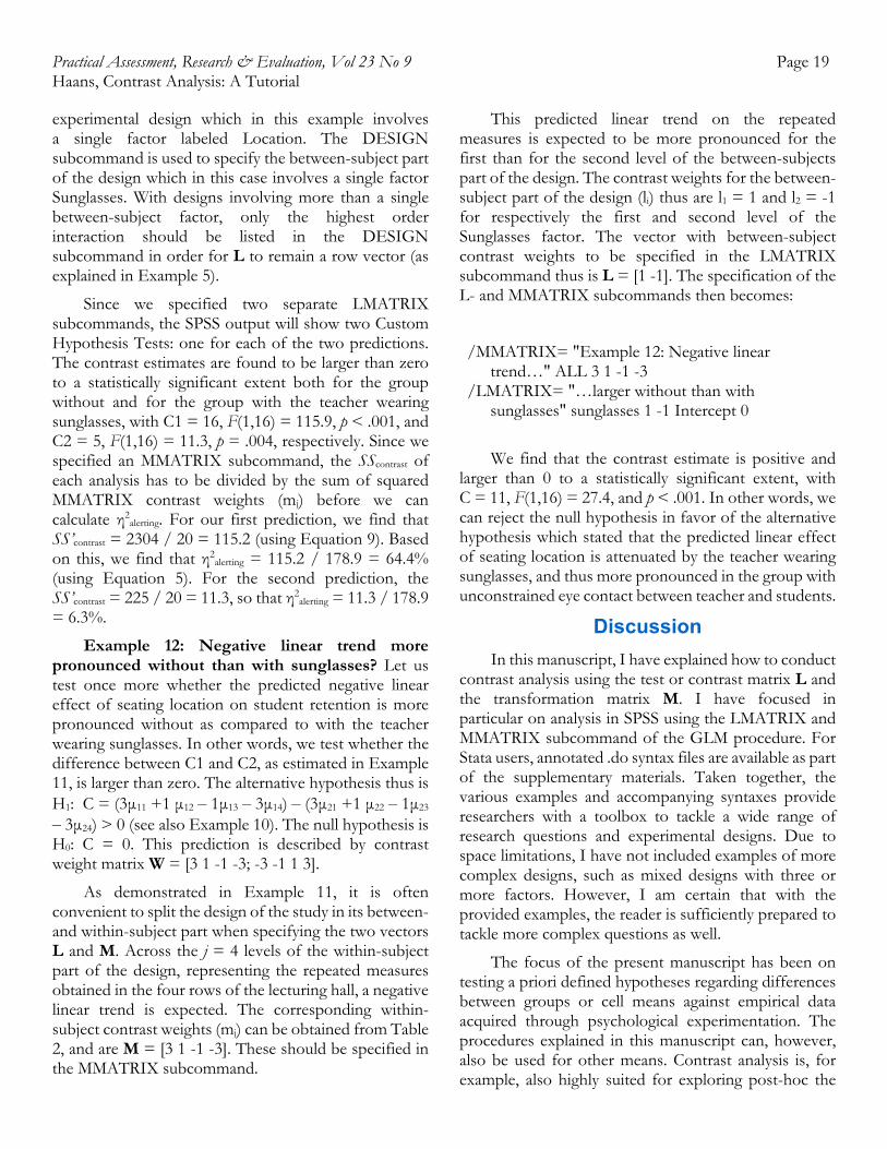
To determine the vectors L and M for these two predictions, and thus to determine what contrast weights have to be specified in the LMATRIX and MMATRIX subcommands, it is often convenient to split the design in Table 3 into its between- and within-subject part (see Table 6). In this relatively simple two-factor design, the between-subject part comprises the Sunglasses factor, and the within-subject part the Location factor.

The theoretical prediction specified by W1 is a negative linear effect of seating location on retention scores for students whose teacher did not wear sunglasses. In the within-subject part of the design in Table 6, we can list the contrast weights (mj) that correspond to such a negative linear effect of seating location. These contrast weights can be obtained from Table 2: 3 1 -1 -3. These four weights form vector M = [3, 1, -1, -3] and have to be listed in the MMATRIX subcommand of the GLM procedure.

The first prediction pertains only to the participants whose teacher did not wear sunglasses, and we can thus set aside the second level of the Sunglasses factor by assigning its contrast weight a value of l2 = 0 in the between-subject part of the design in Table 6. Finally, we assign the first level of the Sunglasses factor a contrast weight of l1 = 1 in the between-subject part of the Table 6, so that the linear effect specified by M is tested only for the group in the no sunglasses condition. These two

weights form vector L1 = [1 0] and have to be listed in the LMATRIX subcommand in the GLM syntax. The specification of the LMATRIX and MMATRIX subcommands for the first prediction thus becomes:

/MMATRIX= "Example 11: negative linear trend…" ALL 3 1 -1 -3 /LMATRIX= "…without sunglasses?" sunglasses 1 0 intercept 1

Note that the weight of the intercept (l0) in the LMATRIX subcommand is 1. As explained in Example 1, the weight of the intercept can be calculated by taking the sum of the contrast weights (li) specified in the LMATRIX subcommand: l0 = ∑li.

To test the second prediction against the empirical data, we can add an additional LMATRIX subcommand in which the contrast weights (li) are reversed, so that L2 = [0 1]. This way, the linear prediction specified under the MMATRIX subcommand will be tested on the group of which the teacher wore sunglasses. The full syntax then becomes:

GLM row1 row2 row3 row4 BY sunglasses /WSFACTOR=location 4 /MMATRIX= "Example 11: Negative linear trend…" ALL 3 1 -1 -3 /LMATRIX= "…without sunglasses?" sunglasses 1 0 intercept 1 /LMATRIX= "…with sunglasses?" sunglasses 0 1 intercept 1 /MEASURE=retention /WSDESIGN=location /DESIGN=sunglasses.

The first line of the syntax provides the variable names of the repeated observations to be included in the General Linear Model (GLM) procedure (the variables labeled row1 to row4 in the dataset; see supplementary materials). The WSFACTOR subcommand provides the name of the within-subject factor Location and its number of levels (g = 4). The optional MEASURE subcommand is used to provide a label for what was measured in each of the repeated observations (i.e., exam grades). The WSDESIGN subcommand is used to specify the structure of the within-subject part of

Table 6. L and M contrast weights for prediction W1 in Example 11. 

Between‐subject part: Sunglasses

Within subject part: Location (row)

1  2  3  4 

  L  m1 = 3  m2 = 1  m3 = ‐1  m4 = ‐3  M

1 (without)  l1 = 1  w11 = 3  w12 = 1  w13 = ‐1  w14 = ‐3   2 (with)  l2 = 0  w21 = 0  w22 = 0  w23 = 0  w24 = 0   

Practical Assessment, Research & Evaluation, Vol 23 No 9 Page 19 Haans, Contrast Analysis: A Tutorial experimental design which in this example involves a single factor labeled Location. The DESIGN subcommand is used to specify the between-subject part of the design which in this case involves a single factor Sunglasses. With designs involving more than a single between-subject factor, only the highest order interaction should be listed in the DESIGN subcommand in order for L to remain a row vector (as explained in Example 5).

Since we specified two separate LMATRIX subcommands, the SPSS output will show two Custom Hypothesis Tests: one for each of the two predictions. The contrast estimates are found to be larger than zero to a statistically significant extent both for the group without and for the group with the teacher wearing sunglasses, with C1 = 16, F(1,16) = 115.9, p < .001, and C2 = 5, F(1,16) = 11.3, p = .004, respectively. Since we specified an MMATRIX subcommand, the SScontrast of each analysis has to be divided by the sum of squared MMATRIX contrast weights (mj) before we can calculate η2

alerting. For our first prediction, we find that SS’contrast = 2304 / 20 = 115.2 (using Equation 9). Based on this, we find that η2

alerting = 115.2 / 178.9 = 64.4% (using Equation 5). For the second prediction, the SS’contrast = 225 / 20 = 11.3, so that η2

alerting = 11.3 / 178.9 = 6.3%.

Example 12: Negative linear trend more pronounced without than with sunglasses? Let us test once more whether the predicted negative linear effect of seating location on student retention is more pronounced without as compared to with the teacher wearing sunglasses. In other words, we test whether the difference between C1 and C2, as estimated in Example 11, is larger than zero. The alternative hypothesis thus is H1: C = (3μ11 +1 μ12 ‒ 1μ13 ‒ 3μ14) ‒ (3μ21 +1 μ22 ‒ 1μ23 ‒ 3μ24) > 0 (see also Example 10). The null hypothesis is H0: C = 0. This prediction is described by contrast weight matrix W = [3 1 -1 -3; -3 -1 1 3].

As demonstrated in Example 11, it is often convenient to split the design of the study in its between- and within-subject part when specifying the two vectors L and M. Across the j = 4 levels of the within-subject part of the design, representing the repeated measures obtained in the four rows of the lecturing hall, a negative linear trend is expected. The corresponding within-subject contrast weights (mj) can be obtained from Table 2, and are M = [3 1 -1 -3]. These should be specified in the MMATRIX subcommand.

This predicted linear trend on the repeated measures is expected to be more pronounced for the first than for the second level of the between-subjects part of the design. The contrast weights for the between-subject part of the design (li) thus are l1 = 1 and l2 = -1 for respectively the first and second level of the Sunglasses factor. The vector with between-subject contrast weights to be specified in the LMATRIX subcommand thus is L = [1 -1]. The specification of the L- and MMATRIX subcommands then becomes:

/MMATRIX= "Example 12: Negative linear trend…" ALL 3 1 -1 -3 /LMATRIX= "…larger without than with sunglasses" sunglasses 1 -1 Intercept 0

We find that the contrast estimate is positive and larger than 0 to a statistically significant extent, with C = 11, F(1,16) = 27.4, and p < .001. In other words, we can reject the null hypothesis in favor of the alternative hypothesis which stated that the predicted linear effect of seating location is attenuated by the teacher wearing sunglasses, and thus more pronounced in the group with unconstrained eye contact between teacher and students.

Discussion

In this manuscript, I have explained how to conduct contrast analysis using the test or contrast matrix L and the transformation matrix M. I have focused in particular on analysis in SPSS using the LMATRIX and MMATRIX subcommand of the GLM procedure. For Stata users, annotated .do syntax files are available as part of the supplementary materials. Taken together, the various examples and accompanying syntaxes provide researchers with a toolbox to tackle a wide range of research questions and experimental designs. Due to space limitations, I have not included examples of more complex designs, such as mixed designs with three or more factors. However, I am certain that with the provided examples, the reader is sufficiently prepared to tackle more complex questions as well.

The focus of the present manuscript has been on testing a priori defined hypotheses regarding differences between groups or cell means against empirical data acquired through psychological experimentation. The procedures explained in this manuscript can, however, also be used for other means. Contrast analysis is, for example, also highly suited for exploring post-hoc the

Practical Assessment, Research & Evaluation, Vol 23 No 9 Page 20 Haans, Contrast Analysis: A Tutorial often complex interactions obtained with conventional ANOVA. For more information on how to use contrast analysis to follow-up on significant omnibus interaction tests, and on how to deal with multiple comparisons (i.e., the inflation of experiment-wise Type I errors), the interested reader is referred to Abelson and Prentice (1997), Howell and Lacroix (2012), and Jaccard and Guilamo-Ramos (2002a; 2002b).

I also have not discussed the assumptions behind contrast analysis as these are similar to conventional ANOVA, including that the observations are normally distributed in each group or cell of the design, that population variances of each group are identical, and that observations are independent (see, e.g., Stevens, 2007). The often violated sphericity assumption that applies to within-subject factors typically does not apply to contrast analysis as violations of sphericity cannot occur with focused tests (i.e., with test that have a single degree of freedom). Only when the combined prediction of two contrasts are tested on a within-subject factor (as in Example 10) can violations of sphericity be problematic. In these cases, however, most statistical software packages perform a multivariate rather than a univariate test of significance for which sphericity is not required (see, e.g., Stevens, 2007).

Many textbooks dictate the use of factorial ANOVA in which differences between group or cell means are explained by a series of main and interaction effects, whether these answer the researcher’s questions of interest or not. As discussed in the onset of the manuscript, this curious convention—called factorial ANOVA—not only puts researchers at risk of committing what Hand (1994) called a type III error, but may also lead them to face undue difficulties in following up on statistically significant main and interaction effects through a combination of eye-balling graphs or conducting additional post-hoc analyses; analyses that are often as uninformative as the main and interaction effects themselves. Contrast analysis can save us from these burdens, and my hope is that the present manuscript can make a modest contribution to making the technique more accessible in its use.

References

Abelson, P. R., & Prentice, D. A. (1997). Contrast test for interaction hypothesis. Psychological Methods, 2(4), 315-328. doi: 10.1037/1082-989X.2.4.315

Cohen, J. (1990). Things I have learned (so far). American Psychologist, 45, 1304-1312. doi: 10.1037/0003-066X.45.12.1304

Haans, A. (2008). What does it mean to be average? The gallons per mile versus miles per gallon paradox revisited. Practical Assessment, Research & Evaluation, 13(3). Available online: http://pareonline.net/getvn.asp?v=13&n=3

Hand, D. J. (1994). Deconstructing statistical questions. Journal of the Royal Statistical Society A, 157, 317-356. doi: 10.2307/2983526

Howell, G. T., & Lacroix, G. L. (2012). Decomposing interactions using GLM in combination with the COMPARE, LMATRIX, and MMATRIX subcommands in SPSS. Tutorials in Quantitative Methods for Psychology, 8, 1-22. doi: 10.20982/tqmp.08.1.p001

IBM Corp. (2013). IBM SPSS Statistics 22 command syntax reference. Armonk, NY: IBM Corp.

Jaccard, J., & Guilamo-Ramos, V. (2002a). Analysis of variance frameworks in clinical child and adolescent psychology: Issues and recommendations. Journal of Clinical Child and Adolescent Psychology, 31(1), 130-146. doi: 10.1207/S15374424JCCP3101_15

Jaccard, J., & Guilamo-Ramos, V. (2002b). Analysis of variance frameworks in clinical child and adolescent psychology: Advanced issues and recommendations. Journal of Clinical Child and Adolescent Psychology, 31(2), 278-294. doi: 10.1207/S15374424JCCP3102_13

Rosenthal, R., Rosnow, R. L., & Rubin, D. R. (2000). Contrast and effect sizes in behavioral research: A correlational approach. Cambridge, UK: Cambridge University Press.

Rosnow, R. L., & Rosenthal, R. (1995). “Some things you learn aren’t so”: Cohen’s paradox, Asch’s paradigm, and the interpretation of interaction. Psychological Science, 6, 3-9. doi: 10.1111/j.1467-9280.1995.tb00297.x

Rosnow, R. L., & Rosenthal, R. (1996). Contrasts and interaction redux: Five easy pieces. Psychological Science, 7, 253-257. doi: 10.1111/j.1467-9280.1996.tb00369.x

Statacorp LP (2015). Stata multivariate statistics reference manual (Release 14). College Station, Texas: Stata press.

Stevens, J. P. (2007). Intermediate statistics: A modern approach. New York: Lawrence Erlbaum Associates.

Wiens, S., & Nilsson, M. E. (2017). Performing contrast analysis in factorial designs: From NHST to confidence intervals and beyond. Educational and Psychological Measurement, 77, 690-715. doi: 10.1177/0013164416668950

Practical Assessment, Research & Evaluation, Vol 23 No 9 Page 21 Haans, Contrast Analysis: A Tutorial

Note:

The results in this paper can be replicated using the data and syntax for Stata or SPSS found in http://pareonline.net/sup/v23n9.zip

Citation:

Haans, Antal (2018). Contrast Analysis: A Tutorial. Practical Assessment, Research & Evaluation, 23(9). Available online: http://pareonline.net/getvn.asp?v=23&n=9

Corresponding Author

Antal Haans Eindhoven University of Technology P.O. Box 513 NL-5600 MB Eindhoven The Netherlands email: a.haans [at] tue.nl