Contract, Mechanism Design,and Technological Detail

Joel Watson∗

Preliminary version, May 2001Revised January 2002

Abstract

This paper develops a theoretical framework for studying contract and en-forcement in settings of complete, but unverifiable, information. The mainpoint of the paper is that the consideration of renegotiation necessitates for-mal examination of other technological constraints, especially those having todo with the timing and nature of inalienable productive decisions. The maintechnical contributions include (a) results that characterize of the sets of imple-mentable state-contingent payoffs under various assumptions about renegotia-tion opportunities, and (b) a result establishing conditions under which, whentrading opportunities are durable and trade decisions are reversible, station-ary contracts are optimal. The analysis refutes the validity of the “mechanismdesign with ex post renegotiation” program, it demonstrates the validity ofother mechanism design models in dynamic environments, and it highlightsthe need for a more structured game-theoretic framework. JEL Classification:C70, D74, K10.

∗University of California, San Diego. Internet: http://weber.ucsd.edu/∼jwatson/. I thank JesseBull, Vince Crawford, Aaron Edlin, Oliver Hart, W. Bentley MacLeod, John Moore, Joel Sobel, andmy colleagues at UC San Diego for their comments. The research reported herein is supported byNSF grant SES-0095207.

1

Economic models of contract have yielded important insights regarding the na-ture of contractual imperfections, optimal contractual form, and contractual scope.Many of the insights derive from mechanism design analysis, which strips away insti-tutional details to focus on just a few fundamental ingredients. Mechanism design isan abstract and elegant methodology. The mathematical elegance comes at a cost,however, to the extent that real institutions and technology limit the formation andenforcement of contracts.Researchers have rightly turned their attention to the actual constraints that

institutions impose, in an attempt to clarify our understanding of contractual imper-fections and to inform the design of enforcement systems. One issue that has receiveda great deal of attention is the possibility that parties can renegotiate in the midst of acontractual relationship. Hart and Moore’s (1988) seminal article shows how renego-tiation following specific investments can greatly inhibit the parties’ ability to attainan efficient outcome. Recently, theorists have attempted to incorporate renegotiationconstraints into otherwise standard mechanism design analysis. Maskin and Moore(1999) developed the basic mechanism design with ex post renegotiation (MDER) pro-gram, which assumes that parties can renegotiate the contractually-specified outcomeafter sending messages to an external enforcer. Maskin and Moore’s methodology andcharacterization results have been widely accepted and employed.1

In this paper, I study how renegotiation opportunities interact with the productivetechnology of contractual relationships. Specifically, I do two things. First, I showthat, in order to adequately address renegotiation, we must account for the technol-ogy of trade. In other words, our models must explicitly describe the timing andnature of productive actions. Second, I develop a general analytical framework and Icharacterize the set of implementable outcomes under a variety of assumptions aboutwhen renegotiation can take place. My main technical result is that, for most envi-ronments in which trade decisions can be reversed, stationary contracts are optimaland implementability does not depend on the degree to which trading opportunitiesare durable.My results do not challenge the legitimacy of mechanism design theory for the

study of contract. However, my results reveal that the application of mechanismdesign theory can be seriously flawed if one does not incorporate the proper techno-logical constraints. Indeed, I show that a segment of the contract theory literaturehas such a flaw. Specifically, I find that the popular MDER program never accuratelydescribes the scope of contracting; this program can only be justified on the basis ofunreasonable incompleteness assumptions that are hidden in the current literature.

1The MDER program builds from Maskin’s (1999) seminal contribution on Nash implementation(without renegotiation). The literature contains numerous, high-profile papers that adopt the MDERprogram, including the important work of Che and Hausch (1999), Edlin and Reichelstein (1996),Segal (1999), and Segal and Whinston (2000).

2

On the other hand, I show that the “mechanism design with interim renegotiation”(MDIR) program, which assumes that renegotiation occurs only before parties sendmessages to an external enforcer, is justified in some settings.To see the main idea behind my research, consider the mechanism design ideal.

The mechanism design program starts with a set of players, a set of states (describingthe informational setting), a set of outcomes (describing those things players careabout that can be controlled publicly), and a specification of preferences over statesand outcomes. For a contractual setting, the outcome is usually assumed to describeverifiable trade decisions, which an external enforcement authority can compel. Thenthe scope of enforceable contracts is given by the set of mechanisms (game forms).The goal of contracting is to implement the players’ preferred state-contingent valuefunction, which either helps them share risk or gives them the incentive to makeinvestments that influence the state.Within this mechanism design framework, institutional constraints are best mod-

elled as a limit on the class of mechanisms. To represent the “ex post renegoti-ation” constraint, for example, theorists have focused on game forms with a finaloutcome-renegotiation stage, where the players always negotiate–with fixed bargain-ing weights–to an ex post efficient outcome, subject to some contractually-specifieddefault outcome. Ex post renegotiation is a convenient modeling component, be-cause the resulting constrained mechanism design problem can be easily transformedinto a standard unconstrained problem. To get the unconstrained representation,one simply redefines the players’ payoffs over outcomes to be the post-renegotiationpayoffs.2

The problem with abstract assumptions such as “ex post renegotiation” is that,because they have no direct institutional foundation, they are difficult to interpret.Questions such as “Does renegotiation occur before or after verifiable trade deci-sions?” and “How does an external enforcer compel a particular trade decision whenplayers can renegotiate ex post?” have no clear answers. To provide answers to thesequestions, and to understand the effect of renegotiation opportunities, one must sortout the timing of trade, enforcement, and renegotiation. This requires dispensingwith the treatment of verifiable trade decisions as “public.”My framework has a more detailed theoretical foundation than is common in the

literature. I develop a structured, game-theoretic model that explicitly accounts forthe following essential elements: (a) the timing and nature of individual, inalien-able decisions; (b) the manner in which the external enforcer compels behavior; and(c) at what times the parties have the opportunity to renegotiate their contract.3

2On a technical level, ex post renegotiation also creates useful theoretical regularities. Segal andWhinston’s (2000) differential analysis takes advantage of these.

3My approach is thus allied with that of Hart and Moore (1988), MacLeod and Malcomson(1993), and Noldeke and Schmidt (1995), who model individual trade decisions. I elaborate on this

3

With these elements in place, one can clearly describe and interpret renegotiationconstraints. Regarding (a), observe that, in reality, most trade decisions are inalien-able; for example, a buyer and a seller cannot instruct the court to deliver the goodthat they wish to exchange.4 Thus, on (b), courts do not enforce trading outcomesby actually making the trade decisions for the contracting parties. Rather, enforce-ment occurs via transfers and penalties that courts compel conditional on the parties’verifiable, individual trade decisions.5

The key observation–which is obvious once trade decisions are formally modelled–is that there are two ways of building options into contracts. First, a contract cantrigger externally enforced transfers on the basis of whether a party sends a partic-ular verifiable message before the trading opportunity. Second, the trade decisionsthemselves may serve as options, with the externally enforced transfer simply a func-tion of the parties’ behavior.6 There is no practical difference between using thesetwo types of options in the absence of renegotiation opportunities. However, whenrenegotiation is possible, its effect depends on whether it can occur (i) before theparties send messages or (ii) between the message phase and when the parties maketrade decisions. In the former case, renegotiation affects implementability exactly ascharacterized by the MDIR program. In the latter case, message-based options aresubject to renegotiation. Parties can avoid the detrimental consequences of renego-tiation by using trade decisions as options, but the technology of trade limits thescope of this scheme. Implementability in this case is not characterized by any of theliterature’s standard mechanism design programs.The following section contains the analysis of an extended example, in which the

contracting parties face a nondurable trading opportunity. The example introducesmy modeling framework and it illustrates my basic points. I examine three differentsettings that are distinguished by when, if ever, the contracting parties can renegotiatetheir contract. I characterize the set of implementable state-contingent payoff vectors

in the next section.4Or, at least, the court would not honor such a request. In a mechanism design model, inalienable

trade decisions imply a constraint on the class of mechanisms. For example, suppose that, in aparticular trading relationship, the seller must decide whether to deliver intermediate good A, goodB, or nothing. Then, the mechanism must be a game form in which the seller makes this decisionat some point. Because the decision is inalienable, we cannot have a mechanism that specifies only,say, the “good A” and “nothing” outcomes (so that the seller is not allowed to choose “good A”).

5Specific performance, for instance, is a court order to act (under penalty of contempt) ratherthan the court taking the action on behalf of the contracting party.

6Mechanism design models study options of the first type; more structured models, such asNoldeke and Schmidt’s (1995), focus on the second type. The law treats option generally, as a limiton a parties “power to revoke an offer” (Section 25, Restatement (Second) of Contracts; see Barnett1999). In addition to more conventional forms, options are implicitly created by liquidated damageprovisions and standard breach remedies. (A party has the option of breaching and then paying thedamage amount.)

4

for each setting and I relate them to the set identified by the standard mechanismdesign programs from the literature.Sections 2-5 define and analyze my general modeling framework. Section 2 de-

scribes a “period” of interaction, in which the contracting parties form and renegotiatetheir contract, make trade decisions, and interact with the external enforcer. In Sec-tion 3, I derive necessary conditions for the implementation of state-contingent payoffvectors under various assumptions about when the parties can renegotiate.In Section 4, I explain how to model settings in which the trading opportunities are

durable and trade decisions are reversible. In such settings, the parties interact overan infinite number of periods. The parties can make any particular trade decisionin one period and then reverse it in a future period. Parties can write long-termcontracts and they can renegotiate at various dates within a period.Section 5 contains my technical results. I provide a theorem that ranks by inclusion

the sets of implementable state-contingent payoffs under various assumptions aboutrenegotiation. This result formalizes for a very general environment what the exampleof Section 1 demonstrates. I then present the main result–that for most of thesettings studied here, stationary contracts are always optimal. This result impliesthat the parties’ long-term contracting problem can be reduced to a simple staticproblem, which has important positive and normative implications and clarifies theproper use of mechanism design theory. The optimality of stationary contracts furtherimplies that the extent of durability is irrelevant to the contracting problem, whichgives a useful benchmark for future theoretical work.Section 6 comprises two examples that further clarify the shortcomings of the

MDER program while confirming, with qualifications, that hold-up is indeed a prob-lem in some contractual relationships. Section 7 contains concluding remarks.Numerous authors have argued for the kind of research reported herein. Hurwicz

(1994) speaks of the importance of incorporating institutional constraints into de-sign problems–a step that, for the most part, has yet to be taken in any general,compelling way. He suggests that institutional constraints should be represented aslimiting design to a class of game forms, whereby the “ ‘desired’ game form [is em-bedded in what he calls] the ‘natural’ game form” (p.12). My framework may beinterpreted as this natural game form. Anderlini, Felli, and Postlewaite (2001), Segaland Whinston (2000), and others recognize the need to study technological and insti-tutional constraints in contracting environments. Furthermore, the contract theoryliterature has seen several debates regarding renegotiation and its relation to mes-sages and productive actions.7 Against this backdrop, my message should be clearly

7For example, Noldeke and Schmidt (1995) point out that Hart and Moore’s (1988) underinvest-ment problem disappears if the parties’ individual trade decisions are verifiable, rather than justpartially verifiable. Edlin and Hermalin (2000) argue that Noldeke and Schmidt (1998) and Bernheimand Whinston (1998) incorrectly model the timing of options, investment, and renegotiation–that,

5

understood: To make sense of modeling choices and to have an instructive debate, wemust use a theoretical framework that explicitly accounts for the technology of tradeand enforcement.

1 An Example

Consider a simple contractual setting, featuring a buyer, a seller, and an external en-forcement authority (the court). To be concrete, imagine that the buyer is a masonrysupply company that hopes to gain new customers at a regional trade show. Theseller is an advertisement agency. The buyer wishes to hire the seller to develop anadvertising package for the trade show.The parties’ payoffs depend on (a) specific investments, (b) whether the buyer

adopts the advertisement package that is developed by the seller, and (c) monetarytransfers. The parties’ investments determine the state of the relationship θ. Supposethat θ ∈ {H,L}, where H indicates the “high” state–meaning the advertising packagewill be successful–and L denotes the “low” state–where the advertisement will notbe successful. The buyer’s decision to adopt the advertisement can also be describedas “the buyer consummates the trade” or “the buyer accepts delivery.”Above any instantaneous investment costs, the payoffs are defined as follows. In

state H, if the buyer adopts the advertisement package and makes a monetary transferp to the seller, then the buyer gets 5− p and the seller gets 3 + p. The buyer’s valueof 5 here is the profit generated by a successful advertisement. The seller’s value of 3reflects the extra profit the advertising agency will receive from future clients due toits public success with the masonry firm. In state H, if the buyer decides not to adoptthe advertisement package yet transfers p to the seller, then the buyer gets −p andthe seller gets p. In state L, the advertisement package is worthless to both the buyerand the seller; in this case, regardless of whether the buyer adopts the advertisement,the buyer obtains −p and the seller obtains p.Assume that the state is jointly observed by the contracting parties but that it

cannot be verified to the external enforcement authority. On the other hand, thetrade decision and any messages sent by the parties are verifiable. The trade decisionin this simple example is the individual choice of the buyer as to whether to adoptthe advertisement for the trade show. The trading opportunity is nondurable–thatis, the buyer’s decision of whether to adopt the advertisement cannot be reversed.8

because of ex post renegotiation following opportunities to exercise an option, hold-up is a severeproblem. I comment on this in the Conclusion. In work that criticizes Hart and Moore’s analysisof incomplete contracts, Lyon and Rasmusen (2001) argue that parties should, in reality, be able torescind and change option orders after an opportunity for renegotiation expires. See also MacLeod(2001) on renegotiation and the timing of the resolution of uncertainty.

8The buyer must make his trade decisions just before the trade show begins. Once the trade

6

Buyer and seller establish a contract.Unverifiable investments determine the state.

[Possible renegotiation of the contract.]Parties send verifiable messages..

[Possible renegotiation of the contract.]Buyer makes a verifiable decision whether to adopt.External enforcer compels a transfer.

Date 1234567

Figure 1: Stages of the relationship in the example.

Finally, the external enforcer’s role is to compel transfers between the parties on thebasis of verifiable information, as specified by the parties’ contract.

Modeling the Contractual Relationship

To model this contractual setting, I examine a class of game forms that explicitlyaccount for (a) the timing and nature of individual, inalienable decisions, (b) themanner in which the external enforcer compels behavior, and (c) the opportunitiesparties’ have to renegotiate their contract.9 Specifically, I suppose that the partiesinteract over seven dates, as shown in Figure 1.At Date 1, the buyer and the seller form a contract, which specifies a court-

enforced transfer p that is to be compelled at Date 7, conditional on verifiable events.At Date 2, investments are made and the state θ is realized. I do not bother modelingthe actual investment decisions, or the investment costs, because the analysis will onlyconcern how future payoffs (after Date 2) can be conditioned on the state.At Date 4, the parties send verifiable messages. The trading opportunity occurs

at Date 6. Here, the buyer individually decides whether or not to adopt the adver-tisement. Finally, at Date 7, the court automatically obtains the parties’ contract,observes the messages (from Date 4) and the buyer’s trade decisions (from Date 6),and compels a transfer p from the buyer to the seller as directed by the contract.10

show ends, there is no use for the advertisement and there is no way to undo the advertisement if itwas adopted.

9Thus, like Hart and Moore (1988), I explicitly model the trade decisions and the externalenforcer’s role. In this example and in my general model, the trade decisions are fully verifiable,as is commonly assumed in the “complete contract” theory literature. Hart and Moore (1988) andMacLeod and Malcomson (1993) study settings in which trade decisions are only partially verifiable.Noldeke and Schmidt (1995) study the variant of Hart and Moore’s model in which the trade decisionsare fully verifiable.10I assume that the contract cannot direct the court to burn the parties’ money by, say, transferring

it to a third party. This assumption is justified by both an institutional reality–courts do not enforcepenalties–and a renegotiation opportunity–the contracting parties would recontract just before thecourt acts. Regarding the assumption that verifiable information is automatically transmitted tothe external enforcer, see Bull and Watson (2001) and Bull (2001).

7

The payoffs are then as described above.The contracting parties may have the opportunity to renegotiate their contract

at Date 3 and/or Date 5. In a renegotiation phase, the parties replace their existingcontract with a new one. I assume that the new contract maximizes their joint payoffin the current state (over all feasible contracts) and that it divides the surplus of rene-gotiation equally between them. In other words, renegotiation is resolved accordingto standard bargaining solutions such as the Nash solution. The disagreement pointis defined by the payoffs the parties would have received were they to continue undertheir original contract.11 If the parties renegotiate, then their new contract is the onesubmitted to the external enforcer at Date 7.To have a successful relationship, the parties must design a contract at Date 1

that will align their incentives to invest at Date 2. This critically depends on how thepayoffs from Date 3 can be made contingent on the state. For example, suppose thatonly the seller makes an investment at Date 2. Suppose the seller chooses between alarge investment, at an immediate monetary cost of 5, and a small investment, whichcosts 0. In this case, efficiency requires that the seller make the large investment atDate 2 and that the buyer adopt the advertisement at Date 6, for a total joint payoffof (5 + 3) − 5 = 3. However, the seller will not have the incentive to invest unlessthe difference between his transfer in state H and his transfer in state L is at least 2.That is, from the beginning of Date 3, his payoff in state H must be at least 5 greaterthan is his payoff in state L.A state-contingent value function is a function v : {H,L} → R2 that gives the

parties’ payoffs from the beginning of Date 3. The essential contract theory analysisinvolves determining the set of implementable state-contingent value functions. Theresults depend, of course, on our theory of behavior at Dates 3 through 6 and whetherrenegotiation is possible. Using the example, I next review how analysis is normallydone by contract theorists and I demonstrate why we must pay closer attention tothe technology of trade.

Forcing Contracts and Mechanism Design

In the example, the buyer’s trade decision is verifiable, so we can think of theexternal enforcer as forcing the buyer to take the particular action that the contractdirects. This can be done using a forcing contract, which specifies a large transfer fromthe buyer to the seller in the event that the buyer does not take the contractually-specified action. For instance, the buyer can be forced to adopt the advertisement

11Fixed bargaining weights capture the idea that renegotiation activity is non-contractible, sothat the parties can exercise bargaining power and hold each other up during the relationship.This assumption is realistic for many applied settings and it is a key ingredient of most recentcontract models in the literature. It is standard in the literature to model renegotiation using acooperative game solution, although in some papers, such as Hart and Moore (1988) and MacLeodand Malcomson (1993), theorists analyze a non-cooperative model of bargaining.

8

by a contract that specifies a transfer of p if the buyer adopts and p+ 6 if the buyerdoes not adopt, for any given p. Regardless of the state, the buyer then has a strictincentive to adopt the advertisement. With this contract, the outcome of Dates 6and 7 will be adoption of the advertisement and a transfer of p.Forcing contracts lie implicitly behind the literature’s treatment of verifiable deci-

sions as public (essentially alienable). The traditional view is that, because the buyer’strade decision is verifiable and can therefore be forced, we might as well assume–formodeling simplicity and elegance–that it can be taken out of the buyer’s hands. Inthe mechanism design framework, the buyer’s trade decision thus becomes an elementof the abstract outcome, which the mechanism compels as a function of the parties’messages. Then one can perform standard mechanism design analysis, justified bythe fact that the full scope of implementable values can be achieved by conditioningthe outcome on the Date 4 messages.12 The mechanism design problem is defined bythe set of states (here H and L), the set of outcomes (here monetary transfers andwhether the advertisement is adopted), and the specification of payoffs. Implementa-tion means that a state-contingent value function arises from equilibrium play in themechanism.13

Mechanism Design with Interim Renegotiation (MDIR)

I first perform the analysis of the example for the case in which renegotiationoccurs only at Date 3, which is after parties observe the state but before the contrac-tual mechanism is played. I call this the interim renegotiation case. To calculate theset of implementable state-contingent value functions in this setting, we can focuson forcing contracts. Thus, the external enforcer can impose any transfer p fromthe buyer to the seller, and the enforcer can also force the buyer to adopt or notadopt the advertisement. If the enforcer compels adoption, then the payoff vector is(5− p, 3 + p) in the high state and (−p, p) in the low state. If the enforcer compelsthe buyer not to adopt, then the payoff vector is (−p, p) regardless of the state.By the revelation principle, we can constrain attention to direct-revelation mech-

anisms. These are game forms in which the players individually submit reports ofthe state (at Date 4) and then the external enforcer compels the prescription of amapping from the space of message profiles to the space of outcomes.Because renegotiation only occurs before the message phase, the contract may

12Most models in the mechanism design and contract theory literature implicitly associate verifi-ability with forcing contracts. Some game theory models, such as that of Bernheim and Whinston(1998), also take this view.13Throughout this paper, I focus on “implementation” in the weak sense of not requiring unique-

ness of equilibrium in each state. I find this a reasonable notion for contractual settings. Regardlessof your view about this, however, much of my analysis concerns settings with “ex post renegotia-tion,” in which multiplicity is not a problem. Furthermore the multiplicity issue should be tackledwith a theory of the self-enforced component of contract. See the Conclusion on this point.

9

lead to an ex post inefficient outcome in some state, for some message profiles. How-ever, renegotiation at Date 3 implies that, in both states, an ex post efficient outcomeoccurs in equilibrium. To incorporate renegotiation, we constrain attention to mech-anisms that specify adoption when (H,H) is the message profile. We can furtherlimit attention to mechanisms that specify no adoption when message profiles (H,L)and (L,H) are sent, because this makes for the most relaxed incentive constraints.Let pθθ denote the transfer specified by the mechanism for message profile (θ, θ ), forθ, θ ∈ Θ.The game form implies a message game for each state, as pictured below.

– , p pHH HH – , p pHL HL

– , p pLH LH – , p pLL LL

5 – , 3 + p pHH HH – , p pHL HL

– , p pLH LH 5 – , 3 + p pLL LL

H

L

H L H L

H

L

BS

BS

Message game in state L Message game in state H

We look for equilibria with truthful reporting. For truthful reporting to be a Nashequilibrium in each state, it must be that pLH ≤ pLL ≤ pHL, 5 − pHH ≥ −pLH , and3 + pHH ≥ pHL. Combining these inequalities yields

pLL + 5 ≥ pHH ≥ pLL − 3,

which implies that the set of implementable state-contingent value functions in theMDIR setting is:

v :{H,L}→ R2 v(L) = (α,−α), v(H) = (5 + α− β, 3− α+ β),

for any α ∈ R and β ∈ [−3, 5] . (1)

In each payoff vector, I list the buyer’s payoff first.

Mechanism Design with Ex Post Renegotiation (MDER)

I next turn to the case in which renegotiation occurs at Date 5. That is, parties canrenegotiate after sending messages (playing their part of the mechanism) but beforethe external enforcer imposes the outcome. This is the ex post renegotiation case. Ifirst calculate how standard mechanism design theory is used to characterize the setof implementable values–the mechanism design with ex post renegotiation program.The basic methodology is ascribed to Maskin and Moore (1999) and has been appliedwidely by many theorists. Incidentally, it is worth noting that, if renegotiation is

10

possible at Date 5, then implementability is not affected by whether renegotiationcan also occur at Date 3.14

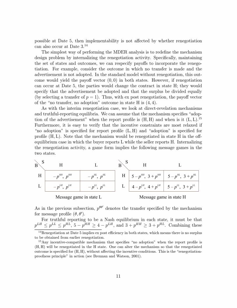
The simplest way of performing the MDER analysis is to redefine the mechanismdesign problem by internalizing the renegotiation activity. Specifically, maintainingthe set of states and outcomes, we can respecify payoffs to incorporate the renego-tiation. For example, consider the outcome in which no transfer is made and theadvertisement is not adopted. In the standard model without renegotiation, this out-come would yield the payoff vector (0, 0) in both states. However, if renegotiationcan occur at Date 5, the parties would change the contract in state H; they wouldspecify that the advertisement be adopted and that the surplus be divided equally(by selecting a transfer of p = 1). Thus, with ex post renegotiation, the payoff vectorof the “no transfer, no adoption” outcome in state H is (4, 4).As with the interim renegotiation case, we look at direct-revelation mechanisms

and truthful-reporting equilibria. We can assume that the mechanism specifies “adop-tion of the advertisement” when the report profile is (H,H) and when is it (L,L).15

Furthermore, it is easy to verify that the incentive constraints are most relaxed if“no adoption” is specified for report profile (L,H) and “adoption” is specified forprofile (H,L). Note that the mechanism would be renegotiated in state H in the off-equilibrium case in which the buyer reports L while the seller reports H. Internalizingthe renegotiation activity, a game form implies the following message games in thetwo states.

– , p pHH HH – , p pHL HL

– , p pLH LH – , p pLL LL

5 – , 3 + p pHH HH 5 – , 3 + p pHL HL

4 – , 4 + p pLH LH 5 – , 3 + p pLL LL

H

L

H L H L

H

L

BS

BS

Message game in state L Message game in state H

As in the previous subsection, pθθ denotes the transfer specified by the mechanismfor message profile (θ, θ ).For truthful reporting to be a Nash equilibrium in each state, it must be that

pLH ≤ pLL ≤ pHL, 5 − pHH ≥ 4 − pLH , and 3 + pHH ≥ 3 + pHL. Combining these14Renegotiation at Date 5 implies ex post efficiency in both states, which means there is no surplus

to be obtained from earlier renegotiation.15Any incentive-compatible mechanism that specifies “no adoption” when the report profile is

(H,H) will be renegotiated in the H state. One can alter the mechanism so that the renegotiatedoutcome is specified for (H,H), without affecting the incentive conditions. This is the “renegotiation-proofness principle” in action (see Brennan and Watson, 2001).

11

inequalities yieldspLL + 1 ≥ pHH ≥ pLL.

The set of implementable state-contingent value functions for the MDER program isthus:

v :{H,L}→ R2 v(L) = (α,−α), v(H) = (5 + α− β, 3− α+ β),

for any α ∈ R and β ∈ [0, 1] . (2)

Note that the opportunity to renegotiate at Date 5, specifically following out-of-equilibrium message profiles, causes a refinement in the set of implementable valuesrelative to the case of interim renegotiation.

Trade Decisions as Options

Everything that the mechanism design program identifies to be implementablecan be achieved, in practice, with forcing contracts. However, there is no reason toexpect that parties would limit themselves to forcing contracts and, therefore, thereis no reason to limit our theoretical analysis to such contractual forms. I next showthat, when there is ex post renegotiation, the set of implementable values significantlyexpands when parties depart from forcing contracts and, instead, use trade decisionsas options.Suppose that at Date 1 the parties write the following contract: If the buyer

adopts the advertisement, then he must pay p +β to the seller; if the buyer does notadopt, then he pays p ; further, the external enforcer is instructed to ignore messagessent at Date 4. For β ∈ (0, 5), this is not a forcing contract–that is, it neithercompels the buyer to adopt the advertisement in both states, nor compels the buyerto not adopt the advertisement in both states. Instead, this is an option contract,but one that uses the buyer’s trade decision, rather than the buyer’s message, as theway to exercise the option. With β ∈ [0, 5], the buyer has the incentive to adopt theadvertisement in state H and not to adopt in state L. From Date 6, this contractyields a payoff vector of (5 − p − β, 3 + p + β) in state H and (−p , p ) in stateL. Because the contract leads to the efficient trade decision in each state, it wouldnot be renegotiated at either Date 5 or Date 3. The contract thus implements value(5− p − β, 3 + p + β) in state H and (−p , p ) in state L.Clearly, by using the trade decision as an option, the parties are able to reduce

the detrimental effect of renegotiation at Date 5. Because the trading opportunity isnondurable, there is no way for the parties to reverse it through renegotiation afterDate 6. The parties could use a more complicated contract that involves transferscontingent on both trade decisions and messages. However, in this example, more

12

complicated contracts cannot improve on the scope of the simple option scheme de-scribed in the preceding paragraph. Thus, the set of implementable state-contingentvalue functions in the case of ex post renegotiation is:

v :{H,L}→ R2 v(L) = (α,−α), v(H) = (5 + α− β, 3− α+ β),

for any α ∈ R and β ∈ [0, 5] . (3)

Preliminary Comments on Ex Post Renegotiation

With the results of the example in hand, it is worthwhile to take stock and reflecta bit before proceeding with the general analysis.Note that, in the case of ex post renegotiation, there is a discrepancy between

the set of implementable value functions and the strictly smaller set identified by theMDER program. The MDER program misses how trade decisions can be used asoptions, precisely because the MDER program treats trade decisions as part of theabstract, public “outcome.”16 For this reason, we should reject the MDER programas incorporating implicit assumptions about contractual incompleteness. We shouldinstead focus on structured models that incorporate the technology of trade andenforcement, and, where appropriate, on the MDIR program.In response to my assertion, a mechanism design theorist might be inclined to

conclude that I am mis-applying the MDER program. The theorist would argue that,if we think the trading opportunity is nondurable (and so trade decisions can be usedas options without being reversed by renegotiation), then the set of implementablevalues is actually characterized by the MDIR program. Segal and Whinston (2000)and others take this position. However, the argument is flawed in two respects.First, the MDIR program actually does not characterize the set of implementable

value functions for the case of renegotiation at Date 5. Comparing Expressions 1and 3, the MDIR program supports β numbers between −3 and 5, while only num-bers between 0 and 5 can be supported with ex post renegotiation. The problem isthat, in designing option contracts, the fixed technology of trade is not as flexible asare messages. Thus, neither the MDER nor the MDIR programs accurately modelthe masonry example with ex post renegotiation. The renegotiation opportunity, ina sense, occurs “in the middle of the mechanism.” To analyze this renegotiation op-portunity, one must examine the structured model that explicitly accounts for thetechnology of trade and external enforcement. In fact, mechanism design method-ology is applicable, but it relies on precise modeling of the technology of trade. Inparticular, one cannot view the “outcome” as merely a specification of the transfer

16This suggests a more nuanced view of Bernheim and Whinston’s (1998) “strategic ambiguity,”whereby external enforcement can mold incentives without forcing any particular action profile.

13

and the trade decision. Rather, an “outcome” must indicate the trade decisions andtransfers that result in the different states, given the technology of trade and theinstructions for the external enforcer. My general model makes this formal.Second, if one argues that the MDER program is inappropriate for settings with

nondurable trading opportunities, one still must justify applying the program to set-tings with durable trading opportunities. You might think that the MDER programcharacterizes settings in which trade decisions are reversible–for example, a gooddelivered at time t can be returned at some future date t–and where renegotiationcan occur between times at which trade decisions can be made and reversed. How-ever, if trade decisions can be made at times t and t then the parties should be ableto write a long-term contract that covers both times. Thus, we still have a settingof “renegotiation within the mechanism” and we still need a structured model to ac-count for the timing of trade decisions and renegotiation opportunities. My generalmodel incorporates these dynamic features and, as I prove in Section 5, it confirmsin general the failure of the MDER program to describe reality.

2 The Main Ingredients of

the General Framework

In this section, I describe in detail the main components of my general model ofcontract. Relative to the example of Section 1, the general model has an arbitrarytrading technology and it also adds the following elements: (i) a verifiable, publicrandom variable, (ii) additional renegotiation opportunities, and (iii) an externallyenforced “continuation value,” which I use to model durability of the trading oppor-tunity. The analysis in this section and the next assumes a fixed set of continuationvalue functions. This set is treated as endogenous in Sections 4 and 5.There are two contracting parties, whom I call “players.” Unverifiable events are

captured by the state θ, which I assume is an element of some set Θ. In the relation-ship’s trading and enforcement phase, the players make verifiable trade decisions andthe external enforcer compels transfers and a state-contingent continuation value.The trade decisions are represented as a ∈ A. The externally enforced transfer isdenoted y = (y1, y2), where yi is the monetary transfer to player i. I assume y ∈ R2

0,where

R20 ≡ {y ∈ R2 | y1 + y2 = 0}.

Regarding the justification for such “balanced transfers,” recall footnote 10. Thecontinuation value function is given by x :Θ→ R2. I assume that x is an element ofsome set X and that, for every θ ∈ Θ, max{x1(θ) + x2(θ) | x ∈ X} exists.The players receive payoffs as a function of the state and the outcome of the

trading and enforcement phase. I assume that the payoffs are additive in money,

14

Players establish a contract.Unverifiable events determine the state, .θ

[Possible renegotiation of the contract.]Players send verifiable messages, m.

[Possible renegotiation of the contract.]Players observe a public random variable, .q

External enforcer compels a transfer, , and the continuation value function, .

yx

Date 1234567

Players make verifiable trade decisions, .a8910

[Possible renegotiation of the contract.]

[Possible renegotiation of the contract.]

Trading/enforcement

phase

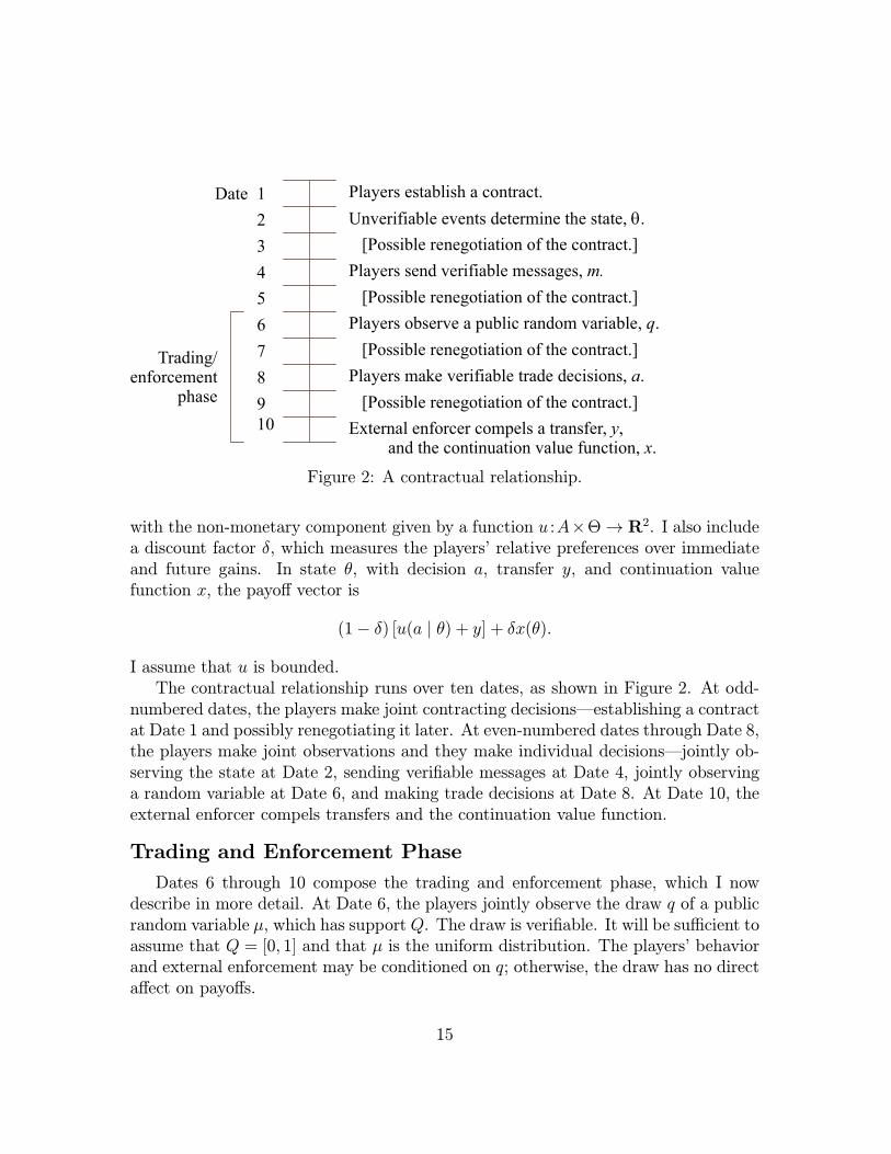
Figure 2: A contractual relationship.

with the non-monetary component given by a function u :A×Θ→ R2. I also includea discount factor δ, which measures the players’ relative preferences over immediateand future gains. In state θ, with decision a, transfer y, and continuation valuefunction x, the payoff vector is

(1− δ) [u(a | θ) + y] + δx(θ).

I assume that u is bounded.The contractual relationship runs over ten dates, as shown in Figure 2. At odd-

numbered dates, the players make joint contracting decisions–establishing a contractat Date 1 and possibly renegotiating it later. At even-numbered dates through Date 8,the players make joint observations and they make individual decisions–jointly ob-serving the state at Date 2, sending verifiable messages at Date 4, jointly observinga random variable at Date 6, and making trade decisions at Date 8. At Date 10, theexternal enforcer compels transfers and the continuation value function.

Trading and Enforcement Phase

Dates 6 through 10 compose the trading and enforcement phase, which I nowdescribe in more detail. At Date 6, the players jointly observe the draw q of a publicrandom variable µ, which has support Q. The draw is verifiable. It will be sufficient toassume that Q = [0, 1] and that µ is the uniform distribution. The players’ behaviorand external enforcement may be conditioned on q; otherwise, the draw has no directaffect on payoffs.

15

At Date 8, the players make inalienable trade decisions, which I assume are si-multaneous and independent. Player i selects ai ∈ Ai. Thus, A = A1 ×A2. I assumeA is finite. The trade decisions are verifiable.At Date 10, the external enforcer compels the transfer y and the continuation

value function x. These are conditioned on the verifiable draw q, on the verifiabletrade decision a, and on the message profile m, as specified by the players’ contract.To focus on interaction in the trading and enforcement phase, at this point I take themessage profile as fixed. Thus, I write y = y(q, a) and x = x(q, a) as the transfer andthe continuation value function that are specified by the contract for the contingencyin which q is the draw and a is the trade profile. The functions y and x are calledthe externally enforced components of the players’ contract.I shall, without loss of generality, ignore the possibility of renegotiation at Dates 7

and 9. Because players are risk-neutral, the effects of allowing renegotiation at Date 7(just after draw q) are identical to the effects of allowing it only at Date 5 (justbefore draw q), which I study in the next section. The justification behind ignoringrenegotiation at Date 9 at this point is that it will be covered by the analysis inSections 4 and 5.17

Given the state θ and the draw q, the externally enforced components of thecontract define a trading game, where the space of action profiles is A and the payoffsare given by

(1− δ) [u(· | θ) + y(q, ·)] + δx(q, ·)(θ).I focus on pure strategy Nash equilibria of the trading game. Let a(q, θ) denote theequilibrium action profile that is chosen by the players in state θ following draw q.Taking the expectation over the random draw, the players’ expected payoff vector instate θ is given by

w(θ) ≡ {(1− δ) [u(a(q, θ) | θ) + y(q, a(q, θ))] + δx(q, a(q, θ))(θ)} dµ(q). (4)

The function w thus gives the state-contingent payoff vectors that can be achieved bythe appropriate choice of the externally enforced components y and x and equilibriumselection a.I use the term outcome for any function from Θ to R2. Think of an outcome,

therefore, as a state-contingent payoff that results from interaction in the tradingand enforcement phase; this should be differentiated from the “trade outcome,” whichonly describes the physical trade decision and monetary transfer. The function w thatis defined above is an outcome.Forcing contracts work in this general model just as they did in the example. For

instance, suppose the players want to have continuation value function x∗ and theywant to force themselves to play action profile a∗, regardless of the state. This can17See the last paragraph in Section 4.

16

accomplish by specifying x and y as follows. First, let x(q, a) ≡ x∗ for all q and a.Second, let L be an upper bound on |ui(a | θ)|, for i = 1, 2. Then, to induce a∗, onecan define y so that (i) for each a = (ai, a

∗j) for which ai = a

∗i , we have yi(q, a) = −L

and yj(q, a) = L; and (ii) y(q, a) = (0, 0) for every other profile a, for all q. Thatis, each player is punished for not taking his part of the prescribed trade action.Obviously, then, a∗ is the only Nash equilibrium of the trading game, in every state.

Definition 1: Externally enforced components y and x are called forcing if, forevery q, there is a unique Nash equilibrium of the trading game A, (1 − δ)[u(· |θ) + y(q, ·)] + δx(q, ·)(θ) and this equilibrium is independent of the state.

Let W (X, δ) be defined as the set of achievable outcomes, given X and δ, andlet W F (X, δ) be the subset of W that can be supported using externally enforcedcomponents that are forcing. That is,

Definition 2: The setW (X, δ) contains w if and only if there are contracted transferand continuation value functions y and x, and there is a function a :Q × Θ → A,such that

(i) Equation 4 is satisfied and

(ii) a(q, θ) is a Nash equilibrium of A, (1−δ)[u(· | θ)+y(q, ·)]+δx(q, ·)(θ) ,for every θ ∈ Θ and q ∈ Q.

The set W F (X, δ) contains w if and only if there are forcing components y, and xand a function a :Q×Θ→ A, such that (i) and (ii) are satisfied for every θ ∈ Θ andq ∈ Q.The following lemma identifies a useful property of the setsW (X, δ) andW F (X, δ).

Lemma 1: W (X, δ) andW F (X, δ) are closed under constant transfers. For example,if w ∈W (X, δ) and if α ∈ R2

0 is a constant transfer, then w+α ∈W (X, δ) as well.Proof: The result follows from the fact that one can add a constant transfer

α ∈ R20 to any given function y without altering the players’ incentives in the trading

phase in any state. Q.E.D.

Contracted Mechanisms

The players’ contract specifies a mechanism, which maps messages sent at Date 4to outcomes induced in the trading and enforcement phase.18 The revelation prin-ciple applies in the following sense. We can restrict attention to direct-revelation18One way of describing a mechanism is to explicitly write y as a function of m, q, and a. Equiv-

alently, one can isolate the trading and enforcement phase by writing y as a function of q and a,noting how y induces an outcome in W , and then thinking of the contract as a mapping from themessages to W . I adopt the latter characterization because it minimizes the amount of notationneeded for the analysis.

17

mechanisms, each of which is defined by a message space M ≡ Θ2 and a functionf :M →W (X, δ). With such a mechanism, at Date 4 the parties simultaneously andindependently report the state. For any report profile m, the mechanism specifiesan element f(m) ∈ W (X, δ), which then determines the payoffs conditional on thestate. We can concentrate on equilibria of the mechanism in which the parties reporttruthfully.19

Renegotiation

Renegotiation can occur at Dates 3, 5, 7, and 9, depending on what one assumes. Ihave already addressed renegotiation at Dates 7 and 9, so now I focus on renegotiationat Dates 3 and 5. We can think of these times as possible opportunities for the playersto discard their originally specified f mapping and replace it with another mapping f .I model renegotiation by supposing that the players divide the renegotiation surplusaccording to fixed bargaining weights π1 and π2, which are nonnegative and sum toone. The generalized Nash bargaining solution and several other common bargainingsolutions have this representation.To be more precise, define

γ(θ, X, δ) ≡ maxw∈W (X,δ)

w1(θ) + w2(θ),

which is the maximal joint payoff that can be obtained in state θ. This joint payoffcan also be written

γ(θ, X, δ) = (1− δ)maxa∈A

[u1(a | θ) + u2(a | θ)] + δmaxx∈X

[x1(θ) + x2(θ)],

because it can be achieved by using a forcing contract. An outcome w is calledefficient in state θ if w1(θ) + w2(θ) = γ(θ,X, δ); otherwise, the outcome is inefficientin state θ.Suppose the original mechanism (M,f) would lead to outcome w in state θ. If

w is inefficient in state θ, then the players have a joint incentive to renegotiate themechanism. The renegotiation surplus is

r(w, θ,X, δ) ≡ γ(θ, X, δ)− w1(θ)− w2(θ).

The players will select a new mapping f that induces an efficient outcome. Further,the surplus will be divided according to the players’ bargaining weights, so thatplayer i obtains wi(θ) + πir(w, θ, X, δ).

19Regarding multiplicity of equilibria, recall footnote 13.

18

3 Implementation Conditions Given X

A state-contingent value function is a function v : Θ → R2 that gives the players’expected payoff vector from the start of Date 3, as a function of the state. The players’contractual objective is to implement the particular function v of their choice. In thissection, I define and characterize the set of implementable value functions, given afixed set of continuation value functions X. I group the analysis into three categories,distinguished by whether the players have the opportunity to renegotiate at Dates 3and 5. The characterization lemmas in this section are all straightforward variationsof well-known theorems from the contract theory literature–in particular, due toMaskin (1999), Maskin and Moore (1999), and Moore and Repullo (1988). I providethe proofs of the first two lemmas; the others are proved similarly.

No Renegotiation

First consider the setting in which the players cannot renegotiate. A mechanism(M, f) implies, for each state θ, a message game in which the players engage at Date 4.The message game has action profiles given by M and payoffs defined by f(·)(θ). Forthis setting, implementability is defined as follows.

Definition 3: A mechanism (M, f) is said to implement value function v if, foreach state θ, there is an equilibrium of the message game that leads to the payoffvector v(θ). Value function v is said to be implementable if there is a mechanismthat implements it.

Let ΛN(X, δ) be the set of implementable value functions, under the assumptionthat the players cannot renegotiate.

Lemma 2: v ∈ ΛN(X, δ) if and only if (i) for every θ ∈ Θ, there is an outcomewθθ ∈ W (X, δ) such that wθθ(θ) = v(θ); and (ii) for every pair of states θ, θ ∈ Θ,there is an outcome wθθ ∈W such that v1(θ ) ≥ wθθ1 and v2(θ) ≥ wθθ

2 .

Proof: For any direct-revelation mechanism (Θ2, f), define wθ1θ2 ≡ f(θ1, θ2) forall θ1, θ2 ∈ Θ. Observe that truthful reporting is a Nash equilibrium if and only ifwθθ1 ≥ wθ1θ1 and wθθ2 ≥ wθθ22 , for every θ ∈ Θ and all θ1, θ2 ∈ Θ. Combining this factwith the definition of implementability produces the result. Q.E.D.

Interim Renegotiation

Next consider the setting in which renegotiation is possible at Date 3 but not atDate 5. In other words, the players can renegotiate between the time that they jointlylearn the state and when the message game is played. In this setting, implementabilityrequires an additional condition–that the equilibrium of the message game is efficientin every state. Let ΛI(X, δ) denote the set of implementable value functions whenthere is interim renegotiation.

19

Lemma 3: v ∈ ΛI(X, δ) if and only if (i) v1(θ)+ v2(θ) = γ(θ,X, δ) for every θ ∈ Θ;and (ii) for every pair of states θ, θ ∈ Θ, there is an outcome wθθ ∈ W (X, δ) suchthat v1(θ ) ≥ wθθ1 and v2(θ) ≥ wθθ

2 .

Proof: First note that v ∈ ΛI(X, δ) implies v1(θ) + v2(θ) = γ(θ, X, δ) for everyθ ∈ Θ. This is because if, at Date 3, the players anticipate getting an inefficientoutcome in a given state, then they would renegotiate the mechanism to obtain anefficient outcome. Next note that, if a state-contingent value function v satisfiesv1(θ) + v2(θ) = γ(θ,X, δ), then there is an outcome wθθ ∈ W (X δ) such that wθθ1 =v1(θ) and w

θθ2 = v2(θ). This follows from Lemma 1. Furthermore, observe that the

players cannot gain from renegotiating at Date 3 in state θ if they anticipate thattheir messages will lead to an efficient outcome. Given these facts, the proof followsthe same steps used to prove Lemma 2. Q.E.D.

Ex Post Renegotiation

Finally, consider the case in which renegotiation is possible at Date 5–betweenthe time the players send messages and the beginning of the trading and enforcementphase. The idea is that the players interact in the contracted mechanism, which leadsto an outcome w. But then, just before the outcome would be induced, the playerscan renegotiate to obtain a different outcome. In this setting, renegotiation impliesefficient outcomes in every state and after every message profile in the mechanism.To characterize implementability for this setting, we must incorporate renegotia-

tion into the definition of an outcome. The set of ex post renegotiation outcomes isdefined as

Z(X, δ) ≡ z :Θ→ R2 there is an outcome w ∈W (X, δ)

such that z(θ) = w(θ) + πr(w, θ,X, δ) for every θ ∈ Θ .

An ex post renegotiation outcome is a state-contingent payoff vector that resultswhen, in every state, the players renegotiate from an outcome in W (X, δ). One cananalyze mechanism design in the setting of ex post renegotiation by simply replacingW (X, δ) with Z(X, δ)–that is, by thinking of the mechanism as a mapping from Mto Z(X, δ), rather than a mapping from M to W (X, δ). If we constrain attention toforcing contracts, then the set of ex post renegotiation outcomes is

ZF (X, δ) ≡ z :Θ→ R2 there is an outcome w ∈W F (X, δ)

such that z(θ) = w(θ) + πr(w, θ, X, δ) for every θ ∈ Θ .

Note that all elements of Z and ZF are efficient in every state.

20

Let ΛEP (X, δ) be the set of implementable value functions when there is ex postrenegotiation and let ΛEPF (X, δ) be the subset of value functions that are sup-ported using forcing contracts. The popular MDER program studies precisely theset ΛEPF (X, δ). As discussed in Section 1, this program identifies ΛEPF (X, δ) ratherthan ΛEP (X, δ) since it treats trading decisions as alienable and public.

Lemma 4: v ∈ ΛEP (X, δ) if and only if (i) for every θ ∈ Θ, there is an outcomezθθ ∈ Z(X, δ) such that zθθ(θ) = v(θ); and (ii) for every pair of states θ, θ ∈ Θ, thereis an outcome zθθ ∈ Z(X, δ) such that v1(θ ) ≥ zθθ1 and v2(θ) ≥ zθθ2 .

Lemma 5: v ∈ ΛEPF (X, δ) if and only if (i) for every θ ∈ Θ, there is an outcomezθθ ∈ ZF (X, δ) such that zθθ(θ) = v(θ); and (ii) for every pair of states θ, θ ∈ Θ,there is an outcome zθθ ∈ ZF (X, δ) such that v1(θ ) ≥ zθθ1 and v2(θ) ≥ zθθ2 .

4 Durability of the Trading Opportunity

Many contractual relationships have durable trading opportunities. For example, aretail firm may contract with a computer software company to design and installspecialized software for inventory control. The software will generate for the retailera flow of value over time, starting as soon as the software is installed. Suppose thesoftware can be installed as early as in January; furthermore, if the seller fails toinstall the software in January, it can still be installed in February, or March, orlater. However, if it is installed in, say, March, then the buyer will not obtain thevalue of the software in January or February.Durability implies that the trade decisions are at least partially reversible. For

example, the seller’s decision not to install the software in January can be reversedby installing the software in February. Sometimes, trade decisions are fully reversible.For instance, if the seller installs the software in January, then perhaps the softwarecan be uninstalled at any future time.This section concerns contractual settings with durable, fully reversible trading

opportunities. To model durability and reversibility, I suppose that the players in-teract over an infinite number of discrete “periods,” starting in Period 1.20 In each

20Jackson and Palfrey (2001) analyze a dynamic model that is, on first glance, similar to theone I study here. Their model differs in important respects, however. It assumes that players canunilaterally impose a default decision in each period, which gives players more power than would beappropriate for a model of most contractual settings. It also abstracts from inalienable trade deci-sions, durability, and reversibility. Interestingly, though, the proof of their result for nondiscountedenvironments has a stationarity feature that foretells of the importance of stationarity in my model.For another interesting, but less related, modeling exercise, see Kalai and Ledyard (1997). MacLeodand Malcomson’s (1993) basic model also has a dynamic trading opportunity but they focus on sta-tionary contracts; these authors also examine a multi-period contracting environment with a statevariable that follows a Markov process, and again impose a restriction on the class of contracts.

21

period, play proceeds as in Figure 2: the players send messages as prescribed by acontractual mechanism, the players make trade decisions, and the external enforcercompels the transfers that the players’ contract prescribes. The state, which is real-ized at Date 2 of Period 1, is fixed for the entire game. Thus, Dates 1 and 2 occuronly in Period 1; these dates are skipped in all other periods.Preferences are given by the discounted and normalized sum of per-period payoffs,

calculated using discount factor δ. Thus, in state θ, the payoff vector from Date 3 inPeriod 1 is

(1− δ)∞

t=1

δt−1 u(at | θ) + yt ,

where {at, yt}∞t=1 denotes the sequence of trade decisions and monetary transfers. Irepresent reversibility by assuming that the trade decision that is taken in one perioddoes not constrain trade decisions taken in succeeding periods and it has no directeffect on the payoffs in future periods. For example, if the players make trade decisiona in the current period, then they can reverse it by selecting any other trade decisiona in the next period. An infinite sequence of trade decision a means that a is neverreversed. The discount factor measures the degree of durability; setting δ close to 1means a highly durable trading opportunity, whereas the opposite is captured with δclose to 0.The players can write long-term contracts that condition the transfer in a given

period on the entire verifiable history–messages, trade decisions, and draws in thecurrent period and in previous periods. From a given period, a contract’s implicationsfor the future can be summarized by the implied continuation value function. Thus,instead of keeping track of the transfers a contract prescribes for future periods (aswell as the induced behavior), one can simply specify the continuation value function.Because the contracting environment is stationary (due to reversibility), the set offeasible continuation value functions is independent of the reference period and isequal to the set of implementable value functions. That is, X will give the set ofpossible state-contingent payoffs from Date 3 in any period; for Period 1 in particular,X is the set of implementable value functions. To analyze long-term contracts, Itherefore adopt a recursive formulation, whereby X is endogenously determined.To identify the set of implementable value functions, a fixed point condition is

added to the analysis from preceeding sections. Borrowing a term from Abreu, Pearce,and Stacchetti (1986), I say that a set X of value functions has the self-generationproperty with respect to ΛN if X ⊂ ΛN (X, δ). Self-generation with respect to ΛI ,ΛEP , and ΛEPF are defined analogously. Let V N(δ), V I(δ), V EP (δ), and V EPF (δ)be the sets of implementable value functions for the settings of, respectively, norenegotiation, interim renegotiation, ex post renegotiation, and ex post renegotiationwith forcing contracts.

22

Definition 4: V N (δ) is defined as the maximal set of value functions that has theself-generation property with respect to ΛN . V I(δ), V EP (δ), and V EPF (δ) are definedas the maximal sets of value functions that have the self-generation property withrespect to ΛI , ΛEP , and ΛEPF , respectively.

This definition completes the construction of my general modeling framework.I conclude this section with a two comments on the general model. First, note

that any setting with a nondurable trading opportunity, including the example inSection 1, can be analyzed as a special case of the general model with δ = 0.Second, I wish to expound on the possibility of renegotiation at Date 9, an issue

of which I earlier deferred discussion. Having renegotiation at Date 9 is equivalentto assuming that renegotiation can occur at Date 3. This is because, given balancedtransfers, the only way for the players to realize a joint gain through renegotiationat Date 9 is to alter the continuation value function. The continuation value in oneperiod is just the discounted value from the start of the next period, so renegotiationat the end of one period has the same effect as does renegotiation at the start ofthe next period. Note that my analysis does leave out one case: that in which non-balanced transfers are allowed and the players never can renegotiate. I have notincluded this case because it seems unrealistic and uninteresting and, furthermore, itis simple to analyze.

5 Characterization Results

In this section, I partially characterize and compare the sets V N(δ), V I(δ), V EP (δ),and V EPF (δ). The results presented in this section are proved in the Appendix.

Existence and Inclusion

I begin with an existence result.

Theorem 1: V EPF (δ), V EP (δ), V I(δ), and V N(δ) are well-defined and non-empty.

Existence is proved by finding a set that has the self-generation property and thenrecognizing that the Λ mappings are monotone.To get an idea of what the implementable sets contain, note that they are bounded

in thatv1(θ) + v2(θ) ≤ max

a∈A[u1(a | θ) + u2(a | θ)]

for every v ∈ V N(δ) ∪ V I(δ) ∪ V EP (δ) ∪ V EPF (δ). This is because the joint valuev1(θ)+v2(θ) is achieved by a discounted sequence of trade decisions and, furthermore,balanced transfers do not affect the joint value. In fact, the upper bound is attained.

23

For example, consider the case of ex post renegotiation with forcing contracts andsuppose the players agree to a contract that forces them to select some arbitrarytrade decision a in each period. Then if a is inefficient in the actual state, theplayers will renegotiate their contract so that an efficient trade decision is selected.Thus, if v ∈ V EPF (δ) then

v1(θ) + v2(θ) = maxa∈A

[u1(a | θ) + u2(a | θ)]

for every state θ. This result also holds for the sets V EP (δ) and V I(δ). In theAppendix, I formalize this analysis in terms of the Λ mappings.The following extension of Lemma 1 shows that the players can freely divide value

in ways that are constant across states.

Lemma 6: The sets V N(δ), V I(δ), V EP (δ), and V EPF (δ) are all closed under con-stant transfers.

For example, take any v ∈ V I(δ) and a constant α ∈ R20, and define v :Θ → R2 so

that v (θ) = v(θ) + α for each θ ∈ Θ. Then v ∈ V I(δ) as well.The next result ranks the sets of implementable value functions by inclusion. The

result confirms in general what the example in Section 1 demonstrated.

Theorem 2: V EPF (δ) ⊂ V EP (δ) ⊂ V I(δ) ⊂ V N(δ) and, in general, none of thesesets are equal.

In words, interim renegotiation restricts the set of implementable state-contingentvalue functions. Ex post renegotiation implies a further restriction. Limiting atten-tion to forcing contracts implies still a smaller set.

Stationarity and Durability

I next report my main results, which establish the efficacy of stationary contractsand the relation between durability and implementation. For the definition of sta-tionary contracts, let P(R2) denote the set of subsets of R2.

Definition 5: Take as given a function Λ∗ : P(R2) × [0, 1) → P(R2). A state-contingent value function v is called supported by a stationary contract withrespect to Λ∗ and δ, if v ∈ Λ∗({v}, δ).In other words, stationarity means v can be supported by a contract that specifies thesame continuation value function (that is, itself) in the following period, regardlessof behavior in the current period. If this is the case, the transfer function y can bechosen to condition only on the verifiable events of the current period. Stationarycontracts are thus simple in that they can be expressed as the repeated applicationof a short-term contract.

24

An issue of both practical and theoretical interest is the extent to which nonsta-tionary contracts can improve on the scope of stationary contracts. For example, bymaking the continuation value function depend on the players’ behavior, it may bepossible to support a wider range of state-contingent values than can be done oth-erwise. Surprisingly, for most of the settings I analyze, nonstationary contracts offerno advantage.

Theorem 3: In all settings, except possibly in the case of ex post renegotiation, allimplementable value functions are supported by stationary contracts. More precisely,for each k ∈ {EPF, I,N} and every δ ∈ [0, 1), every value function v ∈ V k issupported by a stationary contract with respect to Λk and δ.

The intuition behind this theorem runs as follows. Constrain attention to forcingtransfers (which is justified when k = EPF , k = I, or k = N) and ex post or interimrenegotiation. Suppose we have a long-term contract that implements value functionv. Contingent on message profile m sent in the first period, the contract specifiesa distribution over trade outcomes in the first period and continuation values fromthe start of the second period. Because of renegotiation, the continuation valuesare efficient in every state. Thus, renegotiation in the first period can be viewedas adjusting the first-period trade outcome, while keeping the continuation valuesunchanged.Applying this logic to characterize the continuation values from Period 2, Period 3,

and so on, we can write v in terms of a random sequence of trade outcomes over time,from which the players renegotiate. The sequence of trade outcomes depends onlyon the message profile m, while renegotiation also depends on the actual state θ. Astationary contract can achieve the same state- and message-contingent payoffs byspecifying a random trade outcome that, repeated each period, matches the randomsequence of trade outcomes. The construction relies on the random draw q. Sucha construction may not be possible in the case of ex post renegotiation without theconstraint to forcing transfers because, when using trade decisions as options, theplayers’ incentives at Date 8 are sensitive to the continuation values.On the applied side, this theorem establishes that optimal contracts can always

take a very simple, stationary form, whereby the players interact in the same way ineach period. On the technical side, the theorem shows that the analysis of long-termcontracting reduces to selecting a one-period mechanism that is repeated over time.That is, players choose a long-term contract that requires them to play the sameshort-term mechanism in each period.Theorem 3 leads to

Theorem 4: V EPF (δ), V I(δ), and V N (δ) are all constant in δ.

This result states that, except possibly for the case of ex post renegotiation, theset of implementable value functions does not depend on the degree to which the

25

trading opportunity is durable. Thus, we can write V EPF , V I , and V N withoutthe δ argument. The powerful implication for contract analysis is that, for settingswith no renegotiation, interim renegotiation, and ex post renegotiation with forcingcontracts, the dynamic contracting problem reduces to a standard “static” problem(with δ = 0).

Summary

The results of this section can be summarized as follows. Take as given a contrac-tual setting with reversible trade decisions. Note that reversibility is vacuous if thetrading opportunity is nondurable (δ = 0).

(a) Ex post renegotiation: If the players can renegotiate just aftersending messages (at Date 5 in each period), then the set of implementablestate-contingent value functions is V EP (δ). This set generally depends onδ.

(b) Interim renegotiation: If, in each period, the players can renego-tiate before sending messages but not after (that is, at Date 3 but notDate 5), then the set of implementable value functions is V I .

(c) No renegotiation: If the players cannot renegotiate, then the set ofimplementable value functions is V N .

Note that, when there is ex post renegotiation, the implementable set depends on thetechnology of trade and on the discount factor.The results lead to two important conclusions. First, the standard MDIR pro-

gram and the no-renegotiation mechanism-design program are valid to study a widerange of contractual settings. Second, to understand contractual imperfection andimplementability in settings where players can renegotiate ex post, it is critical thatwe explicitly address the technology of trade. The popular MDER program does notaccurately characterize contractual scope. Instead, one must evaluate V EP (δ), whichdepends on the technology of trade and the degree of durability.

6 Two More Examples

To further demonstrate how the proper accounting of the technology of trade im-proves our understanding of contractual imperfections, I present two more examples.The first involves a “cross investment,” whereas the second features a pure “self in-vestment.”

26

Efficient Cross-Investments

Consider a contractual setting with cross investments–which Che and Hausch(1999) call “cooperative investments.”21 A buyer (player 1) and a seller (player 2)contract to trade one unit of an intermediate good; the parties interact over time ina setting of durability and reversibility. At Date 2 in Period 1, the seller makes aninvestment θ ≥ 0, at immediate cost θ, which enhances the buyer’s value of trade.At Date 8 in each period, the buyer can accept or reject delivery of the good.22 If heaccepts then he obtains (1− δ)σ(θ) in the current period, minus any transfer p madeto the seller. In this event, the seller gets p. (I assume the seller’s investment does notaffect his delivery cost, which I normalize to zero.) If the buyer rejects delivery thenboth parties obtain zero in the current period, except for any transfer made betweenthem.I assume that σ is strictly increasing and σ(0) > 0, which means accepting delivery

is always ex post efficient. The efficient investment θ∗ solves maxθ σ(θ)− θ. I assumethe maximum exists and is positive. I also assume that the parties can renegotiateex post (at Date 5) in each period, and that they have equal bargaining weights.This model is a special case of Che and Hausch’s (1999) model of cooperative

investments and ex post renegotiation. Che and Hausch study the forcing contractset V EPF and they show that the hold-up problem severely restricts implementability.In fact, for the model here, they prove that the “null contract”–specifying no trade–is best; further, the parties are doomed to a situation in which the seller invests lessthan θ∗.A very different picture emerges when trade decisions are used as options. In fact,

as shown below, V EP contains the value function v∗ defined by v∗2(θ) = σ(θ∗) for allθ ≥ θ∗ and v∗2(θ) = σ(θ)/2 for θ < θ∗. Remember that this state-contingent valuefunction gives the payoff vector from Date 3 and does not include the sunk investmentcost. With the contract that implements v∗, the seller’s Period 1/Date 2 investmentdecision is to maximize v∗2(θ)− θ. Clearly, the seller optimally selects investment θ∗

and efficiency is achieved.Here is a stationary contract that implements v∗. The parties direct the external

enforcer to, in each period, compel a transfer of (1 − δ)σ(θ∗) from the buyer to theseller if and only if the buyer accepts delivery; otherwise, there is no transfer. Theexternal enforcer ignores the parties’ messages and all behavior in previous periods.Note that, under this transfer function, the buyer will accept delivery in a givenperiod if and only if θ ≥ θ∗.If the seller chooses θ ≥ θ∗ then the parties never renegotiate the contract and the

21I avoid using the term “cooperative” here because I think it can easily be confused with “coop-erative behavior” and can be misleading.22If the buyer accepts delivery in one period and then rejects it in the next, this is interpreted as

the buyer returning the good.

27

buyer accepts delivery in each period. In this case, the seller obtains σ(θ∗) from Date 3of Period 1. On the other hand, if the seller chooses some θ < θ∗ then, anticipatingrejection, the parties will renegotiate. The disagreement point of renegotiation isthe contract’s continuation value v∗, which satisfies v∗1(θ) + v

∗2(θ) = σ(θ). Thus, the

renegotiation surplus is the gain from trade in the current period, or (1 − δ)σ(θ),which the parties divide equally. This division implies that v∗2(θ) = σ(θ)/2.Efficient investment incentives in this example are due to technology of trade. If

some other technology existed, such as if the seller makes the trade decision, thenefficiency may not result and Che and Hausch’s conclusions may, at least partially,reemerge. However, in the least, this example shows that cross investment may notbe as problematic as the literature suggests.

Complexity and Hold-up

Next consider an example with pure self investment, along the lines of Segal (1999)and Hart and Moore (1999). This example will reiterate these authors’ main point–that hold-up problems can exist even in cases of pure self investment–and show thatthe insight is still valid when one properly accounts for the technology of trade. Thedegree of the hold-up problem is sensitive to the technology of trade.A buyer (player 1) and a seller (player 2) contract on a nondurable trading op-

portunity, so δ = 0. As with the previous example, the state represents the seller’sDate 2 investment, which is observed by the buyer but is not verifiable. The sellercan either invest “high,” which yields state H, or invest “low,” yielding state L. Thehigh investment entails a cost c, which is immediately paid by the seller and is notincluded in the u specification below. Low investment is costless. Clearly, the sellerwill have an incentive to invest high only if the difference between what he expectsto obtain in states H and L weakly exceeds c.The buyer makes the trade decision at Date 8, which is either ah or al. The utility

function u is defined by: u(ah | H) = (10, 0), u(al | H) = (22,−22), u(ah | L) = (0, 0),and u(al | L) = (10,−8). Note that this is an example of self investment, because, ifthe optimal trade decision is made (ah in state H, al in state L), the seller’s investmentonly affects his own cost (0 in state H, 8 in state L).23 Assume that c ∈ (0, 8), whichmeans that high investment is efficient. Also assume that the players can renegotiateex post and that the buyer has all of the bargaining power during renegotiation.The analysis of forcing contracts runs as follows. By the revelation principle, one

can focus on contracts that force ah at price pH when the message profile is (H,H),and force al at price pL when the message profile is (L,L). The contract specifies either

23I use the term “self investment” as the literature does, although I would not say that it is anaccurate description of the contracting environment. Although the optimal trade decision has the“self investment” flavor, the seller’s investment affects the buyer’s payoff of the suboptimal tradedecision. Segal (1999) uses the term “complex” to describe such trading environments.

28

ah or al when the message profile is (L,H), that is, when the buyer reports L and theseller reports H. Consider these cases separately.First, suppose that the contract forces ah at price p when the message profile is

(L,H). For truthful reporting to be an equilibrium of the message game in both states,it must be that player 1 has no incentive to send message L in state H and player 2has no incentive to send message H in state L. If player 1 deviates in state H, thenthere would be no renegotiation (because ah is still specified). Player 1 thus reportstruthfully in state H if and only if

10− pH ≥ 10− p.If player 2 deviates in state L, then the players would renegotiate the contractually-specified trade decision, but player 1 would get all of the surplus. Player 2 thusreports truthfully in state L if and only if

pL − 8 ≥ p.Combining the two inequalities yields the constraint pL ≥ pH + 8.Second, suppose that the contract forces al at price p when the message profile

is (L,H). In this case, renegotiation would occur if player 1 reports L in state H, butrenegotiation would not occur if player 2 reports H in state L. Equilibrium conditionsfor the message game are

10− pH ≥ 12− p+ 10and

pL − 8 ≥ p− 8,which simplify to pL ≥ pH + 22.Clearly, then, player 2’s payoff in state L must be at least as high as is his payoff

in state H, which means no forcing contract induces the seller to invest high. Infact, with ex post renegotiation, no contract (forcing or non-forcing) can induce highinvestment.To see why non-forcing contracts cannot improve on forcing contracts in this

example, consider the scope of non-forcing contracts. Suppose that, given a particularmessage profile, the contract specifies a price of ph if the buyer chooses trade decisionah and a price of pl if the buyer chooses trade decision al. This is necessarily a forcingcontract either if pl − ph > 12 (in which case player 1 has the incentive to choose ahin both states) or if pl − ph < 10 (in which case player 1 has the incentive to chooseal in both states). One can easily confirm that if pl − ph ∈ [10, 12] then player 1 hasthe incentive to select ah in state L and to select al in state H. There are no valuesof pl and ph that give player 1 the incentive to select ah in state H and al in state L.Thus, there is only one type of non-forcing contractual provision: that which has

pl− ph ∈ [10, 12]. This leads to payoff vector (22− pl, pl− 22) in state H and (ph, ph)

29

in state L. Suppose that this contractual provision is specified for the message profile(L,H). Then, if (L,H) is sent, the players would renegotiate to obtain the efficienttrade decision. This implies the payoff vector (22 − pl + 10, pl − 22) in state H and(ph + 2, ph) in state L. The equilibrium conditions for the message game are thus

10− pH ≥ 22− pl + 10

andpL − 8 ≥ ph.

Combining these inequalities with pl − ph ∈ [10, 12], we obtain pL ≥ pH + 18. Again,player 2’s payoff in state L must be higher than it is in state H, implying that he doesnot have the incentive to invest high.

7 Conclusion

I have demonstrated that, to appropriately study institutional constraints, the analy-sis of contract must start with an understanding of the technology of trade. Whenparties can renegotiate just before making trade decisions, this technology greatlyaffects implementability. Thus, researchers should take a structured, game-theoreticapproach to studying contract and enforcement. Researchers must be clear aboutexactly what is verifiable, the nature and timing of inalienable decisions, and howexternal enforcement occurs.My analysis here has implications for the applicability of popular mechanism de-

sign models. Some theorists, including Segal and Whinston (2000), have stated thatfuture work in applied contract theory will be geared toward discovering whetherit is the MDER or MDIR program that is the “right” model of any particular set-ting. I find that this objective is in error. The MDER program under-represents thetrue scope of implementability. Contracting parties can often overcome contractualimperfections–to motivate efficient cross investment, for example–even when theyhave the opportunity to renegotiate just before making trade decisions. In settingswith durable trading opportunities and reversibility, parties can effectively deal withthe specter of renegotiation by writing long-term contracts. Finally, I emphasizethat the mechanism design methodology is still applicable and useful, as long as onecorrectly defines the outcome set. Unfortunately, differential methods may be lessapplicable than is currently thought.24

I conclude that the MDER program makes hidden assumptions of contractualincompleteness. It can be justified on the basis of a restriction to forcing contracts or,possibly, by assuming that trade decisions are only partially verifiable. It can also be

24When trade decisions are used as options, we lose the constant-sum condition that underlies theanalysis of Segal and Whinston (2001).

30

justified, in a durability setting, on the basis of a restriction to short-term contracts.By “short-term contracts,” I mean contracts that specify a transfer function for thecurrent period, but specify nothing for future periods (not even that the messagegame and transfer of the current period is repeated in future periods). I can thinkof no ready defense of these incompleteness assumptions, just as I see no reason tobelieve that parties would limit themselves to forcing or short-term contracts.25

I believe that theorists who idealize the “complete contract” view ought to under-stand the contractual incompleteness inherent in their own models. I have nothingagainst the complete contract ideal, in theory, although I find it is not widely ap-plicable. After all, real contracting parties usually face all sorts of technological andinstitutional constraints. Indeed, an opportunity for parties to renegotiate–one thatcannot be controlled by external enforcement–is an incompleteness restriction thatmany scholars find important and that lies at the heart of most recent contract theory.I simply point out that understanding this incompleteness relies on understanding thetechnology of trade.My analysis also has practical relevance. In the least, it should remind us that, to

some extent, messages are a theoretical construct. While we sometimes do observecontracts that require parties to send verifiable messages (in real estate transactions,for example), we also often see option contracts that merely specify transfers onthe basis of productive decisions (in some procurement settings, for example). Wheretrading opportunities are durable, we often observe contracts with stationary terms.26

There are myriad promising opportunities for fruitful research on contracting withinstitutional constraints. Given the importance of the technology of trade, the analy-

25My message can be further illustrated in the context of Edlin and Hermalin’s (2000) debate withNoldeke, G. and K. Schmidt (1998). In their discussion of whether a party could let an option expireand then renegotiate from scratch, Edlin and Hermalin appeal to the “outside option principle,”whereby the outside option implies an inequality constraint on the outcome of negotiation ratherthan serving as the disagreement point. While there are bargaining models that justify treatingoutside options in this way, these models blur the distinction between verifiable trade decisionsand noncontractible renegotiation opportunities. If parties can exercise trade-based options in theprocess of renegotiating, then either trade decisions are really not fully verifiable or the opportunityto renegotiate can be partially controlled by the external enforcer (because he can observe a party’sactions whenever an option can be exercised–which, for example, would be in every round of analternating-offer bargaining game). Edlin and Hermalin may have one of these justifications in mind,or they may be thinking of an institutional constraint that limits the time in which an option may beexercised. In any case, I assert that one must model the timing of renegotiation and trade in orderto understand exactly what is being assumed. Note that, in my framework, the non-contractiblerenegotiation opportunity is separated in time from the verifiable trade decisions, so that a partycannot delay the trading opportunity by refusing to make an agreement at the time of renegotiation.Other modeling approaches may be useful for comparison.26For example, many construction contracts include a term such as “The contractor’s fee is reduced

by $X for every day following date Y that he fails to complete the project.” The law recognizeslong-term contracts just as it does shorter-term ones.

31

sis of specific contractual settings seems in order. Further, the notions of durabilityand reversibility deserve extended study. My work on durability reported here onlyaddresses the specialized environment in which trade decisions are fully reversible.We should develop a better understanding of how limited reversibility influences con-tractual scope. Overall, it may be worthwhile to revisit some of the literature’s basicconcepts from a more detailed institutional foundation.27 In conjunction with Watson(2001), which seeks to clarify the notion of contract in games, my general frameworkmay be a good starting point for future work.

27Bull and Watson (2001), for example, study the notion of verifiability as it relates to evidencedisclosure in an enforcement system. Schwartz and Watson (2001) study contract and enforcementwhen contracts are costly to form and renegotiate; they relate the costs to actual legal rules.

32

A Appendix: Proofs

In this appendix, I restate and prove the theorems found in Section 5. I begin withTheorems 1 and 2, which I prove together.

Theorem 1: V EPF (δ), V EP (δ), V I(δ), and V N(δ) are well-defined and non-empty.

Theorem 2: V EPF (δ) ⊂ V EP (δ) ⊂ V I(δ) ⊂ V N(δ) and, in general, none of thesesets are equal.

Proof: First note that Λk is monotone, for all k ∈ {EPF,EP, I,N}. That is,X ⊂ X implies Λk(X , δ) ⊂ Λk(X, δ). This implies that V k(δ) is well-defined, for allk ∈ {EPF,EP, I,N}.Next note that ΛEPF (X, δ) ⊂ ΛEP (X, δ), which follows from ZF (X, δ) ⊂ Z(X, δ).

From Lemmas 2 and 3, we have ΛI(X, δ) ⊂ ΛN(X, δ). The renegotiation-proofnessprinciple (see Brennan and Watson 2001) implies that ΛEP (X, δ) ⊂ ΛI(X, δ). Usingthe monotone property and the definitions of V EPF (δ), V EP (δ), V I(δ), and V N (δ),we have the inclusion statement of Theorem 2. The example analyzed in Section 1proves the claim of unequal sets.To prove that the implementable sets are non-empty in general, let a be an

arbitrary member of A and define v by

v (θ) ≡ u(a | θ) + π maxa∈A

[u1(a | θ) + u2(a | θ)]− u1(a | θ)− u2(a | θ)for every θ. This is the value function that would result if the players renegotiated overthe infinite sequence of trade decisions, with the disagreement point given by decisiona chosen in each period. One can easily confirm (with a contract that forces a andno transfer in the current period, regardless of messages) that v ∈ ΛEPF ({v }, δ),regardless of δ. Thus, {v } has the self-generation property with respect to ΛEPF ,and so V EPF (δ) = ∅. The inclusion property implies that the other sets are alsonon-empty. Q.E.D.

This proof and the discussion in Section 5 make it clear that, for each k ∈{EPF,EP, I,N},

γ(θ, V k(δ), δ) ≡ maxa∈A

[u1(a | θ) + u2(a | θ)].This justifies redefining γ and r as

γ(θ) ≡ maxa∈A

[u1(a | θ) + u2(a | θ)]and

r(w, θ) ≡ γ(θ)− w1(θ)− w2(θ).I use these definitions for the remainder of this appendix. I also state the followinglemma for reference.

33

Lemma 7: If v ∈ V EPF (δ) V EP (δ) V I(δ), then v1(θ) + v2(θ) = γ(θ), for allθ ∈ Θ.To prove Theorems 3 and 4, I use the following four results.

Lemma 8: Suppose v ∈ V EPF (δ) and consider the direct-revelation mechanism thatimplements v in the current period–this mechanism maps message profiles into el-ements of ZF (V EPF (δ), δ). Then for every message profile m ∈ Θ2, there exist dis-tributions α ∈ ∆A and φ ∈ ∆V EPF (δ) such that, for each state θ, the payoff vectorcontingent on m in state θ is

(1− δ)a∈A

[u(a | θ) + πr(u(a | ·), θ)]α(a) + δ v dφ(v ).

In the case of interim renegotiation, the payoff vector can be written

(1− δ)a∈A

u(a | θ)α(a) + δ v dφ(v ),

for some α ∈ ∆A and φ ∈ ∆V I(δ).Proof: Consider any v ∈ V EPF (δ). Contingent on m, in state θ the players obtain

a payoff given by w(θ) + πr(w, θ), where w ∈W F (V EPF (δ), δ) depends on m. Recallthat w(θ) is given by Equation 4 on page 16, for an appropriately defined transferfunction y, a continuation value function x, and a behavior function a. Let φ be thedistribution over V EPF (δ) implied by x(·, a(·, θ)) and µ.From Lemma 7, every v in the support of φ is efficient. Thus, the renegotiation

surplus derives entirely from a gain achieved in the current period. Since the playersdivide this surplus according to their bargaining weights, relative to the disagreementpoint given by w, we can express the payoff vector as:

w(θ) + πr(w, θ) = (1− δ) [u(a(q, θ) | θ) + y(q, a(q, θ)) + πr(u(a(q, θ) | ·), θ)] dµ(q)+δ v dφ (v ). (5)

The first and last terms in the first integral can be written

(1− δ)a∈A

[u(a | θ) + πr(u(a | ·), θ)]α(a),

for some α ∈ ∆A (since the trade decision may be conditioned on q). Regarding thesecond term, define

y ≡ (1− δ) y(q, a(q, θ))dµ(q).

34

Note that y is balanced.From Lemma 6, we know that v + y ∈ V EPF (δ) for every v ∈ V EPF (δ). Thus,

there is a distribution φ ∈ ∆V EPF (δ) such that

δ v dφ(v ) = δ v dφ (v ) + y.

Substituting this into Equation (5) yields the conclusion of the theorem.For the case of interim renegotiation, where v ∈ V I(δ), the proof is simpler.

Lemma 6 allows the externally enforced transfer to be merged into the continuationpayoff. Q.E.D.

Lemma 9: There is a number L such that, for both i = 1, 2, every δ, every two statesθ, θ ∈ Θ, and every v ∈ V I(δ), |vi(θ)− vi(θ )| < L.

Proof: Recalling the definitionW from Section 2, and recalling that u is bounded,we see that there is a number L such that, for both i = 1, 2, every two states θ, θ ∈ Θ,and every w ∈ W , |wi(θ) − wi(θ )| < L . Combining this with the implementationconditions of Lemma 3, it is not difficult to confirm the result. Q.E.D.

Lemma 10: Consider any v ∈ V EPF (δ) V I(δ). For each state θ, there is a se-quence {αt}∞t=1 ⊂ ∆A and a balanced constant transfer yθ such that

v(θ) =∞

t=1

δt−1(1− δ)a∈A

[u(a | θ) + πr(u(a | ·), θ)]αt(a) + yθ.

Proof: First take the case of ex post renegotiation. Recursive application ofLemma 8, using message profile (θ, θ), establishes the following. There are sequences{αt}∞t=1 ⊂ ∆A and {φt}∞t=2 ⊂ ∆V I(δ) such that, for every positive integer T ,

v(θ) =T

t=1

δt−1(1− δ)a∈A

[u(a | θ) + πr(u(a | ·), θ)]αt(a) + δT v dφT+1.

As T → ∞, the summation term converges. Thus, the integral term also converges.Further, because of discounting and bounded utilities, the limit of the integral term,which defines yθ, is balanced.The same argument can be used for the case of interim renegotiation, which has

efficient outcomes in equilibrium. In this case, one can focus on forcing transfersbecause there is no renegotiation at Date 5 in each period. Q.E.D.

35

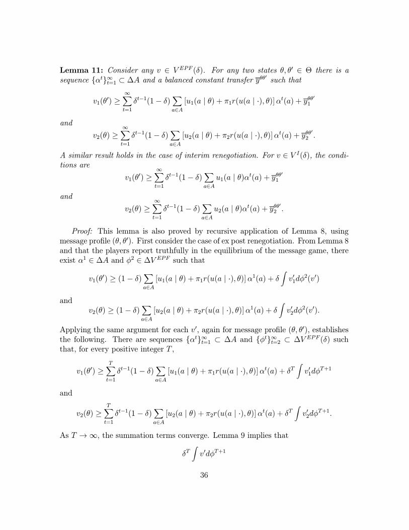
Lemma 11: Consider any v ∈ V EPF (δ). For any two states θ, θ ∈ Θ there is asequence {αt}∞t=1 ⊂ ∆A and a balanced constant transfer yθθ such that

v1(θ ) ≥∞

t=1

δt−1(1− δ)a∈A

[u1(a | θ) + π1r(u(a | ·), θ)]αt(a) + yθθ1

and

v2(θ) ≥∞

t=1

δt−1(1− δ)a∈A

[u2(a | θ) + π2r(u(a | ·), θ)]αt(a) + yθθ2 .

A similar result holds in the case of interim renegotiation. For v ∈ V I(δ), the condi-tions are

v1(θ ) ≥∞

t=1

δt−1(1− δ)a∈A

u1(a | θ)αt(a) + yθθ1and

v2(θ) ≥∞

t=1

δt−1(1− δ)a∈A

u2(a | θ)αt(a) + yθθ2 .

Proof: This lemma is also proved by recursive application of Lemma 8, usingmessage profile (θ, θ ). First consider the case of ex post renegotiation. From Lemma 8and that the players report truthfully in the equilibrium of the message game, thereexist α1 ∈ ∆A and φ2 ∈ ∆V EPF such that

v1(θ ) ≥ (1− δ)a∈A

[u1(a | θ) + π1r(u(a | ·), θ)]α1(a) + δ v1dφ2(v )

andv2(θ) ≥ (1− δ)

a∈A[u2(a | θ) + π2r(u(a | ·), θ)]α1(a) + δ v2dφ

2(v ).

Applying the same argument for each v , again for message profile (θ, θ ), establishesthe following. There are sequences {αt}∞t=1 ⊂ ∆A and {φt}∞t=2 ⊂ ∆V EPF (δ) suchthat, for every positive integer T ,

v1(θ ) ≥T

t=1

δt−1(1− δ)a∈A

[u1(a | θ) + π1r(u(a | ·), θ)]αt(a) + δT v1dφT+1

and

v2(θ) ≥T

t=1

δt−1(1− δ)a∈A

[u2(a | θ) + π2r(u(a | ·), θ)]αt(a) + δT v2dφT+1.

As T →∞, the summation terms converge. Lemma 9 implies that

δT v dφT+1

36

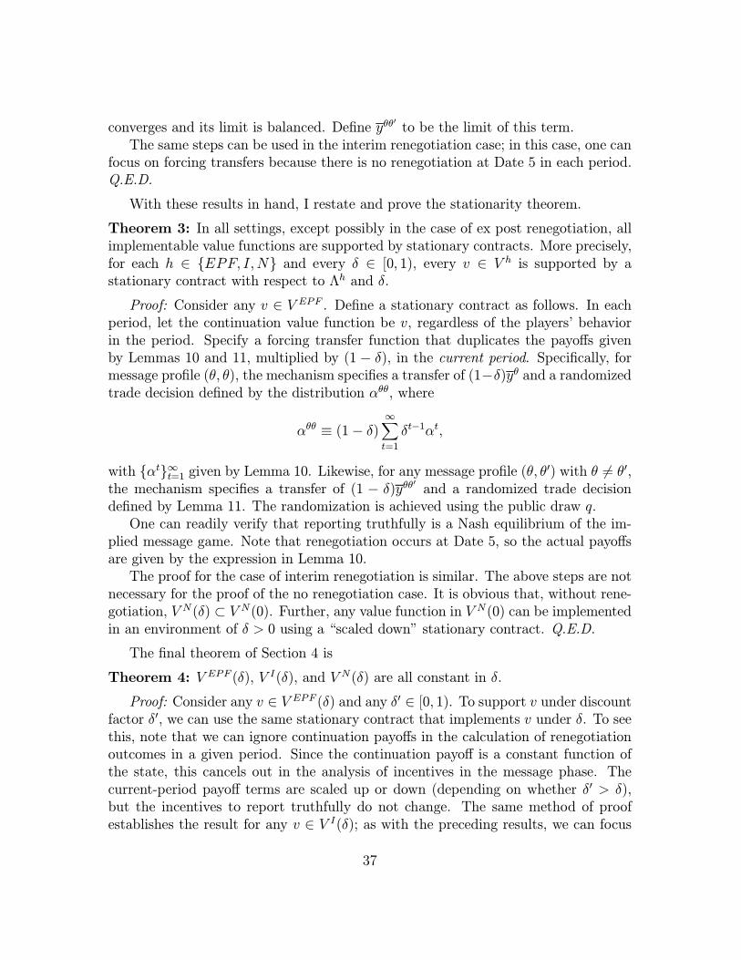
converges and its limit is balanced. Define yθθ to be the limit of this term.The same steps can be used in the interim renegotiation case; in this case, one can

focus on forcing transfers because there is no renegotiation at Date 5 in each period.Q.E.D.

With these results in hand, I restate and prove the stationarity theorem.

Theorem 3: In all settings, except possibly in the case of ex post renegotiation, allimplementable value functions are supported by stationary contracts. More precisely,for each h ∈ {EPF, I,N} and every δ ∈ [0, 1), every v ∈ V h is supported by astationary contract with respect to Λh and δ.

Proof: Consider any v ∈ V EPF . Define a stationary contract as follows. In eachperiod, let the continuation value function be v, regardless of the players’ behaviorin the period. Specify a forcing transfer function that duplicates the payoffs givenby Lemmas 10 and 11, multiplied by (1 − δ), in the current period. Specifically, formessage profile (θ, θ), the mechanism specifies a transfer of (1−δ)yθ and a randomizedtrade decision defined by the distribution αθθ, where

αθθ ≡ (1− δ)∞

t=1

δt−1αt,

with {αt}∞t=1 given by Lemma 10. Likewise, for any message profile (θ, θ ) with θ = θ ,the mechanism specifies a transfer of (1 − δ)yθθ and a randomized trade decisiondefined by Lemma 11. The randomization is achieved using the public draw q.One can readily verify that reporting truthfully is a Nash equilibrium of the im-

plied message game. Note that renegotiation occurs at Date 5, so the actual payoffsare given by the expression in Lemma 10.The proof for the case of interim renegotiation is similar. The above steps are not

necessary for the proof of the no renegotiation case. It is obvious that, without rene-gotiation, V N (δ) ⊂ V N(0). Further, any value function in V N(0) can be implementedin an environment of δ > 0 using a “scaled down” stationary contract. Q.E.D.

The final theorem of Section 4 is

Theorem 4: V EPF (δ), V I(δ), and V N(δ) are all constant in δ.

Proof: Consider any v ∈ V EPF (δ) and any δ ∈ [0, 1). To support v under discountfactor δ , we can use the same stationary contract that implements v under δ. To seethis, note that we can ignore continuation payoffs in the calculation of renegotiationoutcomes in a given period. Since the continuation payoff is a constant function ofthe state, this cancels out in the analysis of incentives in the message phase. Thecurrent-period payoff terms are scaled up or down (depending on whether δ > δ),but the incentives to report truthfully do not change. The same method of proofestablishes the result for any v ∈ V I(δ); as with the preceding results, we can focus

37

on forcing transfers. That V N (δ) is constant in δ follows from the statements at theend of the proof of Theorem 3. Q.E.D.

38

References

Abreu, D., D. Pearce, and E. Stacchetti, “Optimal Cartel Equilibrium with ImperfectMonitoring,” Journal of Economic Theory 39 (1986): 251-269.

Anderlini, L., L. Felli, and A. Postlewaite, “Courts of Law and Unforeseen Contin-gencies,” University of Pennsylvania Law School Research Paper 01-05, March2001.

Barnett, R. E., Contracts: Cases and Doctrine, second edition, Gaithersburgh: AspenPublishers, 1999.

Bernheim, B. D. and M. Whinston, “Incomplete Contracts and Strategic Ambiguity,”American Economic Review 88 (1998): 902-932.

Brennan, J. and J. Watson, “The Renegotiation-Proofness Principle and Costly Rene-gotiation,” manuscript, June 2001.

Bull, J., “Costly Evidence Production and the Limits of Verifiability,” unpublishedmanuscript, May 2001.

Bull, J. and J. Watson, “Evidence Disclosure and Verifiability,” UC San Diego Eco-nomics Working Paper 2000-16, June 2000.

Che, Y.-K. and D. Hausch, “Cooperative Investments and the Value of Contracting,”American Economic Review 89 (1999): 125-147.

Edlin, A. and B. Hermalin, “Contract Renegotiation and Options in Agency Prob-lems,” Journal of Law, Economics, and Organization 16 (2000): 395-423.

Edlin, A. and S. Reichelstein, “Holdups, Standard Breach Remedies, and OptimalInvestment,” American Economic Review 86 (1996): 478-501.

Hart, O. and J. Moore, “Incomplete Contracts and Renegotiation,” Econometrica 56(1988): 755-785.

Hart, O. and J. Moore, “Foundations of Incomplete Contracts,” Review of EconomicStudies 66 (1999): 115-138.

Hurwicz, L., “Economic Design, Adjustment Processes, Mechanisms, and Institu-tions,” Economic Design 1 (1994): 1-14.

Jackson, M. and T. Palfrey, “Voluntary Implementation,” forthcoming, Journal ofEconomic Theory; manuscript dated August 2000.

39

Kalai, E. and J. Ledyard, “Repeated Implementation,” Northwestern University MEDSworking paper, April 1997.

Lyon, T. and E. Rasmusen, “Option Contracts and Renegotiation in Complex Envi-ronments,” Indiana University Working Paper, June 2001.

MacLeod, W. B., “Complexity and Contract,” forthcoming in The Economics ofContract in Prospect and Retrospect, edited by E. Brousseau and J.-M. Glachant,Cambridge University Press (2001).

MacLeod, W. B. and J. M. Malcomson, “Investments, Holdup, and the Form ofMarket Contracts,” American Economic Review 83 (1993): 811-837.

Maskin, E., “Nash Equilibrium and Welfare Optimality,” Review of Economic Studies66 (1999): 23-38.

Maskin, E. and J. Moore, “Implementation and Renegotiation,” Review of EconomicStudies 66 (1999): 39-56.

Moore, J. and R. Repullo, “Subgame Perfect Implementation,” Econometrica 56(1988): 1191-1220.

Noldeke, G. and K. Schmidt, “Option Contracts and Renegotiation: A Solution tothe Hold-Up Problem,” RAND Journal of Economics 26 (1995): 163-179.

Noldeke, G. and K. Schmidt, “Sequential Investments and Options to Own,” RANDJournal of Economics 29 (1998): 633-653.

Segal, I., “Complexity and Renegotiation: A Foundation for Incomplete Contracts,”Review of Economic Studies 66 (1999): 57-82.

Segal, I. and M. Whinston, “The Mirrlees Approach to Mechanism Design withRenegotiation (with Applications to Hold-Up and Risk-Sharing),” forthcoming,Econometrica; manuscript dated 2000.

Schwartz, A. and J. Watson, “The Law and Economics of Costly Contracting,” man-uscript, December 2001.

Watson, J., “Contract and Game Theory: Basic Concepts for Settings of CompleteInformation,” manuscript, June 2001.

40