1

Contour-guided Image Completion withPerceptual Grouping

Morteza Rezanejad*123

morteza.rezanejad@utoronto.ca

Sidharth Gupta*2

sid.gupta@mail.utoronto.ca

Chandra Gummaluru4

chandra.gummaluru@mail.utoronto.ca

Ryan Marten2

ryan.marten@gmai.com

John Wilder1

jdwilder@cs.toronto.edu

Michael Gruninger3

gruninger@mie.utoronto.ca

Dirk B. Walther1

bernhardt-walther@psych.utoronto.ca

1 Department of PsychologyUniversity of TorontoToronto, Canada

2 Department of ComputerScience, University of TorontoToronto, Canada

3 Department of Mechanical &Industrial EngineeringUniversity of TorontoToronto, Canada

4 Department of Electrical andComputer EngineeringUniversity of TorontoToronto, Canada

AbstractHumans are excellent at perceiving illusory outlines. We are readily able to com-

plete contours, shapes, scenes, and even unseen objects when provided with images thatcontain broken fragments of a connected appearance. In vision science, this ability islargely explained by perceptual grouping: a foundational set of processes in human vi-sion that describes how separated elements can be grouped. In this paper, we revisitan algorithm called Stochastic Completion Fields (SCFs) that mechanizes a set of suchprocesses – good continuity, closure, and proximity – through contour completion. Thispaper implements a modernized model of the SCF algorithm, and uses it in an imageediting framework where we propose novel methods to complete fragmented contours.We show how the SCF algorithm plausibly mimics results in human perception. We usethe SCF completed contours as guides for inpainting, and show that our guides improvethe performance of state-of-the-art models. Additionally, we show that the SCF aids infinding edges in high-noise environments. Overall, our described algorithms resemblean important mechanism in the human visual system, and offer a novel framework thatmodern computer vision models can benefit from.

1 IntroductionPerceptual grouping is the process of grouping small visual elements, such as edges, intolarger, more meaningful structures. Perceptual grouping has a long history in computer vi-sion [13, 23, 35], but with the advent of deep learning, it has been overlooked in the contextof modern computer vision tasks in the past decade. This is possibly because such rules arenot easily implemented into modules that can be readily integrated within end-to-end deep∗These authors contributed equally to this work. © 2021. The copyright of this document resides with its authors.It may be distributed unchanged freely in print or electronic forms.

arX

iv:2

111.

1132

2v1

[cs

.CV

] 2

2 N

ov 2

021

2

+

Input Mask

+ +

Outline Traced Contours Keypoints

SCFVector FieldCompleted PathNew OutlineOutline + Input

Ground Truth

Inpainted

Figure 1: Here is an example overall view of our stochastic completion field (SCF) process-ing pipeline used in an image inpainting model. We begin with an original image. First wedetect the edges and trace them into individual contours (shown in different colors). Next,we find the keypoints (points to be connected; denoted sources and sinks) and the orienta-tions at each keypoint. These orientations will be the starting directions of the random walksin the SCF. After completing the walks, we can determine the probability of a path goingthrough each point; the brightness in the SCF image represents such probability. Zoomingin, we show a vector field that represents the most probable orientation at each point, withthe vector magnitude representing probability. We then find the most probably path throughthe (x,y,θ) space from one keypoint (source) to the next (sink). We show the combinationof the completed path with the original outline and a new, complete outline. We also showthe completion over the original masked image, and improved result from inpainting.

learning systems. In this paper, we propose a modernized framework that mechanizes classi-cal ideas in perceptual grouping, and address the aforementioned limitation by offering novelways to integrate perceptual grouping principles in modern computer vision systems. In per-ceptual grouping, Gestalt psychologists have proposed qualitative grouping principles thatgovern how the human visual system groups visual content [10]. These principles includeproximity, good continuation, symmetry, and closure. While these ideas started as qualita-tive rules, several concrete and quantitative algorithms are continually being implemented asmodels of human visual system functions [5, 9, 21, 27, 28, 30]. The same principles haveformed the basis for many computer vision algorithms as well [6, 11, 12, 19, 20, 24]. Theeffortlessness nature of implicit knowledge extraction by deep neural networks paved theway for scientists to focus less on computationally complex models designed for perceptualgrouping, simply due to the fact that these models lack the ability to be integrated in mod-ern deep-net systems. However, such frameworks can still benefit and learn cues that areperceptually motivated. [3, 18, 26] have shown that their perceptual grouping framework“Field of junctions" detects edges better than any state-of-the-art edge detection CNNs, es-pecially in the presence of a large amount of noise. Perceptual grouping-based saliencemeasures can also be combined with neural networks to aid in scene categorization [22].Both of these methods achieve boosts in performance without any additional training, andare integrated within larger computer vision systems. Here, we propose making use of aperceptual grouping framework, the stochastic completion field (SCF), to help group con-tour elements in an image by filling in the gaps between the contours [15, 31, 33, 34]. We

3

x

y

W

H

x(t)

y(t)

✓(t)

x

✓

y

. . .

0�30�

330�

a. b. c. d. e. f.

Figure 2: (a): Fragment figure. (b): Keypoints of fragment with tangents. (c):Particle on arandom walk in [0,W ]× [0,H] at time t. (d): For each position, θ ∗ is the orientation whichresults in the maximum field value across all orientations. (e) SCF applied to the source andsink points. (d) Contour traced as the maximum probability path along the SCF.

build upon existing frameworks [32, 33] that compute probability density maps for incom-plete contours that can potentially be connected. We revise and modernize the algorithm toachieve contour completion on real appearance images and then use that to address some ofthe most challenging problems in computer vision. Our contributions are three-fold: 1) Werevive and improve the original SCF algorithm in two ways: first by removing the need toassign labels; and second by defining a data structure that allows us to complete contours.2) We show that our SCF algorithm quantitatively models perceptual grouping processes,and produces results consistent with human behavioural studies. 3) We show that our SCFframework can be integrated in any computer vision model that uses contour shape struc-tures – be it deep learning or classical (see Fig. 1 for an example of SCF used in inpainting).Specifically, we integrate our SCF algorithm with models for inpainting and edge-detectionin noisy environments, and find that our methods significantly improve performance in thosetasks. Our software framework is made open-source and is available on GitHub (https://github.com/sidguptacode/Stochastic_Completion_Fields).

2 Our Approach to Contour CompletionIn this section, we will address the problem of completing fragmented contours. Let’s as-sume an incomplete contour fragment (e.g., the one shown in Figure 2a) that we want tocomplete. We will first find the keypoints on this fragmented contour, which are the pointsof interest that need to be connected. Keypoints can be identified in many ways; as the inter-section of masks and the original photograph; as where contours of an object or a scene meetthe image boundary; where an object is occluded by another object; or in general any startand end point of a contour that is perceptually perceived by the visual input. We can findthese keypoints and their tangential orientations (see Fig. 2b) using an independent model(such as an edge map generator + logical linear operator [8]). From here, we seek to computea probability density function called the stochastic completion field (SCF) as shown in Fig-ure 2c-e. This SCF will then pave the way to extract a completion path as shown in Figure2f.

2.1 The Stochastic Completion FieldThe likelihood of a candidate contour being the completion between a pair of keypoints isrelated to the likelihood of a particle starting at one of those keypoints, called the source,and traveling along the contour before stopping at the other keypoint, called the sink. Tocompute "one" completion path in this space, we consider a particle that travels from anysource to any sink on a random walk in a 2-dimensional region that contains all of the key-

4

Algorithm 1 Fokker-Plank(x,y,θ , Pinit,Tmax)

λ ← σ2/2(∆θ)2

for t = 0, . . . ,Tmax doPt

x,y,θ ← Ptx,y,θ − cosθ · Pt

x,y,θ + cosθ · Ptx−∆x,y,θ if cosθ ≥ 0 {Derivative along x}

Ptx,y,θ ← Pt

x,y,θ − cosθ · Ptx+∆x,y,θ + cosθ · Pt

x,y,θ if cosθ < 0 {Derivative along x}Pt

x,y,θ ← Ptx,y,θ − sinθ · Pt

x,y,θ + sinθ · Ptx,y−∆y,θ if sinθ ≥ 0 {Derivative along y}

Ptx,y,θ ← Pt

x,y,θ − sinθ · Ptx,y+∆y,θ + sinθ · Pt

x,y,θ if sinθ < 0 {Derivative along y}Pt

x,y,θ ← λ Ptx,y,θ−∆θ

+(1−2λ )Ptx,y,θ +λ Pt

x,y,θ+λθ{Derivative along θ}

Pt+1x,y,θ ← exp

{− 1

τ

}· Pt

x,y,θ {Update decay factor}end for

points. Without loss of generality, we take this region to be [0,W ]× [0,H] (see Fig. 2c). Thestate of the particle at time t is defined by a 3-tuple (x(t),y(t),θ(t)), where (x(t) and y(t))defines the particle’s position, and θ(t) defines it’s direction of linear velocity. Assumingthat the particle’s linear velocity is a unit vector, we can model the change in it’s position asx(t) = cos(θ(t)) and y(t) = sin(θ(t)), with a change in orientation θ(t) that is sampled froma normally distributed stochastic process N (0,σ2) (with some constant σ ). This procedureallows for a prior expectation of a smooth, unbroken set of completion contours, or in otherwords, contours with “good continuation”. Now, we can represent the stochastic completionfield by a function C : [0,W ]× [0,H]× [0,2π)→ [0,1], such that C(s) gives the likelihoodof being in a state s, when moving from any source to any sink. If we let p(u,s,v) be thelikelihood that a random walk starts at u, passes through s and ends at v, then C(s) can bewritten as

∫∫p(u,s,v)dudv. Next, we expand p(u,s,v) by introducing four components: 1)

the likelihood that u is the source of a random walk, denoted pU (u); 2) the likelihood thata random walk begins at u , ends at s, denoted p(s|u); 3) the likelihood that a random walkbegins at u and passes through s, ends at v, denoted p(v|u,s); 4) the likelihood that v is asink, denoted, pV(v). A random walk is a Markov process, meaning a future state is onlyinfluenced by the current state and nothing before. This means that the likelihood p(v|u,s)is independent of the starting point u and only depends on the current state s, so p(v|u,s) =p(v|s). Therefore, we can compute the p(u,s,v) by separating the conditionals on u andv. Specifically, this means that the SCF can be computed as C(s) = U(s)V (s) where U(s)and V (s) are probability maps defined as: U(s) =

∫pU (u)p(s|u)du for the source field and

V (s) =∫

pV(v)p(v|s)dv for the sink field. We can evaluate C(s) by first computing the condi-tional distribution at a given time, t, which we denote as C(s; t), and then marginalizing overall t. Using the same principles, C(s; t) = U(s; t)V (s; t) where U(s; t) =

∫pU (u)p(s|u; t)du

and V (s; t) =∫

pV(v)p(v|s; t)dv. Both the source field (U(s; t)) and the sink field (V (s; t))can be computed in the same way, because if u and v are swapped, we will achieve the samedistribution. Now, we will simplify our computations by detailing how these fields can becomputationally modeled. Let us imagine that we are computing a source / sink field, andP(x,y,θ , t) represents the likelihood of a state s = (x,y,θ) at time t. This density P can becomputed from the initial condition (t = 0) with the following Fokker-Planck equation [32]P(x,y,θ , t) = P(x,y,θ ,0) +

∫ t0

∂P(x,y,θ ,t ′)∂ t dt ′, and ∂P

∂ t = −cosθ∂P∂x − sinθ

∂P∂y + σ2

2∂ 2P∂θ 2 − 1

τP

where P(x,y,θ ; t) represents the probability that a particle is at position (x,y) with orienta-tion θ at time t. The term τ is a constant particle decay rate which enables a prior expectationof “proximity”, i.e., ensuring that the likelihood of being on a path gets exponentially smalleras we get further away from a source or sink. The solution to the Fokker-Planck equation

5

Layer 1

256

36

Layer 1

256

256

36

Derivative along !

Layer 2

256

36

Layer 2

256

36

Derivative along "

Layer 3

256

36

Layer 3

256

36

Derivative along #

256 256

Layer 4

256

36

Layer 4

256

36

Update decay factor

256

!!

"!"#

Π

Input Output 3D Stochastic

Completion Field

256

256

256

256

36

!!

"!"#

$ ← cos #) ← sin #

, ! = 11 + 0$%

&' &1 − & + 2' && ' & − 1

Kernel filters:,' ,

1 − , + 2' ,, ' , − 1

-1 − 2--

.!"#111

256 256 256 256

λ ← ,/2(Δθ)/

OrientationBins

SourceField

SinkField

Figure 3: A schematic representation of how the SCF can be computed using a neural net-work model. Given a source and sink, the neural network computes two 3D tensors: “sourcefield” and “sink field”. Each layer applies one step of the Fokker-Plank algorithm (seeAlg. 1). The recurrence relationship given by the Fokker-Plank equations can be computedthrough the kernel filter convolutions given in this figure.

can be approximated using a finite difference method derived by taking the first-order termsof a Taylor series. We consider W/∆x evenly spaced points over [0,W ], H/∆y evenly spacedpoints over [0,H], and 2π/∆θ evenly spaced angles over [0,2π). We then define a function,FOKKER_PLANK(x,y,θ ,Tmax), that approximates P(x,y,θ , t) for a discrete state, (x,y,θ)and all t ≤ Tmax. Its implementation is described in Alg. 1. Applying FOKKER_PLANK toeach state, we obtain P, the finite difference approximation of P for t ≤ Tmax. We can thenreadily approximate p(s|u; t) and p(v|s; t) by choosing Pinit to be the discrete approximationsof pU and pV , respectively. From here, computing C becomes a matter of integration. Fi-nally, we can do all these computations using a neural network model with weights that areupdated by the sampling function for orientation and the decay factor, as shown in Fig. 3.

2.2 Assigning Sources and Sinks

Generating an SCF requires labelling keypoints as either sources or sinks, since we needto know the specific pairs of keypoints that should be connected. The original formulationof SCFs assumes that this labelling is given, but that is most often not the case when wesee broken contour fragments. We propose an algorithm that labels keypoints as sources orsinks automatically, letting us know which points should be connected. Our approach is tomarginalize the distribution over all possible assignments of sources and sinks. We definea loop, where during the ith iteration, we compute an SCF by assigning the ith keypoint asthe source, and the remaining keypoints as sinks. Intuitively, this generates a probabilitydistribution modeling the path from that specific source and visiting any of the remainingkeypoints. We accumulate the SCFs computed at each iteration into one SCF.

2.3 Tracing Optimal Completion Paths

We now describe our approach for tracing the optimal completion paths given an SCF. First,for each discrete position, p = (x,y), we find the discrete orientation, θ ∗, which maximizesthe field value, that is, θ ∗ = argmaxθ C(x,y,θ). p is then assigned a vector whose magnitudeis C(x,y,θ ∗) and whose direction is θ ∗. The result is a discrete vector field, Cvec(x,y), thatgives the most likely instantaneous direction of motion of the particle at (x,y). Given astarting point (x1,y1) and end point (x2,y2), we can now trace the most optimal path by

6

Independent model

InitialContour

Generator

OutputMask + Input Unsupervised contour completion

ContourPathfinder

Keypoint Finder

Completed contours + Input

Independent model

InpaintingGenerator

Model

. . .

. . .

. . .

5

or other potentially upsetting content were removed from theexperiment (five images total).

2.2. Machine Generated Line Drawing

Given the limited number of scene categories in the ArtistScenes database, particularly for computer vision studies, weworked to extend our results to the two popular but much largerscene databases of photographs - MIT67 Quattoni and Torralba(2009) (6700 images, 67 categories) and Places365 Zhou et al.(2018) (1.8 million images, 365 categories). Producing artist-generated line drawings on databases of this size was not fea-sible, so instead, we generated such line drawings algorithmi-cally. Here, we utilized two di↵erent edge detection algorithms,one from the family of learning-based edge detectors and onefrom the family of classical edge detectors. Each of these edgedetectors produces an edge map image that represents the givenimage’s edges, lines, or curves. Each of these edge maps is pro-cessed and traced to obtain contour fragments having a widthof 1 pixel.

2.2.1. Edge Detection Using Structured ForestsInitially, in our first set of experiments, we fine-tuned the

output of the Dollar edge detector Dollar and Zitnick (2013),using the publicly available structured edge detection toolbox.From the edge map and its associated edge strength, we pro-duced a binarized version, using per image adaptive threshold-ing. The binarized edge map was processed to obtain con-tour fragments of width 1 pixel. Each contour fragment wasspatially smoothed by convolution of the coordinates of pointsalong with it, using a Gaussian with � = 1, to mitigate dis-cretization artifacts. The same parameters were used to pro-duce all the MIT67 and Places365 line drawings. We con-firmed that on the artist’s line drawing database 90% of themachine-generated contour pixels were in common with theartist’s line drawings. Figure 3 the third column from leftshows some typical machine-generated line drawings from theArtist scene database using the Dollar’s framework. CNN-based scene categorization results using Dollar’s edge detec-tor have been reported in Rezanejad et al. (2019). The codeused to generate this type of line drawing is released herehttps://github.com/mrezanejad/DollarLineDrawing.

2.2.2. Logical/Linear OperatorsLater in the lifetime of this project, to obtain more accurate

results, we shifted from using Dollar’s edge detection algorithmto another framework. This time, we modified the output of theLogical/Linear edge detector Iverson and Zucker (1995), us-ing their publicly available open-source implementation. Thisapproach has the advantage of being devised to recover imagecurves while preserving singularities and junctions. We brieflyreview the three kinds of image curves modeled in Iverson andZucker (1995).

Consider an image I : R2 ! R+, with P = [↵, �] and letC :p 2 P ! R2 represent a smooth curve parameterized byarc length (see Figure 4). The normal cross section Np(t) at thecurve point C(p) is given by:

T(p)

N(p)C(↵)

C(p)

C(�)

Fig. 4. An image curve shown as C : p 2 P ! R2 with unit tangent vectorT(p), and unit normal vector N(p).

Np(t) = I(C(p) + tN(p))), p 2 P, t 2 R. (1)

Using local structural conditions in the directions tangential andnormal to the curve, the following three image curve categoriesare suggested in Iverson and Zucker (1995):

1. C is an Edge i↵C is an image curve such that the followingcondition holds for all p 2 P:

limt!0�

Np(t) > limt!0+

Np(t)

2. C is a Positive Constrast Line i↵ C is an image curve suchthat the following condition holds for all p 2 P:

limt!0�

N0p(t) > 0 and limt!0+

N0p(t) < 0

3. C is a Negative Constrast Line i↵C is an image curve suchthat the following condition holds for all p 2 P:

limt!0�

N0p(t) < 0 and limt!0+

N0p(t) > 0

Here, we focus on just the first condition where we deal withjust edges obtained using Logical/Linear operators. In Iversonand Zucker (1995) operators are designed to respond when anyof the above conditions are met locally in an image, and if so,either an edge or a line is reported. Figure 3 second columnfrom left shows some typical machine-generated line drawingsfrom the Artist scene database using Logical/Linear method.In our experiments; from the output edge map and its associ-ated edge strength and edge directions, we produced a binarizedversion. The implementations for this type of line drawing gen-eration are available at https://github.com/mrezanejad/LineDrawingExtraction.

To get a better sense of how these two automated methods ofline drawing generation would compare to each other, we com-pared edges obtained using Logical/Linear edges and Dollar’sedge detector with artist actual line drawing (see Figure 3). Theleft subfigure shows examples of non-binary edges producedby each of these methods and what we have recorded from theartist’s hand-drawn sketch. On the right, we show the Precision-Recall curve for both of these methods. Logical/Linear per-forms slightly better in terms of F-measure performance on theArtist scene dataset.

3. Medial Axis Based Contour Saliency

Owing to the continuous mapping between the medial axisand scene contours, the medial axis provides a convenient rep-resentation for designing and computing Gestalt contour im-portance measures based on local contour separation and local

. . .

Marginalized SCF

Figure 4: Pipeline of how SCFs are used in computer vision systems. The orange blocks canrepresent any computer vision model that uses contour information (in this case, we have acontour generator and an inpainting model). The green blocks show how SCFs integrate intothe system for added perceptual grouping information. The Marginalized SCF block can beimplemented via Alg. 1, or as the neural network mentioned in Fig. 3.

greedily taking steps of a particular size in these most probable directions. As the resultingpositions may no longer be on the discrete grid, we use a linear interpolation of Cvec over[0,W ]× [0,H] to compute the corresponding vector on the new position from the vector field.The algorithm iteratively builds a list of points representing our traced path as described, andit terminates once the current position is near the specified end point (within a distanceradius of a particular value). Now the result is an automated algorithm that computationallycompletes fragments from disconnected boundaries, without any training. The applicationsof such a toolbox, as well as its effectiveness, are explored in the following sections.

3 Image InpaintingImage inpainting is the process of recovering content from an image with missing regions.These missing regions are represented as pixels without actual image information, and hencethere is uncertainty of the content. Recently, it has been demonstrated that modern inpaintingmethods can be improved through guiding the inpainting models with added geometric con-straints [36, 37, 38]. [39] found that by adding a "guide" to show where there is a boundarybetween regions of distinct image content, the inpainted images are rated as more similar tothe intact images by human observers. EdgeConnect [16] take this further by trying to “hallu-cinate” missing edges, which yields images with more boundaries, and allows the generatedinpainted images to retain finer details. Here, we show that completion of missing contourfragments can play a big role in solving problems of this nature. Concretely, we use SCFsto generate contours that will serve as guidance for inpainting models. We first complete thecontours through a masked region, as described in section 2.3. Then, those contours guidethe generative inpainting models to fill in the missing context from the original image, withour added geometric constraints (see Fig. 4 for a visual representation of how our inpaintingsetup is implemented).

4 Experiments and Results

4.1 Object Boundary CompletionWe start this section by showing some “toy” examples of SCFs in Fig. 5 (left). The threeimages show the result when three or four pairs of keypoints are positioned next to each other

7

Figure 5: Examples of stochastic completion fields. Probability is denoted by luminance(dark = high probability). Near the sources and sinks there is high probability, and as we getfarther from the keypoints there is less probability. Probability is averaged over all orienta-tions of the completion field. Right: example completion fields for half-image line drawingsof an anchor. The original line drawings are from [25]. The left image shows the completionfor the junction half image, and the right shows the completion for the middle half image.We show the dot product with the completed SCF, and the image containing only the missingsegments, as described in Section 4.

in opposite directions, as if they lie on a circle, on a square or on a triangle. [2] showed thathuman observers are better at classifying degraded line drawings when shown only contourjunctions than when shown only the middle segments. When subjects are given an incom-plete object boundary, their visual systems try to complete the missing boundary fragmentsas much as possible to make a better prediction of what the representative object class couldbe. When the visual system has difficulty completing the objects, the object is not recogniz-able. In this section, we show how the SCF’s computational power compares with humanbehavioural studies. In this experiment, which was motivated by the behavioural experimentof [1], we tested the algorithm on the Snodgrass and Vanderwart dataset of 260 manuallytraced line drawings of objects [25]. The traced objects were separated into half-images,one set with the segments containing junctions, and the other set with the segments contain-ing the pieces between junctions (middle segments). We then completed the two types ofhalf-drawings using the SCF algorithm. To test the quality of the completion, we take thedot product with the completed SCF, and the image containing only the missing segments.This gives a single number representing how well the SCF matches the missing segments.Our results show that the SCF completes the half-images with the junctions more faithfullythan the half-images with the middle segments in 241 / 260 (93%) of the drawings, aligningwith the results of [2] (see Fig. 5 left). The difference in the quality of the completions washighly significant (t(259) = 20.64, p < 2.2×10−16). Table 1 shows a comparison of the re-sults. This suggests that SCFs are useful for predicting the types of incomplete line drawingsthat are easy to complete by the human visual system. It also demonstrates that SCFs canform a plausible algorithmic implementation of the Gestalt principle of good continuation.

Mid-segments JunctionsProportion Correct [2] 0.833 0.727

SCF dot product a.u. (σ ) 0.298 (0.49) 0.152 (0.14)

Table 1: Table comparing the human results [2] and the SCF. The quality of the comple-tions matches how human observers recognize incomplete objects. The human proportion ofcorrect recognition is higher for junctions, just as the dot product between the truth and thecompletion of the SCF for junctions is higher.

8

Input Contours GatedConv EdgeConnect Ours Ground Truth

Figure 6: Results comparing between in-painting methods, including EdgeConnect (EC)that uses contour guidance. In ours, we complete edges using SCF to provide guidance inthe place of hallucinated contours generated by EdgeConnect. Please note that in the secondcolumn, our contours are shown by “green” and contours hallucinated by EdgeConnect areshown in “blue”. See supplementary materials for more examples.

4.2 Inpainting Experiments

We evaluate our image completion pipeline on the MSRA-10K dataset, which is a datasetof objects originally used for object salience detection [7]. We show the output of [16, 39]and our method, along with the completed contours used for guidance in Figure 6 for several

9

examples from the MSRA-10k dataset.In a test set of 1688 different images, we ran edge connect [16] using hallucinated edges

(with no manual intervention), and also using the same set of edges, this time completedwith SCFs. We compare how each of these methods perform by using the structured sim-ilarity index measure (SSIM). We found that inpainting using the SCF completions weresignificantly closer to the ground truth than inpainting using only EdgeConnect’s halluci-nated edges (t(1687) = 13.05, p < 3.6×10−37). In fact, on 1066 of the 1688 images tested,inpainting with the SCFs as a guide yielded better results than its counterpart alternative(EdgeConnect). We compared the quality of the results to other methods, including peaksignal-to-noise ratio (PSNR), l1 and l2. PSNR also shows that our results are a significantimprovement over EdgeConnect (t(1687) = 3.06, p = 0.002), though the effect is less strongunder this measure. l1 and l2 show that our method is a highly significant improvement overEdgeConnect (t(1687) = 29.21, p = 3.8× 10−152, and t(1687) = 14.52, p = 4.3× 10−45

respectively).

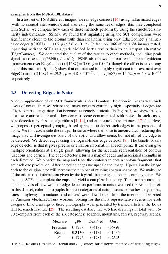
4.3 Detecting Edges in Noise

Another application of our SCF framework is to aid contour detection in images with highlevels of noise. In cases where the image noise is extremely high, especially if edges areof low contrast, edge detection becomes extremely difficult. In Figure 7, we show imagesof a low contrast letter and a low contrast scene contaminated with noise. In such cases,edge detection by classical algorithms [4, 14], and even state-of-the-art ones [17] fail. Here,we propose a perceptual grouping based approach to detect such edges in the presence ofnoise. We first downscale the image. In cases where the noise is uncorrelated, reducing theimage size will average out some of the noise, and allow some, but not all, of the edge tobe detected. We detect edges using the logical-linear edge detector [8]. The benefit of thisedge detector is that it gives precise orientation information at each point. It can even givemultiple orientations at a single point, allowing for the accurate representation of contourjunctions and corners. The edge detector returns a map of edges and associated strengths ineach direction. We binarize the map and trace the contours to obtain contour fragments thatare each one pixel wide. After detecting edges we upscale the image. Up-scaling the imageback to the original size will increase the number of missing contour segments. We make useof the orientation information given by the logical-linear edge detector as our keypoints. Wethen use SCFs to complete the gaps and yield a complete boundary. To perform a more in-depth analysis of how well our edge detection performs in noise, we used the Artist dataset.In this dataset, color photographs from six categories of natural scenes (beaches, city streets,forests, highways, mountains, and offices) were downloaded from the internet and selectedby Amazon MechanicalTurk workers looking for the most representative scenes for eachcategory. Line drawings of these photographs were generated by trained artists at the LotusHill Research Institute [29]. The resulting database had 475 line drawings in total with 76-80 exemplars from each of the six categories: beaches, mountains, forests, highway scenes,

Measure gPb DexiNed OursPrecision 0.1258 0.4189 0.6895

Recall 0.3130 0.1131 0.1636F1 0.1795 0.1781 0.2645

Table 2: Results (Precision, Recall and F1) scores for different methods of detecting edges

10

Noisy Image Low-res Edges DexiNed gPb Ours Ground Truth

Figure 7: Examples of detecting the edges of noisy images. Gaussian noise was added tolow-contrast images of letters (with σ = 39% of the range of the pixel values) and scenes(with σ = 79%). Using SCFs we can make use of the low-resolution edges, by upscalingto the original size and completing the broken contours. The resulting boundary recoversmany more of the edges in the images. The same procedure of downscaling to remove noisedid not improve the performance of the other edge-detection algorithms. See supplementarymaterials for more examples.

city scenes, and office scenes. Images with fire or other potentially upsetting content wereremoved from the experiment (five images total). In Table 2, we compare our method to theDexiNed [17] and gPb [14] algorithms.

5 ConclusionIn this paper, we introduce a modernized SCF algorithm, and demonstrate its power whenintegrated with deep computer vision models. Our improvements include a method for auto-matically finding sources and sinks, so that our SCF algorithm no longer needs to have priorknowledge about the source and sink pairs for computation. In addition, we show that our al-gorithm mechanizes perceptual grouping processes, and mimics results in human perceptionwhen completing broken contour fragments. In addition to a Fokker-Planck equation imple-mentation of the SCF algorithm, we introduce a 4-layer neural network model that computesSCF probability maps using a set of small kernel filters. We show how these implementationscan be substituted into computer vision models that explicitly represent contour information.Specifically, we integrate our SCF blocks with inpainting generative models and models foredge-detection in noisy images. We find that our results outperform the state-of-the-art mod-els with no additional training. Ultimately, our work improves upon the SCF algorithm anddemonstrates how to integrate it in modern computer vision systems.

11

References[1] Irving Biederman and Eric E Cooper. Evidence for complete translational and reflec-

tional invariance in visual object priming. Perception, 20(5):585–593, 1991.

[2] Irving Biederman and Eric E Cooper. Priming contour-deleted images: Evidence forintermediate representations in visual object recognition. Cognitive psychology, 23(3):393–419, 1991.

[3] Charles-Olivier Dufresne Camaro, Morteza Rezanejad, Stavros Tsogkas, Kaleem Sid-diqi, and Sven Dickinson. Appearance shock grammar for fast medial axis extractionfrom real images. In Proceedings of the IEEE/CVF Conference on Computer Visionand Pattern Recognition, pages 14382–14391, 2020.

[4] John Canny. A computational approach to edge detection. IEEE Transactions onpattern analysis and machine intelligence, (6):679–698, 1986.

[5] James Elder and Steven Zucker. The effect of contour closure on the rapid discrimina-tion of two-dimensional shapes. Vision research, 33(7):981–991, 1993.

[6] James H Elder and Steven W Zucker. Computing contour closure. In European Con-ference on Computer Vision, pages 399–412. Springer, 1996.

[7] Qibin Hou, Ming-Ming Cheng, Xiaowei Hu, Ali Borji, Zhuowen Tu, and Philip Torr.Deeply supervised salient object detection with short connections. IEEE TPAMI, 41(4):815–828, 2019. doi: 10.1109/TPAMI.2018.2815688.

[8] Lee A. Iverson and Steven W. Zucker. Logical/linear operators for image curves. IEEETransactions on Pattern Analysis and Machine Intelligence, 17(10):982–996, 1995.

[9] Frank Jäkel, Manish Singh, Felix A Wichmann, and Michael H Herzog. An overviewof quantitative approaches in gestalt perception. Vision research, 126:3–8, 2016.

[10] Kurt Koffka. Perception: an introduction to the gestalt-theorie. Psychological Bulletin,19(10):531, 1922.

[11] Tom Lee, Sanja Fidler, and Sven Dickinson. Learning to combine mid-level cues forobject proposal generation. In Proceedings of the IEEE International Conference onComputer Vision, pages 1680–1688, 2015.

[12] Alex Levinshtein, Cristian Sminchisescu, and Sven Dickinson. Multiscale symmetricpart detection and grouping. International journal of computer vision, 104(2):117–134,2013.

[13] David G. Lowe. Perceptual Organization and Visual Recognition. Kluwer AcademicPublishers, USA, 1985. ISBN 089838172X.

[14] Michael Maire, Pablo Arbeláez, Charless Fowlkes, and Jitendra Malik. Using con-tours to detect and localize junctions in natural images. In 2008 IEEE Conference onComputer Vision and Pattern Recognition, pages 1–8. IEEE, 2008.

[15] Parya Momayyez and Kaleem Siddiqi. 3d stochastic completion fields for fiber trac-tography. In 2009 IEEE Computer Society Conference on Computer Vision and PatternRecognition Workshops, pages 178–185. IEEE, 2009.

12

[16] Kamyar Nazeri, Eric Ng, Tony Joseph, Faisal Z Qureshi, and Mehran Ebrahimi. Edge-connect: Generative image inpainting with adversarial edge learning. arXiv preprintarXiv:1901.00212, 2019.

[17] Xavier Soria Poma, Edgar Riba, and Angel Sappa. Dense extreme inception network:Towards a robust cnn model for edge detection. In Proceedings of the IEEE/CVF WinterConference on Applications of Computer Vision, pages 1923–1932, 2020.

[18] Morteza Rezanejad. Medial measures for recognition, mapping and categorization.McGill University, 2020.

[19] Morteza Rezanejad and Kaleem Siddiqi. View sphere partitioning via flux graphsboosts recognition from sparse views. Frontiers in ICT, 2:24, 2015.

[20] Morteza Rezanejad, Babak Samari, I Rekleitis, Kaleem Siddiqi, and Gregory Dudek.Robust environment mapping using flux skeletons. In 2015 IEEE/RSJ InternationalConference on Intelligent Robots and Systems (IROS), pages 5700–5705. IEEE, 2015.

[21] Morteza Rezanejad, Gabriel Downs, John Wilder, Dirk B Walther, Allan Jepson, SvenDickinson, and Kaleem Siddiqi. Gestalt-based contour weights improve scene cate-gorization by cnns. In Conference on Cognitive Computational Neuroscience (CCN2019), 2019.

[22] Morteza Rezanejad, Gabriel Downs, John Wilder, Dirk B Walther, Allan Jepson, SvenDickinson, and Kaleem Siddiqi. Scene categorization from contours: Medial axis basedsalience measures. In Proceedings of the IEEE/CVF Conference on Computer Visionand Pattern Recognition, pages 4116–4124, 2019.

[23] Sudeep Sarkar and Kim L Boyer. Perceptual organization in computer vision: A reviewand a proposal for a classificatory structure. IEEE Transactions on Systems, Man, andCybernetics, 23(2):382–399, 1993.

[24] Kaleem Siddiqi, Ali Shokoufandeh, Sven J Dickinson, and Steven W Zucker. Shockgraphs and shape matching. International Journal of Computer Vision, 35(1):13–32,1999.

[25] Joan G Snodgrass and Mary Vanderwart. A standardized set of 260 pictures: normsfor name agreement, image agreement, familiarity, and visual complexity. Journal ofexperimental psychology: Human learning and memory, 6(2):174, 1980.

[26] Dor Verbin and Todd Zickler. Field of junctions, 2020.

[27] Johan Wagemans, James H Elder, Michael Kubovy, Stephen E Palmer, Mary A Peter-son, Manish Singh, and Rüdiger von der Heydt. A century of gestalt psychology invisual perception: I. perceptual grouping and figure–ground organization. Psychologi-cal bulletin, 138(6):1172, 2012.

[28] Johan Wagemans, Jacob Feldman, Sergei Gepshtein, Ruth Kimchi, James R Pomer-antz, Peter A van der Helm, and Cees van Leeuwen. A century of gestalt psychology invisual perception: Ii. conceptual and theoretical foundations. Psychological Bulletin,138(6):1218, 2012.

13

[29] Dirk B Walther, Barry Chai, Eamon Caddigan, Diane M Beck, and Li Fei-Fei. Simpleline drawings suffice for functional mri decoding of natural scene categories. Proceed-ings of the National Academy of Sciences, 108(23):9661–9666, 2011.

[30] John Wilder, Morteza Rezanejad, Sven Dickinson, Kaleem Siddiqi, Allan Jepson, andDirk B. Walther. Local contour symmetry facilitates scene categorization. Cog-nition, 182:307 – 317, 2019. ISSN 0010-0277. doi: https://doi.org/10.1016/j.cognition.2018.09.014. URL http://www.sciencedirect.com/science/article/pii/S0010027718302506.

[31] Lance Williams, John Zweck, Tairan Wang, and Karvel Thornber. Computing stochas-tic completion fields in linear-time using a resolution pyramid. Computer Vision andImage Understanding, 76(3):289–297, 1999.

[32] Lance R Williams and David W Jacobs. Local parallel computation of stochastic com-pletion fields. In Proceedings CVPR IEEE Computer Society Conference on ComputerVision and Pattern Recognition, pages 161–168. IEEE, 1996.

[33] Lance R Williams and David W Jacobs. Local parallel computation of stochastic com-pletion fields. Neural computation, 9(4):859–881, 1997.

[34] Lance R Williams and David W Jacobs. Stochastic completion fields: A neural modelof illusory contour shape and salience. Neural computation, 9(4):837–858, 1997.

[35] Andrew P Witkin and Jay M Tenenbaum. On the role of structure in vision. In Humanand machine vision, pages 481–543. Elsevier, 1983.

[36] Wei Xiong, Jiahui Yu, Zhe Lin, Jimei Yang, Xin Lu, Connelly Barnes, and Jiebo Luo.Foreground-aware image inpainting. In Proceedings of the IEEE/CVF Conference onComputer Vision and Pattern Recognition, pages 5840–5848, 2019.

[37] Wei Xiong, Jiahui Yu, Zhe Lin, Jimei Yang, Xin Lu, Connelly Barnes, and Jiebo Luo.Foreground-aware image inpainting. In Proceedings of the IEEE/CVF Conference onComputer Vision and Pattern Recognition (CVPR), June 2019.

[38] Jiahui Yu, Zhe Lin, Jimei Yang, Xiaohui Shen, Xin Lu, and Thomas S. Huang. Genera-tive image inpainting with contextual attention. In Proceedings of the IEEE Conferenceon Computer Vision and Pattern Recognition (CVPR), June 2018.

[39] Jiahui Yu, Zhe Lin, Jimei Yang, Xiaohui Shen, Xin Lu, and Thomas S Huang. Free-form image inpainting with gated convolution. In Proceedings of the IEEE/CVF Inter-national Conference on Computer Vision, pages 4471–4480, 2019.