Continuum QCD2 from a fixed-point lattice action

ANNALS OF PHYSICS 132, 463-481 (1981)

Continuum QCD, from a Fixed-Point Lattice Action*

PAOLO ROSSI’

Center for Theoretical Physics, Laboratory for Nuclear Science and Department of Physics,

Massachusetts Institute of Technology, Cambridge, Massachusetts 02139

Received October 31, 1980

Gauge invariant expectation values for lattice gauge theory with a general local action in two dimensions may be expressed as functions of the single plaquette averages. The value of these averages at the fixed point of the renormalization group can be determined exactly, and the corresponding lattice theory is shown to reproduce the continuum results. The limit N, = 00 is investigated in detail, and fixed point values for all the averages are explicitly determined. Wilson’s action results agree only to first order in weak coupling.

1.

The theory of Yang-Mills fields in two dimensions has been for some time one of the testing grounds of methods to evaluate the properties of nonabelian gauge fields, like the l/N, expansion [I] and the lattice approach [2, 31, and more recently the loop equation of Makeenko and Migdal [4-71.

The only feature that makes this model not completely trivial is the classical long- range static Coulomb potential among charges. In the quantum, gauge invariant formulation of the model this amounts to the existence of nontrivial vacuum expectation values for the Wilson loop operators

W(C) = & Tr (P exp /c A,, dx”) (1.1)

defined on arbitrary closed contours C. W(C) may be in principle explicitly computed, both in the continuum and in the

lattice formulation. This allows us to test another of the current ideas about the properties of gauge theories, i.e., the possibility of recovering the continuum limit through the determination of a fixed point for the renormalization group transformations of the lattice theory.

As we shall show, it is indeed possible to determine explicitly the fixed point lattice

* This work is supported in part through funds provided by the U.S. Department of Energy (DOE) under contract DE-AC02-76ER03069.

t On leave of absence from the Scuola Normale Superiore, Pisa, Italy.

463 0003-4916/81/040463-19$05.00/O

Copyright 0 1981 by Academic Press, Inc. All rights of reproduction in any form reserved.

464 PAOLO ROSS1

theory, to show that it reproduces the continuum behavior and, last but not least, to compare with the known results [3, 81 far away from the fixed point, obtained by assuming the Wilson action

k S( U,) = & Tr[U, + U,+l. e (1.2)

It is amazing to observe that, while the Wilson action results reproduce the continuum in the naive scaling limit, which is, however, specific to the two-dimensional problem because the coupling constant h has the dimensions of an inverse area, they are unrelated to the fixed-point results, which reproduce exactly the continuum without taking any limit. in particular, the third order phase transition found by Gross and Witten [3] in the limit NC = co and their strong coupling results have apparently nothing to do with the behavior of the theory at the fixed point.

This paper is organized as follows: In Section 2 we discuss the properties of lattice gauge theory in two dimensions

when a general local action is assumed, showing that the Wilson loop average may be written as a function of the areas of windows in the loop and of the expectation values of moments of a single plaquette variable and their powers, where all the dependence on the couplings is hidden in the single plaquette averages (“geometrization”).

Tn Section 3, we show how one can determine the fixed-point value of the single plaquette averages by means of a perturbative expansion in the number of loop windows,

In Section 4 we discuss the limit IV, = 00: we write down explicitly the fixed-point values for all the moments, show how to reconstruct the fixed-point action and compare with the continuum and with the Wilson lattice results.

2. LATTICE GAUGE THEORIES IN Two DIMENSIONS

Let us consider a general local lattice action for Yang-Mills theories as a function of the plaquette variable

(2.1)

We are interested in the expectation value of the Wilson loop operator:

QCDa FROM FIXED-POINT LATTICE ACTION 465

where nltc UI is the ordered product of link variables (unitary matrices) along a closed loop C, and DU1 is the group integration.

An extreme simplification in the lattice formulation in two dimensions occurs when we choose the A,, = 0 gauge, corresponding to

U”,@ = 1 (2.4)

and change variables through

u n+O,l = WJJ,,l (2.5)

such that

The partition function J- DUl exp S factorizes, while the Wilson loop operator may be written as a product of plaquette variables involving all the plaquettes enclosed by the loop with an ordering determined by the topology of the loop itself.

It is then obvious that W(C) factorizes into products of factors having the form

.PWewVVf(W) JdWexpS(W) .

(2.7)

Whatever tensor structure may be contained in f( W), these factors may always be reexpressed in terms of invariant tensors and expectation values of the moments of Wand of the products of their powers:

This is a trivial consequence of the invariance of the group measure. All the informa- tion about the explicit dependence of W(C) on the coupling constants him,} may then be reabsorbed in these expectation values.

The only other variables that turn out to be relevant for the complete determination of W(C) are then the “areas” {SK‘) of the loop windows [7], i.e., the number of plaquettes belonging to any sector of the surface spanned by the loop that is completely surrounded by a portion of the loop itself. [A dependence on the relative orientations of the subcontours is also understood.]

We call this result “geometrization” of QCD, and we write it symbolically as

where { W,] is the collection of averages of products of powers of moments of W, and it can also be seen as the collection of all possible loops and products of loops defined on a single plaquette.

We would like to stress the complete generality of the geometrization: no hypothesis

466 PAOLO ROSS1

was made on the form of the action besides the request of locality, and no restrictions on the number of colors IV, were imposed. Further simplifications occurring when N, = cc will be discussed later.

3. DETERMINATION OF THE FIXED POINT

The results of Section 2 allow us to write down the Wilson loop average for an arbitrary loop:

where in principle all the functional dependences may be explicitly determined. However, what we are really interested in is the continuum limit of the theory.

QCD is a simple enough model for the jntegrations we have performed to commute with the naive continuum limit, in which we start from the Wilson action, Eq. (1.2) and because of the physical dimensions of h and {SK} we may operate the scalings

in Eq. (3.1) and take the limit a + 0. It turns out that all singularities cancel out and the naive limit reproduces the continuum result.

However, we cannot hope to be able to mimic this procedure in any model with adimensional couplings, and in general we must address the problem of determining the fixed point of the lattice theory, that is a form of the lattice action such that the theory becomes renormalization group invariant when that action is assumed and, hopefully, the resulting lattice model predicts unambiguously the properties of the corresponding (renormalizable) continuum model.

We should, in principle, find the set of critical couplings (h@~,J)~~r~ corresponding to the fixed-point action. Let us, however, notice that there is a one-to-one correspon- dence between the original parameters of the general local action and the “geometric” parameters W,(h{m,)), and tkanks to the geometrization property we may alter- natively find the set of critical single plaquette expectation values { WIJcrit. We do not expect this determination to lead to a unique solution; rather we expect a residual one-parameter freedom left in the fixed-point theory, amounting to the possibility of an arbitrary change of scale in the dimensions of the lattice and labelled by the “renormalized” coupling A, :

Because of the physical meaning of A, we should then find:

QCDz FROM FIXED-POINT LATTICE ACTION 467

We expect the loop averages W{X,S,]) to coincide in form with the corresponding averages in the continuum theory.

We want to show that a definite, perturbative procedure allowing for the actual determination of the functions (W,} (hR) exists and it can be made unambiguous.

Let us indeed classify the loops according to the number n of their windows (i.e., the number of their self intersections plus 1):

is an n-window loop.

W(S) = W’“‘({W,); s1 )...) S,) (3.5)

Tf we now go back to Eqs. (2.3) and (2.7) it will become apparent that Wcn) depends only on W, (n), the subset of WI defined by xfZI kmK == n. By considering the class of loops Wtn) it is then possible to determine {W JCrit order by order in n simply by writing down the explicit dependence of the loops on (WY’} and (SK> and requiring that the condition Eq. (4.7) be consistently satisfied.

We shall show in Appendix A that this procedure will lead to unique predictions for {W,) if we remove the arbitrariness in the perturbative definition of X, by the “physical” prescription that the expectation values at the fixed point must coincide to first order with the values one obtains by the use of the Wilson action if we make the identification h = X, .

By the way, because of the existence of the naive continuum limit for the action, this is a way to insure us about the identification of h, with the standard continuum coupling.

4. THE N, = co LIMIT

In the large N limit a dramatic simplification occurs due to the property of factorization enjoyed by the expectation values of gauge invariant operators:

(AB) = (A:,(B) + O(N;‘). (4.1)

As a consequence of this property, it is immediate to reexpress ( W,: as a function of the expectation values of the moments of IV:

so that we obtain

W(C) -iyT+ W((U’“,), Is,\). (4.3)

Correspondingly, one may restrict the local action to the class of actions having the form:

(4.4)

468 PAOLO ROSS1

and the fixed point action will correspond to the set {hll)crit or, equivalently, to the set

( w~;$yit) = ( pyWt(jj). (4.5)

The perturbative procedure we have described in Section 3 now becomes much simpler. Tn particular, one may observe that the Ansatz:

( Wn)crit

(( W)crit)n = P’“‘(h) (4.6)

where I’(“‘(;\) is a polynomial of (n - 1)th degree in h, is completely consistent, such that our perturbative method may now be also viewed as a power series expansion in X.

The results of this perturbative analysis (carried on to fourth order in Appendix A) directly confirm order by order a result that could have been guessed by going back- wards from the continuum results (see Appendix B):

where I$’ are the generalized Laguerre polynomials. An explicit power series expansion is

n-1 (n - l)! p’““x) = E, (m $ l)! (n - m - I)!

(-nX)m m! (4.8)

The nontrivial orders of the perturbative expansions in which Eq. (4.7) has been checked and the very structure of the NC = co lattice expectation values of the loop operators leave no reasonable doubt about the correctness of this result, even if a direct proof that the lattice theory corresponding to Eq. (4.7) is renormalization group invariant is by now absent.

We may now address the problem of determining the fixed point couplings (h,}crit. In order to do that we have first to establish the analytic dependence of (w”> on the arbitrary couplings {An). To this purpose we may resort to the loop equation [4], that in the large N limit becomes

(4.9)

The analysis of the loop equation in the single plaquette sector is a generalization of the analysis of Ref. [5].

There is, however, a valuable alternative to this procedure. It is indeed possible to apply saddle point methods to the integral

I d W exp N, ‘? !- Tr( Wn + ~+a) &l %a


extending trivially the technique employed by Gross and Witten [3] to solve the N, --_ cc problem for the Wilson action.

If we introduce a density of eigenvalues p(O) for the eigenvalues eie of W we are led to solving the integral equation

(4.11)

and the “strong coupling” solution to this equation is immediately found by expanding

cot py-) = :! f, (sin ml? cos mg, -- cos mf3 sin my).

The result is

(4.13)

More generally, let us recall that, if we define a generating functional for the moments [5, 61

Q(t) --: ; $- i <w,l;. f”. (4.14) 11-l

Q(t) is an holomorfic function oft when i t I -<, 1 because <n+, 6: I and by considering Q(t) at the boundary of its analyticity domain, that is when t -7 eie, we find that

p(B) e $ Re @(&e) (4.15)

As long as the Fourier series Eq. (4.13) converges between --x and 7~ we are led to the identification

However, even if the convergence properties of the Fourier series are weaker (0, < 7~) it is still true that

s P fil [Re @(eiw)] cot iq) = Im @(eis) I9 < 0, (4.17)

and by comparison with Eq. (4.11) we obtain

(4.18)

470 PAOLO ROSS1

Now, let us remember that the action density, as a function of the eigenvalues of UP has the form

Therefore we obtain from Eq. (4.21)

c

i- $ S(t9) = rm @(eie) e G 4 c (4.20)

and defining s(e) to be the analytic continuation of Im @(eie) on the real axis 0 I> 6, we find

or equivalently

(4.22)

As a matter of fact, we may establish the asymptotic behavior of the coefhcients (w”} for large IZ for the fixed point action, by exploiting the expression of the generalized Laguerre polynomials as confluent hypergeometric functions:

r (1) L,-,(d) = M(I - 12, 2, nX>. (4.23) n

Tt is then possible to show that

L:?,(d) ,z (nh1/2)-3/2w1/2 cos 2~7h1'~ - iv) + O(trz). (4.24)

Notice that the n-3/2 behavior is also found in the weak coupling large n analysis of the moments in the Gross-Witten solution for Wilson’s action [6].

On general grounds, it appears that the Fourier series is not converging fast enough and the strong coupling formula (Eq. (4.16) does not apply for any value of X, so that we have to stick to the genera1 formula Eq. (4.22) in order to reconstruct the action.

As shown in Appendix B, it is possible to perform the summation in Eq. (4.14) when the coefficients are given by Eq. (4.7) and the resulting generating function is defined by

h@(t) - 2 coth-l2@(t) = In t (4.25)

Of course, there exists no solution to the transcendental equation (4.25) in terms of elementary functions, but one may reexpand @ as a power series in h.

QCD2 FROM FIXED-POINT LATTLCE ACTION 471

Tn particular, one may easily check that Q(t) agrees with the corresponding function for the Wilson action only O(h) in weak coupling:

CD(t) = ;= A t(l + f) - 2 (I- -t W). (4.26)

This result might have also been established by considering the known explicit results

[31:

p(B) = & cos i h - sin”:, 8 < 2 sin-l AlI” c Bc (,h < l), (4.27)

(w,, = (1 - ;,, (w") =-= (1 - v (1,2) n-l- p,-2 (1 - 2h) == (1 - A)2 F(2 - n, 2 + n, 2, A), (4.28)

p(O) = & (1 + ; cos e) (A 3 11, (4.29)

(w> = A, (w”j=O, n>l, (4.30)

where P;T,’ are the Jacobi polynomials and F the hypergeometric function. As we mentioned before, the results agree O(h) with the identification X = h, ;

however, the higher orders are definitely different in the two cases. In particular, the third order phase transition for h = 1 completely disappears in the fixed point theory, and the same happens to the whole strong coupling phase of Gross and Witten’s.

The main lesson that one may extract from this analysis is the statement that while the “geometry” of the lattice solution (i.e., the dependence on the areas and on local parameters) is preserved in the renormalization procedure and emerges as a feature of the continuum solution, the dependence on the coupling constant of a particular lattice action, like Wilson’s, does not seem to be directly relevant to the continuum physics, even if that action admits the continuum theory as its naive limit.

APPENDIX A: PERTURBATIVE ANALYSIS

The iterative procedure we have devised in order to determine the fixed-point single plaquette expectation values requires as a preliminary step the determination of the dependence of n-window loops on these expectation values. Since this is going to be the major camputational step in the problem, we want to show how it may be accomplished.

Let us consider an n-window loop (with assigned topology). Jts expectation value is by definition an integral involving a trace of products of Wk’s, where none of the WE’s may appear more than n times.

We can now make use of the fact that the integral is invariant under WE --f VW,V+ for each WE separately, and moreover the action itself is invariant under such transformations. It is then possible to submit a single WE to the transformation and

472 PAOLO ROSS1

integrate over dk’ without affecting the final result. This procedure however will single out the dependence on Wk as a dependence on products of powers of traces of powers of W, while the dependence on all other variables has again the structure of a loop expectation value where all areas now do no longer contain the plaquette asso- ciated with WE .

Moreover, since the overall integration on dWk factorizes the dependence on W, may be further replaced with the dependence on the single plaquette averages (Win’>.

It is now possible to set up recursion relations among loop expectation values corresponding to areas differing by one unit in the form:

W’“‘(S~ )...) S,) = zy w (%), 1 W’“‘(S* )...) s, - l)), (A.11

where 2tn) is a linear combination of the W(“)(& ... S,-,). Knowledge of JdVV ... I+‘+ ... P up to n powers of V (and V+) may be easily

achieved from the knowledge of the generating functional

Z(JJ+) = j- dv eTr(J+Y+JY+)/2 (A.21

that has been evaluated exactly for all U(N) and SU(N) groups [S, 91. The linear first order recursion relations are solved order by order by standard

methods, and the functions W(“)(S 1 ,..., S, , ( W:“‘}) (k < n) are completely determined by the boundary condition that they reduce to Win) when S, = 1, Si = 0 (i < n). The computation may become very cumbersome, but it is always conceptually trival, for high values of n.

Let us now analyze explicitly the first few perturbative terms. The one window problem has already been analyzed for U(N) theories [3] and the known, trivial result is

where

Wfl)(S,) = f (Tr W, e.1 Ws,) = (W(l)(l))sl,

W(l)(l) = 4 (Tr W).

(A.3)

(A.4)

At the two-window level we have to take into account two classes of loops:

Wg’(S, , S,) = -$ (Tr WI **a W,, Tr W, --- Ws,+sI> = W”‘(&) Wk’(O, S,),

(A-6)

where the trivial dependence on S, may be factored out.

QCDa FROM FIXED-POINT LATTICE ACTION 473

If we perform the transformation

(A.7)

and use the U(N) group integral

we find the recursion relations

wp(s 2 Wjf’(S, - 1 j,

(A.9a)

w(2)cs) = N2Wb2’W - @%l) W$‘(l) - Wf’(1) D 2 N2- 1

W$(S -1)3- 2 N2- 1 w3s, - l),

(A.9b)

W?‘(l) z 1 (Tr W2) N ’

WE’(l) 3 -$ ((Tr Wj2).

(A. 10a)

(A.lOb)

It is immediate to find the solution to Eqs. (4.8), (4.9):

w(2)(s ) = N + 1 (

W$%) + NW%) ’ 1

N - 1 (

Wp)(l) - NW$‘(l) )

s2 c 2 2 ISA’ 2 1-N

(A.l’la)

w(2)cs) = N + 1 D 2 2N (

W?(l) + NW%) l+N

1” I N2;l ( W$%)l~~Wi?~l))s’~

(A.1 lb)

At the three-window level there are four different classes of loops relevant to our discussion. Removing a trivial dependence on S, (corresponding to the factor Wr)(S,)) we define:

474 PAOLO ROW

WtA(S, , S,) = & (Tr WI ... W,, WI -1. Ws,+s, Tr WI *.. Ws,+s,), (A.12~)

Wzh(S,, S,) g & (Tr WI *.* Ws3 Tr W, ... Ws,+ Tr W, ... Wsz+s3>. (A.12d)

Again we perform the transformation Eq. (A.6) and find recursion relations, whose solutions are found by imposing Eqs. (A. 11) as boundary conditions when S3 --f 0.

We then obtain:

w%% , S,) = ; Pp-G(&> + K,s3Z,(S,) + 2K,s”Z,(S,)l,

W%S, , S,) = & [Kf%(S,) + K,sZ,(S,) i- 4K,s3Z,(S,)],

&%(s, , S,) = & [K,sZ,(S,) - K:Z,(S,) - 2K,sZ,(S,)],

wm, 3 S,) = 6N2 L K,s"z,W + K,s"-W,) - 4K,s3U&)l,

where

K 1

= 2WM) + NW%(l) + 2NW%(l) + N2Wj%(l) (N + l)(N + 2)

3

K 3

= LW&%(l) - NW$&l) - 2NW%(l) + NZWkh(l) (N - l)(N - 2) 7

K 3

= W$l) - NZW$b(l) 1 - N2

and

Z,(S,) = (N + 2)(NWi?~S,) + W%%)),

Z&T,) = (N - 2)(NW3&) - W$?)(S,)),

Z,(S,) = Wp’(&) - N2 Wt’(&),

Z&Y,) = N(W~‘(S,) - wp(sz)).

Let us recall that

Wgk(l) = $ (Tr W3),

W!,!-(l) = @A(l) z $ (Tr WTr Wz),

W$L(l) = $ ((Tr W)3).

(A.13a)

(A.13b)

(A.13~)

(A.13d)

(A.14a)

(A.14b)

(A.14~)

(A.15a)

(A.15b)

(A.15~)

((A.15d)

(A.16a)

(A.16b)

(A.16c)


The large N limit results may be obtained as limits of the finite N expressions. However, because of factorization there is only one relevant class of loops for each number of windows:

Wcn)(Sl ,..., S,) = & (Tr W, ... WsnWl ... Ws,+snml WI ... ( ) ... ws,+s,~,+...+s,+s,~

(A.17)

and simpler recursion relations may be derived and solved. One then finds:

(A.18a)

W’“‘(S, ) S,) = o+.~l+*s~ [I + s, (g$ - l)], (A.18b)

W’3’(& ) s2 , S,) = (w)~~~+2s~+3s~ [l +sz($$ 1)+s3($$- 1)

+s3(s2+5~3-;)(g3- qp], (A.18~)

W’4’(& ) s, ) s3 ) S,) = (w}s1+2s2+3s3+4s4 [I + s2 (g$ - 1) + s3 (gg - 1)

+s,(s,+;s,-;)(~-- 1)2

- S4(S3 + 4s, - 4) (gg - 1J2

+ s,(s, + 3s3 + 4s4 - 4, ($$ - l)($$ - I)

+s4(-;s4 s3 + s2s3 4- f s32 + ; s,s, + 4s3s4

+ is42 - 6S4 + !$($$ - 1)' + s, ($ - I)].

(A&d)

Let us now undertake the order-by-order reconstruction of the fixed-point expectation values we have described in Section 3. In order to do that, we need to know the single-plaquette averages for the Wilson action up to first order in h. These averages are easily obtained from Eq. (A.2) by observing that

( jfjj ... (A.19)

We are thus led to the following results

W(l)(l) 4 epA12, (A.20a)

595/132/z-16

476 PAOLO ROSS1

v@‘(l)+ 7j--- ( N + 1 pAIN e-~, N - I. eA.‘N

2 1

- W6”‘(1> - (7 N+1 e h.‘N -1 N 1 2N

eA,N 1 e-,l >

(A.21a)

(A.21 b)

W$l> - 1 (N + I)(N + 2) e-3A,N + ItI _ N2) + (N - ‘iN I&/N] e-3~t2,

6 3 (A.22a)

W$L(l) = WL?ll(I) - [ (N + l)(N + ‘4 ep3A,N _ (N - tz(N” - 2, @/N] e-3~~2,

6N (A.22b)

W$Ql> - [ (N + l)(N + 2) +,,N

6N2 2 1 - N” k (N - ;)$ - 2, ,,A:,] e--3~;2. 3 N2 (A.22~)

If we substitute Eqs. (A.20) to (A.22) into Eqs. (A.3), (A.ll), and (A.13) we find:

W’l’(&) ---f e-As+, (A.23)

N - 1 pf,$)(s2) + (AL&!- e-ASz’N - 2 e AS,lhT

1 e-~sz (A.24a)

(A.24b)

e%s2 , S3) + W + 1)W + 2) e-3AS,lN-AS,!N )

6 1 -6N2 (eAS2jN + e-A,c.!,\‘)

+ (N - 1)iN - 2) em,/~+~s,/~

6 1 e-(3/2)ns,-As2, (A.25a)

~%CS2 , S3) - [

0’ + 1)iN + 2) e-“AS,/N-AS,h’ I

6 1 +3N2 (e-As”!N _ ,AWhj

_ iN - l)(N - 2) e3AS,/N+AS,/N (A.25b) 6 1 e-(n!2)As,-As~,

W%(S2 , x3) - [ 0’ + 1W + 2) e-3AS,lN-AS,!N 1 f N’ ie-AS,!N _ e~.s,/~--)

6 6

(A.25~) - (N - l)(N - 2) e3AS,/N+AS,/.V e-(3/2)AS,-AS,,

6 3

Wz%(S, , S3) - [ 1 - N” W + l)(N + 2) e-3AS,/N-AS,/N (e

A&/N + e-A.Sz’N)

6 3

+ (N - l)(N - 2) e3AS,/N+AS,/N

6 I e-(3/2)A+As2. (A.25d)

We may compare these results with the continuum (some of the continuum results for finite N, are presented in Ref. [IO]) and find that there is complete agreement.


In the large N limit we find (either by taking the limit of Eqs. (A.20) to (A.22) or by direct evaluation):

(p,‘; + p-hi? 3 (A.26a)

(:w+, 4 e-*( 1 - X), (A.26b)

.‘; M’” + e-“A/2( 1 - 3x + @2), (A.26~)

/,w4: --f e-2A(I - 6h + 8h2 -- ZjA3) (A.26d)

and Wll’(S,) --f e--(~~2)sI, (A.27a)

W”)(S, , S,) ---f e -(nlz)s,-ns,( * _ AS,), (A.27b)

Wc3)(S, , S2 , S,) --t e -(Ai%)s,-,\sI-(:j,\/z)s,(, _ AS, _ 3XS3 + jj”S,S, + p&2),

(A.27~)

~‘“‘(S, , s, , s, ) ,y,) ---f e~(n’2)S1-~Sp--:~~‘2)S3-2nS4(l _ AS2 - 3j& -+ h”S,S, + $x”&z

- 6X& + 3X’S,& + 8h2S& -+ 8X2Sa2 - h”S,S,S,

- p”s,s,2 -- 4h3S3S43 - $w32s4 - $PS 3 4 (A.27)

These results match exactly with the results one would have obtained by performing the direct integration in the continuum theory, as we shall show in Appendix B.

For the sake of comparison, let us give explicit expressions for the Wilson’s action moments:

x .,,M’: =z 1 - - 2’

;&y E (1 - A)%,

,!W3’i =: (I - h)2( 1 - %,A), (A.28)

,‘w4;> = ( I - h)2( I - 6h + 7h2).

There is definitely no agreement besides the first order agreement we have imposed.

FIG. I. Expectation values of (1 /NJ Tr W for the fixed point action (continuous line) and for Wilson’s action (dashed line) in the limit NC 2 a’.

478 PAOLO ROSS1

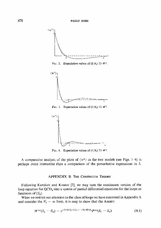
FIG. 2. Expectation values of (l/N,) Tr IV”.

FIG. 3. Expectation values of (l/N,) Tr PP.

FIG. 4. Expectation values of (l/N,) Tr W4.

A comparative analysis of the plots of (IV”) in the two models (see Figs. l-4) is perhaps more instructive than a comparison of the perturbative expressions in X.

APPENDIX B: THE CONTINUUM THEORY

Following Kazakov and Kostov [7], we may turn the continuum version of the loop equation for QCD, into a system of partial differential equations for the loops as functions of {S,}.

When we restrict our attention to the class of loops we have examined in Appendix A and consider the N, = cc limit, it is easy to show that the Ansatz:

wys . . . s ) 1%

= f-(~/2)s,-As,-...-(n/z)As~~(~)(s ... s 1 n

) @.I)


(where I’(“) is a polynomial of (n - 1)th degree in A&) is consistent with the equations, that in turn may be written in the form:

= xP”“ys, , s, ,.... s, + ... + As,) P(“--“%$$+l )...) S,,). 03.2)

It is possible to show that the boundary condition W’“)(O) = I leads to the solutions:

P(l’(S,) = 1)

P’2’(S, ) S,) = 1 - AS, )

P3’(S, ) s, , S,) = 1 ~ AS, - 3hS, + h?!g, + #h?!2,2,

P4’(Sl , S, , S3 , S,) = 1 ~ /\S, - 3hS, + x2S2S, + $X2S32 - 6AS, + 3h2SzS,

-I- 8X”S,S* + ws,2 - P&s,s, - gw,s,2 - 4X3&S,”

--ox3s,?Y4 - 93&3. 03.3)

Successive substitutions allow one to extract from Eqs. (B.2) the equation:

c

d P(IL) = X[P”‘(S,) P”yS,s, ... s,-, + S,) -_

%S,

+ 2P’ys,-, ) S,) P’“-y&s2 )...) Se + &_I + S,)

- t -.. + (n -- I) P’l’(S, + ... + S ) P(11-1)(S2 ,..., S,)] n (B.4)

and in the special case when Si = 0 i < n Eq. (B.4) reduces to

ii n-1 -____

w&) fJ’“)(hS,) = c mP’““‘(XS,) P(‘L-nf)(&J.

I%=1

We may turn Eq. (B.5) into the equation

(B.5)

by defining a generating function

Q&Is, t) = f P’“‘(hS) t” 7kl

(B.7)

satisfying the boundary conditions

$(t = 0) = 0 $qhS = 0) = & . (B.8)

One may apply the standard methods for quasilinear first order partial differential

480 PAOLO ROW

equations and find that the solution to Eq. (B.6) with boundary conditions (B.8) is

___ exp AS* = t. 1+4J

We have also found that the solution may be expressed in the form

(B.lO)

where Li‘?) are the generalized Laguerre polynomials. This result has been independent- ly recovered by Giles [l 11.

The structure of the lattice loop expectation values IVn) in the limiting case when & = 0, i < n and S, = 1 makes it apparent that the choice, if any, turning the lattice solution into the continuum solution is

The consistency of this choice has been checked perturbatively in Appendix A. Let us notice that the generating function of the (w”>, defined in Eq. (4. I7), is now

related to the function # defined in Eq. (B.7) by:

G(t) = 4 + #(A, te-A/2).

It is then immediate to obtain @ in the form

0-s Q + L exp h@ 1:: exp[X@ - 2 cothp12@n] / t (B.12)

2

(B.ll)

that leads to Eq. (4.25).

ACKNOWLEDGMENTS

I would like to thank Roscoe Giles, Richard Brower, and Chung-I Tan for helpful conversations and suggestions.

REFERENCES

1. G. T’HOOFT, Nucl. Phys. 872 (1974), 461; 75 (1974), 461. 2. K. WILSON, Phys. Rev. D 10 (1974), 2445. 3. D. J. GROSS ANJJ E. WITTEN, Phys. Rev. D 21 (1980), 446. 4. Y. M. MAKEENKO AND A. A. MIGDAL, Phys. Len. B88 (1979), 135. 5. G. PAFFUTI AND P. Ross, Phys. Lett. B 92 (1980), 321. 6. D. FRIEDAN, “Some Nonabelian Toy Models in the Large N Limit,” Berkeley preprint (1980).

QCD? FROM FIXED-POINT LATTICE ACTION 481

7. V. A. KAZAKOV AND I. K. KOSTOV, “Nonlinear Strings in Two-dimensional U(m) GaugeTheory,” Landau Institute preprint 1980-9.

8. R. BROWER, P. ROSSI, AND C.-I. TAN, Phys. Rev. D 23 (1981), 942. 9. R. BROWER, P. Rossr, AND C.-I. TAN, Brown HET-445 preprint.

10. V. A. KAZAKOV, “Wilson Loop Average for an Arbitrary Contour in 2-Dim U(N)GaugeTheory,” Landau Institute preprint 1980-16.

Il. R. GILES, private communication.

Documents

Continuum QCD2 from a fixed-point lattice action