Continuous Time Analysis of Momentum Methods

Journal of Machine Learning Research 22 (2021) 1-40 Submitted 6/19; Revised 9/20; Published 1/21

Continuous Time Analysis of Momentum Methods

Nikola B. Kovachki [email protected] and Mathematical SciencesCalifornia Institute of TechnologyPasadena, CA 91125, USA

Andrew M. Stuart [email protected]

Computing and Mathematical Sciences

California Institute of Technology

Pasadena, CA 91125, USA

Editor: Suvrit Sra

Abstract

Gradient descent-based optimization methods underpin the parameter training of neuralnetworks, and hence comprise a significant component in the impressive test results foundin a number of applications. Introducing stochasticity is key to their success in practicalproblems, and there is some understanding of the role of stochastic gradient descent in thiscontext. Momentum modifications of gradient descent such as Polyak’s Heavy Ball method(HB) and Nesterov’s method of accelerated gradients (NAG), are also widely adopted. Inthis work our focus is on understanding the role of momentum in the training of neuralnetworks, concentrating on the common situation in which the momentum contribution isfixed at each step of the algorithm. To expose the ideas simply we work in the deterministicsetting.

Our approach is to derive continuous time approximations of the discrete algorithms;these continuous time approximations provide insights into the mechanisms at play withinthe discrete algorithms. We prove three such approximations. Firstly we show that stan-dard implementations of fixed momentum methods approximate a time-rescaled gradientdescent flow, asymptotically as the learning rate shrinks to zero; this result does not dis-tinguish momentum methods from pure gradient descent, in the limit of vanishing learningrate. We then proceed to prove two results aimed at understanding the observed practicaladvantages of fixed momentum methods over gradient descent, when implemented in thenon-asymptotic regime with fixed small, but non-zero, learning rate. We achieve this byproving approximations to continuous time limits in which the small but fixed learning rateappears as a parameter; this is known as the method of modified equations in the numericalanalysis literature, recently rediscovered as the high resolution ODE approximation in themachine learning context. In our second result we show that the momentum method is ap-proximated by a continuous time gradient flow, with an additional momentum-dependentsecond order time-derivative correction, proportional to the learning rate; this may be usedto explain the stabilizing effect of momentum algorithms in their transient phase. Fur-thermore in a third result we show that the momentum methods admit an exponentiallyattractive invariant manifold on which the dynamics reduces, approximately, to a gradientflow with respect to a modified loss function, equal to the original loss function plus a smallperturbation proportional to the learning rate; this small correction provides convexifica-tion of the loss function and encodes additional robustness present in momentum methods,beyond the transient phase.

c©2021 Nikola B. Kovachki and Andrew M. Stuart.

License: CC-BY 4.0, see https://creativecommons.org/licenses/by/4.0/. Attribution requirements are providedat http://jmlr.org/papers/v22/19-466.html.

https://creativecommons.org/licenses/by/4.0/

http://jmlr.org/papers/v22/19-466.html

Kovachki and Stuart

Keywords: Optimization, Machine Learning, Deep Learning, Gradient Flows, Momen-tum Methods, Modified Equation, Invariant Manifold

1. Introduction

1.1 Background and Literature Review

At the core of many machine learning tasks is solution of the optimization problem

arg minu∈Rd

Φ(u) (1)

where Φ : Rd → R is an objective (or loss) function that is, in general, non-convex and differ-entiable. Finding global minima of such objective functions is an important and challengingtask with a long history, one in which the use of stochasticity has played a prominent rolefor many decades, with papers in the early development of machine learning Geman andGeman (1987); Styblinski and Tang (1990), together with concomitant theoretical analysesfor both discrete Bertsimas et al. (1993) and continuous problems Kushner (1987); Kushnerand Clark (2012). Recent successes in the training of deep neural networks have built onthis older work, leveraging the enormous computer power now available, together with em-pirical experience about good design choices for the architecture of the networks; reviewsmay be found in Goodfellow et al. (2016); LeCun et al. (2015). Gradient descent playsa prominent conceptual role in many algorithms, following from the observation that theequation

du

dt= −∇Φ(u) (2)

will decrease Φ along trajectories. The most widely adopted methods use stochastic gradientdecent (SGD), a concept introduced in Robbins and Monro (1951); the basic idea is to usegradient decent steps based on a noisy approximation to the gradient of Φ. Building on deepwork in the convex optimization literature, momentum-based modifications to stochasticgradient decent have also become widely used in optimization. Most notable amongst thesemomentum-based methods are the Heavy Ball Method (HB), due to Polyak (1964), andNesterov’s method of accelerated gradients (NAG) Nesterov (1983). To the best of ourknowledge, the first application of HB to neural network training appears in Rumelhartet al. (1986). More recent work, such as Sutskever et al. (2013), has even argued for theindispensability of such momentum based methods for the field of deep learning.

From these two basic variants on gradient decent, there have come a plethora of adap-tive methods, incorporating momentum-like ideas, such as Adam Kingma and Ba (2014),Adagrad Duchi et al. (2011), and RMSProp Tieleman and Hinton (2012). There is no con-sensus on which method performs best and results vary based on application. The recentwork of Wilson et al. (2017) argues that the rudimentary, non-adaptive schemes SGD, HB,and NAG result in solutions with the greatest generalization performance for supervisedlearning applications with deep neural network models.

There is a natural physical analogy for momentum methods, namely that they relate toa damped second order Hamiltonian dynamic with potential Φ:

md2u

dt2+ γ(t)

du

dt+∇Φ(u) = 0. (3)

2


This perspective goes back to Polyak’s original work Polyak (1964, 1987) and was furtherexpanded on in Qian (1999), although no proof was given. For NAG, the work of Su et al.(2014) proves that the method approximates a damped Hamiltonian system of precisely thisform, with a time-dependent damping coefficient. The analysis in Su et al. (2014) holdswhen the momentum factor is chosen according to the rule

λ = λn =n

n+ 3, (4)

where n is the iteration count; this choice was proposed in the original work of Nesterov(1983) and results in a choice of λ which is asymptotic to 1. In the setting where Φ isµ-strongly convex, it is proposed in Nesterov (2014) that the momentum factor is fixed andchosen close to 1; specifically it is proposed that

λ =1−√µh

1 +√µh

(5)

where h > 0 is the time-step (learning rate). In Wilson et al. (2016), a limiting equationfor both HB and NAG of the form

u+ 2√µu+∇Φ(u) = 0

is derived under the assumption that λ is fixed with respect to iteration number n, anddependent on the time-step h as specified in (5); convergence is obtained to order O(h1/2).Using insight from this limiting equation it is possible to choose the optimal value of µ tomaximize the convergence rate in the neighborhood of a locally strongly convex objectivefunction. Further related work is developed in Shi et al. (2018) where separate limitingequations for HB and NAG are derived both in the cases of λ given by (4) and (5), obtainingconvergence to order O(h3/2). Much work has also gone into analyzing these methods in thediscrete setting, without appeal to the continuous time limits, see Hu and Lessard (2017);Lessard et al. (2016), as well as in the stochastic setting, establishing how the effect on thegeneralization error, for example, Gadat et al. (2018); Loizou and Richtarik (2017); Yanget al. (2016). In this paper, however, our focus is on the use of continuous time limits as amethodology to explain optimization algorithms.

In many machine learning applications, especially for deep learning, NAG and HB areoften used with a constant momentum factor λ that is chosen independently of the iterationcount n (contrary to (4)) and independently of the learning rate h (contrary to (5)). Infact, popular books on the subject such as Goodfellow et al. (2016) introduce the methodsin this way, and popular articles, such as He et al. (2016) to name one of many, simplystate the value of the constant momentum factor used in their experiments. Widely useddeep learning libraries such as Tensorflow Abadi et al. (2015) and PyTorch Paszke et al.(2017) implement the methods with a fixed choice of momentum factor. Momentum basedmethods used in this way, with fixed momentum, have not been carefully analyzed. Wewill undertake such an analysis, using ideas from numerical analysis, and in particularthe concept of modified equations Griffiths and Sanz-Serna (1986); Chartier et al. (2007)and from the theory of attractive invariant manifolds Hirsch et al. (2006); Wiggins (2013);both ideas are explained in the text Stuart and Humphries (1998). It is noteworthy that

3

Kovachki and Stuart

the high resolution ODE approximation described in Shi et al. (2018) may be viewed as arediscovery of the method of modified equations. We emphasize the fact that our work isnot at odds with any previous analyses of these methods, rather, we consider a setting whichis widely adopted in deep learning applications and has not been subjected to continuoustime analysis to date.

1.2 Our Contribution

We study momentum-based optimization algorithms for the minimization task (1), withlearning rate independent momentum, fixed at every iteration step, focusing on determin-istic methods for clarity of exposition. Our approach is to derive continuous time approxi-mations of the discrete algorithms; these continuous time approximations provide insightsinto the mechanisms at play within the discrete algorithms. We prove three such approxi-mations. The first shows that the asymptotic limit of the momentum methods, as learningrate approaches zero, is simply a rescaled gradient flow (2). The second two approxima-tions include small perturbations to the rescaled gradient flow, on the order of the learningrate, and give insight into the behavior of momentum methods when implemented withmomentum and fixed learning rate. Through these approximation theorems, and accompa-nying numerical experiments, we make the following contributions to the understanding ofmomentum methods as often implemented within machine learning:

• We show that momentum-based methods with a fixed momentum factor, satisfy, inthe continuous-time limit obtained by sending the learning rate to zero, a rescaledversion of the gradient flow equation (2).

• We show that such methods also approximate a damped Hamiltonian system of theform (3), with small mass m (on the order of the learning rate) and constant dampingγ(t) = γ; this approximation has the same order of accuracy as the approximation ofthe rescaled equation (2) but provides a better qualitative understanding of the fixedlearning rate momentum algorithm in its transient phase.

• We also show that, for the approximate Hamiltonian system, the dynamics admit anexponentially attractive invariant manifold, locally representable as a graph mappingco-ordinates to their velocities. The map generating this graph describes a gradientflow in a potential which is a small (on the order of the learning rate) perturbation of Φ– see (21); the correction to the potential is convexifying, does not change the globalminimum, and provides insight into the fixed learning rate momentum algorithmbeyond its initial transient phase.

• We provide numerical experiments which illustrate the foregoing considerations, forsimple linear test problems, and for the MNIST digit classification problem; in thelatter case we consider SGD and thereby demonstrate that the conclusions of ourtheory have relevance for understanding the stochastic setting as well.

Taken together our results are interesting because they demonstrate that the popularbelief that (fixed) momentum methods resemble the dynamics induced by (3) is misleading.Whilst it is true, the mass in the approximating equation is small and as a consequence

4


understanding the dynamics as gradient flows (2), with modified potential, is more instruc-tive. In fact, in the first application of HB to neural networks described in Rumelhartet al. (1986), the authors state that “[their] experience has been that [one] get[s] the samesolutions by setting [the momentum factor to zero] and reducing the size of [the learningrate].” However our theorems should not be understood to imply that there is no practicaldifference between momentum methods (with fixed learning rate) and SGD. There is indeeda practical difference as has been demonstrated in numerous papers throughout the machinelearning literature, and our experiments in Section 5 further confirm this. We show thatwhile these methods have the same transient dynamics, they are approximated differently.Our results demonstrate that, although momentum methods behave like a gradient descentalgorithm, asymptotically, this algorithm has a modified potential. Furthermore, althoughthis modified potential (20) is on the order of the learning rate, the fact that the learningrate is often chosen as large as possible, constrained by numerical stability, means that thecorrection to the potential may be significant. Our results may be interpreted as indicatingthat the practical success of momentum methods stems from the fact that they provide amore stable discretization to (2) than the forward Euler method employed in SGD. Thedamped Hamiltonian dynamic (11), as well the modified potential, give insight into howthis manifests. Our work gives further theoretical justification for the exploration of the useof different numerical integrators for the purposes of optimization such as those performedin Scieur et al. (2017); Betancourt et al. (2018); Zhang et al. (2018).

While our analysis is confined to the non-stochastic case to simplify the exposition, theresults will, with some care, extend to the stochastic setting using ideas from averaging andhomogenization Pavliotis and Stuart (2008) as well as continuum analyses of SGD as in Liet al. (2017); Feng et al. (2018); indeed, in the stochastic setting, sharp uniform in time errorestimates are to be expected for empirical averages Mattingly et al. (2010); Dieuleveut et al.(2017). To demonstrate that our analysis is indeed relevant in the stochastic setting, wetrain a deep autoencoder with mini-batching (stochastic) and verify that our convergenceresults still hold. The details of this experiment are given in section 5. Furthermore wealso confine our analysis to fixed learning rate, and impose global bounds on the relevantderivatives of Φ; this further simplifies the exposition of the key ideas, but is not essentialto them; with considerably more analysis the ideas exposed in this paper will transfer toadaptive time-stepping methods and much less restrictive classes of Φ.

The paper is organized as follows. Section 2 introduces the optimization proceduresand states the convergence result to a rescaled gradient flow. In section 3 we derive themodified, second-order equation and state convergence of the schemes to this equation.Section 4 asserts the existence of an attractive invariant manifold, demonstrating that itresults in a gradient flow with respect to a small perturbation of Φ. In section 5, we traina deep autoencoder, showing that our results hold in a stochastic setting with Assumption1 violated. We conclude in section 6. All proofs of theorems are given in the appendices sothat the ideas of the theorems can be presented clearly within the main body of the text.

1.3 Notation

We use | · | to denote the Euclidean norm on Rd. We define f : Rd → Rd by f(u) := −∇Φ(u)for any u ∈ Rd. Given parameter λ ∈ [0, 1) we define λ := (1− λ)−1.

5

Kovachki and Stuart

For two Banach spaces A,B, and A0 a subset in A, we denote by Ck(A0;B) the set ofk-times continuously differentiable functions with domain A0 and range B. For a functionu ∈ Ck(A0;B), we let Dju denote its j-th (total) Frechet derivative for j = 1, . . . , k. For

a function u ∈ Ck([0,∞),Rd), we denote its derivatives by dudt ,

d2udt2, etc. or equivalently by

u, u, etc.

To simplify our proofs, we make the following assumption about the objective function.

Assumption 1 Suppose Φ ∈ C3(Rd;R) with uniformly bounded derivatives. Namely, thereexist constants B0, B1, B2 > 0 such that

‖Dj−1f‖ = ‖DjΦ‖ ≤ Bj−1

for j = 1, 2, 3 where ‖ · ‖ denotes any appropriate operator norm.

We again stress that this assumption is not key to developing the ideas in this work,but is rather a simplification used to make our results global. Without Assumption 1, andno further assumption on Φ such as convexity, one could only hope to give local resultsi.e. in the neighborhood of a critical point of Φ. Such analysis could indeed be carried out(see for example Carr (2012)), but we choose not to do so here for the sake of clarity ofexposition. In section 5, we give a practical example where this assumption is violated andyet the behavior is as predicted by our theory.

Finally we observe that the nomenclature “learning rate” is now prevalent in machinelearning, and so we use it in this paper; it refers to the object commonly referred to as“time-step” in the field of numerical analysis.

2. Momentum Methods and Convergence to Gradient Flow

In subsection 2.1 we state Theorem 2 concerning the convergence of a class of momentummethods to a rescaled gradient flow. Subsection 2.2 demonstrates that the HB and NAGmethods are special cases of our general class of momentum methods, and gives intuitionfor proof of Theorem 2; the proof itself is given in Appendix A. Subsection 2.3 contains anumerical illustration of Theorem 2.

2.1 Main Result

The standard Euler discretization of (2) gives the discrete time optimization scheme

un+1 = un + hf(un), n = 0, 1, 2, . . . . (6)

Implementation of this scheme requires an initial guess u0 ∈ Rd. For simplicity we considera fixed learning rate h > 0. Equation (2) has a unique solution u ∈ C3([0,∞);Rd) underAssumption 1 and for un = u(nh)

sup0≤nh≤T

|un − un| ≤ C(T )h;

see Stuart and Humphries (1998), for example.

6


In this section we consider a general class of momentum methods for the minimizationtask (1) which can be written in the form, for some a ≥ 0 and λ ∈ (0, 1),

un+1 = un + λ(un − un−1) + hf(un + a(un − un−1)), n = 0, 1, 2, . . . ,

u1 = u0 + hf(u0) .(7)

Again, implementation of this scheme requires an an initial guess u0 ∈ Rd. The parameterchoice a = 0 gives HB and a = λ gives NAG. In Appendix A we prove the following:

Theorem 2 Suppose Assumption 1 holds and let u ∈ C3([0,∞);Rd) be the solution to

du

dt= −(1− λ)−1∇Φ(u)

u(0) = u0

(8)

with λ ∈ (0, 1). For n = 0, 1, 2, . . . let un be the sequence given by (7) and define un := u(nh).Then for any T ≥ 0, there is a constant C = C(T ) > 0 such that

sup0≤nh≤T

|un − un| ≤ Ch.

Note that (8) is simply a sped-up version of (2): if v solves (2) and w solves (8) thenv(t) = w((1 − λ)t) for any t ∈ [0,∞). This demonstrates that introduction of momentumin the form used within both HB and NAG results in numerical methods that do not differsubstantially from gradient descent.

2.2 Link to HB and NAG

The HB method is usually written as a two-step scheme taking the form (Sutskever et al.(2013))

vn+1 = λvn + hf(un)

un+1 = un + vn+1

with v0 = 0, λ ∈ (0, 1) the momentum factor, and h > 0 the learning rate. We can re-writethis update as

un+1 = un + λvn + hf(un)

= un + λ(un − un−1) + hf(un)

hence the method reads

un+1 = un + λ(un − un−1) + hf(un)

u1 = u0 + hf(u0).(9)

Similarly NAG is usually written as (Sutskever et al. (2013))

vn+1 = λvn + hf(un + λvn)

un+1 = un + vn+1

7

Kovachki and Stuart

with v0 = 0. Define wn := un + λvn then

wn+1 = un+1 + λvn+1

= un+1 + λ(un+1 − un)

and

un+1 = un + λvn + hf(un + λvn)

= un + (wn − un) + hf(wn)

= wn + hf(wn).

Hence the method may be written as

un+1 = un + λ(un − un−1) + hf(un + λ(un − un−1))

u1 = u0 + hf(u0).(10)

It is clear that (9) and (10) are special cases of (7) with a = 0 giving HB and a = λgiving NAG. To intuitively understand Theorem 2, re-write (8) as

du

dt− λdu

dt= f(u).

If we discretize the du/dt term using forward differences and the −λdu/dt term usingbackward differences, we obtain

u(t+ h)− u(t)

h− λu(t)− u(t− h)

h≈ f(u(t)) ≈ f

(u(t) + ha

u(t)− u(t− h)

h

)with the second approximate equality coming from the Taylor expansion of f . This can berearranged as

u(t+ h) ≈ u(t) + λ(u(t)− u(t− h)) + hf(u(t) + a(u(t)− u(t− h)))

which has the form of (7) with the identification un ≈ u(nh).

2.3 Numerical Illustration

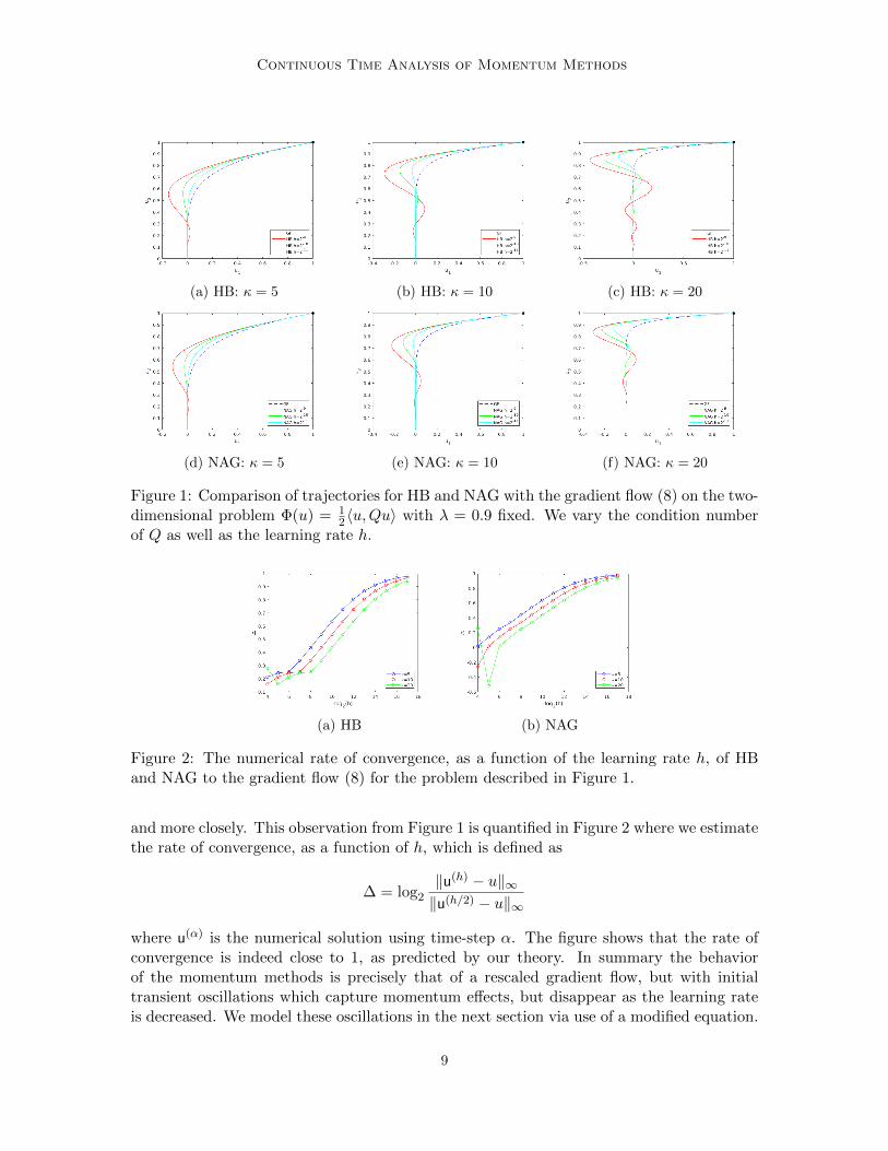
Figure 1 compares trajectories of the momentum numerical method (7) with the rescaledgradient flow (8), for the two-dimensional problem Φ(u) = 1

2〈u,Qu〉. We pick Q to bepositive-definite so that the minimum is achieved at the point (0, 0)T and make it diagonalso that we can easily control its condition number. In particular, the condition number ofQ is given as

κ =max{Q11, Q22}min{Q11, Q22}

.

We see that, as the condition number is increased, both HB and NAG exhibit more pro-nounced transient oscillations and are thus further away from the trajectory of (8), however,as the learning rate h is decreased, the oscillations dampen and the trajectories match more

8


(a) HB: κ = 5 (b) HB: κ = 10 (c) HB: κ = 20

(d) NAG: κ = 5 (e) NAG: κ = 10 (f) NAG: κ = 20

Figure 1: Comparison of trajectories for HB and NAG with the gradient flow (8) on the two-dimensional problem Φ(u) = 1

2〈u,Qu〉 with λ = 0.9 fixed. We vary the condition numberof Q as well as the learning rate h.

(a) HB (b) NAG

Figure 2: The numerical rate of convergence, as a function of the learning rate h, of HBand NAG to the gradient flow (8) for the problem described in Figure 1.

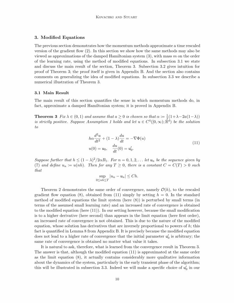
and more closely. This observation from Figure 1 is quantified in Figure 2 where we estimatethe rate of convergence, as a function of h, which is defined as

∆ = log2

‖u(h) − u‖∞‖u(h/2) − u‖∞

where u(α) is the numerical solution using time-step α. The figure shows that the rate ofconvergence is indeed close to 1, as predicted by our theory. In summary the behaviorof the momentum methods is precisely that of a rescaled gradient flow, but with initialtransient oscillations which capture momentum effects, but disappear as the learning rateis decreased. We model these oscillations in the next section via use of a modified equation.

9

Kovachki and Stuart

3. Modified Equations

The previous section demonstrates how the momentum methods approximate a time rescaledversion of the gradient flow (2). In this section we show how the same methods may also beviewed as approximations of the damped Hamiltonian system (3), with mass m on the orderof the learning rate, using the method of modified equations. In subsection 3.1 we stateand discuss the main result of the section, Theorem 3. Subsection 3.2 gives intuition forproof of Theorem 3; the proof itself is given in Appendix B. And the section also containscomments on generalizing the idea of modified equations. In subsection 3.3 we describe anumerical illustration of Theorem 3.

3.1 Main Result

The main result of this section quantifies the sense in which momentum methods do, infact, approximate a damped Hamiltonian system; it is proved in Appendix B.

Theorem 3 Fix λ ∈ (0, 1) and assume that a ≥ 0 is chosen so that α := 12(1+λ−2a(1−λ))

is strictly positive. Suppose Assumption 1 holds and let u ∈ C4([0,∞);Rd) be the solutionto

hαd2u

dt2+ (1− λ)

du

dt= −∇Φ(u)

u(0) = u0,du

dt(0) = u′0.

(11)

Suppose further that h ≤ (1− λ)2/2αB1. For n = 0, 1, 2, . . . let un be the sequence given by(7) and define un := u(nh). Then for any T ≥ 0, there is a constant C = C(T ) > 0 suchthat

sup0≤nh≤T

|un − un| ≤ Ch.

Theorem 2 demonstrates the same order of convergence, namely O(h), to the rescaledgradient flow equation (8), obtained from (11) simply by setting h = 0. In the standardmethod of modified equations the limit system (here (8)) is perturbed by small terms (interms of the assumed small learning rate) and an increased rate of convergence is obtainedto the modified equation (here (11)). In our setting however, because the small modificationis to a higher derivative (here second) than appears in the limit equation (here first order),an increased rate of convergence is not obtained. This is due to the nature of the modifiedequation, whose solution has derivatives that are inversely proportional to powers of h; thisfact is quantified in Lemma 8 from Appendix B. It is precisely because the modified equationdoes not lead to a higher rate of convergence that the initial parameter u′0 is arbitrary; thesame rate of convergence is obtained no matter what value it takes.

It is natural to ask, therefore, what is learned from the convergence result in Theorem 3.The answer is that, although the modified equation (11) is approximated at the same orderas the limit equation (8), it actually contains considerably more qualitative informationabout the dynamics of the system, particularly in the early transient phase of the algorithm;this will be illustrated in subsection 3.3. Indeed we will make a specific choice of u′0 in our

10


numerical experiments, namely

du

dt(0) =

1− 2α

2α− λ+ 1f(u0), (12)

to better match the transient dynamics.

3.2 Intuition and Wider Context

3.2.1 Idea Behind The Modified Equations

In this subsection, we show that the scheme (7) exhibits momentum, in the sense of ap-proximating a momentum equation, but the size of the momentum term is on the order ofthe step size h. To see this intuitively, we add and subtract un−un−1 to the right hand sizeof (7) then we can rearrange it to obtain

hun+1 − 2un + un−1

h2+ (1− λ)

un − un−1

h= f(un + a(un − un−1)).

This can be seen as a second order central difference and first order backward differencediscretization of the momentum equation

hd2u

dt2+ (1− λ)

du

dt= f(u)

noting that the second derivative term has size of order h.

3.2.2 Higher Order Modified Equations For HB

We will now show that, for HB, we may derive higher order modified equations that areconsistent with (9). Taking the limit of these equations yields an operator that agrees withwith our intuition for discretizing (8). To this end, suppose Φ ∈ C∞b (Rd,R) and considerthe ODE(s),

p∑k=1

hk−1(1 + (−1)kλ)

k!

dku

dtk= f(u) (13)

noting that p = 1 gives (8) and p = 2 gives (11). Let u ∈ C∞([0,∞),Rd) be the solution to

(13) and define un := u(nh), u(k)n := dku

dtk(nh) for n = 0, 1, 2, . . . and k = 1, 2, . . . , p. Taylor

expanding yields

un±1 = un +

p∑k=1

(±1)khk

k!u(k)n + hp+1I±n

where

I±n =(±1)p+1

p!

∫ 1

0(1− s)pd

p+1u

dtp+1((n± s)h)ds.

11

Kovachki and Stuart

Then

un+1 − un − λ(un − un−1) =

p∑k=1

hk

k!u(k)n + λ

p∑k=1

(−1)khk

k!u(k)n + hp+1(I+

n − λI−n )

= h

p∑k=1

hk−1(1 + (−1)kλ)

k!u(k)n + hp+1(I+

n − λI−n )

= hf(un) + hp+1(I+n − λI−n )

showing consistency to order p+ 1. As is the case with (11) however, the I±n terms will beinversely proportional to powers of h hence global accuracy will not improve.

We now study the differential operator on the l.h.s. of (13) as p → ∞. Define thesequence of differential operators Tp : C∞([0,∞),Rd)→ C∞([0,∞),Rd) by

Tpu =

p∑k=1

hk−1(1 + (−1)kλ)

k!

dku

dtk, ∀u ∈ C∞([0,∞),Rd).

Taking the Fourier transform yields

F(Tpu)(ω) =

p∑k=1

hk−1(1 + (−1)kλ)(iω)k

k!F(u)(ω)

where i =√−1 denotes the imaginary unit. Suppose there is a limiting operator Tp → T

as p→∞ then taking the limit yields

F(Tu)(ω) =1

h(eihω + λe−ihω − λ− 1)F(u)(ω).

Taking the inverse transform and using the convolution theorem, we obtain

(Tu)(t) =1

hF−1(eihω + λe−ihω − λ− 1)(t) ∗ u(t)

=1

h(−(1 + λ)δ(t) + λδ(t+ h) + δ(t− h)) ∗ u(t)

=1

h

∫ ∞−∞

(−(1 + λ)δ(t− τ) + λδ(t− τ + h) + δ(t− τ − h))u(τ) dτ

=1

h(−(1 + λ)u(t) + λu(t− h) + u(t+ h))

=u(t+ h)− u(t)

h− λ

(u(t)− u(t− h)

h

)where δ(·) denotes the Dirac-delta distribution and we abuse notation by writing its actionas an integral. The above calculation does not prove convergence of Tp to T , but simplyconfirms our intuition that (9) is a forward and backward discretization of (8).

12


(a) HB: κ = 5 (b) HB: κ = 10 (c) HB: κ = 20

(d) NAG: κ = 5 (e) NAG: κ = 10 (f) NAG: κ = 20

Figure 3: Comparison of trajectories for HB and NAG with the Hamiltonian dynamic (11)on the two-dimensional problem Φ(u) = 1

2〈u,Qu〉 with λ = 0.9 fixed. We vary the conditionnumber of Q as well as the learning rate h.

(a) HB (b) NAG

Figure 4: The numerical rate of convergence, as a function of the learning rate h, of HBand NAG to the momentum equation (11) for the problem described in Figure 3.


Figure 3 shows trajectories of (7) and (11) for different values of a and h on the two-dimensional problem Φ(u) = 1

2〈u,Qu〉, varying the condition number of Q. We make thespecific choice of u′0 implied by the initial condition (12). Figure 4 shows the numericalorder of convergence as a function of h, as defined in Section 2.3, which is near 1, matchingour theory. We note that the oscillations in HB are captured well by (11), except for aslight shift when h and κ are large. This is due to our choice of initial condition whichcancels the maximum number of terms in the Taylor expansion initially, but the overallrate of convergence remains O(h) due to Lemma 8. Other choices of u′0 also result in O(h)

13

Kovachki and Stuart

convergence and can be picked on a case-by-case basis to obtain consistency with differentqualitative phenomena of interest in the dynamics. Note also that α|a=λ < α|a=0. As aresult the transient oscillations in (11) are more quickly damped in the NAG case thanin the HB case; this is consistent with the numerical results. However panels (d)-(f) inFigure 1 show that (11) is not able to adequately capture the oscillations of NAG when his relatively large. We leave for future work, the task of finding equations that are able toappropriately capture the oscillations of NAG in the large h regime.

4. Invariant Manifold

The key lessons of the previous two sections are that the momentum methods approximatea rescaled gradient flow of the form (2) and a damped Hamiltonian system of the form(3), with small mass m which scales with the learning rate, and constant damping γ.Both approximations hold with the same order of accuracy, in terms of the learning rate,and numerics demonstrate that the Hamiltonian system is particularly useful in providingintuition for the transient regime of the algorithm. In this section we link the two theoremsfrom the two preceding sections by showing that the Hamiltonian dynamics with small massfrom section 3 has an exponentially attractive invariant manifold on which the dynamicsis, to leading order, a gradient flow. That gradient flow is a small, in terms of the learningrate, perturbation of the time-rescaled gradient flow from section 2.

4.1 Main Result

Definevn := (un − un−1)/h (14)

noting that then (7) becomes

un+1 = un + hλvn + hf(un + havn)

and

vn+1 =un+1 − un

h= λvn + f(un + havn).

Hence we can re-write (7) as


vn+1 = λvn + f(un + havn).(15)

Note that if h = 0 then (15) shows that un = u0 is constant in n, and that vn convergesto (1− λ)−1f(u0). This suggests that, for h small, there is an invariant manifold which is asmall perturbation of the relation vn = λf(un) and is representable as a graph. Motivatedby this, we look for a function g : Rd → Rd such that the manifold

v = λf(u) + hg(u) (16)

is invariant for the dynamics of the numerical method:

vn = λf(un) + hg(un)⇐⇒ vn+1 = λf(un+1) + hg(un+1). (17)

14


We will prove the existence of such a function g by use of the contraction mappingtheorem to find fixed point of mapping T defined in subsection 4.2 below. We seek thisfixed point in set Γ which we now define:

Definition 4 Let γ, δ > 0 be as in Lemmas 9, 10. Define Γ := Γ(γ, δ) to be the closedsubset of C(Rd;Rd) consisting of γ-bounded functions:

‖g‖Γ := supξ∈Rd|g(ξ)| ≤ γ, ∀g ∈ Γ

that are δ-Lipshitz:

|g(ξ)− g(η)| ≤ δ|ξ − η|, ∀g ∈ Γ, ξ, η ∈ Rd.

Theorem 5 Fix λ ∈ (0, 1). Suppose that h is chosen small enough so that Assumption 11holds. For n = 0, 1, 2, . . ., let un, vn be the sequences given by (15). Then there is a τ > 0such that, for all h ∈ (0, τ), there is a unique g ∈ Γ such that (17) holds. Furthermore,

|vn − λf(un)− hg(un)| ≤ (λ+ h2λδ)n|v0 − λf(u0)− hg(u0)|

where λ+ h2λδ < 1.

The statement of Assumption 11, and the proof of the preceding theorem, are givenin Appendix C. The assumption appears somewhat involved at first glance but inspectionreveals that it simply places an upper bound on the learning rate h, as detailed in Lemmas9, 10. The proof of the theorem rests on the Lemmas 13, 14 and 15 which establish thatthe operator T is well-defined, maps Γ to Γ, and is a contraction on Γ. The operator T isdefined, and expressed in a helpful form for the purposes of analysis, in the next subsection.

In the next subsection we obtain the leading order approximation for g, given in equation(31). Theorem 5 implies that the large-time dynamics are governed by the dynamics on theinvariant manifold. Substituting the leading order approximation for g into the invariantmanifold (16) and using this expression in the definition (14) shows that

vn = −(1− λ)−1∇(

Φ(un) +1

2hλ(λ− a)|∇Φ(un)|2

), (18a)

un = un−1 − h(1− λ)−1∇(

Φ(un) +1

2hλ(λ− a)|∇Φ(un)|2

). (18b)

Setting

c = λ

(λ− a+

1

2

)(19)

we see that for large time the dynamics of momentum methods, including HB and NAG,are approximately those of the modified gradient flow

du

dt= −(1− λ)−1∇Φh(u) (20)

15

Kovachki and Stuart

with

Φh(u) = Φ(u) +1

2hc|∇Φ(u)|2. (21)

To see this we proceed as follows. Note that from (20)

d2u

dt2= −1

2(1− λ)−2∇|∇Φ(u)|2 +O(h)

then Taylor expansion shows that, for un = u(nh),

un = un−1 + hun −h2

2un +O(h3)

= un−1 − hλ(∇Φ(un) +

1

2hc∇|∇Φ(un)|2

)+

1

4h2λ2∇|∇Φ(un)|2 +O(h3)

where we have used that

Df(u)f(u) =1

2∇(|∇Φ(u)|2

).

Choosing c = λ(λ− a+ 1/2) we see that

un = un−1 − h(1− λ)−1∇(

Φ(un) +1

2hλ(λ− a)|∇Φ(un)|2

)+O(h3). (22)

Notice that comparison of (18b) and (22) shows that, on the invariant manifold, the dy-namics are to O(h2) the same as the equation (20); this is because the truncation errorbetween (18b) and (22) is O(h3).

Thus we have proved:

Theorem 6 Suppose that the conditions of Theorem 5 hold. Then for initial data startedon the invariant manifold and any T ≥ 0, there is a constant C = C(T ) > 0 such that

sup0≤nh≤T

|un − un| ≤ Ch2,

where un = u(nh) solves the modified equation (20) with c = λ(λ− a+ 1/2).

4.2 Intuition

We will define mapping T : C(Rd;Rd)→ C(Rd;Rd) via the equations

p = ξ + hλ(λf(ξ) + hg(ξ)

)+ hf

(ξ + ha

(λf(ξ) + hg(ξ)

))λf(p) + h(Tg)(p) = λ

(λf(ξ) + hg(ξ)

)+ f

(ξ + ha

(λf(ξ) + hg(ξ)

)).

(23)

A fixed point of the mapping g 7→ Tg will give function g so that, under (23), identity (17)holds. Later we will show that, for g in Γ and all h sufficiently small, ξ can be found from(23a) for every p, and that thus (23b) defines a mapping from g ∈ Γ into Tg ∈ C(Rd;Rd).We will then show that, for h sufficiently small, T : Γ 7→ Γ is a contraction.

16


For any g ∈ C(Rd;Rd) and ξ ∈ Rd define

wg(ξ) := λf(ξ) + hg(ξ) (24)

zg(ξ) := λwg(ξ) + f(ξ + hawg(ξ)

). (25)

With this notation the fixed point mapping (23) for g may be written

p = ξ + hzg(ξ),

λf(p) + h(Tg)(p) = zg(ξ).(26)

Then, by Taylor expansion,

f(ξ + ha

(λf(ξ) + hg(ξ)

))= f

(ξ + hawg(ξ)

)= f(ξ) + ha

∫ 1

0Df(ξ + shawg(ξ)

)wg(ξ)ds

= f(ξ) + haI(1)g (ξ)

(27)

where the last line defines I(1)g . Similarly

f(p) = f(ξ + hzg(ξ))

= f(ξ) + h

∫ 1

0Df(ξ + shzg(ξ)

)zg(ξ)ds

= f(ξ) + hI(2)g (ξ),

(28)

where the last line now defines I(2)g . Then (23b) becomes

λ(f(ξ) + hI(2)

g (ξ))

+ h(Tg)(p) = λλf(ξ) + hλg(ξ) + f(ξ) + haI(1)g (ξ)

and we see that(Tg)(p) = λg(ξ) + aI(1)

g (ξ)− λI(2)g (ξ).

In this light, we can rewrite the defining equations (23) for T as

p = ξ + hzg(ξ), (29)

(Tg)(p) = λg(ξ) + aI(1)g (ξ)− λI(2)

g (ξ). (30)

for any ξ ∈ Rd.Perusal of the above definitions reveals that, to leading order in h,

wg(ξ) = zg(ξ) = λf(ξ), I(1)g (ξ) = I(2)

g (ξ) = λDf(ξ)f(ξ).

Thus setting h = 0 in (29), (30) shows that, to leading order in h,

g(p) = λ2(a− λ)Df(p)f(p). (31)

Note that since f(p) = −∇Φ(p), Df is the negative Hessian of Φ and is thus symmetric.Hence we can write g in gradient form, leading to

g(p) =1

2λ2(a− λ)∇

(|∇Φ(p)|2

). (32)

Remark 7 This modified potential (21) also arises in the construction of Lyapunov func-tions for the one-stage theta method – see Corollary 5.6.2 in Stuart and Humphries (1998).

17

Kovachki and Stuart

(a) HB: un given by (15) (b) HB: vn given by (15) (c) HB: en given by (34)

(d) NAG: un given by (15) (e) NAG: vn given by (15) (f) NAG: en given by (34)

Figure 5: Invariant manifold for HB and NAG with h = 2−6 and λ = 0.9 on the two-dimensional problem Φ(u) = 1

2〈u,Qu〉, varying the condition number of Q. Panels (c), (f)show the distance from the invariant manifold for the largest condition number κ = 20.


In Figure 5 panels (a),(b),(d),(e), we plot the components un and vn found by solving (15)with initial conditions u0 = (1, 1)T and vn = (0, 0)T in the case where Φ(u) = 1

2〈u,Qu〉.These initial conditions correspond to initializing the map off the invariant manifold. Toleading order in h the invariant manifold is given by (see equation (18))

v = −(1− λ)−1∇(

Φ(u) +1

2hλ(λ− a)|∇Φ(u)|2

). (33)

To measure the distance of the trajectory shown in panels (a),(b),(d),(e) from the invariantmanifold we define

en =

∣∣∣∣vn + (1− λ)−1∇(

Φ(un) +1

2hλ(λ− a)|∇Φ(un)|2

)∣∣∣∣ . (34)

Panels (c),(f) show the evolution of en as well as the (approximate) bound on it foundfrom substituting the leading order approximation of g into the following upper bound fromTheorem 5:

(λ+ h2λδ)n|v0 − λf(u0)− hg(u0)|.

5. Deep Learning Example

Our theory is developed under quite restrictive assumptions, in order to keep the proofsrelatively simple and to allow a clearer conceptual development. The purpose of the nu-merical experiments in this section is twofold: firstly to demonstrate that our theory sheds

18


h = 20 h = 2−1 h = 2−2 h = 2−3 h = 2−4 h = 2−5 h = 2−6

GF n/a 4.3948 4.5954 5.6769 7.0049 8.6468 10.6548

HB 3.6775 4.0157 4.5429 5.6447 7.0720 8.7070 10.6848

NAG 3.2808 3.7166 4.4579 5.6087 7.0557 8.6987 10.6814

Wilson 6.7395 7.5177 8.3491 9.2543 10.2761 11.3776 12.4123

HB-µ 5.7099 6.6146 7.6202 8.6629 9.7838 11.0039 12.1743

NAG-µ 5.6867 6.6033 7.6131 8.6556 9.7783 11.0015 12.1738

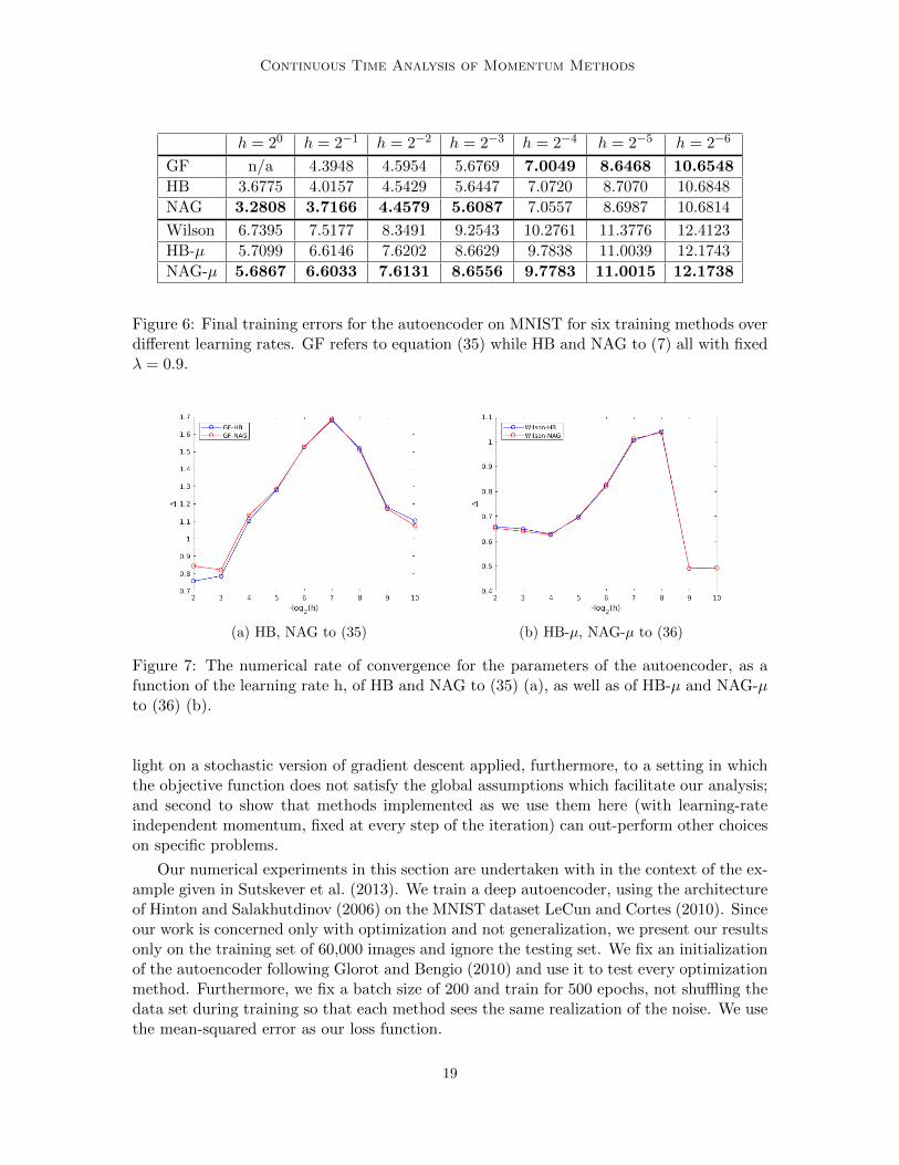
Figure 6: Final training errors for the autoencoder on MNIST for six training methods overdifferent learning rates. GF refers to equation (35) while HB and NAG to (7) all with fixedλ = 0.9.

(a) HB, NAG to (35) (b) HB-µ, NAG-µ to (36)

Figure 7: The numerical rate of convergence for the parameters of the autoencoder, as afunction of the learning rate h, of HB and NAG to (35) (a), as well as of HB-µ and NAG-µto (36) (b).

light on a stochastic version of gradient descent applied, furthermore, to a setting in whichthe objective function does not satisfy the global assumptions which facilitate our analysis;and second to show that methods implemented as we use them here (with learning-rateindependent momentum, fixed at every step of the iteration) can out-perform other choiceson specific problems.

Our numerical experiments in this section are undertaken with in the context of the ex-ample given in Sutskever et al. (2013). We train a deep autoencoder, using the architectureof Hinton and Salakhutdinov (2006) on the MNIST dataset LeCun and Cortes (2010). Sinceour work is concerned only with optimization and not generalization, we present our resultsonly on the training set of 60,000 images and ignore the testing set. We fix an initializationof the autoencoder following Glorot and Bengio (2010) and use it to test every optimizationmethod. Furthermore, we fix a batch size of 200 and train for 500 epochs, not shuffling thedata set during training so that each method sees the same realization of the noise. We usethe mean-squared error as our loss function.

19

Kovachki and Stuart

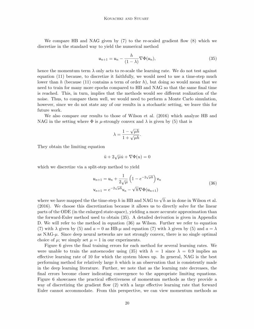
We compare HB and NAG given by (7) to the re-scaled gradient flow (8) which wediscretize in the standard way to yield the numerical method

un+1 = un −h

(1− λ)∇Φ(un), (35)

hence the momentum term λ only acts to re-scale the learning rate. We do not test againstequation (11) because, to discretize it faithfully, we would need to use a time-step muchlower than h (because (11) contains a term of order h), but doing so would mean that weneed to train for many more epochs compared to HB and NAG so that the same final timeis reached. This, in turn, implies that the methods would see different realization of thenoise. Thus, to compare them well, we would need to perform a Monte Carlo simulation,however, since we do not state any of our results in a stochastic setting, we leave this forfuture work.

We also compare our results to those of Wilson et al. (2016) which analyze HB andNAG in the setting where Φ is µ-strongly convex and λ is given by (5) that is

λ =1−√µh

1 +√µh.

They obtain the limiting equation

u+ 2√µu+∇Φ(u) = 0

which we discretize via a split-step method to yield

un+1 = un +1

2√µ

(1− e−2

√µh)vn

vn+1 = e−2√µhvn −

√h∇Φ(un+1)

(36)

where we have mapped the the time-step h in HB and NAG to√h as in done in Wilson et al.

(2016). We choose this discretization because it allows us to directly solve for the linearparts of the ODE (in the enlarged state-space), yielding a more accurate approximation thanthe forward-Euler method used to obtain (35). A detailed derivation is given in AppendixD. We will refer to the method in equation (36) as Wilson. Further we refer to equation(7) with λ given by (5) and a = 0 as HB-µ and equation (7) with λ given by (5) and a = λas NAG-µ. Since deep neural networks are not strongly convex, there is no single optimalchoice of µ; we simply set µ = 1 in our experiments.

Figure 6 gives the final training errors for each method for several learning rates. Wewere unable to train the autoencoder using (35) with h = 1 since λ = 0.9 implies aneffective learning rate of 10 for which the system blows up. In general, NAG is the bestperforming method for relatively large h which is an observation that is consistently madein the deep learning literature. Further, we note that as the learning rate decreases, thefinal errors become closer indicating convergence to the appropriate limiting equations.Figure 6 showcases the practical effectiveness of momentum methods as they provide away of discretizing the gradient flow (2) with a large effective learning rate that forwardEuler cannot accommodate. From this perspective, we can view momentum methods as

20


providing a more stable discretization to gradient flows in a manner illustrated by (20).Such a viewpoint informs the works Scieur et al. (2017); Betancourt et al. (2018); Zhanget al. (2018).

To further illustrate the point of convergence to the limiting equation, we compute thenumerical rate of convergence, defined in Section 2.3, as a function of h for the neuralnetwork parameters between (35) and HB and NAG as well as between (36) and HB-µ andNAG-µ. Figure 7 gives the results. We note that this rate is around 1 as predicted byour theory while the rate for (36) is around 0.5 which is also consistent with the theory inWilson et al. (2016).

6. Conclusion

Together, equations (8), (11) and (20) describe the dynamical systems which are approx-imated by momentum methods, when implemented with fixed momentum, in a mannermade precise by the four theorems in this paper. The insight obtained from these theoremssheds light on how momentum methods perform optimization tasks.

Acknowledgments

Both authors are supported, in part, by the US National Science Foundation (NSF) grantDMS 1818977, the US Office of Naval Research (ONR) grant N00014-17-1-2079, and the USArmy Research Office (ARO) grant W911NF-12-2-0022. Both authors are also grateful tothe anonymous reviewers for their invaluable suggestions which have helped to significantlystrengthen this work.

21

Kovachki and Stuart

Appendix A

Proof [of Theorem 2] Taylor expanding yields

un+1 = un + hλf(un) +O(h2)

andun = un−1 + hλf(un) +O(h2).

Hence(1 + λ)un − λun−1 = un + hλλf(un) +O(h2).

Subtracting the third identity from the first, we find that

un+1 − ((1 + λ)un − λun−1) = hf(un) +O(h2)

by noting λ− λλ = 1. Similarly,

a(un − un−1) = haλf(un) +O(h2)

hence Taylor expanding yields

f(un + a(un − un−1)) = f(un) + aDf(un)(un − un−1)

+ a2

∫ 1

0(1− s)D2f(un + sa(un − un−1))[un − un−1]2ds

= f(un) + haλDf(un)f(un) +O(h2).

From this, we conclude that

hf(un + a(un − un−1)) = hf(un) +O(h2)

henceun+1 = (1 + λ)un − λun−1 + hf(un + a(un − un−1)) +O(h2).

Define the error en := un − un then

en+1 = (1 + λ)en − λen−1 + h (f(un + a(un − un−1))− f(un + a(un − un−1))) +O(h2)

= (1 + λ)en − λen−1 + hMn((1 + a)en − aen−1) +O(h2)

where, from the mean value theorem, we have

Mn =

∫ 1

0Df(s(un + a(un − un−1)

)+(1− s

)(un + a(un − un−1)

))ds.

Now define the concatenation En+1 := [en+1, en] ∈ R2d then

En+1 = A(λ)En + hA(a)n En +O(h2)

where A(λ), A(a)n ∈ R2d×2d are the block matrices

A(λ) :=

[(1 + λ)I −λI

I 0I

], A(a)

n :=

[(1 + a)Mn −aMn

0I 0I

]22


with I ∈ Rd×d the identity. We note that A(λ) has minimal polynomial

µA(λ)(z) = (z − 1)(z − λ)

and is hence diagonalizable. Thus there is a norm on ‖ · ‖ on R2d such that its inducedmatrix norm ‖ · ‖m satifies ‖A(λ)‖m = ρ(A(λ)) where ρ : R2d×2d → R+ maps a matrix to itsspectral radius. Hence, since λ ∈ (0, 1), we have ‖A(λ)‖m = 1. Thus

‖En+1‖ ≤ (1 + h‖A(a)n ‖m)‖En‖+O(h2).

Then, by finite dimensional norm equivalence, there is a constant α > 0, independent of h,such that

‖A(a)n ‖m ≤ α

∥∥∥∥[1 + a −a0 0

]⊗Mn

∥∥∥∥2

= α√

2a2 + 2a+ 1‖Mn‖2

where ‖ · ‖2 denotes the spectral 2-norm. Using Assumption 1, we have

‖Mn‖2 ≤ B1

thus, letting c := α√

2a2 + 2a+ 1B1, we find

‖En+1‖ ≤ (1 + hc)‖En‖+O(h2).

Then, by Gronwall lemma,

‖En+1‖ ≤ (1 + hc)n‖E1‖n +(1 + hc)n+1 − 1

chO(h2)

= (1 + hc)n‖E1‖n +O(h)

noting that the constant in theO(h) term is bounded above in terms of T , but independentlyof h. Finally, we check the initial condition

E1 =

[u1 − u1

u0 − u0

]=

[h(λ− 1)f(u0) +O(h2)

0

]= O(h)

as desired.

Appendix B

Proof [of Theorem 3] Taylor expanding yields

un±1 = un ± hun +h2

2un ±

h3

2I±n

where

I±n =

∫ 1

0(1− s)2...

u ((n± s)h)ds.

23

Kovachki and Stuart

Then using equation (11)

un+1 − un − λ(un − un−1) = h(1− λ)un +h2

2(1 + λ)un +

h3

2(I+n − λI−n )

= hf(un) + h2a(1− λ)un +h3

2(I+n − λI−n ).

(37)

Similarly

a(un − un−1) = haun −h2

2aun +

h3

2aI−n

hence

f(un + a(un − un−1)) = f(un) + haDf(un)un −Df(un)

(h2

2aun −

h3

2aI−n

)+ Ifn

where

Ifn = a2

∫ 1

0(1− s)D2f(un + sa(un − un−1))[un − un−1]2ds.

Differentiating (11) yields

hαd3u

dt3+ (1− λ)

d2u

dt2= Df(u)

du

dt

hence

hf(un + a(un − un−1)) = hf(un) + h2a (hα...un + (1− λ)un)−Df(un)

(h3

2aun −

h4

2aI−n

)+ hIfn

= hf(un) + h2a(1− λ)un + h3aα...un −Df(un)

(h3

2aun −

h4

2aI−n

)+ hIfn .

Rearranging this we obtain an expression for hf(un) which we plug into equation (37) toyield

un+1 − un − λ(un − un−1) = hf(un + a(un − un−1)) + LTn

where

LTn =h3

2(I+n − λI−n )︸︷︷︸

O(hexp

(− (1−λ)

2αn))− h3aα

...un︸︷︷︸

O(hexp

(− (1−λ)

2αn)) +Df(un)

(h3

2aun −

h4

2aI−n

)︸︷︷︸

O(h2)

− hIfn︸︷︷︸O(h3)

.

The bounds (in braces) on the four terms above follow from employing Assumption 1 andLemma 8. From them we deduce the existence of constants K1,K2 > 0 independent of hsuch that

|LTn| ≤ hK1exp

(−(1− λ)

2αn

)+ h2K2.

We proceed similarly to the proof of Theorem 2, but with a different truncation errorstructure, and find the error satsifies

‖En+1‖ ≤ (1 + hc)‖En‖+ hK1exp

(−(1− λ)

2αn

)+ h2K2

24


where we abuse notation and continue to write K1,K2 when, in fact, the constants havechanged by use of finite-dimensional norm equivalence. Define K3 := K2/c then summingthis error, we find

‖En+1‖ ≤ (1 + hc)n‖E1‖+ hK3((1 + hc)n+1 − 1) + hK1

n∑j=0

(1 + hc)jexp

(−(1− λ)

2α(n− j)

)= (1 + hc)n‖E1‖+ hK3((1 + hc)n+1 − 1) + hK1Sn.

where

Sn = exp

(−(1− λ)

2αn

)(1 + hc)n+1exp(

(1−λ)2α (n+ 1)

)− 1

(1 + hc)exp(

1−λ2α

)− 1

.

Let T = nh then

Sn ≤(1 + hc)n+1exp

(1−λ2α

)(1 + hc)exp

(1−λ2α

)− 1

≤2exp

(cT + 1−λ

2α

)exp

(1−λ2α

)− 1

From this we deduce that

‖En+1‖ ≤ (1 + hc)n‖E1‖+O(h)

noting that the constant in theO(h) term is bounded above in terms of T , but independentlyof h. For the initial condition, we check

u1 − u1 = h(u′0 − f(u0)) +h2

2u0 +

h3

2I+

0

which is O(h) by Lemma 8. Putting the bounds together we obtain

sup0≤nh≤T

‖En‖ ≤ C(T )h.

Lemma 8 Suppose Assumption 1 holds and let u ∈ C3([0,∞);Rd) be the solution to

hαd2u

dt2+ (1− λ)

du

dt= f(u)

u(0) = u0,du

dt(0) = v0

for some u0, v0 ∈ Rd and α > 0 independent of h. Suppose h ≤ (1 − λ)2/2αB1 then there

are constants C(1), C(2)1 , C

(2)2 , C

(3)1 , C

(3)2 > 0 independent of h such that for any t ∈ [0,∞),

|u(t)| ≤ C(1),

|u(t)| ≤ C(2)1

hexp

(−(1− λ)

2hαt

)+ C

(2)2 ,

|...u (t)| ≤ C(3)1

h2exp

(−(1− λ)

2hαt

)+ C

(3)2 .

25

Kovachki and Stuart

One readily verifies that the result of Lemma 8 is tight by considering the one-dimensionalcase with f(u) = −u. This implies that the result of Theorem 3 cannot be improved withoutfurther assumptions.Proof [of Lemma 8] Define v := u then

v = − 1

hα((1− λ)v − f(u)) .

Define w := (1− λ)v − f(u) hence v = −(1/hα)w and u = v = λ(w + f(u)). Thus

w = (1− λ)v −Df(u)u

= −(1− λ)

hαw −Df(u)(λ(w + f(u))).

Hence we find

1

2

d

dt|w|2 = −(1− λ)

hα|w|2 − λ〈w,Df(u)w〉 − λ〈w,Df(u)f(u)〉

≤ −(1− λ)

hα|w|2 + λ|〈w,Df(u)w〉|+ λ|〈w,Df(u)f(u)〉|

≤ −(1− λ)

hα|w|2 + λB1|w|2 + λB0B1|w|

≤ −(1− λ)

hα|w|2 +

(1− λ)

2hα|w|2 + λB0B1|w|

= −(1− λ)

2hα|w|2 + λB0B1|w|

by noting that our assumption h ≤ (1− λ)2/2αB1 implies λB1 ≤ (1− λ)/2hα. Hence

d

dt|w| ≤ −(1− λ)

2hα|w|+ λB0B1

so, by Gronwall lemma,

|w(t)| ≤ exp

(−(1− λ)

2hαt

)|w(0)|+ 2hλ2αB0B1

(1− exp

(−(1− λ)

2hαt

))≤ exp

(−(1− λ)

2hαt

)|w(0)|+ hβ1

where we define β1 := 2λ2αB0B1. Hence

|u(t)| = |v(t)|

=1

hα|w(t)|

≤ 1

hαexp

(−(1− λ)

2hαt

)|w(0)|+ β1

α

=|(1− λ)v0 − f(u0)|

hαexp

(−(1− λ)

2hαt

)+β1

α

26


thus setting C(2)1 = |(1−λ)v0− f(u0)|/α and C

(2)1 = β1/α gives the desired result. Further,

|u(t)| = |v(t)|≤ λ(|w(t)|+ |f(u(t))|)≤ λ(|w(0)|+ hβ1 +B0)

hence we deduce the existence of C(1). Now define z := w then

z = −(1− λ)

hαz − λDf(u)z +G(u, v, w)

where we define G(u, v, w) := −λ(Df(u)(Df(u)v) +D2f(u)[v, w] +D2f(u)[Df(u)v, f(u)]).Using Assumption 1 and our bounds on w and v, we deduce that there is a constant C > 0independent of h such that

|G(u, v, w)| ≤ Chence

1

2

d

dt|z|2 = −(1− λ)

hα|z|2 − λ〈z,Df(u)z〉+ 〈z,G(u, v, w)〉

≤ −(1− λ)

hα|z|2 + λB1|z|2 + C|z|

≤ −(1− λ)

2hα|z|2 + C|z|

as before. Thus we findd

dt|z| ≤ −(1− λ)

2hα|z|+ C

so, by Gronwall lemma,

|z(t)| ≤ exp

(−(1− λ)

2hαt

)|z(0)|+ hβ2

where we define β2 := 2λαC. Recall that

...u = v = − 1

hαw = − 1

hαz

and note

|z(0)| ≤ (1− λ)|(1− λ)v0 − f(u0)|hα

+B1|v0|

hence we find

|...u (t)| ≤(

(1− λ)|(1− λ)v0 − f(u0)

h2α2+B1|v0|hα

)exp

(−(1− λ)

2hαt

)+β2

α.

Thus we deduce that there is a constant C(3)1 > 0 independent of h such that

|...u (t)| ≤ C(3)1

h2exp

(−(1− λ)

2hαt

)+ C

(3)2

as desired where C(3)2 = β2/α.

27

Kovachki and Stuart

Appendix C.

For the results of Section 4 we make the following assumption on the size of h. Recall firstthat by Assumption 1 there are constants B0, B1, B2 > 0 such that

‖Dj−1f‖ = ‖DjΦ‖ ≤ Bj−1

for j = 1, 2, 3.

Lemma 9 Suppose h > 0 is small enough such that

λ+ hB1(a+ λλ) < 1

then there is a τ1 > 0 such that for any γ ∈ [τ1,∞)

(λ+ hB1(a+ λλ))γ + λB0B1(a+ λ) ≤ γ. (38)

Using Lemma 9 fix γ ∈ [τ1,∞) and define the constants

K1 := λB0 + hγ

K3 := B0 + λK1

α2 := h2(λ+ haB1),

α1 := λ− 1 + h(B1(λ+ a(1 + hλB1)) + λλ(B1 + hB2K3) + ha(aB2K1 +B1λ(B1 + hB2K3)

),

α0 := aB2K1(1 + haλB1) + λ(aB21 +B2K3) + λ2B1(1 + haB1)(B1 + hB2K3).

(39)

Lemma 10 Suppose h > 0 is small enough such that

α21 > 4α2α0, α1 < 0

then there are τ±2 > 0 such that for any δ ∈ (τ−2 , τ+2 ]

α2δ2 + α1δ + α0 ≤ 0. (40)

Using Lemma 10 fix δ ∈ (τ−2 , τ+2 ]. We make the following assumption on the size of the

learning rate h which is achievable since λ ∈ (0, 1).

Assumption 11 Let Assumption 1 hold and suppose h > 0 is small enough such that theassumptions of Lemmas 9, 10 hold. Define K2 := λB1 + hδ and suppose h > 0 is smallenough such that

c := h(λK2 +B1(1 + haK2)) < 1. (41)

Define constants

Q1 := λδ + a(B1K2 +B2K1(1 + haK2)) + λ((B1 + hB2K3)(λK2 +B1(1 + haK2)) +B2K3),

Q2 := h(a(B1 + haB2K1) + λ(λ+ haB1)(B1 + hB2K3)),

Q3 := h(λK2 +B1(1 + haK2)),

µ := λ+Q2 +h2(λ+ haB1)Q1

1−Q3.

(42)

28


Suppose h > 0 is small enough such that

Q3 < 1, µ < 1. (43)

Lastly assume h > 0 is small enough such that

λ+ h2λδ < 1. (44)

Proof [of Lemma 9.] Since λ+ hB1(a+ λλ) < 1 and λB0B1(a+ λ) > 0 the line defined by

(λ+ hB1(a+ λλ))γ + λB0B1(a+ λ)

will intersect the identity line at a positive γ and lie below it thereafter. Hence setting

τ1 =λB0B1(a+ λ)

1− λ+ hB1(a+ λλ)

completes the proof.

Proof [of Lemma 10.] Note that since α2 > 0, the parabola defined by

α2δ2 + α1δ + α0

is upward-pointing and has roots

ζ± =−α1 ±

√α2

1 − 4α2α0

2α2.

Since α21 > 4α2α0, ζ± ∈ R with ζ+ 6= ζ−. Since α1 < 0, ζ+ > 0 hence setting τ+

2 = ζ+ andτ−2 = max{0, ζ−} completes the proof.

The following proof refers to four lemmas whose statement and proof follow it.

Proof [of Theorem 5.] Define τ > 0 as the maximum h such that Assumption 11 holds. Thecontraction mapping principle together with Lemmas 13, 14, and 15 show that the operatorT defined by (29) and (30) has a unique fixed point in Γ. Hence, from its definition andequation (23b), we immediately obtain the existence result. We now show exponentialattractivity. Recall the definition of the operator T namely equations (29), (30):

p = ξ + hzg(ξ)

(Tg)(p) = λg(ξ) + aI(1)g (ξ)− λI(2)

g (ξ).

Let g ∈ Γ be the fixed point of T and set

p = un + hzg(un)

g(p) = λg(un) + aI(1)g (un)− λI(2)

g (un).

29

Kovachki and Stuart

Then

|vn+1 − λf(un+1)− hg(un+1)| ≤ |vn+1 − λf(un+1)− hg(p)|+ h|g(p)− g(un+1)|≤ |vn+1 − λf(un+1)− hg(p)|+ hδ|p− un+1|

since g ∈ Γ. Since, by definition,

vn+1 = λvn + f(un + havn)

we have,

|vn+1 − λf(un+1)− hg(p)| = |λvn + f(un + havn)− λf(un+1)− h(λg(un) + aI(1)g (un)− λI(2)

g (un))|= λ|vn − λf(un)− hg(un)|

by noting that

f(un + havn) = f(un) + haI(1)g (un)

f(un+1) = f(un) + hI(2)g (un).

From definition,


thus

|p− un+1| = |un + hzg(un)− un − hλvn − hf(un + havn)|= h|λ(λf(un) + hg(un)) + f(un + havn)− λvn − f(un + havn)|= hλ|vn − λf(un)− hg(un)|.

Hence

|vn+1 − λf(un+1)− hg(un+1)| ≤ (λ+ h2λδ)|vn − λf(un)− hg(un)|

as desired. By Assumption 11, λ+ h2λδ < 1.

The following lemma gives basic bounds which are used in the proof of Lemmas 13, 14,15.

30


Lemma 12 Let g, q ∈ Γ and ξ, η ∈ Rd then the quantities defined by (24), (25), (27), (28)satisfy the following:

|wg(ξ)| ≤ K1,

|wg(ξ)− wg(η)| ≤ K2|ξ − η|,|wg(ξ)− wq(ξ)| ≤ h|g(ξ)− q(ξ)|,

|zg(ξ)| ≤ K3,

|zg(ξ)− zg(η)| ≤ (λK2 +B1 (1 + haK2)) |ξ − η|,|zg(ξ)− zq(ξ)| ≤ h (λ+ haB1) |g(ξ)− q(ξ)|,

|I(1)g (ξ)| ≤ B1K1,

|I(1)g (ξ)− I(1)

g (η)| ≤ (B1K2 +B2K1(1 + haK2))|ξ − η|,

|I(1)g (ξ)− I(1)

q (ξ)| ≤ h(B1 + haB2K1)|g(ξ)− q(ξ)|,

|I(2)g (ξ)| ≤ B1K3

|I(2)g (ξ)− I(2)

g (η)| ≤ ((B1 + hB2K3)(λK2 +B1(1 + haK2)) +B2K3)|ξ − η|,

|I(2)g (ξ)− I(2)

q (ξ)| ≤ h(λ+ hB1a)(B1 + hB2K3)|g(ξ)− q(ξ)|.

Proof These bounds relay on applications of the triangle inequality together with bound-edness of f and its derivatives as well as the fact that functions in Γ are bounded and

Lipschitz. To illustrate the idea, we will prove the bounds for wg, wq, I(1)g , and I

(1)q . To that

end,

|wg(ξ)| = |λf(ξ) + hg(ξ)|≤ λ|f(ξ)|+ h|g(ξ)|≤ λB0 + hγ

= K1

establishing the first bound. For the second,

|wg(ξ)− wg(η)| ≤ λ|f(ξ)− f(η)|+ h|g(ξ)− g(η)|≤ λB1|ξ − η|+ hδ|ξ − η|= K2|ξ − η|

as desired. Finally,

|wg(ξ)− wq(ξ)| = |λf(ξ) + hg(ξ)− λf(ξ)− hq(ξ)|= h|g(ξ)− q(ξ)|

as desired. We now turn to the bounds for I(1)g , I

(1)q ,

|I(1)g (ξ)| ≤

∫ 1

0|Df(ξ + shawg(ξ))||wg(ξ)|ds

≤∫ 1

0B1K1ds

= B1K1

31

Kovachki and Stuart

establishing the first bound. For the second bound,

|I(1)g (ξ)− I(1)

g (η)| ≤∫ 1

0|Df(ξ + shawg(ξ))wg(ξ)−Df(η + shawg(η))wg(ξ)|ds

+

∫ 1

0|Df(η + shawg(η))wg(ξ)−Df(η + shawg(η))wg(η)|ds

≤ K1B2

∫ 1

0(|ξ − η|+ sha|wg(ξ)− wg(η)|)ds+B1|wg(ξ)− wg(η)|

≤ K1B2(|ξ − η|+ haK2|ξ − η|) +B1K2|ξ − η|= (B1K2 +B2K1(1 + haK2))|ξ − η|

as desired. Finally

|I(1)g (ξ)− I(1)

q (ξ)| ≤∫ 1

0|Df(ξ + shawg(ξ))wg(ξ)−Df(ξ + shawg(ξ))wq(ξ)|ds

+

∫ 1

0|Df(ξ + shawg(ξ))wq(ξ)−Df(ξ + shawq(ξ))wq(ξ)|ds

≤ B1

∫ 1

0|wg(ξ)− wq(ξ)|ds+K1B2

∫ 1

0|ξ + shawg(ξ)− ξ − shawq(ξ)|ds

≤ hB1|g(ξ)− q(ξ)|+ h2aB2K1|g(ξ)− q(ξ)|= h(B1 + haB2K1)|g(ξ)− q(ξ)|

as desired. The bounds for zg, zq, I(2)g , and I

(2)q follow similarly.

We also need the following three lemmas:

Lemma 13 Suppose Assumption 11 holds. For any g ∈ Γ and p ∈ Rd there exists a uniqueξ ∈ Rd satisfying (29).

Lemma 14 Suppose Assumption 11 holds. The operator T defined by (30) satisfies T : Γ→ Γ.

Lemma 15 Suppose Assumption 11 holds. For any g1, g2 ∈ Γ, we have

‖Tg1 − Tg2‖Γ ≤ µ‖g1 − g2‖Γ

where µ < 1.

Now we prove these three lemmas.Proof [of Lemma 13.] Consider the iteration of the form

ξk+1 = p− hzg(ξk).

For any two sequences {ξk}, {ηk} generated by this iteration we have, by Lemma 12,

|ξk+1 − ηk+1| ≤ h|zg(ηk)− zg(ξk)|≤ h(λK2 +B1(1 + haK2))|ξk − ηk|= c|ξk − ηk|

32


which is a contraction by (41).

Proof [of Lemma 14.] Let g ∈ Γ and p ∈ Rd then by Lemma 13 there is a unique ξ ∈ Rdsuch that (29) is satisfied. Then

|(Tg)(p)| ≤ λ|g(ξ)|+ a|I(1)g (ξ)|+ λ|I(2)

g (ξ)|≤ λγ + aB1(λB0 + hγ) + λB1(λ(λB0 + hγ) +B0)

= (λ+ hB1(a+ λλ))γ + λB0B1(a+ λ)

≤ γ

with the last inequality following from (38).Let p1, p2 ∈ Rd then, by Lemma 13, there exist ξ1, ξ2 ∈ Rd such that (29) is satisfied

with p = {p1, p2}. Hence, by Lemma 12,

|(Tg)(p1)− (Tg)(p2)| ≤ λ|g(ξ1)− g(ξ2)|+ a|I(1)g (ξ1)− I(1)

g (ξ2)|+ λ|I(2)g (ξ1)− I(2)

g (ξ2)|≤ K|ξ1 − ξ2|

where we define

K := λδ + a(B1K2 +B2K1(1 + haK2)) + λ((B1 + hB2K3)(λK2 +B1(1 + haK2)) +B2K3).

Now, using (29) and the proof of Lemma 13,

|ξ1 − ξ2| ≤ |p1 − p2|+ h|zg(ξ1)− zg(ξ2)|≤ |p1 − p2|+ c|ξ1 − ξ2|.

Since c < 1 by (41), we obtain

|ξ1 − ξ2| ≤1

1− c|p1 − p2|

thus

|(Tg)(p1)− (Tg)(p2)| ≤ K

1− c|p1 − p2| ≤ δ|p1 − p2|.

To see the last inequality, we note that

K

1− c≤ δ ⇐⇒ K − δ(1− c) ≤ 0

and K − δ(1− c) = α2δ2 + α1δ + α0 by (39) hence (40) gives the desired result.

Proof [of Lemma 15.] By Lemma 13, for any p ∈ Rd and g1, g2 ∈ Γ, there are ξ1, ξ2 ∈ Rdsuch that

p = ξj + hzgj (ξj)

(Tgj)(p) = λgj(ξj) + aI(1)gj (ξj)− λI(2)

gj (ξj)

33

Kovachki and Stuart

for j = 1, 2. Then

|(Tg1)(p)− (Tg2)(p)| ≤ λ|g1(ξ1)− g2(ξ2)|+ a|I(1)g1 (ξ1)− I(1)

g2 (ξ2)|+ λ|I(2)g1 (ξ1)− I(2)

g2 (ξ2)|.

Note that

|g1(ξ1)− g2(ξ2)| = |g1(ξ1)− g2(ξ2)− g2(ξ1) + g2(ξ1)|≤ |g1(ξ1)− g2(ξ1)|+ δ|ξ1 − ξ2|.

Similarly, by Lemma 12,

|I(1)g1 (ξ1)− I(1)

g2 (ξ2)| = |I(1)g1 (ξ1)− I(1)

g2 (ξ2)− I(1)g2 (ξ1) + I(1)

g2 (ξ1)|

≤ |I(1)g1 (ξ1)− I(1)

g2 (ξ1)|+ |I(1)g2 (ξ1)− I(1)

g2 (ξ2)|≤ h(B1 + haB2K1)|g1(ξ1)− g2(ξ1)|+ (B1K2 +B2K1(1 + haK2))|ξ1 − ξ2|

Finally,

|I(2)g1 (ξ1)− I(2)

g2 (ξ2)| = |I(2)g1 (ξ1)− I(2)

g2 (ξ2)− I(2)g2 (ξ1) + I(2)

g2 (ξ1)|

≤ |I(2)g1 (ξ1)− I(2)

g2 (ξ1)|+ |I(2)g2 (ξ1)− I(2)

g2 (ξ2)|≤ h(λ+ hB1a)(B1 + hB2K3)|g1(ξ1)− g2(ξ1)|++ ((B1 + hB2K3)(λK2 +B1(1 + haK2)) +B2K3)|ξ1 − ξ2|

Putting these together and using (42), we obtain

|(Tg1)(p)− (Tg2)(p)| ≤ (λ+Q2)|g1(ξ1)− g2(ξ1)|+Q1|ξ1 − ξ2|.

Now, by Lemma 12,

|ξ1 − ξ2| ≤ h|zg1(ξ1)− zg2(ξ2)− zg2(ξ1) + zg2(ξ1)|≤ h(|zg1(ξ1)− zg2(ξ1)|+ |zg2(ξ1)− zg2(ξ2)|)≤ h2(λ+ haB1)|g1(ξ)− g2(ξ1)|+ h(λK2 +B1(1 + haK2))|ξ1 − ξ2|= h2(λ+ haB1)|g1(ξ)− g2(ξ1)|+Q3|ξ1 − ξ2|

using (42). Since, by (43), Q3 < 1, we obtain

|ξ1 − ξ2| ≤h2(λ+ haB1)

1−Q3|g1(ξ1)− g2(ξ1)|

and thus

|(Tg1)(p)− (Tg2)(p)| ≤(λ+Q2 +

h2(λ+ haB1)Q1

1−Q3

)|g1(ξ1)− g2(ξ1)|

= µ|g1(ξ1)− g2(ξ1)|

by (42). Taking the supremum over ξ1 then over p gives the desired result. Since µ < 1 by(43), we obtain that T is a contraction on Γ.

34


Appendix D

We consider the equation

u+ 2√µu+∇Φ(u) = 0

u(0) = u0, u(0) = v0.

Set v = u then we have [uv

]=

[v

−2√µv −∇Φ(u)

].

Define the maps

f1(u, v) :=

[v

−2√µv

], f2(u, v) :=

[0

−∇Φ(u)

]then [

uv

]= f1(u, v) + f2(u, v).

We first solve the system [uv

]= f1(u, v).

Clearly

v(t) = e−2√µtv0

hence

u(t) = u0 +

∫ t

0e−2√µsv0 ds

= u0 +1

2√µ

(1− e−2

√µt)v0.

This gives us the flow map

ψ1(u, v; t) =

[u + 1

2√µ

(1− e−2

√µt)v

e−2√µtv

].

We now solve the system [uv

]= f2(u, v).

Clearly

u(t) = u0

hence

v(t) = v0 − t∇Φ(u0).

This gives us the flow map

ψ2(u, v; t) =

[u

v − t∇Φ(u)

].

35

Kovachki and Stuart

The composition of the flow maps is then

(ψ2 ◦ ψ1)(u, v; t) =

[u + 1

2√µ

(1− e−2

√µt)v

e−2√µtv − t∇Φ

(u + 1

2√µ

(1− e−2

√µt)v)] .

Mapping t to the time-step√h gives the numerical method (36).

References

Martın Abadi, Ashish Agarwal, Paul Barham, Eugene Brevdo, Zhifeng Chen, Craig Citro,Greg S. Corrado, Andy Davis, Jeffrey Dean, Matthieu Devin, Sanjay Ghemawat, IanGoodfellow, Andrew Harp, Geoffrey Irving, Michael Isard, Yangqing Jia, Rafal Joze-fowicz, Lukasz Kaiser, Manjunath Kudlur, Josh Levenberg, Dandelion Mane, RajatMonga, Sherry Moore, Derek Murray, Chris Olah, Mike Schuster, Jonathon Shlens,Benoit Steiner, Ilya Sutskever, Kunal Talwar, Paul Tucker, Vincent Vanhoucke, VijayVasudevan, Fernanda Viegas, Oriol Vinyals, Pete Warden, Martin Wattenberg, MartinWicke, Yuan Yu, and Xiaoqiang Zheng. TensorFlow: Large-scale machine learning onheterogeneous systems, 2015. URL https://www.tensorflow.org/. Software availablefrom tensorflow.org.

Dimitris Bertsimas, John Tsitsiklis, et al. Simulated annealing. Statistical science, 8(1):10–15, 1993.

Michael Betancourt, Michael I. Jordan, and Ashia C. Wilson. On symplectic optimization,2018.

Jack Carr. Applications of centre manifold theory, volume 35. Springer Science & BusinessMedia, 2012.

Philippe Chartier, Ernst Hairer, and Gilles Vilmart. Numerical integrators based on modi-fied differential equations. Mathematics of computation, 76(260):1941–1953, 2007.

Aymeric Dieuleveut, Alain Durmus, and Francis Bach. Bridging the gap between constantstep size stochastic gradient descent and markov chains. arXiv preprint arXiv:1707.06386,2017.

John Duchi, Elad Hazan, and Yoram Singer. Adaptive subgradient methods for onlinelearning and stochastic optimization. J. Mach. Learn. Res., 12:2121–2159, July 2011.ISSN 1532-4435. URL http://dl.acm.org/citation.cfm?id=1953048.2021068.

Yuanyuan Feng, Lei Li, and Jian-Guo Liu. Semigroups of stochastic gradient descent andonline principal component analysis: properties and diffusion approximations. Commu-nications in Mathematical Sciences, 16(3):777–789, 2018.

Sebastien Gadat, Fabien Panloup, Sofiane Saadane, et al. Stochastic heavy ball. ElectronicJournal of Statistics, 12(1):461–529, 2018.

36

https://www.tensorflow.org/

http://dl.acm.org/citation.cfm?id=1953048.2021068


Stuart Geman and Donald Geman. Stochastic relaxation, gibbs distributions, and thebayesian restoration of images. In Readings in computer vision, pages 564–584. Elsevier,1987.

Xavier Glorot and Yoshua Bengio. Understanding the difficulty of training deep feedforwardneural networks. In In Proceedings of the International Conference on Artificial Intel-ligence and Statistics (AISTATS’10). Society for Artificial Intelligence and Statistics,2010.

Ian Goodfellow, Yoshua Bengio, and Aaron Courville. Deep Learning. MIT Press, 2016.http://www.deeplearningbook.org.

DF Griffiths and JM Sanz-Serna. On the scope of the method of modified equations. SIAMJournal on Scientific and Statistical Computing, 7(3):994–1008, 1986.

Kaiming He, Xiangyu Zhang, Shaoqing Ren, and Jian Sun. Deep residual learning forimage recognition. 2016 IEEE Conference on Computer Vision and Pattern Recognition(CVPR), pages 770–778, 2016.

Geoffrey Hinton and Ruslan Salakhutdinov. Reducing the dimensionality of data with neuralnetworks. Science, 313(5786):504 – 507, 2006.

Morris W Hirsch, Charles Chapman Pugh, and Michael Shub. Invariant manifolds, volume583. Springer, 2006.

Bin Hu and Laurent Lessard. Dissipativity theory for nesterov’s accelerated method. InProceedings of the 34th International Conference on Machine Learning-Volume 70, pages1549–1557. JMLR. org, 2017.

Diederik P. Kingma and Jimmy Ba. Adam: A method for stochastic optimization. CoRR,abs/1412.6980, 2014. URL http://arxiv.org/abs/1412.6980.

Harold J Kushner. Asymptotic global behavior for stochastic approximation and diffusionswith slowly decreasing noise effects: global minimization via monte carlo. SIAM Journalon Applied Mathematics, 47(1):169–185, 1987.

Harold Joseph Kushner and Dean S Clark. Stochastic approximation methods for constrainedand unconstrained systems, volume 26. Springer Science & Business Media, 2012.

Yann LeCun and Corinna Cortes. MNIST handwritten digit database. 2010. URL http:

//yann.lecun.com/exdb/mnist/.

Yann LeCun, Yoshua Bengio, and Geoffrey E. Hinton. Deep learning. Nature, 521(7553):436–444, 2015. doi: 10.1038/nature14539. URL https://doi.org/10.1038/

nature14539.

Laurent Lessard, Benjamin Recht, and Andrew Packard. Analysis and design of optimiza-tion algorithms via integral quadratic constraints. SIAM Journal on Optimization, 26(1):57–95, 2016.

37

http://www.deeplearningbook.org

http://arxiv.org/abs/1412.6980

http://yann.lecun.com/exdb/mnist/

http://yann.lecun.com/exdb/mnist/

https://doi.org/10.1038/nature14539

https://doi.org/10.1038/nature14539

Kovachki and Stuart

Qianxiao Li, Cheng Tai, and Weinan E. Stochastic modified equations and adaptive stochas-tic gradient algorithms. In Doina Precup and Yee Whye Teh, editors, Proceedings of the34th International Conference on Machine Learning, volume 70 of Proceedings of MachineLearning Research, pages 2101–2110, International Convention Centre, Sydney, Australia,06–11 Aug 2017. PMLR.

Nicolas Loizou and Peter Richtarik. Linearly convergent stochastic heavy ball method forminimizing generalization error. arXiv preprint arXiv:1710.10737, 2017.

Jonathan C Mattingly, Andrew M Stuart, and Michael V Tretyakov. Convergence of nu-merical time-averaging and stationary measures via poisson equations. SIAM Journal onNumerical Analysis, 48(2):552–577, 2010.

Yurii Nesterov. A method of solving a convex programming problem with convergence rateo(1/k2). Soviet Mathematics Doklady, 27(2):372–376, 1983.

Yurii Nesterov. Introductory Lectures on Convex Optimization: A Basic Course. SpringerPublishing Company, Incorporated, 1 edition, 2014. ISBN 1461346916, 9781461346913.

Adam Paszke, Sam Gross, Soumith Chintala, Gregory Chanan, Edward Yang, ZacharyDeVito, Zeming Lin, Alban Desmaison, Luca Antiga, and Adam Lerer. Automatic dif-ferentiation in pytorch. In NIPS-W, 2017.

Grigorios Pavliotis and Andrew Stuart. Multiscale Methods: Averaging and Homogenization,volume 53. 01 2008. doi: 10.1007/978-0-387-73829-1.

Boris Polyak. Some methods of speeding up the convergence of iteration methods. UssrComputational Mathematics and Mathematical Physics, 4:1–17, 12 1964. doi: 10.1016/0041-5553(64)90137-5.

Boris T. Polyak. Introduction to optimization. New York: Optimization Software, Inc.,1987.

Ning Qian. On the momentum term in gradient descent learning algorithms. Neural Netw.,12(1):145–151, January 1999. ISSN 0893-6080. doi: 10.1016/S0893-6080(98)00116-6.URL http://dx.doi.org/10.1016/S0893-6080(98)00116-6.

Herbert Robbins and Sutton Monro. A stochastic approximation method. Ann. Math.Statist., 22(3):400–407, 09 1951. doi: 10.1214/aoms/1177729586. URL https://doi.

org/10.1214/aoms/1177729586.

D. E. Rumelhart, G. E. Hinton, and R. J. Williams. Parallel distributed processing: Ex-plorations in the microstructure of cognition, vol. 1. chapter Learning Internal Represen-tations by Error Propagation, pages 318–362. MIT Press, Cambridge, MA, USA, 1986.ISBN 0-262-68053-X. URL http://dl.acm.org/citation.cfm?id=104279.104293.

Damien Scieur, Vincent Roulet, Francis Bach, and Alexandre d’Aspremont. Integrationmethods and optimization algorithms. In Advances in Neural Information ProcessingSystems, pages 1109–1118, 2017.

38

http://dx.doi.org/10.1016/S0893-6080(98)00116-6

https://doi.org/10.1214/aoms/1177729586

https://doi.org/10.1214/aoms/1177729586



Bin Shi, Simon S Du, Michael I Jordan, and Weijie J Su. Understanding the accelerationphenomenon via high-resolution differential equations. arXiv preprint arXiv:1810.08907,2018.

Andrew Stuart and Anthony R Humphries. Dynamical systems and numerical analysis,volume 2. Cambridge University Press, 1998.

MA Styblinski and T-S Tang. Experiments in nonconvex optimization: stochastic approxi-mation with function smoothing and simulated annealing. Neural Networks, 3(4):467–483,1990.

Weijie Su, Stephen Boyd, and Emmanuel Candes. A differential equation formodeling nesterov’s accelerated gradient method: Theory and insights. InZ. Ghahramani, M. Welling, C. Cortes, N. D. Lawrence, and K. Q. Wein-berger, editors, Advances in Neural Information Processing Systems 27, pages2510–2518. Curran Associates, Inc., 2014. URL http://papers.nips.cc/paper/

5322-a-differential-equation-for-modeling-nesterovs-accelerated-gradient-method-theory-and-insights.

pdf.

Ilya Sutskever, James Martens, George Dahl, and Geoffrey Hinton. On the importance ofinitialization and momentum in deep learning. In Proceedings of the 30th InternationalConference on International Conference on Machine Learning - Volume 28, ICML’13,pages III–1139–III–1147. JMLR.org, 2013. URL http://dl.acm.org/citation.cfm?

id=3042817.3043064.

T. Tieleman and G. Hinton. Lecture 6.5—RmsProp: Divide the gradient by a runningaverage of its recent magnitude. COURSERA: Neural Networks for Machine Learning,2012.

Stephen Wiggins. Normally hyperbolic invariant manifolds in dynamical systems, volume105. Springer Science & Business Media, 2013.

Ashia C. Wilson, Benjamin Recht, and Michael I. Jordan. A lyapunov analysis of momentummethods in optimization. CoRR, abs/1611.02635, 2016. URL http://arxiv.org/abs/

1611.02635.

Ashia C Wilson, Rebecca Roelofs, Mitchell Stern, Nati Srebro, and BenjaminRecht. The marginal value of adaptive gradient methods in machine learning. InI. Guyon, U. V. Luxburg, S. Bengio, H. Wallach, R. Fergus, S. Vishwanathan,and R. Garnett, editors, Advances in Neural Information Processing Systems 30,pages 4148–4158. Curran Associates, Inc., 2017. URL http://papers.nips.cc/paper/

7003-the-marginal-value-of-adaptive-gradient-methods-in-machine-learning.

pdf.

Tianbao Yang, Qihang Lin, and Zhe Li. Unified convergence analysis of stochastic momen-tum methods for convex and non-convex optimization. arXiv preprint arXiv:1604.03257,2016.

39

http://papers.nips.cc/paper/5322-a-differential-equation-for-modeling-nesterovs-accelerated-gradient-method-theory-and-insights.pdf







http://papers.nips.cc/paper/7003-the-marginal-value-of-adaptive-gradient-methods-in-machine-learning.pdf



Kovachki and Stuart

Jingzhao Zhang, Aryan Mokhtari, Suvrit Sra, and Ali Jadbabaie. Direct runge-kutta dis-cretization achieves acceleration. In Proceedings of the 32nd International Conference onNeural Information Processing Systems, NIPS’18, page 3904–3913, Red Hook, NY, USA,2018. Curran Associates Inc.

40

Documents

Continuous Time Analysis of Momentum Methods