Embed Size (px)
Citation preview

8/13/2019 Continuous-State Graphical Models for Object Localization, Pose Estimation and Tracking
http://slidepdf.com/reader/full/continuous-state-graphical-models-for-object-localization-pose-estimation 1/220
Continuous-state Graphical Models for Object Localization, Pose
Estimation and Tracking
by
Leonid Sigal
B. A., Boston University, 1999
M. A., Boston University, 1999
Sc. M., Brown University, 2003
Submitted in partial fulfillment of the requirements
for the Degree of Doctor of Philosophy in the
Department of Computer Science at Brown University
Providence, Rhode Island
May 2008

8/13/2019 Continuous-State Graphical Models for Object Localization, Pose Estimation and Tracking
http://slidepdf.com/reader/full/continuous-state-graphical-models-for-object-localization-pose-estimation 2/220
c Copyright 2003, 2004, 2006, 2008 by Leonid Sigal

8/13/2019 Continuous-State Graphical Models for Object Localization, Pose Estimation and Tracking
http://slidepdf.com/reader/full/continuous-state-graphical-models-for-object-localization-pose-estimation 3/220
This dissertation by Leonid Sigal is accepted in its present form by
the Department of Computer Science as satisfying the dissertation requirement
for the degree of Doctor of Philosophy.
Date
Michael J. Black, Director
Recommended to the Graduate Council
Date
William T. Freeman, Reader
(Electrical Engineering and Computer Science)
Massachusetts Institute of Technology
Date
John F. Hughes, Reader
(Department of Computer Science)
Date
David Mumford, Reader
(Department of Applied Mathematics)
Approved by the Graduate Council
Date
Sheila Bonde
Dean of the Graduate School
iii

8/13/2019 Continuous-State Graphical Models for Object Localization, Pose Estimation and Tracking
http://slidepdf.com/reader/full/continuous-state-graphical-models-for-object-localization-pose-estimation 4/220
VITA
Leonid Sigal was born on May 23, 1977 in Kiev, Ukraine. He is a Ph.D. candidate under the supervision
of Michael J. Black at Brown University; he received his B.Sc. degrees in Computer Science and Mathe-
matics from Boston University (1999), his M.A. from Boston University (1999), and his M.S. from Brown
University (2003). From 1999 to 2001, he worked as a senior vision engineer at Cognex Corporation, where
he developed industrial vision applications for pattern analysis and verification. In 2002, he spent a semester
as a research intern at Siemens Corporate Research (SCR) working on autonomous obstacle detection and
avoidance for vehicle navigation. During the summers of 2005 and 2006, he worked as a research intern at
Intel Applications Research Lab (ARL) on human pose estimation and tracking. His work received the Best
Paper Award at the Articulate Motion and Deformable Objects Conference in 2006 (with Michael J. Black).
Leonid’s research interests are primarily in computer vision and machine learning, including human motion
analysis, graphical models, probabilistic and hierarchical inference.
iv

8/13/2019 Continuous-State Graphical Models for Object Localization, Pose Estimation and Tracking
http://slidepdf.com/reader/full/continuous-state-graphical-models-for-object-localization-pose-estimation 5/220
ACKNOWLEDGEMENTS
First and foremost, I would like to thank my advisor and mentor Michael J. Black for his attentive supervision
during my six years at Brown University. Michael provided me with a wealth of expertise and knowledge.
He taught me how to choose and approach challenging problems and how to formulate a clear scientific
argument. His enthusiasm and ability to engage students in interesting problems has served as an inspiration
to me. As an advisor, Michael struck a perfect balance of providing help to me where and when it was needed,
yet allowing me the freedom to grow as an independent researcher.
I am also grateful to all members of Browns’ computer vision group and graduate community for helpful
discussions, collaborations and a friendly environment that allowed me to conduct this research. I would
specifically like to thank Stefan Roth for being a congenial colleague and for the advice that he has given me
over the years; Alexandru Balan for a variety of collaborations and for introducing me to the SC APE model.
I would also like to thank Alexundru for his entertaining personal stories and the companionship during
numerous conference travels and internships. I would also like to mention other group members who have
indirectly affected this thesis: Gregory Shakhnarovich, Payman Yadollahpur and Frank Wood. In addition,
I want to thank Chad Jenkins and his students for introducing me to robotics and physics-based simulation,
while this has no direct relation to this thesis, it has affected my overall research agenda.
The ideas developed in this thesis have also benefited from numerous external collaborations. I would
like to thank Michael Isard for his early input and discussions on Particle Massage Passing (PAMPAS), which
is at the core of this thesis. I would also like to thank Alex Ihler and Eric Sudderth for interesting discussions
on the relations between Non-parametric Belief Propagation (NBP), developed by them, and P AMPAS. In
addition, I would like to thank Dorin Comaniciu and Ying Zhu from Siemens Corporate Research (SCR) for
the mentorship they provided me during my five month internship in Princeton, NJ. As part of my internship,I
was able to extend my prior work on articulated pose estimation and tracking to the generic obstacle detection
domain (for autonomous vehicle navigation); this gave rise to the results presented in Chapter 4. I would also
like to thank, Horst Haussecker, who has hosted me as a Research Intern at Intels Applications Research
Laboratory (ARL) in Santa Clara, CA for two summers in 2006 and 2007. Horst provided me with an
invaluable environment and freedom to pursue research of my own personal interest. The collaborations
with various people in the ARL group, in particular Nizhny Novgorod’s team has benefited this thesis in
many practical aspects. Much of the experiments presented in Chapter 5 would not be possible (or as easily
attained) without their help. Hence, I would like to thank all members of the Intel Research group with whom
I had a chance to interact and collaborate with during my visits: Adam Seeger, Oscar Nestares, Jean-Yves
Bouguet, Konstantin Rodyushkin (Nizhny Novgorod, Russia) and Alexander Kuranov (Nizhny Novgorod,
Russia).
Moreover, I am grateful to members of my thesis committee, William Freeman, John Hughes (Spike)
v

8/13/2019 Continuous-State Graphical Models for Object Localization, Pose Estimation and Tracking
http://slidepdf.com/reader/full/continuous-state-graphical-models-for-object-localization-pose-estimation 6/220
and David Mumford, for taking the time from their busy schedules to read and comment on my work. In
addition, I would like to thank David Mumford whose class on statistical modeling of shape has introduced
me to Belief Propagation and much of the basic statistical and mathematical formalism that I use throughout
this thesis. Both his class and our outside discussions were always insightful. I would also like to thank Spike
for his valuable input on modeling statistical distributions over angles.
Before coming to Brown University, my interest in the pursuit of an academic career and computer vision
as a field was shaped by a number of key people. Most notably, Stan Sclaroff, my former advisor at Boston
University. I had a chance to work with Stan both as an undergraduate and a master student. I am thankful
to Stan, for sparking my interest in computer vision and for his continuing support and career advice over
the years. I also would like to acknowledge people in IVC group with whom I had a chance to interact and
collaborate at various points in my career: Vasillis Athitsos, Matheen Siddiqqui, John Isodoro and Romer
Rosales.
On a more personal level, I would like to thank my closest friends without whom this endeavor would
not be half as much fun: Stan Rost (a.k.a. Progressor) for always making sure that I do the right thing,
Max Frenkel and Arthur Furman for making sure that I get out of the house for beer once in a while; Natalya
Ganchina, Filipp Rakevich, Irina Asipenko and Pasha Volkovfor making their homes and refrigerators always
open to me.
Lastly to a large extent for the success of this thesis I must thank my family. My parents, Yelena and
Alexander Sigal, from an early age have taught me to value education and to pursue my dreams. While they
may not have always agreed with my decisions or choices, they always stood by me and supported me along
the way. My sister, Marina Sigal, is always someone I can talk to about my struggles and achievements.
However, more importantly, my days would not be complete without her funny stories. Finally, this thesis
would not be possible without the moral support and patience of my soon to be wife, Sofya Bubentsova; I
want to thank her deeply for sharing with me all the successes and hardships along this lengthy but rewarding
journey.
vi

8/13/2019 Continuous-State Graphical Models for Object Localization, Pose Estimation and Tracking
http://slidepdf.com/reader/full/continuous-state-graphical-models-for-object-localization-pose-estimation 7/220
TABLE OF CONTENTS
List of Tables xi
List of Illustrations xiv
List of Algorithms xv
1 Introduction 2
1.1 Object Localization and Tracking . . . . . . . . . . . . . . . . . . . . . . . . . . . . . . . . 3
1.2 Articulated Pose Estimation and Tracking . . . . . . . . . . . . . . . . . . . . . . . . . . . 5
1.3 Challenges . . . . . . . . . . . . . . . . . . . . . . . . . . . . . . . . . . . . . . . . . . . . 6
1.4 Thesis Outline . . . . . . . . . . . . . . . . . . . . . . . . . . . . . . . . . . . . . . . . . . 9
1.5 List of Related Papers . . . . . . . . . . . . . . . . . . . . . . . . . . . . . . . . . . . . . . 11
2 State of the Art 12
2.1 Common Assumptions . . . . . . . . . . . . . . . . . . . . . . . . . . . . . . . . . . . . . 12
2.2 Humans at Different Scales . . . . . . . . . . . . . . . . . . . . . . . . . . . . . . . . . . . 15
2.3 Categorization of Approaches . . . . . . . . . . . . . . . . . . . . . . . . . . . . . . . . . 15
2.4 Representing the Body . . . . . . . . . . . . . . . . . . . . . . . . . . . . . . . . . . . . . 18
2.4.1 Kinematic Tree . . . . . . . . . . . . . . . . . . . . . . . . . . . . . . . . . . . . . 19
2.4.2 Scale Prismatic Model . . . . . . . . . . . . . . . . . . . . . . . . . . . . . . . . . 20
2.4.3 Part-based Representation . . . . . . . . . . . . . . . . . . . . . . . . . . . . . . . 21
2.5 Image Features . . . . . . . . . . . . . . . . . . . . . . . . . . . . . . . . . . . . . . . . . 22
2.5.1 Silhouettes . . . . . . . . . . . . . . . . . . . . . . . . . . . . . . . . . . . . . . . 22
2.5.2 Color . . . . . . . . . . . . . . . . . . . . . . . . . . . . . . . . . . . . . . . . . . 23
2.5.3 Edges . . . . . . . . . . . . . . . . . . . . . . . . . . . . . . . . . . . . . . . . . . 23
2.5.4 Contours . . . . . . . . . . . . . . . . . . . . . . . . . . . . . . . . . . . . . . . . 24
2.5.5 Ridges . . . . . . . . . . . . . . . . . . . . . . . . . . . . . . . . . . . . . . . . . 24
2.5.6 Image Flow . . . . . . . . . . . . . . . . . . . . . . . . . . . . . . . . . . . . . . . 24
2.5.7 Voxels . . . . . . . . . . . . . . . . . . . . . . . . . . . . . . . . . . . . . . . . . . 25
2.5.8 Image Descriptors . . . . . . . . . . . . . . . . . . . . . . . . . . . . . . . . . . . 26
2.6 Pose Estimation and Tracking . . . . . . . . . . . . . . . . . . . . . . . . . . . . . . . . . 27
2.7 Discriminative and Generative Methods . . . . . . . . . . . . . . . . . . . . . . . . . . . . 27
2.8 Optimization M ethods . . . . . . . . . . . . . . . . . . . . . . . . . . . . . . . . . . . . . 28
2.9 Number of Views . . . . . . . . . . . . . . . . . . . . . . . . . . . . . . . . . . . . . . . . 32
vii

8/13/2019 Continuous-State Graphical Models for Object Localization, Pose Estimation and Tracking
http://slidepdf.com/reader/full/continuous-state-graphical-models-for-object-localization-pose-estimation 8/220
2.9.1 Multiocular 3D Inference . . . . . . . . . . . . . . . . . . . . . . . . . . . . . . . . 33
2.9.2 Monocular 3D Inference . . . . . . . . . . . . . . . . . . . . . . . . . . . . . . . . 33
2.9.3 Sub-space Methods . . . . . . . . . . . . . . . . . . . . . . . . . . . . . . . . . . . 35
2.10 Quantitative Evaluation . . . . . . . . . . . . . . . . . . . . . . . . . . . . . . . . . . . . . 35
2.11 Generic Object Detection, Localization and Categorization . . . . . . . . . . . . . . . . . . 36
2.11.1 Sliding Window Classifiers . . . . . . . . . . . . . . . . . . . . . . . . . . . . . . . 36
2.11.2 Part-based Models . . . . . . . . . . . . . . . . . . . . . . . . . . . . . . . . . . . 37
2.11.3 Hierarchical Composition Models . . . . . . . . . . . . . . . . . . . . . . . . . . . 38
3 Graphical Models and Inference 39
3.1 Graphical Model Building B locks . . . . . . . . . . . . . . . . . . . . . . . . . . . . . . . 40
3.1.1 Exponential Family . . . . . . . . . . . . . . . . . . . . . . . . . . . . . . . . . . . 40
3.1.2 Gaussian Distribution and Properties . . . . . . . . . . . . . . . . . . . . . . . . . . 41
3.2 Bayesian Networks . . . . . . . . . . . . . . . . . . . . . . . . . . . . . . . . . . . . . . . 42
3.2.1 Markov Chains . . . . . . . . . . . . . . . . . . . . . . . . . . . . . . . . . . . . . 43
3.2.2 Hidden Markov Models . . . . . . . . . . . . . . . . . . . . . . . . . . . . . . . . 44
3.2.3 Generative and Discriminative Graphical Models . . . . . . . . . . . . . . . . . . . 45
3.3 Undirected Graphical Models . . . . . . . . . . . . . . . . . . . . . . . . . . . . . . . . . . 46
3.3.1 Markov Random Fields . . . . . . . . . . . . . . . . . . . . . . . . . . . . . . . . . 46
3.3.2 Pair-wise Markov Random Fields . . . . . . . . . . . . . . . . . . . . . . . . . . . 48
3.3.3 Factor Graphs . . . . . . . . . . . . . . . . . . . . . . . . . . . . . . . . . . . . . . 49
3.4 Parameter Estimation . . . . . . . . . . . . . . . . . . . . . . . . . . . . . . . . . . . . . . 50
3.4.1 Maximum Likelihood . . . . . . . . . . . . . . . . . . . . . . . . . . . . . . . . . 50
3.4.2 Expectation-Maximization . . . . . . . . . . . . . . . . . . . . . . . . . . . . . . . 52
3.4.3 Parameter Estimation with Hyperpriors . . . . . . . . . . . . . . . . . . . . . . . . 54
3.5 Inference . . . . . . . . . . . . . . . . . . . . . . . . . . . . . . . . . . . . . . . . . . . . 55
3.5.1 Variable Elimination . . . . . . . . . . . . . . . . . . . . . . . . . . . . . . . . . . 56
3.5.2 Belief Propagation . . . . . . . . . . . . . . . . . . . . . . . . . . . . . . . . . . . 58
3.6 Monte Carlo Methods . . . . . . . . . . . . . . . . . . . . . . . . . . . . . . . . . . . . . . 62
3.6.1 Importance Sampling . . . . . . . . . . . . . . . . . . . . . . . . . . . . . . . . . . 62
3.6.2 Kernel Density Estimation . . . . . . . . . . . . . . . . . . . . . . . . . . . . . . . 63
3.6.3 Markov Chain Monte Carlo . . . . . . . . . . . . . . . . . . . . . . . . . . . . . . 64
3.6.4 Sequential Importance Sampling . . . . . . . . . . . . . . . . . . . . . . . . . . . . 68
3.7 Particle Message Passing . . . . . . . . . . . . . . . . . . . . . . . . . . . . . . . . . . . . 73
3.7.1 Sampling from a Product of Gaussian Mixtures . . . . . . . . . . . . . . . . . . . . 75
3.7.2 Sampling from More General Forms of Message Foundation . . . . . . . . . . . . . 75
3.7.3 Choice of Importance Functions . . . . . . . . . . . . . . . . . . . . . . . . . . . . 77
3.7.4 Stratified Sampling . . . . . . . . . . . . . . . . . . . . . . . . . . . . . . . . . . . 78
3.7.5 Differences between PAMPAS and NBP . . . . . . . . . . . . . . . . . . . . . . . . 79
3.7.6 Message Passing Scheduling . . . . . . . . . . . . . . . . . . . . . . . . . . . . . . 81
3.7.7 Simulated Annealing . . . . . . . . . . . . . . . . . . . . . . . . . . . . . . . . . . 81
3.7.8 Examples . . . . . . . . . . . . . . . . . . . . . . . . . . . . . . . . . . . . . . . . 81
viii

8/13/2019 Continuous-State Graphical Models for Object Localization, Pose Estimation and Tracking
http://slidepdf.com/reader/full/continuous-state-graphical-models-for-object-localization-pose-estimation 9/220
3.8 Discriminative Models . . . . . . . . . . . . . . . . . . . . . . . . . . . . . . . . . . . . . 82
3.8.1 Linear, Ridge and Locally Weighted Regression . . . . . . . . . . . . . . . . . . . . 88
3.8.2 Baysian Mixture of Experts . . . . . . . . . . . . . . . . . . . . . . . . . . . . . . 89
3.8.3 Joint-based Learning for Mixture of Regressors . . . . . . . . . . . . . . . . . . . . 92
4 Graphical Object Models 974.1 AdaBoost . . . . . . . . . . . . . . . . . . . . . . . . . . . . . . . . . . . . . . . . . . . . 99
4.1.1 Bootstrapping . . . . . . . . . . . . . . . . . . . . . . . . . . . . . . . . . . . . . . 100
4.2 Graphical Object Models . . . . . . . . . . . . . . . . . . . . . . . . . . . . . . . . . . . . 102
4.2.1 Building t he Graphical Model . . . . . . . . . . . . . . . . . . . . . . . . . . . . . 103
4.2.2 Learning Spatial and Temporal Constraints . . . . . . . . . . . . . . . . . . . . . . 104
4.2.3 AdaBoost Image Likelihoods . . . . . . . . . . . . . . . . . . . . . . . . . . . . . 104
4.2.4 Inference using Belief Propagation . . . . . . . . . . . . . . . . . . . . . . . . . . . 111
4.2.5 Proposal Process . . . . . . . . . . . . . . . . . . . . . . . . . . . . . . . . . . . . 112
4.3 Experiments . . . . . . . . . . . . . . . . . . . . . . . . . . . . . . . . . . . . . . . . . . . 112
4.3.1 Multi-frame Single Target Detection and Tracking . . . . . . . . . . . . . . . . . . 112
4.3.2 Single Frame Multi-target Detection . . . . . . . . . . . . . . . . . . . . . . . . . . 114
4.4 Conclusion and Discussion . . . . . . . . . . . . . . . . . . . . . . . . . . . . . . . . . . . 115
5 Loose-limbed Body Model 117
5.1 Previous Work . . . . . . . . . . . . . . . . . . . . . . . . . . . . . . . . . . . . . . . . . . 118
5.2 Loose-limbed Body Model . . . . . . . . . . . . . . . . . . . . . . . . . . . . . . . . . . . 121
5.3 Constraints . . . . . . . . . . . . . . . . . . . . . . . . . . . . . . . . . . . . . . . . . . . 122
5.3.1 Kinematic Constraints . . . . . . . . . . . . . . . . . . . . . . . . . . . . . . . . . 123
5.3.2 Penetration Constraints . . . . . . . . . . . . . . . . . . . . . . . . . . . . . . . . . 126
5.4 Image Likelihoods . . . . . . . . . . . . . . . . . . . . . . . . . . . . . . . . . . . . . . . 1275.4.1 Foreground Likelihood . . . . . . . . . . . . . . . . . . . . . . . . . . . . . . . . . 127
5.4.2 Edge Likelihood . . . . . . . . . . . . . . . . . . . . . . . . . . . . . . . . . . . . 129
5.4.3 Combining F eatures . . . . . . . . . . . . . . . . . . . . . . . . . . . . . . . . . . 130
5.5 Bottom-up Part Detectors . . . . . . . . . . . . . . . . . . . . . . . . . . . . . . . . . . . . 130
5.5.1 Head Detection . . . . . . . . . . . . . . . . . . . . . . . . . . . . . . . . . . . . . 130
5.5.2 Limb Detection . . . . . . . . . . . . . . . . . . . . . . . . . . . . . . . . . . . . . 131
5.6 Inference . . . . . . . . . . . . . . . . . . . . . . . . . . . . . . . . . . . . . . . . . . . . 133
5.6.1 Tracking . . . . . . . . . . . . . . . . . . . . . . . . . . . . . . . . . . . . . . . . 138
5.7 Experiments and Evaluation . . . . . . . . . . . . . . . . . . . . . . . . . . . . . . . . . . 139
5.7.1 HumanEva-I Dataset . . . . . . . . . . . . . . . . . . . . . . . . . . . . . . . . . . 139
5.7.2 Evaluation Metric . . . . . . . . . . . . . . . . . . . . . . . . . . . . . . . . . . . . 139
5.7.3 Pose Estimation . . . . . . . . . . . . . . . . . . . . . . . . . . . . . . . . . . . . . 141
5.7.4 Tracking . . . . . . . . . . . . . . . . . . . . . . . . . . . . . . . . . . . . . . . . 142
5.7.5 Comparison with Annealed Particle Filter . . . . . . . . . . . . . . . . . . . . . . . 148
5.7.6 Analysis of Failures . . . . . . . . . . . . . . . . . . . . . . . . . . . . . . . . . . 153
5.7.7 Discussion of Quantitative Performance . . . . . . . . . . . . . . . . . . . . . . . . 153
ix

8/13/2019 Continuous-State Graphical Models for Object Localization, Pose Estimation and Tracking
http://slidepdf.com/reader/full/continuous-state-graphical-models-for-object-localization-pose-estimation 10/220
5.7.8 Analysis of Runtime Speed . . . . . . . . . . . . . . . . . . . . . . . . . . . . . . . 156
5.8 Conclusion and Discussion . . . . . . . . . . . . . . . . . . . . . . . . . . . . . . . . . . . 157
6 Hierarchical Approach for Monocular 3D Pose-Estimation and Tracking 158
6.1 Previous Work . . . . . . . . . . . . . . . . . . . . . . . . . . . . . . . . . . . . . . . . . . 161
6.2 Modeling a Person . . . . . . . . . . . . . . . . . . . . . . . . . . . . . . . . . . . . . . . 1636.3 Finding an Articulated Pose of a Person in 2D . . . . . . . . . . . . . . . . . . . . . . . . . 164
6.3.1 Likelihood . . . . . . . . . . . . . . . . . . . . . . . . . . . . . . . . . . . . . . . 164
6.3.2 Modeling Constraints . . . . . . . . . . . . . . . . . . . . . . . . . . . . . . . . . . 167
6.3.3 Inference . . . . . . . . . . . . . . . . . . . . . . . . . . . . . . . . . . . . . . . . 169
6.4 Proposing 3D Body Model from 2D . . . . . . . . . . . . . . . . . . . . . . . . . . . . . . 172
6.5 Tracking in 3D . . . . . . . . . . . . . . . . . . . . . . . . . . . . . . . . . . . . . . . . . 174
6.6 Experiments . . . . . . . . . . . . . . . . . . . . . . . . . . . . . . . . . . . . . . . . . . . 175
6.6.1 Monocular 2D Pose Estimation . . . . . . . . . . . . . . . . . . . . . . . . . . . . 176
6.6.2 Monocular 3D Pose Estimation . . . . . . . . . . . . . . . . . . . . . . . . . . . . 178
6.6.3 Monocular 3D Tracking . . . . . . . . . . . . . . . . . . . . . . . . . . . . . . . . 181
6.7 Conclusion and Discussion . . . . . . . . . . . . . . . . . . . . . . . . . . . . . . . . . . . 181
7 Summary and Discussion 186
7.1 Future Work . . . . . . . . . . . . . . . . . . . . . . . . . . . . . . . . . . . . . . . . . . . 187
7.1.1 Faster Inference Algorithms . . . . . . . . . . . . . . . . . . . . . . . . . . . . . . 187
7.1.2 Deeper Hierarchical Models . . . . . . . . . . . . . . . . . . . . . . . . . . . . . . 187
7.1.3 Learning of Model Structure . . . . . . . . . . . . . . . . . . . . . . . . . . . . . . 188
7.1.4 Scene Parsing . . . . . . . . . . . . . . . . . . . . . . . . . . . . . . . . . . . . . . 188
7.2 Conclusions . . . . . . . . . . . . . . . . . . . . . . . . . . . . . . . . . . . . . . . . . . . 189
Bibliography 190
x

8/13/2019 Continuous-State Graphical Models for Object Localization, Pose Estimation and Tracking
http://slidepdf.com/reader/full/continuous-state-graphical-models-for-object-localization-pose-estimation 11/220
LIST OF TABLES
2.1 Common assumptions made by articulated (human) pose estimation and tracking algorithms 13
2.2 Categorization and comparison of articulated human pose and motion estimation approaches 16
3.1 Inference using Belief Propagation . . . . . . . . . . . . . . . . . . . . . . . . . . . . . . . 59
3.2 Kernel density estimators . . . . . . . . . . . . . . . . . . . . . . . . . . . . . . . . . . . . 64
5.1 Comparison of loose-limbed body model to other generative approaches. . . . . . . . . . . . 119
5.2 Summary of pose estimation performance using loose-limbed body model . . . . . . . . . . 142
5.3 Summary of tracking performance using loose-limbed body model . . . . . . . . . . . . . . 148
5.4 Runtime speed of inference . . . . . . . . . . . . . . . . . . . . . . . . . . . . . . . . . . . 156
xi

8/13/2019 Continuous-State Graphical Models for Object Localization, Pose Estimation and Tracking
http://slidepdf.com/reader/full/continuous-state-graphical-models-for-object-localization-pose-estimation 12/220
LIST OF ILLUSTRATIONS
1.1 Localizing and tracking rigid objects in video . . . . . . . . . . . . . . . . . . . . . . . . . 3
1.2 Articulated pose estimation . . . . . . . . . . . . . . . . . . . . . . . . . . . . . . . . . . . 4
1.3 Hierarchical articulate 3D pose inference from monocular image(s) . . . . . . . . . . . . . . 6
1.4 Challenges in localizing and tracking objects in video . . . . . . . . . . . . . . . . . . . . . 7
1.5 Challenging human motion . . . . . . . . . . . . . . . . . . . . . . . . . . . . . . . . . . . 8
2.1 Representing the body . . . . . . . . . . . . . . . . . . . . . . . . . . . . . . . . . . . . . 19
2.2 Common features used for articulated pose and motion estimation . . . . . . . . . . . . . . 22
2.3 Generative and discriminative pose estimation and tracking . . . . . . . . . . . . . . . . . . 27
3.1 Graphical model families . . . . . . . . . . . . . . . . . . . . . . . . . . . . . . . . . . . . 40
3.2 Baysian Networks . . . . . . . . . . . . . . . . . . . . . . . . . . . . . . . . . . . . . . . . 43
3.3 Markov Chain . . . . . . . . . . . . . . . . . . . . . . . . . . . . . . . . . . . . . . . . . . 43
3.4 Hidden Markov Models . . . . . . . . . . . . . . . . . . . . . . . . . . . . . . . . . . . . . 44
3.5 Generative and discriminative graphical models . . . . . . . . . . . . . . . . . . . . . . . . 45
3.6 Markov Random Field . . . . . . . . . . . . . . . . . . . . . . . . . . . . . . . . . . . . . 47
3.7 Pair-wise Markov Random Field . . . . . . . . . . . . . . . . . . . . . . . . . . . . . . . . 48
3.8 Gaussian Mixture Model Illustration . . . . . . . . . . . . . . . . . . . . . . . . . . . . . . 52
3.9 Graphical Models for Gaussian and Gaussian Mixture Model. . . . . . . . . . . . . . . . . 53
3.10 Gaussian Mixture Model with Hyperpriors . . . . . . . . . . . . . . . . . . . . . . . . . . . 55
3.11 Belief Propagation . . . . . . . . . . . . . . . . . . . . . . . . . . . . . . . . . . . . . . . 60
3.12 Kernel density bandwidth estimation . . . . . . . . . . . . . . . . . . . . . . . . . . . . . . 63
3.13 Non-parametric representation of distribution(coarse) . . . . . . . . . . . . . . . . . . . . . 65
3.14 Non-parametric representation of distribution(fine) . . . . . . . . . . . . . . . . . . . . . . 66
3.15 Particle Message Passing in Hidden Markov Model . . . . . . . . . . . . . . . . . . . . . . 83
3.16 Particle Message Passing in pair-wise MRF . . . . . . . . . . . . . . . . . . . . . . . . . . 84
3.17 Particle Message Passing in pair-wise MRF with missing data . . . . . . . . . . . . . . . . 85
3.18 Particle Message Passing in Hidden Markov Model (with poor dynamical prior) . . . . . . . 86
3.19 Particle Message Passing in pair-wise MRF (with poor dynamical prior) . . . . . . . . . . . 87
3.20 Regression model . . . . . . . . . . . . . . . . . . . . . . . . . . . . . . . . . . . . . . . . 88
3.21 Mixture of experts model . . . . . . . . . . . . . . . . . . . . . . . . . . . . . . . . . . . . 90
3.22 Mixture of kernel regressors example . . . . . . . . . . . . . . . . . . . . . . . . . . . . . 93
3.23 Mixture of kernel regressors example . . . . . . . . . . . . . . . . . . . . . . . . . . . . . 94
3.24 Mixture of kernel regressors example . . . . . . . . . . . . . . . . . . . . . . . . . . . . . 95
xii

8/13/2019 Continuous-State Graphical Models for Object Localization, Pose Estimation and Tracking
http://slidepdf.com/reader/full/continuous-state-graphical-models-for-object-localization-pose-estimation 13/220
4.1 Variation within the class of vehicles . . . . . . . . . . . . . . . . . . . . . . . . . . . . . . 98
4.2 AdaBoost filters . . . . . . . . . . . . . . . . . . . . . . . . . . . . . . . . . . . . . . . . . 100
4.3 Graphical models for the pedestrian and vehicle detection and tracking . . . . . . . . . . . . 105
4.4 Modeling spatial constraints . . . . . . . . . . . . . . . . . . . . . . . . . . . . . . . . . . 106
4.5 AdaBoost detector for the head . . . . . . . . . . . . . . . . . . . . . . . . . . . . . . . . . 107
4.6 AdaBoost detector for the left side of an upper body . . . . . . . . . . . . . . . . . . . . . . 108
4.7 AdaBoost detector for the right side of an upper body . . . . . . . . . . . . . . . . . . . . . 109
4.8 AdaBoost detector for the lower body . . . . . . . . . . . . . . . . . . . . . . . . . . . . . 110
4.9 Vehicle component-based spatio-temporal object detection and tracking . . . . . . . . . . . 113
4.10 Pedestrian component-based spatio-temporal object detection . . . . . . . . . . . . . . . . . 114
4.11 Multiple t arget detection . . . . . . . . . . . . . . . . . . . . . . . . . . . . . . . . . . . . 115
5.1 Graphical model for a person . . . . . . . . . . . . . . . . . . . . . . . . . . . . . . . . . . 118
5.2 10-part and 15-part loose-limbed body models for a person . . . . . . . . . . . . . . . . . . 121
5.3 Parameterization of a 3D body part . . . . . . . . . . . . . . . . . . . . . . . . . . . . . . . 122
5.4 Learned kinematic potentials . . . . . . . . . . . . . . . . . . . . . . . . . . . . . . . . . . 123
5.5 Backprojecting the 3D body model . . . . . . . . . . . . . . . . . . . . . . . . . . . . . . . 128
5.6 Image likelihoods . . . . . . . . . . . . . . . . . . . . . . . . . . . . . . . . . . . . . . . . 129
5.7 Head detection . . . . . . . . . . . . . . . . . . . . . . . . . . . . . . . . . . . . . . . . . 132
5.8 Limb detection . . . . . . . . . . . . . . . . . . . . . . . . . . . . . . . . . . . . . . . . . 133
5.9 Message product for the torso . . . . . . . . . . . . . . . . . . . . . . . . . . . . . . . . . . 134
5.10 Illustrationof convergence of loose-limbed body model during pose estimation . . . . . . . 136
5.11 Virtual marker-based evaluation metric . . . . . . . . . . . . . . . . . . . . . . . . . . . . . 140
5.12 Evaluation metric illustration . . . . . . . . . . . . . . . . . . . . . . . . . . . . . . . . . . 141
5.13 Pose estimation using 10-part loose-limbed body model . . . . . . . . . . . . . . . . . . . . 143
5.14 Pose estimation using 10-part loose-limbed body model . . . . . . . . . . . . . . . . . . . . 144
5.15 Pose estimation using 15-part loose-limbed body model . . . . . . . . . . . . . . . . . . . . 145
5.16 Pose estimation using 10-part loose-limbed body model . . . . . . . . . . . . . . . . . . . . 146
5.17 Pose estimation using 15-part loose-limbed body model . . . . . . . . . . . . . . . . . . . . 147
5.18 Tracking using 15-part loose-limbed body model . . . . . . . . . . . . . . . . . . . . . . . 149
5.19 Tracking using 15-part loose-limbed body model . . . . . . . . . . . . . . . . . . . . . . . 150
5.20 Tracking using 10-part loose-limbed body model . . . . . . . . . . . . . . . . . . . . . . . 151
5.21 Tracking using 15-part loose-limbed body model . . . . . . . . . . . . . . . . . . . . . . . 152
5.22 Comparison with annealed particle filter . . . . . . . . . . . . . . . . . . . . . . . . . . . . 154
5.23 Failure modes . . . . . . . . . . . . . . . . . . . . . . . . . . . . . . . . . . . . . . . . . . 155
6.1 Typical discriminative inference process . . . . . . . . . . . . . . . . . . . . . . . . . . . . 159
6.2 Example of the hierarchical inference process . . . . . . . . . . . . . . . . . . . . . . . . . 159
6.3 Silly walks . . . . . . . . . . . . . . . . . . . . . . . . . . . . . . . . . . . . . . . . . . . 160
6.4 Fighting the likelihood . . . . . . . . . . . . . . . . . . . . . . . . . . . . . . . . . . . . . 161
6.5 Representing 2D body as a graph . . . . . . . . . . . . . . . . . . . . . . . . . . . . . . . . 165
6.6 Occlusion-sensitive likelihood . . . . . . . . . . . . . . . . . . . . . . . . . . . . . . . . . 168
xiii

8/13/2019 Continuous-State Graphical Models for Object Localization, Pose Estimation and Tracking
http://slidepdf.com/reader/full/continuous-state-graphical-models-for-object-localization-pose-estimation 14/220
6.7 Occlusion-sensitive inference . . . . . . . . . . . . . . . . . . . . . . . . . . . . . . . . . . 170
6.8 Hierarchical inference . . . . . . . . . . . . . . . . . . . . . . . . . . . . . . . . . . . . . . 173
6.9 Proposed 3D pose . . . . . . . . . . . . . . . . . . . . . . . . . . . . . . . . . . . . . . . . 175
6.10 Quantitative performance evaluation of 2D pose estimation . . . . . . . . . . . . . . . . . . 176
6.11 Overall performance comparison of 2D pose estimation . . . . . . . . . . . . . . . . . . . . 177
6.12 Visual performance evaluation of 2D pose estimation . . . . . . . . . . . . . . . . . . . . . 178
6.13 Occlusion-sensitive reasoning in movies . . . . . . . . . . . . . . . . . . . . . . . . . . . . 179
6.14 Learning parameters for conditional models . . . . . . . . . . . . . . . . . . . . . . . . . . 180
6.15 Quantitative evaluation of action-specific conditional model . . . . . . . . . . . . . . . . . . 182
6.16 Hierarchical 3D pose estimation . . . . . . . . . . . . . . . . . . . . . . . . . . . . . . . . 183
6.17 Monocular tracking in 3D . . . . . . . . . . . . . . . . . . . . . . . . . . . . . . . . . . . . 184
6.18 Comparison of monocular 3D pose estimation with tracking . . . . . . . . . . . . . . . . . 184
xiv

8/13/2019 Continuous-State Graphical Models for Object Localization, Pose Estimation and Tracking
http://slidepdf.com/reader/full/continuous-state-graphical-models-for-object-localization-pose-estimation 15/220
LIST OF ALGORITHMS
1 Expectation-Maximizationfor Gaussian Mixture Model . . . . . . . . . . . . . . . . . . . . 54
2 Metropolis Sampler . . . . . . . . . . . . . . . . . . . . . . . . . . . . . . . . . . . . . . . 67
3 Gibbs Sampler . . . . . . . . . . . . . . . . . . . . . . . . . . . . . . . . . . . . . . . . . 69
4 Generic Particle Filter . . . . . . . . . . . . . . . . . . . . . . . . . . . . . . . . . . . . . . 72
5 Gibbs Sampler for a Product of Gaussian Mixtures . . . . . . . . . . . . . . . . . . . . . . 76
6 PAMPAS Stratified Message Update . . . . . . . . . . . . . . . . . . . . . . . . . . . . . . 80
7 AdaBoost Classifier Learning . . . . . . . . . . . . . . . . . . . . . . . . . . . . . . . . . . 101
8 Bootstrap Learning of AdaBoost Classifier . . . . . . . . . . . . . . . . . . . . . . . . . . . 102
xv

8/13/2019 Continuous-State Graphical Models for Object Localization, Pose Estimation and Tracking
http://slidepdf.com/reader/full/continuous-state-graphical-models-for-object-localization-pose-estimation 16/220
Abstract of “Continuous-state Graphical Models for Object Localization, Pose Estimation and Track-
ing” by Leonid Sigal, Ph.D., Brown University, May 2008.
Reasoning about pose and motion of objects, based on images or video, is an important task for many ma-
chine vision applications. Estimating the pose of articulated objects such as people and animals is particularly
challenging due to the complexity of the possible poses yet has applications in computer vision, medicine,
biology, animation, and entertainment. Realistic natural scenes, object motion, noise in the image obser-
vations, incomplete evidence that arises from occlusions, and high dimensionality of the pose itself are all
challenges that need to be addressed. In this thesis we propose a class of approaches that model objects using
continuous-state graphical models. We show that these approaches can be used to effectively model complex
objects by allowing tractable and robust inference algorithms that are able to infer pose of these objects in the
presence of realistic appearance variations and articulations.
We use continuous-state graphical models to model both rigid and articulated object structures; where nodescorrespond to parts of objects and edges represent the constraints between parts encoded as statistical dis-
tributions. For rigid objects, these constraints can model spatial and temporal relationships between parts;
for articulated objects kinematic, inter-penetration and occlusion relationships. Localization, pose estima-
tion, and tracking can then be formulated as inference in these graphical models. This has a number of
advantages over more traditional methods. First, these models allow inference algorithms that scale linearly
with the number of body parts by breaking up the high-dimensional search for pose into a number of lower-
dimensional collaborative searches. Secondly, partial occlusions can be dealt with robustly by propagating
spatial information between parts. Thirdly, ”bottom-up” information can be incorporated directly and effec-
tively into the inference process, helping the algorithm to recover from transient tracking failures. We show
that these hierarchical continuous-state graphical models can be used to solve the challenging problem of inferring the 3D pose of the person from a single monocular image.

8/13/2019 Continuous-State Graphical Models for Object Localization, Pose Estimation and Tracking
http://slidepdf.com/reader/full/continuous-state-graphical-models-for-object-localization-pose-estimation 17/220
CHAPTER 1
Introduction
Images and video provide rich low-level cues about the scenes and the objects in them. The goal of machine
vision is to develop approaches for extracting meaningful semantic knowledge from these low-level cues; for
example, in the case of robotics, allowing direct interaction of the computer with the real world. This is chal-
lenging because of the large variability that exists in imaging conditions and objects themselves. Objects that
belong to same semantic classes can appear differently, image differently, and even act differently. Objects
like cars vary in size, shape and color; people in weight, body shape and size/age. Motion of these objects
is often complex and is governed by physical interactions with the environment (e.g. balance, gravity) and
higher order cognition tasks like intent.
All these challenges make it impossible to determine the regions of the image that belong to a particular
object, or part of the object, directly. Computer vision algorithms must propagate information both spatially
and temporally, to effectively resolve ambiguities that arise, by inferring globally plausible and temporally
persistent interpretations. Statistical methods are often used for these tasks, to allow reasoning in the pres-
ence of uncertainty. Graphical models provide a powerful paradigm for intuitively describing the statisticalrelationships precisely and in a modular fashion. These models effectively represent statistical and condi-
tional independence relationships between variables, and allow tractable inference algorithms that make use
of encoded conditional independence structure. In computer vision, inference algorithms for these graphical
models need to be developed to handle the high-dimensionality of the parameter-space, complex statistical
relationships between variables and the continuous nature of the variables themselves.
This thesis will concentrate on localizing, estimating the pose of and tracking rigid and articulated ob-
jects (most notably people) in images and video. Estimating the pose of people is particularly interesting
because of a variety of applications in rehabilitation medicine, sports and the entertainment industry. Pose
estimation and tracking can also serve as a front end for higher level cognitive reasoning in surveillance or
image understanding. Localizing and tracking articulated structures like people, however, is challenging dueto the additional degrees of freedom imposed by the articulations (compared with rigid objects). In general
the search space grows exponentially with the number of parts and the degrees of freedom associated with
each joint connecting these parts, making most straight forward search algorithms intractable. The recur-
ring theme of this thesis will be the merge of Monte Carlo sampling and non-parametric inference methods
with graphical models, resulting in tractable and distributed inference algorithms for localizing and tracking
objects in 2D and 3D. We will also advocate the use of a hierarchical inference approach for mediating the
2

8/13/2019 Continuous-State Graphical Models for Object Localization, Pose Estimation and Tracking
http://slidepdf.com/reader/full/continuous-state-graphical-models-for-object-localization-pose-estimation 18/220
3
(a) (b)
Figure 1.1: Localizing and tracking rigid objects in video. In (a) part-based representation of a vehicle
class object is shown. Object itself is shown in cyan and 4 rigid image-based parts in terms of which it is
modeled in red, yellow, green and blue. Results of localizing and subsequently tracking the object through
a short sequence are shown in (b). Results on two representative frames, 50 frames apart, obtained from the
car-mounted moving camera are shown. Notice the variation in lighting in the two video frames.
complexity of harder inference problems.
We will first describe the problem of pose estimation and tracking as it applies to rigid and articulated
objects. We will then describe a kinematic model and the corresponding Monte Carlo sampling methods,
which have successfully been applied to track articulated objects given an initial pose (often supplied man-
ually at the first frame). We will then consider a more general problem of tracking people automatically, by
first inferring the pose of the person and then incorporating temporal consistency constraints in a collabora-
tive inference framework. We will show that we have made contributions in all aspects of this problem by
addressing modeling choices, inference, likelihoods and priors.
1.1 Object Localization and Tracking
The most natural use of machine vision is to detect, recognize, localize and track objects in the scene. Detec-
tion deals with finding if objects are present, recognition with finding what objects are present, localizationwith finding where they are, and tracking with followingthem as they move in the scene. In thisthesis we will
concentrate on localization and tracking and to some extent detection1. Recognition is an interesting problem
in its own right and we refer the reader to [57, 60, 61, 224] for some of the latest work in this research area.
In localization, the goal is to find the pose of the object. For example, the pose of rigid objects can often be
described in terms of 3D position and orientation of the object in the scene, i.e. a vector ∈ R6. Depending
on the task it may also be sufficient to describe the pose of the object in the image plane in which case only
4 parameters are needed: 2D position, orientation, and scale. The latter representation is more suited for
presence/absence detection, where as the former is more natural for spatial reasoning in the scene.
Tracking deals with finding the pose of an object at every frame in the image sequence. In tracking,
models of motion/dynamics for objects are often used to robustly and efficiently localize them given the short
history of estimates from previous frames. Tracking can be (and sometimes is [173]) replaced by localization
at every frame. While this ensures that estimates are not subject to drift (accumulation of error resulting from
propagating estimates from frame to frame), it often produces very noisy results. Incorporating temporal
1 Since most generative approaches tend to model the location of the object along with appearance of the object itself, detection and
localization are often one and the same. Hence from now on we will tend to use these two terms interchangeably. There are some
detection algorithms that are specifically designed to be invariant to the location of the object. In such cases a separate localization stage
is needed to pinpoint where the object is in an image once its presence is established.

8/13/2019 Continuous-State Graphical Models for Object Localization, Pose Estimation and Tracking
http://slidepdf.com/reader/full/continuous-state-graphical-models-for-object-localization-pose-estimation 19/220
4
(a) (b)
Figure 1.2: Articulated pose estimation. Figure (a) shows the loose-limbed body model used for inference
of articulated pose and tracking; (b) shows the results of applying the model in (a) for inference of 3D pose
from a single 4-view image. The 3 instances of the model being applied are shown from left to right in (b),
with projections of the 3D model onto each of the 4-views from top to bottom.
consistency tends to smooth and regularize the results especially in the presence of inter-frame appearance
variations.
One of the biggest challenges in object detection and localization is the variability in appearance, size and
shape of objects. It has been shown however [59, 62, 144, 249] that for some classes of objects this variation
is mostly due to the placement and not the appearance of individual parts. Lets take for example vehicles;
while vehicles may look different (see Figure 1.4 (a)), they all have similar parts like the bumper, hood, and
headlights, and differ mostly in the relative placement/arrangement of these parts.
Armed with this intuition we model objects using a part-based graphical model representation. We use
two-layer graphical models to model two classes of objects, pedestrians and vehicles. In this framework we
combine object detection/localizationwith tracking in a single unified framework, which allows us to achieve
more robust solutions to both problems. Tracking can make use of object detection for initialization and
re-initialization during transient failures, while object detection can benefit from the temporal consistency
provided by the tracking over time. Modeling objects by arrangement of imaged-based parts that are spatially
constrained (using learned statistical dependencies encoded by edges in our graphical model), facilitates
detection, localization, and tracking of rigid objects under local deformations, partial occlusions and local
lighting variations. This results in a tractable unified framework that shows promise for simultaneous object
detection/localization and tracking. Examples of the results obtained using our model are shown in Figure 1.1.

8/13/2019 Continuous-State Graphical Models for Object Localization, Pose Estimation and Tracking
http://slidepdf.com/reader/full/continuous-state-graphical-models-for-object-localization-pose-estimation 20/220
5
1.2 Articulated Pose Estimation and Tracking
Articulated objects consist of a number of rigid parts connected by joints. Examples of such objects include
people2, animals2 and man-made machines. In this thesis we will concentrate primarily on people, while
similar approaches can be applied to other articulated objects (e.g. animals [170], hands [219], etc.). The
pose of the articulated object refers not only to the position and orientation of the object in the scene butalso to the configuration that it assumes. In the case of people this corresponds to posture, and is most often
described by a set of parameters that encode the global 3D position and orientation of the torso in the scene,
and 3D joint angles that account for 3D rotation of each limb relative to the torso. This results in a state-
space vector representation of the pose ∈ Rd, where d ∈ 30,..., 60 depending on granularity of the model.
A slightly more compact representation can be obtained by looking at the pose of the body in the image
plane rather then the scene. In both cases, and even at coarse granularity, this leads to very high-dimensional
continuous representation of the pose. Searching for the pose in this high-dimensional state-space using
standard methods, which often scale exponentially with dimensionality, quickly becomes intractable.
One way of battling the high-dimensionality is using local search techniques [52] with good initialization;
this is an approach most articulated tracking algorithms have taken in early years. This of course assumes that
a good initialization is available or can be obtained from a cooperating subject via a predefined procedure.
This is ineffective, however, if initialization is unavailable or the subject is unaware, which is often the case
if our goal is to build autonomous machine vision systems. One alternative is to apply a dimensionality
reduction technique and search for the pose in lower dimensional space. While there are clearly correlations
between body parts that allow balance and coordination, the human pose manifold is complex and cannot
effectively be modeled using linear low-dimensional embeddings like Principle Components Analysis (PCA)
[228]. Even more sophisticated methods like Locally Linear Embedding (LLE) [55] or Gaussian Processes
[226, 227] usually require motion to be constrained to a single relatively simple class of actions (e.g. walking
[55, 227], running, golf swing [227], etc.) to learn a good low-dimensional representation. Video sequences
provide additional temporal constraints that often help regularize single frame estimates, and can significantly
reduce the search time by ruling out large portions of the search space.
Instead of attempting to battle the dimensionality of the state-space and complexity of motion directly,
we formulate the problem of pose estimation and tracking as one of inference in a graphical model. The
nodes in this graph correspond to parts (or limbs) of the body and edges to kinematic, inter-penetration and
occlusion constraints imposed by the structure of the body and the imaging process. This model, which we
call a loose-limbed body model, allows us to infer the 3D pose of the body effectively and efficiently from
multiple synchronized views; or a 2D pose of the body from a single monocular image, in time linear in
the number of articulated parts. Since discretization of rotation and position in 3D space is implausible3 we
work directly with continuous variables, and use variants of Particle Message Passing (PAMPAS) [99] for
inference.
Discretization in 2D is possible [59, 169], due to the lower-dimensionality and the more natural discrete
representation of the pixel grid. However, to ensure that the inference is tractable, the structure of the discrete
2 Actually people and animals have only approximately rigid parts. For the purposes of this thesis, however, we will assume rigidity
and ignore non-rigid skin and muscle deformations.
3 Discretizing moderate 5 m × 5 m × 2 m space even coarsely at granularity of 10 cm and 10 degrees, would require 36 × 36 × 36 ×50 × 50 × 20 = 2.3 billion bins.

8/13/2019 Continuous-State Graphical Models for Object Localization, Pose Estimation and Tracking
http://slidepdf.com/reader/full/continuous-state-graphical-models-for-object-localization-pose-estimation 21/220
6
(a) Image/Features (b) Part Proposals (c) 2D Pose Estimation (e) Tracking(d) Sampled 3D Pose
Distribution
Most Likely Sample
Figure 1.3: Hierarchical articulate 3D pose inference from monocular image(s). (a) monocular input
image with bottom up limb proposals overlaid (b); (c) distribution over 2D limb poses computed using non-
parametric belief propagation; (d) sample of a 3D body pose generated from the 2D pose; (e) illustration of
tracking.
graphical model has to be reduced to a tree, for which fast algorithms exist [59]. These tree-structured mod-
els, however, are unable to represent important occlusion relationships that require long range interactionsbetween left and right sides of the body. This results in models for which maximum a posteriori (MAP)
estimates often prefer incorrect solutions [122, 196]. To deal with this, we propose an extension to our
loose-limbed body model that explicitly accounts for occlusions [196] using per-pixel binary variables. The
developed inference algorithm works over loopy graphs, accounts for occlusions, and can tractably infer the
pose with marginal overhead compared with continuous-state tree structured model.
Sometimes it may be useful to infer articulated 3D pose from a single monocular image. This most
general case is challenging because of the inherent depth ambiguities. Even with perfect observations and
moderate assumptions on the size and shape of the body, the 3D pose of individual limbs is too unconstrained
to be modeled effectively even using non-parametric methods. Instead, we introduce a hierarchical inference
framework, where we first infer the 2D pose of the body in the image plane, then infer the 3D pose from the
2D body pose estimates and lastly apply the temporal continuity (tracking) at the 3D pose level. This leads
to two important benefits: (1) it helps to reduce the depth and projection ambiguities by looking at a full 2D
body pose rather then the pose of individual limbs, and (2) it gives modular, tractable and fully probabilistic
solution that allows inference of 3D pose from a single monocular image in the unsupervised fashion.
The presented framework is more general than person pose estimation or tracking. It represents an in-
stance of a more general hierarchical inference process for object detection, where different levels of repre-
sentation cooperate in inferring the scene using a probabilistic framework. In this framework complex objects
are described using a hierarchy of simpler representations; for example, objects can be represented by col-
lections of parts, parts by collections of features, and features by responses of simple operators applied to the
image.
1.3 Challenges
Complex appearance and motion of objects as well as imaging conditions lead to many challenges for vision
approaches that attempt to localize, estimate the pose of and track objects. Some of these challenges are in-
herent and result in ambiguities that can only be resolved with prior knowledge; others lead to computational
8/13/2019 Continuous-State Graphical Models for Object Localization, Pose Estimation and Tracking
http://slidepdf.com/reader/full/continuous-state-graphical-models-for-object-localization-pose-estimation 22/220
7
(a)
(b) (c) (d)
Figure 1.4: Challenges in localizing and tracking objects in video. Top row (a) shows the variation in the
appearance of rigid object, cars; bottom row shows the shape variation (b), self-occlusions (c), and effects of
clothing (d) on the articulated objects, people.
burdens that require clever engineering solutions. We will describe some of these challenges in this section.
Differences in appearances and shape. Similar objects can vary significantly in physical size, shape,
texture and color. Figure 1.4 shows the large variation in the class of (mostly) rigid objects such as cars ( a),
and even more severe variation in articulated objects such as people in ( b). In (b) the sumo wrestler appears
at least twice the size of the children, and is likely more then 4 times the weight. These severe variations in
size and shape will also result in the differences in motion, often resulting in a more agile motion for slimmer
and lighter objects. A good tracking system should then not only be robust to these variations, but rather
embrace and make use of them in the form of important distinguishing cues and prior models of motion.
World-occlusions. Object rarely appear by themselves, outside of a laboratory environment. In realistic
scenes objects often interact with their environment and other objects which results in occlusions. During
occlusions, the appearance of the object is only partially observed and important information that allows
reasoning about its state can be missing. In such cases (assuming that they can be detected, which is in itself
a hard problem) vision approaches are forced to infer the state and appearance of the object with partially
missing data, based on the prior knowledge or by spatial (or temporal) information aggregation.
Self-occlusions. Articulated objects have an additional complexity of being able to self occlude. This is
illustrated in the Figure 1.4 (c), where the hands and a significant part of the arm are occluded by the torsoand the head. Both world and self-occlusions can be to some extent resolved by synchronously observing the
scene and the object from multiple viewpoints, assuming the viewpoints are not degenerate. It can be shown
that as number of views grows, the visual hull, defined by carving away parts of the space that are inconsistent
with all image views, approaches the true shape of the object [113]. Inferring the pose of the person from
multiple views hence is inherently an easier (but often more computationally intensive) problem.
Projection ambiguities. Depth information is lost when 3-dimensional objects in the scene are projected
onto the 2-dimensional image plane. This leads to a number of depth and projection ambiguities. As a result

8/13/2019 Continuous-State Graphical Models for Object Localization, Pose Estimation and Tracking
http://slidepdf.com/reader/full/continuous-state-graphical-models-for-object-localization-pose-estimation 23/220
8
Figure 1.5: Challenging human motion. This clip shows an exaggeration of the complexities that a simple
walking motion can exhibit when stylized by John Cleese in the episode of the Monty Python’s Flying Circus
in 1970. Images were taken from http://www.univie.ac.at/cga/art/tv.html .
at best only the relative size of the objects can be recovered, unless something is known a priori about the
absolute size of one or more objects in the scene. Out of plane rotations also become ambiguous, with both
backward and forward rotations able to account for foreshortening in projection. Lastly motions that are
along a tangent vector to the image plane may be significantly harder to observe then lateral motions in the
image plane.
Kinematic ambiguities. A less intuitive ambiguity arises in articulated objects that have symmetric parts,
for which the axis of symmetry is also the axis (or one of the axes) of rotation (e.g. arms or legs of a person).
In such cases the rotations along these axes (often referred to as twist ) is nearly unobservable in the image
and hence is inherently unrecoverable. Kinematic ambiguities may or may not persist over the extent of the
motion. They may arise for some configuration of the body and not for others. For example, consider a
straight arm; twisting an upper arm produces almost no difference in the appearance of the body in an image.
Now think of the same experiment but with the elbow bent 90 degrees, twisting an arm now would produce a
significant variation in an image and hence make the twist of the upper arm much easier to recover.
Kinematic singularities. Kinematic singularities arise due to the typical parameterization of articulated
pose in terms of 3D joint angles. Since decomposition of 3D rotational degrees of freedom is not unique,
often a single configuration of the joint can be described by two or more different sets of parameters (joint
angles). This leads to multi-modal solutions that are difficult to handle using direct optimization methods.
Clothes. Clothing can significantly influence how we perceive articulations of the body. Tightly fitting
clothes make observations about the location of limbs easier, loose-fitting clothes on the other hand often
obstruct our view of the limbs, making accurate observations impossible. This is illustrated in Figure 1.4 (d).
Notice that even when clothes are not present, direct observation of joints and bones is impossible due to
layers of body tissue and skin. Hence, vision approaches always face the problem of inferring joint location
and orientation from indirect observation of the body.
High dimensionality. While the pose of the rigid object can perhaps be expressed in terms of position
and orientation in space resulting in a state-space representation ∈ R6 (for 3D pose), the pose of the articu-
lated object such as a person, that has many rigid parts connected at joints, will have to be expressed in R30 or
8/13/2019 Continuous-State Graphical Models for Object Localization, Pose Estimation and Tracking
http://slidepdf.com/reader/full/continuous-state-graphical-models-for-object-localization-pose-estimation 24/220
9
higher depending on granularity of the model. Some models of human motion that try to achieve more real-
istic representation (e.g. P OSER) use as many as 60 parameters, resulting in the state-space ∈ R60. Searching
for the parameters in this high-dimensional state-space without a good initialization is a very challenging
problem.
Viewpoint. Viewpoint can have a dramatic effect on appearance of any object due to the asymmetries of
most shapes. This is true even for simple geometric objects. For example, consider a cylinder viewed directly
from the side: it looks like a rectangle in the image plane, from the top - a circle. In these degenerate cases
image observations alone are not enough to distinguish the cylinder from other simple 3D geometric shapes,
e.g. sphere or cuboid. Observing the cylinder as it or the camera moves may help resolve this ambiguity.
Lighting. Lighting also plays a significant role in the imaging process. The most intuitive artifact is
inability to observe parts of the image due to the under or over-exposure that may be a result of poor lighting
conditions or reflective/specular properties of the object. The less intuitive artifact is shadows. Shadows are
often hard to distinguish from objects that cast them for two important reasons. First, shadows are dynamic
entities that change with the objects as they move. Hence, using techniques such as background subtraction
to discount shadows is ineffective. Second, shadows often have very similar shape to the objects that cast
them. Disambiguating shadows from the objects often requires modeling of more complex object properties
like texture and/or color, and sometimes even the geometry of the scene.
Complexity of human motion. Human motion itself is very complex. The human body consists of
many joints of various types, with different degrees of freedom and ranges of motion. There exist complex
correlations between joints that allow dynamic and static balance of the body. There is also a large set of
actions that a person can perform and an even larger set of styles [225, 240] in which these actions can be
performed. Figure 1.5 shows one example of a very complex motion that results from a skillfully stylized
simple action of walking. The complexity and the variability of the human motion, in general, allow few
assumptions about the content and dynamics of motion present in images or video. Strong prior models, that
make aggressive decisions about the pose or motion in absence of image evidence, while computationally
efficient and often helpful in constraining the problem, are also easily violated in realistic scenarios.
Addressing all these challenges is essential to building an accurate, robust and reliable object detection,
localization and tracking system. In this thesis we will address some of these challenges explicitly, including
high dimensionality, complexity of human motion, self-occlusions, kinematic and projection ambiguities;
others such as clothing and shape variations are still left largely unaddressed by the vision community.
1.4 Thesis Outline
Chapter 1. Introduction. The chapter introduces and motivates the thesis, outlines the key ideas and contribu-
tions. The chapter also introduces the problems of object detection, articulated pose estimation and tracking.Challenges in these problems are discussed along with motivations for solving them. The chapter also gives
an overview of the overall thesis structure.
Chapter 2. State of the Art. This chapter will cover the basics of rigid and articulated object detection,
pose estimation and tracking. Kinematic tree models [139] and approaches for articulated tracking using the
kinematic tree models including direct optimization methods and Monte Carlo integration methods [54] such

8/13/2019 Continuous-State Graphical Models for Object Localization, Pose Estimation and Tracking
http://slidepdf.com/reader/full/continuous-state-graphical-models-for-object-localization-pose-estimation 25/220
10
as particle filtering [52, 136] will be discussed. Common features used for both articulated and rigid object
inference will also be introduced and discussed. The chapter will also cover differences between bottom-
up and top-down approaches to pose estimation and tracking, including regression [4], mixture of experts
[206], and nearest-neighbor methods [189]. Differences and advantages of discriminative versus generative
methods will also be addressed. Lastly, well established approaches for object detection and categorization
including bag of features, AdaBoost [235, 236], constellation model [61] and pictorial structures [59] will be
introduced and discussed among others.
Chapter 3. Graphical Models and Inference. This chapter will introduce the formalism and statistical meth-
ods that play a central role in the thesis. Graphical models [107, 108] will be discussed, including directed,
undirected and loopy graphs. Special purpose graphical models that are common to problems of tracking
including Hidden Markov Models (HMMs) will be covered. Sampling-based inference methods in graphical
models, including Markov Chain Monte Carlo (MCMC) methods like Importance Sampling (IS), Particle
Filtering, Gibbs sampling and Kernel Density Estimation (KDE) will be presented. Some theoretical results
and limitations of inference in graphical models using leading approaches like Variable Elimination and Be-
lief Propagation will also be discussed. Continuous-state graphical models will be covered in depth, along
with approximate inference algorithms of Particle Message Passing (PAMPAS) [99] and Non-parametric
Belief Propagation (NBP) [220] developed for those models. A number of extensions that we developed
[196, 197, 199] to the standard formulation of Particle Message Passing will also be covered. Among them,
mixture models for potential functions, annealing, importance sampling and inference in the presence of hid-
den variables by analytic marginalization. As part of the discussion on continuous-state graphical models,
efficient methods for sampling from the products of Gaussian mixtures [78, 95] will be addressed.
Chapter 4. Graphical Object Models. This chapter will motivate the use of graphical models for modeling
rigid objects. Based on the formalism introduced in the previous chapter, an inference algorithm for a class
of two-layered graphical models, used to model objects [198] in the proposed framework, will also be intro-
duced. Chapter will include experiments on detecting and tracking pedestrians and vehicles geared towards
automated vehicle navigation applications. The chapter will conclude with discussion of findings and results.
Chapter 5. Loose-limbed Body Model. This chapter will introduce the key contribution, of what we call a
loose-limbed body model [199]. It will illustrate its application for 3D pose estimation and tracking from
multiple synchronized views [197]. The comparison and relationship to other relevant methods will also be
discussed at length. In addition, we will also discuss a novel dataset and methodology for quantitative evalu-
ation of performance. The chapter will conclude with discussion of findings and results.
Chapter 6. Hierarchical Approach for Monocular 3D Pose-Estimation and Tracking. The chapter will in-
troduce the notion of inference hierarchy to mediate the complexity of inferring a 3D articulated pose from a
single monocular image. It will introduce the formalism for the mixture of experts model [195] used to infer
the 3D pose from the 2D articulated pose obtained using the variant of loose-limbed body model discussed
in the previous chapter. As part of this effort we will introduce formulation for novel occlusion-sensitive
likelihoods [196], to account for occlusions between 2D parts. The chapter will conclude with discussion of
findings and results.

8/13/2019 Continuous-State Graphical Models for Object Localization, Pose Estimation and Tracking
http://slidepdf.com/reader/full/continuous-state-graphical-models-for-object-localization-pose-estimation 26/220
11
Chapter 7. Summary and Discussion. This chapter will summarize the contributions of the thesis, discuss
open issues and possible future directions.
1.5 List of Related Papers
The thesis is based on the material from the following published papers, listed in order of relevance.
L. Sigal, S. Bhatia, S. Roth, M. Black and M. Isard. Tracking Loose-limbed People. In IEEE Confer-
ence on Computer Vision and Pattern Recognition (CVPR), Vol. 1, pp. 421–428, 2004.
L. Sigal and M. Black. Measure Locally, Reason Globally: Occlusion-sensitive Articulated Pose Es-
timation. In IEEE Conference on Computer Vision and Pattern Recognition (CVPR), Vol. 2, pp.
2041–2048, 2006.
L. Sigal and M. Black. Predicting 3D People from 2D Pictures. In IV Conference on Articulated Mo-
tion and Deformable Objects (AMDO), Springer-Verlag LNCS 4069, pp. 185–195, 2006.
L. Sigal, Y. Zhu, D. Comaniciu and M. Black. Tracking Complex Objects using Graphical Object
Models. In 1st International Workshop on Complex Motion, Springer-Verlag LNCS 3417, pp. 227–
238, 2004.
L. Sigal, M. Isard, B. Sigelman and M. Black. Attractive people: Assembling loose-limbed modelsusing non-parametric belief propagation. In Advances in Neural Information Processing Systems 16
(NIPS), pp. 1539-1546, 2004.

8/13/2019 Continuous-State Graphical Models for Object Localization, Pose Estimation and Tracking
http://slidepdf.com/reader/full/continuous-state-graphical-models-for-object-localization-pose-estimation 27/220
CHAPTER 2
State of the Art
Object detection, localization and tracking are among the core problems in computer vision. In the past 20
years there has been significant progress in generic object detection and tracking; as well as dealing with
specific classes of objects (e.g. faces, people, etc.). However, the general case of dealing with non-rigid
objects that exhibit complex motion patterns and appearance variations is still largely unsolved.
Difficulties in reasoning about the object position and pose arise due to the complexity of objects them-
selves, variations in their appearance, motion, interactions and imaging conditions. The problem is signif-
icantly simplified, for the class of rigid objects, when variation in appearance is only a function of camera
position and imaging conditions. Conversely, dealing with articulated objects such as people is difficult, be-
cause of their inherent non-rigid articulate structure, complexity of motions, variations in body shape, and
interactions with the environment. The problem of reasoning about people is further complicated by the
higher-level applications in the context of which this reasoning must be done. These applications often re-
quire full high-dimensional articulated pose of the subject at every frame, in order to draw inferences about
the motion or intent.In this thesis the goal is to introduce a new class of models that can effectively deal with modeling and
drawing inferences about complex and articulated objects. Due to the vast amount of literature on the subject,
in this chapter we will concentrate on reviewing the literature on the articulated human motion and pose
estimation. However, most of the approaches and concepts introduced in the context of articulated motion
also apply in the more generic case of rigid objects. We will draw references to generic object detection and
localization where appropriate. We will briefly review the state of the art in generic object recognition in
Section 2.11.
2.1 Common Assumptions
Human detection, pose estimation and tracking are all difficult problems. While there have been hundreds
of methods introduced that attempt to solve these problems in a variety of ways and settings, none exist that
can deal with clothed people wearing unknown clothing, moving arbitrarily in a complex environment. To
address these difficulties, many assumptions have been made in prior literature to simplify the problem. The
typical assumptions can be divided into four sub-categories (see Table 2.1) that deal with the Environment ,
Camera, Person, and Motion.
12

8/13/2019 Continuous-State Graphical Models for Object Localization, Pose Estimation and Tracking
http://slidepdf.com/reader/full/continuous-state-graphical-models-for-object-localization-pose-estimation 28/220
13
Environment Camera
No lighting variation Known camera parameters
Static known background Static camera (or motion of camera is known)
Uncluttered background Camera view is fixed relative to the person
Only one person is present • Motion is lateral to the camera plane
• Motion is frontal to the camera plane
• Height of the camera is fixed• Face is always visible
Subject Motion
Known initial pose Subject remains visible at all times
Known subject Slow and continuous movement
Cooperative subject No self- or world- occlusions
Special type/texture/color clothes Simple movement (only few limbs move at a time)
Tight-fitting clothes Known movement
Table 2.1: Common assumptions made by articulated (human) pose estimation and tracking algo-
rithms. The assumptions are loosely listed by their frequency in the literature with the most common as-
sumptions listed on top.
Environment assumptions are extremely common and are made by most approaches. The first two
assumptions of static lighting and static (or nearly static) background ensure that the background of the
scene can be relatively easily modeled, resulting in the ability to reliably estimate the silhouette features
obtained by the background subtraction process [1, 36, 52, 55, 59, 77, 113, 122, 189, 197]. In addition,
the static lighting assumption also ensures that the overall appearance of the body is stable over time. The
assumption of an un-cluttered background allows the use of edge features without being distracted by the
background clutter [52, 93, 127, 147, 148, 174]. In essence the first three assumptions ensure that a good
set of features can be derived from the image. Assuming that there is only one person present in the scene
[1, 36, 52, 55, 59, 77, 113, 122, 189, 195, 196, 197] significantly simplifies theproblem of association between
image features and subjects. With few exceptions [74], approaches that deal with multiple people often reduce
the complexity of feature association by only recovering the rough overall pose (e.g. position of the body in
space [18, 114], or position of blobs associated with upper and lower portions of the body [162, 163, 259])
rather then the full articulation of the body. In addition, when multiple subjects are present in the scene
often the scale of the subjects themselves in the image is reduced, leading to the lack of observations (see
discussion in Section 2.2).
Camera assumptions are important in simplifying the models and the dynamics used to model people
and their motions. The first assumption of known camera parameters (a.k.a. calibrated cameras) is needed
in order to be able to project the 3D hypothesis of the body in a given pose into the image. This assumption
is critical in any 3D reasoning about the subject’s pose in the world. It has been shown in a few instances,however, that the human motion itself can be used to recover the camera parameters [27, 102, 203]. The
second assumption of the static or relatively simple camera motion relates back to the ability to estimate
silhouettes that have been shown to be robust and useful image features. The various assumptions about the
relative placement of the camera with respect to the moving subject are often made to simplify the variation in
appearance and motion. Assuming that motion is lateral to the image plane [111, 250], for example, ensures
that there is little if any scale or foreshortening effects that are due to depth variations and/or out-of-plane

8/13/2019 Continuous-State Graphical Models for Object Localization, Pose Estimation and Tracking
http://slidepdf.com/reader/full/continuous-state-graphical-models-for-object-localization-pose-estimation 29/220
14
rotations. In such cases, often the models of dynamics can also be simplified. The frontal motion [59] while
exhibits the scale and foreshortening variation, does not suffer from the symmetry ambiguities introduced
by left/right body side similarity. The fixed camera height (or view) assumption [125, 189] is often useful
for template or exemplar based approaches [189] where a number of exemplars need to be stored explicitly
and matched against the image. In such cases fixing the camera height significantly reduces the appearance
variations and hence reduces the number of exemplars needed, rendering such approaches tractable. The last
assumption, that the face is visible, is one that became more popular in recent years [93, 126, 127]. The face is
by far the most salient feature of the human body, and, unlike other body parts, is often straightforwardto find
reliably (robust face detectors exist [236]). The head is also rotationally asymmetric; this allows approximate
inference of the body orientation [197] from head orientation. Hence, part-based approaches that attempt to
detect the body by first detecting the salient parts and then propagating the information spatially to other parts
of the body (that may not be as discriminative), often require the presence of the face [93, 126, 127].
Subject assumptions are useful in reducing the number of parameters required to model the person and
the variation in their appearance. The known initial pose is a frequent assumption [30, 34, 52, 55, 74, 78,
90, 111, 131, 164, 165, 193, 209, 226, 228, 237, 248] that significantly reduces the search space. Knowing
the initial pose also transforms the pose estimation problem into one of tracking, where the pose must be
recovered incrementally from frame to frame. The known subject assumption ensures that the shape param-
eters of the body (e.g. height, leg length, etc.) are not searched over. This assumption is often introduced for
convenience to reduce the dimensionality of the state space of the model, which often times is already very
high. A cooperative subject [36, 112, 113] is a somewhat looser assumption than that of the known initial
pose or known subject. The idea is that by having a subject perform a set of predefined motions [36] and/or
having the subject stand in the predefined pose [113] (usually frontal to the camera with arms and legs spread
out, a.k.a. ‘T’-pose), relative to the camera, the body shape and the initial pose can be obtained automati-
cally. The last two assumptions of special and/or tight fitting clothing greatly simplify feature matching. For
example, by wearing a tight fitting suite [74, 142, 156] that has different parts of the body colored [74] or
texture mapped with very distinct patterns [130], finding these parts of the body becomes trivial. Even in the
absence of special textures or colors, skin-tight clothes facilitates finding of body parts by ensuring that the
contours of the body are easily observed. In general, these last two assumptions are considered too restrictive
and hence became relatively infrequent in recent years.
Motion assumptions tend to simplify the dynamics of the body which in turn affects the complexity
of inference algorithms. The first assumption is very common and is mostly done for convenience. If one
knows that the subject is present and visible in all frames, then there is no need to waste resources detecting
whether this is in fact true. The second assumption is also very general and basically assumes that in video
the frame rate is sufficiently high to ensure that large jumps in the pose from frame to frame are impossible.
The third assumption is an important simplification. Modeling occlusions (both self- or world-occlusions) isgenerally difficult. The reason for this is that it often requires per pixel reasoning and sophisticated models
of the scene and pose. Assuming that there are no occlusions greatly simplifies the model. This assumption,
however, is rarely satisfied in practice. The last two assumptions deal with the specific models of dynamics,
that can significantly simplify the search for body pose. The simple movement assumption ensures that while
the articulated pose of the body may be very complex and represented by a high dimensional state-space, the
incremental search for the pose in the image sequence would involve searching over only a small sub-set of
parameters at any given time. The assumption of the known movement is usually useful in the context of

8/13/2019 Continuous-State Graphical Models for Object Localization, Pose Estimation and Tracking
http://slidepdf.com/reader/full/continuous-state-graphical-models-for-object-localization-pose-estimation 30/220
15
coordinated or cyclic motions. For example, walking can be represented using two parameters that control
the speed and phase of the gait cycle. In this case knowing that the person is walking, can reduce the search
from the 30+ degrees of freedom to only 2 abstract degrees of freedom defining the motion in the “walking”
sub-space (often referred to as latent space).
2.2 Humans at Different Scales
It is useful to think of the articulated object inference at different scales. Intuitively, the scale of the object in
an image is an important clue as to how much can be inferred about the object. For example, while it would
be great to infer the full articulated pose of a person that occupies only a few (e.g. 10) pixels in an image,
it is clearly an impossible task. In particular, we can partition the human motion domain roughly into three
scales: coarse, medium and fine.
At the coarse scale, the person occupies perhaps 10–50 pixels, as is often the case in the wide area
surveillance. At this resolution the person is observed as simply a blob of color or a template [161, 235, 236].
At this scale the articulations are insignificant, since little of individual body parts can be observed. We
can, however, reason about the presence/absence of the person and/or the coarse motion of the person in the
environment.
At the medium scale, the person occupies perhaps 50-100 pixels, the upper and lower body segments
become visible and some coarse articulations can be observed [162, 163, 259]. For example, in sporting
videos at this scale one can tell when the baseball player hits the ball, or in which phase of the run cycle the
player is in.
At the fine scale, the person occupies > 100 pixels, individual body parts (e.g. legs, arms and feet) can be
reliably observed, and one expects to be able to infer the fine articulation of the body [1, 30, 34, 36, 52, 59, 74,
78, 93, 98, 111, 112, 113, 122, 126, 127, 131, 169, 173, 189, 193, 195, 196, 197, 205, 206, 209, 226, 228, 237].
By fine articulation here, we mean articulation of all joints in the human body. In thisthesis we mostly addressproblems of this type.
2.3 Categorization of Approaches
For convenience this section presents a concise categorization and comparison of prior approaches to articu-
lated human motion and pose estimation, encoded in Table 2.2. We pay particular attention to the more recent
methods along with methods that are directly or indirectly related to this thesis. We classify approaches ac-
cording to the three main categories: (1) choice of a model, (2) methods used for inference and (3) features
used for observations. In each category we introduce sub-categories to further characterize approaches pro-
posed. The approaches listed are then discussed in further detail in the context of the introduced categories
in Sections 2.4 – 2.10.

8/13/2019 Continuous-State Graphical Models for Object Localization, Pose Estimation and Tracking
http://slidepdf.com/reader/full/continuous-state-graphical-models-for-object-localization-pose-estimation 31/220

8/13/2019 Continuous-State Graphical Models for Object Localization, Pose Estimation and Tracking
http://slidepdf.com/reader/full/continuous-state-graphical-models-for-object-localization-pose-estimation 32/220

8/13/2019 Continuous-State Graphical Models for Object Localization, Pose Estimation and Tracking
http://slidepdf.com/reader/full/continuous-state-graphical-models-for-object-localization-pose-estimation 33/220
18
2.4 Representing the Body
In order to infer the pose of the body, one first needs to choose a representation for the body. In order to
model the body, in general, one needs to represent (1) the articulated skeletal structure and (2) the shape or
“flesh” (representing the human tissue and perhaps clothing) that is draped over the skeleton. A particular
choice of skeletal structure gives rise to, often non-unique, parameterization of articulations that one wouldlike to infer. Since the human body is complex, a realistic articulated model can have anywhere from 30–60
parameters. The choice of flesh often dictates the features that should be used to match the model to the
images. In most vision approaches it is assumed that the flesh is rigidly attached to the skeletal structure
and is independent of articulation. Recently, however, more realistic representations that explicitly model
correlations between the skeletal structure and the shape have been introduced [6, 8]. These models are able
to model such phenomena as bulging of muscles based on the articulationof the body. They also provide basis
for much richer set of realistic human shapes. These models have originally been developed in the graphics
community for synthesis, and are slowly making their way to pose estimation and tracking applications
[13, 150].
A large variety of 2D [59, 78, 93, 98, 111, 122, 169, 173], 2.5D [34, 196] and 3D [1, 30, 36, 52, 74, 112,
113, 126, 127, 131, 189, 193, 195, 197, 205, 206, 209, 226, 228, 237] human models have been proposed in
the literature.
For surveillance purposes, simple template based [161, 235] and 2D image blob models [114, 162, 163,
259] have proved effective. Planar articulated representations [111] have also been used for articulated pose
estimation and tracking in monocular imagery. These models are effective in recovering the pose of the
person, in the cases where the motion is either lateral or frontal to the image plane. In such cases, the
foreshortening that is due to out-of-plane rotations is typically insignificant. To handle foreshortening and
depth variations 2.5D models have been introduced [34]. In addition to planar articulations these models
allow scaling that can account for the foreshortening of limbs in the image. However, these approaches
recover the pose and model the constraints imposed by the body in 2D. As a result, some constraints that are
straightforward to express in 3D are difficult to encode (e.g. interpenetration) in 2D.
Models that are formulated directly in 3D are usually more straightforward, but often are ill-constrained,
especially in the monocular case. In such cases, multiple views [36, 52, 74, 112, 113, 193, 197], stereo [228]
or strong prior motion models [55, 125, 226] are often needed to regularize the pose recovery. For simple
reasoning about a person’s location in space, without reasoning about the pose or articulation, simple 3D
occupancy representations are sufficient [18, 100] that use simple geometric structures like boxes [18] or
generalized cylinders [100] to model a body as a whole. For human-computer interactions where one needs
to reason about the articulations in a constrained environment simple 3D blob models have proved effective
[247]. In applications where many cameras are available voxel representation has been used either directly
[36, 113] or as an intermediate representation for more parametric body models [215]. Most approaches,
however, model the body using a 3D kinematic skeletal structure with associated 3D volumetric parts [14,
52, 193, 209]. The most common models that are relevant to the work presented here will be introduced in
the next sections.
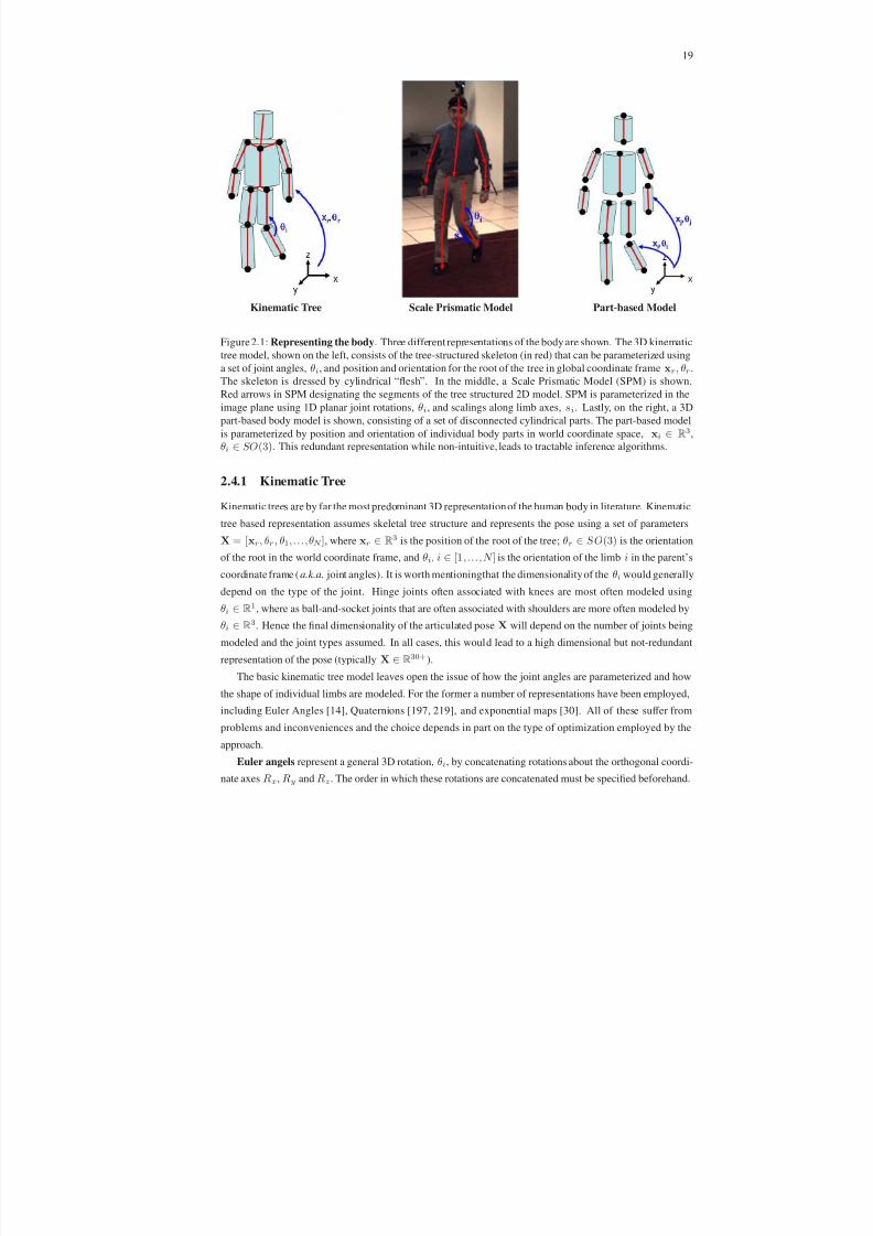
8/13/2019 Continuous-State Graphical Models for Object Localization, Pose Estimation and Tracking
http://slidepdf.com/reader/full/continuous-state-graphical-models-for-object-localization-pose-estimation 34/220
19
Kinematic Tree Scale Prismatic Model Part-based Model
Figure 2.1: Representing the body. Three different representations of the body are shown. The 3D kinematic
tree model, shown on the left, consists of the tree-structured skeleton (in red) that can be parameterized using
a set of joint angles, θi, and position and orientation for the root of the tree in global coordinate framexr, θr.
The skeleton is dressed by cylindrical “flesh”. In the middle, a Scale Prismatic Model (SPM) is shown.
Red arrows in SPM designating the segments of the tree structured 2D model. SPM is parameterized in the
image plane using 1D planar joint rotations, θi, and scalings along limb axes, si. Lastly, on the right, a 3D
part-based body model is shown, consisting of a set of disconnected cylindrical parts. The part-based model
is parameterized by position and orientation of individual body parts in world coordinate space, xi ∈ R3,
θi ∈ SO(3). This redundant representation while non-intuitive, leads to tractable inference algorithms.
2.4.1 Kinematic Tree
Kinematic trees are by far the most predominant 3D representation of the human body in literature. Kinematic
tree based representation assumes skeletal tree structure and represents the pose using a set of parameters
X = [xr, θr , θ1,...,θN ], where xr ∈ R3 is the position of the root of the tree; θr ∈ SO(3) is the orientation
of the root in the world coordinate frame, and θi, i ∈ [1,...,N ] is the orientation of the limb i in the parent’s
coordinate frame (a.k.a. joint angles). It is worth mentioningthat the dimensionality of the θi would generally
depend on the type of the joint. Hinge joints often associated with knees are most often modeled using
θi ∈ R1, where as ball-and-socket joints that are often associated with shoulders are more often modeled by
θi ∈ R3. Hence the final dimensionality of the articulated poseX will depend on the number of joints being
modeled and the joint types assumed. In all cases, this would lead to a high dimensional but not-redundant
representation of the pose (typically X
∈R
30+).
The basic kinematic tree model leaves open the issue of how the joint angles are parameterized and how
the shape of individual limbs are modeled. For the former a number of representations have been employed,
including Euler Angles [14], Quaternions [197, 219], and exponential maps [30]. All of these suffer from
problems and inconveniences and the choice depends in part on the type of optimization employed by the
approach.
Euler angels represent a general 3D rotation, θi, by concatenating rotations about the orthogonal coordi-
nate axes Rx, Ry and Rz . The order in which these rotations are concatenated must be specified beforehand.

8/13/2019 Continuous-State Graphical Models for Object Localization, Pose Estimation and Tracking
http://slidepdf.com/reader/full/continuous-state-graphical-models-for-object-localization-pose-estimation 35/220
20
While this parameterization is intuitive and is often used in biomechanics to study the behavior of joints, it
does suffer from what is called the ‘gimbal lock’ problem. When two out of the three rotation axes align, a
rotation is lost. As a result small changes in an angle can cause large deviation in the orientation of the limb.
This makes this representation very unstable for the use in inverse kinematics and/or direct optimization. For
similar reasons interpolation in the Euler angle space is poorly defined.
Quaternions [191] do not suffer from these problems. However, quaternions are represented as 4D
unit vectors lying on a 3D spherical shell embedded in 4D space, this makes modeling distributions over
quaternions challenging. Using quaternions, a general rotation of angle θ about axis v ∈ R3 can be written as
q = [q x, q y, q z, q w]T = [v ·sin(0.5θ),cos(0.5θ)]. As mentioned, however, valid rotations must maintain that
||q|| = 1. Since there are four dimensions in which quaternion can change but only 3 degrees of freedom,
typical optimization approaches can move away from the unit sphere representing valid rotations. In such
cases the solution is often to re-normalize the quaternion, which works well [197, 219] so long as the distance
from the sphere is small. Quaternions are also well suited for interpolation and are often prefered for that
reason.
Exponential maps [71] is yet another way to model 3D rotations. The idea behind exponential maps is
to try to maintain the benefits of quaternions, while getting a representation ∈ R3. There are many variants
of exponential maps in the literature, however, the basic idea is to model an arbitrary rotation in 3D using a
vector v ∈ R3 such that v/|v| gives the axis of rotation and |v| the amount of rotation. A particular variant
that made this representation popular, in the context of articulated human motion, is twists and exponential
maps formulation of Bregler and Malik [30].
The shape of the person is often modeled using relatively simple 3D geometric representations including
cylinders [180, 193], tapered cones [52, 237], ellipsoids [30], and superquadrics [74, 210, 211]. More com-
plex models such as metaballs [165], mesh-based surface models [215] or free-form surface patches [183]
are also gaining popularity.
2.4.2 Scale Prismatic Model
It is clear that 3D models such as the one described in the previous section cannot be fully observed from a
single monocular image, and hence either temporal or prior knowledge is often required to address ambigu-
ities that arise. In such cases it sometimes may suffice to estimate the pose of the body in the image plane
(not the world) directly. To this end Scale Prismatic Model (SPM) is derived [149] by “projecting” the 3D
kinematic tree model into the image and parameterizing the resulting planar skeleton (stick figure) with as
few parameters as possible. Each 3D joint of kinematic tree in the SPM is replaced by a 2D joint (planar
rotation) with a rotation axis perpendicular to the image plane and scale that accounts for foreshortening ef-
fects due to perspective and out-of-plane rotations. The resulting SPM model often leads to a more compact
representation of the state than a full 3D kinematic tree model. SPM is a 2.5D generalization of “cardboard”
models [111] that have been widely used for 2D articulated tracking.
The planar skeletal structure of SPM also requires a 2D representation for the limbs. In the literature,
rectangles [91], rectangles with rounded corners [132], 2D templates [149], and affine flow patches [111]
have all been used for this purpose.

8/13/2019 Continuous-State Graphical Models for Object Localization, Pose Estimation and Tracking
http://slidepdf.com/reader/full/continuous-state-graphical-models-for-object-localization-pose-estimation 36/220
21
2.4.3 Part-based Representation
While it is natural to represent the body using tree-structured kinematic models such as kinematic trees
or scaled prismatic models, these models tend to require a very high dimensional parameterization where
parameters are correlated in complex ways. This leads to a disadvantage that these models are often compu-
tationally expensive (and often intractable) to deal with, especially for the pose estimation task. To addressthis, it has proven useful to represent the body using a set of disaggregated parts that interact via a set of
pair-wise constraints that attempt to enforce the body consistency. As a result, the body is represented using
a redundant representation in a global space. This representation that leads to an even higher dimensional
parameterization of pose (due to redundancy), decouples many of the parameters, making the search tractable.
The use of disaggregated models for finding or tracking articulated objects date back at least to Fischler
and Elschlager’s pictorial structures [62]. Variations on this type of model have been more recently applied
to general object detection [33, 44, 198], and articulated pose estimation for people [59, 78, 93, 96, 97, 98,
122, 169, 173, 174, 177, 196, 197, 248], animals [170, 172] and hands [219].
Articulated disaggregated models, model the body using simple 2D (e.g. rectangles [59, 122, 169], trape-
zoids [195, 196], quadrangulars [93, 248], polygonal patches [78], or templates [176]) or 3D parts (e.g. right-elliptical cones [197, 199], truncated quadrics [219], or surface models [177]) and set of constraints between
parts that are encoded either directly in terms of compatibility [96, 97, 98, 172, 174] or probabilistically
[59, 78, 93, 122, 169, 196, 197, 248]. Most probabilistic models [59, 122, 169, 174] rely on the underlying
tree-structure of the model for tractable inference and hence are only capable of modeling kinematic con-
straints. In this thesis (and in [195, 196, 197, 198]) we introduce the means of formulating and inferring the
pose using a more diverse set of models that can model any pair-wise relationships between parts statistically.
Kinematic, occlusion and inter-penetration constraints can all be modeled. Recently, similar method has been
introduced for determining the articulated pose of people from range scan data by Rodgers et al. [177].
The pictorial structures approach of Felzenszwalb and Huttenlocher [59] is one of the more influential
2D disaggregated models introduced for articulated pose estimation. The approach models the body parts
using rectangles and the kinematic and joint constraints between parts using Gaussian distributions. The
model assumes that the state of each limb can be discretized and the inference proceeds to find the globally
optimal pose using dynamic programming (that can in this case be interpreted as Belief Propagation, see
Section 3.5.2). This basic model has been successfully extended by introducing richer likelihood functions
[178] or simple dynamics [122]. More recently, the pictorial structures approach has been extended [169] to
elegantly estimate the appearance models of parts jointly with the pose in extended image sequences.
A similar approach to ours has been adopted in [248] for tracking a 2D human silhouette using a dynamic
Markov network and later in [93] using data-driven Belief Propagation. A much simplified observation
model was adopted in [248] and their system does not perform automatic initialization. In [93] a much
richer observation model was used, but the approach is still limited to 2D pose inference in roughly frontal
body orientations; the subject is assumed to be facing towards the camera and wearing distinct clothes.
The [93, 248] and the method proposed in this thesis use somewhat different inference algorithms and a
comparison between these methods merits future research.

8/13/2019 Continuous-State Graphical Models for Object Localization, Pose Estimation and Tracking
http://slidepdf.com/reader/full/continuous-state-graphical-models-for-object-localization-pose-estimation 37/220
22
Synthetic Image Silhouette Edges
Figure 2.2: Common features used for articulated pose and motion estimation. On the left two synthetic
images of a person in different postures are shown; corresponding silhouette features are illustrated in the
middle. Notice that silhouettes in this case are identical and cannot distinguish between the two poses on the
left. Edge features, illustrated on the right, however, clearly contain information required to distinguish the
two poses.
2.5 Image Features
The choice of the model for the body often gives rise to the features that are chosen to match the model to the
image. A typical inference approach proceeds to extract appropriate features from the image and then either
matches these features to features hypothesized by the model, or infers the state of the model directly from
them. While ranking of features that are most useful for the task of articulated pose estimation and tracking
is still debated (relative importance of some feature choices was tested in [14]), it is a general consensus in
the community that combining features leads to better and more robust inference methods. We will describe
some of the more common features used in the literature bellow.
2.5.1 Silhouettes
Silhouettes are among the features most frequently used for two main reasons, (1) they can localize the search
for the body by excluding large portions of the image and (2) they provide features that are easy to compute.
Silhouettes, being region based, are also inherently more robust to clutter then edges or contours. However,
silhouettes are also ambiguous.
Background subtraction is the process often used to obtain the silhouettes. If the scene background
is specifically designed for such a task, as in Chroma-keying [133] where the background is usually blue
or green and is distinct from the clothes worn by the subject, then simple thresholding can be used. An
alternative is to have an arbitrary background but a subject wearing a distinct colored suit [142, 156]. In
both cases very precise silhouettes can be obtained. In more realistic scenarios where the background and
foreground are more general, a statistical representation of the background can be learned either on-line
or off-line. Often a per pixel model of the background is learned and used to classify the image pixels
into foreground and background classes. A sequence of images can be used to learn a per pixel Gaussian
(mean and covariance) and Mahalanobis distance can be used to classify the pixels [247] I shillouette(x, y) =
[(µx,y − I x,y)Σ−1x,y(µx,y − I x,y)T > τ ], where µx,y and Σx,y are mean and covariance of the Gaussian
distribution for background pixel (x, y) learned from training data and τ is the threshold. In the presence
of background motion (e.g. leaves waving in the wind) this approach will lead to poor results. For such
scenarios Gaussian mixture models [216] have been proposed to model multi-modality of background pixel
observations. More sophisticated models that use either color thresholding [86] or pixel gradients [140] to
remove shadows have also been proposed.

8/13/2019 Continuous-State Graphical Models for Object Localization, Pose Estimation and Tracking
http://slidepdf.com/reader/full/continuous-state-graphical-models-for-object-localization-pose-estimation 38/220
23
Since recovered silhouettes are often noisy, due to pixel variations, morphology is commonly used to
‘clean up’ the silhouette image. Alternatively approaches that embed spatial consistency directly into the
background subtraction process have also been proposed [89]. In cases where lighting variations are common
(as in prolonged surveillance applications) background models are often updated on-line to account for global
variations in lighting.
Even with the most sophisticated background subtraction methods often good subtraction is hard to ob-
tain. In particular, often the background colors appear in the foreground (or vise versa), the shadows are hard
to discount completely, and motion in the background creates challenges. Furthermore if multiple foreground
objects are present the assignment of foreground region(s) to objects must be addressed.
2.5.2 Color
Background subtraction at best is only capable of separating the foreground object (person) from the back-
ground. There is no explicit assignment of silhouette pixels to model parts and inference methods must be
employed to simultaneously solve for feature assignment (often not explicitly) and the pose. If color (or tex-
ture) of body parts is known, then assignment can be facilitated thus reducing the complexity of the overallinference significantly. However, color information for parts will generally differ from person to person and
between clothing types, hence often this information is unavailable. Methods have, however, been proposed
that attempt to build the color appearance models for parts automatically either by clustering of coherent
spatio-temporal regions [172, 173] or by roughly estimating the pose first using a generic model, learning the
appearance, and then re-estimating the pose based on the learned image and person specific model [169].
A by far more common assumption is that some parts of the body are not covered by clothes [93, 126,
127], in which case skin color can be used as the signature for these parts. Skin-color detection and segmen-
tation has a long standing history in computer vision. Jones and Rehg [106] introduced a relatively simple
parametric probabilistic model for classifying skin pixels. The key step in proposed skin pixel classification
is the computation of p(skin|I x,y) for a given pixel value I x,y at location (x, y) in an image, which is given
by Bayes rule:
p(skin|I x,y) = p(I x,y|skin) p(skin)
p(I x,y|skin) p(skin) + p(I x,y|¬skin) p(¬skin). (2.1)
A simple threshold 0 < τ sk < 1, p(skin|I x,y) > τ sk, can then be used to classify a given pixel in an
image as belonging to a skin class. The exact value τ sk can be derived based on the risk of misclassification.
In this model both p(I x,y|skin) and p(I x,y|¬skin) are modeled using 16 component Gaussian mixtures
learned from 13, 640 hand labeled images; prior is also learned, p(skin) = 1− p(¬skin) = 0.1. The learned
values for means and covariances are listed in [106].
2.5.3 Edges
Edge features, that are based on first spatial derivatives of the image, are often used due to their partial
invariance to viewpoint, lighting and local contrast. Edges are also capable of discriminating variations in
pose that may be ambiguous by looking at silhouettes ( e.g. they can account for internal structure); this is
illustrated in Figure 2.2. Edges, however, are still limited in that they are insensitive to the rotations of the
limbs around their axis of symmetry (i.e. twists are unobservable).

8/13/2019 Continuous-State Graphical Models for Object Localization, Pose Estimation and Tracking
http://slidepdf.com/reader/full/continuous-state-graphical-models-for-object-localization-pose-estimation 39/220
24
Edges are also very local, comparing a model edge to an image edge that is one pixel away will lead to
nearly zero response. To remedy this edges are often smeared by applying a Gaussian filter over the edge
image [14, 52], as a result the extent of the edge is augmented. Furthermore distance transforms are often
used to define a more global feature space [11] based on edges.
2.5.4 Contours
Contours refer to the edge representation of the object’s full or partial outline. Contours can either be static or
dynamic, where later is often referred to as active contour . Static contours can be thought of as a more com-
pact representation of the silhouette, and inherently carry no more information than silhouettes themselves.
Some invariance to geometry and appearance of the object can be obtained by using contour (or boundary)
fragments that are geometrically constrained [88, 158]. A more general formulation of active contours allows
the contour of the object (either whole or partial) to deform according to the image edges. The deformations
are often controlled by energy functions that consist of two terms: one that attempts to minimize the distance
between the contour and the edges in the image, and the other that controls the overall smoothness of the
curve. The assumption being that in general we want to fit a relatively smooth contour to the image data. Thedeformations of the contour can also embed prior knowledge about allowed deformations for a given object
class, in such cases the model is often referred to as deformable template. Deformable templates have been
successfully applied for pedestrian detection [72] and localization. In general, deformable template models
have lost popularity in recent years. This is partially due to the inherent ambiguities that exist in the contour
representation, and partially due to the fact that while deformations can account to some extent for articu-
lations they are not well suited for recovering those articulations. Contour ambiguities can be circumvented
to some extent by considering contours from multiple calibrated views. Contours from 4 calibrated views
have been used to reliably infer the articulated motion in [182, 184]. More recently, deformable templates
have been used to localize parts of the body (e.g. the head-shoulder outline [126, 127]) as part of a more
sophisticated hierarchical representation of the human body.
2.5.5 Ridges
Ridges refer to the second spatial derivatives of the image at a given scale. Since ridge (or second derivative)
filters account for elongated spatial structure in the image, it has been shown that they are effective in mod-
eling the limbs [192] if applied at a particular scale and orientation that is a function of limb width and pose.
Intuitively ridge features encode the parallel edge structure of limbs in the body. As with any higher deriva-
tive filters ridge filters tend to be noisier then edges alone. They are also highly dependent on the orientation,
configuration, and scale of the person in the image.
2.5.6 Image Flow
Image Flow refers to dense motion information that often is obtained using optical flow algorithms. Image
flow (or optical flow) can be thought of as a vector field in an image that for every pixels defines where that
pixel will move to in the next frame. In general to compute optical flow one must assume that the intensity

8/13/2019 Continuous-State Graphical Models for Object Localization, Pose Estimation and Tracking
http://slidepdf.com/reader/full/continuous-state-graphical-models-for-object-localization-pose-estimation 40/220
25
of the image pixels remains constant over time1 (i.e. no lighting variations) resulting in the following optical
flow constraint:
dI (x,y,t)
dt =
∂I (x,y,t)
∂x
dx
dt +
∂ I (x,y,t)
∂y
dy
dt +
∂ I (x,y,t)
∂t = 0 (2.2)
on the spatio-temporal image signal I (x,y,t). Solving the equation for, [ dxdt , dydt ], results in an optical flow
field (for details see [23]). However, assuming that the motion is independent at every pixel, results in an
underconstrained set of equations. The common solution to this is to assume that the motion is constant over
a neighborhood (a.k.a. spatial coherence assumption). A relatively large neighborhood is needed to constrain
the solution and add some invariance to image noise. Unfortunately in relatively large regions the assumption
of constant motion is likely to be violated due to the differences in depth, lighting and transparencies. As a
result, a size of the region that is reasonable must be picked to leverage the two artefacts. Even so, it is often
observed that foreground motion ‘smears’ onto background, or vice versa, especially in relatively constant
image regions. One alternative that has been proposed to alleviate this, is to assume that there are a known
and relatively small number of consistent motion fields (layers) that make up the overall motion [120, 251]. In
general robust and accurate image flow is challenging and computationally expensive to compute and hence
it is less frequently used for human motion and pose estimation. It is worth mentioning that a simple sparse
temporal motion derivatives computed using frame differencing have been shown to be useful features as well
[235] for general template based object detection.
Optical flow from multiple camera views can be combined to compute scene flow [232]. Just as optical
flow is the two-dimensional motion of points in an image, scene flow is the three-dimensional motion of
points in the world. Scene flow has been successfully used for temporal and view interpolation of human
motion in [231].
2.5.7 Voxels
Just as scene flow is a three-dimensional variant of two-dimensional optical flow, voxel representation is a
three-dimensional alternative to two-dimensional silhouette. Voxel data can be acquired using silhouettes
from multiple cameras [28, 36, 37, 39, 113]. Typically the volume of interest, corresponding to the visible
portion of the scene, is divided into N × N × N equal sized2 voxels [37]. Each voxel is tested if it belongs
to foreground object or background by checking if its projection falls onto silhouette in each camera view.
Voxels that in all camera views project onto the silhouette are labeled as belonging to the object. Voxels
that at least in one of the camera view fall outside the silhouette are automatically labeled as belonging to
background. More recent approaches of Voxel Coloring [36] in addition to silhouette consistency also check
for color consistency across multiple views. Voxel features while powerful, in that they directly provide 3D
information, are very sensitive to noise in silhouettes. To handle this a probabilistic version of voxel based
representation, called probabilistic occupancy grid , was introduced in [65]. Instead of assigning each voxel
a binary label, in [65], each voxel is assigned a probability of belonging to the foreground object. For further
discussion of voxel based methods see Section 2.9.1.
1 Brightness constancy has also been used to formulate likelihood functions directly [192], without explicitly computing the optical
flow.
2 Alternatively, adaptive partitioning is also possible.

8/13/2019 Continuous-State Graphical Models for Object Localization, Pose Estimation and Tracking
http://slidepdf.com/reader/full/continuous-state-graphical-models-for-object-localization-pose-estimation 41/220
26
2.5.8 Image Descriptors
Image descriptors are generic features that have been used in the literature for articulated pose estimation,
image retrieval, image categorization, generic object recognition, and many other applications. There are
many descriptors that exist, that exhibit variety of properties and invariances to geometric transformations. In
this section we will cover the most common descriptors from the recent literature.
Haar Wavelets
A set of image based filters are constructed that correspond to oriented derivative filters of various sizes and
scales. The response of these filters are considered an over-complete feature representation of the image [144]
(or an image patch). In general only a subset of these features is used to represent an object or an image. For
example, AdaBoost [236], automatically constructs an object detector by selecting a sub-set of features most
useful for classification of a given object class. Haar wavelets and AdaBoost will be discussed in depth in
Chapter 4.
SIFT descriptor
Scale-invariant feature transform (SIFT) [135] represents scale-normalized image region (obtained using
standard interest point operators3) with the concatenation of gradient orientationhistograms relative to several
rectangular sub-regions. Image gradient direction and magnitude are computed for every pixel in the region.
Histograms of gradient orientation, weighted by gradient magnitude are then computed for a given set of
non-overlapping sub-regions. Orientations in the sub-region are normalized with respect to the orientation of
the center pixel of sub-region and are histogrammed into Θ bins. The SIFT local descriptor is the concatena-
tion of these gradient orientation histograms for all sub-regions. For convenience, often the scale-normalized
image region is broken into 16 sub-regions and 8 orientation histogram bins for each region, resulting in the
overall descriptor of size 128. More recently [46] it has been shown that better performance (in the visualcategorization task) can be achieved by histogramming not the gradients themselves, but the projections of
gradient images onto a set of basis functions learned from training data using PCA.
Shape Context
Shape context [17] is an alternative to the SIFT descriptor, that only works with binary edges (obtained by
thresholding the magnitude of the derivatives). Also, instead of histogramming the edges into a regularly
spaced grid, a log-polar grid is used. The effect of this is that shape context is much more sensitive to local
variations in shape than more global variations. Scale and orientation can be normalized much like in the SIFT
case to achieve orientation and scale invariance. Typically the shape context is computed for a set of points
equidistantly sampled on the contour of the desired object. The set of histograms corresponding to these
points are then considered as the descriptor for the object or the region. The typical setting is to compute the
shape context for about 100 points on the contour and have 5 polar and 12 orientation bins. At this resolution
the final descriptor is a 6, 000 dimensional vector. Since working with a vector of this size is hard, typically
3 In the original SIFT [135] formulation a difference of Gaussians (DoG) approach [135] is used for keypoint selection which is an
approximation for the Laplacian operator [134]. Alternatively, other approaches like determinant of the Hessian (DoH) [16] ca n be
adopted for the same task. Additional interest point operators frequently used in the literature are Harris [79] and Shi-Tomasi [190]
corner detectors.

8/13/2019 Continuous-State Graphical Models for Object Localization, Pose Estimation and Tracking
http://slidepdf.com/reader/full/continuous-state-graphical-models-for-object-localization-pose-estimation 42/220
27
Body Model Image
Features
FeaturesGenerative
Discriminative
Figure 2.3: Generative and discriminative pose estimation and tracking. Illustration of the generative
and discriminative pose estimation and tracking frameworks. In a generative framework, the model is used to
predict a set of features observed in an image. The model parameters, that typically represent articulated pose,
are then optimized such that predicted features match the features observed. In a discriminative framework,
observed image features are used directly to infer the model parameters.
the shape context space is quantized and secondary voting is used to get a much lower dimensional histogram
representation of the object [1, 4, 166] (typically 100D), which as a consequence looses much of the spatial
information encoded in the original 6, 000 dimensional vector.
2.6 Pose Estimation and Tracking
We found it useful for the purposes of taxonomy to classify approaches to human motion into pose estimation,
tracking, or both. While these two notions are slowly converging, there are still useful distinctions between
the approaches that deal with each of these problems. For the purposes of this thesis we define pose estimation
as estimation of an articulated pose from single monocular or multioccular images and tracking as estimating
of the articulated pose in an image sequence, where the pose estimate for the first frame is known. Approaches
that automatically estimate the articulated pose in the first frame and then track it over an extended image
sequence are classified as both pose estimation and tracking using the above definitions.
It is easy to see that pose estimation is an inherently more general and challenging problem, since it
assumes nothing about the placement or configuration of the body. If we can estimate the pose of the body
from a single image robustly we can also solve tracking by simply performing pose estimation at every
frame. Given the state of the art in pose estimation, however, this is still impractical in general. This solution
to tracking is also extremely inefficient since it ignores important temporal correlations between poses. To
this end, the major contribution of tracking approaches is the use of temporal consistency and motion models
to efficiently search for the pose at future frames given the current estimate for the position and configuration
of the body.
2.7 Discriminative and Generative Methods
Discriminative approaches attempt to learn a direct mapping from image features to 3D pose from either a
single image [1, 179, 181, 189, 206] or multiple approximately calibrated views [77]. These approaches tend
to use silhouettes [1, 77, 179, 181] and sometimes edges [205, 206] as image features and learn a probabilistic
mapping in the form of Nearest Neighbor (NN) search [189], regression [1], Baysian mixture of experts [206],
or specialized mappings [179]. These methods tend to be fast and are often reliable so long as the statistics

8/13/2019 Continuous-State Graphical Models for Object Localization, Pose Estimation and Tracking
http://slidepdf.com/reader/full/continuous-state-graphical-models-for-object-localization-pose-estimation 43/220
28
of features at runtime were captured well by the training set. In general, however, these approaches have
two drawbacks: (1) they tend provide a black-box solution that gives little insight into the problem, and
(2) the performance tends to degrade significantly in cluttered scenes where it is difficult or impossible to
extract good features. Generative approaches tend to work better in such cases, since they model the image
generation process explicitly.
Generative approaches to human tracking have a long history in vision. Most of these approaches rely on
a kinematic tree [139] representation of the body in 2D [111], 2.5D [34], or 3D [30, 52, 193, 210]. In such
approaches the pose is defined by a set of parameters representing the global position and orientation of the
root, usually a torso, and the joint angles representing the state of each limb with respect to the neighboring
part higher up in the tree. The inference in these models amounts to generating a number of hypothesis for
the pose, and evaluating the likelihood that a given hypothesis gives rise to the image evidence. Inference
in such models, however, often requires stochastic search for the parameters in a high dimensional, 25-50D,
state-space. The high dimensionality of the resulting state-space has motivated the development of special-
ized stochastic search algorithms [52, 136, 193] that either exploit the highly redundant dynamics of typical
human motions [193], or use partitioned sampling schemes to exploit the tree-structured nature of the model
[136]. These schemes have been effective for tracking people wearing increasingly complex clothing in the
increasingly complex cluttered backgrounds [210]. However, even with efficient inference algorithm, search
in this high dimensional space without initialization that is close to the solution is computationally imprac-
tical. Hence, most of these methods require manual initialization and are hopelessly lost once the tracker
fails. To handle these problems disaggregated generative models have been introduced. Further discussion
of disaggregated models was given in Section 2.4.3. Some disaggregated models [93] (including the ones in-
troduced in this thesis [196, 197]) could be thought of as spanning both discriminative and generative realm,
since they include a discriminative stage to bootstrap the generative inference.
The discriminative and generative methods in the context of graphical models will further be discussed in
Section 3.2.3. It is also worth mentioning that there are current and on-going efforts to combine discriminative
and generative methods [205], that may lead to more robust solutions in the future.
2.8 Optimization Methods
Most human motion and pose estimation approaches propose some sort of optimization method, direct or
probabilistic, to optimize the pose (and/or body model) subject to the image features observed. This section
will give an non-exhaustive overview of the methods employed.
Direct optimization. Direct optimization methods [212, 228] often formulate a continuous objective
function F (Xt, I t), where Xt is the pose of the body at time t and I t is the corresponding observed image,
and then optimize it using some standard optimization technique. Since F (Xt, I t) is highly non-linear andnon-convex there is almost never a guarantee that a global optimum can be reached. However, by iteratively
linearizing F (Xt, I t) and following the gradient with respect to the parameters a local optimum can be
reached. If a good estimate from the previous time step is available, and the pose changes slowly over time,
then initializing the search with the previous pose often leads to a reasonable solution.
8/13/2019 Continuous-State Graphical Models for Object Localization, Pose Estimation and Tracking
http://slidepdf.com/reader/full/continuous-state-graphical-models-for-object-localization-pose-estimation 44/220
29
Probabilistic inference. It is often convenient and natural to formulate tracking and pose estimation as
probabilistic inference. A probabilistic framework has two advantages over the direct optimization meth-
ods: (1) it can encode the confidence of any given articulated interpretation of the image, and ( 2) and more
importantly, it allows one to maintain multi-modal predictions both spatially and over time. Multi-modality
arises naturally in human motion estimation, since the body in different postures can look very similar (if not
identical) in the image. The number of valid interpretations of the image depend significantly on the features
used, imaging conditions and the temporal history. By maintaining a multi-modal pose hypothesis over time,
approaches can often benefit by resolving the ambiguities as more information becomes available.
Let us assume that the pose of the body,Xt, at time t is generated by a dynamic process. In general, for ar-
ticulated motion estimation we are interested in the joint posterior distribution p(X0,X1,...Xt|I 0, I 1,...,I t),
where I i is a (possibly multiocular) sequence of image observations over time i ∈ [0,...,t]. Since dealing
with the joint distribution over many high-dimensional variables is hard approximations are often made that
only infer the marginals of the joint (see further discussion of this in Section 3.5). The marginal equations are
significantly simplified my introducing Markov assumption over the hidden states. The 1-st order Markov
assumption4 states that pose, Xt, at time t depends only on the pose at t
−1. This model is also known as
Hidden Markov Model (HMM) and will be discussed at length in the next chapter.
p(Xt|I 0, I 1, ...,I t) =
X0
X0
· · ·
Xt−1
p(X0,X1, . . .Xt|I 0, I 1,...,I t) dX0 dX1 · · · dXt−1 =
=
Xt−1
p(Xt,Xt−1|I 0, I 1, ...,I t) dXt−1 (2.3)
Using first Bayes’ rule (Eq. 2.4) and then assuming the independence of observations (Eq. 2.5), in particular,
that I t is conditionally independent of [I 0,...,I t−1] givenXt, we can re-writethe above expression as follows,
p(Xt
|I 0, I
1, ...,I
t) =
Xt−1
p(Xt,X
t−1|I 0, I
1, ...,I
t) dX
t−1
=
Xt−1
p(I 0, I 1,...,I t|Xt,Xt−1) p(Xt,Xt−1)
p(I 0, I 1, ...,I t)dXt−1 (2.4)
=
Xt−1
p(I t|Xt,Xt−1) p(I 0, I 1, ...,I t−1|Xt,Xt−1) p(Xt,Xt−1)
p(I t) p(I 0, I 1,...,I t−1)dXt−1 (2.5)
Since the observation, I t, at time t is assumed conditionally independent of all hidden states (past or
future) given the state, Xt at time t, we can further simplify Eq. 2.5 to Eq. 2.6. Then using conditional
probability rules (Eq. 2.7), re-arranging terms (Eq. 2.8) and applying Bayes’ rule again to the right-most term
(Eq. 2.9) obtain the final recursive expression for Baysian filtering (Eq. 2.10),
p(Xt|I 0, I 1, ...,I t) Posterior at time t
=
Xt−1
p(I t|Xt,Xt−1) p(I 0, I 1, ...,I t−1|Xt,Xt−1) p(Xt,Xt−1)
p(I t) p(I 0, I 1,...,I t−1)dXt−1
=
Xt−1
p(I t|Xt) p(I 0, I 1, ...,I t−1|Xt−1) p(Xt,Xt−1)
p(I t) p(I 0, I 1,...,I t−1)dXt−1 (2.6)
4 Similar expressions can be derived for higher order Markovassumptions, where an n-th order Markov assumption refers to the fact
that the state Xt is assumedto depend on the history of [Xt−n, ...,Xt−1] states.

8/13/2019 Continuous-State Graphical Models for Object Localization, Pose Estimation and Tracking
http://slidepdf.com/reader/full/continuous-state-graphical-models-for-object-localization-pose-estimation 45/220
30
=
Xt−1
p(I t|Xt) p(I 0, I 1, ...,I t−1|Xt−1) p(Xt|Xt−1) p(Xt−1)
p(I t) p(I 0, I 1, ...,I t−1)dXt−1 (2.7)
=
Xt−1
p(I t|Xt)
p(I t) p(Xt|Xt−1)
p(I 0, I 1,..., I t−1|Xt−1) p(Xt−1)
p(I 0, I 1, ...,I t−1)dXt−1 (2.8)
= Xt−1
p(I t|Xt)
p(I t)
p(Xt|Xt−1) p(Xt−1|I 0, I 1, ...,I t−1) dXt−1 (2.9)
=
Xt−1
1
Z p(I t|Xt) p(Xt|Xt−1) p(Xt−1|I 0, I 1, ...,I t−1) dXt−1
= 1
Z p(I t|Xt) Likelihood
Xt−1
p(Xt|Xt−1) TemporalPrior
p(Xt−1|I 0, I 1,...,I t−1) Posterior at time t− 1
dXt−1, (2.10)
where Z is a normalizing constant. The integral portion of the above equation is referred to as the prediction
and the term before the integral, p(I t|Xt), as the likelihood . Furthermore, the first term in the integral, is
also known as the temporal prior that defines the dynamics or the state evolution process. It is worth noting
that the above recursion terminates at p(X0|I 0) = p(X0), where it is assumed that the distribution over the
initial starting poseX0 is known. In the case of the pose estimation p(X0
|I 0)
= p(X0) and itself needs to be
inferred.
If the likelihood is Gaussian, p(I t|Xt) = N (I t; AoXt, Σo), the initial distribution, p(X0), is Gaussian
and temporal prior is linear with normally distributed noise, p(Xt|Xt−1) = N (Xt; AdXt−1, Σd), the inte-
gral in Eq. 2.10 can be dealt with analytically. This model is commonly called the Kalman Filter and has
been used successfully for articulated tracking in some cases [112]. While the Kalman filter provides a prob-
abilistic solution to tracking, this model is only capable of dealing with uni-modal Gaussian predictions of
the posterior. Hence, most state of the art probabilistic methods tend to avoid Kalman Filtering in favor of
other models that make weaker assumptions on dynamics and observations (e.g. particle filtering).
It is worth mentioning that there is significant evidence that the posterior over pose is indeed non-Gaussian
and is hard to model using simple parametric distributions. This arises due to non-linear dynamics of thehuman body and an often non-Gaussian observation model. For example, when a leg hits the ground during
the walking cycle, the result is an inelastic collision between the foot and the ground plane that is highly
non-linear. In terms of observations, based on simple geometry, we know that mapping between the 3D pose
and the 2D pose (which is the only thing that we can observe in the image) is not one-to-one. This means
that naturally an observed image would give rise to multiple hypothesis for the 3D pose 5. Lastly, since body
joints move over large ranges but have hard limits, they are not well modeled using Gaussian or other simple
distributions.
Constructing models that encode these more realistic phenomena, leads to the forms of the integral in
Eq. 2.10 that cannot be dealt with analytically. In such cases a common solution is to approximate the
integral using numerical (e.g. Monte Carlo) integration. This leads to a family of methods that are commonlyknown as Particle Filters. Particle filters will be covered in more detail in Section 3.6.4. Particle filters have
been extensively used for both rigid [157] and articulated object [52, 193] tracking. Unlike the Kalman Filter,
Particle Filters are able to deal with complex and multimodal posterior distributions. Particle Filters tend
to represent the posterior at time t using a weighted set of N samples (particles) s(i)t , w
(i)t |i ∈ [1,...,N ],
where s(i)t is an i-th sample and w
(i)t is the corresponding weight, such that
N i=1 w
(i)t = 1. The most
5 This ambiguity can be significantly reduced by using multiocular observations.

8/13/2019 Continuous-State Graphical Models for Object Localization, Pose Estimation and Tracking
http://slidepdf.com/reader/full/continuous-state-graphical-models-for-object-localization-pose-estimation 46/220
31
notable disadvantage of these methods is that they require sampling in high-dimensional spaces to represent
the posterior. Since the number of samples required growsexponentially with the dimensionality, (a.k.a. curse
of dimensionality), most methods rely on some heuristic function that designates the most plausible portion
of the space to sample. Consequently, the efficency of particle filters is greatly effected by the choice of this
function.
Annealed Particle Filters (APF) [52]. Due to the high-dimensionalityof the state space and often highly
non-convex likelihood function with narrow peaks, the number of samples required to model the posterior in
the realistic cases is intractably high. The Annealed Particle Filter tries to battle this problem using the con-
cept of simulated annealing initially introduced by Kirkpatrick et al. in [116]. Instead of sampling the poste-
rior p(Xt|I 0, I 1,...,I t) directly a series of distributions with probabilitydensities p0(Xt), p1(Xt),...,pM (Xt)
are introduced (also referred to in the context of APF as layers), where pm(Xt) differs only slightly from
pm+1(Xt). These distributions are constructed such that p0(Xt) = p(Xt|I 0, I 1,...,I t), and each subsequent
distribution pm+1(Xt) is designed such that the Markov Chain used to sample from it allows easier movement
between regions of the state/search space. The last layer corresponding to pM (Xt) allows movement between
all regions of the state/search space. The usual method of achieving this is by setting pm(Xt)
∝ p0(Xt)
βm ,
where β m is the temperature parameter such that 1 = β 0 > β 1 > ... > β M . As a result the effect of the
peaks in the posterior is introduced gradually by adjusting the temperature of the posterior distribution.
APF draws samples from the posterior by first simulating the Markov Chain corresponding to the distribu-
tion pM (Xt), then using the resulting estimates of the distribution as initialization for simulating the Markov
Chain corresponding to pM −1(Xt) and so on until Markov Chain corresponding to the desired distribution
(posterior) p0(Xt) is simulated. The proposed method is a heuristic for avoiding local minima and handling
narrow peaks that can be problematic when simulating the Markov Chain corresponding to the posterior
p0(Xt) = p(Xt|I 0, I 1,...,I t) directly.
Hierarchical Particle Filters [51, 136]. Hierarchical particle filters (a.k.a. partitioned sampling) handle
the problem of high dimensionality of the state-space in a different way. They use search space decomposition
to partition the search space into a number of independent searches. If the state space can be partitioned into
parts that can be searched independently, then the computation time would be reduced significantly. Instead
of complexity exponential in the number of degrees of freedom, we can have a search strategy that is linear in
the number of partitions and exponential in the number of degrees of freedom withina partition. For example,
if we partition our state Xt ∈ Rd into K equal partitions (in most realistic cases the partitions will not be
equal) Xt = [xt,1,xt,2,...,xt,K ]T , where xt,k ∈ Rd/K , then instead of exponential search strategy O(cd)
we can have search strategy that is O(Kcd/K ), where c is a constant.
In the context of human motion and pose estimation, the partitioning often takes the following form: first
find the torso, then given the torso find the head and the upper extremities, then given the upper extremities
find the lower extremities, followed by hands and feet. While this strategy is very efficient it suffers fromone significant disadvantage, it assumes that the parts that are high in the hierarchy can be localized well
(e.g. torso). Depending on the imaging conditions and the exact partitioning strategy this assumptions may or
may not hold. In general a dynamic data-driven strategy for the partitioned sampling would be prefered. The
approach introduced in this thesis that uses graphical models to model the conditional independence between
parts of the search space (that correspond to individual body parts) and uses particle message passing to do
the search, can be viewed in this way - as dynamic iterative hierarchical search that is not committed to the
particular partition strategy. It is worth noting that partitioned sampling can also be combined with annealed

8/13/2019 Continuous-State Graphical Models for Object Localization, Pose Estimation and Tracking
http://slidepdf.com/reader/full/continuous-state-graphical-models-for-object-localization-pose-estimation 47/220
32
particle filtering for further speed and robustness improvements [51].
Rao-blackwellized Particle Filters (RBPF) [153]. Standard Particle Filters assume that the integral in
the Baysian filtering equation cannot be computed analytically, in some cases however integrating analytically
over part of the state space may be easy (e.g. a subset of variables inXt may be Gaussian). Rao-blackwellized
Particle Filters make use of this fact by integrating analytically over the part of the state-space that can be
integrated, and sampling the rest. As a result it can be shown that Rao-blackwalized Particle Filters provide
a better estimate for the posterior distribution. While RBPF inference has been successfully used in various
applications, few approaches have thus far attempted to use it for articulate human motion estimation [104].
Hybrid Methods often attempt to integrate particle filtering with deterministic (gradient) optimization
of the posterior [38, 241]. One such example is Hybrid Monte Carlo (HMC) filter [38], that uses multiple
Markov Chains that use posterior gradients to rapidly explore the state space, yielding fair samples from the
posterior. The resulting approach is claimed to be several thousand times faster then the standard particle
filter. Similarly, covariance scaled sampling [210] combines covariance scaled ‘oversized’ sampling with
local optimization subject to joint and non-self-intersection constraints.
In [211] MCMC sampler is modified to include a potential function that focuses samples on nearby saddle
points based on the local gradient and curvature of the input distribution. This strategy effectively finds
local optima in the high dimensional space of articulated poses. Interpretation trees and inverse kinematic
reasoning can be used to construct sampling schemes that account for long-range structural ambiguities of 3D
human motion [209] observed from a monocular camera. This approach has also been extended in [208] by
introducing variational temporal smoothing that accounts for temporal continuity in persistently multi-modal
posterior.
Multiple Hypothesis Tracking is an alternative to the Particle Filtering. Instead of representing the
posterior distribution over the state explicitly, MHT approaches [34, 131] often formulate the problem of
inference as that of explicitly maintaining a fixed number of hypothesis that correspond to the modes of the
posterior distribution.
2.9 Number of Views
As was discussed in the Section 2.4 the human body can be represented in either 2D or 3D. If the 2D repre-
sentation is chosen then at least conceptually one view (or a single image) of the scene should be sufficient to
infer the pose of visible parts. In the case of the 3D model, it is unclear how well one can expect to predict
the pose from a single view, especially when motion information is unavailable. It is known that multiple
3D poses will result in the same 2D image projection, and as a result most approaches that attempt to solve
this problem from monocular imagery must either rely on prior knowledge of the motion [125] or temporal
information [193, 195, 206, 209] to resolve ambiguities. The problem of 3D pose inference, however, issignificantly simplified when multiple views are available. At least conceptually with sufficient number of
non-degenerate6 views, the body can be fully observed and the pose recovered with little or no prior assump-
tions on the motion.
6 By degenerate views we mean views of the scene that give no additional information. For example, cameras that are very close
together resulting in the nearly the same image, would be considered degenerate. Degeneracy may also depend on the features. For
example, cameras that are located opposite to each other (180 degrees apart) can produce identical silhouettes.

8/13/2019 Continuous-State Graphical Models for Object Localization, Pose Estimation and Tracking
http://slidepdf.com/reader/full/continuous-state-graphical-models-for-object-localization-pose-estimation 48/220
33
2.9.1 Multiocular 3D Inference
Most approaches that deal with multiple views can be classified into the ones that either use the visual hull
explicitly or backproject the 3D model into the image without explicitly reconstructing the volumetric repre-
sentation. In both cases the knowledge of the camera parameters (both intrinsic and extrinsic) is essential to
draw correspondences between information in different cameras.Visual hull. Visual hull based approaches explicitly solve for the association of features from multiple
views, resulting in the approximate 3D bounding geometry of the actual object. It can be shown that as
the number of views increase the visual hull tends to approach the true shape of the object. Most visual
hull approaches [28, 36, 39, 113] rely on a good background subtraction process and silhouettes to define the
generalized silhouette cone that originates at the focal point of the camera and runs through the contour of the
silhouette. The intersection of the cones from differentcameras defines the upper bound on the space occupied
by the object. More recent approaches of Voxel Coloring [36] also check color consistency across multiple
views. The key problem with these approaches is their reliance on nearly perfect background separation.
Noisy silhouettes from even a single camera will result in holes in the 3D volume, significantly corrupting
the representation. To attempt to handle this, a probabilistic occupancy grid approach has bin introduced in[65], where an equivalent of the visual hull can be obtained by taking the isosurface of the density at a given
probability. Once the volume is recovered the tracking of the 3D shape can be performed either by stochastic
meta descent [113] or iterative closest point [151].
Backprojection. Alternatively, approaches [52, 74, 77, 112, 197] have used backprojection of the model
into the image to ease the burden of the low level observation association and the need for nearly perfect
silhouette data. In visual hull approaches, hard decisions are made that may result in the loss of information
early (at the feature level). Errors in that stage propagate. The backprojection methods delay hard decisions
until later, when more information is available (such as the full body model), that may resolve ambiguities
and deal with missing data more effectively. In backprojection methods, the multiple views are handled by
the likelihood function, where independence is often assumed across camera views [52, 197] and the product
over individual view-based likelihoods is taken as an overall measure of pose match.
2.9.2 Monocular 3D Inference
The case of inferring a full 3D pose of the person from single monocular image is the most general case
considered by the community. In general, there have been two categories of approaches for doing this: (1)
discriminative methods that attempt to learn the mapping directly from the image features to 3D pose, or ( 2)
methods that recover the 2D pose first and then attempt to characterize the set of 3D poses that are consistent
with the 2D interpretation. Exemplar and probabilistic mapping methods discussed bellow fall into the first
category; geometric and what we call probabilistic 3D reconstruction methods into the second.
Exemplar Methods
The first class of approaches, that has already been discussed to some extent in Section 2.7, attempts to
encode the appearance of the person using a set of generic features (e.g. shape context codebook entries [1, 4],
histograms of oriented gradients [189], boundary fragments [88], Hu moments of the silhouette [179, 180])
and learn the mapping from these features to the 3D pose representation. One popular method is to collect a

8/13/2019 Continuous-State Graphical Models for Object Localization, Pose Estimation and Tracking
http://slidepdf.com/reader/full/continuous-state-graphical-models-for-object-localization-pose-estimation 49/220
34
large dataset of feature- pose associations and build a database. K -nearest neighbor [87, 166] or approximate
K -nearest neighbor [189] methods can then be used to query the database for the entry that matches closely
the features observed in the image and return the associated pose. In doing this, one must typically choose the
similarity measure that is used to compare the features and an efficient (sub-linear) algorithm for search of
the database. In [189] the similarity measure is recovered automatically based on the similarity relationship
imposed on the training data. Alternatively in [11] the embedding that preserves the similarity is computed
and used for faster query computation. These approaches are effective, but requires a database that spans the
set of all possible poses, people, appearances and lightning conditions. This is often impractical for generic
applications where motion, subject and lighting are unconstrained. Alternatively, a coarser discretization of
this space can be used and a locally linear regression employed to interpolate between the poses [189] to get
a continuous estimate for 3D pose. Even so, this class of approaches provides no probabilistic confidence
measure for the recovered pose, nor can it easily embed any priors over the poses without explicitly changing
the content of the database.
Probabilistic Mapping
Alternative approaches [1, 4, 179, 180, 205, 206] attempt to learn a direct continuous probabilistic mapping
between the features and the 3D pose. The set of feature- pose associations in this case are treated as training
data, based on which a much more compact representation of the relationship between these is recovered. For
example, in [1, 4] a simple ridge regression and relevance vector regression (RVM) is used to characterize this
mapping. While effective in some situations, the approach inherently assumes that the relationship between
the 2D features (silhouettes in this case) and the 3D pose is linear and one-to-one, which in general is not
true. In particular, more then one 3D pose can give rise to the same silhouette features depending on the view
of the camera, orientation of the person and pose. To address this, the approach of [1, 4] was extended to
include the multivalued probabilistic mapping [179, 180, 205, 206], and other features (edges and oriented
gradients) that allow observation of occluding parts of the body [205, 206].
Geometric Methods
One alternative to the exemplar and probabilistic methods discussed was proposed by Taylor et al. in [222],
where an approach was introduced capable of recovering a family of solutions based on pure geometry.
Given the knowledge of the set of keypoints corresponding to joint positions in the image (obtained using a
manual labeling procedure) and the knowledge of the 3D body segment lengths connecting these points, the
approach was able to estimate the 3D configuration(s) of the body consistent with 2D constraints, modulo a
scaling factor. While the originalproposed method relied on the manually labeled set of keypoints, it was later
extended by [148], to work from a set of automatically obtained keypoints. These keypoints were obtained by
solving for the 2D pose of the person in an image using a bi-partite matching of shape context features [148].
This geometric approach, however, is relatively unstable with respect to small perturbations of the keypoint
locations in 2D.
Probabilistic 3D Reconstruction
Based on the intuitive notion of using 2D pose to constrain the search for plausible 3D poses, Howe et al. in
[90] proposed the approach that modeled the joint density of the 2D and 3D spatio-temporal poses defined

8/13/2019 Continuous-State Graphical Models for Object Localization, Pose Estimation and Tracking
http://slidepdf.com/reader/full/continuous-state-graphical-models-for-object-localization-pose-estimation 50/220
35
for a fixed size (11 frame) snippet of video. This joint Gaussian Mixture model learned using EM was
then used to derive a conditional distribution of the 3D pose snippet conditioned on the observed 2D pose
sequence. The overlapping 3D motion snippets were then merged using a weighted interpolation resulting in
the continuous motion. While this spatio-temporal model helped to resolve some of the instabilities due to
the jitter of joint positions in a single image, it still relied on the manual initialization at the first frame for
2D tracking, falling short of a fully automatic system. Similar in spirit, an approach was introduced by Brand
in [29], where silhouette moments defined over a motion sequence were used to reconstruct 3D pose. More
recently, there have been attempts to reconstruct the 3D pose from a monocular image, using intermediate
2D pose estimates; an approach taken in Chapter 6 of this thesis. In [127] for example, MCMC sampling
was used to search for the 3D pose that is consistent with 2D probabilistic observations derived from a single
image, based on automatic canonical detection of body parts.
2.9.3 Sub-space Methods
So far we have talked about approaches for monocular 3D pose estimation that are relatively general and
assume little about the nature of the motion itself. Making assumptions about the motion, however, signifi-cantly simplifies the problem in many cases. In particular many simple repetitive motions can be represented
by low-dimensional manifolds in a much higher dimensional space of all possible human motions. This is
the key assumption of the sub-space methods. For example, the walking motion of a known subject can be
parameterized by two parameters: phase and speed [55, 160]. Only one additional dimension is necessary to
capture additional variations across the view of the person [125]. Variations across multiple walking people
have been shown to be captured well in the 3 dimensional non-linear sub-space obtained using Gaussian
Processes Latent Variable Models (GPLVM) [227]. GPLVM has a convenient probabilistic form that defines
bi-directional mapping from and to the latent space. Furthermore, the latent space can be optimized to pre-
serve dynamics [226], resulting in the model where pose estimation and tracking can all be performed in the
latent space significantly reducing the computation required from the search in Rd where typically d = 30+,
to search in R3. A similar approach that uses a Mixture of Factor analyzers for non-linear manifold learning
was introduced by Li et al.[131]. There is, however, an inherent limitation in these models in that the motions
must be relatively simple and/or cyclic. At the moment it is unclear how these approaches can be extended to
work in more general settings where motions are of varying content and complexity.
2.10 Quantitative Evaluation
A variety of statistical [3, 4, 14, 52, 93, 196, 197, 206] as well as deterministic methods [147, 189, 222]
have been developed for tracking people from single [3, 4, 59, 93, 122, 146, 147, 170, 173, 174, 178, 196] as
well as multiple [14, 52, 77, 197] views. All these methods make different choices regarding the state space
representation of the human body and the image observations required to infer this state from the image data.
Despite clear advances in the field, evaluation of these methods remains mostly heuristic and qualitative. As
a result, it is difficult to evaluate the current state of the art with any certainty or even to compare different
methods with any rigor.
Quantitative evaluation of human pose estimation and tracking is currently limited due to the lack of
common “ground truth” datasets with which to test and compare algorithms. Instead qualitative tests are

8/13/2019 Continuous-State Graphical Models for Object Localization, Pose Estimation and Tracking
http://slidepdf.com/reader/full/continuous-state-graphical-models-for-object-localization-pose-estimation 51/220
36
widely used and evaluation often relies on visual inspection of results. This is usually achieved by projecting
the estimated 3D body pose into the image (or set of images) and visually assessing how well the estimates
explain the image [52, 59, 174]. Another form of inspection involves applying the estimated motion to a
virtual character to see if the movements appear natural [206]. The lack of the quantitative experimentation
at least in part can be attributed to the difficulty of obtaining 3D ground truth data that specifies the true pose
of the body observed in video data.
To obtain some form of ground truth, previous approaches have resorted to custom action-specific schemes
(or tricks); e.g. motion of the arm along the circular plate of known diameter [112]. Alternatively synthetic
data has been extensively used [3, 4, 77, 189, 206] for quantitative evaluation. With packages such as POSER
(e frontier , Scotts Valley, CA), semi-realistic images of humans can be rendered and used for evaluation. Such
images, however, typically lack realistic camera noise, often contain very simple backgrounds and provide
simplified types of clothing. While synthetic data allows quantitative evaluation (3D pose is known), current
datasets are still too simplistic to capture the complexities of natural images of people and scenes.
For 2D human pose/motion estimation, quantitative evaluation is more common and typically uses hand
labeled data [93, 170, 173]. While quantitative evaluation does occur, the datasets are typically unique to
each research group, preventing direct comparison of methods. Furthermore, for both 2D and 3D methods,
no standard error metrics exist and results are reported in a variety of ways which prevent direct comparison;
e.g. average root-mean-squared (RMS) angular error, silhouette overlap, joint center distance, etc.
One of the contributions of this thesis is the new dataset, that we call HUMANEVA, that contains large
amount of synchronized motion capture and multi-camera video data. A number of subjects were captured
using the specialized setup performing a set of predefined actions in regular clothing. As part of this effort, we
also outline a set of metrics for measuring error, that in our view make it easier to compare various methods
on equal footing. The details of the dataset and the metrics will be discussed in Section 5.7.1; the data can be
obtained from http://vision.cs.brown.edu/humaneva/.
2.11 Generic Object Detection, Localization and Categorization
Thus far we have concentrate on the articulated object pose estimation and tracking, however, the approaches
introduced can be generalized to work for generic object detection tasks. We briefly cover the three major
classes of approaches for generic object detection, localization and categorization bellow.
2.11.1 Sliding Window Classifiers
Sliding window classifiers refer to the class of approaches that attempt to encode the appearance of the
object as a whole and then classify the patches in the images as either conforming to the object model or
not. The classifier is typically learned from a fixed size registered set of image templates. To find objects at
different positions, scales and rotations in the image typically the image itself is transformed to a fixed set
of canonical scales and orientations and the classifier is slid (hence the name) across this set of constructed
images. Typically the classifier will not respond only at a single location and scale where an object is present,
but rather will respond in the neighborhood producing a family of hypothesis. To resolve this the standard
approach is to apply non-maximal suppression, and report only the results that correspond to the set of local
maxima. Note that although the classifiers are learned, the non-maximal suppression procedure is typically

8/13/2019 Continuous-State Graphical Models for Object Localization, Pose Estimation and Tracking
http://slidepdf.com/reader/full/continuous-state-graphical-models-for-object-localization-pose-estimation 52/220
37
designed by hand.
One of the prime examples of the sliding window classifier is AdaBoost introduced by Viola and Jones
[236]. A cascade of classifiers is learned based on Haar Wavelets that were discussed in Section 2.5.8.
The cascade allows fast classification, by quickly rejecting regions that are unlike the object (regions of
constant color or texture) and spending more time resolving harder ambiguous cases. The approach can also
be amended to deal gracefully with detection of multiple objects, by choosing features that are common
to multiple classes of objects (but still discriminative) for classification [223]. An alternative is to use a
support vector machine (SVM) classifier based on either Haar wavelets [144] or PCA based features [124].
One important challenge for these methods is appearance changes that result from both the viewpoint of the
object and the variations within an object class. Typically only minor variations in both can be accounted for
by these classifiers.
2.11.2 Part-based Models
A number of authors in recent literature [59, 144, 249] suggested that modeling complex objects by compo-
nents explicitly and then combining [59, 144] or statistically fusing [93, 249] the information is superior tothe global appearance approaches (that model variations in parts implicitly) in the presence of partial occlu-
sions, out-of-plane rotation and/or local lighting variations. Component-based detection is also capable of
handling highly articulated objects, for which a single appearance model may be hard to learn. To this end,
it is common to represent objects as collections of features with distinctive appearance, spatial extent, and
position [33, 61, 144, 235, 236, 243]. There is, however, a large variation in how many features one must
use and how these features are detected and represented. There are also variations in how much geometry is
encoded in the model. Typically part based approaches detect a set of interest points or keywords, based on
which local (often scale and/or rotation invariant) image descriptors are derived. The object models are then
learned based on these descriptors in supervised [198, 236], semi-supervised [61] or non-supervised [204]
fashion.
The simplest model in this category is the bag of words model [45, 58, 204] that originated in the doc-
ument analysis community [84]. The key idea is that any object can be represented using a codebook of
visual descriptors/codewords. In this model the spatial relationships between the parts are ignored and only
the presence/absence of the codewords is encoded using a histogram based representation. As a result these
approaches tend to be very useful in image categorization, where one only needs to reason about the object
presence. They are not able to infer the position, rotation or configuration of the object in the image however.
The constellation model is a very influential model for object class detection that was introduced by
Weber et al. [243] and later extended by Fergus et al. [61]. This is a generative model defined over interest
point locations and appearances. Unlike the “bag of words” model, the constellation model strongly param-
eterizes the geometric relationships of parts using a joint Gaussian over both centroid positions of all parts
and individual appearances of parts themselves. Assuming that we have a set of N parts in an object and the
appearance of each part is encoded using a 128 dimensional SIFT [135] vector, we can express the model as
a Gaussian in R128N . Since this model has a simple Gaussian form the probability of a set of N keypoints
can easily be evaluated, however, we must search over all possible assignment of M descriptors found in the
test image to N parts encoded in the model. Hence the complexity of performing localization of a single
object is O(M N ), where M is typically around 100 − 500. This exponential complexity in the number of

8/13/2019 Continuous-State Graphical Models for Object Localization, Pose Estimation and Tracking
http://slidepdf.com/reader/full/continuous-state-graphical-models-for-object-localization-pose-estimation 53/220
38
parts ensures that this model is only tractable for objects that can be encoded using small number of parts
(N ≈ 5). The model also cannot easily handle clutter or occlusions. A recent extension to this model called
a common frame model [145] encodes the position of parts relative to the centroid of the object, leading to a
more efficient inference algorithm.
The pictorial structures model [59] that was discussed in the context of disaggregated models for human
pose and motion in Section 2.4.3 encodes a looser pair-wise geometric relationships between parts, allowing
efficient inference of the configuration along with the position and orientation. Unlike the “constellation
model”, the detection and localization can be done in the time linear in the number of parts. Similar models
have also been introduced by Agarwal et al. [5], Amores et al.[7] and Opelt et al.[158]. These approaches
differ significantly in the features used to encode the appearance and in the specifics of the model, however,
the common underlying premise is to model both appearance and pair-wise geometric constraints on the parts.
2.11.3 Hierarchical Composition Models
Part-based models deal well with deformable and articulate objects, but also tend to be relatively slow (apart
from the “bag of words” model that is not able to perform localization). To be able to deal with deformablestructure faster, a new class of methods has recently started to emerge. This relatively novel class of models
attempts to model compositionality of objects in terms of parts. This compositionality is most often encoded
by a hierarchical model. In this model the root of the hierarchy corresponds to a full model of the object
with all it’s intricacies, and the lower-levels to simpler features that are easier and faster to detect. This
hierarchical structure facilitates rapid object detection and inference. In [263] a shape based hierarchy is
defined and encoded using a statistical graphical model. The inference in this model can be done efficiently
using Belief Propagation (BP), resulting in the reported performance that is 100 times faster then competitors.
Athitsos et al.[10] introduced a very flexible approach that uses grammar like syntax to detect and localize
deformable objects that can have variable structure (i.e. varying number of sub-parts). One example of such
a class of objects is branches with leaves. The approach is an extention of Hidden Markov Models (HMMs),
often used for analysis of temporal data, that in this case is adapted to modeling of the variable deformable
spatial structure of an object. In a similar attempt, probabilistic grammars have also been used by Zhu
et al. [262] to model and detect objects.
8/13/2019 Continuous-State Graphical Models for Object Localization, Pose Estimation and Tracking
http://slidepdf.com/reader/full/continuous-state-graphical-models-for-object-localization-pose-estimation 54/220
CHAPTER 3
Graphical Models and Inference
Graphical models have a wide applicability in statistics, machine learning, statistical physics, and more re-
cently computer vision. Graphical models capture the way a joint distribution over all random variables can
be decomposed into a product of factors each depending on only a subset of variables. This local decompo-
sition of the joint distribution often leads to tractable inference algorithms. Graphical models also provide
simple and intuitive way to visualize the structure of probabilistic models.
A probabilistic graphical model in general can be encoded using a graph G = V , E that comprises of
a set of nodes or vertices, V , and a set of edges, E . Each vertex, i ∈ V , in this graph is associated with a
random variable Xi. These variables can either be continuous or discrete depending on the problem. Each
edge (i, j) ∈ E can be thought of as a probabilistic relationship between random variables associated with
pair of distinct nodes i ∈ V and j ∈ V . It is often useful to partition vertices, V , in a graphical model into
two disjoint sets, V = V X, V Y, where the second set V Y, corresponds to the nodes in the graph that are
associated with variables Y = Yi|i ∈ [1,...,M ] (where M = |V Y |) that are directly observed, and the
first set V X corresponds to the nodes in the graph that correspond to variables X = Xi|i ∈ [1,...,N ](where N = |V X|), that are not observed directly but the value of which is of some interest. It is notationally
convinient to shade the nodes ∈ V Y gray, to make it visually clear that they can be observed.
Graphical models in general can be categorized into three categories: directed, undirected, and factor
graphs. Directed models, also called Baysian Networks (BN), are useful for expressing causal relationships.
If the graph is directed then the edges, that are often depicted using arrows, correspond to the conditional
dependencies of the child nodes (nodes toward which the arrows are pointing) on the parents (nodes from
which the arrows originate). Undirected models, also known as Markov Random Fields (MRF), are used to
encode constraints or correlations between random variables. In undirected graphical models the edges are
depicted using arrow-less lines between nodes. Factor graphs are a relatively recent addition to the graphical
model family, that generalizes both directed and undirected models. A factor graph is defined as an undirectedbipartite graph G = V , F , E, where V and E are defined as before, and F is the set of additional vertices
that are called factors.
Graphical models themselves only encode the structure of the joint distribution using a graph G = V , E(or G = V , F , E in the case of the factor graph), the specific forms of the relationships between random
variables in the graph are not specified explicitly. Hence, in addition to specifying the graphical model, one
must also specify the parameters of the graphical model, θ, where the form of these parameters will depend
39

8/13/2019 Continuous-State Graphical Models for Object Localization, Pose Estimation and Tracking
http://slidepdf.com/reader/full/continuous-state-graphical-models-for-object-localization-pose-estimation 55/220
40
X1
X2 X3
X4 X5
X1
X2 X3
X4 X5
X1
X2 X3
X4 X5
Bayesian Network Markov Random Field Factor Graph
Figure 3.1: Graphical model families. Three families of graphical models that will be discussed
in this chapter are illustrated. All three graphs can encode the same underlying joint distribution,
p(X1,X2,X3,X4,X5), given the proper choice of parameters. Different choices of parameters would lead
to different encoded joint distributions.
on the problem and the parameterization chosen for the variables and their relationships.
While graphical models define a rich set of models, there are only a few canonical operations that one is
often interested in performing using these models. In particular, (1) learning of model structure, (2) learningof model parameters given the structure of the model, and ( 3) inference using the model where both structure
and the parameters are known. The first task is by far most complex and deals with estimating the nodes,
V , in the graph and the connections between nodes, E , corresponding to the relationship between random
variables. In general to be able to do useful structure learning one typically must assume sparseness priors
on both the edges and the nodes, attempting to recover the graph with as few nodes and edges as possible
subject to the observed data. We will not address structure learning ( a.k.a. model selection) in this thesis, and
refer readers to [12, 129, 200, 201] for some recent work in this area. Parameter learning refers to estimating
parameters θ given the model structure G = V , E and subject to the data observed. We will cover a few
examples of this in Section 3.4. The last task of inference is central to this thesis and will be covered in depth
in this chapter. Inference in the graphical model, typically refers to finding the value, or the distribution overthe values of all or some sub-set of hidden variables given the observations. Consequently parameter learning
can often be cast as an inference problem itself.
In the following sections we introduce and compare several different classes of graphical models, includ-
ing directed, undirected and factor graphs. We also introduce some specific instances of models within each
class that are both common and useful for the purposes of this thesis. We also introduce methods for learning
parameters and doing inference in these models.
3.1 Graphical Model Building Blocks
In this section we will introduce the set of distributions commonly refereed to in this thesis and their prop-
erties. These distributions will play a key role in constructing more complex models used throughout this
thesis, and in doing inference in these models.
3.1.1 Exponential Family
The exponential family of distributions is a class of distributions that serve as building blocks in graphical
models, and give rise to rich probabilistic models used throughout the thesis. The distribution p(X|θ), where

8/13/2019 Continuous-State Graphical Models for Object Localization, Pose Estimation and Tracking
http://slidepdf.com/reader/full/continuous-state-graphical-models-for-object-localization-pose-estimation 56/220
41
X is a random variable and θ is a set of parameters, is said to be part of the exponential family if it can be
written in the following form:
p(X|θ) = 1
Z (θ)h(X)exp
θT t(X)
(3.1)
where,
θ is a vector of parameters (a.k.a. natural or canonical parameters)
t(X) is a function referred to as sufficient statistics
Z (θ) is a normalizing constant (a.k.a. partition function) defined as
Z (θ) =
h(X)exp
θT t(X)
dX for continuous variable X, and
Z (θ) = X
h(X)exp
θT t(X)
for descrete choice of X
h(X) is a function of X.
Many distributions can be written in this form, including Bernoulli, Poisson, Gaussian, Beta and Gamma
densities. While the exponential family has many convenient properties, one that is worth mentioning is that
the joint probability of N i.i.d. samples from the distribution, D = xi ∼ p(X|θ)|i ∈ [1,...,N ], can bewritten in the following form,
p(D|θ) = p(x1,...,xN |θ) =N i=1
p(xi|θ)
=N i=1
1Z (θ) h(xi)exp
θT t(xi)
=
N i=1
1Z (θ) h(xi)
exp
θT
N i=1
t(xi)
,
(3.2)
which suggests that the dimensionality of the sufficient statistic remains the same with the number of samples.
This, in turn means that in order to characterize a distribution in the exponential family, it is sufficient to
compute the sufficient statistics. Once we have sufficient statistics for the distribution the samples themselvesgive no additional information about the distribution that generated them. This gives a convienient compact
form for representing distributions in this family. For the list of other common properties of exponential
family we refer the reader to [22, 107].
3.1.2 Gaussian Distribution and Properties
In this section we will review a Gaussian (or Normal) distribution, which is a prime example of the exponen-
tial family. A univariate Gaussian distribution with mean µ and variance σ2 on random variable X ∈ R can
be written as,
p(X|µ, Σ) = 1σ√
2πexp
−12
(X − µ)2
σ2
. (3.3)
Alternatively we can also introduce the shorthand notation N (X|µ, Σ) or N (X; µ, Σ). It is easy to see that a
univariate Gaussian is an exponential family distribution with the following parameterization,
θ =
µ/2σ2
−1/2σ2
, t(X) =
X
X2
, Z (θ) = exp
µ2σ2 + log σ
, h(X) = 1
2√
2π. (3.4)

8/13/2019 Continuous-State Graphical Models for Object Localization, Pose Estimation and Tracking
http://slidepdf.com/reader/full/continuous-state-graphical-models-for-object-localization-pose-estimation 57/220
42
If X is multivariate random variable, X ∈ Rd, then the distribution can be written in the more general
form,
p(X|µ, Σ) = 1
(2π)d/2|Σ|1/2 exp
−1
2(X − µ)T Σ−1(X− µ)
, (3.5)
where Σ is now a covariance matrix and µ a multivariate mean. The Gaussian distribution has a number of convienient properties that make it very useful for modelling and inference tasks. The two most important
properties that relate to the product of Gaussian distributions and conditional distribution of jointly Gaussian
variables are stated bellow.
Product of Gaussian distributions
Product of two or more Gaussian distributions is also a Gaussian distribution. For example, product of M
Gaussian distributions p(Xi) = N (Xi|µi, Σi), i ∈ [1,...,M ] is
p(Y) =M
i=1
p(Xi) =
N (Y
|µY, ΣY), (3.6)
where
ΣY =
M i=1
Σ−1i
−1
µY = ΣY
M i=1
Σ−1i µi
. (3.7)
Conditional Gaussian distribution
A conditional distribution of two or more jointly Gaussian variables is also a Gaussian [22, 217]. Consider a
case of two jointly Gaussian variables X and Y,
N XY
| µX
µY
, ΣX ΣXY
ΣYX ΣY
. (3.8)
We can write conditional distribution p(X|Y) as a normal distribution with the following parameters for
mean and covariance respectively:
µX|Y = ΣXYΣ−1Y
(Y − µY) (3.9)
ΣX|Y = ΣX − ΣXYΣ−1Y
ΣXY. (3.10)
3.2 Bayesian Networks
Baysian Networks is a family of graphical models that characterize how the joint distribution over a set of N
variables, p(X1,X2,...,XN ), factors into a set of conditional relationships imposed by the structure of the
graph G = V , E. By the product rule, it can be shown that the joint distribution defined by the graph can be
written as the product of conditional distributions for each node, where the variable associated with the node
is conditioned on all the parents of that node in the graph. Hence, for a general directed graph with N = |V|variables, the joint distribution can be written as:

8/13/2019 Continuous-State Graphical Models for Object Localization, Pose Estimation and Tracking
http://slidepdf.com/reader/full/continuous-state-graphical-models-for-object-localization-pose-estimation 58/220
43
X1
X2 X3
X4 X5
Conditional Independence Constraints
(imposed by the graph structure)
X1 ⊥⊥ X2,X3,X4,X5X2 ⊥⊥ X3,X4,X5X3 ⊥⊥ X2,X4,X5X4 ⊥⊥ X1|X2,X3, X4 ⊥⊥ X5X5 ⊥⊥ X1|X3, X5 ⊥⊥ X2,X4
p(X) = p(X1,X2,X3,X4,X5) = p(X5|X3) p(X4|X2,X3) p(X3|X1) p(X2|X1) p(X1)
Figure 3.2: Baysian Networks. Example of baysian network graphical model. The joint distribution factors
into the product of conditional distributions as illustrated above. All the conditional independences imposed
by the graph itself are also listed. Notice that even though there seems to be a loop in the graph, there are no
directed cycles.
X1 X2 X3 X4 X5 X6 X7 X8 X9
Figure 3.3: Markov Chain. Graphical model corresponding to a first-order Markov Chain. First-order
Markov assumption encoded in the model presumes that the state, Xt, at time t is only a function of the state
at t − 1 for all t ∈ [2,...,T ], where in the example above T = 9.
p(X1,X2,...,X|V|) =i∈V
p(Xi|XA(i)), (3.11)
where A(i) ∈ V is defined as a function that returns all parents of the node i ∈ V in a graph; XA(i) is then
the set of associated variables
Xk
|k
∈ A(i)
. The equation above expresses the factorization properties
of the joint distribution and holds for all joint distributions and all definitions of variables Xi, i ∈ V . In
order to ensure that factorization holds, an important restriction on the graph topology must be maintained.
In particular, graph G = V , E cannot contain cycles, (i.e. it must be a directed acyclic graph (DAG)). In
other words, there cannot exist a path from any node in the graph along the directed edges that leads back to
the node itself. Example of the directed graphical model and the factorization of the joint distribution over
all the variables is given in Figure 3.2.
3.2.1 Markov Chains
Markov Chains are among the simplest directed graphical models. A first-order Markov Chain is defined on
a series of random variables X1,X2,...,XN such that the following conditional independence holds for
n ∈ [1,...,N −1]:
p(Xn+1|X1,...,Xn) = p(Xn+1|Xn). (3.12)
This conditional independence can be encoded in the graphical model as is shown on Figure 3.3. The
Markov Chain can then be specified by the initial distribution p(X1) and the conditional distribution for the
subsequent variables (a.k.a. transition probabilities). A Markov Chain is called homogenous if the conditional

8/13/2019 Continuous-State Graphical Models for Object Localization, Pose Estimation and Tracking
http://slidepdf.com/reader/full/continuous-state-graphical-models-for-object-localization-pose-estimation 59/220
44
X1 X2 X3 X4 X5
Y1 Y2 Y3 Y4 Y5
X1 X2 X3 X4 X5
Y1 Y2 Y3 Y4 Y5
(a) (b)
Figure 3.4: Hidden Markov Models. Directed graphical model representation of the temporal Hid-
den Markov Model (HMM) with T = 5 observations and hidden variables are shown. Models that il-
lustrate first-order and second-order Markov dynamics are shown in (a) and (b) respectively. In gen-
eral an N -th order Markov assumption in the directed model above states that the hidden variable Xt
is conditionally independent of all observation past or future given the estimates for Xt−N ,...,Xt−1,
i.e. p(Xt|X \Xt) = p(Xt|Xt−N ,...,Xt−1), where X = X1,X2,...,XT .
distributions are the same for all variables in the model. Marginal probability of a particular variable in the
chain can be computed recursively using the following,
p(Xn+1) = Xn
p(Xn+1|Xn) p(Xn) or p(Xn+1) = Xn
p(Xn+1|Xn) p(Xn) dXn, (3.13)
depending on whether the variables are discrete or continuous respectively. The distribution p(X) is said to
be stationary if the following condition holds,
p(X) = X
p(Xn+1|X) p(X) or p(X) = X
p(Xn+1|X) p(X) dX. (3.14)
Markov Chains are extremely useful for inference of other more complex models as will be shown in
Section 3.6.3. In particular, one can design a Markov Chain in such a way as to facilitate sampling from an
arbitrary complex distribution. To this end another property of Markov Chains must be introduced, ergodicity.
Ergodicity ensures that for a given choice of the stationary distribution p(X), p(Xn) will converge to p(X)
as n → ∞ irrespective of initial choice of distribution p(X1). Such a stationary distribution is also called an
equilibrium distribution. It is worth mentioning that while a Markov Chain may have a number of stationary
distributions, an ergodic Markov Chain will have only one equilibrium distribution.
3.2.2 Hidden Markov Models
One of the most common Baysian Networks is the Hidden Markov Model (HMM). A Hidden Markov Model
is often used to model temporal stochastic processes. The HMM is widely used in speech recognition [168],
natural language processing [35], analysis of biological data [81], and computer vision applications. In
computer vision, HMMs are particularly useful for temporal modeling of object motion over time [14, 51,
52, 157].
In an HMM, as is suggested by the name the nodes in a graph G = V , E are partitioned into two sub-
sets V = V X, V Y, where the first set corresponds to the hidden variables X = X1,X2,...,XT that are
not directly observed and the second to the observations Y = Y1,Y2,...,YT that are generated based
on the hidden states. Furthermore there is an evolution process that is defined on the hidden variables Xt,
t ∈ [1,...,T − 1]. For example, we can assume that the hidden states evolve according stationary first-order

8/13/2019 Continuous-State Graphical Models for Object Localization, Pose Estimation and Tracking
http://slidepdf.com/reader/full/continuous-state-graphical-models-for-object-localization-pose-estimation 60/220
45
X
Y
X1 X2
X3
Y1 Y2
X
Y
X1 X2
X3
Y1 Y2
(a) (b) (c) (d)
Figure 3.5: Generative and discriminative graphical models. A symbolic graphic representation of gener-
ative (a) and discriminative (b) models are shown. A specific instance of the generative and discriminative
model is shown in (b) and (c) respectively.
temporal Markov process as illustrated in Figure 3.4 (a). The joint distribution over all variables can then be
written according to the Baysian Network rules as follows:
p(X,Y) = p(Y1|X1) p(X1)T t=2
p(Yt|Xt) p(Xt|Xt−1). (3.15)
If we further assume that hidden variables are discrete and can assume K states, then the total number of parameters required to encode the model is |θ| = K + K (K − 1), where the prior, p(X1), can be encoded
using K parameters and the conditional, p(Yt|Xt), using a matrix with K (K − 1) parameters (where each
parameter will encode the probability of transitioning from a given state at time t−1 to any other state at time
t). Since the sum of all K transition probabilities from a given state at time t − 1 is 1, there are actually only
K − 1 free parameters. Higher order Markov models are also possible (e.g. a second-order temporal Hidden
Markov Model is illustrated in Figure 3.4 (b)). However, the number of parameters required to encode the
model will grow exponentially with the order of the model. In particular, M -th order HMMs will require
|θ| = K + K M (K − 1) parameters. It is worth mentioning that HMMs can be used to encode spatial as
well as temporal structure. For example, HMMs have been successfully used for deformable shape matching
in [10]. HMMs also do not need to be stationary, in which case the number of parameters will depend
on the length of the chain itself. For a sequence with T observations, an M -th order HMM, will contain
|θ| = K + (T − 1)K M (K − 1) parameters.
The formulation above also holds if variables are continuous. In such cases often a linear-Gaussian
dynamical model is chosen for the conditional p(Xt|Xt−1) = aXt−1 + b, where a corresponds to the
deterministic component and b to the noise that is usually assumed to be zero mean normal b ∼ N (0, Σ).
This is also known in the literature as the autoregressive (AR) dynamical model. Generic and articulated
object tracking in the computer vision literature is often formulated using HMMs with first- or second-order
autoregressive dynamics [24, 51].
3.2.3 Generative and Discriminative Graphical Models
The Hidden Markov Model is a prime example of a Generative Graphical Model. Generative graphical
models refer to the class of models that aim at modeling the process by which the data is generated. They
attempt to estimate the joint distribution over all hidden and observed variables and then manipulate the joint
distribution to compute the desired probability densities (e.g. marginals or conditionals). For example, if one
is interested in inferring the state of hidden variables X = X1,X2,...,XN , as is the case for classifica-
tion, then the joint distribution p(X,Y) can be conditioned on the observations Y = Y1,Y2,...,YM

8/13/2019 Continuous-State Graphical Models for Object Localization, Pose Estimation and Tracking
http://slidepdf.com/reader/full/continuous-state-graphical-models-for-object-localization-pose-estimation 61/220
46
resulting in the desired conditional p(X|Y). Since the joint distribution is often complex and can contain
many variables it is often desirable to constrain the distribution before attempting to estimate it. Conditional
independence constraints encoded in the graphical models are one way of doing this. Alternatively or in
conjunction, one can impose prior distributions over the parameters of the joint distribution or the variables
themselves, such priors are often referred to as hyperpriors. Typically one can impose a hierarchy of such
priors, with the model being less sensitive to the parameters that are higher in the hierarchy.
In general, the generative model can be drawn symbolically in the form of the directed graph in Figure 3.5
(a). The hyper-nodeX in the graph corresponds to all the hidden variables X = X1,X2,...,XN and node
Y = Y1,Y2,...,YM to all observations. The arrow designates that all arrows in the graph are only al-
lowed to point from the hidden variables to the observations and not vice versa (nothing is assumed about the
relationship of hidden variables themselves). To estimate the joint distribution, that is often written according
to directed graphical model rules as, p(X,Y) = p(Y|X) p(X), one needs to estimate the prior p(X) and the
conditional (often referred to as the likelihood ) p(Y|X). Since generative models are flexible and can poten-
tially encode all knowledge about the variables and their relationships, they often have good generalization
properties (i.e. they can deal with data that was not part of the training). In other words, since generative ap-
proaches aim at modeling the data generation process, they can draw inferences about all possible data values.
Unfortunately, building realistic generative models is both hard and computationally expensive, hence, most
approaches only model the most important relationships that result in weak but tractable generative models.
Since in some cases we may be only interested in the prediction of the hidden variable state from the
observed data, there may be no need to estimate the full joint distribution p(X,Y). Instead, discriminative
models attempt to estimate the conditional p(X|Y) directly. Alternatively these models can be thought
of as estimating the direct (and often probabilistic) mapping from the observations to the hidden states.
The directed graphical model depiction of discriminative models can be seen in Figure 3.5 ( c). The major
difference is in the direction of the arrows that now point from the observations to the hidden nodes depicted
by the hyper-nodesX andY. This has significant implications, however, in that discriminative models cannot
model any prior information about the hidden variables; conversely they often encode prior relationships on
the data itself making it hard for the discriminative approaches to generalize.
3.3 Undirected Graphical Models
Undirected graphical models capture correlations or constraints between variables instead of causal (or condi-
tional) relationships encoded by directed graphical models. Undirected graphical models fall into the category
of generative models described in Section 3.2.3.
3.3.1 Markov Random Fields
Markov Random Fields (MRFs) represent a class of graphical models that can be characterized by an undi-
rected graph G = V , E, where the edges, E , imply conditional independence relationships between ran-
dom variables associated with the nodes, V . In particular, for a given node i with associated random vari-
able Xi, let us assume we have a function A(i) ⊂ V that returns all neighbors that are connected to i
by an edge. We can then express V for a given choice of i using three disjoint sets V = i, A(i), B(i),

8/13/2019 Continuous-State Graphical Models for Object Localization, Pose Estimation and Tracking
http://slidepdf.com/reader/full/continuous-state-graphical-models-for-object-localization-pose-estimation 62/220
47
X1
X2 X3
X4 X5
Conditional Independence Constraints
(imposed by the graph structure)
X1 ⊥⊥ X4,X5|X2,X3X2 ⊥⊥ X5|X1,X3,X4X4
⊥⊥ X1,X5
|X2,X3
X5 ⊥⊥ X1,X2,X4|X3
p(X) = 1Z ψ123(X1,X2,X3)ψ234(X2,X3,X4)ψ35(X3,X5)
Figure 3.6: Markov Random Field. Example of an MRF graphical model. The joint distribution factors into
the product of potentials as illustrated above. All the conditional independences imposed by the graph itself
are also listed.
where B(i) = V ∩ i, A(i). The set of random variables associated with A(i) and B(i) can be writ-
ten as follows XA(i) = Xj| j ∈ A(i) and XB(i) = Xj | j ∈ B(i) respectively. The conditional
independence constraints encoded by the graph can then be expressed using the following relationship,
p(Xi,XB(i)|XA(i)) = p(Xi|XA(i)) p(XB(i)|XA(i)) for ∀i ∈ V . In other words, we can say that any vari-
able Xi is conditionally independent , given its neighbors, of all other variables in the model. Conditional
independence is very important in design of efficient inference algorithms for these graphical models.
For MRFs it is useful to define the notion of the clique. A clique, c, is defined as the set of fully connected
nodes in the graph. The random variables associated with a clique can be denoted as Xc = Xi|i ∈ cAccording to the Hammersley and Clifford Theorem (restated here for completeness), the joint distribution
over all variables can be parameterized by a product of potential functionsdefined on the cliques of the graph.
In particular,
p(X) = 1
Z c∈C ψc(Xc), (3.16)
where C is the set of all cliques in a graph G = V , E. It is easy to see that in general the parameterization
using the cliques is not unique. To get a unique parameterization, often maximal cliques are used to represent
the graph, where maximal clique is defined as the largest set of fully connected nodes in the graph.
For example, the joint distribution for the undirected graph in Figure 3.6, can be written as follows:
p(X) = 1
Z ψ123(X1,X2,X3)ψ234(X2,X3,X4)ψ35(X3,X5). (3.17)
Theorem 3.3.1 (Hammersley-Clifford Theorem1) Let G = V , E be an undirected graphical model,
where each vertex i
∈ V corresponds to the random variable Xi. Let
C be a set of cliques of the graph
G. Then, a probability distribution defined as the product of normalized positive functions (symmetric in their
arguments) defined on the cliques is always Markov with respect to the graph,
p(X) ∝c∈C
ψc(Xc). (3.18)
Alternatively, any positive joint density function, p(X) > 0, ∀X , which is Markov with respect to the
1 Formulation of Hammersley-Clifford Theorem used here is borrowed to a large extent from [218].

8/13/2019 Continuous-State Graphical Models for Object Localization, Pose Estimation and Tracking
http://slidepdf.com/reader/full/continuous-state-graphical-models-for-object-localization-pose-estimation 63/220
48
X1
X2
X3
X4
X5
X6
X7
X8
X9
Y1
Y2
Y3
Y4
Y5
Y6
Y7
Y8
Y9
X1
X2 X3 X4
Y1 Y2 Y3 Y4 Y5
(a) (b)
X1 X2 X3 X4 X5 X6 X7 X8 X9
Y1 Y2 Y3 Y4 Y5 Y6 Y7 Y8 Y9
(c)
Figure 3.7: Pair-wise Markov Random Field. Examples of three common pair-wise Markov Random
Fields are shown. Nodes corresponding to hidden variables X1,...,XN are depicted using unfilled circles,
observationsY1,...,YM using shaded nodes. In (a) a grid-based graphical model is depicted, often used in
computer vision application (e.g. image restoration, supper-resolution, image segmentation and stereo). In (b)
a tree-structured graph is depicted. Inference methods in tree-structured graphs, such as Belief Propagation,
are often shown to have favorable properties. Lastly, in (c) an undirected version of the Hidden Markov
Model obtained by moralization (see text) is illustrated.
graph, implies that there are exist positive functions ψc (symmetric in their arguments) such that Eq. 3.18
holds.
Proof. The proof of this theorem is somewhat involved, and we refer the reader to the original published
version of this theorem in [40].
3.3.2 Pair-wise Markov Random Fields
A special case of the more general MRF framework is the pair-wise Markov Random Field where the cliques
are explicitly restricted to the pairs of nodes connected by the edges in the graph G = V , E. Such specialcase is clearly a restriction on the more general MRF formulation presented in the previous section, but is use-
ful for many applications. In such models, it is often convienient to partition the nodes V = V X, V Y, that
correspond to observable variables Y = Y1,Y2,...,YM and hidden variables X = X1,X2,...,XN respectively. The potential functions can also be partitioned into two disjoint sets, the first set corresponding
to the edges that are between the hidden variables and the observations (a.k.a. local likelihoods), and the
second set corresponding to the edges between hidden variables. We will denote the first set of functions

8/13/2019 Continuous-State Graphical Models for Object Localization, Pose Estimation and Tracking
http://slidepdf.com/reader/full/continuous-state-graphical-models-for-object-localization-pose-estimation 64/220
49
using φi(Xi,Y) = ψi(Xi,Y) and the second set using the old notation ψij(Xi,Xj). The reason for consid-
ering two sets of potentials separately, is motivated by the imperical observation that the two function types
typically vary significantly in their complexity. In particular, while ψij(Xi,Xj) often have simple paramet-
ric forms, φi(Xi,Y) are often considerably more complex. The joint distribution can be written using the
following:
p(X) = 1
Z
(i,j)∈E ,i∈V X,j∈V X
ψij(Xi,Xj)i∈V X
φi(Xi,Y). (3.19)
Undirected Version of Hidden Markov Model
A Baysian Network can always be converted into MRF by a process called moralization, by marrying (con-
necting) all the parents of the common child and removing the direction of the arrows. After this transfor-
mation the resulting undirected graph will have the same joint probability as the Baysian network, but it may
no longer preserve all the conditional independence properties of the graph. For example, if we consider an
HMM, we can get a corresponding undirected graphical model after the moralization that looks like a model
in Figure 3.7 (c). The joint distribution encoded in this undirected model, according to the rules of graphical
models, can be factored in the following way:
p(X,Y) = p(Y1|X1) p(X1)T t=2
p(Yt|Xt) p(Xt|Xt−1). (3.20)
If we let
Z = 1 (3.21)
ψ1,2(X2,X1) = p(X2
|X1) p(X1) (3.22)
ψt,t+1 p(Xt+1,Xt) = p(Xt+1|Xt) (3.23)
φt(Xt,Yt) = p(Yt|Xt), (3.24)
then the distribution encoded by the undirected graph is exactly the same as the one depicted by the directed
model in Figure3.4 (a). However, the undirected model is more general and allows for bi-directional potential
functions. This is useful for batch estimation of the posterior, where one wants to ensure that the distribution
over the state of Xt is affected by the future state Xt+1 as well as the past Xt−1.
3.3.3 Factor Graphs
A factor graph is an undirected graphical bipartite graph G = V , F , E, where V is a set of nodes associated
with random variables X = X1,X2,...,X|V|, F is the set of function nodes, and E is the set of undirected
edges (i, j) ∈ E between factors i ∈ F and random variables j ∈ V on which they operate. For each
node in the graph A(i) ∈ V , F is the neighborhood operator that returns all nodes that are connected to
the node i, where i ∈ V , F. Formally, j ∈ A(i) if and only if there exist an edge (i, j) ∈ E . Notice
that due to the bipartite nature of the graph (see Figure 3.1) if i ∈ F , then A(i) ⊂ V , and vice versa.
Hence the set of random variables that are associated with the nodes connected to a factor i, can be denoted

8/13/2019 Continuous-State Graphical Models for Object Localization, Pose Estimation and Tracking
http://slidepdf.com/reader/full/continuous-state-graphical-models-for-object-localization-pose-estimation 65/220
50
as XA(i) = Xj | j ∈ A(i) ⊂ X. Each function node i ∈ F in the graph has an associated real-valued
compatibility function ψi(XA(i)) that operates on all the neighbors. Similar to the other graphical models we
can easily write the joint distribution over all variablesX using the graphical model structure as follows,
p(X) = 1
Z i∈F ψi(XA(i)), (3.25)
where Z is the partition function or the normalizing constant. In the cases where potential functions ψi
are proper probability distributions, such explicit normalization is unnecessary. In general, these potential
functions can be interpreted as local compatibility or constraints between random variables. It is worth
mentioning that typically they do not correspond to the marginals ψi(XA(i)) = p(XA(i)).
Factor graphs are able to represent a richer set of graphical models, and most directed and undirected
graphical models can be written in the factor graph form given the particular choice of potential functions.
For example, Markov random fields can always be represented by a factor graph with one function node per
clique in MRF (a.k.a. clique hypergraph).
3.4 Parameter Estimation
Given a known graphical model structure G = V , E in most cases one must learn the parameters of the
model denoted by θ. Bellowwe discuss the two most popular algorithms for doing this: Maximum Likelihood
Estimation (MLE) and Expectation-Maximization (EM).
3.4.1 Maximum Likelihood
Maximum likelihood estimation (MLE) is an approach for deriving estimates for parameters θ. The key idea
in MLE is that the true estimate of the parameters, θ, is the one that makes the observed data under the model
most likely. In other words, assuming that we have the right model, we should choose the parameters in such
a way as to maximize our chance of producing the data that we already observed.
Assuming that we have a likelihood function L(θ) = p(D|θ), we would like maximize the probability
of the set of observations D = x1, x2,...,xN drawn from p(X|θ). Notice that unlike in inference, where
we assume that parameter vector θ is fixed and X is a variable or a set of variables, here we are assuming
the opposite. In particular, we fix our observations and search for parameters θ that best account for these
observations. To this end, the maximum likelihood estimator for θ can be defined as follows:
θML = arg maxθ
L(θ) = arg maxθ
p(D|θ) = arg maxθ
p(x1, x2,...,xN |θ) (3.26)
In order to solve the equation above, we need to differentiate the likelihood function with respect to theparameter vector θ. Since often this likelihood function is in the exponential family, it is useful to first take
the log of the likelihood function, resulting in the equivalent but more convienient form of,
θML = arg maxθ
ln L(θ) = arg maxθ
ln p(D|θ) = arg maxθ
ln p(x1, x2,...,xN |θ). (3.27)
MLE has a number of nice asymptotic properties. For example, if one assumes that observations are
independent and identically distributed (drawn with replacement from the target joint distribution), then it

8/13/2019 Continuous-State Graphical Models for Object Localization, Pose Estimation and Tracking
http://slidepdf.com/reader/full/continuous-state-graphical-models-for-object-localization-pose-estimation 66/220
51
can be shown that MLE estimator is asymptotically optimal. In other words, as the number of observations
N → ∞, the bias of MLE estimator tends to 0, resulting in an unbiased estimator with lowest possible mean
squared error.
Maximum Likelihood for Multivariate Gaussian Distribution
MLE is often useful for estimating parameters of a parametric distribution. For example, in this section we
will use MLE to estimate parameters of the distribution defined on a random variable X, that is assumed to
be distributed according to the multivariate d-dimensional Normal (a.k.a. Gaussian) distribution, p(X|θ) =
N (X|µ, Σ). Given the form of the normal distribution,
p(X|θ) = p(X|µ, Σ) = 1
(2π)d/2|Σ|1/2 exp
−1
2(X− µ)T Σ−1(X− µ)
, (3.28)
we can write the expression for the ML estimator for the mean, µ, based on N i.i.d. observationsx1, x2,...,xN (where xi ∼ p(X|θ)) as follows,
µML = arg maxµ
ln p(x1, x2,...,xN |µ, Σ) = (3.29)
= arg maxµ
lnN i=1
1
(2π)d/2|Σ|1/2 exp
−1
2(xi − µ)T Σ−1(xi − µ)
= (3.30)
= arg maxµ
N i=1
−1
2 ln
(2π)d|Σ|− 1
2(xi − µ)T Σ−1(xi − µ) (3.31)
now by taking the partial derivative with respect to µ and setting it equal to 0,
∂
∂µ
N i=1
−1
2 ln
(2π)d|Σ|− 1
2(xi − µ)T Σ−1(xi − µ) = 0 (3.32)
N i=1
Σ−1(xi − µ) = 0 (3.33)
(3.34)
we can derive the following estimator for µ,
µML = 1
N
−1
N
i=1
xi, (3.35)
which corresponds to a sample mean. A similar exercise for covariance, Σ, would give us,
ΣML = 1
N − 1
N i=1
(xi − µML)T (xi − µML). (3.36)
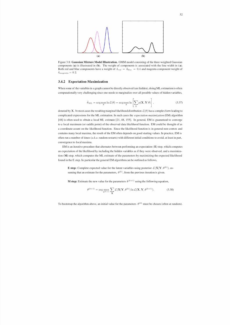
8/13/2019 Continuous-State Graphical Models for Object Localization, Pose Estimation and Tracking
http://slidepdf.com/reader/full/continuous-state-graphical-models-for-object-localization-pose-estimation 67/220
52
(a) (b)
Figure 3.8: Gaussian Mixture Model Illustration. GMM model consisting of the three weighted Gaussian
components (a) is illustrated in (b). The weight of components is associated with the line width in (a).
Both red and blue components have a weight of δ red = δ blue = 0.4 and magenta component weight of
δ magenta = 0.2.
3.4.2 Expectation-Maximization
When some of the variables in a graph cannot be directly observed (are hidden), doing ML estimation is often
computationally very challenging since one needs to marginalize over all possible values of hidden variables,
θML = arg maxθ
ln L(θ) = arg maxθ
ln
X
p(X,Y|θ)
, (3.37)
denoted byX. In most cases the resulting marginal likelihood distributionL(θ) has a complex form leading to
complicated expressions for the ML estimation. In such cases the expectation-maximization (EM) algorithm
[48] is often used to obtain a local ML estimate [21, 48, 155]. In general, EM is guaranteed to converge
to a local maximum (or saddle point) of the observed data likelihood function. EM could be thought of as
a coordinate assent on the likelihood function. Since the likelihood function is in general non-convex and
contains many local maxima, the result of the EM often depends on good starting values. In practice, EM is
often run a number of times (a.k.a. random restarts) with different initial conditions to avoid, at least in part,
convergence to local maxima.
EM is an iterative procedure that alternates between performing an expectation (E) step, which computes
an expectation of the likelihood by including the hidden variables as if they were observed, and a maximiza-
tion (M) step, which computes the ML estimate of the parameters by maximizing the expected likelihood
found in the E step. In particular the general EM algorithm can be outlined as follows,
E step: Complete expected value for the latent variables using posterior L(X|Y, θ(k)), as-
suming that an estimate for the parameters, θ(k), from the previous iteration is given.
M step: Estimate the new value for the parameters θ(k+1) using the following equation,
θ(k+1) = arg maxθ(k+1)
X
L(X|Y, θ(k)) ln L(X,Y, θ(k+1)). (3.38)
To bootstrap the algorithm above, an initial value for the parameters θ(0) must be chosen (often at random).

8/13/2019 Continuous-State Graphical Models for Object Localization, Pose Estimation and Tracking
http://slidepdf.com/reader/full/continuous-state-graphical-models-for-object-localization-pose-estimation 68/220
53
θ
X
θ
xi
N
µ Σ
xi
N
θ
X
Z
θ
xi
z i
N
δ 1 δ M
µ1
µM
Σ1
ΣM
xi
z i
N
.
..
.
..
· · ·
(a) (b) (c) (a) (b) (c)
Gaussian (Normal) Density Model Gaussian Mixture Model
Figure 3.9: Graphical Models for Gaussian and Gaussian Mixture Model. In (a) graphical models for
the Gaussian and Gaussian Mixture Model (GMM) are shown on the (left) and (right) respectively. In (b)
a graphical representation of a Gaussian and GMM for a set of N i.i.d. samples xi is shown. In the case
of GMM (right) corresponding latent cluster labels zi are also shown. In (b) we also introduce a new plate
notation [32], denoted by the box with a label N . Using plates, N instances of the content in the box are
represented compactly by the notation shown. Lastly in (c) all the parameters of the two models are explicitly
shown, instead of a parameter vector θ. Notice that models depicted in (a) are useful for inference, and
models in (b) and (c) for parameter estimation.
The algorithm above iterates until convergence, i.e. θ(k+1) ≈ θ(k).
Expectation-Maximization for Gaussian Mixture Model
A Gaussian or other unimodal distributions in theexponential family are often too restrictive to model realistic
multi-modal data; a Gaussian Mixture is a convienient distribution for modeling such cases. A Gaussian
Mixture is the model with M mixture components, as is shown in Figure 3.8, each of which in themselves
are Gaussian. It is worth noting that Gaussian Mixture is not part of the exponential family of distributions
introduced in Section 3.1.1. Nevertheless Gaussian mixture has a number of convienient properties 2 that are
inherited from the Gaussian components. The model can be written as follows,
p(X|θ) =Z
p(X|Z, θ) p(Z), (3.39)
whereZ is a multinomial hidden indicator variable that tells which mixture component generated the observa-
tion X. For a given value of the indicator p(Z = m), the observation has a normal distribution N (µm, Σm),
m ∈ M .
Alternatively this model can be written in the following form:
p(X
|θ) =
M
m=1
δ m N
(X
|µm, Σm), (3.40)
where θ = µ1, Σ1, δ 1,...,µM , ΣM , δ M andM m=1 δ m =
M m=1 p(Z = m) = 1. Intuitively, the model
tells us that the data is generated by first sampling zi ∼ p(Z) and then given zi sampling from the respective
Normal mixture component. Since clearly we cannot observe zi and are only able to observe the final xi ∼2 Similar to the Gaussian, a product of Gaussian Mixtures is in itself a Gaussian Mixture. Also, the conditional distribution of two or
more variables that jointly have a Gaussian Mixture form, is also a Gaussian Mixture.

8/13/2019 Continuous-State Graphical Models for Object Localization, Pose Estimation and Tracking
http://slidepdf.com/reader/full/continuous-state-graphical-models-for-object-localization-pose-estimation 69/220
54
Input: number of mixture components, M , assumed in the model
N i.i.d. observations x1, x2,...xN drawn from p(X)
initial estimates for parameters θ(0) = θ(0)1 ,...,θ
(0)M , where θ
(0)m = µ
(0)m , Σ
(0)m , δ
(0)m ,
m ∈ [1,...,M ] (typically obtained using K -means)
Output: estimates for parameters θ = θ1,...,θM , where θm = µm, Σm, δ m
E step: Complete expected value for the latent variables z1, z2,...,zN using posterior
p(Z|X, θ(k)), assuming that an estimate for the parameters, θ(k), from the previous iteration
is given:
p(zn = m|xn, θm) = p(xn|zn = m, θm) p(zn = m)M i=0 p(xn|zn = i, θi) p(zn = i)
, (3.41)
where n ∈ [1,...,N ].
M step: Estimate the new value for the parameters θ(k+1) using the following equations,
θ(k+1) = arg maxθ(k+1)
Z
p(Z|X, θ(k)) ln p(X|Z, θ(k+1)), (3.42)
which translates to the following set of equations for individual parameters:
δ (k+1)m =
1
N
N n=1
p(zn = m) (3.43)
µ(k+1)m =
N n=1 p(zn = m)xnN n=1 p(zn = m)
(3.44)
Σ(k+1)m =
N n=1 p(zn = m)(xn − µ(k+1)
m )(xn − µ(k+1)m )T N
n=1 p(zn = m)(3.45)
Loop: Repeat above for a fixed number of iterations, K , or until θ(k+1) ≈ θ(k) (up to some
chosen precision ǫ), then let θ = θ(k+1).
Algorithm 1: Expectation-Maximization for Gaussian Mixture Model. Iterative algorithm for obtaining
estimates for the parameters of the Gaussian Mixture Model (GMM).
p(X |Z = zi, θ), doing direct Maximum Likelihood estimation of the parameters becomes very complicated.
Using EM, however, parameters can easily be derived using the iterative approach described in Algorithm 1.
3.4.3 Parameter Estimation with Hyperpriors
So far we have made an explicit distinction between parameters of the model and the variables associated with
the model (see Figure 3.10 (a)). However, there is nothing special about the parameters and we can treat them
as latent random variables themselves (see Figure 3.10 (b)) [19, 137]. In a Bayesian sense, the parameters
can be reinterpreted as variables and have priors imposed on them much like the variables themselves do (see
Figure 3.10 (c)). These priors are often called hyperpriors. This was already alluded to in Section 3.2.3. For
example, in the case of Gaussian Mixtures it is often convienient to impose a symmetric Dirichlet prior with
concentration parameter α/M on the mixture weights,

8/13/2019 Continuous-State Graphical Models for Object Localization, Pose Estimation and Tracking
http://slidepdf.com/reader/full/continuous-state-graphical-models-for-object-localization-pose-estimation 70/220
55
θ
xi
z i
N
xi
z i
δ 1 δ M
µ1
µM
Σ1
ΣM N
......
· · ·
α
X
Z
δ 1 δ M
µ1
µM
Σ1
ΣM N
......
· · ·
(a) (b) (c)
Figure 3.10: Gaussian Mixture Model with Hyperpriors. Graphical model representation for N i.i.d. sam-
ples drawn from the Gaussian Mixture Model (GMM) is shown in (a). In (b) the same model is shown where
the parameters of the model are treated as variables themselves, on which a hyperprior with hyperparameters
α is imposed in (c).
p(δ 1, δ 2,...,δ M |α) ∼ Dir(α/M, ...,α/M ) = Γ(α)Γ(α/M )M
M m=1
δ α/2−1m . (3.46)
By letting M → ∞ we get an infinite model that allows inference over the number of mixtures in addition
to the parameters of the mixtures themselves. In fact, in the Bayesian sense the parameters are just nuisance
variables that should be integrated out. For details on the use of hyperpriors in graphical models we refer
reader to [107].
3.5 Inference
Given a graphical model encoded by the graph
G =
V ,
Eand a set of known (or estimated) parameters θ,
typically one is interested in inferring the posterior distribution p(X|Y, θ) from the joint p(X,Y|θ) distri-
bution encoded by the model, where X is the set of hidden or latent variables and Y is the set of observed
variables. Sometimes, we are only interested in a subset of variables XU ⊂ X, in which case only the
marginals,
p(XU ) =
X\XU
p(X|Y, θ) dX \XU or p(XU ) =X\XU
p(X|Y, θ) (3.47)
(depending on whether the variables are continues or discrete) are needed.
In fact in most situations computing the full posterior p(X|Y, θ) is prohibitivelyexpensive, and marginalsare computed and used as a summary of the posterior instead. Typically it suffices to estimate the marginals
for all or some subset of variables. For example, given a joint distribution p(X) = p(X1,X2,X3,X4,X5)
encoded in directed graphical model illustrated in Figure 3.2, compute p(X1). Alternatively, we may want
to compute all marginals, p(Xi), i ∈ [1,..., 5]. Using the marginals we can also easily compute conditional
distributions of the form p(XU |X \XU ,Y, θ), where XU is as before subset of variable that are of interest,
and X \XU are all hidden variables excluding those in XU .

8/13/2019 Continuous-State Graphical Models for Object Localization, Pose Estimation and Tracking
http://slidepdf.com/reader/full/continuous-state-graphical-models-for-object-localization-pose-estimation 71/220
56
In this section we will discuss some approaches for doing inference in various graphical models intro-
duced thus far. In particular, we will discuss the Elimination algorithm and the Belief Propagation (specifi-
cally the sum-product) algorithm. For additional information on other popular approaches to inference that
are not covered in the thesis (e.g. junction-tree algorithm [26, 105, 246], mean field [68, 254], variational
inference [109, 238]) we refer reader to the literature.
3.5.1 Variable Elimination
Let us consider the directed graph in Figure 3.2, that has the joint distribution
p(X) = p(X1,X2,X3,X4,X5) = p(X5|X3) p(X4|X2,X3) p(X3|X1) p(X2|X1) p(X1). (3.48)
Let us further assume that all variables in the graph Xi, i ∈ [1, 5] are discrete with L possible states, and
we want to compute the marginal p(X1,X2,X3,X4) =
X5
p(X1,X2,X3,X4,X5). Doing this explicitly
will results in the computation time that has complexity exponential in the number of variables in the jointdistribution, O(L5). However, by taking advantage of conditional independence properties encoded by the
graph structure and distributing the sum by moving it all the way in,
p(X1,X2,X3,X4) = p(X4|X2,X3) p(X3|X1) p(X2|X1) p(X1)X5
p(X5|X3), (3.49)
we get an algorithm that has complexity that is quadratic in the number of discrete states, O(L2). The Variable
Elimination (VE) algorithm [47, 258] does precisely this by rearranging terms of the product making up the
joint distribution and moving the summations as far as possible inward. It is also convienient to introduce
variables mi(XS i ), where S i ⊂ V corresponds to variables that appear in the sum but are not being summed
over. These intermediate variables are called messages. For example, if we want to compute marginal p(X1)for the same graph in Figure 3.2:
p(X1) =X2
X3
X4
X5
p(X1,X2,X3,X4,X5)
=X2
X3
X4
X5
p(X5|X3) p(X4|X2,X3) p(X3|X1) p(X2|X1) p(X1)
=X2
X3
X4
p(X4|X2,X3) p(X3|X1) p(X2|X1) p(X1)X5
p(X5|X3)
m5(X3 )
=X2
X3
X4
p(X4|X2,X3) p(X3|X1) p(X2|X1) p(X1)m5(X3)
=X2
X3
p(X3|X1) p(X2|X1) p(X1)m5(X3)X4
p(X4|X2,X3)
m4 (X2,X3)
=X2
X3
p(X3|X1) p(X2|X1) p(X1)m5(X3)m4(X2,X3)

8/13/2019 Continuous-State Graphical Models for Object Localization, Pose Estimation and Tracking
http://slidepdf.com/reader/full/continuous-state-graphical-models-for-object-localization-pose-estimation 72/220
57
=X3
p(X3|X1) p(X1)m5(X3)X2
m4(X2,X3) p(X2|X1)
m2 (X1,X3)
=X3
p(X3|X1) p(X1)m5(X3)m2(X1,X3)
= p(X1)X3
m5(X3)m2(X1,X3) p(X3|X1) m3 (X1)
= p(X1)m3(X1).
Notice that the complexity of the algorithm is governed by the maximum message size. The algorithm
described above is called Variable Elimination, in essence, because it eliminates one variable at the time from
the graph, until the graph corresponding to the marginal is left. Notice that while the order of the elimination
is not unique3 there is an overall flow that can be established in that we first must eliminate children nodes
(nodes that have no outgoing edges), then their parents and so on.
Notice that a similar elimination procedure can be done if Xi, i ∈ [1,..., 5] are continuous and notdiscrete, in which case the sums in the above formulation will be replaced by the integrals over the continuous
random variables. For example,
p(X1) =
X2
X3
X4
X5
p(X1,X2,X3,X4,X5) dX2 dX3 dX4 dX5
=
X2
X3
X4
X5
p(X5|X3) p(X4|X2,X3) p(X3|X1) p(X2|X1) p(X1) dX2 dX3 dX4 dX5.
Computing marginals in the graph where variables are both discrete and continuous would involve integrating
and summing over the respective variables. So far we have only considered directed graphical models, but
the Elimination algorithm works for undirected graphs as well in a similar manner. Consider computing the
the marginal p(X2) for the graph illustrated in Figure 3.6. Similar to above,
p(X2) =X1
X3
X4
X5
p(X1,X2,X3,X4,X5)
=X1
X3
X4
X5
1
Z ψ123(X1,X2,X3)ψ234(X2,X3,X4)ψ35(X3,X5)
= X1X3
X4
1
Z
ψ123(X1,X2,X3)ψ234(X2,X3,X4)X5
ψ35(X3,X5)
m5(X3 )
=X1
X3
X4
1
Z ψ123(X1,X2,X3)ψ234(X2,X3,X4)m5(X3)
3 In the example discussed,X4
can be done beforeX5
, or theX2
beforeX3
, without effecting the complexity.

8/13/2019 Continuous-State Graphical Models for Object Localization, Pose Estimation and Tracking
http://slidepdf.com/reader/full/continuous-state-graphical-models-for-object-localization-pose-estimation 73/220
58
=X1
X3
1
Z ψ123(X1,X2,X3)m5(X3)
X4
ψ234(X2,X3,X4)
m4(X2,X3 )
=
X1 X3
1
Z ψ123(X1,X2,X3)m5(X3)m4(X2,X3)
=X3
1Z
m5(X3)m4(X2,X3)X1
ψ123(X1,X2,X3)
m1(X2,X3)
=X3
1
Z m5(X3)m4(X2,X3)m1(X2,X3)
= 1
Z
X3
m5(X3)m4(X2,X3)m1(X2,X3)
m3 (X2)
= 1
Z m3(X2).
The key observation with undirected variant is that the normalizing constant, Z , can be factored out in all
but the last step. This significantly simplifies computation of Z , that is typically unknown. By delaying the
computation of Z to the very end, we can compute it by summing over a single variable Z = X2
m3(X2);
computing it beforehand would result in summation over all variables.
One shortcoming of the Elimination algorithm is that while it is efficient for computing single marginals,
it is inefficient for computing marginals over all the variables. The reason for this is that it requires re-
computation of the sums (or messages) for every marginal. However, it is easy to see that these messages will
always be the same (though for an individual marginal not all messages mey be required to be computed).
Reusing these messages is essential in tractable computation of an arbitrary set of marginals. This is the
premise behind the Belief Propagation algorithm outlined in the next section.
3.5.2 Belief Propagation
Belief Propagation (BP) is a popular inference algorithm for computing marginals of functions on undirected
graphical models. BP is an instance of the more general sum-product algorithm that operates on factor
graphs [119]. It can be proved that BP is guaranteed to converge to the exact marginals on tree-structured
graphs [108]. In graphs that contain cycles BP, often in this case referred to as Loopy Belief Propagation
(LBP), can lead to a tractable approximation to the marginals (exact inference is NP-hard [43]). LBP is
not guaranteed to converge, however, and in case of convergence will only converge to a fixed point (not
necessarily corresponding to a true marginal). It can be shown that the fixed point of LBP is equivalent to thestationary point of the Bethe approximation of the free energy [255], hence LBP will always lead to a lower
energy state. In practice, LBP is widely used and has excellent empirical performance in many applications
[221]. Most BP algorithms in the literature have concentrated on the models where variables corresponding
to the nodes in the graph are discrete, however recently, attempts have been made in proposing approximate
inference algorithms that can deal with continuous-state graphs of arbitrary topology [99, 220]. Table 3.1
outlines the various flavors of Belief Propagation algorithms, the details of which will be discussed in the
following sections.

8/13/2019 Continuous-State Graphical Models for Object Localization, Pose Estimation and Tracking
http://slidepdf.com/reader/full/continuous-state-graphical-models-for-object-localization-pose-estimation 74/220
59
Discrete-state Continues-stateGau ssian ( GBP) Non -Gau ssian ( NBP)
Tree Loopy Graph (LBP) Tree Loopy Graph Tree Loopy Graph
Joint, p(X) = 1Z
(i,j)∈A ψij(Xj ,Xi)
i∈[1,...,N ]φi(Xi)
Message,m(Xi) = 1Z
Xi
ψij(Xi,Xj)φi(Xi)k∈A(i)\j mki(Xi) = 1
Z
Xi
ψij(Xi,Xj)φi(Xi)k∈A(i)\j mki(Xi) dXi
Marginal, b(Xi) = 1Z φi(Xi)
k∈A(i) mki(Xi)
Estimated Marginals b(Xi) exact approximate exact exact approximate approximate
Representationof m(Xi) e xact exact exact exact approximate approximate
Complexity O(NL
2
) / O(NL) O(NL
C
) O(N ) O(NDM
2
)N – Number of nodes in a graphL – Number of discrete states
C – Size of the largest clique, defined as the largest set of fully connectednodes, in the graph.D – Largest degree, defined as the number of edgesincident on the node, of the node in a graph.M – Number of components requiredto represent the message.
Table 3.1: Inference using Belief Propagation. Summary of the known BP algorithmvariants with complex-
ity and known theoretical limitations. We will use the continuous-state Non-parametric Belief Propagation
(NBP) approach of [99] on loopy-graphs designated in bold. For further description, including description of
equations, please see text.
Discrete Belief Propagation
Belief propagation can, in general, be introduced in the context of the pair-wise MRF formulation [253]of Section 3.3.2. Consider a set of latent (a.k.a. hidden) variable nodes X = X1,X2,...,XN and a
corresponding set of observed nodes Y = Y1,Y2,...,YN . Please note that 1-to-1 correspondence of the
latent and observation nodes is simply for notational convenience and is not required by the framework or
inference algorithm. The conditional independence of the latent variables is expressed by a neighborhood set
A. A pair of node indices (i, j) ∈ A if the node Xj is not conditionally independent of Xi given all other
nodes in the graph. For notational simplicity we will define a function A(i) that will return all neighbors of i.
More formally j ∈ A(i) ⇐⇒ (i, j) ∈ A. When Xi are discrete random variables, we can assume, without
loss of generality, that they can take on some value xi ∈ [1, 2,...,L]. The observation and hidden nodes
are related by the real-valued observation (or likelihood) function φi(Xi,Yi) ≡ φi(Yi|Xi) ≡ φi(Xi);
connected hidden nodes by a potential (or correlation) function ψij(Xj ,Xi). The joint probability overX = X1,X2,...,XN can then be written as:
p(X) = 1
Z
(i,j)∈A
ψij(Xj ,Xi)
i∈[1,...,N ]
φi(Xi), (3.50)
where Z is a normalizing constant that ensures that p(X) integrates to 1.
A brute force inference algorithm that simply enumerates all possible states for X and evaluates p(X),
would lead to O(LN ) run-time (as was already discussed in Section 3.5.1), which is infeasible even for small
values of L and N . BP that exploits the conditional independence structure of the graphical model would
lead to a solution, that allows computation of arbitrary sub-set of marginals, in O(N LC ), where C ≪ N .
The BP algorithm operates in two stages: (1) it introduces auxiliary random variables mij(Xj) that can be
intuitively understood as messages from hidden node i to node j about what state node j should be in, and
(2) computes the approximation to the marginal distribution of Xi (often refereed to as the belief). Messages
are computed iteratively using the equation below
mij(Xj) ∝Xi
ψij(Xi,Xj)φi(Xi)
k∈A(i)\jmki(Xi), (3.51)

8/13/2019 Continuous-State Graphical Models for Object Localization, Pose Estimation and Tracking
http://slidepdf.com/reader/full/continuous-state-graphical-models-for-object-localization-pose-estimation 75/220
60
Message Passing Belief Estimation
Xj Xi
Yi
←↓
←
↑
Xi
Yi
↓→ ←
↑
mij(Xj) ∝Xi
ψij(Xi,Xj)φi(Xi)
k∈A(i)\j mki(Xi) bi(Xi) ∝ φi(Xi)
k∈A(i)mki(Xi)
Figure 3.11: Belief Propagation. On the left a new outgoing message, in red, is computed from local
image evidence and incoming messages from neighboring nodes, in blue. On the right approximate marginal
densities are determined from the normalized product of the local observations with messages sent from all
neighboring nodes.
and beliefs, where required, are given by
bi(Xi) ∝ φi(Xi)
k∈A(i)
mki(Xi). (3.52)
It should be noted that in the case of tree structured graphs each message is only needs to be sent/computed
once. The algorithm will first send messages from all leaf nodes to the vertices adjacent to the respective
leafs and then will continue sending messages up to the root and then back down towards the leafs until all
messages have been sent exactly once. In this case of the describe tree-structured graphs, BP sometimes is
also refereed to as the Veterbi algorithm [234] or forward-backward algorithm. Consequently, in the case of
the loopy graphs the algorithm needs to iterate and send a complete set of messages a number of times. In
the case of the loopy graph the order in which messages should be sent is not explicitly defined by the graph,
hence a schedule according to which messages should be sent has to be defined.
The complexityof the proposed discrete BP algorithmis O(N L2) for tree structuredmodels and O(N LC )
for loopy graphs, where N is the number of nodes in the graph, L a fixed number of discrete states each Xi
can assume, and C is the size of the maximal clique in the graph. Hence, it is only tractable with relatively
few states L. Recently, it has been shown [59] that for tree structured models with a particular restrictive
choice of ψij(Xj ,Xi) = N (Xi −Xj|µij, Σij) the inference can be done in O(N L). This allows tractable
inference in models that contain on the order of 1 million states.
Discrete Belief Propagation for Articulated Pose Inference
One application of discrete pair-wise MRFs and BP that is directly related to this thesis, was introduced by
Felzenszwalb et al. in [59] and later extended in [121, 122]. The key idea in these methods is to model an
articulated structure (a person) in 2D using a discrete graphical model and formulate the articulated pose
estimation as inference in this graphical model, computed using BP. In this graphical model each node, i, in
the graph corresponds to the body part and the corresponding discrete random variable, Xi, to the pose of
this body part in the image space. The edges in the graph encode the kinematic and joint constraints, ensuring
that the parts are loosely connected. The pose for each part is encoded using a state vector ∈ R4, allowing
to account for x- and y- positions, scale, and rotation of the part in the image. In [59, 122] the state of each

8/13/2019 Continuous-State Graphical Models for Object Localization, Pose Estimation and Tracking
http://slidepdf.com/reader/full/continuous-state-graphical-models-for-object-localization-pose-estimation 76/220
61
variable in the graph Xi, was discretized to 70 x- and y- positions, 10 scales and 32 rotations, leading to
a total of 70 × 70 × 10 × 32 = 1, 568, 000 possible discrete states for each variable Xi. Even with such
relatively coarse discretization, that can lead to as much as 3-pixel and 5.6-degree quantization error for a
typical 640×480 image, inference using BP in a graph of general topology with unconstrained choice for the
potentials is impractical (see Table 3.1). To ensure that inference is computationally tractable, tree-structure
for the graphical model was assumed [59]. This leads, in general, to quadratic inference complexity in the
number of states. However, with such a large state space even this is impractical. The restrictive choice of
the potential functions [59], ψij(Xj ,Xi) = N (Xi−Xj ; µij, Σij), however, led to tractable linear inference
in O(N L).
In this thesis we consider a more general case of this model, by modeling the body using a richer con-
tinuous state graphical model. Notice, that in the case of the 3D pose (being addressed in this thesis) dis-
cretization of the state Xi ∈ R6, similar to the one introduced in [59], would lead to ≈ 1.721 × 10¹³ states
rendering even linear complexity discrete BP methods intractable. Furthermore, the imposed tree structure
requirement of [59, 122] does not allow models that incorporate natural constraints such as those related to
inter-penetrations or occlusions. Incorporating such constraints would lead to loops in the graphical model
structure. The benefit of these richer constraints will be discussed in detail in Chapters 5 and 6. The required
choice of ψij(Xj ,Xi) is also too restrictive to model realistic statistical relationships between variables. For
example, joint limits are hard to model using these simple Gaussian distributions. In this thesis we introduce
a richer class of models that are able to address these issues.
Continuous Belief Propagation
When Xi’s are continuous random variables as is true for our case, the equation for the message (Eq. 3.51)
must be rewritten as follows,
mij(Xj) ∝ Xi
ψij(Xi,Xj)φi(Xi) k∈A(i)\j
mki(Xi) dXi, (3.53)
by replacing the sum with an integral over Xi. Note that the joint distribution p(X) and belief b(Xi) in the
continuous case can be written identically to discrete version above (see Eq. 3.50 and Eq. 3.52 respectively).
If ψij(Xi,Xj) and φi(Xi) are both Gaussian then the marginal distribution at each node is also Gaussian
(regardless of the graph topology) and the integration can be performed exactly [244]. However, this case is
restrictive and uncommon. In most vision problems both the likelihoods and potentials are multi-modal and
non-Gaussian. For simplicity and without loss of generality let us assume that we can model ψij(Xi,Xj) and
φi(Xi) in such cases using a Gaussian mixture model. It can then be shown that the representation required to
represent the messages and the marginals in this case grows exponentially (and in the case of the loopy-graphs
without bound [117]) and has to be approximated to produce tractable inference algorithms. This gives rise
to what are called Non-parametric Belief Propagation (NBP) algorithms that tend to approximate messages
using fixed-length kernel densities and integrals by Monte-Carlo integration. We will describe the extention
to the variant of NBP first introduced in [99], called Particle Message Passing (PAMPAS), in Section 3.7.
However, to do so, we must first introduce the class of Monte Carlo methods.

8/13/2019 Continuous-State Graphical Models for Object Localization, Pose Estimation and Tracking
http://slidepdf.com/reader/full/continuous-state-graphical-models-for-object-localization-pose-estimation 77/220
62
3.6 Monte Carlo Methods
In many cases inference and learning approaches introduced in Sections 3.5.1 and 3.5.2 are intractable, es-
pecially in the cases of continuous variables, and complex multi-modal distributions. Monte Carlo (MC)
methods [138, 175], introduced as early as 1949 by Metropolis and Ulam [141], provide a numeric ap-
proximation to these tasks by using samples of densities instead of densities themselves. In principle MCapproximations can be shown to lead to exact solutions as the number of samples N → ∞. In practice,
computational resources often require inference using a relatively small number of samples, in which cases
the success of the MC method depends on the efficency of the designed sampling scheme.
The key observation, is that many inference tasks over continuous variables can be expressed as the
expectation of some appropriately chosen function f (X), E[f (X)], such that
E[f (X)] =
X
f (X) p(X) dX (3.54)
where p(X), X
∈ Rd, is the target density we are trying to approximate. If we approximate p(X) using N
independent weighted samples s(n), w(n)|n ∈ [1,...,N ], where theN n=1 w(n) = 1, then we can write
E[f (X)] =
X
f (X) p(X) dX ≈N n=1
w(n)f (s(n)). (3.55)
3.6.1 Importance Sampling
The basic MC approximation assumes that we can sample from the target distribution, s(n) ∼ p(X), in
which case w(n) = 1/N . In most cases, in particular in most vision applications, this is typically intractable.
Importance sampling [214] can be used in such cases to facilitate the inference. In particular, let us assume
we have a proposal distribution q (X) that is easy to sample. The expectation can then be re-written as,
E[f (X)] ≈N n=1
w(n)f (s(n)) =
N n=1
w(n) f (s(n)) p(s(n))
q (s(n)) , (3.56)
where s(n) ∼ q (X). The equation simplifies to
E[f (X)] ≈N n=1
w(n)f (s(n)) (3.57)
if we let
w(n) = 1Z w(n) p(s
(n)
)q(s(n) ) , Z =
N i=1
w(i) p(s
(i)
)q(s(i) ) . (3.58)
Hence, importance sampling estimates the target expectation via a collection of weighted samples from
the proposal density s(n), w(n)|n ∈ [1,...,N ]. The choice of the importance function q (X) will dictate
the effectiveness of the proposed approximation. Designing good proposal functions is critical for tractable
inference. Building good proposal functions, however, is hard; particularly in high-dimensional state spaces.
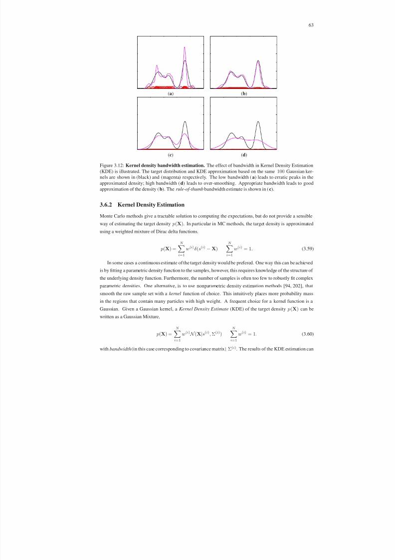
8/13/2019 Continuous-State Graphical Models for Object Localization, Pose Estimation and Tracking
http://slidepdf.com/reader/full/continuous-state-graphical-models-for-object-localization-pose-estimation 78/220
63
(a) (b)
(c) (d)
Figure 3.12: Kernel density bandwidth estimation. The effect of bandwidth in Kernel Density Estimation
(KDE) is illustrated. The target distribution and KDE approximation based on the same 100 Gaussian ker-
nels are shown in (black) and (magenta) respectively. The low bandwidth (a) leads to erratic peaks in the
approximated density; high bandwidth (d) leads to over-smoothing. Appropriate bandwidth leads to good
approximation of the density (b). The rule-of-thumb bandwidth estimate is shown in (c).
3.6.2 Kernel Density Estimation
Monte Carlo methods give a tractable solution to computing the expectations, but do not provide a sensible
way of estimating the target density p(X). In particular in MC methods, the target density is approximated
using a weighted mixture of Dirac delta functions,
p(X) =
N i=1
w(i)δ (s(i) −X)
N i=1
w(i) = 1. (3.59)
In some cases a continuous estimate of the target density would be prefered. One way this can be achieved
is by fitting a parametric density function to the samples, however, this requires knowledge of the structure of
the underlying density function. Furthermore, the number of samples is often too few to robustly fit complex
parametric densities. One alternative, is to use nonparametric density estimation methods [94, 202], that
smooth the raw sample set with a kernel function of choice. This intuitively places more probability mass
in the regions that contain many particles with high weight. A frequent choice for a kernel function is aGaussian. Given a Gaussian kernel, a Kernel Density Estimate (KDE) of the target density p(X) can be
written as a Gaussian Mixture,
p(X) =N i=1
w(i) N (X|s(i), Σ(i))N i=1
w(i) = 1. (3.60)
with bandwidth(in this case corresponding to covariance matrix) Σ(i). The results of the KDE estimation can
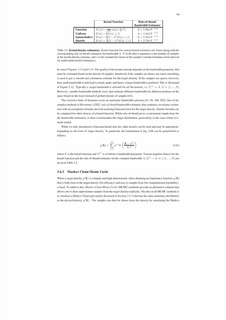
8/13/2019 Continuous-State Graphical Models for Object Localization, Pose Estimation and Tracking
http://slidepdf.com/reader/full/continuous-state-graphical-models-for-object-localization-pose-estimation 79/220
64
Kernel Function Rule-of-thumb
Bandwidth Estimator
Gaussian K(u) = 1√ 2π
exp−1
2 u2
Λ = 1.06σN −1/5
Uniform K(u) = 12 I (|u| ≤ 1) Λ = 1.84σN −1/5
Epanechnikov K(u) = 34
(1 − u2)I (|u| ≤ 1) Λ = 2.35σN −1/5
Quartic
K(u) = 15
16 (1
−u2)I (
|u
| ≤1) Λ = 2.78σN −1/5
Table 3.2: Kernel density estimators. Kernel function for various kernel estimators are listed, along with the
corresponding rule-of-thumb estimators for bandwidth Λ. N in the above equations is the number of samples
in the kernel density estimate, and σ is the standard deviation of the samples (similar formulas can be derived
for multivariate kernel estimators).
be seen if Figures 3.13 and 3.14. The quality of the kernel estimate depends on the bandwidth parameter, that
must be estimated based on the density of samples. Intuitively if the samples are dense, not much smoothing
is need to get a smooth and continuous estimate for the target density. If the samples are sparse, however,
then small bandwidth would lead to erratic peaks and hence a larger bandwidth is prefered. This is illustrated
in Figure 3.12. Typically a single bandwidth is selected for all the kernels, i.e. Σ(i) = Λ, ∀i ∈ [1,...,N ].
However, variable bandwidth methods exist, that estimate different bandwidth for different portions of the
space based on the local (instead of global) density of samples [41].
The extensive body of literature exists on automatic bandwidth selection [41, 94, 186, 202]. One of the
simplest methods is Silverman’s [202] rule-of-thumb bandwidth estimator, that combines covariance estima-
tion with an asymptotic formula; derived assuming Gaussian form for the target density. Similar formula can
be computed for other choices of a kernel function. While rule-of-thumb gives a convienient simple form for
the bandwidth estimation, it often oversmoothes the target distribution, particularly in the cases where it is
multi-modal.
While we only introduced a Gaussian kernel thus far, other kernels can be used and may be appropriate
depending on the form of target density. In particular, the formulation in Eq. 3.60 can be generalized as
follows,
p(X) =
N i=1
w(i)KX− s(i)
Σ(i)
(3.61)
where K is the kernel function and Σ(i) is as before a bandwidth parameter. Various popular choices for the
kernel function and the rule-of-thumb estimates for the common bandwidth Λ, Σ(i) = Λ, ∀i ∈ [1,...,N ],are
given in Table 3.2.
3.6.3 Markov Chain Monte CarloWhen a target density p(X) is complex and high-dimensional, often obtaining an importance function q (X)
that is both close to the target density (for efficency) and easy to sample from (for computational tractability)
is hard. To address this, Markov Chain Monte Carlo (MCMC) methods provide an alternative solution that
allows one to draw approximate samples from the target density explicitly. The idea in all MCMC methods is
to construct a Markov Chain (previously discussed in Section 3.2.1) that has the same stationary distribution
as the desired density p(X). The samples can then be drawn from the density by simulating the Markov

8/13/2019 Continuous-State Graphical Models for Object Localization, Pose Estimation and Tracking
http://slidepdf.com/reader/full/continuous-state-graphical-models-for-object-localization-pose-estimation 80/220
65
Target Density Monte Carlo Approximation KDE Approximation
(a) (b) (c)
Figure 3.13: Non-parametric representation of distribution (coarse). Monte Carlo approximation of the
one-dimensional target distribution p(X) (a) is shown using N = 10 weighted samples. Left column shows
the target distribution being approximated, same in all cases. In (b) different importance/proposal distri-
butions q (X) (blue) and sample-based approximation of the target density based on 10 weighted samples
drawn from these importance distribution (red) are shown. The height of the line representing the sample
corresponds to the normalized importance weight. In (c) continuous approximation to the target distribution
(magenta) obtained by Kernel Density Estimation (KDE) is shown. KDE places a Gaussian kernel (red) at
every sample location obtained in (b). The bandwidth for the kernels was selected using a rule-of-thumb
criterion. Rows of the figure illustrate the effects of different importance function. Top row shows the opti-
mal importance function q (X) = p(X), middle row a good importance function q (X) ≈ p(X), and bottom
row a poor importance function. Clearly the quality of approximation is effected by how well the impor-
tance function matches target distribution. Also notice that rule-of-thumb estimate for the bandwidth tends to
oversmooth the KDE approximation.

8/13/2019 Continuous-State Graphical Models for Object Localization, Pose Estimation and Tracking
http://slidepdf.com/reader/full/continuous-state-graphical-models-for-object-localization-pose-estimation 81/220
66
Target Density Monte Carlo Approximation KDE Approximation
(a) (b) (c)
Figure 3.14: Non-parametric representation of distribution (fine). Monte Carlo approximation of the one-
dimensional target distribution p(X) (a) is shown using N = 100 weighted samples. Left column shows
the target distribution being approximated, same in all cases. In (b) different importance/proposal distri-
butions q (X) (blue) and sample-based approximation of the target density based on 100 weighted samples
drawn from these importance distribution (red) are shown. The height of the line representing the sample
corresponds to the normalized importance weight. In (c) continuous approximation to the target distribution
(magenta) obtained by Kernel Density Estimation (KDE) is shown. KDE places a Gaussian kernel (red) at
every sample location obtained in (b). The bandwidth for the kernels was selected using a rule-of-thumb cri-
terion. Rows of the figure illustrate the effects of different importance function. Top row shows the optimal
importance function q (X) = p(X), middle row a good importance function q (X) ≈
p(X), and bottom row a
poor importance function. Notice that the quality of approximation with 100 samples is considerably better,
than with 10 (see Figure 3.13), in all cases. In fact, a poor choice of the importance function (bottom) to
some extent here is remedied by the relatively large number of samples. As N → ∞, the approximation
approaches the true target distribution regardless of the choice of the importance function (so long as it is
defined on the same domain).

8/13/2019 Continuous-State Graphical Models for Object Localization, Pose Estimation and Tracking
http://slidepdf.com/reader/full/continuous-state-graphical-models-for-object-localization-pose-estimation 82/220
67
Input: target density p(X), that cannot be sampled directly
symmetric proposal distribution q (a|b) = q (b|a)Output: sample x ∼ p(X).
1. Start with some initial value x0, such that p(x0) > 0.
2. For each of t = 0,...,T iterations,
(a) Sample next candidate state x from proposal distribution x ∼ q (·|xt) defined above.
(b) Compute acceptance probability
α = min
p(x)
p(xt), 1
. (3.62)
Notice that since we are computing a ratio, the normalizing constant Z cancels, making
this convienient for cases where partition function cannot be computed explicitly.
(c) Accept the candidate proposal with probability α. In other words draw a random sample
from uniform distribution, r ∼ U (0, 1), and let
xt+1 = x r < α
xt otherwise (3.63)
3. Let x = xT .
Algorithm 2: Metropolis Sampler.
Chain for a number of steps. It can be shown that asymptotically the samples obtained in this way are
unbiased samples from the target density. While finding such a chain sounds hard, it is easy to do in practice.
Simulating the chain is also relatively simple, though it may take a significant amount of time to converge
to the desired distribution. We will now describe a few methods for constructing and simulating the Markov
Chains that have these desired properties.
Metropolis-Hastings Sampler
Let us assume we want to sample from the target density p(X) where sampling directly from p(X) is imprac-
tical (usually because partition function, a.k.a. normalizing constant, Z is hard to compute). Let us further
assume that we have a proposal distribution(a.k.a. jumping distribution) q (a|b) that given a current estimate
for the sample, b, defined on the domain of X proposes an alternative, a. This can be non-informative distri-
bution (e.g. random walk), the only constraint is that this distribution must be symmetric, i.e. q (a|b) = q (b|a).
The Metropolis algorithm [141] generates a sample from the target distribution by running Algorithm 2.
It is easy to see that the outlined algorithm generates a Markov Chain with states
x0, x1,...,xT
since
the state at time t, xt only depends on the state at t − 1. After a sufficiently long generation process this
Markov Chain approaches a stationary distribution and samples from the chain are samples from the target
density p(X).
Hastings [80] generalized the Metropolisalgorithm, to work with an arbitrary proposal function, that must
not be symmetric. In that case the acceptance probability α must be modified to be the following:
α = min
p(x)q (xt|x)
p(xt)q (x|xt) , 1
, (3.64)

8/13/2019 Continuous-State Graphical Models for Object Localization, Pose Estimation and Tracking
http://slidepdf.com/reader/full/continuous-state-graphical-models-for-object-localization-pose-estimation 83/220
68
The resulting algorithm is commonly called Metropolis-Hasting algorithm [80]. Once the samples from
the target distribution are generated in this way, we can of course use them in the Monte Carlo framework to
approximate the desired expectation.
Gibbs Sampler
The Gibbs sampler [75] is a special case of the Metropolis-Hastings sampler where the proposed states are
always accepted, α = 1. Let p(X) be once again the target density we want to sample from. Let us further
assume that the state space can be partitioned in some way, X = X1,X2,...,XN . The Gibbs sampler
samples from p(X) by iteratively sampling from the univariate conditionals of the form p(Xi|X \ Xi) by
keeping N −1 variables fixed at any given time. Such conditional distributions are often easy to simulate, as
opposed to the full joint. Thus a Gibbs sampler simulates N random variables sequentially, rather simulating
all variables at once subject to the joint target distribution.
At any given time t a particular variable i is selected for resampling, and the rest are kept fixed. In the
Metropolis-Hastings algorithm context, the Gibbs sampler can be defined by specifying a particular form for
the proposal distribution,
q (x|x(t)) =
xi ∼ p(Xi|Xj = x(t)
j | j ∈ [1,...,N ] \ i)
xj = x(t)j j ∈ [1,...,N ] \ i
(3.65)
that specifies that the next proposed state from x(t) = x(t)1 , x(t)
2 ,...,x(t)N for a current choice of the variable,
say i = 1, will be x = x1, x(t)2 ,...,x(t)
N sampled according to conditional as stated above. The acceptance
probability for this particular choice of the proposal can be written,
α = min p(x)q (xt|x)
p(xt)q (x|xt)
, 1 (3.66)
= min
p(x1, x
(t)2 ,...,x
(t)N ) p(x
(t)1 |x(t)
2 ,...,x(t)N )
p(x(t)1 ,...,x
(t)N ) p(x1|x(t)
2 ,...,x(t)N )
, 1
(3.67)
= min
p(x1, x
(t)2 ,...,x
(t)N ) p(x
(t)1 , x
(t)2 ,...,x
(t)N ) p(x
(t)2 ,...,x
(t)N )
p(x(t)1 ,...,x
(t)N ) p(x1, x
(t)2 ,...,x
(t)N ) p(x
(t)2 ,...,x
(t)N )
, 1
(3.68)
= min(1, 1) = 1, (3.69)
confirming that we should always accept the proposed state. This analysis holds for any choice of variable i.
Hence, the Gibbs sampler can be more compactly described using Algorithm 3.
As the above equations are iterated, the sample x(t) = x(t)1 , x(t)
2 ,...,x(t)N converges to a sample from
the target density p(X). It has been shown that permuting the order in which the variables are resampled,sometimes improves the rate of convergence. This can be easily done by sampling i in the beginning of each
iteration from uniform discrete distribution, i ∼ U (1, N ).
3.6.4 Sequential Importance Sampling
The Sequential Importance Sampling (SIS), frequently also called Particle Filtering (PF), is a Monte Carlo
(MC) based method that gives rise to an extensive body of literature on sequential Baysian filtering developed

8/13/2019 Continuous-State Graphical Models for Object Localization, Pose Estimation and Tracking
http://slidepdf.com/reader/full/continuous-state-graphical-models-for-object-localization-pose-estimation 84/220
69
Input: set of uni-variate conditional distributions of the following form:
p(X1|X2,X3,...,XN )...
p(Xi|X1,...,Xi−1,Xi+1,...,XN −1)...
p(XN |X1,X2,...,XN −1)Output: sample from the joint x ∼ p(X), where X = X1,X1,...,XN
1. Select an initial value for all variables x(0) = x(0)1 , x
(0)2 ,...,x
(0)N
2. For each t ∈ [1,...,T ] iterations
(a) For each i ∈ [1,...,N ], sample from an appropriate conditional:
x(k)i ∼ p(Xi|x(k−1)
1 ,...,x(k−1)i−1 , x(k−1)
i+1 ,...,x(k−1)N )) (3.70)
x(k)j = x(k−1)
j , j ∈ [1,...,N ] \ i, (3.71)
where k = (t − 1)N + t.
3. Let x = x(TN )1 , x
(TN )2 ,...,x
(TN )N .
Algorithm 3: Gibbs Sampler.
over at least 10 years [9, 54]. Sequential Baysian filtering refers to a class of inference methods that estimate
the values of a variable that evolves over time (often based on some underlying stochastic dynamical sys-
tem/process). The method is commonly called filtering when the estimates are done sequentially in time, it
is also referred to as smoothing when the estimate for the state involves future observations (as in undirected
graphical HMMs), and prediction in cases where one is faced with estimating future values for the evolution
of the system based only on the past observations.Sequential Importance Sampling (SIS) gives rise to a number of variant methods for doing sequential
posterior estimation. In this section we will first introduce the generic SIS approach and then a few variants,
including Sampling Importance Resampling (SIR) (a.k.a. Condensation). The key idea in SIS and Particle
Filteringin general, as with any MC approach, is to approximate the posteriorusing a set of weighted samples.
Let us consider inference in the Hidden Markov Model illustrated in Figure 3.4 ( a). Assuming that we have
a model defined for T time instants, the joint distribution can be written as was discussed in Section 3.2.2,
p(X,Y) = p(Y1|X1) p(X1)T t=2
p(Yt|Xt) p(Xt|Xt−1). (3.72)
We can approximate the desired posterior density, p(X1:T |Y1:T ) = p(X1,...,XT |Y1,...,YT ), that of-
ten cannot be computed directly, using the importance sampling approach introduced in Section 3.6.1. This is
done by introducing an importance density that is easy to sample from, q (X1:T |Y1:T ) = q (X1,...,XT |Y1,...,YT ),
and approximating the desired posterior using a weighted sample set of N samples,
p(X0:T |Y1:T ) ≈N i=1
w(i)1:T δ (X0:T − s(i)
1:T ) (3.73)

8/13/2019 Continuous-State Graphical Models for Object Localization, Pose Estimation and Tracking
http://slidepdf.com/reader/full/continuous-state-graphical-models-for-object-localization-pose-estimation 85/220
70
where
s(i)1:T ∼ q (X1:T |Y1:T ) (3.74)
w(i)
1:T ∝ p(s
(i)1:T
|Y1:T )
q (s(i)1:T |Y1:T )
. (3.75)
Unfortunately this form of inference is often both inconvenient and computationally intractable for two
reasons: (1) it requires devising and sampling from a proposal function in a very high dimensional space
that grows with the number of nodes in the graph, and (2) it requires that the entire process has been ob-
served (batch mode inference). SIS remedies both of these problems by estimating the posterior recursively
(a.k.a. on-line posterior estimation).
Let us assume for the moment that we have a sample based representation of the posterior up to, but
not including, time t, s(i)1:t−1, w(i)
1:t−1|i ∈ [1,...,N ]. If we want to approximate the posterior recursively or
sequentially, and choose an appropriate importance density that factors,
q (X1:t|Y1:t) = q (Xt|X1:t−1,Y1:t)q (X1:t−1|Y1:t−1), (3.76)
then samples from s(i)1:t ∼ q (X1:t|Y1:t) can easily be constructed recursively. This is achieved by taking an
already existing sample based representation for the posterior at time t − 1, and augmenting each particle
s(i)1:t−1 with a sample based estimate of the state at time t, s(i)
t ∼ q (Xt|s(i)1:t−1,Y1:t). The recursive equation
for the weights can also be derived by following rules of importance sampling, resulting in the following:
w(i)1:t ∝ w(i)
1:t−1
p(Yt|s(i)t ) p(s(i)
t , s(i)t−1)
q (s(i)t |s(i)
1:t−1,Y1:t). (3.77)
The equation further simplifies if we assume that we are only interested in the marginal distribution
p(Xt|Y1:t) (a.k.a. filtered estimate) and not the full posterior, in which case the equation for the weights is
reduced to,
w(i)t ∝ w
(i)t−1
p(Yt|s(i)t ) p(s(i)
t , s(i)t−1)
q (s(i)t |s(i)
t−1,Yt). (3.78)
resulting for the sample based representation for the marginal posterior density,
p(Xt|Y1:t) ≈N i=1
w(i)t δ (Xt − s
(i)t ). (3.79)
The outlined approach is the basis of the General Particle Filter, Algorithm 4.
Degeneracy, Impoverishment and Resampling
A common problem with SIS filter is what is frequently known as degeneracy. In particular, often after a few
iterations,all but one sample will have a negligibleweight, contributing virtually nothingto the approximation
of the marginal posterior. In [118] a suitable simple measure of degeneracy was introduced, to measure
effective sample size, N eff , at any given time t,

8/13/2019 Continuous-State Graphical Models for Object Localization, Pose Estimation and Tracking
http://slidepdf.com/reader/full/continuous-state-graphical-models-for-object-localization-pose-estimation 86/220
71
N eff = 1N i=1(w
(i)t )2
(3.80)
Clearly degeneracy effects are undesirable, since they lead to poor approximations of the posterior (at
high computational cost4). The two possible solutions are to either choose a good proposal function, or
to resample the particle set. Even with good proposal functions, often resampling is necessary (but not as
frequently).
The basic idea of resampling is, whenever significant degeneracy is observed (N eff < N th, where N th
is an empirically chosen threshold), to eliminate particles with the low weight, replacing them with particles
that have a more significant support. The resampling is implemented by drawing with replacement a new
set of unweighted samples (representing the same density) s(i)t , w
(i)t |i ∈ [1,...,N ], w
(i)t = 1
N for all
i ∈ [1,...,N ], where the probability of drawing a sample is proportional to the weight of the sample in the
original set s(i)t , w(i)
t |i ∈ [1,...,N ]. In other words, p(s(i)t = s(i)
t ) = w(i)t .
While resampling helps to reduce degeneracy in particle filters, it may introduce other problems. The
most significant of such problems is what often referred to as sample impoverishment , which arises when one
or few particles have a high weight relative to the rest. In such a case the new resampled approximation will
have many repeated samples. This lack of diversity in samples tends to translate into poor approximation of
the posterior. This problem is particularly acute where the process noise is small, often leading to collapse of
all particles to a single sample point.
Sampling Importance Resampling Filter or Condensation
Thus far we have introduced a conceptual Particle Filtering framework that is common to many recursive
Bayesian approaches. To build a realistic algorithm a choice of importance function must be specified. In
this section we will introduce one variant of the Particle Filter called Sampling Importance Resampling (SIR)
[76] or in the computer vision community better known as Condensation introduced by Blake and Isard in[25].
This particular Particle Filter variant is derived by making two assumptions: (1) that we going to use the
temporal prior as a proposal function (i.e. q (Xt|Xt−1,Y1:t) = p(Xt|Xt−1)), and (2) resampling is applied
at every iteration (i.e. N th = ∞). Notice that this choice of importance density assumes a relatively simple
temporal prior from which samples can be generated. In practice, often linear models with Gaussian noise
are chosen for p(Xt|Xt−1) = N (Xt|β Xt−1, Σ). Also notice that since resampling is done at every time
step, the computation of weights reduces to a particularly simple (non-recursive) form,
w(i)t ∝ p(Yt|s(i)
t ), (3.86)
that only depends on the likelihood . This particular variant of a particle filter has been applied extensively to
object tracking in computer vision domain; for discussion and more detailed derivation see Section 2.8.
4 Samples, while contributing little to the overall quality of approximation, still need to be updated in the filtering framework.

8/13/2019 Continuous-State Graphical Models for Object Localization, Pose Estimation and Tracking
http://slidepdf.com/reader/full/continuous-state-graphical-models-for-object-localization-pose-estimation 87/220
72
Input: sample based approximation to the marginal posterior at time t − 1
p(Xt−1|Y1:t−1) ≈ s(i)t−1, w(i)
t−1|i ∈ [1,...,N ]Output: sample based approximation to the marginal posterior at time t
p(Xt|Y1:t) ≈ s(i)t , w
(i)t |i ∈ [1,...,N ]
1. For each sample i ∈ [1,...,N ]
(a) Draw s(i)t ∼ q (Xt|s(i)
t−1,Yt) from proposal function q (·).
(b) Compute the sample weight
w(i)t ∝ w(i)
t−1
p(Yt|s(i)t ) p(s
(i)t , s
(i)t−1)
q (s(i)t |s(i)
t−1Yt). (3.81)
2. Normalize weights for each sample i ∈ [1,...,N ]
w(i)t =
w(i)t
N i=1 w
(i)t
(3.82)
3. Calculate effective sample size
N eff = 1N i=1(w(i)
t )2(3.83)
4. If N eff < N th, resample the particle set by drawing with replacement from the sample based
approximation of the density p(Xt|Y1:t) ≈ s(i)t , w
(i)t |i ∈ [1,...,N ].
(a) For each sample k ∈ [1,...,N ],
s(k)t ∼ s(i)
t , w(i)t |i ∈ [1,...,N ] (3.84)
w(k)
t =
1
N (3.85)
(b) For each sample k ∈ [1,...,N ], let s(k)t = s
(k)t and w(k)
t = w(k)t
Algorithm 4: Generic Particle Filter.
Number of Particles
All particle filters, use a set of N weighted samples to represent the posterior. As the number of samples
N → ∞ the approximation approaches the true posterior, as with standard importance sampling. However,
in practice, due to computational cost, inference must be done with as few samples/particles as possible.
In general, it is hard to automatically select the number of particles needed for good posterior approxima-tion. The number of particles will depend on the structure and shape of the posterior, proximity of proposal
distribution to the true posterior, the complexity of underlying dynamical process, observation noise, and
dimensionality of the state-space. In [136], a lower bound for the number of particles needed, known as
survival rate, is derived. In particular,
N ≥ N minγ d
, (3.87)
8/13/2019 Continuous-State Graphical Models for Object Localization, Pose Estimation and Tracking
http://slidepdf.com/reader/full/continuous-state-graphical-models-for-object-localization-pose-estimation 88/220
73
where N is the lower bound on the number of samples needed, subject to the dimensionality of the state space
d, a survival rate γ ≪ 1 that is a constant related to how well the posterior is approximated by the filter (and
is a function of posterior and proposal distribution shape and complexity); N min is a parameter designating
the minimum number of particles to survive the resampling. The survival rate γ will typically be lower for
noisy posterior distributions that are not modeled well, requiring more samples to represent them adequately.
Consequently, for proposal distributions that are poor approximations to the posterior, γ will be low as well,
leading to similar artifacts. Lastly, the number of samples required to model a high dimensional posterior,
according to this metric, will grow exponentially with the dimensionality of the state-space d. This is known
in computer vision as the curse of dimensionality.
Regularized Particle Filter
The general Particle Filter framework as well as the particular instance of SIR (or Condensation) in the
previous section attempts to resolve the issue of degeneracy with resampling and/or good proposal densi-
ties. However, as mentioned before, resampling often leads to sample impoverishment. At least in part this
problem can be attributed to the fact that when the approximation to the density (encoded using a weightedsample set) is resampled, we are sampling from a discrete representation of the posterior instead of the full
continuous approximation.
A Regularized Particle Filter (RPF) [154] was introduced to remedy this phenomenon. The RPF is identi-
cal to SIR filter introduced in the previous section, in all but one respect. During resampling, RPF resamples
from the continuous approximation of the marginal posterior obtained using Kernel-based approximation
introduced in Section 3.6.2. RPF bears striking similarity to the Particle Message Passing (PAMPAS) [99]
approach, that will be discussed in the next section and used throughout this thesis. In fact, Particle Message
Passing (PAMPAS) is a generalization of the RPF filter that allows inference in graphs of arbitrary topology.
For topology of Hidden Markov Models (HMMs) it can be shown that PAMPAS reduces to RPF.
3.7 Particle Message Passing
Particle filters introduced in the previous section are effective for inference in many different models and
applications, however, they are customized for temporal filtering or estimation problems in Hidden Markov
Models. Belief Propagation introduced in Section 3.5.2 provides the means of effective inference in graphs
of arbitrary topology, however, is typically restricted to discrete variables or continues Gaussian variables
for tractable inference. In this section we will introduce Particle Message Passing (PAMPAS) [99], a variant
of Non-parametric Belief Propagation [220], that is able to perform approximate inference in the graphs of
arbitrary topology and makes no explicit assumptions about parametric form for the variables or potential
functions. In Particle Message Passing we generalize Particle Filters to work for graphs of arbitrary topology.
PAMPAS will underline the inference tasks in this thesis.
As in standard Belief Propagation, introduced in Section 3.5.2, for convenience we will restrict ourselves
to inference in pair-wise MRFs. However, similar results can be derived for a general MRF and Baysian
Networks. A simple extension would lead to variant that would work for factor graphs. Given a pair-wise
Markov Random Field specified by the graph G = V , E, where we have a set of hidden, V X, and observed,
V Y , nodes corresponding to variables X = X1,X2,...,XN and Y = Y1,Y2,...,YM respectively, we

8/13/2019 Continuous-State Graphical Models for Object Localization, Pose Estimation and Tracking
http://slidepdf.com/reader/full/continuous-state-graphical-models-for-object-localization-pose-estimation 89/220
74
can write the joint distribution as follows,
p(X) = 1
Z
(i,j)∈E ,i∈V X,j∈V X
ψij(Xi,Xj)i∈V X
φi(Xi,Y). (3.88)
If we assume thatXi’s are continuous random variables, we can write down the recursive message passing
and belief estimation equations underlying BP (see Section 3.5.2):
Continuous message passing: mij(Xj) ∝ Xi
ψij(Xi,Xj)φi(Xi,Y)
k∈A(i)\jmki(Xi) dXi(3.89)
Belief estimation: bi(Xi) ∝ φi(Xi,Y)
k∈A(i)
mki(Xi). (3.90)
The key observation, underlying both Particle Message Passing and the more general NBP [220], is that
integration required to perform message passing can be approximated using Monte Carlo techniques intro-
duced in Section 3.6. For convenience, we will first formulate PAMPAS for a restricted set of MRFs where
potentials ψij(Xi,Xj) can be expressed using finite Gaussian mixtures and then address the more general
case where some potential functions do not have this convienient form. Notice, that even this more restrictive
case, where potentials can be expressed using finite Gaussian mixtures, produces a considerably richer class
of models then the purely Gaussian MRFs introduced in Section 3.5.2. In its original form, Particle Massage
Passing was introduced by Michael Isard in [99]; here we generalize the original formulation of [99] to make
the approach appropriate for the applications addressed in this thesis.
As in [99], for convenience we first introduce a probability density function that we will call message
foundation (where convenient we will use the following shorthand notation for the likelihood φi(Xi) =
φi(Xi,Y)),
mF ij(Xi) ≡ 1
Z ijφi(Xi)
k∈A(i)\j
mki(Xi), (3.91)
where Z ij is a normalizing constant. Intuitively, the message foundation approximates the distribution over
Xi, that is then used to derive compatible distribution for Xj encoded by the message mij(Xj). We can
use Monte-Carlo integration to approximate the messages by drawing N samples from the message foun-
dation, s(n)ij ∼ mF
ij(Xi)|n ∈ [1,...,N ], and then propagating these samples through a potential function
ψij(Xi,Xj), resulting in the following
mij(Xj) =
N
n=1
w(n)ij ψij(Xi = s(n)
ij ,Xj) (3.92)
mixture approximation to the message, where w(n)ij = 1/N is the weight associated with each sample.
Assuming that ψij(Xi,Xj) can be modeled using a joint distribution represented by the Mixture of M ij
Gaussians (MoG), the resulting mixture distribution,
mij(Xj) = 1
N
N n=1
ψij(Xi = s(n)ij ,Xj) =
1
N
N n=1
ψij(Xj |Xi = s(n)ij ), (3.93)

8/13/2019 Continuous-State Graphical Models for Object Localization, Pose Estimation and Tracking
http://slidepdf.com/reader/full/continuous-state-graphical-models-for-object-localization-pose-estimation 90/220
75
for the message will be a Gaussian mixture as well with M ijN components. Notice that by assuming a MoG
form for ψij(Xi,Xj) we can model a large class of potential functions. For tractable inference, however,
M ij must remain small (on the order of tens of components).
In general, we can sample from any importance function, s(n)ij ∼ q ij(Xi)|n ∈ [1,...,N ] so long as
we apply importance re-weighting resulting in non-uniform weight w(n)ij
∝ mF
ij(snij)/q ij(snij). As with any
particle filtering the choice of importance function will effect the convergence properties of the algorithm.
Furthermore, samples can be stratified into a number of groups.
To compute the marginal distribution over Xi, samples can be drawn from the belief distribution bi(Xi)
directly or using importance sampling. These possibly weighted samples (sum of Dirac functions) serve as
an approximate representation of the true marginal. If continuous representation of the marginal is required,
kernel density estimation can be used to smooth the particle set (see Section 3.6.2).
3.7.1 Sampling from a Product of Gaussian Mixtures
The key to inference using PAMPAS is sampling from the message foundation mF ij(Xi). For the moment,
as in previous section, let us assume that both the likelihoods, φi(Xi,Y), and the potentials, ψij(Xi,Xj),can be expressed as mixtures of Gaussians. In that case sampling from mF
ij(Xi) amounts to sampling from a
product of Gaussian mixtures. We will consider a more general case, where only a subset of potentials have
this form in the next section.
Let us consider a case where we have a product of N mixtures of M n, n ∈ [1,...,N ], components respec-
tively, resulting in the product that can be expressed as a mixture itself withN n=1 M n Gaussian components.
Hence, the brute force approach to sampling would require time exponential in the number of mixtures,
O(N n=1 M n) (O(M N ) if for all mixtures M n = M ). This is only tractable for products of few mixtures
(typically N < 3) having relatively few mixture components. To make the sampling tractable, Sudderth
et al. [220] propose a Gibbs sampler (see Section 3.6.3), that can produce the unbiased exact samples from
the product in O(KN M 2), as the number of iterations K → ∞. In practice with a relatively small value of
K a good sampling can be achieved (we typically use 5 < K < 10). In cases where N < 3 the brute force
sampling is tractable, and we use the exact sampler instead.
The Gibbs sampler works by iteratively sampling labels L = l1, l2,...,lN , where ln ∈ [1,...,M n]
corresponding to the Gaussian components in mixture n. Initially L is initialized by randomly sampling the
labels. We found that initializing the sampler by sampling ln’s according to the probability of the mixture
components in the mixture n, as in [220], led to slower convergence is some cases. Once we have an initial set
of labels L, we pick an integer k ∈ [1,...,N ] at random and sample lk according to the marginal distribution
on the labels. The full algorithm introduced in [220] is restated in Algorithm 5 for completeness.
Significant optimizations to the above algorithm can be made for the case where all mixture components
have the same covariance. Similarly, for the specific case of mixtures that have diagonal covariance structure,
an approximate sampling scheme was introduced in [95] that can sample from the product in O(KM N ).
3.7.2 Sampling from More General Forms of Message Foundation
It is impractical to assume that the likelihood φi(Xi,Y) can be explicitly modeled using a Gaussian mixture,
in fact in most cases φi(Xi,Y) willbe too complex to be able to sample fromit directly. It is also possible that
some sub-set of potentials ψij(Xi,Xj) will not be able to be modeled using a Gaussian mixture effectively.

8/13/2019 Continuous-State Graphical Models for Object Localization, Pose Estimation and Tracking
http://slidepdf.com/reader/full/continuous-state-graphical-models-for-object-localization-pose-estimation 91/220
76
Input: D Gaussian mixtures, where mixture d ∈ [1,...,D] contains M d Gaussian components
with parameters w(m)d , µ(m)
d , Λ(m)d respectively.
Output: x ∼ Dd=1
M dm=1 w
(m)d N (µ
(m)d , Λ
(m)d ).
1. For each d ∈ [1,...,D], choose a starting label ld ∈ [1,...,M d] by sampling p(ld = j) ∝1/M d. For convenience, let L = l1, l2,...,lD.
2. For each d ∈ [1,...,D],
(a) Calculate the covariance matrix
Λ⋆ =
d−1i=1
Λ
(li)i
−1
+D
i=d+1
Λ
(li)i
−1−1
(3.94)
and the mean vector
µ⋆ = Λ⋆
d−1
i=1 Λ
(li)i
−1
µ(li)i +
D
i=d+1 Λ
(li)i
−1
µ(li)i
(3.95)
of the Gaussian resulting from taking a product of Gaussians designated by the set of
fixed labels L/ld.
(b) For each m ∈ [1,...,M d] calculate
Λ(m) =
Λ
(ld)d
−1
+ [Λ⋆]−1
−1
, µ(m) = Λm
Λ
(ld)d
−1
µ(ld)d + [Λ⋆]
−1 µ⋆
(c) Sample a new value for label ld according to
p(ld = m) ∝ w(m)d
N (x; µ(m)d , Λ
(m)d ) N (x; µ⋆, Λ⋆)
N (x; µ(m), Λ(m)) (3.96)
where x is any convenient point (we use x = µ(m) ).
3. Repeat step 2 for K iterations.
4. Compute the mean and covariance for the Gaussian component of the product designated by
L.
Λ =
Di=1
Λ
(li)i
−1−1
, µ = Λ
Di=1
Λ
(li)i
−1
µ(li)i
5. Draw sample x ∼ N (µ, Λ).
Algorithm 5: Gibbs Sampler for a Product of Gaussian Mixtures. Original algorithm is introduced in[220].
Hence, we must handle a case where only a sub-set of the terms in the message foundation, mF ij(Xi), will
have the convenient Gaussian mixture form; for convenience let us call the product of those terms mF Sij (Xi).
The rest of the terms that do not have the convenient form from which we can easily sample can be combined
into mF Eij (Xi), such that mF
ij(Xi) = mF Sij (Xi)mF E
ij (Xi). For example, if the likelihoods φi(Xi,Y) are not

8/13/2019 Continuous-State Graphical Models for Object Localization, Pose Estimation and Tracking
http://slidepdf.com/reader/full/continuous-state-graphical-models-for-object-localization-pose-estimation 92/220
77
Gaussian mixtures and potentials ψij(Xi,Xj) are, then mF Sij (Xi) =
k∈A(i)\j mki(Xi) and mF E
ij (Xi) =
φi(Xi,Y).
Of particular interest is the case where some (but not all) potentials can be represented using mixtures
of Gaussians (MoGs). Let us consider a case where a graph contains potentials of two distinct types5
ψ(MoG)ij (Xi,Xj) and ψ
(¬MoG)ij (Xi,Xj). Assuming that the messages are obtained as before by propa-
gating samples via these potentials, this will lead to two corresponding message types, m(MoG)ij (Xj) and
m(¬MoG)ij (Xj). We can now collect all the terms that have a convienient form for sampling into mF S
ij (Xi) =k∈A(i)\j m
(MoG)ki (Xi), and the rest of the terms into mF E
ij (Xi) = φi(Xi,Y)k∈A(i)\j m
(¬MoG)ki (Xi).
The PAMPAS algorithm of Section 3.7 can then be easily modified to handle this case by setting the
importance function q ij(Xi) = mF Sij (Xi). The new NBP variant will then proceed by sampling s
(n)ij ∼
mF Sij (Xi) from the importance function and then the importance re-weighting will assign the weight of
w(n)ij ∝ mF E
ij (s(n)ij ) to the sample. The resulting message will then be obtained as before, by condition-
ing on Xi, i.e. ψij(Xi = s(n)ij ,Xj) = ψij(Xj |Xi = s
(n)ij ).
3.7.3 Choice of Importance Functions
Sections 3.7.1 and 3.7.2 introduce a particular choice of importance function for approximating messages in
BP using Monte Carlo,
q ij(Xi) = mF Sij (Xi). (3.97)
However, this choice of an importance function is not always effective. In particular, consider inference
in an undirected chain (e.g. Hidden Markov Model with 3 hidden random variables – X1,X2,X3). The
limitation is that for messages m12(X2) and m32(X2) the corresponding importance functions q 12(X1) =
mF S12 (X1) = ∅ and q 32(X3) = mF S
32 (X3) = ∅ are non-informative. While the messages will correctly weigh
the non-informative samples, in high-dimensional spaces this will lead to poor approximation to the messages
(see discussion in Section 3.6.1). One solution is to use a different importance function that facilitates place-
ment of samples in high probability regions. One natural choice is to use belief as an importance function. In
other words, let
q ij(Xi) = mF Sij (Xi)mji(Xi). (3.98)
This choice of importance function will also in some cases facilitate faster mixing between messages, leading
to overall faster convergence of BP [99].
In order to use either of the two importance functions, however, messages must be initialized . In discrete
belief propagation messages are often initialized by uniform distributions, that are then refined by Belief
Propagation message passing. In the continuous case, and more specifically in high-dimensional continuous
case, having uniform messages will lead to non-informative importance functions. This in tern will lead to
poor approximation to the true messages, and often will not lead to convergence of NBP. Hence, for the
non-parametric BP inference to be effective, some or all messages must be initialized to semi-informative
distributions6. In most tracking applications [219] this is done by providing an initial pose, or distribution
5 In both cases we assume that conditional distributions of the form ψij(Xi = x,Xj) can be derived analytically.
6 Notice that this is equivalent to having an informative importance function for some of the variables in the graph.
8/13/2019 Continuous-State Graphical Models for Object Localization, Pose Estimation and Tracking
http://slidepdf.com/reader/full/continuous-state-graphical-models-for-object-localization-pose-estimation 93/220
78
over poses at the first frame. In this thesis we take a very different approach. Instead, we assume that there
exists a static discriminative proposal process that provides reasonable starting values or distributions over
those values for some of the variables. In other words that we have an informative proposal for some of the
messages,
q ij(Xi) = f (Xi). (3.99)
In computer vision applications, having a proposal function of this type is often relatively easy. For example,
for articulated body pose estimation, where variables correspond to body parts, finding plausible positions
for some variables corresponding to the placement of salient limbs or a face is a well researched problem
(efficient and effective solutions to which exist).
3.7.4 Stratified Sampling
Stratified sampling (a.k.a. proportional sampling), involves dividing the samples into a set of homogeneous
groups, and sampling within each group according to some function. While stratified sampling is of signifi-
cant importance in probability and statistics by itself, here we will consider stratified sampling in the context
of Monte Carlo methods and PAMPAS. Consider Monte Carlo importance sampling, first introduced in Sec-
tion 3.6.1. As mentioned before, the efficiency of Monte Carlo approximation depends significantly on the
importance function chosen. Sometimes, however, it is unclear which importance function is best suited for
the inference task, and a number of alternative importance functions may be available. In particular, in Sec-
tion 3.7.3 three importance functions have been introduced that are of interest in Particle Message Passing.
The key observation is that instead of drawing all samples from one importance function that is believed to be
most efficient, we can stratify the sampling procedure to draw samples from multiple importance functions.
As a result, the samples will be more diverse overall, yet focused within each group.
Let us assume we have a family of R importance functions, q (r)
ij (X
i), where r
∈ [1,...,R] from which
we want to draw N samples. If we also assume that each importance function has an associated sampling
fraction γ r , such thatRr=1
γ r = 1, then we can define a stratified sampler as follows:
s(k)ij ∼ q
(1)ij (Xi) for k ∈ [1, . . . ,Nγ 1]
s(k)ij ∼ q (2)
ij (Xi) for k ∈ [N γ 1 + 1, . . . ,Nγ 1 + N γ 2]
· · ·
s(k)ij ∼ q
(r)ij (Xi) for k ∈
N r−1
l=1
γ l + 1,...,N r
l=1
γ l
· · ·s(k)ij ∼ q (R)
ij (Xi) for k ∈
N R−1l=1
γ l + 1,...,N
Since the samples, s(k)ij |k ∈ [1,...,N ], will be drawn from different importance functions, importance cor-
rection must also be done accordingly. In particular, if q (r)ij (Xi), r ∈ [1,...,R], are the importance functions

8/13/2019 Continuous-State Graphical Models for Object Localization, Pose Estimation and Tracking
http://slidepdf.com/reader/full/continuous-state-graphical-models-for-object-localization-pose-estimation 94/220
79
for approximating message, mij(Xj), then the following importance correction must be applied,
w(k)ij =
mF ij(s
(k)ij )
q (1)ij (s
(k)ij )
for k ∈ [1, . . . ,Nγ 1]
w(k)
ij =
mF ij(s(k)
ij )
q (2)ij (s(k)
ij ) for k ∈ [N γ 1 + 1, . . . ,Nγ 1 + N γ 2]
· · ·
w(k)ij =
mF ij(s
(k)ij )
q (r)ij (s
(k)ij )
for k ∈
N r−1l=1
γ l + 1,...,N rl=1
γ l
· · ·
w(k)ij =
mF ij(s
(k)ij )
q (R)ij (s(k)
ij )for k ∈
N R−1l=1
γ l + 1,...,N
.
In the above we assumed that N γ i is an integer for all i, in practice this it is often a fraction and must be
rounded. For the stratified sampling to be effective, one must ensure that the number of groups (strata), S , is
relatively small in relationship to the total number of samples, N . In addition, having widely disproportionalfractions of samples may cause sampling artifacts. We found stratified sampling to be effective in P AMPAS.
The full stratified sampling PAMPAS procedure is outlined in Algorithm 6.
3.7.5 Differences between PAMPAS and NBP
While the PAMPAS [99] algorithm introduced here and the Non-parametric Belief Propagation (NBP) algo-
rithm introduced in [220] are very similar in nature, there are two key differences that are worth mentioning.
First, in [220] no particular form for the potentials is assumed. Hence, instead of propagating samples
from the message foundation, s(n)ij |n ∈ [1,...,N ], via a potential resulting in convenient continuous rep-
resentation for the message, in [220] ψij(Xi,Xj) is sampled. This results in a particle representation for
the message and kernel bandwidth estimation is used to assign equal variance bandwidth to all the samples.
This leads to an additional approximation of ψij(Xi,Xj), where as in our case ψij(Xi,Xj), modeled using
Gaussian mixtures7, can be represented exactly.
Second, there is a difference in where the importance sampling takes place due to the inability to represent
likelihoods, φi(Xi,Y), using convenient Gaussian mixture form. In [220] importance sampling and re-
weighting is incorporated directly into the Gibbs sampler. This results in a generally better sampling strategy,
however, requires an underlying assumption that the kernel width is small relative to the variations in the
likelihood function φi(Xi,Y). As a result, we believe that multiple hypothesis in the message foundation
would tend to cause more severe problems in [220], rendering the algorithm of [220] inferior in cases where
good initialization is unavailable. In PAMPAS, we need not make any assumptions on the kernel widthand can represent the potential exactly, which makes it more convenient for the cases where only weak
initialization is available. However, one would expect our approach to degrade as mF ij(Xi) and mF S
ij (Xi)
become more dissimilar (i.e. more terms in the message will not have the convenient Gaussian mixture form),
and in such cases NBP [220] may lead to superior performance.
7 Other potential functions ψij(Xi,Xj) from which conditional distributions of the form ψij(Xi = x,Xj) can be derived analyt-
ically, can also be represented exactly.

8/13/2019 Continuous-State Graphical Models for Object Localization, Pose Estimation and Tracking
http://slidepdf.com/reader/full/continuous-state-graphical-models-for-object-localization-pose-estimation 95/220
80
Input: Graphical model G = V , E with specified robust potential ψij(Xi,Xj) (consisting
of Gaussian mixtures with M ij components and a single Gaussian outlier process)
and likelihood φi(Xi,Y) functions
Set of possibly uninitialized messages mij(Xj)Number of samples to use for approximating the message, N .
Output: Updated message mij(Xj)
1. Collect all terms in the message foundation mF ij(Xi) = 1
Z ijφi(Xi)
k∈A(i)\j mki(Xi), that
have convienient Gaussian mixture form into mF Sij (Xi) term.
2. Set importance functions and corresponding sampling fractions
(a) q (1)ij (Xi) = mF S
ij (Xi) q (2)ij (Xi) = mF S
ij (Xi)mji(Xi) q (3)ij (Xi) = f (Xi)
(b) For the first iteration of BP typically γ 1 = 0, γ 2 = 0, γ 3 = 1, for the rest typically
γ 1 = 0.5, γ 2 = 0.5, γ 3 = 0.
where f (Xi) is the static proposal distribution.
3. For each of the importance functions k ∈ [1,..., 3]
(a) Compute starting sample index, N s = k−1l=1
Nγ kM ij
(b) Draw N k = (N − 1)γ k/M ij samples from the proposal function:
s(N s+n)ij ∼ q
(k)ij (Xi), n ∈ [1,...,N k] (3.100)
(c) Compute importance correction for n ∈ [1,...,N k]
w(N s+n)ij =
mF ij(s
(N s+n)ij )
q (k)ij (s
(N s+n)ij )
(3.101)
4. Assuming that we have a robust potential function for which conditional can be derived,
e.g. for Gaussian mixture potential
ψij(Xj |Xi) = λ0 N (Xj|µ0, Λ0)+(1−λ0 )
M ijm=1
δ ijm N (Xj |F ijm(Xi), Gijm(Xi)), (3.102)
store normalized weights and mixture components for n ∈ [1,..., (N − 1)/M ij], m ∈[1,...,M ij]:
(a) n′ = (n − 1)M ij + m
(b) µ(n′)ij = F ijm(s
(n)ij )
(c) Λ(n′)ij = Gijm(s(n)
ij )
(d) π(n′)ij = (1 − λ0)w
(n)ij δijm
N −1l=1
w(l)ij
5. Assign outlier components: π(N )ij = λ0, µ
(N )ij = µ0, Λ
(N )ij = Λ0
6. Let mij(Xj) =N n=1
π(n)ij N (Xj |µ(n)
ij , Λ(n)ij ).
Algorithm 6: PAMPAS Stratified Message Update.

8/13/2019 Continuous-State Graphical Models for Object Localization, Pose Estimation and Tracking
http://slidepdf.com/reader/full/continuous-state-graphical-models-for-object-localization-pose-estimation 96/220
81
3.7.6 Message Passing Scheduling
While in theory the massage passing schedule (order) in BP does not matter, in practice it has been shown
that the message passing schedule can effect the convergence properties significantly. It is a well-known em-
pirical observation that asynchronous message passing algorithms, where messages are updated sequentially,
generally converge faster and more often than the synchronous variant, where all messages are updated inparallel. In practice, however, synchronous variants are often used, perhaps due to ease of implementation.
In tree-structured graphs the order in which messages should be sent is explicitly defined by the graph. In
this case when sequential updating is used, the standard naive schedule is one where a message is propagated
as soon as all of its inputs are available or have changed. This results in propagation of messages from the
leaves of the tree upward toward the root and then back down.
In general loopy-graphs an explicit message passing schedule must be defined. The message passing
schedule can be either synchronous or asynchronous. Synchronous message passing amounts to simultane-
ously sending messages along all edges of the graph. It has been shown, however, that often this results in
very slow and inefficient convergence [56]. Alternatively, an asynchronous message passing schedule would
lead to passing messages in a serial order defined by the schedule. One of the standard asynchronous messageschedules can be derived by computing a minimum spanning tree over the graph and updating messages ac-
cording to the tree-structurerules [239]. The spanning tree, however, may not be unique. In this case one must
either choose a tree and a fixed asynchronous schedule for that tree, or for every iteration of BP randomly
pick a minimum spanning tree and a corresponding schedule. In this thesis, we use a fixed asynchronous
message passing schedule with a minimum spanning tree, for simplicity. In general, however, better conver-
gence may be achieved by randomizing the tree parameterization and the message passing schedule. More
recently a new informative message scheduling approach [56] has been proposed that schedules messages in
an informed way, that pushes down a bound on the distance from the fixed point.
3.7.7 Simulated Annealing
The Markov chain based method of simulated annealing was developed initially in [116] and later adopted for
articulated particle filtering in [52] and [70] as a way of handling multiple modes in a stochastic optimization
context. The method employs a series of distributions, with probability densities given by p0(X) to pM (X),
in which each pm(X), m ∈ [0,...,M ], differs only slightly from pm+1(X). In this context samples need to
be drawn from p0(X) and pm(X)’s are designed such that in pM (X) the movement between all regions of
the search space are allowed. The usual method is to set pm(X) ∝ [ p0(X)]βm , for 1 = β 0 > β 1 > ... > β M .
In the case of Particle Message Passing (PAMPAS) one can anneal the likelihood, the potentials or both.
In our experiments, we found that annealing the likelihood as a function of BP iterations worked well. We
typically set β m = β m+1κ, where m is the iteration of BP and 0 < κ < 1 is a constant. Simultaneousannealing of potentials is also possible and would lead to stronger joint constraints.
3.7.8 Examples
In this section we illustrate how Particle Message Passing can be used for inference in simple 1-D graphical
models (e.g. HMMs). All examples have synthetically generated likelihood functions and hand specified

8/13/2019 Continuous-State Graphical Models for Object Localization, Pose Estimation and Tracking
http://slidepdf.com/reader/full/continuous-state-graphical-models-for-object-localization-pose-estimation 97/220
82
potentials. For experimental convenience and clarity, we use simple Gaussian likelihoods and potential func-
tions (resulting in Gaussian conditionals), though our implementation of Particle Message Passing does not
depend or make use of this fact for inference. We used N = 1000 samples to approximate messages and
beliefs, in all cases. In all examples we are modeling a synthetically generated temporal evolution process of
Xi
∈ R
1, i
∈[1,..., 5].
In Figure 3.15, inference in a directed Hidden Markov Model (illustrated in the top-left corner of the fig-
ure) is shown. The likelihoods for variables φi(Yi|Xi) ≡ N (Xi| − 7 + 7 (i − 1), 2) + η, where i ∈ [1,..., 5]
and η is a zero mean Gaussian distributed noise with small (relative to the dynamics) variance. These like-
lihoods are illustrated by red [φ1(Y1|X1)], green [φ2(Y2|X2)], blue [φ3(Y3|X3)], magenta [φ4(Y4|X4)]
and black [φ5(Y5|X5)] accordingly. Inference in this model using PAMPAS is equivalent to sequential pos-
terior estimation using a Particle Filter (see Section 3.6.4). Marginals corresponding to beliefs after 0–3
iterations of Particle Message Passing are illustrated in red corresponding to b(X1), green – b(X2), blue –
b(X3), magenta – b(X4) and black to b(X5). Since conditional distributions encoded by the edges between
hidden nodes in the graph, illustrated in top-right corner of the figure, are very similar to the true dynamical
model expressed by the synthetic observations, ψ(Xi+1
|Xi)
≡ N (Xi+1
|Xi + 7, 0.5), inference performs
well.
In Figure 3.16, an undirected pair-wise MRF version of the graph corresponding to the same problem is
shown. Unlike in Figure 3.15, bi-directional potentials (instead of conditional distribution) define evolution
of states. In particular, ψ(Xi = x,Xi+1) ≡ N (Xi+1|x + 7, 0.5) and ψ(Xi = x,Xi−1) ≡ N (Xi+1|x −7, 0.5), this is illustrated in the top-right corner of Figure 3.16. Similar, to the undirected case inferred
distributions well match observations, because dynamics is modeled well. In Figure 3.17, inference with
missing observations for X3 is shown. The rest of the model is the same as in Figure 3.16. As illustrated,
temporal (if we assume that what is illustrated is a temporal process) consistency allows PAMPAS to correctly
infer the state of all variable (includingX3) in the presence of missing observations.
So far, bothdirected HMM and similar in structure undirected pair-wise MRF were able to produce similar
inference results. To illustratehow the two models differ, we construct an example where dynamics embedded
in the model is a very poor approximation to the true dynamics of the observed system. In Figure 3.18,
the model is adjusted to have conditional distributions that poorly model true dynamics, ψ(Xi+1|Xi) ≡ N (Xi+1|Xi + 1, 0.5). In this case we can see that roughly after 3 time instances the algorithm looses
track and the beliefs b(X4) and b(X5) poorly model the data. Interestingly enough if we try to perform the
same inference task with an undirected model that has bi-directional constraints, the result is quite different
(see Figure 3.16). In the undirected model, where inference is able to incorporate information from future
observations, the distributions over all variables are adjusted to achieve best error averaged over all variables.
3.8 Discriminative Models
Lastly, we would like to introduce a few discriminative models that proved to be useful for articulated pose
estimation [1, 2, 4, 206] and tracking [205, 206] (see Section 2.7 for further discussion). In the context of this
thesis, these discriminative models will be useful in inference of 3D structure from the 2D pose, within the
hierarchical framework that will be introduced in Chapter 6.

8/13/2019 Continuous-State Graphical Models for Object Localization, Pose Estimation and Tracking
http://slidepdf.com/reader/full/continuous-state-graphical-models-for-object-localization-pose-estimation 98/220
83
X1 X2 X3 X4 X5
Y1 Y2 Y3 Y4 Y5
0 2 4 6 8 100
0.2
0.4
0.6
0.8
1
Graphical Model Prior: ψ(Xi+1|Xi = 0)
L i k e l i h o o d
−15 −10 −5 0 5 10 15 20 25 300
.05
0.1
.15
0.2
.25
P r o p o s a l
−15 −10 −5 0 5 10 15 20 25 300
.05
0.1
.15
0.2
.25
P A M P A S ,
I t e r . 0
−15 −10 −5 0 5 10 15 20 25 300
0.1
0.2
0.3
0.4
P A M P A S , I t
e r . 1
−15 −10 −5 0 5 10 15 20 25 300
0.1
0.2
0.3
0.4
P A M P A S ,
I t e r . 2
−15 −10 −5 0 5 10 15 20 25 300
0.1
0.2
0.3
0.4
P A M P A S ,
I t e r . 3
−15 −10 −5 0 5 10 15 20 25 300
0.1
0.2
0.3
0.4
Figure 3.15: Particle Message Passing in Hidden Markov Model. See text for details.

8/13/2019 Continuous-State Graphical Models for Object Localization, Pose Estimation and Tracking
http://slidepdf.com/reader/full/continuous-state-graphical-models-for-object-localization-pose-estimation 99/220
84
X1 X2 X3 X4 X5
Y1 Y2 Y3 Y4 Y5
0 2 4 6 8 1 00
0.1
0.2
0.3
0.4
0.5
0.6
0.7
0.8
0.9
1
−10 − 9 − 8 − 7 − 6 −5 −4 −3 −2 −1 0 10
0.1
0.2
0.3
0.4
0.5
0.6
0.7
0.8
0.9
1
Graphical Model ψ(Xi = 0,Xi+1) ψ(Xi = 0,Xi−1)
L i k e l i h o o d
−15 −10 −5 0 5 10 15 20 25 300
.05
0.1
.15
0.2
.25
P r o p o s a l
−15 −10 −5 0 5 10 15 20 25 300
.05
0.1
.15
0.2
.25
P A M P A S ,
I t e r . 0
−15 −10 −5 0 5 10 15 20 25 300
0.1
0.2
0.3
0.4
P A M P A S , I t
e r . 1
−15 −10 −5 0 5 10 15 20 25 300
0.1
0.2
0.3
0.4
P A M P A S ,
I t e r . 2
−15 −10 −5 0 5 10 15 20 25 300
0.1
0.2
0.3
0.4
P A M P A S ,
I t e r . 3
−15 −10 −5 0 5 10 15 20 25 300
0.1
0.2
0.3
0.4
Figure 3.16: Particle Message Passing in pair-wise MRF. See text for details.

8/13/2019 Continuous-State Graphical Models for Object Localization, Pose Estimation and Tracking
http://slidepdf.com/reader/full/continuous-state-graphical-models-for-object-localization-pose-estimation 100/220
85
X1 X2 X3 X4 X5
Y1 Y2 Y3 Y4 Y5
0 2 4 6 8 1 00
0.1
0.2
0.3
0.4
0.5
0.6
0.7
0.8
0.9
1
−10 − 9 − 8 − 7 − 6 −5 −4 −3 −2 −1 0 10
0.1
0.2
0.3
0.4
0.5
0.6
0.7
0.8
0.9
1
Graphical Model ψ(Xi = 0,Xi+1) ψ(Xi = 0,Xi−1)
L i k e l i h o o d
−15 −10 −5 0 5 10 15 20 25 300
0.1
0.2
0.3
0.4
P r o p o s a l
−15 −10 −5 0 5 10 15 20 25 300
.05
0.1
.15
0.2
.25
P A M P A S ,
I t e r . 0
−15 −10 −5 0 5 10 15 20 25 300
0.1
0.2
0.3
0.4
P A M P A S , I t
e r . 1
−15 −10 −5 0 5 10 15 20 25 300
0.1
0.2
0.3
0.4
P A M P A S ,
I t e r . 2
−15 −10 −5 0 5 10 15 20 25 300
0.1
0.2
0.3
0.4
P A M P A S ,
I t e r . 3
−15 −10 −5 0 5 10 15 20 25 300
0.1
0.2
0.3
0.4
Figure 3.17: Particle Message Passing in pair-wise MRF with missing data. See text for details.

8/13/2019 Continuous-State Graphical Models for Object Localization, Pose Estimation and Tracking
http://slidepdf.com/reader/full/continuous-state-graphical-models-for-object-localization-pose-estimation 101/220
86
X1 X2 X3 X4 X5
Y1 Y2 Y3 Y4 Y5
−5 0 50
0.2
0.4
0.6
0.8
1
Graphical Model Prior: ψ(Xi+1|Xi = 0)
L i k e l i h o o d
−15 −10 −5 0 5 10 15 20 25 300
.05
0.1
.15
0.2
.25
P r o p o s a l
−15 −10 −5 0 5 10 15 20 25 300
.05
0.1
.15
0.2
.25
P A M P A S ,
I t e r . 0
−15 −10 −5 0 5 10 15 20 25 300
0.1
0.2
0.3
0.4
P A M P A S , I t e r . 1
−15 −10 −5 0 5 10 15 20 25 300
0.1
0.2
0.3
0.4
0.5
P A M P A S ,
I t e r . 2
−15 −10 −5 0 5 10 15 20 25 300
0.2
0.4
0.6
0.8
1
P A M P A S ,
I t e r . 3
−15 −10 −5 0 5 10 15 20 25 300
0.2
0.4
0.6
0.8
1
Figure 3.18: Particle Message Passing in Hidden Markov Model (with poor dynamical prior). See text
for details.

8/13/2019 Continuous-State Graphical Models for Object Localization, Pose Estimation and Tracking
http://slidepdf.com/reader/full/continuous-state-graphical-models-for-object-localization-pose-estimation 102/220
87
X1 X2 X3 X4 X5
Y1 Y2 Y3 Y4 Y5
−5 0 50
0.1
0.2
0.3
0.4
0.5
0.6
0.7
0.8
0.9
1
−5 − 4 − 3 − 2 − 1 0 1 2 3 4 50
0.1
0.2
0.3
0.4
0.5
0.6
0.7
0.8
0.9
1
Graphical Model ψ(Xi = 0,Xi+1) ψ(Xi = 0,Xi−1)
L i k e l i h o o d
−15 −10 −5 0 5 10 15 20 25 300
.05
0.1
.15
0.2
.25
P r o p o s a l
−15 −10 −5 0 5 10 15 20 25 300
.05
0.1
.15
0.2
.25
P A M P A S ,
I t e r . 0
−15 −10 −5 0 5 10 15 20 25 300
0.2
0.4
0.6
0.8
P A M P A S , I
t e r . 2
−15 −10 −5 0 5 10 15 20 25 300
0.2
0.4
0.6
0.8
P A M P A S ,
I t e r . 3
−15 −10 −5 0 5 10 15 20 25 300
0.2
0.4
0.6
0.8
P A M P A S ,
I t e r . 1 5
−15 −10 −5 0 5 10 15 20 25 300
0.2
0.4
0.6
0.8
Figure 3.19: Particle Message Passing in pair-wise MRF (with poor dynamicalprior). See text for details.

8/13/2019 Continuous-State Graphical Models for Object Localization, Pose Estimation and Tracking
http://slidepdf.com/reader/full/continuous-state-graphical-models-for-object-localization-pose-estimation 103/220
88
θ
X
Y
β
σX
Y
β
σxi
yi
N
β
σxi
yi
xp
yp
N (a) (b) (c) (d)
Figure 3.20: Regression model. In (a) a graphical model representation for Linear Regression is shown. In
the regression model depicted, Y corresponds to the independent input variable (observation) and X to the
dependent hidden output variable; θ is the set of parameters that are made explicit in (b). In (c) a graphical
model representation for N i.i.d. input-output pairs of samples (xi, yi) drawn from the model is illustrated.
In (d) a predictive regression model is shown, where given N i.i.d. observations as in (c) the goal is to predict
a value for a latent variable x p given a new observation y p.
3.8.1 Linear, Ridge and Locally Weighted Regression
Linear Regression is among the simplest discriminativemodels that attempts to model the conditional p(X|Y)
directly. The model assumes linear (or in case of polynomial regression, polynomial) relationship between
multivariate random variables X and Y, i.e. p(X|Y) = N (β Y, σ2I ). In this model X ∈ RdX is the dX-
dimensional hidden variable and Y ∈ RdY is the dY-dimensional observation. The relationship between X
and Y can be expressed as X = β Y + η, where β is an dY × dX matrix of regression coefficients and η is a
zero mean normal noise variable with covariance σ2I (please note that the basic model assumes that the noise
across all dimensions is the same). Typically, with a regression model we want to ( 1) learn the parameters of
the model θ = β, σ given a set of input-output paired observations (xi, yi), and (2) given these parameters
predict the value of (or distribution over)X from new observations of Y (see Figure 3.20 (d)).
In this chapter we take Baysian approach to regression which is a generalization of the more typical least
squares analysis8 formulation. Hence, to estimate parameters of a regression model we first must choose
the hyper-prior over the parameters themselves. For example, if we choose a non-informative joint prior
p(β, σ) ∝ 1σ2 , the Maximum Likelihood (ML) estimates for the parameters can be obtained by maximizing
the likelihood,
L(θ) = L(β, σ) = p(D|β, σ) =
N i=1
(2πσ2)−n/2 exp
− 1
2σ2(xi − βyi)
T (xi − βyi)
, (3.103)
with respect to the parameters θ = β, σ and subject to the training input-output pairs, D = (xi, yi)|i ∈[1,...,N ]. The resulting estimate that can be re-written in terms of matrix notation (with slight abuse of
notation where DX = xi|i ∈ [1,...,N ] and DY = yi|i ∈ [1,...,N ]) conform to the least-squares
solution often obtained in non-Baysian setting:
8 Least squares analysis is a method for linear regression that determines the values of unknown quantities in a statistical model by
minimizing the sum of the residuals (difference between the predicted and observed values) squared. This method was first described by
Carl Friedrich Gauss.

8/13/2019 Continuous-State Graphical Models for Object Localization, Pose Estimation and Tracking
http://slidepdf.com/reader/full/continuous-state-graphical-models-for-object-localization-pose-estimation 104/220
89
β ML = (DT YDY)−1DT
YDX, σ2ML =
1
N
N i=1
(xi − βyi)2. (3.104)
Given the learned parameters, prediction of the distribution over X for a new previously unobserved value
of Y = y p can trivially be computed,
p(X|Y = y p) = N (X; βy p, σ2I ). (3.105)
Ridge Regression
The non-informativeprior for β , however, often results in the severe over-fitting and poor generalization. One
way of battling this is to have a more informative prior on the parameters (a.k.a. regularization). In particular,
if in addition to assuming that noise η is normally distributed with mean 0 and variance is σ2I as before, we
also assume that β has a prior distribution that is normal with mean 0 and variance σ2
λ I , then the Maximum
Likelihood estimator for the β becomes,
β ML = (DT YDY + λI )−1DT
YDX, (3.106)
which corresponds to the ridge regression with regularization parameter λ. Intuitively this can be interpreted
as adding smoothness constraints on the learned mapping, where λ is the damped regularization term that
penalizes large values in the coefficient matrix β . Larger values of λ will result in overdamping, where the
solution will be underestimated, small values of λ will result in overfitting and possibly ill-conditioning.
Ridge regression has been successfully applied, along with a closely related relevance vector regression,
for discriminative articulated pose estimation by Agarwal et al. [1, 4]. The proposed approach uses simple
histogram features based on local shape context (see Section 2.5.8) to learn a direct probabilistic mapping
from these features to a full 3D pose of a person.
Locally Weighted Regression
In both linear regression and ridge regression all training input-output pairs, (xi, yi), contribute equally to
the learning of parameters. Often it is useful, however, to weight these contributions. The weight here can be
interpreted as the probability that a particular training input-output pair came from the model (as opposed to
the noise or an outlier process). Assuming that we can associate a weight, wi, with every input-output pair,
the equations for linear and ridge regression can be trivially augmented to account for this, e.g.
β ML = ([DY]T W DY + λI )−1[DY]T W DX, (3.107)
where W = diag(w1,...,wN ) is a diagonal matrix with corresponding weights. Notice that efficiency of the
learning is a function of the number of non-zero diagonal elements in W .
3.8.2 Baysian Mixture of Experts
Both linear regression and ridge regression assume that the mapping (conditional distribution) between the
inputs (observed variables Y) and outputs (latent variables X) is linear and one-to-one. In many realistic

8/13/2019 Continuous-State Graphical Models for Object Localization, Pose Estimation and Tracking
http://slidepdf.com/reader/full/continuous-state-graphical-models-for-object-localization-pose-estimation 105/220
90
θ
X
Y
Z
θ
xn
yn
z n
N
θ
xn
yn
z n
xp
yp
z p
N
(a) (b) (c)
Figure 3.21: Mixture of experts model. In (a) a graphical model representation for Mixture of Experts
(MoE) is shown. In the MoE model depicted, Y corresponds to the independent input variable (observation)
and X to the dependent hidden output variable. Z is the hidden variable corresponding to the activated gate,
which is of little interest by itself and often is marginalized out to obtain desired conditional distribution
p(X|Y). In (b) a graphical model representation for N i.i.d. input-output pairs of samples (xi, yi) drawn
from MoE model are shown; corresponding latent gate variables zi, are also illustrated. Finally in (c) a
predictive MoE model is shown where given N i.i.d. observations as in (b) the goal is to predict a value for alatent variable x p given a new observation y p.
datasets this is not the case. For example, as was discussed in Section 2.9.2 the relationship between 2D
features and 3D pose of the person is indeed multi-modal and not one-to-one, due to the projection ambigu-
ities. In fact in many perception problems that involve the recovery of the inverse mapping, multi-modality
arises naturally. To represent conditional distributions of this type Baysian Mixture of Experts (BME) was
introduced by Jacobs et al.in [103, 110] and Waterhouse in [242]. This model has since been used in many
applications including human pose estimation [2, 195, 206] and tracking [206].
The key idea in BME is to use a Mixture Model, similar to the one described for Gaussian Mixture in
Section 3.4.2, to combine multiple linear (or other type) discriminative models called experts into a singlecoherent probabilistic model. The rationalis that inputswill be assigned to individual experts probabilistically
using a gating network, where upon each selected expert would be responsible for probabilistically predicting
the outputs X based on learned parameters. As a results some parts of the input space that are complex,
would activate multiple experts resulting in the multi-modal distribution over the outputs X, others that are
unambiguous may be assigned to a single expert resulting in the simpler unimodal prediction. Formally the
model can be written as follows (caring cunning resemblance to the Gaussian Mixture Model):
p(X|Y) =Z
pe(X|Y,Z, θe) pg(Z|Y, θg) (3.108)
or alternatively for M experts as,
p(X|Y) =M m=1
pe(X|Y, zm = 1, θe,m) pg(zm = 1|Y, θg,m) (3.109)
where Z = z1,...,zM is the set of hidden indicator variables that indicate which expert was responsi-
ble for generating the data point, pg(Z|Y, θg) is the probabilistic gating network with parameters θg =
θg,1,...,θg,M , and pe(X|Y,Z, θe) is the set of experts with parameters θe = θe,1,...,θe,M . This model

8/13/2019 Continuous-State Graphical Models for Object Localization, Pose Estimation and Tracking
http://slidepdf.com/reader/full/continuous-state-graphical-models-for-object-localization-pose-estimation 106/220
91
is illustrated in Figure 3.21. The choice of distributions for gate and experts is unconstrained by the basic
model; the only condition that must hold is thatM m=1
pg(zm = 1|Y, θg,m) = 1.
Learning of Parameters. The overall parameters of the model including parameters of all experts and
gaits can be expressed as θ = θg,m, θe,m|m ∈ [1,...,M ]. To learn these parameters, as before we must
maximize the likelihood of obseved data,
D. Let us assume that we have N i.i.d. input-output sample pairs
D = (xn, yn)|i ∈ [1,...,N ]) that are generated by one of the M experts, selected using a set of hidden
indicator variables z(n)m |n ∈ [1,...,N ], m ∈ [1,...,M ], where
z(n)m =
1 if expert m generated yn from xn
0 otherwise(3.110)
The likelihood that encodes the joint density for all N training samples can then be written as the follow-
ing,
L(D|θ) =N
n=1
M
m=1
pe(xn|yn, z(n)m = 1, θe,m) pg(z(n)
m = 1|yn, θg,m). (3.111)
Based on the formalism introduced in Section 3.4.1, we know that Maximum Likelihood estimation of pa-
rameters will not work in this case, and we will need to resort to Expectation-Maximization (EM) in order to
deal with hidden variables, z(n)m .
The EM algorithm in this case would proceed to first estimate the posterior (in the E-step):
p(z(n)m = 1|xn, yn, θ) =
pe(xn|yn, z(n)m = 1, θe,m) pg(z
(n)m = 1|yn, θg,m)M
i=1 pe(xn|yn, z(n)i = 1, θe,i) pg(z
(n)i = 1|yn, θg,i)
. (3.112)
This gives probability that expert m has generated the data pair (xn, yn). In the M-step one must optimize
both parameters of the experts and of the corresponding gates. This amounts to first learning the parameters of
the experts, that must account for the current expert membership estimates z(n)m ; and then learning parameters
of the gates. The latter learning step must account for how well a given learned expert can predict the output
for an input value.
Notice that so far we have not explored particular choices for the gates or experts and the above EM
algorithm is very general. The particular choice of the gate functions and experts will, however, greatly
impact the efficency and overall complexity of the learning tasks in the M-step.
Alternatively, for a restrictive choice of gate and expert functions the desired conditional can be computed
indirectly from the joint [2, 167, 207], via Bayes’ rule. This results in often simpler M-step, at the expense
of higher dimensional modeling of the joint distribution. The benefit of the indirect methods is that, for this
restricted choice of gate and expert functions, some of the computation (most notably marginalization over
the inputs) can be done analytically. Learning of parameters using both direct EM and indirect methods can
be made more efficient by enforcing sparsity priors on the inputs [179]. A more detailed discussion of these
issues can be found in [179].
In this thesis we will make use of the MoE architecture with a particular simplified choice of gate and ex-
pert functions. In particular, we will use Gaussian gates and linear (or ridge) with Gaussian kernel regression
experts, i.e.

8/13/2019 Continuous-State Graphical Models for Object Localization, Pose Estimation and Tracking
http://slidepdf.com/reader/full/continuous-state-graphical-models-for-object-localization-pose-estimation 107/220
92
pg(zm = 1|Y, θg,m) = N (Y|µm, Σm)M
i=1 N (Y|µi, Σi)(3.113)
pe(X|Y, zm = 1, θe,m) = N (X|β mY, Λm). (3.114)
This specific form of the MoE model is often called Mixture of Regressors [2, 207]. Both direct and indirect
methods for learning parameters of Mixture of Regressors exist [207]. The direct method that uses EM and
weighted regression to optimize the expert parameters, will be discussed in detail in Section 6.4. The indirect
method as an exercise is presented in the next section.
Prediction. Once the parameters are learned, as with regression we are interested in predicting the output
x p for some previously unobserved input value y p. This can be formulated as,
p(x p|y p, θ) =
M m=1
pe(x p|y p, zm = 1, θe,m) pg(zm = 1|y p, θg,m). (3.115)
A point estimator can be obtained by taking expected value of the above,
x p = E[ p(x p|y p, θ)], (3.116)
where E is conditional expectation.
Examples. In Figures 3.22–3.24 we illustrate the Mixture of Experts architecture on a set of simple 1D
examples. Figure 3.22 shows how a mixture of linear kernel regressors can be used to learn a non-linear
probabilistic function. Figure 3.23 shows an example where similar architecture is used to learn multi-modal
prediction functions. In all examples direct EM-based learning method was used and iterated for a fixed
number of steps (10). To initialize the EM learning joint input-output vectors, (xi, yi), were clustered using
K-means and a separate expert was assigned to each cluster.
3.8.3 Joint-based Learning for Mixture of Regressors
Let us consider the special case of the Mixture of Experts model, called Mixture of Regressors, where the
experts are kernel regressors of the form pe(X|Y, zm = 1, θe,m) = N (X|β mY, Λm), where β m is as
before (see Section 3.8.1) the matrix of regression coefficients and Λm is the corresponding Gaussian kernel
bandwidth (covariance matrix) for expert m ∈ [1,...,M ]. The joint distribution for this choice of the expert
can be written in the following form:
p YX
|θ =
M m=1
δ m N YX
| µm
β mY , Σ
m Σ
mβ T m
β mΣm β mΣmβ T m + Λm
. (3.117)
The conditional distribution can be derived analytically from above using the rules of conditional Gaussian
distributions introduced in Section 3.1.2,

8/13/2019 Continuous-State Graphical Models for Object Localization, Pose Estimation and Tracking
http://slidepdf.com/reader/full/continuous-state-graphical-models-for-object-localization-pose-estimation 108/220
93
−1000 − 800 −600 −400 −200 0 200 400 600 800 1000−500
0
500
1000
1500
Input ( Y )
O u t p u t ( X )
−1000 −800 −600 −400 −200 0 200 400 600 800 1000−500
0
500
1000
1500
Input ( Y )
O u t p u t ( X )
Training Data
Learned Model Samples
(a) (b)
−1000 −800 −600 −400 −200 0 200 400 600 800 1000−500
0
500
1000
1500
Input ( Y )
O u t p u t ( X )
Training Data
Expert 1 Mean
Expert 1 Variance (2 × σ2)
Expert 2 Mean
Expert 2 Variance (2 × σ2)
−1000 − 800 −600 −400 −200 0 200 400 600 800 10000
0.1
0.2
0.3
0.4
0.5
0.6
0.7
0.8
0.9
1
Input ( Y )
P r o b a b i l i t y
Expert 1
Expert 2
(c) (d)
−1000 − 800 −600 −400 −200 0 200 400 600 800 1000−500
0
500
1000
1500
Input ( Y )
O u t p u t ( X )
−1000 −800 −600 −400 −200 0 200 400 600 800 1000−500
0
500
1000
1500
Input ( Y )
O u t p u t ( X )
(e) (f )
Figure 3.22: Mixture of kernel regressors example. A special case of the Mixture of Experts (MoE) model,mixture of linear kernel regressors, is illustrated. The training data, consisting of 1D input (along x-axis)
and 1D output (along y-axis) paired samples, is illustrated in (a). Learned model consisting of a mixture of
M = 2 regressors is illustrated in (b, c, d), where (b) illustrates samples drawn from the model (in magenta);
(c) and (d) individual kernel regressor experts and corresponding gates as a function of the input. Point
predictions for the range of inputs using the learned model are illustrated in (c) and (d). In (c) weighted
prediction corresponding to the conditional expectation in Eq. 3.116 is shown; color designates contribution
of individual experts towards the solution. Finally, in (d) prediction based on the most probable expert are
shown for the range of inputs; color designates the expert used. Notice that mixture of linear experts in this
example are capable of modeling non-linear condition distribution.

8/13/2019 Continuous-State Graphical Models for Object Localization, Pose Estimation and Tracking
http://slidepdf.com/reader/full/continuous-state-graphical-models-for-object-localization-pose-estimation 109/220
94
−500 0 500 1000 1500−1000
−800
−600
−400
−200
0
200
400
600
800
1000
Input ( Y )
O u t p u t ( X )
−500 0 500 1000 1500−1000
−800
−600
−400
−200
0
200
400
600
800
1000
Input ( Y )
O u t p u t ( X )
Training Data
Learned Model Samples
(a) (b)
−500 0 500 1000 1500−1000
−800
−600
−400
−200
0
200
400
600
800
1000
Input ( Y )
O u t p u t ( X )
Training Data
Expert 1 Mean
Expert 1 Variance (2 × σ2)
Expert 2 Mean
Expert 2 Variance (2 × σ2)
−500 0 500 1000 15000
0.1
0.2
0.3
0.4
0.5
0.6
0.7
0.8
0.9
1
Input ( Y )
P r o b a b i l i t y
Expert 1
Expert 2
(c) (d)
−500 0 500 1000 1500−1000
−800
−600
−400
−200
0
200
400
600
800
1000
Input ( Y )
O u t p u t ( X )
−500 0 500 1000 1500−1000
−800
−600
−400
−200
0
200
400
600
800
1000
Input ( Y )
O u t p u t ( X )
(e) (f )
Figure 3.23: Mixture of kernel regressors example. A special case of the Mixture of Experts (MoE) model,mixture of kernel linear regressors, is illustrated. The training data, consisting of 1D input (along x-axis)
and 1D output (along y-axis) paired samples, is illustrated in (a). Learned model consisting of a mixture of
M = 2 regressors is illustrated in (b, c, d), where (b) illustrates samples drawn from the model (in magenta);
(c) and (d) individual kernel regressor experts and corresponding gates as a function of the input. Point
predictions for the range of inputs using the learned model are illustrated in (c) and (d). In (c) weighted
prediction corresponding to the conditional expectation in Eq. 3.116 is shown; color designates contribution
of individual experts towards the solution. Finally, in (d) prediction based on the most probable expert are
shown for the range of inputs; color designates the expert used. Notice that while point estimates cannot deal
well with multimodal predictions, mutlimodality is correctly encoded by the model (see (b)).

8/13/2019 Continuous-State Graphical Models for Object Localization, Pose Estimation and Tracking
http://slidepdf.com/reader/full/continuous-state-graphical-models-for-object-localization-pose-estimation 110/220
95
−1000 −500 0 500 1000 1500−1000
−800
−600
−400
−200
0
200
400
600
800
1000
Input ( Y )
O u t p u t ( X )
−1000 −500 0 500 1000 1500−1000
−800
−600
−400
−200
0
200
400
600
800
1000
Input ( Y )
O u t p u t ( X )
Training Data
Learned Model Samples
(a) (b)
−1000 −500 0 500 1000 1500−1000
−800
−600
−400
−200
0
200
400
600
800
1000
Input ( Y )
O u t p u t ( X )
Training Data
Expert 1 Mean
Expert 1 Variance (2 × σ2)
Expert 2 Mean
Expert 2 Variance (2 × σ2)
Expert 3 Mean
Expert 3 Variance (2 × σ2)
−1000 −500 0 500 1000 15000
0.1
0.2
0.3
0.4
0.5
0.6
0.7
0.8
0.9
1
Input ( Y )
P r o b a b i l i t y
Expert 1
Expert 2
Expert 3
(c) (d)
−1000 −500 0 500 1000 1500−1000
−800
−600
−400
−200
0
200
400
600
800
1000
Input ( Y )
O u t p u t ( X )
−1000 −500 0 500 1000 1500−1000
−800
−600
−400
−200
0
200
400
600
800
1000
Input ( Y )
O u t p u t ( X )
(e) (f )
Figure 3.24: Mixture of kernel regressors example. A special case of the Mixture of Experts (MoE) model,mixture of kernel linear regressors, is illustrated. The training data, consisting of 1D input (along x-axis)
and 1D output (along y-axis) paired samples, is illustrated in (a). Learned model consisting of a mixture
of M = 3 regressors is illustrated in (b, c, d), where (b) illustrates samples drawn from the model (in
magenta); (c) and (d) individual kernel regressor experts and corresponding gates as a function of the input.
Notice that different experts have different variances estimated according to the corresponding data. Point
predictions for the range of inputs using the learned model are illustrated in (c) and (d). In (c) weighted
prediction corresponding to the conditional expectation in Eq. 3.116 is shown; color designates contribution
of individual experts towards the solution. Finally, in (d) prediction based on the most probable expert are
shown for the range of inputs; color designates the expert used.

8/13/2019 Continuous-State Graphical Models for Object Localization, Pose Estimation and Tracking
http://slidepdf.com/reader/full/continuous-state-graphical-models-for-object-localization-pose-estimation 111/220
96
p(X|Y, θ) =
M m=1
δ m N (Y|µm, Σm)M i=1
δ i N (Y|µi, Σi)
N (X|β mY, Λm)
Gate: pg(Z|Y, θg) Expert: pe(X
|Y,Z, θe)
(3.118)
where parameters of the gates, θg = δ m, µm, Σm|m ∈ [1,...,M ], and experts, θe = β m, Λm|m ∈[1,...,M ], are easily derived from the joint in Eq. 3.117. Full proof of this is given in [207]. Hence, to
learn this restricted form of the Mixture of Experts (MoE) model it is sufficient to learn the Mixture of
Gaussians (MoG) representation of the joint with the number of mixture component, M , equal to the number
of experts required. The MoE model can then be obtained from the Mixture of Gaussians using simple
analytic computations.

8/13/2019 Continuous-State Graphical Models for Object Localization, Pose Estimation and Tracking
http://slidepdf.com/reader/full/continuous-state-graphical-models-for-object-localization-pose-estimation 112/220

8/13/2019 Continuous-State Graphical Models for Object Localization, Pose Estimation and Tracking
http://slidepdf.com/reader/full/continuous-state-graphical-models-for-object-localization-pose-estimation 113/220
98
Figure 4.1: Variation within the class of vehicles. Three instances of vehicles are shown, with two different
types of vans on the left and middle and a smaller passenger car on the right. While vehicles shown here
have a drastically different appearance as a whole, due to the varying height and type of the vehicle, their
components, illustrated by red and green rectangles, tend to be very homogeneous and are easy to model. The
components, for convenience, are also illustrated separately to the right of each corresponding vehicle. Notice
that components corresponding to the top-left corner of a vehicle, all have distinctive 90 degrees rotated ‘L’
shaped open contour structure; components corresponding to the lower portion of vehicles have a distinctive
tire profile in all cases. The relative position of these components is, however, different in each case.
learning [144, 235, 236] schemes where examples of the desired class of objects must be manually aligned,
and then learning algorithms are used to automatically select the features that best separate the images of thedesired class from background image patches. More recent approaches learn the model in an unsupervised
fashion from a set of unlabeled and unsegmented images [33, 61, 204]. In particular, Fergus et al. [61] de-
velop a component based object detection algorithm (a.k.a. constellation model) that learns an explicit spatial
relationship between parts of an object, but unlike our framework assumes Gaussian likelihoods and spatial
relationships. In addition, in [61], as in many other approaches [33, 144, 204, 236], temporal consistency is
ignored. Also, the computational complexity of the constellation model is exponential in the number of parts
encoded by the model, as opposed to the linear complexity of the model proposed here. For further details on
the constellation model and analysis of complexity please see Section 2.11.2.
In contrast to part-based representations, simple discriminative classifiers treat an object as a single im-
age region. Boosted classifiers [236], for example, while very successful tend to produce a large set of false
positives. This problem can be reduced by incorporating temporal information [235]. Discriminative classi-
fiers based on boosting, however, do not explicitly model parts or components of objects. Such part-based
models are useful in the presence of partial occlusions, out-of-plane rotation and/or local lighting variations
[59, 144, 249]. Part- or component-based detection is also capable of handling highly articulated objects,
for which a single appearance model classifier may be hard to learn. An illustration of the usefulness of
component-based detection for vehicles is shown in Figure 4.1.
Murphy et al. [152] also use graphical models in the patch-based detection scheme. Unlike our approach
they do not incorporate temporal information or explicitly reason about the object as a whole. Also closely
related is the work of [157] which uses AdaBoost for multi-target tracking and detection. However, their
Boosted Particle Filter [157] does not integrate component-based object detection and is limited to temporal
propagation in only one direction (forward in time). In contrast to these previous approaches we combine
techniques from discriminative learning, graphical models, belief propagation, and particle filtering to achieve
reliable multi-component object detection and tracking.

8/13/2019 Continuous-State Graphical Models for Object Localization, Pose Estimation and Tracking
http://slidepdf.com/reader/full/continuous-state-graphical-models-for-object-localization-pose-estimation 114/220
99
4.1 AdaBoost
AdaBoost [67] is a supervised machine learning procedure, that given a set of positive and negative example
patterns (in our case image regions [236]), learns a binary classification function for the two classes. More
recently AdaBoost formulation has been extended to multi-class classification [223] problems. In general,
AdaBoost is an algorithm that is used to boost classification performance of a simple classifier. This isachieved by combining a collection of weak classifiers to form a (better) strong classifier. A weak classifier
(a.k.a. weak learner ) is a classification function that is not expected to classify the data well even with the
best choice of features and parameters. For boosting to work, however, the weak classifier is expected to
perform better than chance classification (i.e. classify a given image pattern correctly more then 50% of the
time). Often weak classifiers are chosen to be simple functions that operate on individual features; AdaBoost
is then used to both select the features and train the classifiers based on these features.
The AdaBoost learning procedure works as follows. First, the feature and the weak classifier based on
this feature are selected to ensure the best possible separation between positive and negative examples. After
this first round of boosting, the examples are re-weighted to emphasize those that were misclassified by the
selected weak classifier. The second round of boosting then selects a weak classifier that performs better on
the examples that were misclassified. This can be repeated for K rounds, producing the final strong classifier
that is the weighted sum of the responses from the K weak classifiers selected along the way. The relative
weighting of the weak classifiers is also estimated, based on the misclassification error.
There are relatively strong guarantees for AdaBoost learning. It has been shown that training error of the
strong classifier approaches zero exponentially in the number of boosting rounds [188]. Theoretic bounds
on generalization can also be found in [188]. In particular, Schapire et al. [188] proved that AdaBoost
aggressively reduces the margin of the decision boundary (since it concentrates on examples with smallest
margin). It has also been shown theoretically [66] that AdaBoost will overfit if run for too many boosting
rounds. It is worth mentioning that there is a strong connection between the theoretic results obtained for
boosting and the support-vector machines introduced by Vapnik [229, 230] and others. We refer the reader to
[188] for more details on theoretic guarantees of AdaBoost.
The conventional AdaBoost procedure can be interpreted as a greedy feature selection process. In the
more general boosting framework, the goal is to combine a large set of classification functions using a
weighted majority vote. The challenge is to associate the set of good classification functions with large
weights and conversely the set of poor classification functions with zero or negligible weights. AdaBoost is a
greedy mechanism for selecting a small set of good classification functions (or features) that in combination
can be used to classify relatively complex patterns.
AdaBoost performs well when the classification functions are simple, and tends to have little or no benefit
(due to overfitting) when the classification functions are complex and can deal with classification task effec-
tively by themselves. Because of this often in AdaBoost simple classifiers that are functions of individual
features are used. For the purposes of this thesis we will use weak classifiers similar to the ones introduced
in [236]. We define a weak classifier hj(I ) that consists of a feature f j(I ) computed on the sub-window of
the image I as
hj(I ) =
1 if pj
βj
[f j(I )]
βj < pjθj
0 otherwise(4.1)

8/13/2019 Continuous-State Graphical Models for Object Localization, Pose Estimation and Tracking
http://slidepdf.com/reader/full/continuous-state-graphical-models-for-object-localization-pose-estimation 115/220
100
Figure 4.2: AdaBoost filters. AdaBoost features are obtained by convolving the image with the Haar-
wavelet-like filters, illustrated above, at a given image location (x, y) and scale (w, h).
where pj is the polarity indicating the direction of inequality, and β j ∈ [1, 2] is a parameter allowing for
a symmetric two sided pulse classification. The feature f j(I ) is computed by convolving the sub-window1
of the image I with the delta function over the extent of a spatial template. An over-complete set of spatial
templates are defined based on the canonical Haar-wavelet-like features shown in Figure 4.2.
Given a set of labeled patterns the AdaBoost procedure learns a weighted combination of weak classifiers
defined by Eq. (4.1),
h(I ) =K k=1
αkhk(I ), (4.2)
where I is an image, and hk(I ) is the weak classifier chosen for the round k of boosting, and αk is the
corresponding weight. The full AdaBoost procedure is outlined in Algorithm 7. The output of the AdaBoost
classifier is a confidence h(I ) that the given pattern I is of the desired class. It is customary to consider
an object present if h(I ) ≥ 12
K k=1 αk. In the context of this thesis we use AdaBoost not to classify
individual image patterns, but instead to define a rich discriminative likelihood for the patterns as will be
further described in Section 4.2.3.
4.1.1 BootstrappingThe performance of the AdaBoost procedure described in the previous section depends on the positive and
negative sets of examples with which the classifier is trained. While collecting good positive examples is at
least in principle simple (by supervised labeling), collecting good negative examples is harder. Particularly
because the good negative examples we are after are those that visually resemble the object of interest, with
respect to the features chosen. Such negative examples will emphasize the distinctions between the object
and non-object classes leading to better performance and lower false positive rates (that are common with
AdaBoost). In addition, the number of negative examples must be comparable to the number of positive
examples collected, to reduce classification bias.
Bootstrapping is an effective iterative two-stage procedure for collecting negative examples. First, a
preliminary set of negative examples is collected at random from a set of images that do not contain the object.
Based on this preliminary negative set and labeled positive set, a classifier is learned using the AdaBoost
algorithm outlined in Section 4.1. This classifier is then run over a collection of images that do not contain
the object of desired class. A fixed set of regions that give high response are then collected and amended to
1 The notation used for features, f j(I ), is somewhat of a shorthand. In practice, j ranges over the types of spatial templates b ∈[1,...,8] (see Figure 4.2), possible discrete locations, (x,y), where the template can be applied within an image I and the discrete scale
of the template, (w, h). Hence, j ∈ [b,x,y,w,h]T , leading to a large collection of features (typically tens or hundreds of thousand).

8/13/2019 Continuous-State Graphical Models for Object Localization, Pose Estimation and Tracking
http://slidepdf.com/reader/full/continuous-state-graphical-models-for-object-localization-pose-estimation 116/220
101
Input: Example greyscale images xi ∈ Rdw×dh with associated binary labels yi ∈ 0, 1(i.e. N labeled image patters (x1, y1), (x2, y2),..., (xN , yN ))
Output: Strong classifier, h(x), capable of classifying a greyscale image x ∈ Rdw×dh ,
where dw is the width and dh the height of the image in question.
1. Initialize weights w1,i = 12m , 1
2l for positive and negative examples respectively, where m is
the total number of positive examples (yi = 1) and l is the total number of negative examples(yi = 0).
2. For each round of boosting k = 1,...,K
(a) Normalize the weights for all patterns i ∈ [1,...,N ],
wk,i = wk,iN j=1
wk,j
(4.3)
(b) For each feature, j, train a weak classifier hj(I ) of the form:
hj(I ) = 1 if pjβj [f j(I )]
βj < pjθj0 otherwise (4.4)
Also, compute the error of classification with respect to the weighted set of examples,
ǫj =N i=1
wk,i|hj(xi) − yi|. (4.5)
(c) Choose classifier hk(x) with the lowest error ǫk.
(d) Update weights for all examples i ∈ [1,...,N ] to give higher weight to misclassified exam-
ples,
wk+1,i = wk,i ǫk
1−
ǫk 1−ei
(4.6)
where ei = 0 if the example xi was classified correctly and ei = 1 otherwise.
3. The final strong classifier is defined as follows:
h(I ) =
1 if
K k=1
αkhk(I ) ≥ 12
K k=1
αk
0 otherwise
(4.7)
where αk = log 1−ǫkǫk
.
Algorithm 7: AdaBoost Classifier Learning.
the old negative set. A new classifier can then be learned based on the new augmented negative set and the
old positive set of examples. As this process is iterated, with every iteration of bootstrapping, the negative
examples become more alike the object. This is effective, however, if the number of bootstrapping iterations
is high, an inverse effect can be achieved. In particular, as the negative examples become very similar to
the images of the object, the decision boundary between the two classes becomes poorly defined. It can be
empirically shown that the classification error of weak classifiers approaches 50% as the negative examples

8/13/2019 Continuous-State Graphical Models for Object Localization, Pose Estimation and Tracking
http://slidepdf.com/reader/full/continuous-state-graphical-models-for-object-localization-pose-estimation 117/220
102
Input: Example positive greyscale images x( p) = x( p)i |i ∈ [1,...,N p], x
( p)i ∈ R
dw×dh .
Set of greyscale images that do not contain the object ξ = ξ 1, ξ 2,...Output: Strong classifier, h(x), capable of classifying agreyscale image x ∈ R
dw×dh ,
where dw is the width and dh the height of the image in question.
1. Randomly select a set of N n,1 negative images, x(n,1) =
x
(n,1)i
|i
∈[1,...,N n,1]
, from ξ .
2. For each bootstrap iteration m = 1,...,M
(a) Let negative set of examples be x(n) = x(n,i)|i ∈ [1,...,m], where the total number of
negative examples is N n =mi=1
N n,i. For convenience, we also can refer to the individual
elements of the negative set using the following notation x(n)i , where i ∈ [1,...,N n].
(b) Train AdaBoost strong classifier h(x) based on the following examples:
(x( p)1 , 1),..., (x( p)
N p, 1), (x(n)
1 , 0),..., (x(n)N n
, 0) (4.8)
using procedure outlined in Algorithm 7.
(c) Run classifier h(x) on images in ξ and obtain a set,
x(n,m+1) = x(n,m+1)i |i ∈ [1,...,N n,m+1], (4.9)
of N n,m+1 false positives.
3. Return the last trained h(x).
Algorithm 8: Bootstrap Learning of AdaBoost Classifier.
become more like the object of interest, and therefore boosting stops being effective in practice. The full
bootstrap procedure is outlined in Algorithm 8.
4.2 Graphical Object Models
In our framework we model an object using a spatio-temporal undirected graphical model. Each node in the
graph represents either the object or a component of the object at time t. Nodes have an associated state
vector X = [x,y,s]T ∈ R3 defining the component’s real-valued position, (x, y), and scale, s, within an
image. The joint probability distribution for this spatio-temporal graphical object model with N components
and over T frames can be written as:
p(XO1 , XC 1
1 ,XC 11 ,...,XC N
1 , ......,XOT ,X
C 1T ,XC 1
T ,...,XC N T , I 1,...,I T ) = (4.10)
1Z
T t=2
ψ(XOt ,XO
t−1)
Temporal Prior
ti
ψi(XOt ,XC i
t )tij
ψij(XC it ,X
C jt )
Spatial Prior
t
φ(XOt , I t)
ti
φi(XC it , I t)
Image Likelihood
where XOt and XC i
t is the state of the object, O, and object’s n-th component, C i, at time t respectively (i ∈

8/13/2019 Continuous-State Graphical Models for Object Localization, Pose Estimation and Tracking
http://slidepdf.com/reader/full/continuous-state-graphical-models-for-object-localization-pose-estimation 118/220
103
[1,...,N ] and t ∈ [1,...,T ]); ψ(XOt ,XO
t−1) is the temporal compatibility of object state between frames t and
t − 1; ψi(XOt ,XC i
t ) is the spatial compatibility of the object and it’s components at frame t; ψij(XC it ,X
C jt )
is the spatial compatibility between object components at frame t; and φ(XOt , I t) and φi(X
C it , I t) denote the
local likelihoods for the object and component states respectively, where I t corresponds to the image at time
t. Notice that we assume stationary likelihoods and priors, i.e. likelihood functions and priors do not change
over time.
Notice that since our component and the object image regions are not independent the above formulation
is only an approximation. However, since the overlap tends to be small and the features that operate in the
different regions tend to be different (selected independently using AdaBoost procedure), this approximation
works well in practice.
Our framework can be viewed as having five distinct components: (i) a graphical model, (ii) an inference
algorithm that provides the ability to infer a state of each node in the graph, (iii) a local evidence distribution
(or image likelihood), (iv) a proposal process for some or all nodes in a graphical model, and ( v) a set of
spatial and/or temporal constraints corresponding to the edges in a graph. We will now discuss each one of
these in turn.
4.2.1 Building the Graphical Model
In a single frame we represent objects using a two-layer spatial graphical model. The fine, component, layer
contains a set of loosely connected “parts.” The coarse, object, layer corresponds to an entire appearance
model of the object and is connected to all constituent components. Examples of such models for pedestrian
and vehicle detection are shown in the shaded regions of Figure 4.3 ( a) and (b) respectively. In both cases
objects are modeled using four overlapping image components. For the vehicle, the components are: top-left
(TL), top-right (TR), bottom-right (BR) and bottom-left (BL) corners; while for the pedestrian, they are:
head (HD), left arm (LA), right arm (RA) and legs (LG). The corresponding image regions are illustrated in
Figure 4.3 (left) in both cases.
To integrate temporal constraints we extend the spatial graphical models over time to an arbitrary length
temporal window. The resulting spatio-temporal graphical models are shown in Figure 4.3 (a) and 4.3 (b).
Having a two-layer graphical model, unlike the single component layer model of [197], allows the inference
process to reason explicitly about the object as a whole, as well as helps reduce the complexityof the graphical
model, by allowing the assumption of the conditional independence of components over time given the overall
object pose. Alternatively, one can also imagine building a single object layer model, which would be similar
to the Boosted Particle Filter [157] (with bi-directional temporal constraints). Hence, the proposed model can
be interpreted as an extension of [157].
Depending on an object one may or may not have a likelihood or a proposal process for the object layer
nodes. For example, if the whole appearance is indeed too complicated to model as a whole (e.g. arbitrary
size vehicles) and can only be modeled in terms of components, we can simply assume uniform likelihood
over the entire object state space. In such cases the second, object, layer nodes simply fuse the component
information to produce estimates for the object state that are consistent over time.

8/13/2019 Continuous-State Graphical Models for Object Localization, Pose Estimation and Tracking
http://slidepdf.com/reader/full/continuous-state-graphical-models-for-object-localization-pose-estimation 119/220
104
4.2.2 Learning Spatial and Temporal Constraints
Each undirected edge between components i and j has an associated potential function ψij(XC it ,X
C jt ) =
ψji(XC jt ,XC i
t ) that encodes the compatibility between pairs of node states. Similar potentials are defined be-
tween the components and the object, ψi(XOt ,X
C it ), and across time, ψ(XO
t ,XOt−1). Since in our framework
the state space for the object and components is one and the same, we also make no distinction between thedifferent potential functions. In this section we formulate potentials for the components, but same equations
apply to ψi(XOt ,XC i
t ) and ψ(XOt ,XO
t−1).
The potential ψij(XC it ,X
C jt ) is modeled using a robust mixture of M ij Gaussians, which gives a convi-
nent form for the conditional distributions,
ψij(XC it ,X
C jt ) = λ0 N (XC j
t ; µij, Λij) + (1 − λ0)
M ijm=1
δ ijm N (XC jt ; F ijm(XC i
t ), Gijm(XC it ))
where λ0 is a fixed outlier probability, µij and Λij are the mean and covariance of the Gaussian outlier
process, and F ijm(·) and Gijm(·) are functions that return the mean and covariance matrix respectively of the
m-th Gaussian mixture component; δ ijm is the relative weight of an individual component andM ijm=1 δ ijm =
1. For experiments in this chapter we used M ij = 2 mixture components.
Given a set of labeled images, where each component is associated with a single reference point, we use
standard iterative Expectation-Maximization (EM) algorithm (see details in Section 3.4.2) with K-means ini-
tializationto learn F ijm(·) and Gijm(·) directly (a discussion on learning conditionals directly versus deriving
them analytically from joint distribution encoded by the potential function can be found in Section 5.3.1) of
the form:
F ijm(Xi) = Xi +µxijm
µsijm, µyijm
µsijm, µsijm
T (4.11)
Gijm(Xi) =
σ2x,ijm 0 0
0 σ2y,ijm 0
0 0 σ2s,ijm
T
(4.12)
where µxijm, µyijm, µsijm is the mean position and scale of component or object j relative to i. Gijm(·) is
assumed to be diagonal matrix, representing the variance in relative position and scale. Examples of the
learned conditional distributions can be seen in Figure 4.4 (a), (b), and (c).
4.2.3 AdaBoost Image Likelihoods
The likelihood, φi(XC it , I t) models the probability of observing the image region I t conditioned on the state
XC it of the component i, and ideally should be robust to partial occlusions and the variability of image
statistics across many different inputs. To that end we build our likelihood model using a boosted classifier.
As with potentials, we make no explicit distinction between component, φi(XC it , I t), and object, φ(XO
t , I t),
likelihoods.

8/13/2019 Continuous-State Graphical Models for Object Localization, Pose Estimation and Tracking
http://slidepdf.com/reader/full/continuous-state-graphical-models-for-object-localization-pose-estimation 120/220
105
(a)
(b)
Figure 4.3: Graphical models for the pedestrian and vehicle detection and tracking. Graphical models
for the vehicle and pedestrian objects are illustrated in (a) and (b) respectively. The graphical structure for the
model is shown on the right; corresponding color coded image components are illustrated on the left. Entire
appearance model in both cases is in cyan, the components are in red, yellow, blue and green. The shaded
region of the model on the right corresponds to a single frame model that can be used for object detection in
an image. Spatio-temporal models are obtained by replicating this spatial model along the temporal domain
to a w-length window and then connecting the object layer nodes across time. The resulting spatio-temporal
models are able to both detect and tract the corresponding objects in video.
Following the framework described in Section 4.1 we train boosted detectors, hC i(I ), for each component
C i, i ∈ [1,...,N ], and the corresponding overall object appearance, hO(I ), where appropriate. For simplicity
we use AdaBoost [236] without a cascade (training with a cascade would likely improve the computational
efficiency of the system). In order to reduce the number of false positives produced by the detectors, we use a
bootstrap procedure that iteratively adds false positives that are collected by running the trained strong clas-
sifier over the set of background images (not containing the desired object) and then re-training the detectors
using the old positive and the new extended negative sets. Examples of the positive and negative samples and
the resulting features selected by the AdaBoost learning for components of pedestrian graphical object model

8/13/2019 Continuous-State Graphical Models for Object Localization, Pose Estimation and Tracking
http://slidepdf.com/reader/full/continuous-state-graphical-models-for-object-localization-pose-estimation 121/220
106
(a) (b) (c)
Figure 4.4: Modeling spatial constraints. Illustrated are learned conditional distributions from (a) Bottom-
Left (BL) to Top-Left (TL) component, (b) Bottom-Left (BL) to the whole appearance model, and (c) whole
appearance model to the Bottom-Left (BL) component of the vehicle. In each case the conditionaldistribution
is visualized by conditioning on one of the parts and sampling location and scale for the other part based on
the corresponding learned distribution.
can be seen in Figures 4.5–4.8.
The output of the AdaBoost classifier for each component C i is a confidence hC i(I t,X
Cit
) that the given
image pattern I t,X
Cit
(obtained by selecting portion of the image I t according to the hypothesized state XC it )
is of the desired class (see Section 4.1). We convert this confidence into a likelihoodfunction by first normal-
izing the αk’s, so that hC i(I t,X
Cit
) ∈ [0, 1], and then exponentiating
φi(XC it , I t) = φi(I t|XC i
t ) ∝ exp
hC i(I
t,XCit
)
T
. (4.13)
Similarly, for the entire object likelihood, where appropriate,
φ(XOt , I t) = φ(I t|XO
t ) ∝ exp
hO(I t,XOt )
T
, (4.14)
where T is a temperature parameter that controls the smoothness of the likelihood function, with smaller
values of T leading to a more peaked distribution. Similar likelihoods can be derived for object nodes as
well where appropriate. Consequently we can also anneal the likelihood by deriving a schedule with which
T changes. We found an exponential annealing schedule T = T 0υκ, where T 0 is the initial temperature,
υ is a fraction ∈ (0, 1), and κ is the annealing iteration, to work well in practice. AdaBoost classifiers are
learned using a database of 861 vehicles and 662 pedestrians [144]. The number of negative examples after
bootstrapping tends to be on the order of 2000 to 3000.
Depending on an object one may or may not have a likelihood or a proposal process for the object
layer nodes. For example, if the whole appearance of an object is indeed too complicated to model as a
whole (e.g. arbitrary size vehicles) and can only be modeled in terms of components, we can simply assume a
uniform likelihood over the entire state space. In such cases the object layer nodes simply fuse the component
information to produce estimates for the object state that are consistent over time.
Note that while our state space is continuous, the AdaBoost likelihood can only be evaluated at discrete

8/13/2019 Continuous-State Graphical Models for Object Localization, Pose Estimation and Tracking
http://slidepdf.com/reader/full/continuous-state-graphical-models-for-object-localization-pose-estimation 122/220
107
(a)
(b)
(c)
Figure 4.5: AdaBoost detector for the head. Typical positive and negative examples are shown in (a) and
(b) respectively. All positive examples were selected in a supervised fashion and scaled to a canonical size
of 32 × 32 pixels. Negative examples were picked at random from a set of street images that did not contain
people. The negative set was then refined using bootstrap procedure. The features selected by AdaBoost,
overlaid on an example image of the head, are shown in (c). The final strong classifier learned consisted of
50 features shown in (c) weighted by corresponding αk’s (not illustrated).

8/13/2019 Continuous-State Graphical Models for Object Localization, Pose Estimation and Tracking
http://slidepdf.com/reader/full/continuous-state-graphical-models-for-object-localization-pose-estimation 123/220
108
(a)
(b)
(c)
Figure 4.6: AdaBoost detector for the left side of an upper body. Typical positive and negative examples
are shown in (a) and (b) respectively. All positive examples were selected in a supervised fashion and scaled
to a canonical size of 28×60 pixels. Negative examples were picked at random from a set of street images that
did not contain people. The negative set was then refined using bootstrap procedure. The features selected
by AdaBoost, overlaid on an example image of the upper body, are shown in ( c). The final strong classifier
learned consisted of 50 features shown in (c) weighted by corresponding αk’s (not illustrated).

8/13/2019 Continuous-State Graphical Models for Object Localization, Pose Estimation and Tracking
http://slidepdf.com/reader/full/continuous-state-graphical-models-for-object-localization-pose-estimation 124/220
109
(a)
(b)
(c)
Figure 4.7: AdaBoost detector for the right side of an upper body. Typical positive and negative examples
are shown in (a) and (b) respectively. All positive examples were selected in a supervised fashion and scaled
to a canonical size of 28×60 pixels. Negative examples were picked at random from a set of street images that
did not contain people. The negative set was then refined using bootstrap procedure. The features selected
by AdaBoost, overlaid on an example image of the upper body, are shown in ( c). The final strong classifier
learned consisted of 50 features shown in (c) weighted by corresponding αk’s (not illustrated). Notice that
the first feature selected is symmetric to the one chosen by the left side detector in Figure 4.6.

8/13/2019 Continuous-State Graphical Models for Object Localization, Pose Estimation and Tracking
http://slidepdf.com/reader/full/continuous-state-graphical-models-for-object-localization-pose-estimation 125/220
110
(a)
(b)
(c)
Figure 4.8: AdaBoost detector for the lower body. Typical positive and negative examples are shown
in (a) and (b) respectively. All positive examples were selected in a supervised fashion and scaled to a
canonical size of 36 × 60 pixels. Negative examples were picked at random from a set of street images that
did not contain people. The negative set was then refined using bootstrap procedure. The features selected
by AdaBoost, overlaid on an example image of the lower body, are shown in ( c). The final strong classifier
learned consisted of 50 features shown in (c) weighted by corresponding αk’s (not illustrated).

8/13/2019 Continuous-State Graphical Models for Object Localization, Pose Estimation and Tracking
http://slidepdf.com/reader/full/continuous-state-graphical-models-for-object-localization-pose-estimation 126/220
111
pixel positions. To enable sub-pixel accuracy one can use interpolation. In addition, it may be prohibitively
expensive to compute the likelihood due to need for scaling imposed by the continuous scale space. In prac-
tice we discretized the scale space, and use bi-cubic interpolation to approximate the continuous likelihood
function. This is done by precomputing the likelihood for each pixel at a set of scales and interpolating, using
bi-cubic interpolation, a likelihood for any continuous stateXi.
4.2.4 Inference using Belief Propagation
Inferring the state of the object and its components in our framework is defined as estimating belief in a
graphical model. We use Particle Message Passing described in detail in Section 3.7 to deal with this task.
The approach is a generalization of particle filtering [54] which allows inference over arbitrary graphs rather
then a simple chain. In this generalization the “message” used in standard belief propagation is approximated
with a kernel density (formed by propagating a particle set through a mixture of Gaussians density), and
the conditional distribution used in standard particle filtering is replaced by product of incoming messages.
Most of the computational complexity lies in sampling from a product of kernel densities required for mes-
sage passing and belief estimation; we use efficient sequential multiscale Gibbs sampling and epsilon-exactsampling [95] to address this problem.
Individual messages may not constrain a node well, however, the product over all incoming messages into
the node tends to produce a very tight distribution in the state space. For example, any given component of a
vehicle is incapable of estimating the height of the vehicle reliably, however, once we integrate information
from all components in the object layer node, we can get a very reliable estimate for the overall object size.
More formally a message mij is written as
mij(Xj) =
ψij(Xi,Xj)φi(Xi)
k∈Ai\j
mki(Xi)dXi, (4.15)
where Ai is the set of neighbors of node i and φi(Xi) ≡ φi(Xi, I i) is the local evidence (or likelihood)
associated with the node i, and ψij(Xi,Xj) is the potential designating the compatibility between the states
of node i and j. The details of how the message updates can be carried out by stratified sampling from belief
and proposal function see Section 3.7.
While it is possible and perhaps beneficial to perform inference over the spatio-temporal model defined
for the entire image sequence, there are many applications for which this not an option due to the lengthy off-
line processing required. Hence, we use a w-frame windowed smoothing algorithm where w is an odd integer
≥ 1 (see Figure 4.3). There are two strategies one can employ when performing windowed smoothing in the
proposed framework: (1) object-detection centric strategy or a (2) tracking-centric strategy. In the former
we re-initialize all nodes every time we shift a window, hence the inference is memoryless and temporal
integration is only applied within the window of size w. In the latter we only initialize the nodes associated
with a new frame; this tends to enforce temporal consistency from before t − (w − 1)/2. While the tracking-
centric strategy tends to converge faster and produce more consistent results over time, it is also less sensitive
to objects entering and leaving the scene. Note that with w = 1, the algorithm resembles single frame
component-based fusion [249].
The BP message update equation can be executed either by updating all the massages mij in a batch
or by updating certain messages before others. The latter, also called focused message updating [44], can

8/13/2019 Continuous-State Graphical Models for Object Localization, Pose Estimation and Tracking
http://slidepdf.com/reader/full/continuous-state-graphical-models-for-object-localization-pose-estimation 127/220
112
significantly speed up BP given some a priori knowledge of the object model. For example, if an object layer
node of the graph has no associated likelihood or proposal process (as is in our car model), then it would
make sense to update the incoming messages to it before updating the outgoing ones. For generality and
ease, we choose not to do focused message updating here.
4.2.5 Proposal Process
To reliably detect and track the object, non-parametric BP makes use of a bottom-up proposal process, that
constantly looks for and suggests alternative hypothesis for the state of the object and components. We model
the proposal distribution using a weighted particle set. To form a proposal particle set for a component, we
run the corresponding AdaBoost detector over an image at a number of scales to produce a set of detection
results that score above the 12
K k=1 αk threshold. The weight for these particles is set to be proportional
to the likelihood. While this set tends to be manageable for the entire appearance model, it is usually large
for non-specific component detectors (a few thousand locations can easily be found in any given image). To
reduce the dimensionality we only keep the top P scoring detections, where P is on the order of a 100 to 200.
To achieve breadth of search we importance sample particles from the proposal using a uniform distribution.
4.3 Experiments
We tested the proposed approach on a set of images collected with a single car-mounted grayscale camera.
As mentioned in Section 4.2.3 we trained the AdaBoost likelihoods off-line using a database of 861 vehicles
collected by ourselves and 662 pedestrians taken from [144]. In both cases, testing images were collected
using a different camera, under different imaging conditions and in different location from those in the train-
ing set. Hence, none of the test images appeared in the training set. To normalize the size and location of
components for training we manually labeled a set of (4–5) landmark points corresponding to a target object
and components in each training image.
4.3.1 Multi-frame Single Target Detection and Tracking
The result of vehicle detection and tracking over a sequence of 55 consecutive frames can be seen in Fig-
ure 4.9. A 3-frame spatio-temporal object model was used and was shifted, using tracking-centric strategy,
discussed in Section 4.2.4, over time. The position and scale of components and the object as a whole are
shown in the respective colors. In Figure 4.9 (a) a set of considered proposals for the components and object
as a whole are shown. Neither of these proposal processes are able to reliably locate the object. By com-
bining the proposals from various components using our inference framework, we are able to reliably and
consistently detect and localize the object, and its parts. We ran BP with 30 particles for 10 iterations at every
frame. For comparison, we implemented a simple fusion scheme that blindly averages the best detection
result from each of the four components (Figure 4.9 ( b) ‘Best Avg.’) to produce an estimate for the vehicle
position and scale independently at every frame. The performance of the simple fusion detection is very poor
suggesting that the noisy component detectors often do not have the global maximum at the correct position
and scale. In contrast, the spatio-temporal object model consistently combines the evidence for accurate
estimates throughout the sequence.

8/13/2019 Continuous-State Graphical Models for Object Localization, Pose Estimation and Tracking
http://slidepdf.com/reader/full/continuous-state-graphical-models-for-object-localization-pose-estimation 128/220
113
(a)(TL) (TR) (BR) (BL) (0bject)
(b)
(Best Avg) (Components) (Object)
Figure 4.9: Vehicle component-based spatio-temporal object detection and tracking. (a) shows the ini-tialization/proposal distribution, and (b) 30 samples taken from the belief for each of the four components
(middle) and an object (right). The detection and tracking was conducted using a 3-frame smoothing win-
dow. Frames 2 through 52 are shown (top to bottom respectively) at 10 frame intervals. For comparison (b)
(left) shows the performance of a very simple fusion algorithm, that fuses the best result from each of the
components by blind averaging.

8/13/2019 Continuous-State Graphical Models for Object Localization, Pose Estimation and Tracking
http://slidepdf.com/reader/full/continuous-state-graphical-models-for-object-localization-pose-estimation 129/220
114
(a)
(b)
(HD) (LA) (RA) (LB) (Object)
(a)
(b)
(Components) (Object)
Figure 4.10: Pedestrian component-based spatio-temporal object detection for two subjects (a) and (b);
(top) shows the initialization/proposal distribution, and (bottom) 30 samples taken from the belief for each
of the four components and the object. The detection was conducted using a 3-frame temporal smoothing
window.
The performance of the pedestrian spatio-temporal detector is shown in Figure 4.10. A 3-frame spatio-
temporal object model is run at a single instance in time for two pedestrians in two different scenes. Similar
to the vehicle detection we run BP with 30 particles for 10 iterations. For both experiments the initial tem-
perature of the likelihood was fixed at T 0 = 0.2.
4.3.2 Single Frame Multi-target Detection
While in general the algorithm presented here is capable of detecting multipletargets, by converging to multi-
modal posterior distributions for components and objects, in practice this tends to be very difficult. It is well
known that particle filters have problems tracking multimodal distributions [157]. This framework that further
extends particle filtering, and requires message update routine to take products over particle sets, makes this
problem even more apparent. We postulate that given a large number of particles this can be done, but would
be prohibitively expensive. Instead we use a peak suppression scheme, where we look for the modes of the
posterior one at a time, and suppress the response of our likelihood function in the regions where peaks have
already been found. An example of this that is produced by running a purely spatial graphical model over the
image is shown in Figure 4.11.

8/13/2019 Continuous-State Graphical Models for Object Localization, Pose Estimation and Tracking
http://slidepdf.com/reader/full/continuous-state-graphical-models-for-object-localization-pose-estimation 130/220
115
1 23 45
6
7
8
Figure 4.11: Multiple target detection. Example of detecting multiple instances of a vehicle object in the
same image is shown. The greedy approach employed detects individual instances of vehicle class (8 in total)
by searching for each instance in succession. Once detected, the most prominent mode of the posterior (red)
is labeled as a detection, and the associated image evidence are suppressed from consideration in the future
runs. The modes that correspond to instances with highest confidence are found in early stages of this greedysearch strategy as is designated by the labels. For further discussion please see text.
In Figure 4.11 vehicle detection was administered 8 times in succession. After each run the most promi-
nent mode, shown in red, of the resulting object posterior distribution was labeled as an instance of the vehi-
cle object and image evidence in the corresponding region were suppressed for subsequent detections. This
scheme tends to pull out instances of the object class that have high confidence first, followed by instances
where confidence is lower. This can be seen from the labels assigned to the object instances in Figure 4.11.
For the example shown, we manually choose the number of objects expected ( 8), however, this can be done
automatically as well by looking at the overall likelihood for the given object instance. Notice, that we are
able to quite reliably pull out all 6 real instances of the object at roughly correct position and scale; we also
pull out two false positives. The false positive labeled ‘6’, which corresponds to the blemish on the wind-
shield of the car recording the scene, indeed looks very similar to the back of the car profile at a much smaller
scale. In both cases, the false positives had a much lower confidence then real instances as is illustrated by
the labels given by our greedy search algorithm. Lastly, it is also worth noting that we observed that our
approach that explicitly encodes the spatial relationships between components is better capable of handling
variations in orientation of the object (see various instances of detected cars in Figure 4.11).
4.4 Conclusion and Discussion
In this chapter we show how the mathematical tools presented in the previous chapter can be leveraged to
build a class of models for generic object detection and localization. Experiments presented in this chapter are
a proof of concept that continuous-state graphical models provide effective means of modeling and drawing
inferences about objects in a visual detection task. Presented architecture can be interpreted as an extension of
the constellation model [61], where the spatial constraints are non-parametric rather then Gaussian. However,
we believe that the true power of the architecture presented here is that it can be extended to deal with complex
articulated objects as will be shown in the next chapter.

8/13/2019 Continuous-State Graphical Models for Object Localization, Pose Estimation and Tracking
http://slidepdf.com/reader/full/continuous-state-graphical-models-for-object-localization-pose-estimation 131/220
116
We present a novel object detection and tracking framework exploiting boosted classifiers and non-
parametric belief propagation (NBP). The approach provides component-based detection and integrates tem-
poral information over an arbitrary size temporal window. We illustrate the performance of the framework
with two classes of objects: vehicles and pedestrians. In both cases we can reliably infer position and scale
of the objects and their components.
While the proposed approach is effective in detecting and tracking generic objects in images and video,
it has two shortcomings that need to be addressed in the future: ( 1) it is fully supervised, and (2) it cannot
effectively deal with multi-target detection and interactions. The fully supervised nature of the algorithm
is the Achilles’ heel of the proposed approach. Clearly means of automatically learning the structure and
parameters of graphical object models from weakly labeled or un-labeled data is necessary to make it widely
applicable to generic object detection and localization. Doing this manually, as is done in this chapter, will
not scale to large sets of complex models for which expert knowledge may not be available. The greedy
approach developed here for multi-target detection, while effective, requires multiple runs of the basic algo-
rithm, resulting in complexity that is linear in the number of object instances. Ideally, a better solution that
can jointly estimate all instances and is sub-linear in the number of such instances can be developed. One
way of addressing this would be by explicitly maintaining multi-modal predictions for the posterior/beliefs
and messages in in the NBP framework, either using mixture tracking [233] and/or hybrid MCMC methods.
8/13/2019 Continuous-State Graphical Models for Object Localization, Pose Estimation and Tracking
http://slidepdf.com/reader/full/continuous-state-graphical-models-for-object-localization-pose-estimation 132/220
CHAPTER 5
Loose-limbed Body Model
In this chapter we present a fully automatic method for estimating the pose and tracking the human body in
3D. We introduce a novel representation for modeling the body that we call loose-limbed body model. This
new model, in which limbs are connected via learned probabilistic constraints, facilitates initialization and
failure recovery. The tracking and pose estimation problem is formulated as one of inference in a graphical
model and belief propagation is used to estimate the pose of the body at each image frame. Each node in the
graphical model represents the 3D position and orientation of a limb (Figure 5.1). Undirected edges between
nodes represent statistical dependencies and these constraints between limbs are used to form messages that
are sent to neighboring nodes in space and time. Additionally, each node has an associated likelihood defined
over a set of image features. The combination of highly non-Gaussian likelihoods and a six-dimensional
continuous parameter space (3D position and orientation) for each limb makes standard belief propagation
algorithms infeasible. Consequently we exploit a form of non-parametric belief propagation [99, 220] that
uses a variation of particle filtering and can be applied over a loopy graph, initially described in Section 3.7
and used for generic object detection and tracking in the previous chapter.There are a number of significant advantages to this approach as compared to traditional methods for
tracking human motion. Most current techniques model the body as a kinematic tree in 2D [111], 2.5D [34],
or 3D [30, 52, 193, 210] leading to a high-dimensional parameter space (25–50 dimensions is not uncommon).
Searching such a high-dimensional space directly is impractical and so current methods typically rely on
manual initialization of the body model. Additionally, they often exploit strong priors characterizing the
types of motions present. When such algorithms lose track (as they eventually do), the dimensionality of the
state space makes it difficult to recover.
While the full body pose is hard to recover directly, the location and pose of individual limbs is much
easer to compute. Many good face/head detectors exist [20, 115, 236] and limb detectors have been used
for some time (e.g. [20, 147, 173, 187]). The approach we take here can use bottom up information fromfeature detectors of any kind and consequently should generalize to a rich variety of input images. In our im-
plementation we exploit background/foreground separation and color coherency for computational simplicity
but part detectors that perform well against arbitrary backgrounds are becoming standard [173, 236].
With a kinematic tree model, exploiting this partial, “bottom-up” information is challenging. If one could
definitively detect the body parts, then inverse kinematics could be used [256] to solve for the body pose,
but in practice low-level part detectors are noisy and unreliable. The use of a loose-limbed model and belief
117

8/13/2019 Continuous-State Graphical Models for Object Localization, Pose Estimation and Tracking
http://slidepdf.com/reader/full/continuous-state-graphical-models-for-object-localization-pose-estimation 133/220
118
Figure 5.1: Graphical model for a person. Nodes represent limbs and arrows represent statistical depen-
dencies between limbs. Black edges correspond to the kinematic constraints, and blue to the interpenetration
constraints.
propagation provides a principled framework for incorporating information from part detectors. Because the
inference algorithm operates over a general graph rather than a forward chain as in traditional particle filter
trackers, it is also straightforward to perform temporal forward–backward smoothing of the limb trajectories
without modifying the basic approach.
A loose-limbed body model requires a specification of the probabilistic relationships between joints at
a given time instant and over time. We represent these non-Gaussian relationships using mixture models
that are learned from a database of motion capture sequences. It is worth noting that these models encode
information about joint limits and represent a relatively weak prior over human poses, which is appropriate
for tracking varied human motions.
The model also requires an image likelihood measure for each limb. We formulate our likelihood model
based on foreground silhouette and edge features. The likelihoods for different features are defined separately
and combined using independence assumptions across views and feature types. It should be noted, however,
that our framework is general and can use any and all available features.
We test the method by tracking subjects viewed from a number ( 4 to 7) calibrated cameras in an in-
door environment with no special clothing. There is nothing restricting this approach to multiple cameras
and Chapter 6 will explore its use for monocular pose-estimation and tracking. Quantitative evaluation is
performed using the HumanEva [194] dataset that contains synchronized motion capture data and multi-view
video. The motion capture data obtained using a commercial Vicon (Vicon Motion Systems Inc., Lake Forest,
CA) motion capture system serves as a “ground truth” in the quantitative comparison.
5.1 Previous Work
There has been significant work in recovering the full body pose from images and video in the last 10-15years. The literature on the human pose estimation and tracking has been reviewed in detail in Chapter 2.
Here, for completeness, we will briefly review only the most relevant literature to motivate our model.
As was discussed in Section 2.7, discriminative approaches attempt to learn direct mapping from image
features to 3D pose from either a single image [1, 179, 181, 189, 206] or multiple approximately calibrated
views [77]. These approaches tend to use silhouettes [1, 77, 179, 181] and sometimes edges [205, 206] as
image features and learn probabilistic mapping in the form of Nearest Neighbor (NN) search [189], regres-
sion [1], mixture of Baysian experts [206], or specialized mappings [179]. While such approaches are fast

8/13/2019 Continuous-State Graphical Models for Object Localization, Pose Estimation and Tracking
http://slidepdf.com/reader/full/continuous-state-graphical-models-for-object-localization-pose-estimation 134/220
119
Centralized Models Disaggregated Models
Kinematic-tree Pictorial Structures Loose-Limbed Body Model
Inference Local Stochastic Search Belief Propagation Particle Massage Passing
State-space Continuous Discrete Continuous
Constraints Kinematic (simple) Kinematic Kinematic
Penetration Penetration
Occlusion Occlusion1
Temporal Temporal
Applications Tracking Pose Estimation Pose Estimation/Tracking
Model 3D/2D 2D 3D/2D1
Complexity Exponential Linear Linear
Table 5.1: Comparison of loose-limbed body model to other generative approaches. The approach pre-
sented in this chapter is illustrated in the grayed column on the right. The loose-limbed body model approach
advocated in this thesis allows for continuous pose estimation and tracking with rich set of constraints, while
having a tractable inference complexity that is linear in the number of body-parts in the model.
and have been shown to work reliably in restricted domains, overall they tend to deal poorly with missing
or corrupt image data. Consequently, due to their discriminative nature, they tend to generalize poorly to
recovering poses that are uncommon or unaccounted for during training. Furthermore, it is hard to embed
prior knowledge into such approaches that ensures that the resulting articulations are plausible (e.g. parts of
the body are not penetrating, or joint limits are preserved).
Generative approaches are much better equipped to deal with these issues, since they attempt to model the
image generation process2. For the time being we will concentrate on relevant generative approaches in this
section; a broader discussion of related work can be found in Chapter 2. Generative approaches typically rely
on a kinematic tree [139] representation of the body in 2D [111], 2.5D [34], or 3D [30, 52, 193, 210]. In such
approaches the pose is defined by a set of parameters representing the global position and orientation of the
root, usually a torso, and the joint angles representing the state of each limb with respect to the neighboring
part higher up in the tree. Such centralized models are very expressive and are able effectively encode
prior knowledge that can both reduce the ambiguities in the observed pose and ensure that recovered pose
is to some extent realistic. The inference in these models typically amounts to generating a number of
hypothesis for the pose, and evaluating the likelihood that a given hypothesis gives rise to the image evidence
observed. Inference in such models, however, often requires stochastic search for the parameters in the high
dimensional, 25-50 dimensional, state-space. Many specialized inference approaches have been developed
to reduce the exponential complexity of the search in this high-dimensional space. Such inference methods
typically take into account the structure [52, 136] of these models and/or dynamics [193] of human motion.
However, none, can tractably infer the articulated pose without effective initialization that is relatively close
to the solution. For this reason, these models are particularly valuable for tracking but have little consequence
in the pose estimation task.
To address the complexity of inference in generative models a new class of disaggregated models has
emerged. Disaggregated models for finding or tracking articulated objects date back to Fischler and Elschlager’s
1 This will be addressed in Chapter 6.
2 While generative models employedfor human poseand motion estimation are typically veryweak (i.e. they cannotgenerate realistic
images of articulated human motion) they still tend to be very effective for inference.

8/13/2019 Continuous-State Graphical Models for Object Localization, Pose Estimation and Tracking
http://slidepdf.com/reader/full/continuous-state-graphical-models-for-object-localization-pose-estimation 135/220
120
pictorial structures [62]. Various variations on this type of the model in the context of articulated and generic
objects have been discussed in Sections 2.4.3 and 2.11.2 respectively. The main idea behind this class of
models is that one can model a body as a collection of independent body parts that are constrained at the
joints (ensuring proper articulated structure of the body). Based on this notion Ioffe and Forsyth [96, 97] first
find body parts and then group them into figures in a bottom-up fashion. The approach exploits the fact that
they have a discrete set of poses for parts that need to be assembled, but it prevents them from using rich
likelihood information to “co-operate” with the body model when estimating the pose. Consequently this
also prevents them from effectively dealing with partial occlusions of the body.
An alternative way of formulating probabilistic disaggregated models is via undirected graphical models
described in Section 3.3. Assuming existence of conditional independencies between body parts (e.g. pose
of right arm is conditionally independent of the left given the torso), one can model the body using a corre-
sponding undirected graphical model and formulate tracking and pose estimation as inference in this graph.
Felzenszwalb and Huttenlocher [59] introduced a clever inference scheme that allowed linear3 complexity ex-
act inference in such graphical models using standard Belief Propagation. This method was then successfully
illustrated on recovering mostly frontal 2D articulated poses. Their inference algorithm, however, requires
a tree-structured topology for the graph, a particular form of potential functions (that encode connectivity
at the joints), and discretization of the state-space (see full discussion of this in Section 3.5.2). As a result,
efficency comes at the cost of expressiveness and resulting models cannot account for occlusions, temporal
constraints or long-range correlations between body parts, all of which will introduce loops into the graphical
structure; expressive joint constraints are also disallowed. Furthermore, the inference algorithm relies on the
fact that the 2D model has a relatively low-dimensional state-space for each body part, making it impractical
to scale the approach to 3D inference. While later extended to deal, to some extent, with correlations between
body parts in [122] and to jointly learn appearance in [173] the basic method still struggles with limitations
discussed above.
The loose-limbed body model introduced in this chapter can be viewed as the “best of both worlds”,
permitting expressiveness similar to that of kinematic tree models and allowing linear inference complexity
similar to [59]. Our method makes no explicit assumptions about the topology of conditional independence
properties of the graph (i.e. it can deal with cyclic graphs), allows for a richer class of potential functions,
and can deal with continuous pose in 3D. To achieve tractable inference, however, we resort to approximate,
instead of exact, inference using a variant of Non-parametric Belief Propagation, Particle Message Passing
(PAMPAS). The comparison with closely related prior work discussed above is compactly summarized in
Table 5.1.
A similar approach to ours was developed at roughly the same time for articulated hand tracking by
Sudderth et al. [219]. However, in [219] authors only dealt with tracking and have not addressed the pose
estimation problem. Another closely related approach was developed more recently by Rodgers et al. [177]for estimating articulated pose of people from range scan data. A similar in spirit approach to ours has also
been adopted in [248] for tracking a 2D human motion using a dynamic Markov network and later in [93]
using data-driven Belief Propagation. A much simplified observation model, that relied solely on silhouettes,
was adopted in [248] and their system does not deal with pose estimation. In [93] a much richer observation
model was used, but the approach is still limited to 2D pose inference in roughly frontal body orientations;
3 Linear in the number of parts and exponential in the number of degrees of freedom for each part.

8/13/2019 Continuous-State Graphical Models for Object Localization, Pose Estimation and Tracking
http://slidepdf.com/reader/full/continuous-state-graphical-models-for-object-localization-pose-estimation 136/220
121
10-part model 15-part model
Graph
Number of nodes 10 15
Number of edges
kinematic 9 14
interpenetration 4 13
Max node degree 7 8
Avg. node degree 2.6 3.6
Figure 5.2: 10-part and 15-part loose-limbed body models for a person. Graphical models correspondingto 10-part and 15-part model of a person are illustratedin (left) a n d (right) columns respectively. In both cases
nodes represent limbs and edges represent statistical dependencies between limbs. Black edges correspond
to the kinematic constraints, and blue to the interpenetration constraints. The degree of the node is defined
as the number of edges incident on the that node. Node degree is one of the measures for corresponding
graphical model complexity.
the subject is assumed to be facing towards the camera and wearing distinct clothes. All of these methods,
while closely related, use somewhat different inference algorithms and a more direct comparison between
them merits future research.
5.2 Loose-limbed Body Model
Following the framework that we first introduced in Chapter 4 the body is represented by a graphical model
in which each graph node corresponds to a body part (upper leg, torso, etc.). We test our approach with two
such models consisting of 10 and 15 body parts (see Figure 5.2), corresponding to a “coarse” and “fine” body
representation respectively. The latter, in addition to modeling all major limbs of the body, also models hands
and feet. The 15-part model also contains a more realistic parameterization of the torso that is modeled using
2 segments (pelvis and thorax with abdomen), allowing independent twist of upper and lower body.
Each part has an associated configuration vector defining the part’s position and orientation in 3-space.
Placing each part in a global coordinate frame enables the part detectors to operate independently while the
full body is assembled by inference over the graphical model. Edges in the graphical model correspond to
position and angle relationships between adjacent body parts in space and possibly time, as illustrated in
Figure 5.2.
To describe the body by a graphical model, we assume that variables in each node are conditionally
independent of those in non-neighboring nodes given the values of the node’s neighbors4. Each part/limb is
4 Self-occlusions of body parts in general violate this assumption. For that purpose, in the next chapter, we introduce occlusion-
sensitive likelihoods and edges to model occlusion relationships in addition to other constraints presented here. However, in the case

8/13/2019 Continuous-State Graphical Models for Object Localization, Pose Estimation and Tracking
http://slidepdf.com/reader/full/continuous-state-graphical-models-for-object-localization-pose-estimation 137/220
122
Figure 5.3: Parameterization of a 3D body part.
modeled by an elliptical cross-section tapered cylinder having 6 fixed and 6 estimated parameters. The fixed
parameters Φi = [li, w pi , wdi , o pi , odi , ǫdi ] correspond respectively to the part length, width at the proximal and
distal ends, the offset of the proximal and distal joints along the axis of the limb, and eccentricity as shown
in Figure 5.3. The offsets, o pi and odi , are only used to limit the extent of where the likelihood function is
evaluated. In vicinity of a joint, assumptions typically made by the likelihood function are often violated
[52].
The estimated parameters Xi = [xi, qi]T represent the configuration of the part i in a global coordinate
frame where xi = [xx,i, xy,i, xz,i] ∈ R3 and qi ∈ SO(3) are the 3D position of the proximal joint and
the angular orientation of the part respectively. The rotations are represented by unit quaternions qi =
[q x,i, q y,i, q z,i, q w,i], such that qi = 1. As a result, Xi ∈ R7, lies on a 6D manifold. The overall
pose of the body, X, for the model with N parts is expressed by the collection of individual part locations
and orientations, X = X1,X2,...,XN . This somewhat redundant representation, facilitates distributed
inference using Belief Propagation.
Each undirected edge between parts i and j has an associated potential function ψij(Xi,Xj) that encodes
the compatibility between pairs of part configurations and intuitively can be thought of as the probability of
configuration Xj of part j conditioned on the Xi of part i (and vice versa). We introduce two types of
potential functions ψK ij (Xi,Xj) and ψP ij(Xi,Xj), corresponding to kinematic and penetration constraints
between parts respectively. In general, these constraints are complex and non-Gaussian. While we only
introduce kinematic and penetration potential functions, the framework is general and can handle a variety of
other constraints (e.g. occlusions [196] and/or motion specific kinematics).
5.3 Constraints
The key to modeling the body using a loose-limbed body model is the ability to formulate local spatial (and
temporal) coherence constraints for the body parts. To this end, in this section we define the local constraints
(a.k.a. potential compatibility functions) used in our model.

8/13/2019 Continuous-State Graphical Models for Object Localization, Pose Estimation and Tracking
http://slidepdf.com/reader/full/continuous-state-graphical-models-for-object-localization-pose-estimation 138/220
123
ψij(Xleft calf |Xleft shin) ψij(Xleft calf |Xleft foot )
ψij(Xtorso|Xleft upper arm) ψij(Xtorso|Xright upper arm)
Figure 5.4: Learned kinematic potentials. Kinematic potentials are illustrated by sampling from corre-
sponding conditional distributions. The potentials for the left lower leg and subset of potentials for the torso
are shown. The figure illustrates distribution of limb positions and orientations conditioned on the ground
truth pose for the neighboring limb shown in blue. Blue spheres indicate the proximal joint position of a limb
encoded by the sample, while the red spheres indicate the distal end of the limb for each sample. The spread
of these samples illustrates the variance of the learned distribution. The ground truth pose for the limb isshown in red.
5.3.1 Kinematic Constraints
The kinematic potentials ψK ij (Xi,Xj) are in general non-Gaussian and in our framework are approximated
by a robust mixture of M ij Gaussian kernels. This modeling choice is motivated by the convenient form for
the resulting conditional distributions5,
ψK ij (Xj |Xi) = λ0 N (Xj |µij, Λij) + (1 − λ0)
M ij
m=1
δ ijm N (Xj |F ijm(Xi), Gijm(Xi)), (5.1)
where λ0 is a fixed outlier probability, µij and Λij are the mean and covariance of the Gaussian outlier
process, and F ijm(·) and Gijm(·) are functions that return the mean and covariance matrix respectively of
of multiple views we found that kinematic and penetration constraints are sufficient to reliably infer the pose. As the number of views
decreases, or views becomemore degenerate,additional occlusion ambiguities will arise and occlusionconstraints described in Chapter6
would have to be added.
5 Notice that for inference using PAMPAS , we only need conditional distributions, not the full potentials or joint distributions that
give rise to these conditionals.

8/13/2019 Continuous-State Graphical Models for Object Localization, Pose Estimation and Tracking
http://slidepdf.com/reader/full/continuous-state-graphical-models-for-object-localization-pose-estimation 139/220
124
the m-th Gaussian mixture component; δ ijm ≥ 0 is the relative weight of an individual component andM ijm=1 δ ijm = 1.
One of the challenges in modeling ψK ij (Xi,Xj) is that part of the state-space Xi = [xi, qi]T correspond-
ing to rotation in 3D lies on Riemannian manifold. A proper model of distribution on the SO(3) can be
achieved using von Mises-Fisher distribution [15] (or mixture thereof), which is a generalization of a Gaus-
sian to an arbitrary dimensional spherical shell. For a distribution on a 3-dimensional sphere embedded into
R4,
M(qi; µ, κ) = κ
(2π)2I 1(κ)exp(κµT qi), (5.2)
where µ is the mean direction, κ ≥ 0 is the concentration parameter (similar to variance) and I 1 denotes
the modified Bessel function of the first kind of order 1. As with Gaussians the product of the von Mises-
Fisher distributions is in itself a von Mises-Fisher distribution. This means that NBP can easily be modified
to take into account these distributions on angles. This, however, would lead to additional implementation
complexity.
Instead, following [197, 219], we use a linearized approximation for densities that involveqi. Hence any
distribution over rotations is modeled as a mixture of Gaussian distributions ∈ R4. Any sampled orientations
from such a distribution may be projected back to SO(3) by normalizing the corresponding 4-dimensional
vector. This approximation works well for points that are tightly concentrated, and tends to over-estimate
the variance as they become more spread out over the sphere. Conveniently, since we model the distribution
over orientation using a Gaussian mixture, the distribution over the entire state is jointly a Gaussian mixture
as well and F ijm(Xi) ∈ R7, Gijm(Xi) ∈ R7×7. It remains to be shown how the functions F ijm(Xi) and
Gijm(Xi) are modeled or learned.
Deriving Kinematic Conditionals from Joint Distributions
Given a set of S ground truth paired state vectors D = (x(1)i , x
(1)j ), (x
(2)i , x
(2)j ),..., (x
(S )i , x
(S )j ) for neigh-
boring nodes i and j respectively, we can learn the potential compatibility function between the two nodes
directly by simply learning the joint distribution ψK ij (Xi,Xj) = p(Xi,Xj). Since ψK ij (Xi,Xj) is modeled
using a Gaussian mixture, we can derive the corresponding conditional distributions needed by P AMPAS
analytically. In particular, we can analytically derive F ijm(Xi) and Gijm(Xi) functions that give means and
covariances of conditional mixture components in Eq. 5.1. For example, assuming that we learn parame-
ters of joint distribution (using for example Expectation-Maximization (EM) procedure for Gaussian Mixture
Models (GMMs) described in Algorithm 1), such that
p(Xi,Xj) =
M ijm=1
δ ijm N Xi
Xj
| µim
µjm , Λiim Λijm
Λjim Λjjm (5.3)
we can define ψij(Xj|Xi) by analytically deriving F ijm(Xi) = Λjim[Λiim]−1(Xi− µim) and Gijm(Xi) =
Λ−1jjm− Λjim[Λiim]−1Λijm.
This method of learning potentials, however, has two disadvantages. First, learning the joint distribution,
p(Xi,Xj), in high dimensional (∈ R14) space is hard. Secondly, the joint distribution will undoubtedly
encode the prior information for both Xi and Xj. Hence, if we train on upright postures, for example, we

8/13/2019 Continuous-State Graphical Models for Object Localization, Pose Estimation and Tracking
http://slidepdf.com/reader/full/continuous-state-graphical-models-for-object-localization-pose-estimation 140/220
125
would never be able to infer the pose of the person lying down (even if we have observed the full range of
motion for all the joints). This is concerning, because instead of natural joint range of motion constraints that
kinematic potentials should encode, they will also encode training data specific information that will make it
hard for the algorithm to generalize. Instead, what we would like to do is assume a uniform prior over both
p(Xi) and p(Xj) and learn potentials that will only encode the kinematic joint constraints. This amounts to
learning conditional distributions p(Xj |Xi) and p(Xi|Xj) directly, which is allowed, so long as there exists
a common joint distribution that gives rise to the two conditionals. Ideally such learning procedure would
ensure that learned conditionals would be symmetric, i.e. p(Xj |Xi) ∝ p(Xi|Xj).
Learning Kinematic Conditionals Directly
For convenience, let us first define re-parameterization of the state, Xi, in terms of homogenized 3D object-
to-world matrix transformation,
Xi = H (Xi) =
1
−2q 2y,i
−2q 2z,i 2q x,iq y,i
−2q w,iq z,i 2q x,iq z,i + 2q w,iq y,i xx,i
2q x,iq y,i + 2q w,iq z,i 1 − 2q 2x,i − 2q 2z,i 2q y,iq z,i + 2q w,iq x,i xy,i
2q x,iq z,i − 2q w,iq y,i 2q y,iq z,i − 2q w,iq x,i 1 − 2q 2x,i − 2q 2y,i xz,i
0 0 0 1
.
The corresponding inverse transformation H −1(·) that maps back from the 3D object-to-world matrix to
our state-space parameterization is somewhat more involved. If the trace, tr(Xi) ≡ a1,1 + a2,2 + a3,3 + 1,
where ai,j is the i-th row and j -th column of a 4 × 4 homogenized matrix Xi, is ≥ 0, then the following
simple calculation would define the inverse,
H −1(Xi) = a1,4 a2,4 a3,4 (a3,2−a2,3)2√ tr(Xi)
(a1,3−a3,1)2√ tr(Xi)
(a2,1−a1,2)2√ tr(Xi) √ tr(
Xi)2 .
Otherwise, if tr(Xi) ≤ 0, one must look at the major diagonal element and apply the respective inverse
transform as follows, Xi =
H −1(Xi) =
a1,4 a2,4 a3,4
√ tr(Xi)
2
(a1,2−a2,1 )
2√ tr(Xi)
(a1,3−a3,1)
2√ tr(Xi)
(a2,3−a3,2 )
2√ tr(Xi)
T if a1,1 ≥ a2,2 and a1,1 ≥ a3,3
a1,4 a2,4 a3,4
(a1,2−a2,1)
2√ tr(Xi)
√ tr(Xi)
2
(a2,3−a3,2)
2√ tr(Xi)
(a1,3−a3,1 )
2√ tr(Xi)
T if a2,2 ≥ a1,1 and a2,2 ≥ a3,3
a1,4 a2,4 a3,4
(a1,3−a3,1)
2√ tr(Xi)
(a2,3−a3,2)
2√ tr(Xi)
√ tr(Xi)
2
(a1,2−a2,1 )
2√ tr(Xi)
T
if a3,3 ≥ a1,1 and a3,3 ≥ a2,2
It can be shown that indeed Xi = H −1(H (Xi)). We can further define relative states Xij, such that
Xij = H −1
[H (Xi)]−1 × H (Xj)
. (5.4)
Intuitively Xij is the parameterized pose of the part j in part i’s coordinate frame for a particular pair of
co-occured states. The conditional ψij(Xj |Xi) can then be expressed as a transformed distribution overXij .

8/13/2019 Continuous-State Graphical Models for Object Localization, Pose Estimation and Tracking
http://slidepdf.com/reader/full/continuous-state-graphical-models-for-object-localization-pose-estimation 141/220
126
We can learn a Gaussian mixture distribution for Xij using the Expectation-Maximization procedure. As a
result,
p(Xij) =
M ij
m=1
δ ijm N (Xij; µijm, Λijm) (5.5)
we learn parameters δ ijm, µijm, ΛijmM ijm=1, where µijm is the mean, Λijm a covariance, andM ijm=1 δ ijm =
1 are weights for the mixture components of the transformed distribution. We can then define the transforma-
tion functions explicitly F ijm(Xi) = R(Xi) ∗ µijm + T (Xi) and Gijm(Xi) =
Λ−1ijm ∗ R(Xi)
−1, where
T (Xi) = [xi, 0, 0, 0, 0]T
and
R(Xi) =
1 − 2q2y,i − 2q2
z,i 2qx,iqy,i − 2qw,iqz,i 2qx,iqz,i + 2qw,iqy,i 0 0 0 0
2qx,iqy,i + 2qw,iqz,i 1 − 2q2x,i − 2q2
z,i 2qy,iqz,i + 2qw,iqx,i 0 0 0 0
2qx,iqz,i − 2qw,iqy,i 2qy,iqz,i − 2qw,iqx,i 1 − 2q2x,i − 2q2
y,i 0 0 0 0
0 0 0 qw,i −qx,i −qy,i −qz,i0 0 0 −qx,i qw,i −qz,i qy,i
0 0 0 −qy,i −qz,i qw,i −qx,i
0 0 0 −qz,i qy,i −qx,i qw,i
.
Intuitively, for a given value of Xi = [xi,qi]T , the top-left block will transform the translation component
of the mean and covariance via a rotation matrix defined by the qi and the bottom-right block will transform
the quaternion rotation component of the mean and covariance via the Grassman product.
While our learning algorithm is general enough to learn distributions that have couplings between posi-
tional and rotational components of the state space, resulting in full-covariance matrices, for computational
purposes we restrict ourselves to the block-diagonal covariance distributions.
Figure 5.4 shows a few of the learned conditional distributions. Samples are shown from several limb-
to-limb conditionals. For example, the lower leg distribution is shown conditioned on the pose of the upper
leg. The proximal end of the shin (green circle) is predicted with high confidence given the thigh location,
but there is a wide distribution over possible ankle locations, as expected.
5.3.2 Penetration Constraints
Another important constraint that needs to be modeled is interpenetration between limbs. Since the body
consists of convex solid parts, they cannot physically penetrate each other. To model this we define a set of
pair-wise constraints between the parts that are most likely to penetrate, given the kinematics of the body. In
the limit we could consider all pairs of parts, which would result in an inference algorithm that is quadratic
instead of linear in the number of parts. Instead, as a simplification, we only allow for most likely penetration
scenarios that arise in upright motions such as walking, running, dancing and etc.Let us consider the penetration constraints we want to encode. Given a configuration of part i, Xi, we
want to allow potentially penetrating part j to be anywhere so long as it does not penetrate part i in it’s current
configuration. This means that non-penetration constraints are hard to model using a Mixture of Gaussians
[197], since we need to model equal probability over the entire state space, and zero probability in some local
region around the pose Xi. Instead we model the penetration potentials using the following unnormalized
distribution

8/13/2019 Continuous-State Graphical Models for Object Localization, Pose Estimation and Tracking
http://slidepdf.com/reader/full/continuous-state-graphical-models-for-object-localization-pose-estimation 142/220
127
ψP ij(Xi,Xj) ∝ 1 − (Xi,Xj) (5.6)
where (Xi,Xj) is the probability that part i in configuration Xi penetrates part j in configuration Xj and
is defined to be 1 if and only if i penetrates j in their respective configurations (0 otherwise). Notice that wecan encode soft-penetration constraints by allowing (Xi,Xj) to assume any value from 0 to 1 as a function
of the overlap between parts. In our experiments, however, hard penetration constraints proved to be more
effective.
There are a number of ways one can detect and measure 3D overlap between two body parts. Constructive
solid geometry (CSG) [63, 245] can use boolean operators applied on a set of truncated cone primitives,
that we use for modeling body parts, to principally do this. CSG methods, however, tend to be relatively
expensive and tricky to implement. Instead, we experimented with two simple approximations: spherical
and voxel. Spherical approximation, approximates truncated cones with a sparse set of spherical 6 shells with
corresponding non-constant radii. The set of shells approximating part i are then exhaustively intersected with
the shells modeling part j . Since intersection of the two spheres can be computed using a simple euclidian
distance operator between the centroids, this process tends to be very efficient. However, this approximation
is only well suited for determining the presence or absence of the intersection between two parts, not the
amount of intersection. If one needs to compute the amount of intersection, one alternative is to partition
the space occupied by one of the limbs into a set of 3D voxels and compute the approximate volume of
intersection by checking whether each voxel grid point lies within potentially penetrating limb. Since we
found hard penetration constraints to be more robust, we employ the simpler spherical approximation that
avoids additional computational complexity of the latter method.
5.4 Image LikelihoodsThe inference algorithm, the details of which will be outlined in the next section, combines the body model
described above with a probabilistic image likelihood model. We define φi(Xi) ≡ φi(I |Xi) to be the likeli-
hood of observing the image measurements conditioned on the pose of limb i. Ideally this model would be
robust to partial occlusions, the variability of image statistics across different input sequences, and variability
among subjects. To that end, we combine a variety of generic non-clothes specific cues including silhouettes
and edges.
5.4.1 Foreground Likelihood
Most algorithms that deal with 3D human motion estimation [1, 14, 50, 52, 59, 196, 197] rely on silhouette
information for image likelihoods. Indeed this is a very strong cue [14] that should be taken into account
when available. Here, as in most prior work, we assume that a foreground/background separation process
exists that computes a binary mask F Gc(x, y), where F Gc(x, y) = 1 if and only if pixel (x, y) in an image
I belongs to the foreground for a given camera view c ∈ [1,...,C ].
6 3D ellipsoids can be used instead, for parts that have elliptical cone cross section, with similar complexity.

8/13/2019 Continuous-State Graphical Models for Object Localization, Pose Estimation and Tracking
http://slidepdf.com/reader/full/continuous-state-graphical-models-for-object-localization-pose-estimation 143/220
128
Figure 5.5: Backprojecting the 3D body model. Illustrated is the process used to project the 3D body model(consisting of a set of connected limbs) into a number of calibrated image views. For clarity, only 2 out of a
total of 7 views are shown.
Formally, we assume that pixels in the image (and hence foreground binary mask) can be partitioned into
three disjoint sub-sets (see Figure 5.6 (c)), Ωc,1(Xi)
Ωc,2(Xi)
Ωc,3(Xi); where Ωc,1(Xi) is the set of
pixels enclosed by the projectionof the part i at poseXi onto camera view c; Ωc,2(Xi) contains pixels slightly
outside part i that are statistically correlated with the part; and Ωc,3(Xi) are pixels that are not correlated with
part i in any way. Assuming pixel independence and independence of observations across camera views we
can write the likelihood of the image given the pose of the part as
φfg (I |Xi) ∝C c=1
(x,y)∈Ωc,1(Xi)
p1(F Gc(x, y))
(x,y)∈Ωc,2(Xi)
p2(F Gc(x, y))
(x,y)∈Ωc,3(Xi)
p3(F Gc(x, y))
, (5.7)
where pi, i ∈ 1, 2, 3 are the region-specific probabilities learned from the set of labeled images. In general,
p1(F Gc(x, y) = 1) > 0.5, p2(F Gc(x, y) = 1) < 0.5 and p3(F Gc(x, y) = 1) = 0.5, corresponding to theobservation that pixels enclosed by projection of the part tend to be segmented as part of foreground silhouette
and pixels slightly outside typically correspond to background. Reasoning about pixels that are outside of
the immediate vicinity of the part’s projection is often hard, because other parts or foreground objects may
be present in the scene. To deal with this we assume equal probability for these regions, i.e. p3(F Gc(x, y) =
1) = 0.5. Furthermore, to simplify our likelihood model for all our experiments in this chapter we used the
following learned values for all limb likelihoods (avoiding learning separate values for each part),

8/13/2019 Continuous-State Graphical Models for Object Localization, Pose Estimation and Tracking
http://slidepdf.com/reader/full/continuous-state-graphical-models-for-object-localization-pose-estimation 144/220
129
(a) (b) (c) (d) (e)
Figure 5.6: Image likelihoods. Illustrated is the original image (a) and the likelihood features for computing
the left lower leg likelihood; (b) illustrates the silhouette obtained by background subtraction; (c) shows the
partition of the silhouette image pixels into three disjoint sub-sets where red, blue and green pixels correspond
to Ωc,1, Ωc,2, and Ωc,3 regions respectively. The edge image obtained by Canny edge detector and the
correspondingdistance transformfor the edge image are shown in (c) and (d) respectively. In (d) the projected
model edge pixels for which the edge likelihood is computed are shown in solid red.
p1(F Gc(x, y) = 1) = 0.8
p2(F Gc(x, y) = 1) = 0.3
p3(F Gc(x, y) = 1) = 0.5.
Notice that since F Gc(x, y) is binary, pi(F Gc(x, y) = 0) = 1 − pi(F Gc(x, y) = 1) for i ∈ 1, 2, 3.
5.4.2 Edge Likelihood
Even with perfect background subtraction, the silhouettes alone are ambiguous. For example, motion or
position of occluding parts may not be observed (this was already illustrated in Figure 2.2). This ambiguity
is reduced as the number of views increase, but with few cameras such as the case here the effects are
still significant. Hence, to reduce ambiguity and better localize parts, we also use an edge-based likelihood
measure.
We start by computing an edge distance transform, EDGE c(x, y), by first runningthe Canny edge detector
on the image (obtained from camera c) and then computing a distance transform based on the resulting binary
edge image. The edge based likelihood measure is then defined as follows, once again assuming independence
across pixels and camera views,
φedge(I |Xi) ∝C c=1
(x,y)∈Γc(Xi)
exp
1/ EDGE c(x, y)2 , (5.8)
where Γc(Xi) is the set of pixels on the left and right edge of part’s projection in camera view c. Particularly,
since we model parts in 3D using tapered right elliptical cones, Γc(Xi) will correspond to the two opposite
edges of trapezoid obtained by 2D projectionof the cone cross-section ontothe image plane. This is illustrated
in Figure 5.6 (e).

8/13/2019 Continuous-State Graphical Models for Object Localization, Pose Estimation and Tracking
http://slidepdf.com/reader/full/continuous-state-graphical-models-for-object-localization-pose-estimation 145/220
130
5.4.3 Combining Features
To produce the final likelihood measure φi(I |Xi), that takes into account both foreground and edge features,
we must fuse the two likelihood terms. However, we must also account for different a priori confidence
exhibited by the two features. In particular, foreground features are in general much more reliable then edge
features [14] (assuming a reasonably reliable foreground/background separation process). Taking this intoaccount, results in the following weighted likelihood measure,
φi(I |Xi) = [φfg (I |Xi)]1−we[φedge(I |Xi)]we, (5.9)
where we is the relative confidence weight for the edge term. In practice we found we = 0.1 worked
reasonably well.
5.5 Bottom-up Part Detectors
Occlusion of body parts, changes in illumination, and a myriad of other situations may cause a person tracker
to lose track of some, or all, parts of a body. We argue that reliable tracking requires bottom-up processes that
constantly searches for body parts and suggest their location and pose to the tracker; we call these “shouters”7.
This bottom-up process is also useful in bootstrapping the inference, by providing initial distributions over
locations of a sub-set of parts. Further discussion of this in the context of Particle Message Passing can be
found in Section 3.7.3.
One expects shouters to be noisy in that they will sometimes fail to detect parts or will find spurious parts.
Furthermore they will probably not be able to differentiate between left and right extremities of the body.
Both of these behaviors can be seen in Figure 5.8. However, even these noisy “guesses” provide valuable
low-level cues, and our belief propagation framework is designed to incorporate this bottom-up information
in a principled way. As will be described in detail in Section 5.6, we use a stratifiedsampler for approximating
messages originating at graph node i and being sent to node j at time t. This sampler draws some fraction
of samples from a static importance function q ij(Xi) = f (Xi). This importance function is constructed by
the node’s shouter process, that we denote by f (Xi), and draws samples from locations in pose space (3D
location and orientation) near the detected body parts.
5.5.1 Head Detection
We build head detector based on the Viola and Jones face detector [236]. We use two models for frontal and
profile faces, and apply them in multiple-views to produce plausible estimates for the position and orientation
of the head (see Figure 5.7).
We first detect a set of 2D face candidates in all views, by running the two detectors at a number of
scales (Figure 5.7 (top)). We then try to pair up candidates from different views, assuming known extrinsic
calibration estimated off-line for all cameras. The pose of the head can then be estimated by intersecting
the frustums mapped by the two face candidates in the 3D space. The orientation about the head axis is
refined, to about 45 precision, by considering the types of the faces found in the two views. For example,
frontal face observed from one camera paired with profile face found in the other, will result in the overall
7 The idea of ”shouters” came about through discussions with A. Jepson and D. Fleet.

8/13/2019 Continuous-State Graphical Models for Object Localization, Pose Estimation and Tracking
http://slidepdf.com/reader/full/continuous-state-graphical-models-for-object-localization-pose-estimation 146/220
131
head orientation pointing toward the camera that observed the frontal view in the first place; a frontal face
observed from two different cameras will result in a pose of the head where face is pointing between the two
cameras considered.
Once the 3D candidates are estimated, they are pruned by checking to ensure that the size is plau-
sible (within limits for a human head) and that candidates project to (mostly) foreground regions in all
the views. As a result of this process a set of plausible candidate poses for the head are constructed,
x(1)head, x
(2)head,...,x
(N head)head , where N head is the total number of plausible head candidates selected. The
proposal function, f (Xhead), for the head is constructed simply by formulating kernel density based on the
candidates,
f (Xhead) =
N headn=1
N (Xhead |x(n)head, Λhead), (5.10)
where covariance Λhead is a function of the overall head detector’s precision. In general, Λhead should be
estimated from training data, however, since a labeled dataset with ground truth 3D head positions is not
readily available, instead we set Λhead by hand. We set diagonal elements of Λhead, that account for variance
in the estimated position and tilt of the head, relatively small and twist (rotation about the head axis) is set
to a considerably larger value to account for 45 uncertainty discussed above; all off diagonal elements of
Λhead are set to 0.
5.5.2 Limb Detection
Unlike faces, limbs lack distinctive 3D shape and texture structure that is consistent across people and cloth-
ing. We attempt to build limb proposals based on color information [147], by assuming that limbs have
roughly uniform color8. To this end, we first segment foreground regions of each view into a set of coherent
color blobs using a mean-shift image segmentation procedure [42]. We then fit ellipses to these regions and
intersect frustums produced by the elliptical image regions in 3D. The intersection gives a rough estimate
for the position and orientation of the limb (modulo the twist of the limb along its axis of symmetry, which
is typically unobservable at standard video resolutions). Similar to head detection, we use the sizes of the
estimated 3D limbs to prune the number of candidates to a set of plausible limb positions and orientations
x(1)limb, x(2)
limb,...,x(N limb)limb . Also, similar to the head, we form the proposal function for the limbs using a
kernel density,
f (Xlimb) =
N limbn=1
N (Xlimb|x(n)limb, Λlimb). (5.11)
As a result all limbs have the same proposal function and it is up to the inference and spatial (and possibly
temporal) consistency constraints to interpret their identity in the context of the human body. While the
inference algorithm proposed here can deal with this task, we found that this often requires many samples
and results in slow convergence. Instead, since we typically are interested in dealing with mostly upright
poses we modify the above proposal function as follows,
8 Clearly this assumption can easily be violated by the various types and textures of clothing, however, one would hope that it will
hold for at least some sub-set of limbs considered.

8/13/2019 Continuous-State Graphical Models for Object Localization, Pose Estimation and Tracking
http://slidepdf.com/reader/full/continuous-state-graphical-models-for-object-localization-pose-estimation 147/220
132
Camera: C1 Camera: BW3 Camera: BW4
F r o n t a l F a c e
• • •
P r o fi l e F a c e
• • •
3D Head Estimates
• • •Camera: C1 Camera: C2) Camera: BW3 Camera: BW4
Figure 5.7: Head detection. Top two rows show results of the Viola and Jones [236] frontal and profile face
detectors respectively, run in high precision low recall modality. We use pre-trained detectors distributed with
Intel’s OpenCV library [159]. Bottom row shows 3D head estimates obtained by combining the face detection
results from multiple views. The red bounding boxes on images in the top two rows illustrate detected faces.
The green bounding boxes on the bottom row are projections of the 3D hypotheses for the head position and
orientation; in yellow are the corresponding coordinate frames.
f (Xi) =
N limbn=1
N (xz,i|zi, Λi) N (Xi|x(n)limb, Λlimb), (5.12)
where N (xz,i|zi, Λi) can be interpreted as the weighting function that weighs detections as belonging to
one of the body parts based on the vertical distance from the floor9, zi. Notice that the proposed weighting
is simply a bias that helps to identify which proposed part positions are likely to belong to upper an lower
extremities. These biases are the same for left and right sides of the body and hence result in equivalent
proposal functions for the two sides.

8/13/2019 Continuous-State Graphical Models for Object Localization, Pose Estimation and Tracking
http://slidepdf.com/reader/full/continuous-state-graphical-models-for-object-localization-pose-estimation 148/220
133
Camera: C1 Camera: C2 Camera: BW4
I m a g e
• • •
F o r e g r o u n d
• • •
C o l o r
S e g m e n t a t i o n
• • •
2 D L i m b
E s t i m a t e s
• • • 3D Limb Estimates
• • •Camera: C1 Camera: C2 Camera: BW3 Camera: BW4
Figure 5.8: Limb detection. Top row shows the original images from 3 out of 7 camera views. Results of
foreground/background segmentation and mean-shift clustering for color segmentation of foreground regions
are shown in second and third rows respectively. Colors are assigned to the region segments at random.
Fourth row shows an elliptical 2D limb fit to the regions detected; last row shows the resulting 3D limb
estimates produced by combining the 2D estimates across different views.
5.6 Inference
The joint distribution over all variables in our model, defined by the graph G = V , E with vertices V ,|V| = N , corresponding to body parts and edges E corresponding to constraints, can be written as follows:
9 This implicitly assumes the world coordinate system is either aligned with the floor or is known. This assumption, while improves
the efficency and performance of our algorithm, is not strictly necessary. One can use the more general form of the proposal function
from Eq. 5.11 that assumes no knowledge of terrain.
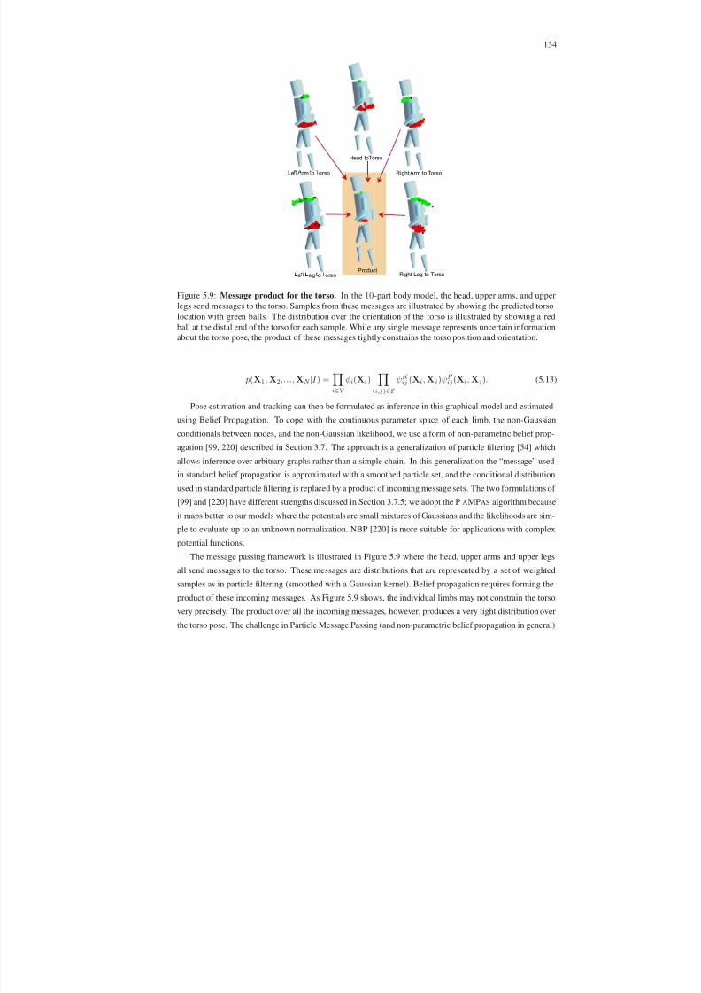
8/13/2019 Continuous-State Graphical Models for Object Localization, Pose Estimation and Tracking
http://slidepdf.com/reader/full/continuous-state-graphical-models-for-object-localization-pose-estimation 149/220
134
e eg o orso
Le rm o orso Right Arm to Torso
Right Leg to Torso
Head toTorso
Product
Figure 5.9: Message product for the torso. In the 10-part body model, the head, upper arms, and upper
legs send messages to the torso. Samples from these messages are illustrated by showing the predicted torso
location with green balls. The distribution over the orientation of the torso is illustrated by showing a red
ball at the distal end of the torso for each sample. While any single message represents uncertain information
about the torso pose, the product of these messages tightly constrains the torso position and orientation.
p(X1,X2,...,XN |I ) =i∈V
φi(Xi)
(i,j)∈E ψK ij (Xi,Xj)ψP ij(Xi,Xj). (5.13)
Pose estimation and tracking can then be formulated as inference in this graphical model and estimated
using Belief Propagation. To cope with the continuous parameter space of each limb, the non-Gaussian
conditionals between nodes, and the non-Gaussian likelihood, we use a form of non-parametric belief prop-
agation [99, 220] described in Section 3.7. The approach is a generalization of particle filtering [54] which
allows inference over arbitrary graphs rather than a simple chain. In this generalization the “message” used
in standard belief propagation is approximated with a smoothed particle set, and the conditional distribution
used in standard particle filtering is replaced by a product of incoming message sets. The two formulations of
[99] and [220] have different strengths discussed in Section 3.7.5; we adopt the P AMPAS algorithm because
it maps better to our models where the potentials are small mixtures of Gaussians and the likelihoods are sim-
ple to evaluate up to an unknown normalization. NBP [220] is more suitable for applications with complex
potential functions.
The message passing framework is illustrated in Figure 5.9 where the head, upper arms and upper legs
all send messages to the torso. These messages are distributions that are represented by a set of weighted
samples as in particle filtering (smoothed with a Gaussian kernel). Belief propagation requires forming the
product of these incoming messages. As Figure 5.9 shows, the individual limbs may not constrain the torso
very precisely. The product over all the incoming messages, however, produces a very tight distribution over
the torso pose. The challenge in Particle Message Passing (and non-parametric belief propagation in general)

8/13/2019 Continuous-State Graphical Models for Object Localization, Pose Estimation and Tracking
http://slidepdf.com/reader/full/continuous-state-graphical-models-for-object-localization-pose-estimation 150/220
135
is to compute the product of multiple such sampled distributions efficiently. If each sample is represented by
a small Gaussian kernel, then the explicit product of D messages each containing N kernels requires O(N D)
time to compute, which is impractical in most cases where D > 2. Hence, for D > 2 we use the Gibbs
sampler described in Section 3.7.1 (Algorithm 5) that can draw approximate and asymptotically unbiased
samples from the product in O(DN 2). For D
≤ 2 we compute the message product explicitly.
In PAMPAS the belief propagation messages are approximated using Monte-Carlo importance sampling.
This is achieved by sampling from the product of messages and then propagating these samples through
an appropriate potential function. Since in our loose-limbed body model formulation we have two types of
potential functions, ψK ij (Xi,Xj) and ψP ij(Xi,Xj) that have different representations, the messages in the
two cases will be different as well,
mK ij (Xj) =
ψK ij (Xi,Xj)φi(Xi)
k∈A(i)\j
mK ki(Xi)mP
ki(Xi)dXi (5.14)
mP ij(Xj) =
ψP ij(Xi,Xj)φi(Xi)
k∈A(i)
\j
mK ki(Xi)mP
ki(Xi)dXi (5.15)
where A(i) is the set of neighbors of node i and φi(Xi) is the local likelihood associated with node i.
Note that mK ij (Xj) is represented using a mixture of Gaussian kernel densities and mP
ij(Xj) by a mixture
of continuous unnormalized functions. These representations stem from the choice of potential functions
discussed in Sections 5.3.1 and 5.3.2 respectively. The stratified PAMPAS algorithm (see Algorithm 6) can
be modified to handle this case by choosing proper importance functions. In particular,
q (1)ij (Xi) =
k∈A(i)\j
mK ki(Xi) (5.16)
q
(2)
ij (Xi) = k∈A(i)
mK
ki(Xi) (5.17)
q (3)ij (Xi) = f (Xi). (5.18)
The messages, mK ij (Xj) and mP
ij(Xj), are hence generated by sampling from the above importance func-
tions, applying a proper re-weighting scheme, and propagating these weighted samples that intuitively ac-
count for distribution over Xi through a potential function ψK ij (Xi,Xj) or ψP ij(Xi,Xj) respectively. For
further details see Section 3.7.
Illustration of PAMPAS being utilized for pose estimation with 10-part loose-limbed body model can be
seen in Figure 5.10. In Figure 5.10 marginals are illustrated in terms of the most likely sample drawn from the
marginal, on the left, and the full distribution visualized by overlapping samples on the right. In all images
the dark and light green illustrate parts belonging to the left and right sides of the body respectively; yellow
illustrates coordinate frames for the torso and the head. One can clearly see how the marginals converge to
the desired solution within the first 5-6 iterations.
The basic algorithm outlined in Section 3.7 leaves open questions of (1) what proportions to use in the
stratified sampler, (2) how many particles to use for Monte Carlo approximation of each message and (3)
what order to use in updating the messages.

8/13/2019 Continuous-State Graphical Models for Object Localization, Pose Estimation and Tracking
http://slidepdf.com/reader/full/continuous-state-graphical-models-for-object-localization-pose-estimation 151/220
136
Camera: C1 Camera: C2
Most Likely Sample Full Distribution Most Likely Sample Full Distribution
I t
e r a t i o n : 1
I t e r a t i o n : 2
I t e r a t i o n : 3
I t e r a t i o n : 4
I t e r a t i o n : 5
• • • • • •
I t e r a t i o n : 7
• • • • • •
I t e r a t i o n : 9
Figure 5.10: Illustration of convergence of loose-limbed body model during pose estimation. Resulting
marginals for each limb estimated by PAMPAS are illustrated after 1-5, 7 and 9 message passing iterations.
As can be observed, marginals converge to a desired solution in roughly 5 iterations in this case, after which
point the marginals are refined without significantly affecting the mode of the marginal distribution. The error
curve as a function of PAMPAS iterations for this frame can be found in Figure 5.13 (Frame 450).

8/13/2019 Continuous-State Graphical Models for Object Localization, Pose Estimation and Tracking
http://slidepdf.com/reader/full/continuous-state-graphical-models-for-object-localization-pose-estimation 152/220
137
Implementation Details
Sampling Proportions. The stratified sampler we use, samples all the samples from q (3)ij (Xi) for the first
message passing iteration and then samples half of samples from q (1)ij (Xi) and half from q
(2)ij (Xi) for the
remaining iterations. We found the sampling from q (2)ij (Xi) sometimes lead to faster convergence, where as
sampling from q
(1)
ij (Xi) often leads to better results when the solution is close to convergence. Consequentlywe have also experimented with adapting sampling proportions, using an annealing schedule based on the
number of message passing iterations. The idea being, that while in the beginning where there is a large
uncertainty about the solution, we should sample equally from q (1)ij (Xi) and q
(2)ij (Xi), as the solutions starts
to converge (assuming it is converging with iterations of BP) we should sample more from q (1)ij (Xi). While
this proved to be useful in some instances, it also sometimes introduced biases particularly when the stra-
tum corresponding to the q (2)ij (Xi) was small. Hence, for simplicity, for all experiments here we use equal
sampling fractions for q (1)ij (Xi) and q
(2)ij (Xi).
Number of samples. The number of particles/samples used to approximate messages has a significant effect
on the runtime of the algorithm. While the basic Particle Message Passing algorithm assumes that all mes-
sages are approximated using the same number of N samples, we found this to be sub-optimal. In particular,
we found that messages going out of the nodes that are highly connected ( e.g. torso) are often more compact
and require fewer samples to represent adequately; alternatively, messages that correspond to outer nodes in
the graph, that have fewer connections, need more samples to be adequately represented. Hence, we derived
an ad-hoc adaptive procedure for the number of samples required to represent the massage based on the de-
gree of the node sending the message. In particular, for all experiments we used the following number of
samples to approximate messages sent from node i:
Node i # of samples Mixtures in potential Message representation
torso 50 Kinematic: 4 mK ij (Xj) = mixture of 201 Gaussian kernels
Penetration: 1 mP ij(Xj) = 1 - mixture of 50 Gaussian kernels
head, shins, 200 Kinematic: 4 mK ij (Xj) = mixture of 801 Gaussian kernels
upper arms Penetration: 1 mP ij(Xj) = 1 - mixture of 200 Gaussian kernels
calfs, 800 Kinematic: 4 mK ij (Xj) = mixture of 2401 Gaussian kernels
lower arms Penetration: 1 mP ij(Xj) = 1 - mixture of 800 Gaussian kernels
(In addition for 15-part model)
hands, feet 800 Kinematic: 4 mK ij (Xj) = mixture of 2401 Gaussian kernels
Penetration: 1 mP ij(Xj) = 1 - mixture of 800 Gaussian kernels
Note that penetration messages due to their non-Gaussian form are simply treated in the PAMPAS framework
as continuous functions. Deriving automatically the number of samples required for each message would
clearly be of benefit, however, this is hard to do in general, since the number of samples must be a function
of the overall graph topology, importance functions employed for Monte Carlo integration, and distributions
of all involved variables.
Message passing schedule. As mentioned in Section 3.7 in order to perform inference in a loopy graphical
model, one needs to define the message update schedule. We use a fixed message update schedule that sends
messages from the outer extremities inward toward the torso and then back out (from the torso to outer

8/13/2019 Continuous-State Graphical Models for Object Localization, Pose Estimation and Tracking
http://slidepdf.com/reader/full/continuous-state-graphical-models-for-object-localization-pose-estimation 153/220
138
extremities). We also first propagate the kinematic messages and then the penetration messages. For pose
estimation we run PAMPAS for 10 message passing iterations per frame (with convergence often achieved
in 5–6 iterations), and for tracking (that will be discussed in the next section) for only 2 message passing
iterations per frame. The underlying assumption being that in the tracking framework the pose is likely to be
relatively well constrained by the estimate from the previous time frame, and hence PAMPAS often converges
faster.
5.6.1 Tracking
Thus far we have only addressed the problem of pose estimation and have not dealt with incorporating tem-
poral consistency into our model. This is partly due to the fact that ability to automatically estimate the pose
is one of the key benefits of the loose-limbed body model. However, our model can also incorporate temporal
consistency. Temporal consistency (or tracking) can be performed in at least two different ways within our
framework.
Tracking using a spatio-temporal model
The most direct way of extending the proposed pose estimation framework to tracking, is by replicating
and chaining the spatial loose-limbed body model across time. This methodology was already introduced
in somewhat different context in Chapter 4. The new spatio-temporal graphical model requires additional
temporal constraints between limbs at time t − 1 and t, that we denote by ψT (Xi,t−1,Xi,t). Typically a
single Gaussian potential is sufficient to model these temporal constraints. For example,
ψT (Xi,t−1,Xi,t) = N (Xi,t −Xi,t−1|0, ΛT ), (5.19)
is equivalent to a zero velocity assumption. With this type of temporal constraint, inference can be performed
as before using Particle Message Passing in either batch or sliding window fashion. We have explored this
alternative in [197]. A similar approach has also been discussed in the context of generic object tracking in
Chapter 4.
The benefit of this type of spatio-temporal model is that temporal consistency is well maintained, the
disadvantage is the additional computational complexity incurred by this more complex model. In addition,
if tracking fails, the spatio-temporal model is often harder to re-initialize, because of the tight coupling to the
pose at the previous time instants.
Tracking using importance sampling
An alternative approach, that we take in this chapter, is to propagate the temporal consistency via an im-
portance function. This approach does not alter the model already introduced, and hence does not require
additional computation. In essence, it assumes that we are solving the pose estimation problem at every
frame, and the pose from the previous time step is only used as an initialization (or guess) for where to start
the inference at the next frame. As such, this approach is well suited for re-initialization if the pose estimate
at the previous timeframe is wrong. The disadvantage is that temporal consistency is only loosely propagated,
and the results often exhibit interframe jitter.
In particular, we can define another importance function,

8/13/2019 Continuous-State Graphical Models for Object Localization, Pose Estimation and Tracking
http://slidepdf.com/reader/full/continuous-state-graphical-models-for-object-localization-pose-estimation 154/220
139
q (4)ij (Xi,t) = N (Xi,t|Xi,t−1, ΛT ). (5.20)
Sampling from this importance function places the samples in the vicinity of the solution obtained at the
previous time step. This is then refined using the observations from the current frame and the message
passing. Altering the fraction of samples that come from the different importance functions in the stratifiedsampling will have an affect on the diversity of poses considered at any given time instant. Ultimately the
optimal importance sampling procedure would have to rely on knowledge of the scene and human postures
considered. For experiments presented in this chapter, we make no such assumptions and use a simple generic
importance sampling scheme discussed previously.
5.7 Experiments and Evaluation
5.7.1 HumanEva-I Dataset
To test performance of our articulated pose estimation and tracking approach we collected the novel dataset
10
that we call HUMANEVA-I. In HUMANEVA-I we simultaneously captured 3D motion and mutioccular video
using a calibrated marker-based motion capture system11 and multiple high-speed video cameras. We col-
lected video data using 3 color and 4 greyscale cameras at 60 Hz. The video and motion capture streams
were synchronized in software using a direct optimization method. The H UMANEVA-I database consists of 4
subjects performing a set of 6 predefined actions three times (twice with video and motion capture, and once
with motion capture alone). The dataset is partitioned into training, validation and testing sub-sets. A more
detailed description of the dataset, data collection and processing can be found in [194].
To simultaneously capture video and motion information, our subjects wore natural clothing (as opposed
to motion capture suits which are often used for pure motion capture sessions) on which reflective markers
were attached using transparent adhesive tape. Our motivation was to obtain natural looking image data thatcontains all the complexity posed by moving clothing. One negative outcome of this is that the markers
tend to move more than they would with a tight-fitting motion capture suit. As result, our ground truth
motion capture data may not always be as accurate as that obtained by more traditional methods; we felt that
the trade-off of accuracy for realism here was acceptable. We have applied minimal post-processing to the
motion capture data, steering away from the use of complex software packages ( e.g. Motion Builder) that
may introduce biases or alter the motion data in the process.
5.7.2 Evaluation Metric
Various evaluation metrics have been proposed for human motion tracking and pose estimation. For example,
a number of papers [1, 2, 3, 4, 166, 189, 206] have suggested using joint-angle distance as the error measure.
This measure, however, assumes a particular parameterization of the human body and cannot be used to com-
pare methods where the body models have different degrees of freedom or have different parameterizations
10Dataset is available from http://vision.cs.brown.edu/humaneva/.
11We collected motion capture data using a commercial motion capture (MoCap) system from ViconPeak (http://www.vicon.
com/). The ViconPeak MoCap system is an industry standard for optical marker-based motion capture and has been successfully
employed in a variety of entertainment applications for over 10 years. The system uses reflective markers and six 1M-pixel cameras to
recover the 3D position of the markers on the body.

8/13/2019 Continuous-State Graphical Models for Object Localization, Pose Estimation and Tracking
http://slidepdf.com/reader/full/continuous-state-graphical-models-for-object-localization-pose-estimation 155/220
140
Figure 5.11: Virtual marker-based evaluation metric. We define an evaluation metric based on the average
distance between a set of 15 virtual markers corresponding to the 3D joint positions and limb ends illustrated
in the figure above.
of the joint angles.
We propose an error measure based on a sparse set of virtual markers that correspond to the locations of joints12 and limb endpoints (see Figure 5.11). This metric is not sensitive to parameterization of the skeletal
structure of the body and can easily be derived from most body representations, allowing easy comparison
across many approaches. This error metric was first introduced for 3D pose estimation and tracking by us in
[197] and later extended in [14]. It has since been also adopted by others for 3D tracking [131] and for 2D
pose estimation evaluation in [122, 196].
Assuming that we can represent the pose of the body using K = 15 virtual markers, we can write the state
of the bodyas Xmrk = p1, p2,...,pK , where pk ∈ R3 is the positionof the marker k in theworld13. Notice,
that converting from any standard representation of the body pose to Xmrk is trivial. In particular, to convert
from our redundant representation of the bodyX = X1,X2,...,XN toXmrk all we need to do, is for every
marker (except for the markers corresponding to the limb ends) compute an average of the proximal and distalends14 of the two limbs connected at the corresponding joint. For example, computing the virtual marker
position corresponding to the left knee joint, pleft knee = ||H (Xleft shin)[0, 0, lleft shin]T − xleft calf ||1/2,
where H (Xleft shin) is as before a 3D homogeneous object-to-world transformation matrix; lleft shin is the
length of the left shin. In other words, H (Xleft shin)[0, 0, lleft shin]T is simply a distal endpoint of the left
shin and xleft calf is the proximal endpoint of the left calf. The error in the overall estimated pose Xmrk
to the ground truth pose Xmrk can then be expressed as the average absolute distance between individual
markers,
Error(Xmrk, Xmrk) =
K
k=0
|| pk − ˆ pk||K
. (5.21)
Since the position of virtual markers is defined in the global coordinate frame the error will have a physical
12The ground truth location of joints was computed from the motion capture data using the Plug-in Gait software module from
ViconPeak (http://www.vicon.com/ ).
13Notice that pk can also be ∈ R2 if a 2D body model is used. This is the error measure that will be employed in the next chapter.
14This assumes that both proximal and distal markers correspond to the joint center. Alternatively, if this is not the c ase, there will be
a constant offset between the proximal and/or distal ends of the limb and the required joint marker. This offset can typically be solved
for in a least-squared sense using regression.

8/13/2019 Continuous-State Graphical Models for Object Localization, Pose Estimation and Tracking
http://slidepdf.com/reader/full/continuous-state-graphical-models-for-object-localization-pose-estimation 156/220
141
34 (mm) 65 (mm) 108 (mm) 175 (mm)
80 (mm) 120 (mm) Error
Accurate
Acceptable
Inaccurate/Wrong
Figure 5.12: Evaluation metric illustration. This figure visually illustratesthe range of errors corresponding
to the virtual marker-based metric introduced. Typically an error of < 80 (mm) corresponds to accurate pose
estimation and an error between 80–120 (mm) to a reasonable pose. As can be seen from the figure with an
error of 108 (mm) the body is vertically shifted down and the arms are less than perfect, but the overall pose
is still reasonable. Typically error > 120 (mm) corresponds to wrong or inaccurate poses as illustrated.
meaning and is expressed in (mm). Lower error will correspond to poses that more closely match the ground
truth motion capture data. Since the proposed error function averages error over a set of limbs, the exact
meaning of the error will depend on the distribution of errors across the body parts at a given frame. The
same is true for most other metrics we have found in the literature. In other words, the same quantitative error
may be due to either a single joint being off by a considerable amount, or by all the joints being off by small
amount. Our approach, due to the nature of the model and inference, tries to distribute error across limbs. In
our experience, errors of under 80 (mm) correspond to accurate poses, 80–120 (mm) typically correspond to
poses of acceptable accuracy, and errors of > 120 (mm) typically correspond to wrong or inaccurate poses.
By acceptable accuracy we mean that all parts are recovered, but there may be misalignments at the joints (see
Figure 5.12) or slight global vertical shift of the body. To compute performance over a temporal sequence
(for tracking), we average the error over all the frames in the sequence and report the mean and standard
deviation.
5.7.3 Pose Estimation
Figures 5.13–5.17 show the automatic pose estimation of the 3D body model using bottom-up part detectors.
The approach is tested on a total of 198 frames; 128 frames using a 10-part model and 70 frames using a 15-
part loose-limbed body model. Note that we use only detectors for the head, and outermost extremities, which
for the 10-part model means upper arms and calfs; for the 15-part model hands and feet. These detectors are
very noisy and at best can only give a rough position of the part in space. They are unable to differentiate left
and right sides of the body, estimate the twist, or even differentiate the direction in which the limb is pointing.
For body parts with no associated bottom-up detectors, the initial distributions are assumed to be uniform
over the entire state space. After several iterations of belief propagation, the algorithm “finds” the limbs and
has a reasonable distribution over the limbs poses. Notice that while we run PAMPAS for 10 message passing
iterations to ensure convergence, the solution often settles after 5–6 iterations.

8/13/2019 Continuous-State Graphical Models for Object Localization, Pose Estimation and Tracking
http://slidepdf.com/reader/full/continuous-state-graphical-models-for-object-localization-pose-estimation 157/220

8/13/2019 Continuous-State Graphical Models for Object Localization, Pose Estimation and Tracking
http://slidepdf.com/reader/full/continuous-state-graphical-models-for-object-localization-pose-estimation 158/220

8/13/2019 Continuous-State Graphical Models for Object Localization, Pose Estimation and Tracking
http://slidepdf.com/reader/full/continuous-state-graphical-models-for-object-localization-pose-estimation 159/220
144
Camera: C1 Camera: C2 Camera: C3
F r a m e 1 1 0
1 2 3 4 5 6 7 8 9 1040
50
60
70
80
90
100
Particle Message Passing (NBP) Iteration
E
r r o r i n ( m m )
F r a m e 1 3 0
1 2 3 4 5 6 7 8 9 1030
40
50
60
70
80
90
100
110
120
130
Particle Message Passing (NBP) Iteration
E r r o r i n ( m m )
F r a m e 2 3 0
1 2 3 4 5 6 7 8 9 1040
60
80
100
120
140
160
Particle Message Passing (NBP) Iteration
E r r o r i n ( m m )
F r a m e 2 7 0
1 2 3 4 5 6 7 8 9 1040
45
50
55
60
65
70
75
80
85
90
Particle Message Passing (NBP) Iteration
E r r o r i n ( m m )
F r a
m e 3 3 0
1 2 3 4 5 6 7 8 9 100
50
100
150
200
250
300
Particle Message Passing (NBP) Iteration
E r r o r i n ( m m )
0 50 100 150 200 250 3000
2
4
6
8
10
12
14
16
18
Error in (mm) After 10 Iterations of PaMPas
N u m b e r o f F r a m e s
1 2 3 4 5 6 7 8 9 1080
90
100
110
120
130
140
150
160
Particle Message Passing (NBP) Iteration
A v e r a g e E r r o r i n ( m m )Dataset: HumanEva-I
Partision: Validation
Subject: S1
Action: Jog
# frames: 31
Figure 5.14: Pose estimation using 10-part loose-limbed body model. Results of pose estimation from a
single multioccular frame are shown for a number of frames from HumanEva-I dataset. Top five rows show
the final result in terms of most likely sample from the marginal for each part after 10 iterations of PAMPAS.The results are projected into 3 synchronized views for clarity (7 views were used for inference). The right
column of the first five rows shows the error as a function of message passing iterations for respective frames.
Notice that typically the error decreases sharply for the first 4–5 iterations and then stays relatively low with
minor variations that are due to sampling. The last row illustrates performance over all (31) frames tested for
the sequence (every 10-th frame was selected). As can be seen from bar plot, the pose was estimated in the
pose with low error. The error as a function of message passing iterations averaged over all frames is shown
in the bottom right corner of the figure.

8/13/2019 Continuous-State Graphical Models for Object Localization, Pose Estimation and Tracking
http://slidepdf.com/reader/full/continuous-state-graphical-models-for-object-localization-pose-estimation 160/220
145
Camera: C1 Camera: C2 Camera: C3
F r a
m e 8 0
1 2 3 4 5 6 7 8 9 100
50
100
150
200
250
300
Particle Message Passing (NBP) Iteration
E
r r o r i n ( m m )
F r a m e 1 1 0
1 2 3 4 5 6 7 8 9 100
50
100
150
200
250
300
Particle Message Passing (NBP) Iteration
E r r o r i n ( m m )
F r a m e 1 4 0
1 2 3 4 5 6 7 8 9 100
50
100
150
200
250
300
Particle Message Passing (NBP) Iteration
E r r o r i n ( m m )
F r a m e 1 6 0
1 2 3 4 5 6 7 8 9 100
50
100
150
200
250
300
350
Particle Message Passing (NBP) Iteration
E r r o r i n ( m m )
F r a
m e 2 3 0
1 2 3 4 5 6 7 8 9 100
50
100
150
200
250
300
350
400
Particle Message Passing (NBP) Iteration
E r r o r i n ( m m )
0 50 100 150 200 250 300 3500
1
2
3
4
5
6
7
8
9
10
Error in (mm) After 10 Iterations of PaMPas
N u m b e r o f F r a m e s
1 2 3 4 5 6 7 8 9 10120
140
160
180
200
220
240
260
280
Particle Message Passing (NBP) Iteration
A v e r a g e E r r o r i n ( m m )Dataset: HumanEva-I
Partision: Validation
Subject: S1
Action: Jog
# frames: 31
Figure 5.15: Pose estimation using 15-part loose-limbed body model. Results of pose estimation from a
single multioccular frame are shown for a number of frames from HumanEva-I dataset. Top five rows show
the final result in terms of most likely sample from the marginal for each part after 10 iterations of PAMPAS.The results are projected into 3 synchronized views for clarity (7 views were used for inference). The right
column of the first five rows shows the error as a function of message passing iterations for respective frames.
Notice that typically the error decreases sharply for the first 4–5 iterations and then stays relatively low with
minor variations that are due to sampling. The last row illustrates performance over all (31) frames tested
for the sequence (every 10-th frame was selected). As can be seen from bar plot, the pose was estimated in
most frames with low error. The error as a function of message passing iterations averaged over all frames is
shown in the bottom right corner of the figure.

8/13/2019 Continuous-State Graphical Models for Object Localization, Pose Estimation and Tracking
http://slidepdf.com/reader/full/continuous-state-graphical-models-for-object-localization-pose-estimation 161/220
146
Camera: C1 Camera: C2 Camera: C3
F r a m e 1 3 0
1 2 3 4 5 6 7 8 9 1040
50
60
70
80
90
100
110
120
130
Particle Message Passing (NBP) Iteration
E
r r o r i n ( m m )
F r a m e 2 1 0
1 2 3 4 5 6 7 8 9 1035
40
45
50
55
60
65
70
75
Particle Message Passing (NBP) Iteration
E r r o r i n ( m m )
F r a m e 2 2 0
1 2 3 4 5 6 7 8 9 1030
40
50
60
70
80
90
100
110
120
Particle Message Passing (NBP) Iteration
E r r o r i n ( m m )
F r a m e 2 6 0
1 2 3 4 5 6 7 8 9 1040
60
80
100
120
140
160
180
200
220
240
Particle Message Passing (NBP) Iteration
E r r o r i n ( m m )
F r a
m e 3 3 0
1 2 3 4 5 6 7 8 9 1020
40
60
80
100
120
140
160
180
200
Particle Message Passing (NBP) Iteration
E r r o r i n ( m m )
0 50 100 150 200 250 300 350 4000
1
2
3
4
5
6
7
8
9
10
Error in (mm) After 10 Iterations of PaMPas
N u m b e r o f F r a m e s
1 2 3 4 5 6 7 8 9 10160
170
180
190
200
210
220
Particle Message Passing (NBP) Iteration
A v e r a g e E r r o r i n ( m m )Dataset: HumanEva-I
Partision: Validation
Subject: S2
Action: Walking
# frames: 39
Figure 5.16: Pose estimation using 10-part loose-limbed body model. Results of pose estimation from a
single multioccular frame are shown for a number of frames from HumanEva-I dataset. Top five rows show
the final result in terms of most likely sample from the marginal for each part after 10 iterations of PAMPAS.The results are projected into 3 synchronized views for clarity (7 views were used for inference). The right
column of the first five rows shows the error as a function of message passing iterations for respective frames.
Notice that typically the error decreases sharply for the first 4–5 iterations and then stays relatively low with
minor variations that are due to sampling. The last row illustrates performance over all (39) frames tested
for the sequence (every 10-th frame was selected). As can be seen from bar plot, the pose was estimated in
most frames with low error. The error as a function of message passing iterations averaged over all frames is
shown in the bottom right corner of the figure.

8/13/2019 Continuous-State Graphical Models for Object Localization, Pose Estimation and Tracking
http://slidepdf.com/reader/full/continuous-state-graphical-models-for-object-localization-pose-estimation 162/220
147
Camera: C1 Camera: C2 Camera: C3
F r a
m e 4 0
1 2 3 4 5 6 7 8 9 100
50
100
150
200
250
300
350
Particle Message Passing (NBP) Iteration
E
r r o r i n ( m m )
F r a m e 5 0
1 2 3 4 5 6 7 8 9 1020
40
60
80
100
120
140
160
180
200
220
Particle Message Passing (NBP) Iteration
E r r o r i n ( m m )
F r a m e 2 0 0
1 2 3 4 5 6 7 8 9 100
50
100
150
200
250
300
Particle Message Passing (NBP) Iteration
E r r o r i n ( m m )
F r a m e 3 1 0
1 2 3 4 5 6 7 8 9 1020
40
60
80
100
120
140
160
180
200
Particle Message Passing (NBP) Iteration
E r r o r i n ( m m )
F r a
m e 3 9 0
1 2 3 4 5 6 7 8 9 1040
60
80
100
120
140
160
180
200
Particle Message Passing (NBP) Iteration
E r r o r i n ( m m )
0 100 200 300 400 500 6000
2
4
6
8
10
12
14
16
18
Error in (mm) After 10 Iterations of PaMPas
N u m b e r o f F r a m e s
1 2 3 4 5 6 7 8 9 10140
160
180
200
220
240
260
Particle Message Passing (NBP) Iteration
A v e r a g e E r r o r i n ( m m )Dataset: HumanEva-I
Partision: Validation
Subject: S2
Action: Walking
# frames: 39
Figure 5.17: Pose estimation using 15-part loose-limbed body model. Results of pose estimation from a
single multioccular frame are shown for a number of frames from HumanEva-I dataset. Top five rows show
the final result in terms of most likely sample from the marginal for each part after 10 iterations of PAMPAS.The results are projected into 3 synchronized views for clarity (7 views were used for inference). The right
column of the first five rows shows the error as a function of message passing iterations for respective frames.
Notice that typically the error decreases sharply for the first 4–5 iterations and then stays relatively low with
minor variations that are due to sampling. The last row illustrates performance over all (39) frames tested
for the sequence (every 10-th frame was selected). As can be seen from bar plot, the pose was estimated in
most frames with low error. The error as a function of message passing iterations averaged over all frames is
shown in the bottom right corner of the figure.

8/13/2019 Continuous-State Graphical Models for Object Localization, Pose Estimation and Tracking
http://slidepdf.com/reader/full/continuous-state-graphical-models-for-object-localization-pose-estimation 163/220
148
Subject S2 S1 S1 S2
Action Walking Walking Jog Walking
Frames 400 391 201 213
Model 10-part 15-part 15-part 15-part
Mean Error (mm) 74 59 77 69
Standard deviation of Error (mm) 9.95 25.2 20.2 18.8
Average for the model (mm) 74 66Standard deviation for the model (mm) 9.95 23.5
Table 5.3: Summary of tracking performance using loose-limbed body model. More detailed results can
be found in Figures 5.18–5.21.
model. The average performance over the sequence ranges between 59–77 (mm) in all cases (see summary
of results in Table 5.3). Also, notice that the approach quickly recovers when infrequent miss-tracking occurs
(see Frame 78 in Figure 5.18).
5.7.5 Comparison with Annealed Particle Filter
In previous section we explored performance of the loose-limbed body model in the context of tracking. In
this section, we compare the results obtained by our approach to a relatively standard tracking algorithm,
Annealed Particle Filter (APF) (see Section 2.8 for more detailed description). In particular, we make use of
the APF algorithm implemented15 and tested by Balan et al. in [14]. In our comparison, Annealed Particle
Filter performs inference over kinematic tree body model with 15 parts, comparable to our 15-part loose-
limbed body model; the resulting state-space parameterization of the pose is ∈ R40 , corresponding to global
position and orientation of the torso in 3D and 36 joint angles. Consequently, the implementation of APF we
employ is also using comparable likelihood function that incorporates silhouette and edge information (see
[14] for details). Unlike the original APF algorithm proposed by Deutscher et al. [52], the variant of [14] isalso able to incorporate the temporal and structural priors, that ensure that parts do not penetrate each other
and that joints are within the allowable limits. In Figure 5.22 we compare our model with three variants of
APF algorithm: generic APF with interpenetration constraints and very generic joint limits with ( i) 250 and
(ii) 500 particles, and (iii) an APF algorithm that in addition encodes action-specific joint limits and temporal
prior. In all cases Annealed Particle Filter requires an initial pose at the first frame to bootstrap the inference;
this was obtained from ground truth motion capture data.
Loose-limbed body model in both sequences outperforms the generic APF algorithms (consequently,
the number of particles seems to play little significance in the overall performance of APF) and performs
comparably to the action-specific APF variant (see Figure 5.22). In all cases, however, the variance for the
estimates obtained using APF are lower than those obtained using our loose-limbed body model. This is notsurprising, considering the nature of inference employed in the loose-limbed body model, where the pose
at the previous time instant is simply a proposal for inference at the next time frame. While this type of
inference is beneficial in that it allows easy recovery from intermittent failures, the pose estimation that is
inherently incorporated at every frame also tends to produce noisier results when such failures are not present.
15Implementation of APF is curtesy of Alexandru Balan and is freely distributed from http://www.cs.brown.edu/˜alb/
software.htm.

8/13/2019 Continuous-State Graphical Models for Object Localization, Pose Estimation and Tracking
http://slidepdf.com/reader/full/continuous-state-graphical-models-for-object-localization-pose-estimation 164/220
149
Frame: 78 Frame: 156 Frame: 234 Frame: 312
C a m e r a : C 1
C a m e r a : C 2
C a m e r a : C 3
50 100 150 200 250 300 3500
20
40
60
80
100
120
140
160
180
200
Frame #
E r r o r i n ( m m )
Dataset: HumanEva-I
0
10
20
30
40
50
60
70
80
90
Virtual Marker
M e a n E r r o r ( m m )
t o r s o P r o x i m a l
t o r s o D i s t a l
u p p e r L L e g P r o x i m a l
u p p e r L L e g D i s t a l
l o w e r L L e g P r o x i m a l
l o w e r L L e g D i s t a l
u p p e r R L e g P r o x i m a l
u p p e r R L e g D i s t a l
l o w e r R L e g P r o x i m a l
l o w e r R L e g D i s t a l
u p p e r L A r m P r o x i m a l
u p p e r L A r m D i s t a l
l o w e r L A r m P r o x i m a l
l o w e r L A r m D i s t a l
u p p e r R A r m P r o x i m a l
u p p e r R A r m D i s t a l
l o w e r R A r m P r o x i m a l
l o w e r R A r m D i s t a l
h e a d P r o x i m a l
h e a d D i s t a l
0
10
20
30
40
50
60
70
80
90
Virtual Marker
S t a n d a r d D e v i a t i o n o f E r r o r ( m m )
t o r s o P r o x i m a l
t o r s o D i s t a l
u p p e r L L e g P r o x i m a l
u p p e r L L e g D i s t a l
l o w e r L L e g P r o x i m a l
l o w e r L L e g D i s t a l
u p p e r R L e g P r o x i m a l
u p p e r R L e g D i s t a l
l o w e r R L e g P r o x i m a l
l o w e r R L e g D i s t a l
u p p e r L A r m P r o x i m a l
u p p e r L A r m D i s t a l
l o w e r L A r m P r o x i m a l
l o w e r L A r m D i s t a l
u p p e r R A r m P r o x i m a l
u p p e r R A r m D i s t a l
l o w e r R A r m P r o x i m a l
l o w e r R A r m D i s t a l
h e a d P r o x i m a l
h e a d D i s t a l
Partision: Validation
Subject: S1
Action: Walking
# frames: 391
Figure 5.18: Tracking using 15-part loose-limbed body model. Results of tracking in a multioccular
sequence from the HumanEva-I dataset are shown for a number of frames. Top three rows show the final
result in terms of most likely sample from the marginal for each part after 2 iterations of PAMPAS. The
results are projected into 3 synchronized views for clarity (7 views were used for inference). The figure in
the second to last row shows per frame error (in blue) for all 390 frames used for testing. The mean error
computed over the entire sequence and ±2σ are shown in solid and dashed magenta respectively. Frames
selected automatically and temporally equidistantly to visually illustrate performance (top three rows), are
designated by green circles on the graph. The last row illustrates an alternative analysis of error by showing
statistics for individual virtual markers, with mean on the left and standard deviation on the right, averaged
over the entire sequence. Notice that the approach successfully recovers from the miss-tracking that is starting
to present itself at frame 78. We believe that the source of the tracking failure here is caused by the ambiguity
in the image evidence; self-occlusions of the body under the particular placement of the cameras with respect
to the observed pose make it hard to disambiguate true and recovered pose based on image evidence alone.

8/13/2019 Continuous-State Graphical Models for Object Localization, Pose Estimation and Tracking
http://slidepdf.com/reader/full/continuous-state-graphical-models-for-object-localization-pose-estimation 165/220
150
Frame: 40 Frame: 80 Frame: 120 Frame: 160
C a m e r a : C 1
C a m e r a : C 2
C a m e r a : C 3
20 40 60 80 100 120 140 160 180 2000
20
40
60
80
100
120
140
160
180
200
Frame #
E r r o r i n ( m m )
Dataset: HumanEva-I
0
50
100
150
Virtual Marker
M e a n E r r o r ( m m )
t o r s o P r o x i m a l
t o r s o D i s t a l
u p p e r L L e g P r o x i m a l
u p p e r L L e g D i s t a l
l o w e r L L e g P r o x i m a l
l o w e r L L e g D i s t a l
u p p e r R L e g P r o x i m a l
u p p e r R L e g D i s t a l
l o w e r R L e g P r o x i m a l
l o w e r R L e g D i s t a l
u p p e r L A r m P r o x i m a l
u p p e r L A r m D i s t a l
l o w e r L A r m P r o x i m a l
l o w e r L A r m D i s t a l
u p p e r R A r m P r o x i m a l
u p p e r R A r m D i s t a l
l o w e r R A r m P r o x i m a l
l o w e r R A r m D i s t a l
h e a d P r o x i m a l
h e a d D i s t a l
0
20
40
60
80
100
Virtual Marker
S t a n d a r d D e v i a t i o n o f E r r o r ( m m )
t o r s o P r o x i m a l
t o r s o D i s t a l
u p p e r L L e g P r o x i m a l
u p p e r L L e g D i s t a l
l o w e r L L e g P r o x i m a l
l o w e r L L e g D i s t a l
u p p e r R L e g P r o x i m a l
u p p e r R L e g D i s t a l
l o w e r R L e g P r o x i m a l
l o w e r R L e g D i s t a l
u p p e r L A r m P r o x i m a l
u p p e r L A r m D i s t a l
l o w e r L A r m P r o x i m a l
l o w e r L A r m D i s t a l
u p p e r R A r m P r o x i m a l
u p p e r R A r m D i s t a l
l o w e r R A r m P r o x i m a l
l o w e r R A r m D i s t a l
h e a d P r o x i m a l
h e a d D i s t a l
Partision: Validation
Subject: S1
Action: Jog
# frames: 201
Figure 5.19: Tracking using 15-part loose-limbed body model. Results of tracking in a multioccular
sequence from the HumanEva-I dataset are shown for a number of frames. Top three rows show the final
result in terms of most likely sample from the marginal for each part after 2 iterations of PAMPAS. The
results are projected into 3 synchronized views for clarity (7 views were used for inference). The figure in
the second to last row shows per frame error (in blue) for all 201 frames used for testing. The mean error
computed over the entire sequence and ±2σ are shown in solid and dashed magenta respectively. Frames
selected automatically and temporally equidistantly to visually illustrate performance (top three rows), are
designated by green circles on the graph. The last row illustrates an alternative analysis of error by showing
statistics for individual virtual markers, with mean on the left and standard deviation on the right, averaged
over the entire sequence.

8/13/2019 Continuous-State Graphical Models for Object Localization, Pose Estimation and Tracking
http://slidepdf.com/reader/full/continuous-state-graphical-models-for-object-localization-pose-estimation 166/220
151
Frame: 80 Frame: 159 Frame: 238 Frame: 317
C a m e r a : C 1
C a m e r a : C 2
C a m e r a : C 3
50 100 150 200 250 300 350 4000
20
40
60
80
100
120
140
160
180
200
Frame #
E r r o r i n ( m m )
Dataset: HumanEva-I
0
10
20
30
40
50
60
70
80
90
Virtual Marker
M e a n E r r o r ( m m )
t o r s o P r o x i m a l
t o r s o D i s t a l
u p p e r L L e g P r o x i m a l
u p p e r L L e g D i s t a l
l o w e r L L e g P r o x i m a l
l o w e r L L e g D i s t a l
u p p e r R L e g P r o x i m a l
u p p e r R L e g D i s t a l
l o w e r R L e g P r o x i m a l
l o w e r R L e g D i s t a l
u p p e r L A r m P r o x i m a l
u p p e r L A r m D i s t a l
l o w e r L A r m P r o x i m a l
l o w e r L A r m D i s t a l
u p p e r R A r m P r o x i m a l
u p p e r R A r m D i s t a l
l o w e r R A r m P r o x i m a l
l o w e r R A r m D i s t a l
h e a d P r o x i m a l
h e a d D i s t a l
0
5
10
15
20
25
30
Virtual Marker
S t a n d a r d D e v i a t i o n o f E r r o r ( m m )
t o r s o P r o x i m a l
t o r s o D i s t a l
u p p e r L L e g P r o x i m a l
u p p e r L L e g D i s t a l
l o w e r L L e g P r o x i m a l
l o w e r L L e g D i s t a l
u p p e r R L e g P r o x i m a l
u p p e r R L e g D i s t a l
l o w e r R L e g P r o x i m a l
l o w e r R L e g D i s t a l
u p p e r L A r m P r o x i m a l
u p p e r L A r m D i s t a l
l o w e r L A r m P r o x i m a l
l o w e r L A r m D i s t a l
u p p e r R A r m P r o x i m a l
u p p e r R A r m D i s t a l
l o w e r R A r m P r o x i m a l
l o w e r R A r m D i s t a l
h e a d P r o x i m a l
h e a d D i s t a l
Partision: Validation
Subject: S2
Action: Walking
# frames: 400
Figure 5.20: Tracking using 10-part loose-limbed body model. Results of tracking in a multioccular
sequence from the HumanEva-I dataset are shown for a number of frames. Top three rows show the final
result in terms of most likely sample from the marginal for each part after 2 iterations of PAMPAS. The
results are projected into 3 synchronized views for clarity (7 views were used for inference). The figure in
the second to last row shows per frame error (in blue) for all 400 frames used for testing. The mean error
computed over the entire sequence and ±2σ are shown in solid and dashed magenta respectively. Frames
selected automatically and temporally equidistantly to visually illustrate performance (top three rows), are
designated by green circles on the graph. The last row illustrates an alternative analysis of error by showing
statistics for individual virtual markers, with mean on the left and standard deviation on the right, averaged
over the entire sequence.

8/13/2019 Continuous-State Graphical Models for Object Localization, Pose Estimation and Tracking
http://slidepdf.com/reader/full/continuous-state-graphical-models-for-object-localization-pose-estimation 167/220
152
Frame: 42 Frame: 84 Frame: 126 Frame: 168
C a m e r a : C 1
C a m e r a : C 2
C a m e r a : C 3
20 40 60 80 100 120 140 160 180 2000
20
40
60
80
100
120
140
160
180
200
Frame #
E r r o r i n ( m m )
Dataset: HumanEva-I
0
10
20
30
40
50
60
70
80
90
Virtual Marker
M e a n E r r o r ( m m )
t o r s o P r o x i m a l
t o r s o D i s t a l
u p p e r L L e g P r o x i m a l
u p p e r L L e g D i s t a l
l o w e r L L e g P r o x i m a l
l o w e r L L e g D i s t a l
u p p e r R L e g P r o x i m a l
u p p e r R L e g D i s t a l
l o w e r R L e g P r o x i m a l
l o w e r R L e g D i s t a l
u p p e r L A r m P r o x i m a l
u p p e r L A r m D i s t a l
l o w e r L A r m P r o x i m a l
l o w e r L A r m D i s t a l
u p p e r R A r m P r o x i m a l
u p p e r R A r m D i s t a l
l o w e r R A r m P r o x i m a l
l o w e r R A r m D i s t a l
h e a d P r o x i m a l
h e a d D i s t a l
0
10
20
30
40
50
60
70
80
Virtual Marker
S t a n d a r d D e v i a t i o n o f E r r o r ( m m )
t o r s o P r o x i m a l
t o r s o D i s t a l
u p p e r L L e g P r o x i m a l
u p p e r L L e g D i s t a l
l o w e r L L e g P r o x i m a l
l o w e r L L e g D i s t a l
u p p e r R L e g P r o x i m a l
u p p e r R L e g D i s t a l
l o w e r R L e g P r o x i m a l
l o w e r R L e g D i s t a l
u p p e r L A r m P r o x i m a l
u p p e r L A r m D i s t a l
l o w e r L A r m P r o x i m a l
l o w e r L A r m D i s t a l
u p p e r R A r m P r o x i m a l
u p p e r R A r m D i s t a l
l o w e r R A r m P r o x i m a l
l o w e r R A r m D i s t a l
h e a d P r o x i m a l
h e a d D i s t a l
Partision: Validation
Subject: S2
Action: Walking
# frames: 213
Figure 5.21: Tracking using 15-part loose-limbed body model. Results of tracking in a multioccular
sequence from the HumanEva-I dataset are shown for a number of frames. Top three rows show the final
result in terms of most likely sample from the marginal for each part after 2 iterations of PAMPAS. The
results are projected into 3 synchronized views for clarity (7 views were used for inference). The figure in
the second to last row shows per frame error (in blue) for all 213 frames used for testing. The mean error
computed over the entire sequence and ±2σ are shown in solid and dashed magenta respectively. Frames
selected automatically and temporally equidistantly to visually illustrate performance (top three rows), are
designated by green circles on the graph. The last row illustrates an alternative analysis of error by showing
statistics for individual virtual markers, with mean on the left and standard deviation on the right, averaged
over the entire sequence.

8/13/2019 Continuous-State Graphical Models for Object Localization, Pose Estimation and Tracking
http://slidepdf.com/reader/full/continuous-state-graphical-models-for-object-localization-pose-estimation 168/220
153
In the APF algorithm, on the contrary, the strong dependence on the estimates from previous frame smooths
the posterior at the expense of persistent failures (i.e. when failure occurs it usually persists for many, if not
all, frames). More importantly, our algorithm is fully automatic and is able to estimate the pose at the first
frame as well as track it over time; the APF approach was specifically developed for tracking, consequently
it requires manual initialization.
5.7.6 Analysis of Failures
In the context of pose estimation, while our approach performs reasonably well in most frames, it does
occasionally suffer from failures. In this section we would like to analyze the common failure modes (see
Figure 5.23).
Intuitively, our approach iteratively estimates the plausible domain for the position and orientation of
limbs and the distribution over that domain. Part detectors are critical in providing the initial guess to the
plausible portion of the state space (domain) that should be considered. However, part detectors, are not
always precise and hence the algorithm can become trapped in local optima. In particular, since the left and
right limbs are indistinguishable, the only detector that gives clues as to overall orientation (view) of thebody is the head detector. In the absence of reliable head estimates (a common scenario in practice due to
the poor image quality and sparse placement of cameras), the model suffers from a 180 degree ambiguity.
This ambiguity, that is illustrated in Figure 5.23 (top), can be resolved to some extent by the articulation
of the body itself. Joints that have asymmetric degrees of freedom (i.e. hard stops), modeled in our case
by kinematic constraints, can help to resolve this ambiguity in some cases. In other cases, however, where
articulation is minimal, they do not provide reliable distinguishing power (see Figure 5.23 (top)). Intuitively,
the 15-part body model should help in these cases, because feet provide additional constraints on the overall
orientation of the body. Unfortunately, floor shadows make it challenging to find feet reliably. Hence, we
have observed limited performance benefit from this more refined model.
It is also worth mentioning that since we work with loopy graphical models, in general our method is not
guaranteed to converge and in the case of convergence is only guaranteed to converge to a local optimum. If
the model does not converge, which in our experience happens infrequently, it can oscillate between solutions
as illustrated in Figure 5.23 (bottom).
5.7.7 Discussion of Quantitative Performance
It may be surprising that for the frames where our algorithm produces visually pleasing results (see experi-
ments in previous sections) the error is still in the range of 30–40 (mm). This is in part due to the stringent
error measure criterion employed in this thesis and in part to some error being present in the ground truth data
itself. In general, the visualization may be a bit misleading unless one zooms and closely looks at individualbody parts and joint locations. In particular, so long as the model overlaps mostly with the body, things tend
to look good (even though individual joints may be off). Consequently, this is why we believe that a well
established quantitative metric, such as the one introduced here, is needed to drive the future research in pose
estimation and tracking.
In many cases where the error is 40 (mm) or lower the pose obtained by our approach provides a very
good interpretation of the image, however, there exists little misalignment at the joints (consequently, since
in most camera views pixel corresponds to about 5 to 8 mm, the joints only need to be off by 5 to 8 pixels to

8/13/2019 Continuous-State Graphical Models for Object Localization, Pose Estimation and Tracking
http://slidepdf.com/reader/full/continuous-state-graphical-models-for-object-localization-pose-estimation 169/220
154
Dataset: HumanEva-I
Partision: Validation
Subject: S1
Action: Walking
# frames: 391
Error
Mean Std
(mm) (mm)
Loose-Limbed Model 63.8 19.7
Generic APF (250) 109.2 15.9
Generic APF (500) 111.2 15.8
Action-specific APF (250) 65.8 10.2
Mean Error Std of Error0
20
40
60
80
100
120
140
160
180
200
( m m )
Loose−limbed body modelGeneric Annealed Particle Filter (250 particles)
Generic Annealed Particle Filter (500 particles)Action−specific Annealed Particle Filter (250 particles)
50 100 150 200 250 300 3500
20
40
60
80
100
120
140
160
180
200
Frame #
E r r o r i n ( m m )
Loose−limbed body model
Generic Annealed Particle Filter (250 particles)
Generic Annealed Particle Filter (500 particles)
Action−specific Annealed Particle Filter (250 particles)
Dataset: HumanEva-I
Partision: Validation
Subject: S2
Action: Walking
# frames: 213
Error
Mean Std
(mm) (mm)
Loose-Limbed Model 68.8 18.8
Generic APF (250) 86.7 14.8
Generic APF (500) 81.2 12.2
Action-specific APF (250) 70.0 7.3
Mean Error Std of Error0
2040
60
80
100
120
140
160
180
200
( m m )
Loose−limbed body modelGeneric Annealed Particle Filter (250 particles)Generic Annealed Particle Filter (500 particles)
Action−specific Annealed Particle Filter (250 particles)
20 40 60 80 100 120 140 160 180 2000
20
40
60
80
100
120
140
160
180
200
Frame #
E r r o r i n ( m m )
Loose−limbed body model
Generic Annealed Particle Filter (250 particles)
Generic Annealed Particle Filter (500 particles)
Action−specific Annealed Particle Filter (250 particles)
Figure 5.22: Comparison with annealed particle filter. Tracking results produced by our loose-limbed
body model and by Annealed Particle Filter (APF) are illustrated and compared on two sequences, illustrated
in Figures 5.18 and 5.21. Three variants of APF are implemented for comparison (see text for details). All
methods use comparable 15-part body models and likelihood functions; for APF this results in kinematic
tree model with 40 parameters. Top row, in each case, denotes the sequence used (left) and the statistics for
performance of various methods, averaged over the length of the entire sequence, in both table (middle) and
bar plot (right) form. Bottom plot, in each case, illustrates performance for the entire sequence.

8/13/2019 Continuous-State Graphical Models for Object Localization, Pose Estimation and Tracking
http://slidepdf.com/reader/full/continuous-state-graphical-models-for-object-localization-pose-estimation 170/220
155
Camera: C1 Camera: C2 Camera: C3
E
r r o r : 3 1 3
( m m )
1 2 3 4 5 6 7 8 9 10
270
275
280
285
290
295
300
305
310
315
320
Particle Message Passing (NBP) Iteration
E r r o r i n ( m m )
(180-degree body orientation ambiguity)
I t e r a t i o n : 8
E r r o r : 3 1 8
( m m )
I t e r a t i o n : 9
1 2 3 4 5 6 7 8 9 10180
200
220
240
260
280
300
320
340
Particle Message Passing (NBP) Iteration
E r r o r i n ( m m )
I t e r a t i o n : 1 0
(Solution oscillation)
Figure 5.23: Failure modes. One of the most common failure modes of our approach is due to the rotational
symmetry of the body. Since the only detector that is sensitive to the overall orientation of the body is the
head, in the absence of reliable head detection (a common scenario in practice), the overall pose of the bodycan potentially be recovered pointing in the opposite direction (top). In the figure, dark limbs correspond
to the left side of the model. This is particularly common in the scenarios where articulations, that also
provide hints as to the overall orientation of the body, are minimal. Notice that the plot on the right, that
illustrates the error as a function of message passing iterations, clearly shows that BP has converged, but in
this case to a wrong solution (which consequently is the local maximum of the joint probability function).
Sometimes, however, lack of correct orientation (or lack of a good match to the image data in general) may
lead to oscillations between solutions in the inference (bottom). In particular, notice how the legs assume
similar configuration at iteration 8 and 10 and a competing configuration at iteration 9. This is a problem
known in the general loopy graphical model literature.
produce an error of this magnitude). The ground truth motion capture data is also not perfect, which results
in additional error overhead. There are a number of confounding artifacts that may explain why the motion
capture data may not result in perfect ground truth.
First, the recovered ground truth joints are not exact by definition. There seems to be large variety of
opinions, from the biomechanics16 perspective, as to how accurately the Vicon system can recover joint
positions. In particular, the Vicon software that we are using to extract joints, is developed for Gait analysis
16I would like to thankLars Mundermannand Stefano Corazza from Stanford’s BioMotion Laboratoryfor relevant and very insightful
discussions.

8/13/2019 Continuous-State Graphical Models for Object Localization, Pose Estimation and Tracking
http://slidepdf.com/reader/full/continuous-state-graphical-models-for-object-localization-pose-estimation 171/220
156
10-part model 15-part model
Part Detectors 47 sec 45 sec
Message Passing 20 sec / iteration 84 sec / iteration
Belief Estimation 10 sec 64 sec
Total
Pose Estimation 259 sec 948 sec
Tracking 99 sec 274 sec
Table 5.4: Runtime speed of inference. All numbers are reported per frame unless otherwise stated. These
results were measured on a single processor 2.0 GHz machine with 1 GB of RAM.
and hence is naturally less accurate for more complex motions. In addition, and for the same reason, the
ground truth joint positions recovered for the upper body tend to be less accurate than lower body joints.
Consequently, since we put markers on regular clothes, instead of body directly (or body suites) our motion
capture data is inherently less accurate than standard methods. It’s hard to quantify to what extent these
artifacts affect our error computations. We would argue, however, that these artifacts are minor with respect
to the errors produced by the algorithm in most cases.
Secondly, since calibration and synchronization of video with motion capture data was done in software,
there is some error present due to the calibration. We conducted a set of simple experiments, where we
manually clicked on unique fixed point in the scene in all views, reconstructed the 3D point corresponding to
the intersection of all rays, then projected it back and looked at the difference between the clicked points and
re-projections. The difference, when converted (under appropriate scaling) into 3D, was in the range of 6–20
(mm) depending on where the point was in the scene. Of course, this experiment is biased by the manual
clicking involved (it is hard to click on points in the scene precisely). Furthermore, it is unclear how the
observed re-projection error relates to the joint error measure computed by our approach. Nevertheless, this
suggests that there is some non zero contribution to the observed error due to the calibration.
Even with these problems, we believe that measuring the error in ways advocated by this thesis is mean-
ingful. Particularly so, if one is interested in the relative and not absolute measure of performance. Lastly, it
is worth mentioning that independent studies17 on HUMANEVA-I dataset have all reported error > 30 (mm)
(typically in the 100 (mm) range).
5.7.8 Analysis of Runtime Speed
Currently we have implementations of the loose-limbed body model in both Matlab and C++. All experiments
in this chapter were done using the C++ version. While significantly faster, then our Matlab implementation,
the C++ version is still relatively slow and does not allow for real-time inference. The overall performance
for a typical run of each one of the two models and modes of operation is illustrated in Table 5.4.
Part detectors present a fixed overhead for each frame, that roughly amounts to 45-50 seconds for 7 views.
Notice that since part detectors operate on pairs of views, their runtime in general scales exponentially with
the number of views available. The rest of the time spent in PAMPAS, consists of a number of message
passing iterations and a single belief estimation stage at the end. The majority of time in both stages is spent
drawing samples from the product of messages (represented by Gaussian mixtures).
17Results can be found at http://vision.cs.brown.edu/humaneva/publications.html.

8/13/2019 Continuous-State Graphical Models for Object Localization, Pose Estimation and Tracking
http://slidepdf.com/reader/full/continuous-state-graphical-models-for-object-localization-pose-estimation 172/220
157
The model presented here, however, has a great potential for parallelization. Of particular interest is the
parallel implementation on the new multicore architectures, now becoming common.
5.8 Conclusion and Discussion
This chapter has presented a probabilistic method for multioccular, fully automatic, 3D human pose estima-
tion and tracking. We show that a loose-limbed body model with continuous-valuedparameters can effectively
represent a person’s location and pose, and that inference over such a model can be tractably performed us-
ing non-parametric belief propagation. The belief propagation framework allows us to avoid distinguishing
between pose estimation and tracking, but instead to use bottom-up part detectors to stabilize the motion
estimation and provide “initialization” cues at every time-step.
The main advantages of our approach are: the complexity of the search task is linear rather than expo-
nential in the number of body parts; bottom-up processes are integrated at every frame allowing automatic
initialization and recovery from transient tracking failures; the conditional probabilities between limbs in
space and time are learned from training data. Additionally, we exploit a novel data set with synchronized
3D “ground truth” and video data for quantitative evaluation of performance.

8/13/2019 Continuous-State Graphical Models for Object Localization, Pose Estimation and Tracking
http://slidepdf.com/reader/full/continuous-state-graphical-models-for-object-localization-pose-estimation 173/220
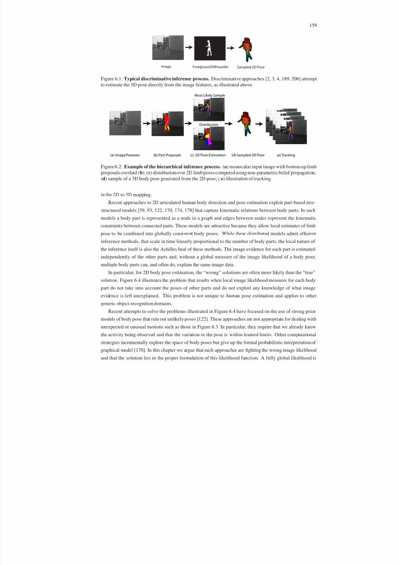
8/13/2019 Continuous-State Graphical Models for Object Localization, Pose Estimation and Tracking
http://slidepdf.com/reader/full/continuous-state-graphical-models-for-object-localization-pose-estimation 174/220
159
Image Sampled 3D PoseForeground Silhouette
Figure 6.1: Typical discriminative inference process. Discriminative approaches [2, 3, 4, 189, 206] attempt
to estimate the 3D pose directly from the image features, as illustrated above.
(a) Image/Features (b) Part Proposals (c) 2D Pose Estimation (e) Tracking(d) Sampled 3D Pose
Distribution
Most Likely Sample
Figure 6.2: Example of the hierarchical inference process. (a) monocular input image with bottom up limb
proposals overlaid (b); (c) distribution over 2D limb poses computed using non-parametric belief propagation;
(d) sample of a 3D body pose generated from the 2D pose; ( e) illustration of tracking.
in the 2D to 3D mapping.
Recent approaches to 2D articulated human body detection and pose estimation exploit part-based tree-
structured models [59, 93, 122, 170, 174, 178] that capture kinematic relations between body parts. In such
models a body part is represented as a node in a graph and edges between nodes represent the kinematic
constraints between connected parts. These models are attractive because they allow local estimates of limb
pose to be combined into globally consistent body poses. While these distributed models admit efficient
inference methods, that scale in time linearly proportional to the number of body parts, the local nature of
the inference itself is also the Achilles heal of these methods. The image evidence for each part is estimated
independently of the other parts and, without a global measure of the image likelihood of a body pose,
multiple body parts can, and often do, explain the same image data.
In particular, for 2D body pose estimation, the “wrong” solutions are often more likely than the “true”
solution. Figure 6.4 illustrates the problem that results when local image likelihood measures for each body
part do not take into account the poses of other parts and do not exploit any knowledge of what image
evidence is left unexplained. This problem is not unique to human pose estimation and applies to other
generic object-recognition domains.Recent attempts to solve the problems illustrated in Figure 6.4 have focused on the use of strong prior
models of body pose that rule out unlikely poses [122]. These approaches are not appropriate for dealing with
unexpected or unusual motions such as those in Figure 6.3. In particular, they require that we already know
the activity being observed and that the variation in the pose is within learned limits. Other computational
strategies incrementally explore the space of body poses but give up the formal probabilistic interpretation of
graphical model [170]. In this chapter we argue that such approaches are fighting the wrong image likelihood
and that the solution lies in the proper formulation of this likelihood function. A fully global likelihood is

8/13/2019 Continuous-State Graphical Models for Object Localization, Pose Estimation and Tracking
http://slidepdf.com/reader/full/continuous-state-graphical-models-for-object-localization-pose-estimation 175/220
160
Figure 6.3: Silly walks. The detection of 2D body pose in real images is challenging due to complex back-
ground appearance, loose monochromatic clothing, and the sometimes unexpected nature of human motion.In this scene, strong, activity-dependent, prior models of human pose are too restrictive. The result here was
found by our method which makes weak assumptions about body pose but uses a new occlusion-sensitive
image likelihood.
computationallyimpractical and consequently we develop a principled approximation to the global likelihood
that is sensitive to local occlusion relationships between parts.
The resulting 2D pose estimation is an adaptation of the loose-limbed body model introduced in the previ-
ous chapter for the purposes of monocular 2D pose estimation. As before, simple body part detectors provide
noisy probabilistic proposals for the location and 2D pose (orientation and foreshortening) of visible limbs
(Figure 6.2 (b)). The pose is estimated by inference in the view-based 2D graphical model representation of
the body. As before we also use a variant of non-parametric belief propagation (PAMPAS) [99, 220] to infer
probability distributions representing the belief in the 2D pose of each limb (Figure 6.2 (c)). The inference
algorithm also introduces hidden binary occlusion variables and marginalizes over them to account for occlu-
sion relationships between body parts. The bi-directional conditional distributions linking 2D body parts are
learned from examples (similarly to Chapter 5).
This process of using limb proposals and non-parametric inference in a graphical model provides reason-
able guesses for 2D body pose from which to estimate the 3D pose of the body. Sminchisescu et al. [206]
and Agarwal and Triggs [2] learned a probabilistic mapping from 2D silhouettes to 3D pose using a Mixture
of Experts (MoE) model. We extend their approach to learn a mapping from 2D poses (including joint angles
and foreshortening information) to 3D poses. The approach uses a mixture of regularized linear regression
models that are trained from a set of 2D-3D pose pairs obtained from motion capture data.
Sampling from this model provides predicted 3D poses (Figure 6.2 (d)), that are appropriate as proposals
for a Bayesian temporal inference process (Figure 6.2 (e)). Our multi-stage approach overcomes many of
the problems inherent in inferring 3D pose directly from image features. The proposed hierarchical Bayesian
inference process copes with the complexity of the problem through the use of intermediate generative 2D
model.

8/13/2019 Continuous-State Graphical Models for Object Localization, Pose Estimation and Tracking
http://slidepdf.com/reader/full/continuous-state-graphical-models-for-object-localization-pose-estimation 176/220
161
(a) (b) (c)
0 5 10 15 20 25 30 35 40 45 50−2.165
−2.16
−2.155
−2.15
−2.145
−2.14x 10
6
L o g
L i k e l i h o o d
Frame #
Occlusion−sensitive true poseOcclusion−sensitive alternative pose (b)Occlusion−sensitive alternative pose (c)Pictorial structures true posePictorial structures alternative pose (b)Pictorial structures alternative pose (c)
Figure 6.4: Fighting the likelihood. (a) shows the ground truth body pose while (b) and (c) show common
failure modes of pictorial structure approaches in which both legs explain the same image data. With local
image likelihoods, the poses in (b) and (c) are often better interpretations of the scene than the true pose.
This can be seen in the plot where 50 frames of a test sequence are evaluated. The blue curves illustrate the
local pictorial structures likelihood. The likelihood of the ground truth is solid blue while the likelihoods forthe two alternative poses (both legs front or both legs back) are shown as dashed lines. The local likelihood
marginally prefers the true pose in only 2 out of 50 frames tested. With our proposed occlusion-sensitive
likelihood (shown in red) the true pose is always more likely than the alternative poses.
We qualitatively and quantitatively evaluate our 2D pose estimation procedure, comparing the perfor-
mance to the state-of-the-art discrete tree-structured model of Felzenszwalb and Huttenlocher [59] and results
published in [122]. We show that our continuous-state, occlusion-sensitive, model is better suited, in terms
of quantitative performance, for 2D pose inference. We also quantitatively evaluate the 3D proposals using
ground truth 2D poses. Finally, we test the full hierarchical inference strategy proposed in this chapter on the
monocular sequence in Figure 6.2. We test both automated 3D pose inference from monocular static frames,
as well as tracking.
6.1 Previous Work
Generative, model-based, approaches for recovering 2D articulated pose can be loosely classified into two
categories. Top-to-bottom approaches treat the body as a “cardboard person” [111] in which the limbs are
represented by 2D patches connected by joints. These patches are connected in a kinematic tree [30, 52, 90,

8/13/2019 Continuous-State Graphical Models for Object Localization, Pose Estimation and Tracking
http://slidepdf.com/reader/full/continuous-state-graphical-models-for-object-localization-pose-estimation 177/220
162
147, 173, 193, 209] and the pose of the person is represented by a high-dimensional state vector that includes
the position and orientation of the root limb in the global image coordinate frame and the parameters of each
limb relative to its parent in the tree. The high-dimensional state space makes exhaustive search for the body
pose difficult. While impractical for pose estimation from a single frame, these methods have been shown to
be appropriate and effective for tracking.
In contrast, bottom-up approaches address the dimensionality of the state space by representing each part
independently in the 2D image coordinate frame. In such models a body part is represented as a node in
a graph and edges in the graph represent kinematic constraints between connected parts. This formulation
allows independent search for the parts which are then combined subject to the kinematic constraints. The
results are typically imprecise, but enable automatic initialization (pose estimation). These “Pictorial Struc-
tures” approaches assume the graph of the body is a tree, which makes inference tractable [59, 170, 178].
While efficient Belief Propagation inference methods1 in these graphical models exist [59], they require a
discretization of the state space of 2D limb poses and simple forms for the conditional distributions relating
connected limbs (see discussion in Section 3.5.2).
The pictorial structures approach also has problems as illustrated in Figure 6.4 where multiple body parts
explain the same image regions. The problems arise from the assumption that the global image likelihood
can be expressed as a product of individual local terms (one per part), without regard to occlusions. As a
result, as shown in Figure 6.4, we find that the true pose is almost always (in 48 out of 50 frames tested)
less likely than the alternative hypothesis that corresponds to the local maximum. To deal with this, previous
algorithms have sampled multiple poses from the solution space and then used an external global likelihood
to choose among the sampled hypothesis [59]. This approach however requires smoothing of likelihood
functions, to ensure that the true pose is sampled. The direct maximum a posteriori2 (MAP) estimate of
the posterior almost always results in the undesired solution. Alternatively, Ramanan and Forsyth [170] first
find a solution for one side of the body and then remove the image regions explained by that solution from
future consideration. They then solve for the other side of the body independently. While this sidesteps the
problem it does not explicitly model the possible occlusion relationships and the algorithmic solution looses
the probabilistic elegance present in the graphical model formulation. A more recent approach of Kumar
et al. [121] acknowledges that occlusions of parts must be accounted for and proposes a layered pictorial
structure model that exhaustively searches over the depth-based layering of parts. The resulting approach is
more robust, but requires video for on-line learning of the layering model.
Alternatively one can impose strong global constraints on the allowed poses that prohibit solutions like
those in Figure 6.4 (b) and (c) [122]. In [122] a single latent variable that accounts for the unmodeled
correlation between parts of the body is added. This may be appropriate when the activity is known and the
range of poses is highly constrained; for example, walking poses can be represented using a small number
of hidden variables [160]. We argue that these strong priors are invoked to deal with inadequate imagelikelihoods. In Figure 6.4 the local likelihoods prefer the wrong solutions and hence the prior is fighting with
the likelihood to undo its mistakes. Furthermore strong priors are unable to cope with unusual activities such
1 Belief Propagation inference in these graphical models can be recast and solved using dynamic programming.
2 Maximum a posteriori (MAP) (a.k.a. posterior mode) estimation is often used to obtain a point estimate of the posteriordistribution.
It is closely related to maximum likelihood (ML) estimation, but can incorporate a prior distribution over the variables, and hence can be
seen as a regularization of ML estimation. Often the MAP estimate is computed in the cases where the expected value of the posterior
density cannot be computed explicitly.

8/13/2019 Continuous-State Graphical Models for Object Localization, Pose Estimation and Tracking
http://slidepdf.com/reader/full/continuous-state-graphical-models-for-object-localization-pose-estimation 178/220
163
as the one in Figure 6.3.
The closest work to ours, addresses the problem with the image likelihoodsin these decentralized models
in the context of 3D articulated hand pose estimation [219]. They explicitly model occlusions in 3D and
deal with distributed reasoning in graphical models using Non-parametric Belief Propagation [220]. The
approach deals with the issue of overcounting image evidence but does not address the problem of having the
model explain as much of the image evidence as possible locally. As a result the particular message passing
order must be imposed to account for the layering of parts. They also only deal with tracking from a hand
initialized pose; here we go further to deal with automatic pose estimation (initialization). Consequently,
our formulation allows for more general likelihoods. Our framework also uses a slightly different inference
approach, from the one introduced in [220], that extends the basic Particle Message Passing (PAMPAS)
algorithm introduced in previous chapters.
In summary, to address articulated 2D pose estimation from monocular static imagery, we propose a
method for approximating the global likelihood using consistent local likelihoods. This allows us to use a
part-based graphical model of the body and perform inference with a generic approximate BP algorithm,
PAMPAS. Unlike [59] we deal with the continuous estimation of part locations, orientation, foreshortening
and scale. Like previous approaches, for now we assume a known view but multiple views can be searched
simultaneously and it is relatively straightforward to compare the results to select the best view. Without
strong priors, the method finds solutions that better explain the image evidence, and results in more accurate
pose estimation. Also, unlike previous methods [59, 196] we infer 2D pose as an intermediate step to inferring
the full 3D articulated body pose.
Lee and Cohen [127] also use a bottom-up proposal process and infer 3D pose parameters using a data-
driven MCMC procedure. Our approach differs in that we break the problem into simpler pieces: generate
2D proposals, inference of 2D pose, and prediction from 2D to 3D. We are also able to incorporate temporal
coherence (tracking) where appropriate.
The 2D to 3D inference stage has received a good deal of attention with a variety of geometric [147,
222] and machine learning methods [2, 3, 4, 181, 189, 206] being employed. Most previous approaches
have focused on directly inferring 3D pose from 2D silhouettes which may be difficult to obtain in general.
Additionally silhouettes contain less information than our 2D models which represent all the limbs, the joint
angles, and foreshortening. This helps reduce the ambiguities found in matching silhouettes to 3D models
[209] but does not remove ambiguities altogether. Consequently we learn a conditional distribution using
a Mixture of Experts (MoE) model similar to that of Sminchisescu [206] and Agarwal and Triggs [2]. Our
work is similar in spirit to [90] in which 3D poses are inferred from 2D tracking results, but our approach can
infer 3D pose from a single monocular image and does not require manual initialization.
6.2 Modeling a Person
We model a 3D human body using a set of P (here P = 10) tapered cylinders corresponding to body parts
and connected by revolute joints. Each part has an associated set of fixed parameters that are assumed to be
known (e.g. length and cross-sectional radius at the two joints). We represent the overall pose of the body
Yt = [Ξt, Γt, Θt]T at time t using a set of joint angles Θt, a global position Ξt, and global orientation Γt
in 3D. Joint angles are represented with respect to the kinematic chain along which they are defined using

8/13/2019 Continuous-State Graphical Models for Object Localization, Pose Estimation and Tracking
http://slidepdf.com/reader/full/continuous-state-graphical-models-for-object-localization-pose-estimation 179/220

8/13/2019 Continuous-State Graphical Models for Object Localization, Pose Estimation and Tracking
http://slidepdf.com/reader/full/continuous-state-graphical-models-for-object-localization-pose-estimation 180/220
165
7
6
1
2 4
3 5
8
9
10
X1
X10 X2 X4 X6 X8
X3 X5 X7 X9
ψK ij
(b)
X1
X10 X2 X4 X6 X8
X3 X5 X7 X9
ψK ij
ψOij(c)
X2
X4
V 2, V 2
V 4, V 4
I
I
X1
X3
X1
X5
(a) (d)
Figure 6.5: Representing 2D body as a graph. Figure (a) shows the representation of the 2D body as agraph with bodyparts labeled using the corresponding node numbers; (b) shows the corresponding tree-based
representation of the body, and (c) our extended body model that contains additional occlusion constraints
designated by edges in blue; (d) shows actual directed graphical model interactions encoded by a single blue
edge in (c) between X2 and X4; I is the image evidence.
Global vs. Local Image Likelihoods
Given the state of the body X, we define a global likelihood φ(I |X) in terms of some features I (with slight
abuse of notation) observed in an image. For continence, we assume that these features are defined per-
pixel and on a pixel grid. To support distributed modeling of the body we write this global likelihood as the
product of local likelihood terms φ(I
|X)
∝ i∈
[1,...,P ] φi(I
|Xi). Drawing inspiration from [59] and [260],
we define local likelihoods, as in previous chapter, in terms of the product of individual pixel likelihoods
in sub-regions of the image that are defined by the local state Xi. For clarity we re-state the likelihood
formulation introduced in Section 5.4, in a slightly more general form, here.
Formally, we assume that pixels in an feature image, I , can be partitioned into three disjoint sub-sets
Ω1(Xi) ∪ Ω2(Xi) ∪ Ω3(Xi) = Υ, where Υ is the set of all pixel grid positions u ≡ (x, y) in an image;
Ω1(Xi) is the set of pixels enclosed by part i as define by the state Xi; Ω2(Xi) contains the pixels outside
part i that are statistically correlated with the part i (for example pixels in the border slightly outside the

8/13/2019 Continuous-State Graphical Models for Object Localization, Pose Estimation and Tracking
http://slidepdf.com/reader/full/continuous-state-graphical-models-for-object-localization-pose-estimation 181/220
166
limb); and Ω3(Xi) ≡ Υ − (Ω1(Xi) ∪ Ω2(Xi)) which corresponds to the set of pixels where we assume no
correlation of the image statistics based on the pose of part i. Assuming pixel independence in the feature
image, we write the local likelihood φ(I |Xi) for the part i as a product of individual pixel probabilities as
φi(I
|Xi) = u∈Ω1(Xi)
p1(I u) s∈Ω2(Xi)
p2(I s) r∈Ω3(Xi)
p3(I r) (6.1)
for features I u, u = (x, y) ∈ Υ.
The standard pictorial structures silhouette likelihood, (denoted by F G in Chapter 5) [59] can easily be
written in this form,
φi,fg(I |Xi) =
u∈Ω1(Xi)
p1,FG(I u)
s∈Ω2(Xi)
p2,FG(I s)
r∈Ω3(Xi)
p3,FG(I r), (6.2)
by letting I u be a silhouette image obtained by background subtraction ( i.e. I u ≡ F Gc(x, y) using notation
of Chapter 5) and by setting
p1,FG(I u) =
q 1 if I u = 1
1 − q 1 otherwise
p2,FG(I u) =
q 2 if I u = 1
1 − q 2 otherwise
p3,FG(I u) = 0.5 (6.3)
for some constants 0 ≤ q i ≤ 1. For other non binary features such as limb/skin color (denoted here by C ) we
can express p1,C (I u) and p2,C (I u) as a per pixel ratio of learned foreground and background distributions;
for example
p1,C (I u) = pskin(I u)
pskin(I u) + pbkgd(I u)
p2,C (I u) = pbkgd(I u)
pskin(I u) + pbkgd(I u)
p3,C (I u) = 0.5 (6.4)
where I u, in this case, is simply a pixel value of the original image.
Occlusion-sensitive Local Likelihoods
The above formulation is only valid if the local terms φi(I |Xi) for i ∈ [1,...,P ] are independent. In absence
of occlusions, this assumption holds and likelihoods factor. When limbs occlude each other, however, the
assumption does not hold and the product of local likelihoods gives a poor approximation to the global
likelihood (see Figure 6.4).
To allow a similar decomposition (and hence distributed inference) when occlusions exist, we augment
the state, Xi, of limb i with two sets of binary hidden variables V i = vi,u and V i = vi,u, where u is
a pixel u ∈ Υ. Let vi,u = 0 if pixel u for the part i is occluded by any other body part, and 1 otherwise.

8/13/2019 Continuous-State Graphical Models for Object Localization, Pose Estimation and Tracking
http://slidepdf.com/reader/full/continuous-state-graphical-models-for-object-localization-pose-estimation 182/220
167
Intuitively this corresponds to the “visibility” of the part i at a given pixel u. Notice that if vi,u = 1 for some
pixel u ∈ Ω1(Xi), then we know that part i at a given pose Xi generated pixel u in the image. Similarly we
let vi,u = 0 if at pixel u for part i at Xi is occluding any other part, and 1 otherwise. Intuitively V i encodes
which pixels in the image could possibly be explained by other body parts that are further away from the
camera. In particular, if vi,s = 1 and vi,s = 1 for a pixel slightly outside part i, s
∈ Ω2(Xi), then that pixel,
s, must have been generated by a background model (since by definition there cannot be any other part in
front or behind i at s). Intuitively V i and V i in conjunction allow the likelihood to not only be sensitive to
occlusions [219] but also to reason locally about globally plausible explanations of the image. In other words,
each limb maintains a summary of what is in front and behind it via binary masks V i and V i.
An illustration of these visibility variables is shown in Figure 6.6. For example, Figure 6.6 (c) indicates
that the torso is occluded by the lower arm ( vi,u = 0) and Figure 6.6 (g) indicates that the arm is occluding
part of the torso (vi,u = 0).
Modifying our likelihood, to take into account the hidden per-pixel binary occlusion variables we have
φi(I |Xi, V i, V i) = u∈Ω1(Xi)
[ p1(I u)]vi,u s∈Ω2(Xi)
[ p2(I s)]vi,svi,s r∈Ω3 (Xi)
[ p3(I r)]vi,rvi,r . (6.5)
Notice that vi,u and vi,u are simply used as selectors. If pixel u ∈ Ω1(Xi) is unoccluded then contribution of
pixel u, p1(I u), to the likelihood will be considered. Similarly, if pixel s ∈ Ω2(X1) is both unoccluded and
unexplained then its contribution will be considered as well. Pixels for which vi,u = 0 and/or vi,u = 0 will
have constant likelihood 1.
The per-pixel occlusion-sensitive likelihoods are shown in Figure 6.6 for the torso ( e) and lower arm
(h). The local estimate of the global likelihood is simply the product of the pixel likelihoods, where brighter
indicates more likely.
It is important to note that conditioned on the sets of hidden variables V i and ˆV i the local likelihoods
φi(I |Xi, V i, V i) are truly independent if V i and V i are consistent across all i ∈ [1,...,P ]. By consistency
here we mean that parts do not assume mutually occluding states for example (meaning that there may exist
only one part i for which vi,u = 1, for all others vj,u = 0, where j ∈ [1,...,P ]/i). This ensures that
φ(I |Y) ∝ i∈[1,...,P ] φi(I |Xi, V i, V i) always holds.
6.3.2 Modeling Constraints
The 2D body in our decentralized model is represented by constraints between the parts that express tradi-
tional kinematic relationships (similar to those described in Section 5.3.1 but in 2D) as well as occlusion
relationships between possibly occluding parts.
Occlusion Constraints
Enforcing the consistency of the hidden occlusion variables V i and V i requires reasoning that involves all
potentially occluding and occluded parts for any given node i. We can express these occlusion constraints
using pairwise potential functions ψOij(Xj, V j, V j ,Xi, V i, V i) between every pair of potentially occluding
parts i and j . We formally encode the consistency of all occlusion relationships between part i and j using
the unnormalized distribution:

8/13/2019 Continuous-State Graphical Models for Object Localization, Pose Estimation and Tracking
http://slidepdf.com/reader/full/continuous-state-graphical-models-for-object-localization-pose-estimation 183/220
168
(a) (c) (d) (e)
(b) (f ) (g) (h)
Figure 6.6: Occlusion-sensitive likelihood. Two overlapping parts (torso and lower arm) are shown in ( a).
The solid regions correspond to Ω1 while the regions outside but enclosed by the line correspond to Ω2. (b)
shows the observed silhouette; (c) and (f ) show the state of the hidden variables V i for the torso and left
lower arm respectively; (d) and (g) show the corresponding states of the V i’s; (e) and (h) shows the per pixel
local occlusion-sensitive likelihoods with pixel brightness corresponding to high probability. Notice that inthe cases where a part is both occluded and occluding other parts, both V i and V i will contain non-uniform
structure.
ψOij(Xj, V j , V j ,Xi, V i, V i) ∝u∈Υ
0 if Xj occludes Xi, u ∈ Ω1(Xj), vi,u = 1
0 if Xi occludes Xj, u ∈ Ω1(Xi), vj,u = 1
0 if Xj occludes Xi, u ∈ Ω1(Xi), vj,u = 1
0 if Xi occludes Xj, u ∈ Ω1(Xj), vi,u = 1
1 otherwise
(6.6)
Intuitively this simply enumerates all inconsistent cases and assigns them 0 probability. The first case for
example can be interpreted as the following: if Xj occludes Xi and any pixel u is inside the image region of
occluding part j , then vi,u corresponding to the visibility of the occluded part i at the pixel u must be set to
0.
Kinematic Constraints
Every pair of connected parts (i, j) in the body also has an associated kinematic potential function that
enforces kinematic constraints and positions of joints. As before, see Section 5.3.1, potentials are modeled

8/13/2019 Continuous-State Graphical Models for Object Localization, Pose Estimation and Tracking
http://slidepdf.com/reader/full/continuous-state-graphical-models-for-object-localization-pose-estimation 184/220
169
using convienient robust Gaussian mixture representation but in 2D. Also, as before, we learn the conditional
distributions, corresponding to these potential functions, directly instead of indirectly deriving them from the
joint distributions (see discussion in Section 5.3.1). The conditional distributions were learned separately for 8
view-based models using 3D motion capture data. The trainingmotion capture data was partitioned according
to the relative heading of the body with respect to the camera viewing direction at 45 degree increments. The
3D body pose was projected into a desired camera view and the conditionals were learned from the 2D
projections of individual limbs. As before, we used a standard iterative Expectation-Maximization (EM)
algorithm with K-means initialization for learning the Gaussian mixture model (GMM) (see Algorithm 1 in
Section 3.4.2 for details). For all experiments in this chapter we used M ij = 8 mixture components.
6.3.3 Inference
Inference in the standard pictorial structures model involves estimating the location and pose of every body
part. With our occlusion-sensitive model we have the additional problem of dealing with the hidden occlusion
variables. Given the formulation above, the joint probability for the graphical model with P body parts, can
be written as
p(X1,X2,...,XP |I ) ∝V i
V i
[ij
ψK ij (Xj ,Xi) (6.7)
ij
ψOij(Xj , V j, V j,Xi, V i, V i)j
φi(I |Xj , V j, V j)]
where Xi represents the state of the limb i; ψK ij (Xj ,Xi) is the kinematic compatibility term between the
connected nodes i and j ; ψOij(Xj, V j, V j ,Xi, V i, V i) is the occlusion compatibility between potentially oc-
cluding nodes i and j and φi(I
|Xi, V i, V i) is the local image likelihood. The two summations marginalize
over the hidden occlusion variables in V i and V i. Notice, unlike other graphical models introduced in this the-
sis where the states are either continuous or discrete, the model introduced here has both continuous variables
(corresponding to the 2D location of parts) and discrete variables (corresponding to per-pixel occlusions).
We solve for the part poses using belief propagation where the message update equations are:
mK ij (Xj) =
Xi
V i
V i
[ψK ij (Xj ,Xi)
φi(I |Xi, V i, V i)
k∈A/jmK ki(Xi)mO
ki(Xi, V i, V i)], (6.8)
mOij(Xj, V j, V j) =
Xi
V i
V i
[ψOij(Xj , V j, V j ,Xi, V i, V i)
φi(I |Xi, V i, V i)
k∈A/jmK ki(Xi)mO
ki(Xi, V i, V i)]. (6.9)
Inferring the state of the 2D body in our graphical model representation corresponds to estimating the
belief (marginal) at each node in a graph,

8/13/2019 Continuous-State Graphical Models for Object Localization, Pose Estimation and Tracking
http://slidepdf.com/reader/full/continuous-state-graphical-models-for-object-localization-pose-estimation 185/220
170
(a) (b)
(c)
Figure 6.7: Occlusion-sensitive inference. Figure (a) shows the proposal distributions for the six body parts
drawn from the ground truth pose and corrupted by Gaussian noise. Both left and right calves are initialized
intentionally incorrectly on the left calf in the image; (b) shows the mean of the marginal distribution for each
part after 3 iterations of belief propagation (BP). Figure(c) shows 100 samples from the marginal distributions
after one, two and three iterations of BP. Notice that we initialize from a local maximum of the traditional
likelihood function, precisely the place where most algorithms get “stuck”, yet our algorithm is still able to
recover the correct pose.
bi(Xi) =V i
V i
φi(I |Xi, V i, V i)k∈A
mK ki(Xi)mO
ki(Xi, V i, V i). (6.10)
We use PAMPAS [99], as in previous chapters, to deal with this task. The messages are approximated
using a kernel density formed by propagating particles through a conditional density (see Section 3.7 for
details). In all the experiments we used 100 particles which, when propagated through the conditionals
represented by mixtures of 8 Gaussians, resulted in density representation for the messages with N = 800
Gaussian kernels. We modify the method to include an annealing step [52] with each iteration of P AMPAS,
as discussed in Section 3.7.7, that gradually introduces the effects of peaks in our local likelihoods. For the
details on how the message updates are carried out using stratified sampling from the products of messages
and a static proposal distribution see Algorithm 6 in Section 3.7. The illustration of the inference using
PAMPAS with occlusion-sensitive likelihoods can be seen in Figure 6.7. Consequently, in Figure 6.7 we
start intentionally from undesired initial conditions, where both legs are found in the same location; yet our
occlusion-sensitive model is able to successfully recover from this local maximum.

8/13/2019 Continuous-State Graphical Models for Object Localization, Pose Estimation and Tracking
http://slidepdf.com/reader/full/continuous-state-graphical-models-for-object-localization-pose-estimation 186/220

8/13/2019 Continuous-State Graphical Models for Object Localization, Pose Estimation and Tracking
http://slidepdf.com/reader/full/continuous-state-graphical-models-for-object-localization-pose-estimation 187/220
172
Limb Proposals
Plausible poses/states for some or all the body parts are needed as proposals to initiate inference (see Sec-
tion3.7.3). There exist a number of efficient methods for detecting2D bodyparts in an image [127, 147, 176].
Among them approaches for face detection [236], skin color-based limb segmentation [127, 128], and color-
based segmentation exploiting the homogeneity and the relative spatial extent of body parts [127, 128, 147,176]. Here we took a simple approach and constructed a set of proposals by coarsely discretizing the state
space and evaluating local part-based likelihood functions at these discrete locations. For all of the exper-
iments here we discretized the state space into 5 scales, 5 foreshortenings, 20 vertical and 20 horizontal
positions, and 8 rotations. Out of 5 × 5 × 20 × 20 × 8 = 80, 000 evaluated discrete states, we chose the 100
most likely states for each part and used these as a particle based proposal distribution for belief propagation.
It is important to note that not all parts need to be detected and, in fact, detecting all the parts is largely
impossible due to the self occlusions. To initialize the search we used, as in Chapter 5, proposals for 6 parts:
torso, head and four outermost extremities. All other parts were initialized with a uniform distribution over
the entire state space.
6.4 Proposing 3D Body Model from 2D
In order to produce estimates for the body in 3D from the 2D body poses, we need to model the conditional
distribution p(Y|X) of the 3D body state Y given 2D body state X. Intuitively this conditional mapping
should be related to the inverse of the camera projection matrix and, as with many inverse problems, is highly
ambiguous.
To model this non-linear relationship we use a Mixtures of Experts (MoE) model to represent the con-
ditionals [3, 4, 206]. The more complete definition of MoE model and the learning procedure can be found
in Section 3.8.2, here we briefly restate3 the process for convenience. The parameters of the MoE model are
learned by maximizing the log-likelihood of the training data set D = (x1, y1),..., (xN , yN ) consisting of
N input-output pairs (xi, yi). We use an iterative Bayesian EM algorithm, based on maximum likelihood, to
learn parameters of the MoE. Our model for the conditional can be written as:
p(Y|X) =M m=1
pe(Y|X, zm = 1, θe,m) pg(zm = 1|X, θg,m) (6.13)
where pe(Y|X, zm = 1, θe,m) is the probability of choosing poseY given the inputX according to the m-th
expert, and pg(zm = 1|X, θg,m) is the probability of that input being assigned to the m-th expert using an
input sensitive gating network; in both cases θ represents the parameters of the mixture and gate distributions.
For simplicity and to reduce complexity of the experts we choose linear regression with constant offset
Y = β X + α as our expert model (this is a simple generalization of the linear regression model described
in Section 3.8.1), which allows us to solve for the parameters θe,m = β m, αm, Σm analytically using the
weighted linear regression. The expert model can be written as follows:
3 Notice that hereX is thevariable we are conditioningon andY is the variable we are trying to infer; opposite is true forthe notation
in Section 3.8.2.

8/13/2019 Continuous-State Graphical Models for Object Localization, Pose Estimation and Tracking
http://slidepdf.com/reader/full/continuous-state-graphical-models-for-object-localization-pose-estimation 188/220
173
X1
X10 X2 X4 X6 X8
X3 X5 X7 X9
ψK ij
ψOijX
Y
time
Y1 Y2 Y3 YT
I 1 I 2 I 3 I T
ψT
(a) (b) (c)
Figure 6.8: Hierarchical inference. Graphical model representation of the hierarchical inference process;
(a) illustrates the 2D body model used for inference of the 2D pose at every frame, with kinematic constraints
marked in black, and occlusion constraints in blue, and (c) the Hidden Markov Model (HMM) used for
inferring and tracking the state of the 3D body, Yt, over time t ∈ [1,...,T ], using the hierarchical inference
proposed, in which proposals for each node, Y , are constructed from 2D body pose X using the model in
(b).
pe(Y|X, zm = 1, θe,m) = 1 (2π)dY |Σm| exp−
12 ∆T
mΣ−1m ∆m , (6.14)
where dY is the dimensionality of the 3D pose Y, β m and αm regression parameters, Σm is the covariance
of the kernel regressor, and
∆m = Y − β mX− αm. (6.15)
Pose estimation is a high dimensional and ill-conditioned problem, so simple least squares estimation
of the linear regression matrix parameters typically produces severe over-fitting and poor generalization.
To reduce this, we add smoothness constraints on the learned mapping. We use a damped regularization
term R(β ) = λ||β ||2 that penalizes large values in the coefficient matrix β , where λ is a regularization
parameter (a.k.a. ridge regression). Larger values of λ will result in overdamping, where the solution will be
underestimated, small values of λ will result in overfitting and possibly ill-conditioning. Since the solution of
the ridge regressors is not symmetric under the scaling of the inputs, we normalize the inputs x1, x2,...,xN by the standard deviation in each dimension respectively before solving 4 .
The weighted ridge regression solution for the parameters β k and αk can be written in matrix notation as
follows,
β m
αm T
= DT X
diag(Z m) DX + diag(λ) Z m
Z T m Z T mZ m −1
DT X
Z T m diag(Z m)
DY, (6.16)
where Z m = [z(1)m , z(2)
m ,...,z(N )m ]T is the vector of ownership weights described later in the section and
diag(Z m) is diagonal matrix with Z m on the diagonal; DX = [x1, x2,...,xN ] and DY = [y1, y2,...,yN ] are
4To avoid problems with 2D and 3D angles that wrap around at 2π, we actually regress the (cos(θ), sin(θ)) representation for 2D
angles and unit quaternion q = [qx, qy , qz , qw]T representation for 3D angles. After the 3D pose is reconstructed we normalize the
not-necessarily normalized quaternions to valid 3D rotations. Since quaternions also suffer from the double cover problem, where two
unit quaternions correspond to every rotation, care must be taken to ensure that consistent parameterization is used.

8/13/2019 Continuous-State Graphical Models for Object Localization, Pose Estimation and Tracking
http://slidepdf.com/reader/full/continuous-state-graphical-models-for-object-localization-pose-estimation 189/220
174
vectors of inputs and outputs formed from the training data D.
Maximization for the gate parameters can be done analytically as well. Given the gate model,
pg(zm = 1|X, θg,m) = 1
(2π)dX |Λm| exp−
12 (X−µm)T Λ−1
m (X−µm) (6.17)
maximization of the gate parameters θg,m = (Λm, µm) becomes similar to the mixture of Gaussians estima-
tion, where
µm =
N n=1
z(n)m xn/
N n=1
z(n)m (6.18)
Λm = 1N n=1 z
(n)m
N n=1
z(n)m [xn − µm][xn− µm]T (6.19)
and z(n)m is the estimated ownership weight of the example n by the expert m estimated by expectation
z(n)m = pe(yn|xn, z
(n)
m = 1, θe,m) pg(z
(n)
m = 1|xn, θg,m)M j=1 pe(yn|xn, z(n)
j = 1, θe,j) pg(z(n)j = 1|xn, θg,j)
. (6.20)
The above outlines the full EM procedure for the MoE model. We learn MoE models for two classes of
actions: walking and dancing. Examples of the ground truth 2D query poses with corresponding expected 3D
body poses can be seen in Figure 6.9 (a) and (b) respectively. Similar to [3, 4] we initialize the EM learning
by clustering the output 3D poses using the K-means procedure. We learn a single conditional MoE model
that we use for all view-based 2D pose estimates. We experimented with learning of view-based conditional
MoE models, but they tended to have artifacts at view boundaries and suffered from overfitting.
Implementation Details
Instead of learning the full conditional model p(Y|X), we learn two independent models p(Γ|X) and p(Θ|X)
one for the pose of the 3D body p(Θ|X) given the 2D body pose X, and one for the global orientation of the
body p(Γ|X). The reasoning for this is twofold. First, this partitions the learned mapping into a fully camera-
independent model for the pose p(Θ|X), and the more specific camera-dependent model for the orientation of
thebody in theworld p(Γ|X). Second, we found that the optimal damping coefficient is significantly different
for the two models, therefore imposing a single joint conditionalmodel (and hence a single coefficient) would
result in somewhat larger reconstruction error. Estimation of the depth p(Ξ|X) is done analytically (using
simple regression) by considering the estimated position and overall scale of the 2D body.
6.5 Tracking in 3D
Once the distribution for the 3D body pose at every frame is inferred using the conditional MoE model
described, we can incorporate temporal constraints to regularize the individual 3D pose estimates by track-
ing. We exploit the relatively standard undirected variant of the Hidden Markov Model (HMM) shown in
Figure 6.8 (c). To infer the state of Yt at every frame t given the temporal potential ψT (Yt,Yt+1) =
N (Yt −Yt+1; 0, ΣT ), with learned covariance matrix ΣT , we use the same inference framework of PAM-
PAS. Unlike many competing approaches, we allow the model to optimize the pose estimates not only forward

8/13/2019 Continuous-State Graphical Models for Object Localization, Pose Estimation and Tracking
http://slidepdf.com/reader/full/continuous-state-graphical-models-for-object-localization-pose-estimation 190/220
175
W a l k i n
g
D a n c i n g
(a) (b) (c) (d) (e)
Figure 6.9: Proposed 3D pose. (a) Synthetic query 2D body pose, obtained from projected motion capture
data; (b) expected 3D pose produced by the learned action-specific Mixture of Experts (MoE) model. (c)
Ground-truth 3D body pose; (d) and (e) illustrate the projection of the expected 3D pose shown in (b) onto
the original and one alternative image view.
but also backward in time in a batch (this amounts to temporal smoothing).
The likelihood, φ(I t|Yt), of observing the 3D pose Yt at time t given image evidence I t is defined
in terms of Chamfer distance of the projected pose Yt to the silhouettes and edges obtained from I t using
standard techniques.
6.6 Experiments
In this section we present a set of quantitative and qualitative experimental results for testing various stages
of our hierarchical inference framework, as well as the framework as a whole. We first test how well we can
recover the 2D pose independently in each frame using our occlusion-sensitive loose-limbed body model in
Section 6.6.1; we then analyze how well our discriminative MoE model can predict the 3D pose from the 2D
poses recovered at every frame, in Section 6.6.2; finally, we briefly explore the benefits of adding temporal

8/13/2019 Continuous-State Graphical Models for Object Localization, Pose Estimation and Tracking
http://slidepdf.com/reader/full/continuous-state-graphical-models-for-object-localization-pose-estimation 191/220
176
0 5 10 15 20 25 30 35 40 45 505
10
15
20
25
30
35
40
45
Frame #
P o s e E s t i m a t i o n E r
r o r ( p i x )
PAMPAS−OS
PAMPAS−Tree
PS−Tree
Figure 6.10: Quantitative performance evaluation of 2D pose estimation. Mean error of the joint locationsfor each frame of 50 frame image sequence with ground truth [197]. For the description of the metric see
text.
consistency (tracking) into our hierarchical framework in Section 6.6.3.
6.6.1 Monocular 2D Pose Estimation
We learned occlusion-sensitive models for 8 discrete views of a person including frontal, side and 3/4 views.
For each view we assume the depth ordering of the body parts is known. The kinematic constraints between
parts were learned from projected motion capture data. In all experiments the likelihood uses a combination
of silhouette and color/intensity information (assuming independence). Color was primarily used to achieve
robustness in the cases where silhouettes were ambiguous or unreliable in localizing a given part. For the
silhouette likelihood we used the pictorial structures type model and learned p1,FG(I u = 1 ) = q 1 and
p2,FG (I s = 1) = q 2 using the procedure described in [59]. Similar to [59] we assumed that p3,FG(I r = 1) =
0.5. For the color/intensity likelihood we learned a kernel density model for each part and the background.
For frontal views, the lack of self occlusion means that tree based approaches will usually perform well.
Consequently we focus on the more challenging side-views containing occlusion. We quantitatively compare
our approach (PAMPAS-OS) to leading tree-based methods using 50 frames from the Brown ground truth
sequence, obtained similarly to the H UMANEVA-I dataset described in Section 5.7.1. Unlike HUMANEVA-
I, the dataset used in this chapter contains images from 4 synchronized greyscale cameras (instead of 7
in HUMANEVA-I); however, we only employ images from one camera (BW1) for inference. Additional
description of the data used in this chapter will be given in the next section. To evaluate performance of our
2D method, we extend the error metric presented in Chapter 5. As before, the proposed metric computes
the average distance error between a set of 15 virtual marker locations corresponding to the joints. However,
since our pose in this case is in 2D, the distance is computed in the image plane, instead of the world; the
resulting error is in ( pixels).
For comparison we implemented two tree-based methods: pictorial structures (PS-Tree) [59] and a variant

8/13/2019 Continuous-State Graphical Models for Object Localization, Pose Estimation and Tracking
http://slidepdf.com/reader/full/continuous-state-graphical-models-for-object-localization-pose-estimation 192/220
177
Strong Discrete Mean Error Std. of Error
Prior State ( pixels) ( pixels)
PAMPAS-OS No No 10.33 2.25
PAMPAS-Tree No No 16.40 3.67
PS-Tree No Yes 20.84 6.64
PS-Tree [122] No Yes 13.79 3.99
LBP [122] Yes Yes 12.00 3.99Factor [122] Yes Yes 6.42 1.55
Figure 6.11: Overall performance comparison of 2D pose estimation. Performance of the occlusion-
sensitive inference compared with two tree-based algorithms implemented by us. We also compare to the
results reported by [122] on the same image sequence.
of our approach that does not model occlusions (PAMPAS-Tree) by simply removing the occlusion constraints
from our model. Figure 6.10 shows the mean error for 15 markers at every frame for the three methods; the
statistics, for comparison, are shown in Figure 6.11. Following [122] we deal with the left/right ambiguity by
switching the left/right limbs and reporting the interpretation with a smallest error. Notice, that for the results
reported in Figures 6.10 and 6.11 we are estimating the pose independently at every frame (i.e. only doing
pose estimation, not tracking).
Our occlusion-sensitive inference approach outperforms pictorial structures by 50% (25% for the im-
plementation in [122]1). We found that occlusion-reasoning accounts for a 37% performance gain over the
simple PAMPAS-Tree method. According to the published literature [122] our approach also outperforms
max-product loopy-BP, but does not do as well as the common-factor model (Factor) presented in [122]. This
is not surprising, since the common-factor model uses a walking prior learned for this data. Our approach
does not assume a strong prior on the motion or style, instead it only encodes weak prior 5 on the relative
position of neighboring limbs.
Figure 6.12 illustrates the behavior of PS-Tree, PAMPAS-Tree and PAMPAS-OS on a few frames of the
sequence. As expected we observed many failures in the pictorial structures model due to the overlapping
parts (e.g. see Figure 6.12 (a)). PAMPAS-Tree, not surprisingly had similar modes of failure while the
occlusion-sensitive PAMPAS-OS does a better job of explaining the image evidence (as can be seen from
the results in Figure 6.11 and quantitative comparison in Figure 6.10).
In addition to the quantitative experiments we also ran our model on less structured scenarios from TV
and movies for which strong prior models will typically not work. Figure 6.13 illustrates two representative
results. In both cases, camera motion makes background subtraction difficult. Crude background subtraction
was obtained using homographies estimated between 2 frames sufficiently far apart in time (using the code
from http://www.robots.ox.ac.uk/∼vgg/). Estimated homographies allow us to compensate for the
camera motion and use frame differencing to obtain very rough estimates for the foreground silhouette (see
Figure 6.13 (c)). Color likelihoods were defined as in [170].
Our current un-optimized implementation of PAMPAS-OS in Matlab takes roughly 5 minutes for mes-
sage passing, and 1.5 minutes for belief estimation per frame. The occlusion constraints account for a 43%
1 Our independent implementation of PS-Tree [59] resulted in somewhat larger error than reported in [122].
5 Consequently, while in this thesis we advocate the use of weak prior models due to their generality, the models introduced here do
not prevent the use of strong priors. To the contrary, the loose-limbed models we introduced can easily be extended to include priors of
the form explored in [122] to boost performance in specific domains.

8/13/2019 Continuous-State Graphical Models for Object Localization, Pose Estimation and Tracking
http://slidepdf.com/reader/full/continuous-state-graphical-models-for-object-localization-pose-estimation 193/220
178
(a)
(b)
(c)
Frame 2 Frame 24 Frame 49
Figure 6.12: Visual performance evaluation of 2D pose estimation. (a) MAP estimates for the tree-based
implementation of pictorial structures on three frames from our test sequence. Performance of occlusion-
insensitive and occlusion-sensitive PAMPAS is shown in (b) and (c) respectively. The top rows show 100samples from the marginal distribution at every node (belief) after 5 iterations of BP, and bottom rows the
weighted mean computed over those samples. BP was run using 100 particles which resulted in the N = 800Gaussian kernel mixtures for the messages.
overhead over PAMPAS-Tree.
6.6.2 Monocular 3D Pose Estimation
In previous section we tested the performance of one of the key components of our hierarchical framework,
that allows us to reliably recover the 2D pose of the person from monocular images (independently at every
frame). We showed that our occlusion-sensitive model performs better then other methods tested. In this

8/13/2019 Continuous-State Graphical Models for Object Localization, Pose Estimation and Tracking
http://slidepdf.com/reader/full/continuous-state-graphical-models-for-object-localization-pose-estimation 194/220
179
(a)
(b)
Figure 6.13: Occlusion-sensitive reasoning in movies. Results on frames from TV/films. Left column in (a)
and (b) shows 100 samples from the marginal distribution (belief) after 3 iterations of BP, and right column
shows the weighed mean pose. In both cases very rough and noisy background subtraction was obtained by
estimating homographies between 2 frames from the sequence sufficiently far apart in time. Example of the
rough background subtraction obtained in this way for the image in (b) is illustrated in the last row.
section, we investigate the second major component of our framework, that allows us to infer the 3D pose of
the person from 2D pose estimates; for now, still from single monocular images. We first conduct a set of
synthetic experiments that allows us to quantitative test how well our Mixture of Experts (MoE) model can
recover 3D pose in general, assuming the 2D pose is known 6. We than show how this learned MoE model
can be used to recover the 3D pose from the real 2D poses obtained in the previous section.
Datasets. For all experiments presented in this section we used two datasets that exhibit two different
types of actions: walking and dancing. Both datasets contain a number of motion capture examples used
for training, and a single synchronized motion capture example with multi-view video used for testing (the
same as in previous section). Video was captured using 4 stationary grayscale cameras at 60 Hz, and 3D
pose was captured using a Vicon system at 120 Hz. The motion capture (mocap) was aligned to video
and sub-sampled to 60 Hz, to produce synchronous video/mocap streams. All cameras were calibrated using
standard calibration procedures. Walking dataset [197] contains 4587 training and 1398 testing poses/frames;
dancing: 4151 training and 2074 testing poses/frames.
6 We use projected motion capture data in lieu of known 2D poses.

8/13/2019 Continuous-State Graphical Models for Object Localization, Pose Estimation and Tracking
http://slidepdf.com/reader/full/continuous-state-graphical-models-for-object-localization-pose-estimation 195/220

8/13/2019 Continuous-State Graphical Models for Object Localization, Pose Estimation and Tracking
http://slidepdf.com/reader/full/continuous-state-graphical-models-for-object-localization-pose-estimation 196/220
181
Figure 6.9) and the error for the reconstructed 3D poses7 was analyzed (see Figure 6.15).
We consider 3 variants of the base error metric: (Pose) 3D body pose error computed by first aligning the
global coordinate frames of the reconstructed and ground truth body, (View) global body orientation error
computed by first aligning the reconstructed pose/articulation with the ground truth pose/articulation, and
(View+Pose) an overall error for the reconstructed state Y. The alignment for (View) and (Pose) is done by
simply using the ground truth portion of the 3D pose for the corresponding components of the state vector.
The key observation is that walking, being considerably simpler of the two action types, can be recovered
significantly better (with 50% less error), than the more complex dancing. The peaks in the error in both
cases often correspond to singular or close to singular instances where foreshortening in the pose of 2D limbs
for example is severe; similar singularities arise where the pose of the entire body is close to lateral or frontal
(with unbent arms and legs), where the view itself is singular (i.e. the model can’t easily distinguish between
left and right, or front and back, orientation of the body when singularities occur).
Real Experiments. We can also apply the learned walking Mixture of Experts (MoE) model to the
real 2D poses obtained in Section 6.6.1. This allows us to recover the full 3D pose automatically, using
the proposed hierarchical method, from single monocular image; results are illustrated in Figure 6.16. The
3D poses look very reasonable, however, the right arm that is occluded in 2D in most frames is often miss
estimated. Notice, that the prior over walking postures, implicitly embedded into the action-specific walking
MoE model, allows the conditional model to correct some of the errors made by the 2D pose estimation
component.
6.6.3 Monocular 3D Tracking
In Sections 6.6.1 and 6.6.2 we experimented with two major components of our hierarchical inference method
that, in conjunction, allow the inference of 3D pose from monocular single images. In this section, we briefly
illustrate how these individual 3D pose estimation results can be regularized by Bayesian temporal inference
(Figure 6.17).
Our experiments with hierarchical single-frame method, illustrated in Section 6.6.2, show that while the
method can reasonably recover the 3D pose, it cannot reliably resolve the left/right ambiguity of the body.
In other words, the inference method often switches the identity of the two legs from frame to frame (see
frames 17–19 in Figure 6.18); in general, it is ambiguous to reason about left/right leg identity from the
lateral view images illustrated in Figure 6.16. In addition, the recovered poses are also often noisy (jittery).
We found temporal smoothing, results of which are illustrated in Figure 6.17, to be useful in regularizing this
intra-frame variability in pose. Consequently, temporal smoothing produces more coherent tracks over time
as illustrated in Figure 6.18.
6.7 Conclusion and Discussion
The automatic estimation of human pose and motion from monocular image data remains a challenging
problem. Here we have proposed a framework to address this problem that uses hierarchal Bayesian inference
to go from crude body part detections to a distribution over 3D body pose. We make modest assumptions
about the availability of noisy body part detectors and a reasonable image likelihood model.
7 Supplementary videos are available from http://www.cs.brown.edu/people/ls/ .

8/13/2019 Continuous-State Graphical Models for Object Localization, Pose Estimation and Tracking
http://slidepdf.com/reader/full/continuous-state-graphical-models-for-object-localization-pose-estimation 197/220
182
200 400 600 800 1000 1200 1400 1600 1800 20000
50
100
150
200
250
300
350
400
Frame
E r r o r ( m m )
View Only [mean = 22.046905 (mm)]Pose Only [mean = 59.037876 (mm)]View + Pose [mean = 64.040940 (mm)]
1 2 3 4 5 6 7 8 9 10 11 12 13 140
50
100
150
200
250
300
350
H i p L e f t
K n e e L e f t
A
n k l e L e f t
H i p
R i g h t
K n e e
R i g h t A n
k l e
R i g h t
S h o u l d e r L e f t
E l b o w L e f t
W r i s t L e f t
S h o u l d e r R i g h t
E l b o w
R i g h t W
r i s t R i g h t
N e c k
H e a d
Joint
E r r o r ( m m )
ViewPose
(a) (b)
200 400 600 800 1000 12000
50
100
150
200
250
300
350
400
Frame
E r r o r ( m m )
View Only [mean = 14.470740 (mm)]Pose Only [mean = 23.085540 (mm)]View + Pose [mean = 29.502635 (mm)]
1 2 3 4 5 6 7 8 9 10 11 12 13 140
50
100
150
200
250
300
350
H i p L e f t K
n e e L e f t
A n k l e L e f t
H i p
R i g h t
K n e e
R i g h t
A n k l e
R i g h t
S h o u l d e r L e f t
E l b o w L e f t
W r i s t L e f t
S h o u l d e r R i g h t
E l b o w
R i g h t
W r i s t R i g h t
N e c k
H e a d
Joint
E r r o r ( m m )
ViewPose
(c) (d)
Figure 6.15: Quantitative evaluation of action-specific conditional model. The model, p(Y|X) = p(Ξ
|X) p(Γ
|X) p(Θ
|X), is tested by comparing the expectation to ground truth data for two classes of motion.
Per-frame error for the reconstructed 3D pose Θ, global orientation Γ, and the full 3D state of the body Y are
shown for dancing in (a) and walking in (c); the average per-joint error as compared to the ground truth is
shown in (b) and (d) respectively.
We use belief propagation to infer 2D limb poses that are consistent with the human body model. Note
that we make no strong assumptions about the prior poses of the body. Our approach extends recent work
on inferring 3D body models from 2D silhouettes by using the inferred 2D articulated model instead. This
provides a richer representation which reduces ambiguities in the 2D to 3D mapping. We also show that the
3D pose proposals can be used in a tracking framework, that can further regularize the 3D pose estimates.
As part of this hierarchical inference strategy, we also introduce a novel approach for articulated 2D body
pose estimation that uses occlusion-sensitive local image likelihoods that approximate the global likelihood
by accounting for occlusions and competing explanations of image evidence by multiple parts. We model
occlusion relationships between parts explicitly by introducing two sets of per-pixel hidden binary variables
for each part. Intuitively these variables model which pixels are explained by which parts when multiple
parts project to the same image regions. The resulting occlusion reasoning involves interactions between
non-adjacent parts which introduces loops in the graphical model representation of the body. To achieve
tractable real-valued inference in such a graph, we also introduced an extension to the approximate belief

8/13/2019 Continuous-State Graphical Models for Object Localization, Pose Estimation and Tracking
http://slidepdf.com/reader/full/continuous-state-graphical-models-for-object-localization-pose-estimation 198/220
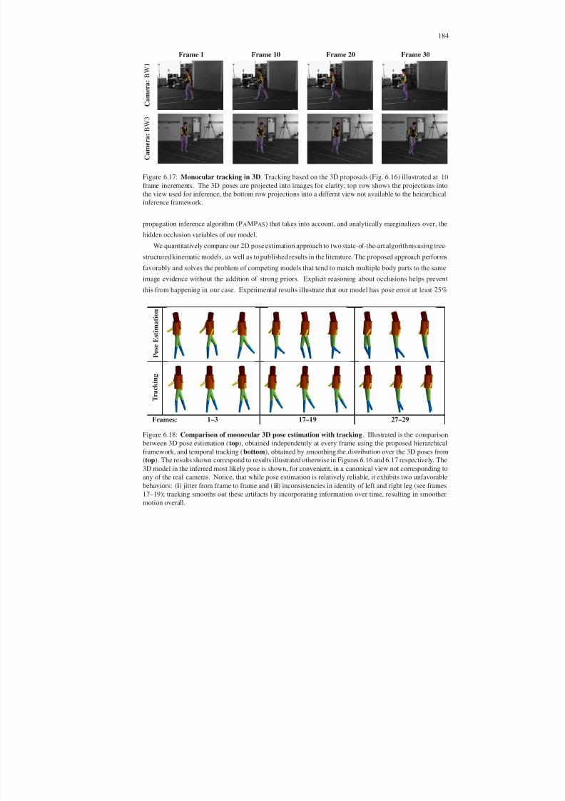
8/13/2019 Continuous-State Graphical Models for Object Localization, Pose Estimation and Tracking
http://slidepdf.com/reader/full/continuous-state-graphical-models-for-object-localization-pose-estimation 199/220
184
Frame 1 Frame 10 Frame 20 Frame 30
C a m e r a : B W 1
C a m e r a : B W 3
Figure 6.17: Monocular tracking in 3D. Tracking based on the 3D proposals (Fig. 6.16) illustrated at 10frame increments. The 3D poses are projected into images for clarity; top row shows the projections into
the view used for inference, the bottom row projections into a differnt view not available to the heirarchical
inference framework.
propagation inference algorithm (PAMPAS) that takes into account, and analytically marginalizes over, the
hidden occlusion variables of our model.
We quantitatively compare our 2D pose estimation approach to two state-of-the-art algorithms using tree-
structured kinematic models, as well as to published results in the literature. The proposed approach performs
favorably and solves the problem of competing models that tend to match multiple body parts to the same
image evidence without the addition of strong priors. Explicit reasoning about occlusions helps prevent
this from happening in our case. Experimental results illustrate that our model has pose error at least 25%
P o s e E s t i m a t i o n
T r a c k i n g
Frames: 1–3 17–19 27–29
Figure 6.18: Comparison of monocular 3D pose estimation with tracking. Illustrated is the comparisonbetween 3D pose estimation (top), obtained independently at every frame using the proposed hierarchical
framework, and temporal tracking (bottom), obtained by smoothing the distribution over the 3D poses from
(top). The results shown correspond to results illustrated otherwise in Figures 6.16 and 6.17 respectively. The
3D model in the inferred most likely pose is shown, for convenient, in a canonical view not corresponding to
any of the real cameras. Notice, that while pose estimation is relatively reliable, it exhibits two unfavorable
behaviors: (i) jitter from frame to frame and (ii) inconsistencies in identity of left and right leg (see frames
17–19); tracking smooths out these artifacts by incorporating information over time, resulting in smoother
motion overall.

8/13/2019 Continuous-State Graphical Models for Object Localization, Pose Estimation and Tracking
http://slidepdf.com/reader/full/continuous-state-graphical-models-for-object-localization-pose-estimation 200/220

8/13/2019 Continuous-State Graphical Models for Object Localization, Pose Estimation and Tracking
http://slidepdf.com/reader/full/continuous-state-graphical-models-for-object-localization-pose-estimation 201/220
CHAPTER 7
Summary and Discussion
In this thesis we introduced a novel class of models and corresponding inference algorithms that are able to
address a variety of common problems in object localization, pose estimation and tracking. For the large
portion of this thesis we concentrated on the challenging class of articulated objects (i.e. people). Dealing
with people is challenging, particularly because of variation in appearance and articulations; furthermore, the
pose of the person often requires representations that are high-dimensional and that must deal with ambiguous
image observations. Reasoning about people and their pose in images, is popular however, due to the vast
number applications in animation, surveillance, biomechanics and human computer interaction.
Instead of attempting to battle the dimensionality of the state-space and complexity of motion directly, we
formulate the problem of pose estimation and tracking as one of inference in a graphical model. The nodes in
this graph correspond to parts of the body and edges to kinematic, inter-penetration and occlusion constraints
imposed by the structure of the body and the imaging process. This model, which we call a loose-limbed
body model, allows us to infer the 3D pose of the body effectively and tractably from multiple synchronized
views; or a 2D pose of the body from a single monocular image, in time linear in the number of articulatedparts. Unlike previous decentralized models, we work directly with continuous variables, and use variants of
Particle Message Passing (PAMPAS) for inference.
In addition, we also introduced hierarchical models for both articulated and generic object reasoning. In
the case of generic objects, hierarchy facilitates tractable inference by ensuring that the temporal constraints
are only propagated on the object level and not at the level of individual parts. In the case of articulated
objects, hierarchy also mediates the complexity of the spatial inference, by allowing the model to first infer
the 2D pose of the body in the image plane, then infer the 3D pose from the 2D body pose estimates and
lastly apply the temporal continuity (tracking) at the 3D pose level. This leads to two important benefits: (1)
the hierarchical model helps to reduce the depth and projection ambiguities by looking at a full 2D body pose
rather then the pose of individual limbs, and (2) it gives a modular, tractable, and fully probabilistic solutionthat allows inference of 3D pose from a single monocular image in an unsupervised fashion.
In all cases we have shown both qualitatively and qualitatively that the models introduced perform as
well, or better, then other state-of-the-art methods.
186

8/13/2019 Continuous-State Graphical Models for Object Localization, Pose Estimation and Tracking
http://slidepdf.com/reader/full/continuous-state-graphical-models-for-object-localization-pose-estimation 202/220
187
7.1 Future Work
While the models we introduced are effective and address a number of common problems in both articulated
and rigid object motion estimation, there still a number of issues that must be addressed in the future to make
these models widely applicable for large categories of objects.
7.1.1 Faster Inference Algorithms
Particle Message Passing (PAMPAS) and various extensions thereof, that have been introduced in this thesis,
while tractable and have linear complexity, still are too slow to allow real-time (30 frames per second) pro-
cessing on current hardware. The main computational bottleneck, is that sampling from products of messages,
represented by kernel densities with many mixture components, is computationally expensive. Reducing the
number of mixture components in the representation of messages would lead to significant computational
speedup of PAMPAS. On an intuitive level, while the kernel densities that we are using to approximate
messages are complex, the underlying distributions that they are approximating are often, in comparison,
relatively simple (particularly after BP has converged or is close to convergence).
To speed up inference there have been recent attempts to develop faster Non-parametric Belief Propa-
gation (NBP) inference algorithms by automatically reducing representation of the message to a number of
prominent modes estimated by Mean-shift [78]. The results have been shown to be orders of magnitude faster
then simple NBP or PAMPAS, for tracking. Our preliminary experiments (not described in this thesis), have
shown that this approach indeed achieves significant speedups for simple examples where messages are close
to convergence (i.e. have few modes). For pose estimation, where the messages are often initialized relatively
far from the true solution, the process of reducing the number of mixture components in the representation,
takes longer then the inference itself. A simple explanation for this is that the number of modes in a message
in this case is typically significantly larger (tens instead of one or two that are often observed in tracking).
We believe that hybrid algorithms that reduce message representation complexity only when possible, is thenext logical step in producing tractable inference algorithms for this class of models.
Other approaches that we believe may be useful in reducing the complexity of inference are hybrid
Markov Chain Monte Carlo methods, that can be used to replace the pure Monte Carlo sampling engine
of PAMPAS. Hybrid methods have been shown to achieve faster (orders of magnitude faster) inference in
other domains [38], and we believe can be relatively easily adopted for the use in the PAMPAS framework.
7.1.2 Deeper Hierarchical Models
We found hierarchical models to be very effective in managing both computational and modeling complexity
of problems addressed by this thesis. Currently, however, we restricted ourselves to models with relatively
few (2 to 3) levels. In such models each level in the hierarchy has a pre-defined semantic structure. Deep
hierarchical networks (a.k.a. deep belief networks) [82, 83] have been successfully developed and applied
in other applications. In these deep networks, however, layers typically lack semantic interpretation as the
number of layers grows and the layers themselves are learned automatically using unsupervised methods. We
believe that, in the context of object modeling, particularly of articulated object modeling, slightly deeper
hierarchies (than the ones presented in this thesis) can be developed that can both be useful and still maintain
the semantic interpretation. For example, currently the interactions of different views and features are all

8/13/2019 Continuous-State Graphical Models for Object Localization, Pose Estimation and Tracking
http://slidepdf.com/reader/full/continuous-state-graphical-models-for-object-localization-pose-estimation 203/220
188
rolled into the likelihood function in our framework. Using additional layers in the hierarchical model, these
interactions can be made explicit and perhaps better modeled. Our current likelihood model, for example,
assumes independence across features and across views. A more explicit model can potentially model cor-
relations between these variables. In particular, as the number of views increase, the observations become
less and less independent. This is not currently handled by the models introduced in this thesis (nor much of
related literature).
7.1.3 Learning of Model Structure
In this thesis we showed that continuous-state graphical models are effective means of modeling objects and
drawing inferences about these objects, particularly pertaining to position and configuration of these objects
in space. The models that we presented were built using the expert domain knowledge of the object class,
that involved knowing and leveraging kinematic structure of the object with complexity of inference. The
parameters of those models were learned in semi-supervised fashion, from motion capture data in the case of
humans or hand annotated images in the case of vehicles. These models provide a very productive paradigm
for object reasoning, due to the linear complexity that stems from their decentralized nature.The problem of building these models automatically from unlabeled (or weakly labeled) data, however,
is still largely unaddressed. In the context of Machine Learning, this problem is often referred to as graphical
model structure learning. While it has been addressed in the context of some specific classes of graphical
models, for example, in parametric Bayesian networks that have no interactions between hidden variables
[200, 201], the case of general undirected graphical models with non-parametric continuous random variables
is still largely unexplored. Continuous non-parametric models are considerably more expressive which makes
model structure learning hard. To our knowledge, the only approach that addresses structure learning in
general graphs that have both continuous and discrete variables was introduced by Bach and Jordan [12]. The
ability to build these rich models automatically, however, is the key to making them widely applicable in the
domain of generic object recognition.
In the context of articulated human motion, the ability to build models automatically would allow building
of action-specific models that could potentiallymodel higher order action-specific correlations between limbs.
For example, in walking, there are well known correlations between upper and lower extremities and left and
right sides of the body. Other motions may exhibit similar correlation patterns, induced by subtle hidden
causes like gravity, balance, and/or intent. Building models that can automatically find, and account for, such
correlations would undoubtedly lead to better models and performance.
7.1.4 Scene Parsing
One of the key advantages of using graphical models for modeling objects, beyond tractable inference, isthe ability to combine different models in the context of probabilistic inference. We believe that one of the
prominent directions of future research is to combine models of various objects (or multiple instances of the
same model) for scene parsing and interpretation. Much like in the speech recognition community, context
provided by other objects can be useful in constraining the object(s) of interest (e.g. [85]).

8/13/2019 Continuous-State Graphical Models for Object Localization, Pose Estimation and Tracking
http://slidepdf.com/reader/full/continuous-state-graphical-models-for-object-localization-pose-estimation 204/220
189
7.2 Conclusions
In this thesis we presented a novel class of methods that model people using rich decentralized probabilistic
models. These models have a number of appealing advantages over the centralized models typically em-
ployed. The inference methods, that make use of the decentralized model structure for tractable inference,
have also been introduced. In addition, we introduced a number of extensions to our basic loose-limbed bodymodel, that allowed monocular inference and illustrated inference over simple generic objects (e.g. vehicles).
The next challenge is take the methods introduced in this thesis and extend them for use with generic and
possibly interacting objects. Among the challenges one would have to address, the most predominant are
the unsupervised or semi-supervised learning of the model structure and faster (close to real-time) inference
methods.

8/13/2019 Continuous-State Graphical Models for Object Localization, Pose Estimation and Tracking
http://slidepdf.com/reader/full/continuous-state-graphical-models-for-object-localization-pose-estimation 205/220
BIBLIOGRAPHY
[1] A. Agarwal and B. Triggs. Recovering 3D Human Pose from Monocular Images, IEEE Transactions on Pattern
Analysis and Machine Intelligence (PAMI), Vol. 28, No. 1, pp. 44–58, January 2006.
[2] A. Agarwal and B. Triggs. Monocular Human Motion Capture with a Mixture of Regressors, IEEE Workshop on
Vision for Human-Computer Interaction, pp. 72–79, 2005.
[3] A. Agarwal and B. Triggs. Learning to Track 3D Human Motion from Silhouettes. International Conference on
Machine Learning (ICML), pp. 9–16, 2004.
[4] A. Agarwal and B. Triggs. 3D human pose from silhouettes by relevance vector regression. IEEE Computer Society
Conference on Computer Vision and Pattern Recognition (CVPR), Vol. 2, pp. 882–888, 2004.
[5] S. Agarwal, A. Awan and D. Roth. Learningto detect objects in images via a sparse, part-based representation, IEEE
Transactions on Pattern Analysis and Machine Intelligence (PAMI), Vol. 26, No. 11, pp. 1475–1490, November
2004.
[6] B. Allen, B. Curless, Z. Popovic and A. Hertzmann. Learning a correlated model of identity and pose-dependent
body shape variation for real-time synthesis, Symposium on Computer Animation (SCA), pp. 147–156, 2006.
[7] J. Amores, N. Sebe and P. Radeva. Fast Spatial Pattern Discovery Integrating Boosting with Constellations of
Contextual Descriptors, IEEE Computer Society Conference on Computer Vision and Pattern Recognition (CVPR),
Vol. 2, pp. 769–774, 2005.
[8] D. Anguelov, P. Srinivasan, D. Koller, S. Thrun, J. Rodgers and J. Davis. SCAPE: Shape Completion and Animation
of People, International Conference on Computer Graphics and Interactive Techniques (SIGGRAPH), 24(3):408–
416, 2005.
[9] M. S. Arulampalam, S. Maskell, N. Gordon and T. Clapp. A tutorial on particle filters for online nonlinear/non-
Gaussian Bayesian tracking, IEEE Transactions on Signal Processing, Vol. 50, Issue 2, pp. 174–188, February
2002.
[10] V. Athitsos, J. Wang, S. Sclaroff and M. Betke. Detecting Instances of Shape Classes That Exhibit Variable Struc-
ture, European Conference on Computer Vision (ECCV), Vol. 1, pp. 121–134, May 2006.
[11] V. Athitsos, J. Alon, S. Sclaroff and G. Kollios. BoostMap: A Method for Efficient Approximate Similarity Rank-
ings, IEEE Computer Society Conferenceon Computer Vision and Pattern Recognition (CVPR), pp. 268–275, June
2004.
[12] F. R. Bach and M. I. Jordan. Learning graphical models with Mercer kernels, Advances in Neural Information
Processing Systems (NIPS), Vol. 15, 2003.
190

8/13/2019 Continuous-State Graphical Models for Object Localization, Pose Estimation and Tracking
http://slidepdf.com/reader/full/continuous-state-graphical-models-for-object-localization-pose-estimation 206/220
191
[13] A. Balan, L. Sigal, M. J. Black, J. Davis and H. Haussecker. Detailed Human Shape and Pose from Images, IEEE
Computer Society Conference on Computer Vision and Pattern Recognition (CVPR), 2007.
[14] A. Balan, L. Sigal and M. J. Black. A Quantitative Evaluation of Video-based 3D Person Tracking, IEEE Workshop
on Visual Surveillance and Performance Evaluation of Tracking and Surveillance, pp. 349–356, October 2005.
[15] A. Banerjee, I. S. Dhillon, J. Ghosh and S. Sra. Clustering on the Unit Hypersphere using von Mises-Fisher Distri-
butions, Journal of Machine Learning Research, Vol. 6, pp. 1345–1382, 2005.
[16] H. Bay, T. Tuytelaars and L. van Gool. SURF: Speeded Up Robust Features, European Conference on Computer
Vision (ECCV), Vol. 1, pp. 404–417, 2006.
[17] S. Belongie, J. Malik and J. Puzicha. Matching shapes, International Conference on Computer Vision (ICCV), pp.
454–461,2001.
[18] J. Berclaz, F. Fleuret and P. Fua. Robust People Tracking with Global Trajectory Optimization, IEEE Computer
Society Conference on Computer Vision and Pattern Recognition(CVPR), Vol. 1, pp. 744–750, 2006.
[19] J. Bernardo and A. Smith. Bayesian Theory, John Wiley, New York, 2000.
[20] S. Bhatia, L. Sigal, M. Isard and M. J. Black. 3D Human Limb Detection using Space Carving and Multi-view
Eigen Models, IEEE Workshop on Articulated and Nonrigid Motion, 2004.
[21] J. Bilmes.A Gentle Tutorial on the EM Algorithm andits Application to Parameter Estimation forGaussian Mixture
and Hidden Markov Models, ICSI-TR-97-021, 1997.
[22] C. M. Bishop. Pattern Recognition and Machine Learning, Springer , 2006.
[23] M. J. Black and P. Anandan. A framework for the robust estimation of optical flow. International Conference on
Computer Vision (ICCV), pp. 231–236, 1993.
[24] A. Blake and M. Isard. Active Contours. Springer-Verlag,1998.
[25] A. Blake and M. Isard. The Condensation Algorithm – conditional density propagation and applications to visual
tracking Advances in Neural Information Processing Systems, pp. 361–368, 1997.
[26] X. Boyen and D. Koller. Tractable Inference for Complex Stochastic Processes, Conference on Uncertainty in
Artificial Intelligence (UAI), pp. 33–42, 1998.
[27] E. Boyer. On Using Silhouettes for Camera Calibration, Proceedingsof the seventh Asian Conference on Computer
Vision (ACCV), pp. 1–10, 2006.
[28] E. Boyer and J.-S. Franco. A Hybrid Approach for Computing Visual Hulls of Complex Objects, IEEE Computer
Society Conference on Computer Vision and Pattern Recognition (CVPR), Vol. 1, pp. 695–701, 2003.
[29] M. Brand. Shadow Puppetry, International Conference on Computer Vision (ICCV), Vol. 2, pp. 1237–1244, 1999.
[30] C. Bregler and J. Malik. Tracking people with twists and exponential maps, IEEE Computer Society Conference on
Computer Vision and Pattern Recognition (CVPR), pp. 8–15, 1998.
[31] T. Brox, B. Rosenhahn, U. Kersting and D. Cremers. Nonparametric Density Estimation for Human Pose Tracking,
Symposium of the German Association for Pattern Recognition (DAGM) , Springer-Verlag, LNCS 4174, pp. 546–
555, 2006.

8/13/2019 Continuous-State Graphical Models for Object Localization, Pose Estimation and Tracking
http://slidepdf.com/reader/full/continuous-state-graphical-models-for-object-localization-pose-estimation 207/220
192
[32] W. L. Buntine. Operations for learning with graphical models, Journal of Artificial Intelligence Research, Vol. 2,
pp. 159–225, 1994.
[33] M. Burl, M. Weber and P. Perona. A probabilistic approach to object recognition using local photometry and global
geometry, European Conference on Computer Vision (ECCV), Vol. 2, pp. 628–641, 1998.
[34] T.-J. Cham and J. Rehg. A multiple hypothesisa pproach to figure tracking, IEEE Computer Society Conference on
Computer Vision and Pattern Recognition (CVPR), Vol. 2, pp. 239–245, 1999.
[35] E. Charniak. Statistical Language Learning, MIT Press, Cambridge, Massachusetts, 1993.
[36] G. K. M. Cheung, S. Baker and T. Kanade. Shape-From-Silhouette of Articulated Objects and its Use for Human
Body Kinematics Estimation and Motion Capture, IEEE Computer Society Conference on Computer Vision and
Pattern Recognition (CVPR), Vol. 1, pp. 77–84, 2003.
[37] G. K. M. Cheung, T. Kanade, J. Bouguet and M. Holler. A real time system for robust 3d voxel reconstruction of
human motions, IEEE Computer Society Conference on Computer Vision and Pattern Recognition (CVPR), Vol. 2,
pp. 714–720, 2000.
[38] K. Choo and D. Fleet. People tracking using hybrid Monte Carlo filtering, International Conference on Computer
Vision (ICCV), Vol. 2, pp. 321–328, 2001.
[39] C.-W. Chu, O. C. Jenkins and M. J. Mataric. Markerless Kinematic Model and Motion Capture from Volume
Sequences, IEEE Computer Society Conference on Computer Vision and Pattern Recognition (CVPR), Vol. 2, pp.
475–482, 2003.
[40] P. Clifford. Markov random fields in statistics, Disorder in Physical Systems, pp. 19–32, Oxford University Press,
1990.
[41] D. Comaniciu. An Algorithm for Data-Driven Bandwidth Selection, IEEE Transactions on Pattern Analysis and
Machine Intelligence (PAMI), Vol. 25, No. 2, 281–288, February 2003.
[42] D. Comaniciu and P. Meer. Mean Shift: A Robust Approach toward Feature Space Analysis, IEEE Transactions on
Pattern Analysis and Machine Intelligence (PAMI), Vol. 24, No. 5, pp. 603–619, May 2002.
[43] G. Cooper. The computational complexity of probabilistic inference using Bayesian belif networks, Artificial In-
teligence, Vol. 42, pp. 393–405, 1990.
[44] J. Coughlan and S. Ferreira. Finding deformable shapes using loopy belief propagation, European Conference on
Computer Vision (ECCV), Vol. 3, pp. 453–468, 2002.
[45] G. Csurka, C. Dance, C. Bray, L. Fan and J. Willamowski. Visual categorization with bags of keypoints, In ECCV
workshop on statistical learning in computer vision, 2004.
[46] N. Dalal and B. Triggs. Histograms of Oriented Gradients for Human Detection, IEEE Computer Society Confer-
ence on Computer Vision and Pattern Recognition (CVPR), pp. 886–893, 2005.
[47] R. Dechter. Bucket elimination: A unifying framework for probabilistic inference, Conference on Uncertainty in
Artificial Intelligence, pp. 211–219, 1996.
[48] A. Dempster, N. Laird and D. Rubin. Maximum likelihood from incomplete data via the EM algorithm, Journal of
the Royal Statistical Society, Series B, 39(1):1–38, 1977.
8/13/2019 Continuous-State Graphical Models for Object Localization, Pose Estimation and Tracking
http://slidepdf.com/reader/full/continuous-state-graphical-models-for-object-localization-pose-estimation 208/220
193
[49] J. Deutscher and I. Reid. Articulated body motion capture by stochastic search. International Journal of Computer
Vision (IJCV), Vol. 61, No. 2, pp. 185–205, 2004.
[50] J. Deutscher, M. Isard and J. MacCormick. Automatic camera calibration from a single manhattanimage, European
Conference on Computer Vision (ECCV), Vol. 4, pp. 175–188, 2002.
[51] J. Deutscher, A. Davison and I. Reid. Automatic partitioning of high dimensional search spaces associated with
articulated body motion capture, IEEE Computer Society Conference on Computer Vision and Pattern Recognition
(CVPR), Vol. 2, pp. 669–676, 2001.
[52] J. Deutscher, A. Blake and I. Reid. Articulated body motion capture by annealed particle filtering, IEEE Computer
Society Conference on Computer Vision and Pattern Recognition (CVPR), Vol. 2, pp. 126–133, 2000.
[53] J. Deutscher, B. North, B. Bascle and A. Blake. Tracking through singularities and discontinuities by random
sampling, IEEE International Conference on Computer Vision (ICCV), Vol. 2, pp. 1144–1149, 1999.
[54] A. Doucet, N. de Freitas and N. Gordon. Sequential Monte Carlo methods in practice, Statistics for Engineering
and Infoormation Sciences, Springer Verlag, 2001.
[55] A. Elgammal and C.-S. Lee. Inferring 3D Body Pose from Silhouettes Using Activity Manifold Learning, IEEE
Computer Society Conference on Computer Vision and Pattern Recognition (CVPR), Vol. 2, pp. 681–688, 2004.
[56] G. Elidan, I. McGraw and D. Koller. Residual Belief Propagation: Informed Schedulingfor AsynchronousMessage
Passing, Proceedings of the Twenty-second Conference on Uncertainty in AI (UAI), July 2006.
[57] L. Fei-Fei, R. Fergus and P. Perona. One-Shot learning of object categories, IEEE Transactions on Pattern Analysis
and Machine Intelligence (PAMI), Vol. 28, No. 4, pp. 594–611, April 2006.
[58] L. Fei-Fei and P. Perona. A Bayesian Hierarchical Model for Learning Natural Scene Categories, IEEE Computer
Society Conference on Computer Vision and Pattern Recognition (CVPR), Vol. 2, pp. 524–531, 2005.
[59] P. Felzenszwalb and D. Huttenlocher. Pictorial Structures for Object Recognition, International Journal of Com-
puter Vision (IJCV), Vol. 61, No. 1, pp. 55–79, January 2005.
[60] R. Fergus, P. Perona and A. Zisserman. A Sparse Object Category Model for Efficient Learning and Exhaustive
Recognition, IEEE Computer Society Conferenceon Computer Vision and Pattern Recognition (CVPR), Vol. 1, pp.
380–387, June 2005.
[61] R. Fergus, P. Perona and A. Zisserman. Object Class Recognition by Unsupervised Scale-Invariant Learning, IEEE
Computer Society Conference on Computer Vision and Pattern Recognition (CVPR), Vol. 2, pp. 264–271, 2003.
[62] M. Fischler and R. Elschlager. The representation and matching of pictorial structures, IEEE Transactions on
Computer , 22(1):67–92, January 1973.
[63] J. Foley, A. van Dam, S. Feiner and J. Hughes, Computer Graphics: Principles and Practice, Addison Wesley, ISBN:
0-201-12110-7, 1990.
[64] D. A. Forsyth, O. Arikan, L. Ikemoto, J. O’Brien and D. Ramanan. Computational Studies of Human Motion: Part
1, Tracking and Motion Synthesis, ISBN: 1-933019-30-1, pp. 1–178, July 2006.
[65] J.-S. Franco and E. Boyer. Fusion of Multi-View Silhouette Cues Using a Space Occupancy Grid, IEEE Interna-
tional Conference on Computer Vision (ICCV), Vol. 2, pp. 1747–1753, 2005.

8/13/2019 Continuous-State Graphical Models for Object Localization, Pose Estimation and Tracking
http://slidepdf.com/reader/full/continuous-state-graphical-models-for-object-localization-pose-estimation 209/220
194
[66] Y. Freund and R. E. Schapire. A decision-theoretic generalization of on-line learning and an application to boosting,
Journal of Computer and System Sciences, Vol. 55(1), pp. 119–139, 1997.
[67] Y. Freund and R. E. Schapire. Adecision-theoreticgeneralizationof online learning and an application to boosting,
Unpublished manuscript. An extended abstract appeared in Computational Learning Theory: Second European
Conference (EuroCOLT), Springer-Verlag, pp. 23–37, 1995.
[68] B. J. Frey and N. Jojic. A comparison of algorithms for inference and learning in probabilistic graphical models,
IEEE Transactions on Pattern Analysis and Machine Intelligence (PAMI), Vol. 27, No. 9, pp. 1392–1416, Septem-
ber 2005.
[69] J. Gall, B. Rosenhahn, T. Brox, U. Kersting and H.-P. Seidel. Learning for multi-view 3D tracking in the context
of particle filters, International Symposium on Visual Computing (ISVC), Springer-Verlag, LNCS 4292, pp. 59–69,
2006.
[70] J. Gall, J. Potthoff, C. Schnoerr, B. Rosenhahn and H.-P. Seidel. Interacting and Annealing Particle Filters: Math-
ematics and a Recipe for Applications, Technical Report MPI-I-2006-4-009, Saarbruecken, Germany, September
2006.
[71] F. Grassia. Practical parameterization of rotations using the exponential map, Journal of Graphics Tools, 3(3):29–
48, March 1998.
[72] D. Gavrila and V. Philomin. Real-time Object Detection for Smart Vehicles, IEEE International Conference on
Computer Vision (ICCV), pp. 87–93, 1999.
[73] D. Gavrila. The visual analysis of human movement: A survey, Computer Vision and Image Understanding(CVIU),
73(1):82–98, 1999.
[74] D. Gavrila and L. Davis. 3-D model-based tracking of humans in action: A multi-view approach, IEEE Computer
Society Conference on Computer Vision and Pattern Recognition (CVPR), pp. 73–80, 1996.
[75] S. Geman and D. Geman. Stochastic relaxation, Gibbs distribution and the Bayesian restoration of images, IEEE
Transactions on Pattern Analysis and Machine Intelligence (PAMI), Vol. 6, No. 6, pp. 721–741, 1984.
[76] N. Gordon, D. Salmond and A. Smith. Novel approach to nonlinear/non-Gaussian Bayesian state estimation, IEE
Proceedings F: Radar and Signal Processing, Vol. 140, Issue 2, pp. 107–113, April, 1993.
[77] K. Grauman, G. Shakhnarovich, T. Darrell. Inferring 3D structure with a statistical image-based shape model, IEEE
International Conference on Computer Vision (ICCV), pp. 641–648, 2003.
[78] T. Han, H. Ning and T. Huang. Efficient Nonparametric Belief Propagation with Application to Articulated Body
Tracking, IEEE Computer Society Conference on Computer Vision and Pattern Recognition (CVPR), Vol. 1, pp.
214–221,2006.
[79] C. Harris and M. Stephens. A Combined Corner and Edge Detector, Proceedings of The Fourth Alvey Vision Con-
ference, pp. 147–151, 1988.
[80] W. K. Hastings. Monte Carlo sampling methods using Markov Chains and their applications, Biometrika, Vol. 57,
pp. 97–109, 1970.
[81] D. Haussler, A. Krogh, I. S. Mian and K. Sjolander. Protein modeling using hidden Markov models: Analysis of
globins. Proceedings of the Twenty-Sixth Annual Hawaii International Conference on System Sciences, Vol. 1, pp.
792–802,1993.

8/13/2019 Continuous-State Graphical Models for Object Localization, Pose Estimation and Tracking
http://slidepdf.com/reader/full/continuous-state-graphical-models-for-object-localization-pose-estimation 210/220

8/13/2019 Continuous-State Graphical Models for Object Localization, Pose Estimation and Tracking
http://slidepdf.com/reader/full/continuous-state-graphical-models-for-object-localization-pose-estimation 211/220
196
[100] M. Isard and J. MacCormick. BraMBLe: a Bayesian multiple-blob tracker, IEEE International Conference on
Computer Vision (ICCV), Vol. 2, pp. 34–41, 2001.
[101] T. Izo and E. Grimson. Simultaneous pose recovery and camera registration from multiple views of a walking
person, Image and Vision Computing, 25(3): pp. 342–351, 2007.
[102] T. Izo and E. Grimson. Simultaneous Pose Estimation and Camera Calibration from Multiple Views, Proceedings
of IEEE Workshop on Motion of Non-Rigid and Articulated Objects, Vol. 1, pp. 14–21, June 2004.
[103] R. A. Jacobs, M. I. Jordan, S. Nowlan and G. Hinton. Adaptive mixtures of local experts, Neural Computation,
Vol. 3, pp. 79–87, 1991.
[104] T. Jaeggli, E. Koller-Meier and L. Van Gool. Monocular tracking with a mixture of view-dependentlearned models,
IV Conference on Articulated Motion and Deformable Objects (AMDO), 2006.
[105] F. V. Jensen. Bayesian Networks and Decision Graphs, Springer-Verlag, New York, 2001.
[106] M. Jones and J. Rehg. Statistical Color Models with Application to Skin Detection, International Journal of
Computer Vision (IJCV), Vol. 46, No. 1, pp. 81–96, Jan 2002.
[107] M. I. Jordan. Graphical models, Statistical Science (Special Issue on Bayesian Statistics), Vol. 19, pp. 140–155,
2004.
[108] M. I. Jordan, T. J. Sejnowski and T. Poggio. Graphical models: Foundations of neural computation, MIT Press,
2001.
[109] M. I. Jordan, Z. Ghahramani, T. S. Jaakkola and L. K. Saul. An introduction to variational methods for graphical
models, Machine Learning, Vol. 37, Issue 2, pp. 183–233, 1999.
[110] M. I. Jordan and R. A. Jacobs. Hierarchical mixtures of experts and the EM algorithm. Neural Computation, Vol.
6, pp. 181–214, 1994.
[111] S. Ju, M. J. Black and Y. Yacoob. Cardboard people: A parameterized model of articulated motion, IEEE Interna-
tional Conference on Automatic Face and Gesture Recognition (FG 1996), pp. 38–44, 1996.
[112] I. A. Kakadiaris and D. Metaxas. Model-based estimation of 3D human motion with occlusion based on ac-
tive multi-viewpoint selection, IEEE Computer Society Conference on Computer Vision and Pattern Recognition
(CVPR), pp. 81–87, 1996.
[113] R. Kehl, M. Bray, L. V. Gool. Full Body Tracking from Multiple Views Using Stochastic Sampling. IEEE Com-
puter Society Conference on Computer Vision and Pattern Recognition (CVPR), Vol. 2, pp. 129–136, 2005.
[114] K. Kim and L. Davis. Multi-Camera Tracking and Segmentation of Occluded People on Ground Plane using
Search-Guided Particle Filtering, European Conference on Computer Vision (ECCV), Vol. 3, pp. 98–109, 2006.
[115] K. Kinoshita, Y. Ma, S. Lao and M. Kawade. A fast and robust 3D head pose and gaze estimation system, Interna-
tional Conference on Multimodal Interfaces (ICMI), pp. 137–138, 2006.
[116] S. Kirkpatrick, C. Gellatt and M. Vecchi. Optimisation by simu-lated annealing. Technical report , IBM Thomas J.
Watson Research Centre, Yorktown Heights, NY, USA, 1982.
[117] D. Koller, U. Lerner, and D. Angelov. A general algorithm for approximate inference and its application to hybrid
bayesnets, Proceedings of the 15th Annual Conference on Uncertainty in Artificial Intelligence, pp. 324–333,1999.

8/13/2019 Continuous-State Graphical Models for Object Localization, Pose Estimation and Tracking
http://slidepdf.com/reader/full/continuous-state-graphical-models-for-object-localization-pose-estimation 212/220
197
[118] A. Kong, J. S. Liu and W. H. Wong. Sequential imputations and Baysian missing data problems, Journal of the
American Statistical Association, Vol. 89, pp. 278–288, 1984.
[119] F. R. Kschischang,B. J. Frey, and H.-A. Loeliger. Factor graphs and the sum-product algorithm, IEEE Transactions
on Information Theory, Vol. 47, No. 2, pp. 498–519, Feb 2001.
[120] M. P. Kumar, P. H. S. Torr and A. Zisserman. Learning Layered Motion Segmentation of Video, IEEE Intlerna-tional Conference on Computer Vision (ICCV), pp. 33–40, 2005.
[121] M. P. Kumar, P. H. S. Torr and A. Zisserman. Learning Layered Pictorial Structures from Video, Indian Conference
on Computer Vision, Graphics and Image Processing (ICVGIP), pp. 148–153, 2004.
[122] X. Lan and D. Huttenlocher. Beyond trees: Common factor models for 2D human pose recovery, IEEE Intlerna-
tional Conference on Computer Vision (ICCV), Vol. 1, pp. 470–477, 2005.
[123] X. Lan and D. Huttenlocher. A unified spatio-temporal articulated model for tracking. IEEE Computer Society
Conference on Computer Vision and Pattern Recognition (CVPR), Vol. 1, pp. 722–729, 2004.
[124] Y. LeCun, F. Huang and L. Bottou. Learning Methods for Generic Object Recognition with Invariance to Pose and
Lighting, IEEE Computer Society Conference on Computer Vision and Pattern Recognition (CVPR) , Vol. 2, pp.
97–104, 2004.
[125] C.-S. Lee and A. Elgammal. Simultaneous Inferring View and Body Pose Using Torus Manifolds, International
Conference on Pattern Recognition (ICPR), Vol. 3, pp. 489–494, 2006.
[126] M. Lee and R. Nevatia. Human pose Tracking using multi-level structured models, European Conferenceon Com-
puter Vision (ECCV), Vol. 3, pp. 368–381, 2006.
[127] M. Lee and I. Cohen. Proposal Maps driven MCMC for Estimating Human Body Pose in Static Images, IEEE
Computer Society Conference on Computer Vision and Pattern Recognition (CVPR), Vol. 2, pp. 334–341, 2004.
[128] M. Lee and I. Cohen. Human Upper Body Pose Estimation in Static Images, European Conference on Computer
Vision (ECCV), pp. 126–138, 2004.
[129] S.-I. Lee, V. Ganapathi and D. Koller. Efficient Structure Learning of Markov Networks using L1-Regularization,
Advances in Neural Information Processing Systems (NIPS), 2006.
[130] F. Lerasle, G. Rives and M. Dhome. Tracking of Human Limbs by Multiocular Vision, ComputerVision and Image
Understanding, Vol. 75, Issue 3, pp. 229–246, 1999.
[131] R. Li, M.-H. Yang, S. Sclaroff and T.-P. Tian. Monocular Tracking of 3D Human Motion with a Coordinated
Mixture of Factor Analyzers, European Conference on Computer Vision (ECCV), Vol. 2, pp. 137–150, 2006.
[132] Y. Li, S. Ma and H. Lu. Human Posture Recognition Using Multi-Scale Morphological Method and Kalman
Motion Estimation, International Conference on Pattern Recognition (ICPR), Vol. 1, pp. 175–177, 1998.
[133] Y. Li, A. Hilton and J. Illingworth. A relaxation algorithm for real-time multiview 3d-tracking. Image and Vision
Computing, 20(12):841–59, 2002.
[134] T. Lindeberg. Feature detection with automatic scale selection, International Journal of Computer Vision (IJCV),
Vol. 30, No. 2, pp. 77–116, 1998.
[135] D. G. Lowe. Distinctive image features from scale-invariant keypoints, International Journal of Computer Vision
(IJCV), Vol. 60, No. 2, pp. 91–110, 2004.

8/13/2019 Continuous-State Graphical Models for Object Localization, Pose Estimation and Tracking
http://slidepdf.com/reader/full/continuous-state-graphical-models-for-object-localization-pose-estimation 213/220

8/13/2019 Continuous-State Graphical Models for Object Localization, Pose Estimation and Tracking
http://slidepdf.com/reader/full/continuous-state-graphical-models-for-object-localization-pose-estimation 214/220
199
[153] K. Murphy and S. Russel. Rao-blackwellized particle filtering for dynamic bayesian networks, Sequential Monte
Carlo Methods in Practice, pp. 499–515, Springer, 2001.
[154] C. Musso, N. Oudjane and F. LeGland. Improving regularized particle filters, Sequential Monte Carlo Methods in
Practice, Springer-Verlag, 2001.
[155] R. Neal and G. Hinton. A view of the EM algorithm that justifies incremental, sparse, and other variants. Learningin Graphical Models, pp. 355–368. MIT Press, 1999.
[156] M. Niskanen, E. Boyer and R. Horaud. Articulated Motion Capture from 3-D Points and Normals, British Machine
Vision Conference (BMVC), Vol. 1, pp. 439–448, 2005.
[157] K. Okuma, A. Taleghani, N. De Freitas, J. J. Little and D. Lowe. A Boosted Particle Filter: Multitarget Detection
and Tracking, European Conference on Computer Vision (ECCV), Vol. 1, 28–39, 2004.
[158] A. Opelt, A. Pinz and A. Zisserman. A Boundary-Fragment-Model for Object Detection, EuropeanConference on
Computer Vision (ECCV), Vol. 2, pp. 575–588, 2006.
[159] OpenCV Reference Manual, Intel Open Source Computer Vision Library, available at
http://www.intel.com/research/mrl/research/opencv/.
[160] D. Ormoneit, M. J. Black, T. Hastie, and H. Kjellstrom. Representing cyclic human motion using functional
analysis. Image and Vision Computing, 23(14):1264–1276, Dec. 2005.
[161] C. Papageorgiou and T. Poggio. A Trainable System for Object Detection, International Journal of Computer
Vision (IJCV), Vol. 38, No. 1, pp. 15–33, June 2000.
[162] S. Park and J. K. Aggarwal. A Hierarchical Bayesian Network for Event Recognition of Human Actions and
Interactions, ACM Journal of Multimedia Systems, 10(2), pp. 164–179, 2004.
[163] S. Park and J. K. Aggarwal. Simultaneous Tracking of Multiple Body Parts of Interacting Persons, Computer
Vision and Image Understanding, Vol. 102, Issue 1, pp. 1–21, April 2006.
[164] V. Pavolvic, J. Rehg, T-J. Cham and K. Murphy. A dynamic Bayesian network approach to figure tracking using
learned dynamic models, IEEE International Conference on Computer Vision (ICCV), pp. 94–101, 1999.
[165] R. Plankers and P. Fua. Articulated Soft Objects for Video-based Body Modeling, IEEE International Conference
on Computer Vision (ICCV), pp. 394–401, 2001.
[166] R. W. Poppe and M. Poel. Comparison of Silhouette Shape Descriptors for Example-based Human Pose Recovery,
IEEE International Conference on Automatic Face and Gesture Recognition (FG 2006), pp. 541–546, 2006.
[167] R. Quandt and J. Ramsey. A new approach to estimating switching regressions, Journal of the American Statistical
Society, Vol. 67, pp. 306–310, 1972.
[168] L. R. Rabiner and B. H. Juang. An introduction to hidden Markov models, IEEE ASSP Magazine, pp. 4–15,
January 1986.
[169] D. Ramanan, D. Forsyth and A. Zisserman. Strike a Pose: Tracking People by Finding Stylized Poses, IEEE
Computer Society Conference on Computer Vision and Pattern Recognition (CVPR), Vol. 1, pp. 271–278, 2005.
[170] D. Ramanan, D. Forsyth and K. Barnard. Detecting, Localizing, and Recovering Kinematics of Textured Animals,
IEEE Computer Society Conference on Computer Vision and Pattern Recognition (CVPR), Vol. 2, pp. 635–642,
2005.

8/13/2019 Continuous-State Graphical Models for Object Localization, Pose Estimation and Tracking
http://slidepdf.com/reader/full/continuous-state-graphical-models-for-object-localization-pose-estimation 215/220
200
[171] D. Ramanan and D. Forsyth. Automatic Annotation of Everyday Movements, Neural Information Processing
Systems (NIPS), 2003.
[172] D. Ramananand D. Forsyth. Using temporal coherence to build models of animals, IEEE International Conference
on Computer Vision (ICCV), Vol. 1, pp. 338–346, 2003.
[173] D. Ramanan and D. Forsyth. Finding and tracking people from the bottom up, IEEE Computer Society Conference
on Computer Vision and Pattern Recognition (CVPR), Vol. 2, pp. 467–474, 2003.
[174] X. Ren, A. Berg and J. Malik. Recovering Human Body Configurations using Pairwise Constraints between Parts,
IEEE International Conference on Computer Vision (ICCV), Vol. 1, pp. 824–831, 2005.
[175] C. P. Robert and G. Casella. Monte Carlo Statistical Methods (2nd edition), Springer-Verlag, 2004.
[176] T. Roberts, S. McKenna and I. Ricketts. Human pose estimation using learnt probabilistic region similarities and
partial configurations, European Conference on Computer Vision (ECCV), Vol. 4, pp. 291–303, 2004.
[177] J. Rodgers, D. Anguelov, H.-C. Pang and D. Koller. Object Pose Detection in Range Scan Data, IEEE Computer
Society Conference on Computer Vision and Pattern Recognition (CVPR), Vol. 2, pp. 2445–2452, 2006.
[178] R. Ronfard, C. Schmid and B. Triggs. Learning to parse pictures of people, European Conference on Computer
Vision (ECCV), Vol. 4, pp. 700–714, 2002.
[179] R. Rosales and S. Sclaroff. Learning Body Pose Via Specialized Maps, Neural Information Processing Systems
(NIPS), 2002.
[180] R. Rosales and S. Sclaroff. Learning and Synthesizing Human Body Pose and Motion, IEEE International Con-
ference on Automatic Face and Gesture Recognition (FG 2000), 2000.
[181] R. Rosalesand S. Sclaroff. Inferring Body Pose without Tracking Body Parts, IEEE Computer Society Conference
on Computer Vision and Pattern Recognition (CVPR), Vol. 2, pp. 721–727, 2000.
[182] B. Rosenhahn, U. Kersting, K. Powell, R. Klette, G. Klette and H.-P. Seidel. A system for articulated tracking
incorporating a clothing model, Machine Vision and Applications (MVA), Vol. 18, No. 1, pp. 25–40, 2007.
[183] B. Rosenhahn, T. Brox, U. Kersting, D. Smith, J. Gurney and R. Klette. A system for marker-less human motion
estimation, Kuenstliche Intelligenz (KI), No. 1, pp. 45–51, 2006.
[184] B. Rosenhahn, U. Kersting, D. Smith, J. Gurney, T. Brox and R. Klette. A system for marker-less human motion
estimation, Symposium of the German Association for Pattern Recognition (DAGM), Springer-Verlag, LNCS 3663,
pp. 230–237, 2005.
[185] S. Roth, L. Sigal and M. J. Black. Gibbs likelihoods for Bayesian tracking, IEEE Computer Society Conference on
Computer Vision and Pattern Recognition (CVPR), Vol. 1, pp. 886–893, 2004.
[186] S. R. Sain. Multivariate locally adaptive density estimation, Source Computational Statistics & Data Analysis
archive, Vol. 39(2), pp. 165–186, April, 2002.
[187] M. Siddiqui and G. Medioni Robust Real-Time Upper Body Limb Detection and Tracking, ACM International
Workshop on Video Surveillance & Sensor Networks (VSSN), 2006.
[188] R. E. Schapire. Theoretical Views of Boosting and Applications, Algorithmic Learning Theory, 1999.

8/13/2019 Continuous-State Graphical Models for Object Localization, Pose Estimation and Tracking
http://slidepdf.com/reader/full/continuous-state-graphical-models-for-object-localization-pose-estimation 216/220

8/13/2019 Continuous-State Graphical Models for Object Localization, Pose Estimation and Tracking
http://slidepdf.com/reader/full/continuous-state-graphical-models-for-object-localization-pose-estimation 217/220

8/13/2019 Continuous-State Graphical Models for Object Localization, Pose Estimation and Tracking
http://slidepdf.com/reader/full/continuous-state-graphical-models-for-object-localization-pose-estimation 218/220
203
[223] A. Torralba, K. P. Murphy and W. T. Freeman. Sharing features: efficient boosting proceduresfor multiclass object
detection, IEEE Computer Society Conference on Computer Vision and Pattern Recognition (CVPR), pp. 762–769,
2004.
[224] A. Torralba, K. P. Murphy, W. T. Freeman and M. A. Rubin. Context-based vision system for place and object
recognition, IEEE Intlernational Conference on Computer Vision (ICCV), Vol. 1, pp. 273–280, 2003.
[225] L. Torresani, P. Hackney and C. Bregler. Learning Motion Style Synthesis from Perceptual Observations, Neural
Information Processing Systems (NIPS), 2006.
[226] R. Urtasun, D. J. Fleet and P. Fua. 3D People Tracking with Gaussian Process Dynamical Models, IEEE Computer
Society Conference on Computer Vision and Pattern Recognition (CVPR), Vol. 1, pp. 238–245, 2006.
[227] R. Urtasun, D. J. Fleet, A. Hertzmann and P. Fua. Priors for People Tracking from Small Training Sets, IEEE
International Conference on Computer Vision (ICCV), Vol. 1, pp. 403–410, 2005.
[228] R. Urtasun and P. Fua. 3D Human Body Tracking Using Deterministic Temporal Motion Models, European Con-
ference on Computer Vision (ECCV), Vol. 3, pp. 92–106, 2004.
[229] V. Vapnik. Statistical Learning Theory, John Wiley and Sons, Inc., New York, 1998.
[230] V. Vapnik. The Nature of Statistical Learning Theory, Springer-Verlag, New York, 1995.
[231] S. Vedula, S. Baker and T. Kanade. Image-Based Spatio-Temporal Modeling and View Interpolation of Dynamic
Events, ACM Transactions on Graphics, Vol. 24, No. 2, pp. 240–261, April 2005.
[232] S. Vedula, S. Baker, P. Rander, R. Collins and T. Kanade. Three-Dimensional Scene Flow, IEEE Transactions on
Pattern Analysis and Machine Intelligence (PAMI), Vol. 27, No. 3, pp. 475–480, March 2005.
[233] J. Vermaak, A. Doucet and P. Perez. Maintaining Multi-Modality through Mixture Tracking, IEEE International
Conference on Computer Vision (ICCV), Vol. 2, pp. 1110–1116,2003.
[234] A. J. Viterbi. Error bounds for convolutional codes and an asymptotically optimum decoding algorithm. IEEE
Transactions on Information Theory, 13(2):260–269, April 1967.
[235] P. Viola, M. Jonesand D. Snow. Detecting pedestriansusing patternsof motion and appearance, IEEE International
Conference on Computer Vision (ICCV), pp. 734–741, 2003.
[236] P. Viola and M. Jones. Rapid object detection using a boosted cascade of simple features, IEEE Computer Society
Conference on Computer Vision and Pattern Recognition (CVPR), Vol. 1, pp. 511–518, 2001.
[237] S. Wachter and H. H. Nagel. Tracking Persons in Monocular Image Sequences, Computer Vision and Image
Understanding, 74(3):174–192, 1999.
[238] M. J. Wainwright and M. I. Jordan. Graphical models, exponential families, and variational inference. Technical
Report 649, Department of Statistics, UC Berkeley, September 2003.
[239] M. Wainwright, T. Jaakkola and A. Willsky. Tree-based reparameterization for approximate estimation on loopy
graphs, Neural Information Processing Systems (NIPS), 2002.
[240] J. Wang, D. Fleet and A. Hertzmann. Multifactor Gaussian process models for style-content separation, Interna-
tional Conference on Machine Learning (ICML), Vol. 227, pp. 975–982, 2007.

8/13/2019 Continuous-State Graphical Models for Object Localization, Pose Estimation and Tracking
http://slidepdf.com/reader/full/continuous-state-graphical-models-for-object-localization-pose-estimation 219/220
204
[241] P. Wang and J. M. Rehg. A Modular Approach to the Analysis and Evaluation of Particle Filters for Figure Track-
ing, IEEE Computer Society Conference on Computer Vision and Pattern Recognition(CVPR), Vol. 1, pp. 790–797,
2006.
[242] S. Waterhouse.Classification and Regression using Mixtures of Experts, Ph.D. thesis, Department of Engineering,
Cambridge University, U.K, 1997.
[243] M. Weber, M. Welling and P. Perona. Unsupervised Learning of Models for Recognition, European Conference
on Computer Vision (ECCV), pp. 18–32, 2000.
[244] Y. Weiss and W. T. Freeman. Correctness of belief propagation in Gaussiangraphical models of arbitrary topology,
Neural Computation, Vol. 13, pp. 2173–2200, 2001.
[245] G. Wywill and T. L. Kunii. A functional model for Constructive Solid Geometry, The Visual Computer , Vol. 1, Pt.
1, pp. 3–14, July 1985.
[246] W. Wiegerinck. Variational approximations between mean field theory and the junction tree algorithm, Conference
on Uncertainty in Artificial Intelligence, Vol. 16, pp. 626–633, 2000.
[247] C. Wren, A. Azarbayejani, T. Darrell and A. Pentland. Pfinder: Real-Time Tracking of the Human Body, IEEE
Transactions on Pattern Analysis and Machine Intelligence (PAMI), Vol. 19, No. 7, pp. 780–785, July 1997.
[248] Y. Wu, G. Hua and T. Yu. Tracking Articulated Body by Dynamic Markov Network, IEEE International Confer-
ence on Computer Vision (ICCV), pp. 1094–1101, 2003.
[249] B. Xie, D. Comaniciu, V. Ramesh, M. Simon and T. Boult. Component fusion for face detection in the presence
of heteroscedastic noise, Annual Conf. of the German Society for Pattern Recognition (DAGM’03), pp. 434–441,
2003.
[250] Y. Yacoob and L. S. Davis. Learned Models for Estimation of Rigid and Articulated Human Motion from Station-
ary or Moving Camera, International Journal of Computer Vision (IJCV), Vol. 36, No. 1, pp. 5–30, 2000.
[251] H. Yalcin, M. J. Black and R. Fablet. The dense estimation of motion and appearance in layers, IEEE Workshop
on Image and Video Registration, 2004.
[252] J. S. Yedidia, W. T. Freeman and Y. Weiss. Generalized belief propagation, Neural Information Processing Systems
(NIPS), pp. 689–695, 2000.
[253] J. S. Yedidia, W. T. Freeman and Y. Weiss. Understanding belief propagation and its generalizations, Technica
Report , TR2001-22, MERL, 2001.
[254] J. S. Yedidia. An idiosyncratic journey beyond mean field theory, Advanced Mean Field Methods. MIT Press,
2001.
[255] J. S. Yedidia, W. T. Freeman and Y. Weiss. Constructing free-energy approximations and generalized belief prop-
agation algorithms, IEEE Transactions on Information Theory, Vol. 51(7), pp. 2282–2312, July 2005.
[256] S. Yonemoto, D. Arita and R. Taniguchi. Real-time human motion analysis and IK-based human figure control,
Proceedings of the Workshop on Human Motion (HUMO), 2000.
[257] J. Zhang, J. Luo, R. Collins and Y. Liu. Body Localization in Still Images Using Hierarchical Models and Hybrid
Search, IEEE Computer Society Conference on Computer Vision and Pattern Recognition (CVPR) , Vol. 2, pp.
1536–1543, 2006.

8/13/2019 Continuous-State Graphical Models for Object Localization, Pose Estimation and Tracking
http://slidepdf.com/reader/full/continuous-state-graphical-models-for-object-localization-pose-estimation 220/220
205
[258] N. Zhang and D. Poole. Exploiting causal independence in Bayesian network inference, Journal of Artificial Intel-
ligence Research, Vol. 5, pp. 301–328, 1996.
[259] T. Zhao and R. Nevatia. Tracking Multiple Humans in Complex Situations, IEEE Transactions on Pattern Analysis
and Machine Intelligence (PAMI), Vol. 26, No. 9, pp. 1208–1221, September 2004.
[260] T. Zhao and R. Nevatia. Bayesian Human Segmentation in Crowded Situations. IEEE Computer Society Confer-
ence on Computer Vision and Pattern Recognition (CVPR), Vol. 2, pp. 459–466, 2003.
[261] T. Zhao, T. Wang and H. Shum. Learning A Highly Structured Motion Model for 3D Human Tracking, Asian
Conference on Computer Vision (ACCV), 2002.
[262] L. Zhu, Y. Chen and A. Yuille. Unsupervised Learning of a Probabilistic Grammar for Object Detection and
Parsing, Neural Information ProcessingSystems (NIPS), 2006.


![Information Metrics for Localization and Mapping · Localization [Dellaert et al.,1999;Thrun et al.,2000] is the problem of estimating the pose of such robot within a given a map](https://img.pdfslide.us/doc/110x75/5fd645368a47386dae394c66/information-metrics-for-localization-and-localization-dellaert-et-al1999thrun.jpg)