Ocean Sci., 12, 355–368, 2016

www.ocean-sci.net/12/355/2016/

doi:10.5194/os-12-355-2016

© Author(s) 2016. CC Attribution 3.0 License.

Continuous seiche in bays and harbors

Joseph Park1, Jamie MacMahan2, William V. Sweet3, and Kevin Kotun1

1National Park Service, 950 N. Krome Ave, Homestead, FL, USA2Naval Postgraduate School, 833 Dyer Rd., Monterey, CA, USA3NOAA, 1305 East West Hwy, Silver Spring, MD, USA

Correspondence to: Joseph Park (joseph_park@nps.gov)

Received: 4 September 2015 – Published in Ocean Sci. Discuss.: 8 October 2015

Revised: 14 February 2016 – Accepted: 18 February 2016 – Published: 7 March 2016

Abstract. Seiches are often considered a transitory phe-

nomenon wherein large amplitude water level oscillations are

excited by a geophysical event, eventually dissipating some

time after the event. However, continuous small-amplitude

seiches have been recognized which raises a question regard-

ing the origin of continuous forcing. We examine six bays

around the Pacific where continuous seiches are evident and,

based on spectral, modal, and kinematic analysis, suggest

that tidally forced shelf resonances are a primary driver of

continuous seiches.

1 Introduction

It is long recognized that coastal water levels resonate. Res-

onances span the ocean as tides (Darwin, 1899), and bays as

seiches (Airy, 1877; Chrystal, 1906). Bays and harbors offer

refuge from the open ocean by effectively decoupling wind

waves and swell from an anchorage, although offshore waves

are effective in driving resonant modes in the infragravity

regime at periods of 30 s to 5 min (Okihiro and Guza, 1996;

Thotagamuwage and Pattiaratchi, 2014). At periods between

5 min and 2 h, bays and harbors can act as efficient amplifiers

(Miles and Munk, 1961).

Tides expressed on coasts are significantly altered by

coastline and bathymetry; for example, continental shelves

modulate tidal amplitudes and dissipate tidal energy (Taylor,

1919) such that tidally driven standing waves are a persis-

tent feature on continental shelves (Webb, 1976; Clarke and

Battisti, 1981). While tides are perpetual, seiches are often

associated with transitory forcings and considered equally

transitory. A thorough review of seiches is provided by Ra-

binovich (2009) wherein forcing mechanisms are known to

include tsunamis, seismic ground waves, weather, nonlin-

ear interactions of wind waves or swell, jet-like currents,

and internal waves. With the exception of strong currents

and internal tides, these forcings are episodic and consistent

with a perception that seiches are largely transitory phenom-

ena. However, records of continuous seiches extend back to

at least Cartwright and Young (1974), who identified near-

continuous 28 min seiches in Baltasound, Unst, and Lerwick

in the Shetland Islands over a 16-week period in 1972. Their

source hypothesis consisted of long waves from the North

Sea trapped as edge waves along the island shelf and they

noted large seiche amplitude modulations from fast-moving

meteorological fronts.

Internal waves are known to influence seiches as demon-

strated by Giese et al. (1990) who analyzed a 10-year time

series of 6 min data at Magueyes Island, Puerto Rico, noting

distinct seasonal and fortnightly distributions of shelf reso-

nance and seiche amplitude, suggesting that stratification and

its influence on internal waves generated by barotropic tides

are important components of the observed seiche variability.

Subsequent work led Giese and Chapman (1993) to conclude

that, in locations where strong internal waves propagate to

coastal regions, seiche sustenance is possible, and to ques-

tion “Is this a general phenomenon to be expected wherever

large coastal seiches are found, or is it specific to certain lo-

cations where large internal waves are known to occur?”

Golmen et al. (1994) studied a coastal embayment near the

headland Stad in northwest Norway and identified permanent

seiching superimposed on the semidiurnal tide, concluding

that tidal forcing was the only possible energy source of the

observed oscillations. Continuing their exploration of inter-

nal waves and seiching, Giese et al. (1998) examined harbor

seiches at Puerto Princesa in the Philippines and found that

Published by Copernicus Publications on behalf of the European Geosciences Union.

356 J. Park et. al.: Continuous seiche

periods of enhanced seiche activity are produced by internal

bores generated by arrival of internal wave soliton packets

from the Sulu Sea. However, as one would expect from soli-

ton excitation, their analysis suggests that these seiches are

not continually present.

Woodworth et al. (2005) studied water levels at Port Stan-

ley in the Falkland Islands, identifying continuously present

87 and 26 min seiches with amplitudes of several centime-

ters. They also noted that amplitudes increase to 10 cm typi-

cally once or twice each month with no obvious seasonal de-

pendence, and that these seiches have their maximum ampli-

tudes nearly concurrently. Tidal spring-neap dependence was

not observed, leading them to reject barotropic or internal

tides as a cause; instead, they concluded that rapid changes

in air pressure and local winds associated with troughs and

fronts are likely driving these seiches.

Persistent seiching around the islands of Mauritius and Ro-

drigues was observed by Lowry et al. (2008) with distinct

fortnightly and seasonal amplitude variations along the east

and southeast coasts, but no fortnightly or seasonal varia-

tions along the west coast. Breaker et al. (2008) noticed con-

tinuously present seiches in Monterey Bay, leading Breaker

et al. (2010) to consider several possible forcing mechanisms

(edge waves, long-period surface waves, sea breeze, inter-

nal waves, microseisms, and small-scale turbulence) and to

question whether or not “the excitation is global in nature”.

Subsequent analysis by Park et al. (2015) confirmed contin-

uous oscillations in Monterey Bay over a 17.8-year record,

and presented kinematic analysis discounting potential forc-

ings of internal waves and microseisms while suggesting that

a persistent mesoscale gyre situated outside the bay would be

consistent with a jet-like forcing. However, jet-like currents

are not a common feature along coastlines and could not be

considered a global excitation of continuous oscillations.

Wijeratne et al. (2010) observed seiches with periods from

17 to 120 min persistent throughout the year at Trincomalee

and Colombo, Sri Lanka, finding a strong fortnightly period-

icity of seiche amplitude at Trincomalee on the east coast,

but no fortnightly modulation on the west coast, rather a di-

urnal one attributed to weather forcing. Since it took a week

for internal tides to travel from the Andaman Sea, the fort-

nightly modulations were strongest at neaps. It is notable that

Wijeratne et al. (2010) attributed the 74 min seiche period

at Colombo and the 54 min period at Galle to tidally forced

shelf resonances.

Most recently, MacMahan (2015) analyzed 2 years of data

(2011–2012) in Monterey Bay and Oil Platform Harvest,

270 km south of Monterey, concluding that low-frequency

“oceanic white noise” within the seiche periods of 20–60 min

might continuously force bay modes. The oceanic noise was

hypothesized to consist of low-frequency, free infragravity

waves forced by short waves, and that this noise was of the

order millimeters in amplitude. So while the term “noise”

applies in the context of a low amplitude background sig-

nal, and the qualifier “white” expresses a spatially uniform

and wide range of temporal distributions, the underlying pro-

cesses are coherent low-frequency infragravity waves. Based

on a linear system transfer function between Platform Har-

vest and Monterey Bay water levels, he concluded that the

bay amplifies this noise by factors of 16–40, resulting in co-

herent seiching. It was also suggested that the greatest ampli-

fication, a factor of 40, is associated with the 27.4 min mode;

however, as discussed below and in agreement with Lynch

(1970), we find that this is not a bay mode but a tidally forced

shelf mode, and find an amplification factor (Q) of 12.9. Fur-

ther, as discussed below, we find low-frequency infragravity

waves may not have sufficient energy to drive the observed

oscillations, but are likely a contributor to observed seiche

amplitude variability.

The foregoing suggests that coastal seiche are not to be

considered solely transitory phenomena, yet it seems that

continuous seiching is not as widely known as its transitive

cousin. For example, Bellotti et al. (2012) recognized the im-

portance of shelf and bay modes to tsunami amplification, but

considered them to be independent processes, and the com-

prehensive review by Rabinovich (2009) falls short of con-

tinuous seiche recognition by noting that “in harbours and

bays with high Q factors, seiches are observed almost con-

tinuously”.

The focus of this paper is to present evidence in pursuit

of the questions posed by Giese and Chapman (1993) and

Breaker et al. (2010), namely, is there a continuous global

excitation of seiches, and what is the source? We find that

perpetual seiches are indeed present at six harbors examined

around the Pacific, suggesting that there is a widely occurring

excitation. Spectral analysis of water levels identifies shelf

modes at each location as tidally forced standing waves in

agreement with Webb (1976) and Clarke and Battisti (1981),

and identifies resonances down to harbor and pier scales.

Decomposition of shelf-resonance time series into intrin-

sic mode functions (IMFs) allows us to examine temporal

characteristics of shelf resonance in detail, leading to iden-

tification of fortnightly tidal signatures in the shelf modes.

An energy assessment of the available power from the shelf

modes as well as the power consumed to drive and sustain

observed oscillations in Monterey Bay indicates that shelf

modes are indeed energetic enough to continually drive se-

iches. In terms of the query posed by Giese and Chapman

(1993), we will suggest that their results are specific to lo-

cations where large internal waves are known to occur, and

that shelf resonances driven by tides might constitute a more

general excitation of continuous bay and harbor modes.

2 Resonance

Let us first recall some essentials of resonance as a general

phenomenon. The simple harmonic oscillator consisting of

a frictionless mass m coupled to a spring serves as a use-

ful example. When the mass is displaced from equilibrium,

the spring imposes a restoring force F = ksx, where ks is the

Ocean Sci., 12, 355–368, 2016 www.ocean-sci.net/12/355/2016/

J. Park et. al.: Continuous seiche 357

spring constant and x the displacement. Applying the equa-

tion of motion to this expression results in a second order

differential equation with solution x(t)= Acos(ω0t +φ),

where A is the amplitude of the resulting oscillation, ω0 the

frequency of oscillation, and φ a phase constant. The fre-

quency of oscillation is ω0 =√ks/m and it is evident that

this natural frequency is a property of the system governed by

the stiffness of the spring and the mass, and is not influenced

by the displacement or force which initiated the oscillation.

When one adds damping to the system, or considers a dif-

ferent physical system such as a pendulum, vibrating string,

electrical circuit, or in our case a semi-closed basin of water,

the natural frequency remains a property of the system, not

of the forcing.

A hallmark of resonance occurs when a resonant system is

driven at or near the resonant frequency, and the resulting

amplitude is maximized. This is conventionally expressed

by an amplification factor of the form (ω−ωr)−2, where

ωr = ω0

√1− 2ζ 2 is the resonant frequency of the system,

ω the frequency of the driving force, and ζ the damping ra-

tio which, in the case of a damped mass-spring system, is

ζ = c

2√ksm

, where c is an integration constant. Again, the nat-

ural or resonant frequency is a property of the system, and as

demonstrated by our simple harmonic oscillator, it is not re-

quired to drive a resonant system at or near the resonant fre-

quency in order to initiate and sustain small-amplitude reso-

nant oscillations.

This is consistent with our hypothesis that tidally forced

shelf resonances can initiate and sustain small-amplitude bay

or harbor seiching even though the tidal forcing is not fre-

quency matched to the seiche. An energy analysis below,

based on the observed resonant properties of water levels in

Monterey Bay, illustrates this. Since the terms mode and res-

onance represent the same underlying property of the sys-

tem, specifically a characteristic eigenmode, we use these

two terms interchangeably. We apply modifiers of shelf, bay,

or harbor to qualify the spatial scale and domain over which

the mode operates.

3 Locations and data

We examine tide gauge water levels from six bays and har-

bors shown in Fig. 1 with the tide gauge location denoted

with a star. Monterey Bay is located on the central Califor-

nia coast of North America, Hawke and Poverty Bays on the

eastern coast of the North Island of New Zealand, Hilo re-

sides on the western shore of the island of Hawaii, Kahu-

lui on the northern shore of the island of Maui, and Hon-

onlulu on the southern shore of the island of Oahu. Tides at

these stations can be characterized as mixed semidiurnal with

mean tidal ranges listed in Table 1.

Three of the bays (Monterey, Hawke, and Poverty) can

be characterized as semi-elliptical open bays with length-

to-width ratios of 1.9, 2.0, and 1.4, respectively. We there-

fore anticipate a degree of similarity between their resonance

Figure 1. Location and approximate dimensions of bays. Tide

gauge locations are marked with a star and denoted by latitude and

longitude.

Table 1. Tidal ranges at the six tide gauges. GT is the great diur-

nal range (difference between mean higher high water and mean

lower low water) and MN the mean range of tide (difference be-

tween mean high water and mean low water).

Location GT MN

(m) (m)

Monterey 1.63 1.08

Hawke 1.78 1.06

Hilo 0.73 0.53

Kahului 0.69 0.48

Honolulu 0.59 0.39

Poverty 1.58 1.06

structures. Bays at Hilo and Kahului are also similar with a

triangular or notched coastline, while Honolulu is an inland

harbor of Mamala Bay.

Data for Hawke and Poverty bays at the Napier (NAPT)

and Gisborne (GIST) tide gauges, respectively, are recorded

at a sample interval of Ts = 1 min, and are publicly avail-

able from Land Information New Zealand (LINZ) at

http://apps.linz.govt.nz/ftp/sea_level_data/. Data for Mon-

terey and Hilo at a sample interval of 6 min are available

www.ocean-sci.net/12/355/2016/ Ocean Sci., 12, 355–368, 2016

358 J. Park et. al.: Continuous seiche

Table 2. Approximate shelf widths and dimensions of bays and harbors, data period of record, and sampling interval Ts. Note that data from

Hilo and Monterey include both long-period data recorded at Ts = 6 min and short-period data recorded at Ts = 1 s.

Location Harbor Bay Shelf Period of Record Ts

(m) (km) (km)

Monterey Bay and Harbor 600× 500 40× 20 15 25 August 1996–23 June 2014 6 min

14 September–29 November 2013 1 s

Hawke Bay, Napier Harbor 650× 360 85× 45 60 18 July 2012–9 August 2013 1 min

Hilo Bay and Harbor 1950× 1000 13× 8 17 7 August 1994–15 February 2010 6 min

18 February–4 March 2014 1 s

Kahului Bay and Harbor 1100× 950 23× 11 20 14 February–4 June 2013 1 s

Mamala Bay, Honolulu Harbor 1000× 500 19× 5 15 30 June–27 September 2012 1 s

Poverty Bay, Gisborne Harbor 500× 300 10× 7 45 19 April 2009–11 August 2010 1 min

from the National Oceanic and Atmospheric Administra-

tion (NOAA) tide gauges at http://tidesandcurrents.noaa.gov/

stations.html?type=Water+Levels. In addition to these pub-

licly available data, we also analyze water level data from

independent wave studies at Honolulu, Hilo, and Monterey

sampled at 1 s intervals. In Honolulu, data were collected

by Seabird 26+ wave and water level recorders using Paro-

scientific Digiquartz pressure sensors at two locations, one

collocated with the NOAA tide gauge inside the harbor, and

the other at 157.865◦W, 21.288◦ N outside Honolulu harbor.

At Monterey and Hilo, data were recorded at 1 s intervals

by WaterLog H-3611 microwave ranging sensors colocated

with the NOAA tide gauges. Table 2 lists the approximate

bay and harbor dimensions along with the periods of record

and sampling intervals.

4 Continuous modes

Continuous seiching throughout a 17.8-year period has been

observed, but most studies are limited to periods less than a

year, one or a few coastal locations, and a single geographic

region. In Fig. 2, we present water level spectrograms at six

locations around the Pacific basin where vertical bands are

associated with seasonal or episodic wave energy, and hori-

zontal bands indicate the presence of persistent oscillations.

These oscillations appear to have essentially invariant ampli-

tudes over an extended period of time suggesting that time-

varying processes such as weather or waves are not likely

forcings. For example, inspection of the Kahului data at peri-

ods near 0.2 min (12 s) reveals time-varying amplitudes from

wind waves and swell, whereas the longer-period oscillations

are essentially constant. We therefore have reason to suspect

that there is a continuous forcing of bay and harbor oscilla-

tions.

A close examination of modes at Kahului with periods be-

tween 1 and 5 min does reveal a time-dependent frequency

modulation. The 2 min mode is a good example of where

a distinct sinusoidal oscillation in period is found through-

out the record. This behavior is also observed at Monterey

(Park et al., 2015), Hilo, and Honolulu where high-resolution

(1 Hz) data were available, but is not shown in Fig. 2. These

modulations are coherent with the tides and are a manifesta-

tion of changing boundary conditions (water depth, exposed

coastline, and spatial resonance boundaries) as water levels

change with the tide. It should be noted that these modes are

not directly forced by tidal energy but rather by wind waves,

and that their frequency is changing due to changes in the

system as the tide changes water levels.

5 Mode identification

Spectrograms provide information regarding time depen-

dence of energy, but are not well suited for obtaining de-

tailed frequency resolution. To identify resonances in the

water level data, we estimate power spectral densities with

smoothed periodograms (Bloomfield, 1976) as shown in

Fig. 3. The Monterey and Hilo estimates are composites of

6 min and 1 s data with periods longer than 12 min repre-

sented by spectra of the 6 min data. Horizontal arrows indi-

cate the range of modes associated with their respective spa-

tial domains, as discussed below. Triangles mark the tidally

forced shelf resonances, also discussed below.

To relate temporal modes with spatial scales, we find so-

lutions to the general dispersion relation ω2= g k tanh(kd),

where ω is the mode frequency obtained from power spectra

in Fig. 3, k the wavenumber, and d the water depth which

is a representative value from nautical charts over the hori-

zontal dimensions of the respective mode wavelength in the

bay or harbor. This provides estimates of the modal wave-

length λ= 2π/k, which we list as λ/2 or λ/4 in Table 3 for

all prominent modes. λ/2 corresponds to spatial modes be-

tween two fixed boundaries, for example between two oppos-

ing coasts of a bay, as found in the longitudinal direction of

the semi-elliptical bays, while λ/4 corresponds to one fixed

and one open (free) boundary condition, as found in a trans-

verse mode where one boundary is a coast and the other the

open sea, as is the case for the tidally forced shelf resonances.

For example, the 55.9 min mode at Monterey and the 160–

170 min modes at Hawke correspond to longitudinal modes

between the ends of the bays and are therefore delineated

Ocean Sci., 12, 355–368, 2016 www.ocean-sci.net/12/355/2016/

J. Park et. al.: Continuous seiche 359

Ta

ble

3.

Tem

po

rosp

atia

lsc

ales

acco

rdin

gto

the

dis

per

sio

nre

lati

onω

2=gk

tan

h(kd),

wh

ereω

isfr

equ

ency

,k

the

wav

enu

mb

er,d

the

wat

erd

epth

corr

esp

on

din

gto

ho

rizo

nta

l

dim

ensi

on

so

fth

ere

spec

tive

mo

de,λ

the

wav

elen

gth

,an

d2π/ω

the

per

iod

.P

erio

ds

are

inm

inu

tes

and

len

gth

sin

kil

om

eter

s,u

nle

sso

ther

wis

en

ote

d.P

erio

ds

are

ob

tain

edfr

om

the

pea

k

mo

dal

ener

gy

rep

rese

nte

din

the

pow

ersp

ectr

ash

ow

nin

Fig

.3

.D

epth

sfo

rea

chb

ayar

eta

ken

asre

pre

sen

tati

ve

val

ues

fro

mn

auti

cal

char

ts,

dep

ths

for

shel

fre

son

ance

sar

eas

sum

ed

tob

e1

50

m,

on

e-h

alf

of

an

om

inal

shel

f-b

reak

dep

tho

f3

00

m.

Sp

atia

lsc

ales

are

list

edasλ/2

for

mo

des

assu

med

tob

efi

xed

–fi

xed

bo

un

dar

yst

and

ing

wav

es,

andλ/4

for

fixed

–o

pen

bo

un

dar

ies. M

on

tere

yH

awke

Hil

oK

ahu

lui

Ho

no

lulu

Pover

ty

Per

iod

Dep

thλ/2

λ/4

Per

iod

Dep

thλ/2

λ/4

Per

iod

Dep

thλ/2

λ/4

Per

iod

Dep

thλ/2

λ/4

Per

iod

Dep

thλ/2

λ/4

Per

iod

Dep

thλ/2

λ/4

55

.96

04

0.7

–1

70

.63

08

7.8

–3

0.9

15

0–

17

.93

5.5

15

0–

20

.44

5.5

15

0–

26

.28

61

50

–4

9.5

36

.71

50

–2

1.1

16

7.1

30

86

–1

9.5

15

0–

11

.12

5.8

15

0–

14

.82

7.1

15

0–

15

.67

91

50

–4

5.5

27

.41

50

–1

5.8

16

0.1

30

82

.4–

14

.61

50

–8

.42

2.3

15

0–

12

.82

0.9

15

0–

12

57

.31

5–

10

.4

21

.86

01

5.9

–1

05

.81

50

–6

0.9

12

.71

50

–7

.31

8.1

37

10

.2–

11

.21

50

–6

.45

01

5–

9.1

18

.46

01

3.4

–7

8.4

30

40

.3–

5.9

12

1.9

–1

5.8

37

9–

4.3

14

1.5

–4

2.1

15

–7

.6

16

.56

01

2–

65

.23

03

3.6

–4

12

1.3

–1

0.2

37

5.8

–3

.91

41

.4–

28

15

10

.2–

10

.16

07

.4–

56

30

28

.8–

31

29

95

m–

5.1

13

1.7

–2

.91

41

–2

3.2

15

8.4

–

96

06

.6–

49

.33

02

5.4

–1

.71

25

66

m–

3.1

13

1.1

–2

.21

47

68

m–

19

.61

57

.1–

4.2

60

3.1

–4

7.1

30

24

.2–

1.3

12

42

3m

–1

.91

36

45

m–

1.7

14

58

7m

–1

5.7

15

5.7

–

1.8

78

48

0m

–4

0.5

30

20

.8–

39

s1

22

09

m–

1.5

13

50

3m

–1

.51

45

13

m–

14

.41

55

.2–

18

–1

28

m3

6.7

30

18

.9–

29

s1

21

55

m–

1.3

13

43

7m

–1

.41

44

75

m–

11

.81

03

.5–

41

s8

17

5m

–3

5.1

30

18

.1–

23

s1

21

25

m–

1.0

41

33

49

m–

1.2

14

42

7m

–1

0.2

10

3–

31

s8

13

2m

–3

3.1

30

17

–1

7s

12

90

m–

51

s1

32

87

m–

45

s1

42

61

m–

5.2

10

1.5

–

16

s8

67

m–

29

.63

01

5.2

–1

5s

12

78

m–

38

s1

32

12

m–

32

s1

4–

91

m–

––

–

12

s8

50

m–

27

.83

01

4.3

–1

4s

12

74

m–

20

s1

31

10

m–

29

s1

41

65

m–

––

––

––

––

25

.13

01

2.9

–1

3s

12

68

m–

16

s1

38

4m

–2

6s

14

15

0m

––

––

–

––

––

22

.93

01

1.8

–1

2s

12

61

m–

11

s1

35

6m

–1

6s

14

90

m–

––

––

––

––

21

.33

01

1–

11

s1

25

3m

–9

s1

34

8m

–1

4s

14

77

m–

––

––

––

––

19

.73

01

0.1

–9

s1

24

4m

––

––

–1

2s

14

63

m–

––

––

––

––

18

.43

09

.5–

7s

12

34

m–

––

––

10

s1

45

1m

––

––

–

––

––

17

.23

08

.9–

6s

12

26

m–

––

––

8s

14

40

m–

––

––

––

––

14

30

7.2

––

––

––

––

––

––

––

––

–

––

––

10

.63

05

.5–

––

––

––

––

––

––

––

––

––

––

7.4

30

3.8

––

––

––

––

––

––

––

––

–

––

––

5.4

30

2.8

––

––

––

––

––

––

––

––

–

––

––

3.2

20

1.3

––

––

––

––

––

––

––

––

–

––

––

2.2

20

0.9

––

––

––

––

––

––

––

––

–

www.ocean-sci.net/12/355/2016/ Ocean Sci., 12, 355–368, 2016

360 J. Park et. al.: Continuous seiche

Figure 2. Spectrograms of water level data at each tide gauge. Horizontal bands indicate continuous oscillations, vertical bands are associated

with periods of increased wave energy.

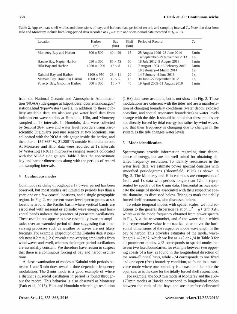
Figure 3. Power spectral density (PSD) estimates of water level (WL) at each tide gauge. Horizontal arrows indicate the frequency span of

resonant modes associated with spatial scales. Triangles mark the tidally forced shelf resonance. The red curve at Honolulu plots data from

outside the harbor.

as closed-boundary λ/2 modes. The majority of the open-

boundary condition modes correspond to transverse bay and

shelf modes, however there are exceptions, such as the 1 min

mode at Monterey and the 32 s mode at Honolulu, which are

open-boundary waves supported by open basins near the tide

gauges, as evidenced on harbor maps. We cannot assure that

all entries in Table 3 are properly attributed as λ/2 or λ/4

modes, as we have not closely examined the physical bound-

ary conditions of each mode.

5.1 Shelf resonance

The period of a shallow water wave resonance supported by a

fixed–free boundary condition is expressed in Merian’s for-

mula for an ideal open basin as T = 4L/√gd , where L is

the shelf width corresponding to λ/4, and d the basin depth

(Proudman, 1953). Similarly, a shelf resonance is dynami-

cally supported when the shelf width is approximately equal

to gα/(ω2− f 2

), where g is the gravitational acceleration,

α the shelf slope, ω the frequency of oscillation, and f the

Coriolis parameter (Clarke and Battisti, 1981). Table 4 lists

solutions for shelf-mode period (inverse of frequency) for

each of the bays, where the shelf slope is approximated as

the depth of the shelf break divided by the shelf width, and

where the basin depth is taken as one-half the shelf break

depth. Also listed are modal periods deemed to represent the

shelf resonances obtained from the power spectra in Fig. 3.

The agreement is reasonable given the simplistic formula-

Ocean Sci., 12, 355–368, 2016 www.ocean-sci.net/12/355/2016/

J. Park et. al.: Continuous seiche 361

Table 4. Estimates of shelf-resonance periods. TR is a solution to

L= gα/(ω2− f 2

), where L is the shelf width, g the gravita-

tional acceleration, α the shelf slope, ω the frequency of oscilla-

tion, and f the Coriolis parameter. The shelf slope is estimated as

break depth/width where we assume a break depth of 300 m. TM is

from Merian’s formula TM = 4L/√gd for an open basin, where d

is the basin depth which we assume to be one-half the shelf break

depth. TPSD are values from the power spectral density estimates

from shelf-mode frequencies marked with triangles in Fig. 3.

Location Latitude Width TR TM TPSD

(◦) (km) (min) (min) (min)

Monterey 36.6 15 28.9 26.1 27.4

Hawke 39.5 60 115.2 104.3 105.8

Hilo 19.7 17 32.8 29.5 30.9

Kahului 20.9 20 38.6 34.8 35.5

Mamala 21.3 15 29.0 26.1 27.1

Poverty 38.7 45 86.6 78.2 79.0

tions and crude spatial representations, and, when viewed

from the perspective of the apparently time-invariant modal

energy evident in the spectrograms and with recognition of

tidal energy as a driver of shelf resonances, suggests that

tidally forced shelf resonances are continually present.

5.2 Dynamic similarities

Topological similarities between Monterey and Hawke bays

are striking, each a semi-elliptical open bay with aspect ratios

of 2.0 and 1.9 respectively, although a factor of 2 different

in horizontal scale. One might expect that these similarities

would lead to affine dynamical behavior in terms of modal

structure, although not the specific modal resonance periods,

and that indeed appears to be the case as seen in Fig. 3. Both

bays exhibit highly tuned resonances evidenced by high qual-

ity factors (Q) in the bay modes. The shelf resonances of both

bays, 27.4 min at Monterey and 105.8 min at Hawke, indi-

cated with the triangle symbol in each plot, are exceptional

examples of this, while the longer period modes (56 min at

Monterey and 165 min at Hawke) correspond to longitudi-

nal bay oscillations. The semi-elliptical topology of these

bays is such that boundaries of the longitudinal modes are

not parallel as in an ideal rectangular basin, but are crudely

represented as semi-circular boundaries. The range of spatial

scales between these boundaries is reflected in the longitu-

dinal spectral peaks, with broad frequency spans at the base

and evidence of a series of closely spaced modes correspond-

ing to a range of wavelengths. This is contrasted to the shelf

modes where the resonances are remarkably narrow, indicat-

ing the narrow range of spatial scales reflected in the rela-

tively uniform widths of the shelves at Hawke and Monterey

Bays.

Poverty Bay is the other semi-elliptical open bay and ex-

hibits the same generic modal structure, although the bay

modes here are shorter in period due to the significantly

smaller size, and the shelf mode is the longest period mode.

It is also evident here that the shelf mode is mixed with other

modes, as it does not have a high Q factor as found at Mon-

terey and Hawke, although part of this difference could result

from poorer trapping, more radiation, or other energy loss as-

sociated with this mode.

Hilo and Kahului bays also share structural similarity, but

lack the high degree of topological symmetry found in the

semi-elliptical bays that support both longitudinal and trans-

verse modes. As is the case for the semi-elliptical bays, the

power spectra of these two bays are conspicuously similar,

with the substantial difference being the precise frequencies

of their associated modes. Here, shelf modes appear to dom-

inate the water level variance at periods less than one hour,

but rather than a set of discrete, high-Q shelf resonances

as found at Monterey and Hawke, they are energetic over a

broad range of frequencies and spatial scales. This suggests

that the shelves here are not well represented by a uniform

width, but encompass a range of scales to the shelf break, as

evidenced in bathymetric data. In the following sections we

examine specific resonance features at each of the bays.

5.3 Monterey

Monterey Bay seiching has been studied since at least the

1940s (Forston et al., 1949) with a comprehensive review

provided by Breaker et al. (2010). The primary bay modes

at the Monterey tide gauge have periods of 55.9, 36.7, 27.4,

21.8, 18.4, and 16.5 min, where the 55.9 min mode represents

the fundamental longitudinal mode, while the 36.7 min har-

monic is attributed to the primary transverse mode. We iden-

tify the 27.4 min mode as a shelf resonance, also recognized

by Lynch (1970), and consider it to be a potential continu-

ous forcing of water level oscillations throughout the bay at

periods longer than 10 min. The harbor modes (Fig. 3) have

been associated with resonances between breakwaters, and

are amplified by wave energy, whereas the bay modes are

weakly dependent on wave forcing (Park et al., 2015).

5.4 Hawke

Hawke Bay is approximately 85 km long and 45 km wide

with a rich set of modes at periods between 20 and 180 min.

Modes at periods of 170.6, 167.1, and 160.1 min correspond

to longitudinal oscillations, while the 105.8 min oscillation is

identified as a shelf resonance (Table 3).

5.5 Hilo

At Hilo we are afforded full spectral frequency coverage and

find that pier modes have periods below 20 s corresponding

to spatial scales less than 100 m. These modes are excited

by waves and swell just as the harbor modes at Monterey.

Harbor modes at periods of 3, 4, and 5.9 min correspond to

standing waves within the breakwater and spatial scales of 1,

www.ocean-sci.net/12/355/2016/ Ocean Sci., 12, 355–368, 2016

362 J. Park et. al.: Continuous seiche

1.3, and 1.9 km, respectively. The shelf offshore Hilo is not a

uniform width, but transitions from less than 2 km just south

of the bay to roughly 18 km along the northern edge, with the

spectra revealing a corresponding plateau at periods between

10 and 30 min, with a rather broad shelf resonance centered

on a period of 30.9 min, qualitatively different from the high-

Q shelf resonances at Monterey and Hawke bays. This well-

known 30.9 min mode at Hilo corresponds to a shelf reso-

nance on a shelf width of approximately 17 km.

5.6 Kahului

Oscillations at Kahului follow the same general structure as

Hilo with wave and swell excited pier modes at periods less

than 20 s, and within-harbor pier-breakwater modes at peri-

ods of 51 and 63 s. The primary harbor mode has peak en-

ergy at 188 seconds (3.1 min) corresponding to a λ/2 spatial

scale of 1.1 km, which is the dominant lateral dimension of

the harbor.

An interesting feature of the Kahului power spectra is a

low energy notch between periods of 120 and 160 s. This lack

of energy corresponds to a lack of standing wave reflective

boundaries at scales of λ/2 from 650 to 1000 m. Such low

energy features are present in all spectra indicating spatial

scales where standing waves are not supported. The domi-

nant shelf mode at Kahului has a period of 35.5 min, similar

to that of Hilo.

5.7 Honolulu

At Honolulu we have the benefit of both short sample times

(Ts = 1 s) and two gauge locations, one inside the harbor and

one on the reef outside the harbor. The offshore power spec-

trum is shown in red in Fig. 3 exemplifying an open ocean or

coastal location dominated by wind waves and swell. The re-

jection of wind wave energy inside the harbor is impressive,

revealing a set of pier modes in the 8–20 s band supported by

rectangular basins around the gauge. Modes with periods of

82 and 88 s correspond to waves with λ/2 of approximately

500 m, which is the fundamental dimension of the basin.

While the harbor is quite efficient in rejection of wind

waves and swell, amplification of the shelf mode and other

long period resonances is a striking manifestation of the “har-

bor paradox” as noted by Miles and Munk (1961). Indeed,

power spectra of the other harbors in Fig. 3 might suggest

that they may be even more efficient amplifiers.

5.8 Poverty

Poverty Bay is a small-scale version of Hawke and Monterey

bays with a similar resonance structure. However, the bay is

small enough that the lowest frequency mode is not a lon-

gitudinal mode within the bay, but is the shelf resonance at

a period of 79 min. The 57.3 min mode is not explicitly a

Poverty Bay mode, but is a longitudinal mode of the open

bay between Table Cape to the south and Gable End to the

Figure 4. Power spectral density (top) of concurrent water levels

at Napier in Hawke Bay, and Gisborne in Poverty Bay. Bottom:

coherence of the power spectra shown as the upper and lower 95 %

confidence interval values.

north, inside which Poverty Bay is inset. We also note that the

42.1 min mode is a shelf edge wave evident in both Hawke

and Poverty bays as discussed below. The reader is referred

to Bellotti et al. (2012) for a detailed numerical evaluation of

Poverty Bay shelf and bay modes.

5.9 Hawke and Poverty

Hawke and Poverty bays are located approximately 35 km

apart along the southeast coast of northern New Zealand.

Concurrent 7-month records allow examination of cross-

spectral statistics between the two locations, with power

spectra presented in the upper panel of Fig. 4 and coherence

in the lower panel plotted as the upper and lower 95 % confi-

dence intervals. Power spectra reveal that the two bays share

shallow water tidal forcings at periods longer than 180 min,

but are essentially independent in terms of major oscillation

frequencies between 20 and 180 min. There are coincident

spectral peaks near periods of 42 and 58 min; however, the

coherence of the 58 min energy is low, indicating that oscil-

lations near periods of 58 min are likely independent between

the two bays.

Coherence at the shallow water tidal periods (373, 288,

240, 199 min) is quite high and, as expected, has near zero

phase shift (not shown). Shelf modes with periods from 100

to 160 min also share coherence in the 0.5 range, which is

sensible since they have quarter wavelengths that are as long

or longer than the 35 km separation distance. The only other

energy with coherence reliably above the 0.5 range is the 42-

minute mode. This mode has a phase shift of −160◦ from

Napier (Hawke Bay) to Gisborne (Poverty Bay), indicating a

traveling wave moving from south to north along the coast,

Ocean Sci., 12, 355–368, 2016 www.ocean-sci.net/12/355/2016/

J. Park et. al.: Continuous seiche 363

empirically validating the shelf edge-wave explanation in-

ferred numerically by Bellotti et al. (2012).

6 Shelf metamodes

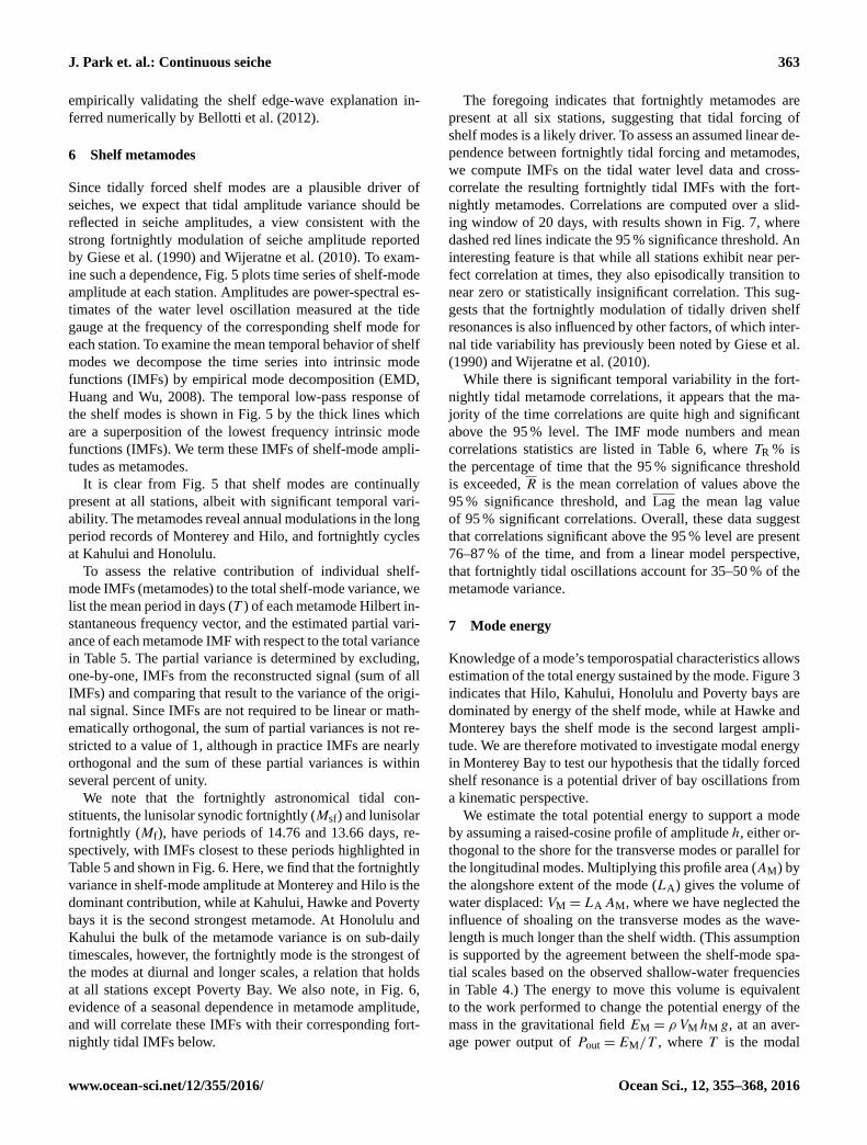
Since tidally forced shelf modes are a plausible driver of

seiches, we expect that tidal amplitude variance should be

reflected in seiche amplitudes, a view consistent with the

strong fortnightly modulation of seiche amplitude reported

by Giese et al. (1990) and Wijeratne et al. (2010). To exam-

ine such a dependence, Fig. 5 plots time series of shelf-mode

amplitude at each station. Amplitudes are power-spectral es-

timates of the water level oscillation measured at the tide

gauge at the frequency of the corresponding shelf mode for

each station. To examine the mean temporal behavior of shelf

modes we decompose the time series into intrinsic mode

functions (IMFs) by empirical mode decomposition (EMD,

Huang and Wu, 2008). The temporal low-pass response of

the shelf modes is shown in Fig. 5 by the thick lines which

are a superposition of the lowest frequency intrinsic mode

functions (IMFs). We term these IMFs of shelf-mode ampli-

tudes as metamodes.

It is clear from Fig. 5 that shelf modes are continually

present at all stations, albeit with significant temporal vari-

ability. The metamodes reveal annual modulations in the long

period records of Monterey and Hilo, and fortnightly cycles

at Kahului and Honolulu.

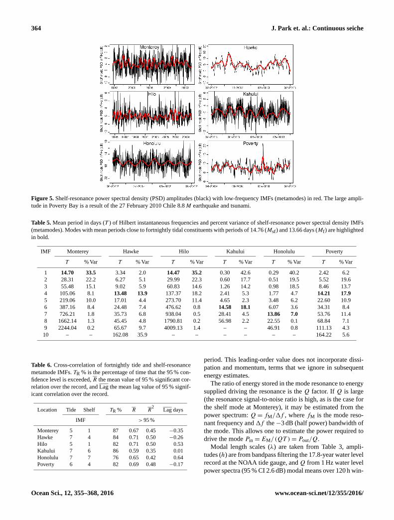
To assess the relative contribution of individual shelf-

mode IMFs (metamodes) to the total shelf-mode variance, we

list the mean period in days (T ) of each metamode Hilbert in-

stantaneous frequency vector, and the estimated partial vari-

ance of each metamode IMF with respect to the total variance

in Table 5. The partial variance is determined by excluding,

one-by-one, IMFs from the reconstructed signal (sum of all

IMFs) and comparing that result to the variance of the origi-

nal signal. Since IMFs are not required to be linear or math-

ematically orthogonal, the sum of partial variances is not re-

stricted to a value of 1, although in practice IMFs are nearly

orthogonal and the sum of these partial variances is within

several percent of unity.

We note that the fortnightly astronomical tidal con-

stituents, the lunisolar synodic fortnightly (Msf) and lunisolar

fortnightly (Mf), have periods of 14.76 and 13.66 days, re-

spectively, with IMFs closest to these periods highlighted in

Table 5 and shown in Fig. 6. Here, we find that the fortnightly

variance in shelf-mode amplitude at Monterey and Hilo is the

dominant contribution, while at Kahului, Hawke and Poverty

bays it is the second strongest metamode. At Honolulu and

Kahului the bulk of the metamode variance is on sub-daily

timescales, however, the fortnightly mode is the strongest of

the modes at diurnal and longer scales, a relation that holds

at all stations except Poverty Bay. We also note, in Fig. 6,

evidence of a seasonal dependence in metamode amplitude,

and will correlate these IMFs with their corresponding fort-

nightly tidal IMFs below.

The foregoing indicates that fortnightly metamodes are

present at all six stations, suggesting that tidal forcing of

shelf modes is a likely driver. To assess an assumed linear de-

pendence between fortnightly tidal forcing and metamodes,

we compute IMFs on the tidal water level data and cross-

correlate the resulting fortnightly tidal IMFs with the fort-

nightly metamodes. Correlations are computed over a slid-

ing window of 20 days, with results shown in Fig. 7, where

dashed red lines indicate the 95 % significance threshold. An

interesting feature is that while all stations exhibit near per-

fect correlation at times, they also episodically transition to

near zero or statistically insignificant correlation. This sug-

gests that the fortnightly modulation of tidally driven shelf

resonances is also influenced by other factors, of which inter-

nal tide variability has previously been noted by Giese et al.

(1990) and Wijeratne et al. (2010).

While there is significant temporal variability in the fort-

nightly tidal metamode correlations, it appears that the ma-

jority of the time correlations are quite high and significant

above the 95 % level. The IMF mode numbers and mean

correlations statistics are listed in Table 6, where TR % is

the percentage of time that the 95 % significance threshold

is exceeded, R is the mean correlation of values above the

95 % significance threshold, and Lag the mean lag value

of 95 % significant correlations. Overall, these data suggest

that correlations significant above the 95 % level are present

76–87 % of the time, and from a linear model perspective,

that fortnightly tidal oscillations account for 35–50 % of the

metamode variance.

7 Mode energy

Knowledge of a mode’s temporospatial characteristics allows

estimation of the total energy sustained by the mode. Figure 3

indicates that Hilo, Kahului, Honolulu and Poverty bays are

dominated by energy of the shelf mode, while at Hawke and

Monterey bays the shelf mode is the second largest ampli-

tude. We are therefore motivated to investigate modal energy

in Monterey Bay to test our hypothesis that the tidally forced

shelf resonance is a potential driver of bay oscillations from

a kinematic perspective.

We estimate the total potential energy to support a mode

by assuming a raised-cosine profile of amplitude h, either or-

thogonal to the shore for the transverse modes or parallel for

the longitudinal modes. Multiplying this profile area (AM) by

the alongshore extent of the mode (LA) gives the volume of

water displaced: VM = LAAM, where we have neglected the

influence of shoaling on the transverse modes as the wave-

length is much longer than the shelf width. (This assumption

is supported by the agreement between the shelf-mode spa-

tial scales based on the observed shallow-water frequencies

in Table 4.) The energy to move this volume is equivalent

to the work performed to change the potential energy of the

mass in the gravitational field EM = ρ VM hM g, at an aver-

age power output of Pout = EM/T , where T is the modal

www.ocean-sci.net/12/355/2016/ Ocean Sci., 12, 355–368, 2016

364 J. Park et. al.: Continuous seiche

Figure 5. Shelf-resonance power spectral density (PSD) amplitudes (black) with low-frequency IMFs (metamodes) in red. The large ampli-

tude in Poverty Bay is a result of the 27 February 2010 Chile 8.8M earthquake and tsunami.

Table 5. Mean period in days (T ) of Hilbert instantaneous frequencies and percent variance of shelf-resonance power spectral density IMFs

(metamodes). Modes with mean periods close to fortnightly tidal constituents with periods of 14.76 (Msf) and 13.66 days (Mf) are highlighted

in bold.

IMF Monterey Hawke Hilo Kahului Honolulu Poverty

T % Var T % Var T % Var T % Var T % Var T % Var

1 14.70 33.5 3.34 2.0 14.47 35.2 0.30 42.6 0.29 40.2 2.42 6.2

2 28.31 22.2 6.27 5.1 29.99 22.3 0.60 17.7 0.51 19.5 5.52 19.6

3 55.48 15.1 9.02 5.9 60.83 14.6 1.26 14.2 0.98 18.5 8.46 13.7

4 105.06 8.1 13.48 13.9 137.37 18.2 2.41 5.3 1.77 4.7 14.21 17.9

5 219.06 10.0 17.01 4.4 273.70 11.4 4.65 2.3 3.48 6.2 22.60 10.9

6 387.16 8.4 24.48 7.4 476.62 0.8 14.58 18.1 6.07 3.6 34.31 8.4

7 726.21 1.8 35.73 6.8 938.04 0.5 28.41 4.5 13.86 7.0 53.76 11.4

8 1662.14 1.3 45.45 4.8 1790.81 0.2 56.98 2.2 22.55 0.1 68.84 7.1

9 2244.04 0.2 65.67 9.7 4009.13 1.4 – – 46.91 0.8 111.13 4.3

10 – – 162.08 35.9 – – – – – – 164.22 5.6

Table 6. Cross-correlation of fortnightly tide and shelf-resonance

metamode IMFs. TR % is the percentage of time that the 95 % con-

fidence level is exceeded, R the mean value of 95 % significant cor-

relation over the record, and Lag the mean lag value of 95 % signif-

icant correlation over the record.

Location Tide Shelf TR % R R2

Lag days

IMF > 95 %

Monterey 5 1 87 0.67 0.45 −0.35

Hawke 7 4 84 0.71 0.50 −0.26

Hilo 5 1 82 0.71 0.50 0.53

Kahului 7 6 86 0.59 0.35 0.01

Honolulu 7 7 76 0.65 0.42 0.64

Poverty 6 4 82 0.69 0.48 −0.17

period. This leading-order value does not incorporate dissi-

pation and momentum, terms that we ignore in subsequent

energy estimates.

The ratio of energy stored in the mode resonance to energy

supplied driving the resonance is the Q factor. If Q is large

(the resonance signal-to-noise ratio is high, as is the case for

the shelf mode at Monterey), it may be estimated from the

power spectrum: Q= fM/1f , where fM is the mode reso-

nant frequency and1f the−3 dB (half power) bandwidth of

the mode. This allows one to estimate the power required to

drive the mode Pin = EM/(QT )= Pout/Q.

Modal length scales (λ) are taken from Table 3, ampli-

tudes (h) are from bandpass filtering the 17.8-year water level

record at the NOAA tide gauge, andQ from 1 Hz water level

power spectra (95 % CI 2.6 dB) modal means over 120 h win-

Ocean Sci., 12, 355–368, 2016 www.ocean-sci.net/12/355/2016/

J. Park et. al.: Continuous seiche 365

Figure 6. Intrinsic mode functions (IMF) of shelf-mode amplitude variance (metamodes) with mean Hilbert instantaneous frequencies

corresponding to fortnightly periods (highlighted in Table 5). Amplitudes are with respect to the mean values shown in Fig. 5. Records at

Honolulu and Kahului are limited to 3 months, while the other stations show excerpts of approximately 13 months.

Figure 7. Correlation coefficients between tide and shelf-resonance metamode IMFs with fortnightly periods. The dashed red lines indicate

the 95 % confidence levels.

dows over 63 days (Park et al., 2015). The alongshore ex-

tent of the modes, LA, is estimated from a regional ocean

modeling system (ROMS) implementation in Monterey Bay

(Shchepetkin and McWilliams, 2005) as reported in Breaker

et al. (2010).

Results of these estimates are shown in Table 7, where we

find seiche amplitudes averaged over the 17.8-year period of

0.9, 1.4, and 1.6 cm for the 55.9, 27.4, and 36.7 min modes,

respectively, although amplitudes of 4 cm in the 27.4 min

mode are common during seasonal maximums. The 27.4 min

shelf mode is estimated to produce a total power of 998 kW,

www.ocean-sci.net/12/355/2016/ Ocean Sci., 12, 355–368, 2016

366 J. Park et. al.: Continuous seiche

Table 7. Estimates of total energy and power generated by resonances in Monterey Bay. Modal amplitudes (h) are mean values from bandpass

filtering the 17.8-year record of water levels at the NOAA tide gauge. T is the mode period, WFIR is the filter bandpass, λ/2 the mode half

wavelength, LA the alongshore extent of the mode in the bay, V the volume of water displaced, EM the potential energy, Q the mode

amplification, Pin = EM/(QT ) the input driving power of the mode, and Pout = EM/T the modal power.

T WFIR h λ/2 LA V EM Q Pin Pout

(min) (min) (cm) (km) (km) (Mm3) (GJ) (kW) (kW)

27.4 25–30 1.4 31.6 38 33.30 1.64 12.9 77.6 998.1

36.7 35–39 1.6 42.2 40 52.55 2.91 7.8 168.6 1319.7

55.9 53–59 0.9 40.7 18 13.27 0.43 5.6 22.7 127.3

which is more than sufficient to supply the required in-

put power of both the primary longitudinal (55.9 min, Pin =

23 kW) and transverse (36.7 min, Pin = 169 kW) bay modes.

So even though the primary longitudinal bay modes in both

Monterey and Hawke bays have larger amplitudes than the

respective shelf modes, the shelf mode in Monterey supplies

a continuous source of energy capable of sustaining the fun-

damental bay modes, which by virtue of their resonant am-

plification can exceed the amplitude of the shelf resonance it-

self. Regarding the low-frequency infragravity waves of mil-

limeter amplitude suggested by MacMahan (2015), we note

that a 27.4 min mode with an amplitude of 3 mm would pro-

duce an estimated Pout of 41.6 kW (not shown in Table 7),

which would be insufficient to drive the observed 27.4 min

mode as it requires a power of Pin = 77 kW.

8 Discussion

Resonant modes are a fundamental physical characteristic of

bounded physical systems expressed in bodies of water as

seiches. As such, they can be excited to large amplitudes

by transitory phenomena such as weather and tsunamis, and

since large amplitude seiches are easily observable, seiches

are often viewed as transitory given that they dissipate after

cessation of the driving force. Moving from transient to per-

sistent behavior, seasonal weather patterns are known to sus-

tain nearly continuous seiching for extended periods (Wood-

worth et al., 2005; Wijeratne et al., 2010), as internal waves

are also known to do (Giese et al., 1990). On the other hand,

small amplitude, temporally continuous seiches were recog-

nized by Cartwright and Young (1974) and Golmen et al.

(1994), with Giese and Chapman (1993) and Breaker et al.

(2010) posing questions as to the possibility of global excita-

tions. Motivated by these questions, we have examined tide

gauge water levels around the Pacific basin, looking for con-

tinuous seiching and forcings.

In the process of analyzing the resonant structure of these

bays and harbors, we have quantified resonant periods and

estimated spatial scales corresponding to each mode (Ta-

ble 3). In some cases, we have identified the physical at-

tributes of a bay or harbor associated with specific tem-

porospatial resonances. In a more general sense, we have also

illustrated broad dynamical similarities between bays with

affine topologies, such as the clearly defined modes of the

semi-elliptical bays when compared to the less structured,

shelf-dominated bays such as Hilo and Kahului. This anal-

ysis also provides empirical verification of the numerically

inferred edge wave by Bellotti et al. (2012) near a period of

42 min along Hawke and Poverty bays.

Simple geometric and dynamical estimates of tidally

forced shelf modes are consistent with modes observed in

the power spectra at all stations, and their continual pres-

ence in water level spectrograms and mode amplitude time

series indicates that tidally forced shelf modes are continu-

ously present at each location. Decomposition of shelf-mode

amplitude time series identifies metamodes reflecting dy-

namic behavior of the shelf modes, and we find that fort-

nightly metamodes are the dominant mode at periods longer

than diurnal. Assuming that these fortnightly modulations

are of tidal origin, cross-correlation of fortnightly IMFs of

tidal data with the fortnightly metamodes leads to the con-

clusion that within the bounds of a linear system model from

one-third to one-half of the fortnightly metamode variance is

coherent with tidal forcing. We therefore suspect that tidally

forced shelf modes are a continuous energy source in harbors

and bays adjacent to continental or island shelves.

However, it is also clear that we do not understand the

cyclic nature of fortnightly tidal and metamode correlation.

One possibility is that there is a time-varying phase lag be-

tween the two such that destructive superposition episodi-

cally creates nulls. A linear spectral analysis might use a

coherency statistic to identify this, but such an option is

not available for IMFs with variable instantaneous frequen-

cies. It is evident that internal tides play a role, and it may

be that episodic changes in stratification as noted by Giese

et al. (1990) lead to modulation of the metamodes and con-

tribute to the observed decorrelation, and it is deemed likely

that the free, long-frequency infragravity waves suggested by

MacMahan (2015) also contribute.

A natural question is: does the proposed source contain

sufficient energy to sustain the observed resonant oscillation?

Power estimates of the most energetic modes at Monterey

suggest that the shelf mode is fully capable as a primary

driver of continuous seiche, while the low-frequency infra-

Ocean Sci., 12, 355–368, 2016 www.ocean-sci.net/12/355/2016/

J. Park et. al.: Continuous seiche 367

gravity waves suggested by MacMahan (2015) may not have

sufficient energy.

9 Conclusions

Examination of six coastal locations around the Pacific with

diverse shelf conditions finds that tidally forced shelf reso-

nances are continually present. An energy assessment of the

shelf mode and primary seiche in Monterey Bay indicates

that the shelf resonance is fully capable of supplying the

power input required to drive the primary bay oscillations,

even though the grave mode produces more output power

than the shelf mode, a consequence of the resonance struc-

ture of the bay. Hawke Bay is dynamically similar to Mon-

terey and we suspect that a similar relation holds there, while

at the other locations the shelf mode is the dominant energy

source. Our conclusion is that tidally forced shelf modes con-

stitute a global candidate for continuous seiche excitation,

a view consistent with that of Lynch (1970), Golmen et al.

(1994), and Wijeratne et al. (2010), who identified tidally

forced shelf resonances as specific seiche modes. In loca-

tions where tidally forced shelf resonance is a primary seiche

generator, we suspect that internal waves and weather, which

clearly can be a primary forcing in their own right, serve to

modulate seiche amplitudes.

Specific to Monterey Bay, these results offer a sim-

pler explanation for continuous seiche generation than the

mesoscale gyre hypothesis proposed by Park et al. (2015),

which lacked a physical mechanism to transfer energy into

the bay, and is more energetically reasonable than the infra-

gravity waves suggested by MacMahan (2015).

In the course of attributing tidal forcing as the driver of

the observed shelf resonances, we introduced the idea of

metamodes, dynamical modes of shelf-mode amplitude de-

termined by empirical mode decomposition. The metamodes

exhibited fortnightly modulation, and it is likely that exami-

nation of other metamode components may be useful towards

understanding the dynamic behavior of modal structure in

coastal environments.

Acknowledgements. We are indebted to Lawrence Breaker of Moss

Landing Marine Laboratory for his identification of continuous

seiche in Monterey Bay, his questioning of their origin, and fruitful

discussions. We gratefully acknowledge additional citations on

continuous seiche provided by an anonymous reviewer.

Edited by: J. M. Huthnance

References

Airy, G. B.: On the Tides at Malta, Philos. T. ROY. SOC., 169, 123–

138, 1877.

Bellotti, G., Briganti, R., and Beltrami, G. M.: The combined role

of bay and shelf modes in tsunami amplification along the coast,

J. Geophys. Res., 117, C08027, doi:10.1029/2012JC008061,

2012.

Bloomfield, P.: Fourier Analysis of Time Series: An Introduction,

1st Edn., Wiley, New York, 261 pp., 1976.

Breaker, L. C., Broenkow, W. W., Watson, W. E., and Jo, Y.: Tidal

and non-tidal oscillations in Elkhorn Slough, California, Estuar.

Coast., 31, 239–257, 2008.

Breaker, L. C., Tseng, Y., and Wang, X.: On the natural oscillations

of Monterey Bay: observations, modeling, and origins, Prog.

Oceanogr., 86, 380–395, doi:10.1016/j.pocean.2010.06.001,

2010.

Cartwright, D. E. and Young, M. Y.: Seiches and tidal ringing in

the sea near Shetland, P. Roy. Soc. Lond. A Mat., 338, 111–128,

1974.

Chrystal, G.: On the hydrodynamical theory of seiches, T. Roy. Soc.

Edin.-Earth, 41, 599–649, doi:10.1017/S0080456800035523,

1906.

Clarke, A. J. and Battisti, D. S.: The effect of continental shelves on

tides, Deep-Sea Res., 28, 665–682, 1981.

Darwin, G. H.: The Tides and Kindred Phenomena in the Solar Sys-

tem, Houghton, Boston, 1899.

Forston, E. P., Brown, F. R., Hudson, R. Y., Wilson, H. B., and Bell,

H. A.: Wave and surge action, Monterey Harbor, Monterey Cal-

ifornia, Tech. Rep. 2-301, United States Army Corps of Engi-

neers, Waterways Experiment Station, Vicksburg, MS, 45 Plates,

1949.

Giese, G. S. and Chapman, D. C.: Coastal seiches, Oceanus, 36,

38–46, 1993.

Giese, G. S., Chapman, D. C., Black, P. G., and Fornshell, J. A.:

Causation of large-amplitude coastal seiches on the Carribbean

coast of Puerto Rico, J. Phys. Oceanogr., 20, 1449–1458, 1990.

Giese, G. C., Chapman, D. C., Collins, M. G., Encarna-

cion, R., and Jacinto, G.: The coupling between har-

bor seiches at palawan island and sulu sea internal soli-

tons, J. Phys. Oceanogr., 28, 2418–2426, doi:10.1175/1520-

0485(1998)028<2418:TCBHSA>2.0.CO;2, 1998.

Golmen, L. G., Molvir, J., and Magnusson, J.: Sea level oscilla-

tions with super-tidal frequency in a coastal embayment of west-

ern Norway, Cont. Shelf Res., 14, 1439–1454, doi:10.1016/0278-

4343(94)90084-1, 1994.

Huang, N. E. and Wu, Z.: A review on Hilbert–Huang transform:

method and its applications to geophysical studies, Rev. Geo-

phys., 46, RG2006, doi:10.1029/2007RG000228, 2008.

Lowry, R., Pugh, D. T., and Wijeratne, E. M. S.: Observations of

Seiching and Tides Around the Islands of Mauritius and Ro-

drigues, Western Indian Ocean Journal of Marine Science, 7, 15–

28, 2008.

Lynch, T. J.: Long Wave Study of Monterey Bay, MS thesis,

Naval Postgraduate School, Monterey, California, avail-

able at: calhoun.nps.edu/bitstream/handle/10945/15072/

longwavestudyofm00lync.pdf (last access: 3 March 2016),

1970.

www.ocean-sci.net/12/355/2016/ Ocean Sci., 12, 355–368, 2016

368 J. Park et. al.: Continuous seiche

MacMahan, J.: Low-Frequency Seiche in a Large Bay., J. Phys.

Oceanogr., 45, 716–723, doi:10.1175/JPO-D-14-0169.1, 2015.

Miles, J. and Munk, W.: Harbor paradox, J. Waterways Div.-ASCE,

87, 111–132, 1961.

Okihiro, M. and Guza, R. T.: Observation of seiche forcing and am-

plification in three small harbors, J. Waterw. Port C.-ASCE, 122,

232–238, 1996.

Park, J., Sweet, W. V., and Heitsenrether, R.: Water level oscilla-

tions in Monterey Bay and Harbor, Ocean Sci., 11, 439–453,

doi:10.5194/os-11-439-2015, 2015.

Proudman, J.: Dynamical Oceanography, Methuen, London; Wiley,

New York, 409 pp., 1953.

Rabinovich, A. B.: Seiches and Harbor Oscillations, in: Handbook

of Coastal and Ocean Engineering, edited by: Young, C. K.,

World Scientific, Singapore, 193–236, 2009.

Shchepetkin, A. F. and McWilliams, J. C.: The regional

oceanic modeling system (ROMS): a split-explicit, free-surface,

topography-following-coordinate oceanic model, Ocean Model.,

9, 347–404, doi:10.1016/j.ocemod.2004.08.002, 2005.

Taylor, G. I.: Tidal Friction in the Irish Sea, P. Roy. Soc. A-Math.

Phy., 96, 330–330, doi:10.1098/rspa.1919.0059, 1919.

Thotagamuwage, D. T. and Pattiaratchi, C. B.: Influence of offshore

topography on infragravity period oscillations in Two Rocks Ma-

rina, Western Australia, Coast. Eng., 91, 220–230, 2014.

Webb, D. J.: A model of continental-shelf resonances, Deep-Sea

Res., 23, 1–15, 1976.

Wijeratne, E. M. S., Woodworth, P. L., and Pugh, D. T.:

Meteorological and internal wave forcing of seiches along

the Sri Lanka coast, J. Geophys. Res., 115, C03014,

doi:10.1029/2009JC005673, 2010.

Woodworth, P. L., Pugh, D. T., Meredith, M. P., and Blackman,

D. L.: Sea level changes at Port Stanley, Falkland Islands, J. Geo-

phys. Res., 110, C06013, doi:10.1029/2004JC002648, 2005.

Ocean Sci., 12, 355–368, 2016 www.ocean-sci.net/12/355/2016/