Embed Size (px)
Citation preview
Continuous Obstructed Nearest Neighbor Queries in Spatial Databases
Yunjun Gao
School of Information Systems Singapore Management University
Baihua Zheng School of Information Systems
Singapore Management University [email protected]
ABSTRACT In this paper, we study a novel form of continuous nearest neighbor queries in the presence of obstacles, namely continuous obstructed nearest neighbor (CONN) search. It considers the impact of obstacles on the distance between objects, which is ignored by most of spatial queries. Given a data set P, an obstacle set O, and a query line segment q in a two-dimensional space, a CONN query retrieves the nearest neighbor of each point on q according to the obstructed distance, i.e., the shortest path between them without crossing any obstacle. We formulate CONN search, analyze its unique properties, and develop algorithms for exact CONN query processing, assuming that both P and O are indexed by conventional data-partitioning indices (e.g., R-trees). Our methods tackle the CONN retrieval by performing a single query for the entire query segment, and only process the data points and obstacles relevant to the final result, via a novel concept of control points and an efficient quadratic-based split point computation algorithm. In addition, we extend our solution to handle the continuous obstructed k-nearest neighbor (COkNN) search, which finds the k (≥ 1) nearest neighbors to every point along q based on obstructed distances. A comprehensive experimental evaluation using both real and synthetic datasets has been conducted to demonstrate the efficiency and effectiveness of our proposed algorithms.
Categories and Subject Descriptors H.2.8 [Database Management]: Database Applications ⎯ Spatial databases and GIS; H.2.4 [Database Management]: Systems ⎯ Query processing
General Terms Algorithms, Design, Experimentation, Performance, Theory
Keywords Nearest neighbor, Continuous nearest neighbor, Continuous obstructed nearest neighbor, Spatial database, Obstacle
1. INTRODUCTION With the growing popularity of smart mobile devices (e.g.,
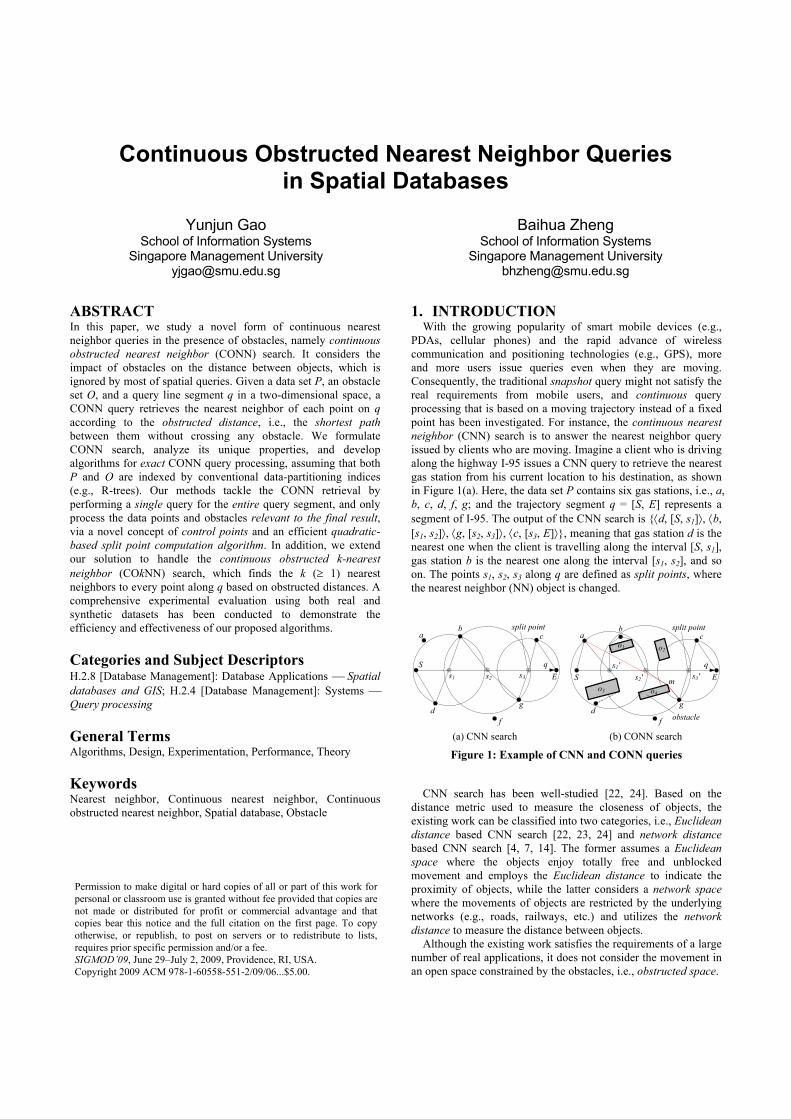
PDAs, cellular phones) and the rapid advance of wireless communication and positioning technologies (e.g., GPS), more and more users issue queries even when they are moving. Consequently, the traditional snapshot query might not satisfy the real requirements from mobile users, and continuous query processing that is based on a moving trajectory instead of a fixed point has been investigated. For instance, the continuous nearest neighbor (CNN) search is to answer the nearest neighbor query issued by clients who are moving. Imagine a client who is driving along the highway I-95 issues a CNN query to retrieve the nearest gas station from his current location to his destination, as shown in Figure 1(a). Here, the data set P contains six gas stations, i.e., a, b, c, d, f, g; and the trajectory segment q = [S, E] represents a segment of I-95. The output of the CNN search is {⟨d, [S, s1]⟩, ⟨b, [s1, s2]⟩, ⟨g, [s2, s3]⟩, ⟨c, [s3, E]⟩}, meaning that gas station d is the nearest one when the client is travelling along the interval [S, s1], gas station b is the nearest one along the interval [s1, s2], and so on. The points s1, s2, s3 along q are defined as split points, where the nearest neighbor (NN) object is changed.
s1 s2 s3 E
ab
c
df
g
split point
S q
S E
ab
c
df
g
o3
o1 o2
o4
obstacle
split point
qs2' s3'm
s1'
(a) CNN search (b) CONN search
Figure 1: Example of CNN and CONN queries
CNN search has been well-studied [22, 24]. Based on the distance metric used to measure the closeness of objects, the existing work can be classified into two categories, i.e., Euclidean distance based CNN search [22, 23, 24] and network distance based CNN search [4, 7, 14]. The former assumes a Euclidean space where the objects enjoy totally free and unblocked movement and employs the Euclidean distance to indicate the proximity of objects, while the latter considers a network space where the movements of objects are restricted by the underlying networks (e.g., roads, railways, etc.) and utilizes the network distance to measure the distance between objects.
Although the existing work satisfies the requirements of a large number of real applications, it does not consider the movement in an open space constrained by the obstacles, i.e., obstructed space.
Permission to make digital or hard copies of all or part of this work for personal or classroom use is granted without fee provided that copies are not made or distributed for profit or commercial advantage and that copies bear this notice and the full citation on the first page. To copy otherwise, or republish, to post on servers or to redistribute to lists, requires prior specific permission and/or a fee. SIGMOD’09, June 29–July 2, 2009, Providence, RI, USA. Copyright 2009 ACM 978-1-60558-551-2/09/06...$5.00.
For example, a battlefield usually does not have any fixed road network structure and tanks/soldiers can move totally free, as long as the path is not blocked. Another example is that mobile robots help rescue survivors after a disaster (e.g., a devastating earthquake). The robots equipped with location-sensing ability as well as visual and other sensors can burrow into the rubble and try to locate potential survivors, which can facilitate the excavation without further injuring survivors. Theoretically, the robot navigating the space can take any direction but the physical obstacles (e.g., rocks etc.) affect the real distance that a robot has to travel in order to reach its destination.
Consequently, the obstructed space is different from both the Euclidean space and the network space. Compared with the Euclidean space, it considers the existence of obstacles that may block the immediate path from one object to another and hence the Euclidean distance between them does not always indicate the real travelling distance. On the other hand, compared with the network space, it does not assume any underlying fixed network structure and still entitles the objects to free movements. Correspondingly, the distance between two objects in an obstructed space is measured based on the obstructed distance, i.e., the shortest path connecting two objects without crossing any obstacle. Take the objects a and g shown in Figure 1(b) as an example. Their Euclidean distance is the length of segment [a, g], whereas their obstructed distance is the summation of the lengths of segment [a, m] and segment [m, g], because of the obstruction of obstacle o4.
In this paper, we consider the CNN search in an obstructed space, namely continuous obstructed nearest neighbor (CONN) search. Given a data set P, an obstacle set O, and a query line segment q in a two-dimensional (2D) space, a CONN query retrieves the obstructed nearest neighbor (ONN) for every point along q according to the obstructed distance. Specifically, the CONN retrieval aims at finding a set of ⟨p, R⟩ tuples, where p ∈ P is the ONN for any point in the interval R ⊆ q. Continuing the example in Figure 1(b) where the obstacle set O contains four rectangular obstacles1 o1, o2, o3, and o4, the CONN query returns {⟨a, [S, s1′]⟩, ⟨b, [s1′, s2′]⟩, ⟨g, [s2′, s3′]⟩, ⟨c, [s3′, E]⟩}, which indicates that object a is the ONN for each point along interval [S, s1′], object b is the ONN for each point along interval [s1′, s2′], etc. Note that the split points s1, s2, and s3 defined by a CNN search are different from the split points s1′, s2′, and s3′ defined by a CONN search. In addition, the answer objects vary as well. For example, object d is the NN for S in a Euclidean space, whereas it is not the ONN for S in an obstructed space, due to the blocking of obstacle o3.
CONN search is useful for many real-life applications. Consider the example of robots rescuing survivors. Suppose that the robots successfully locate some survivors and a 3D map has been constructed based on the data collected by robots along their way navigating the space. Based on the map information, we can identify several routes that are not blocked and invoke CONN search to locate the nearest survivors along the path. The number of nearest survivors and the distance between the survivors to the corresponding points along the path provide critical information that can help the emergency personnel to plan the excavation. We focus this paper on the CONN query, not only because the
1 Although an obstacle can be in any shape (e.g., triangle,
pentagon, etc.), we assume it is a rectangle in this paper.
problem is interesting and has a large application base, but also because it poses some challenging research issues that are worth investigating.
The first issue is how to calculate the obstructed distance efficiently. Based on the existing work related to robot motion planning, the lower bound of the calculation is O (nlogn), with n as the total number of obstacle vertices [2]. In practice, a popular and practical method based on visibility graph VG [2] has O (n2 logn) as the worst case time complexity. Compared with Euclidean distance which can be derived in constant time, the computation cost of the obstructed distance is much more expensive. In addition, VG-based approaches need to maintain a visibility graph, which requires O (n2) space in the worst case. The high space complexity deteriorates its scalability, not to mention its extremely high update cost.
We try to tackle this issue from two aspects, i.e., reducing the number of obstructed distance calculations and simplifying the obstructed distance calculations. The former objective is achieved via effective pruning techniques that can filter out unqualified objects as early as possible. As for the second target, we construct a local visibility graph to simplify the calculation process. Initially, the local visibility graph only contains two endpoints of a given query line segment. As we process the query and evaluate data points, we incrementally insert the obstacles that might affect the query result into the local visibility graph. Due to the small size of the local visibility graph, the insertion/deletion/update can be efficiently supported.
The second issue is how to efficiently answer a CONN query. A naive approach is to issue an obstructed nearest neighbor (ONN) search [31] at every point of a specified query line segment q. However, this approach is definitely infeasible as the number of points on q is infinite. Motivated by the fact that nearby points along the query segment might share the same ONN, we adopt an incremental approach to fine-tune the result upon the evaluation of each new data point, based on the concept of split point (i.e., the points along the query segment bounded by two continuous split points share the same ONN). Nevertheless, due to the existence of obstacles, existing split point formation algorithms developed for CNN search cannot be applied. In this paper, we propose a novel concept, namely control point, to facilitate the computation of obstructed distances, and design a quadratic-based approach to form split points. In addition, several pruning strategies have been proposed to further improve the search performance.
In summary, this paper has made five-fold main contributions, summarized as follows:
We formalize CONN search, a new addition to the family of spatial queries in an obstructed space. To the best of our knowledge, this paper is the first attempt on this problem.
We introduce the concept of control point that significantly simplifies the computation and comparison of the obstructed distance between two objects.
We propose a quadratic-based method to form split points, by solving quadratic inequalities.
We develop an efficient algorithm for processing CONN search which can be extended to handle COkNN retrieval.
We conduct extensive experiments using both real and synthetic datasets to demonstrate the efficiency and effectiveness of the proposed algorithms.
The rest of this paper is organized as follows. Section 2 overviews related work. Section 3 formulates the CONN problem, introduces the concept of control point, and presents the split point computation approach. Section 4 elaborates an efficient algorithm for CONN query. Section 5 reports experimental results and our findings. Finally, Section 6 concludes the paper with some directions for future work.
2. RELATED WORK In this section, we review the existing work related to CONN
queries, namely, point NN search in the Euclidean space, snapshot CNN/CkNN queries, query processing with the existence of obstacles, and main-memory obstacle path search.
2.1 Point NN Search A conventional (i.e., point) NN query finds the k (≥ 1) data
point(s) from a data set that are closest to a specified query point q according to Euclidean distance. The algorithms for NN search on R-trees [1, 11, 19] follow the branch-and-bound paradigm and utilize some metrics to prune the search space. For example, the metric mindist(q, N) corresponds to the minimal distance between q and any point included by a node N; and thus it gives a lower bound of the distance from any point of N to q.
Existing algorithms for NN search usually follow either best-first (BF) or depth-first (DF) traversal paradigm. DF algorithms [3, 18] start from the root, and visit recursively the node with the smallest mindist to q until the leaf level where a potential NN is reached. Subsequently, the algorithm conducts backtrackings. In particular, during backtracking to the upper levels, DF only visits those entries whose minimum distances to q are smaller than the distance between the NN candidate retrieved so far and the query point. As demonstrated in [16], the DF algorithm is suboptimal, i.e., it accesses more nodes than necessary.
BF algorithms [12, 13] achieve the optimal I/O performance by visiting only the nodes necessary for obtaining the NN(s). Towards this, BF maintains a heap H with the entries visited so far, sorted in ascending order of their mindist to q. Starting from the root node, BF recursively examines the top entry e of H. If e is an intermediate node (i.e., a non-leaf node), its child entries are en-heaped for later examination. If e is a data point, it is reported as an actual NN of a query point. Both DF and BF can be easily extended to retrieve k (> 1) NNs. Furthermore, BF is incremental, i.e., it returns the NNs in ascending order of their distances to the query point; and hence k does not have to be known in advance, which allows different termination conditions to be applied.
2.2 Snapshot CNN/CkNN Queries The CNN search has received considerable attention since it
was first introduced by Sistla et al. [21] in spatial-temporal databases. In the initial work, modeling methods and query languages for the expression of CNN queries are presented, but not the processing algorithms. The first algorithm for CNN query processing, based on periodical sampling technique, is proposed in [22]. Due to the inherent shortcoming of sampling, its performance highly depends on the number and positions of those sampling points and its accuracy cannot be guaranteed. In order to conduct exact CNN search, two query processing algorithms are proposed in [23, 24], using R-trees as the underlying data structure. The first algorithm is based on the concept of time-parameterized (TP) queries [23], which treats a query line segment as the moving trajectory of a query point. Thus, the
nearest object to the moving query point is valid only for a limited duration, and a new TP query is issued to retrieve the next nearest object once the valid time of current query expires, i.e., when a split point is reached. Although the TP approach avoids the drawbacks of sampling, it needs to issue m TP queries with m the number of answer objects. In order to improve the performance, the second algorithm [24] retrieves all the answer objects for the whole query line segment in a single round. Recently, Zheng et al. [32] study CNN search in wireless data broadcast systems, where mobile clients answer their own CNN search via listening to the wireless broadcast channel.
All the above work on CNN queries use Euclidean distances to measure the proximity of objects. As for network distance, the first algorithm to process CNN queries in a road network is proposed in [7], which tries to find the locations on a path that an NN search must be performed. However, it does not support CkNN search. Motivated by this, Kolahdouzan and Shahabi [14] present two methods, namely, Intersection Examination (IE) and Upper Bound Algorithm (UBA). Compared with IE, UBA gains better performance by restricting the evaluation of kNN queries to only the locations where they are required. An alternative approach is proposed in [4]. It retrieves the kNN object sets of all network nodes in the query path, and associates them with the data objects located along the path.
As mentioned in Section 1, all the aforementioned algorithms do not take into consideration the existence of obstacles and they cannot be used to deal with CONN queries efficiently. The main difference between CNN search and CONN search has been summarized in [31].
2.3 Queries with Obstacles In an obstructed space, the distance between objects is affected
by the existence of physical obstacles (e.g., buildings, rivers, etc.). Zhang et al. [31] propose several algorithms for processing common spatial queries such as range queries, NN search, e-distance join queries, closest pair queries and distance semi-join queries, in the obstructed space. Xia et al. [29] present a more detailed study of the obstructed nearest neighbor (ONN) query which finds the k (≥ 1) NNs of a given query point according to the obstructed distance. However, to the best knowledge of the authors, the CONN search has not been studied before.
More recently, the impact of obstacles on the object visibility has been studied. Although it does not employ the obstructed distance to measure the closeness between objects, it does consider the existence of obstacles and two objects are visible to each other iff the straight line segment connecting them does not pass through any obstacle. Nutanong et al. [15] explore the visible k-nearest neighbor (VkNN) search, which returns the k NNs that are visible to a specified query point. Further studies along this line include visible reverse k-nearest neighbor search [8] and continuous VkNN search [9].
In addition, the problem of spatial clustering in the presence of obstacles has attracted considerable attention in recent years. It divides a set of 2D data points into smaller homogeneous groups (i.e., clusters) by taking into account the influence of obstacles. Handling these constraints can lead to effective and fruitful data mining by capturing application semantics [26]. A large number of clustering algorithms with obstacle constraints have been proposed in the literature, including COD_CLARANS [25], AUTOCLUST+ [6], DBCLuC [30], DBRS+ [28], DBRS_O [27], and DBSCAN_MDO [17], etc.

2.4 Main-Memory Obstacle Path Queries Main-memory based shortest path problem in the presence of
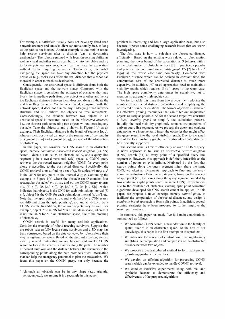
obstacles has been well-studied in computational geometry [2], and the most common approach is based on the visibility graph VG. A VG is constructed based on an obstacle set O and the source/destination point ps/pe. Its nodes correspond to the vertices of the obstacles or source/destination point. Two nodes ni, nj are connected iff the straight line segment between them does not intersect any obstacle interior.
ps
pe
obstacle
the shortest pathn1
n2
n3n4
o1o2
n5 n6
n8 n7 Figure 2: Visibility graph and obstacle path
An example VG is illustrated in Figure 2, where shaded
polygons represent obstacles. Nodes n2 and n7 are not connected as the corresponding straight line segment [n2, n7] intersects with the obstacle o2. There are multiple paths available from the source point ps to the destination point pe, such as the path via nodes n1, n6 and the path via nodes n1, n8, and n7. Among all the available paths, the one with the shortest distance is returned, i.e., the path via nodes n4, n3, n5 and n6 for this example. Since the shortest path contains only the edges of VG (as proved in [2]), a popular and practical obstacle path (i.e., shortest path) computation approach proceeds in two steps. The first step constructs VG, which takes O (n2 logn) based on rotational plane sweep [20], and can be optimized to O (m + n logn) with an optimal output-sensitive algorithm [10]. Here, n is the number of nodes in VG and m is the number of edges in VG. The second step computes the shortest path in VG using Dijkstra’s algorithm [5], which incurs O (m + n logn). Thus, the time and space complexities of the approach are O (n2 logn) and O (n2), respectively. Obviously, the algorithm has a poor scalability and cannot guarantee the efficiency when a large number of obstacles are considered.
3. PRELIMINARIES In this section, we formally define CONN search, introduce the
concept of control points, and present the quadratic-based split point computation algorithm that is crucial to CONN query processing. Table 1 summarizes the notations used in the rest of this paper.
Table 1. Symbols and descriptions Notation Description P the set of data points p in a 2D space O the set of obstacles o in a 2D space Tp the R-tree on P To the R-tree on O q the query line segment with q = [S, E] VG the visibility graph RL the result list of a CONN query dist(pi, pj) the Euclidean distance between pi and pj H.head the top entry of a heap H e.key the search key value of a heap entry e
DEFINITION 1 (VISIBILITY [8]). Given p, p′ ∈ P and O, p and p′ are visible to each other iff the straight line connecting them does not cut through any obstacle, i.e., ∀ o ∈ O, [p, p′] ∩ o = ∅. □
DEFINITION 2 (VISIBLE REGION). Given p ∈ P, O, and q, the visible region of p over q, denoted by VRp,q, is the set of intervals R ⊆ q, such that p is visible to all the points along R. □
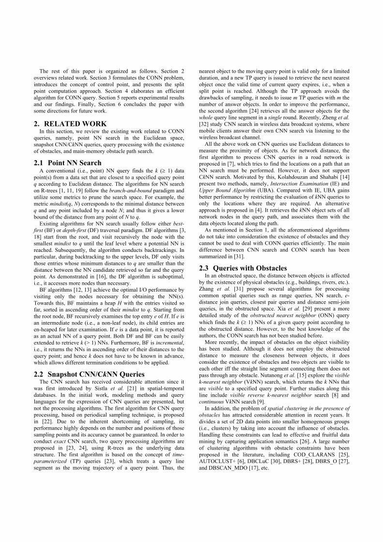
In a Euclidean space, any two points are visible to each other as there are no obstacles. However, this statement does not hold in an obstructed space. As shown in Figure 3, the visible region of p over q is [S, s1], and the rest (i.e., the segment [s1, E]) is blocked by obstacles o1 and/or o2. Point s2 is not located inside the visible region of p (i.e., s2 ∉ VRp,q), and hence it is invisible to point p. The visible region formation algorithm has been studied in [8, 9].
S s2 s3 s4 E
p
ab
cd
o1
o2
obstaclecontrol point
s1
q
Figure 3: Example of control point list
DEFINITION 3 (OBSTACLE-FREE PATH). Given O and two points
p, p′ ∈ P, a path P(p, p′) = {d1, d2, …, dn} connecting p with p′ sequentially passes n nodes (i.e., the vertices of obstacles), denoted as di. Let d0 = p, dn+1 = p′, and assume P(p, p′) reaches di before di+1. P(p, p′) is an obstacle-free path (path for short) iff ∀ i ∈ [0, n], di and di+1 are visible to each other. Its distance |P(p, p′)| = ∑i∈[0, n] dist(di, di+1). □
DEFINITION 4 (OBSTRUCTED DISTANCE [25]). The obstructed distance between two points p, p′ ∈ P, denoted by ||p, p′||, is the length of the shortest obstacle-free path (shortest path for short) from p to p′, denoted as SP(p, p′), i.e., ∀ P(p, p′), |P(p, p′)| ≥ |SP(p, p′)|. Here, ||p, p′|| = |SP(p, p′)|. □
Given a set of obstacles, there are usually multiple obstacle-free paths from a given point p to another point p′. As an example, in Figure 3, the path P(p, E) = {c, b} passes c and b before reaching E; and P(p, E) = {d} provides an alternative obstacle-free path from p to E. Among all the obstacle-free paths from p to E, the one with the minimal distance, i.e., P(p, E) = {d}, is the shortest path SP(p, E). The obstructed distance between p and E is the length of the corresponding shortest path, i.e., ||p, E|| = |SP(p, E)| = dist(p, d) + dist(d, E).
DEFINITION 5 (OBSTRUCTED NEAREST NEIGHBOR). For a given query point p, point p′ ∈ P is the obstructed nearest neighbor (ONN) of p iff ∀ p′′ ∈ P − {p′}, ||p′, p|| ≤ ||p′′, p||. □
DEFINITION 6 (CONTINUOUS OBSTRUCTED NEAREST NEIGHBOR QUERY). Given P, O, and q, a continuous obstructed nearest neighbor (CONN) query returns the result list RL that contains a set of ⟨pi, Ri⟩ (i ∈ [1, t]) tuples, such that (i) ∪i∈[1, t] Ri = q; (ii) ∀ i, j (i ≠ j) ∈ [1, t], Ri ∩ Rj = ∅; and (iii) ∀ ⟨pi, Ri⟩ ∈ RL, pi is the ONN of any point along interval Ri. □
In this paper, we focus on the processing of CONN search. As pointed out in Section 1, a naive approach is to perform ONN retrieval [31] at every single point of a specified query line segment q. However, it is not feasible due to the unlimited number of points along q. It is observed that nearby points along q normally share the same ONN. Take a result list RL (= ∪i∈[1, t] ⟨pi, Ri⟩) for a CONN query as an example. The object pi is the ONN for every point along Ri. Consequently, it is only necessary to issue ONN search at those points where ONN objects change. In view of this, the concept of split point is introduced [24], as defined in Definition 7.
DEFINITION 7 (SPLIT POINT FOR CONN). Given q = [a, b], O, and p1, p2 ∈ P, let p1 be the ONN to all the points along [a, m] and p2 be the ONN for all the points along [m, b], point m is a split point where the ONN corresponding to q changes. □
Based on the concept of split point, the CONN search can be conducted as follows. Initially, the result list RL = ⟨∅, q⟩. When the first data point p is evaluated, p for sure is the ONN for any point along the query segment q, i.e., RL = {⟨p, q⟩}. As more and more points are processed, split points are generated and q will be decomposed into smaller segments with each having its own ONN. In other words, the evaluation of a new data point p′ on the current result list RL is converted to check whether the existence of p′ introduces any new split point on a region/interval Ri included in RL. However, due to the existence of obstacles, the computation of split points for CONN query is not a trivial issue, and it is different from that for CNN search [24]. In this paper, we introduce a novel concept, namely control point that is formally defined in Definition 8, to facilitate the formation of split points.
DEFINITION 8 (CONTROL POINT). Given p ∈ P, O, and an interval R, a point cp is the control point of p over R, denoted by CPp,R, iff (i) the shortest path from p to any point on R passes through cp; and (ii) cp is visible to every point on R. □
As shown in Figure 3, point a is the control point for point p over segment [s1, s2], meaning that for any point p′ ∈ [s1, s2], the shortest path from p to p′ must pass a, and the obstructed distance between p and p′, i.e., ||p, p′||, equals ||p, a|| + dist(a, p′). Based on the concept of control point, each point p has its control point list over q, denoted as CPLp,q (see Definition 9). Correspondingly, the result list RL has to be decomposed further into ⟨pi, cpi, Ri⟩, which indicates that point pi is the ONN to any point along Ri, and the shortest paths must pass point cpi. We leave the detailed detection algorithm for control points to Section 4, and focus this section on how control points can help to find out split points and to provide pruning opportunity.
DEFINITION 9 (CONTROL POINT LIST). Given p ∈ P and q, the control point list of p over q, denoted by CPLp,q, contains a set of ⟨cpi, Ri⟩ (i ∈ [1, n]) tuples, such that (i) ∪i∈[1, n] Ri = q; (ii) ∀ i, j (i ≠ j) ∈ [1, n], Ri ∩ Rj = ∅; and (iii) ∀ ⟨cpi, Ri⟩ ∈ CPLp,q, cpi is the control point for p over interval Ri. □
Given a segment q and two points p, p′, suppose point v is the control point of p over q, point u is the control point of p′ over q, and ||p, v||, ||p′, u|| are known with ||p, v|| − ||p′, u|| = d. We further assume that p is the ONN of q before p′ is accessed, and now we are going to evaluate p′. The locations of u, v and the value of d have a direct impact on the number/position of the split point(s)
that are introduced by p′ on q. In the following, we first prove that the maximal number of split points introduced by p′ is two, then explain how to determine the locations of split points, and finally present several pruning strategies.
Y
XS E
u
v
sy zn ma
b
c
⊥(u, v)
abb c−
2 2 2
2a c b
a+ −
q
control point
X
Y
Y=dist(u, v)
Y=a
Y=-a
d≥dist(u, v)
a<d<dist(u, v)
-a<d≤a
d≤-a
y zS E
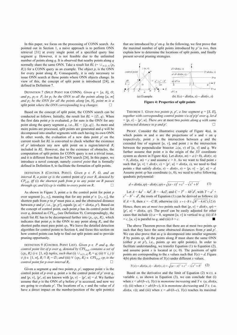
(a) Example (b) Y(x) = dist(u, s) − dist(v, s)
Figure 4: Properties of split points
THEOREM 1. Given two points p, p′, a line segment q = [S, E], together with corresponding control points v/u of p/p′ over q, let d = ||p, v|| − ||p′, u||. There are at most two points along q with same obstructed distance to p and p′. □
PROOF. Consider the illustrative example of Figure 4(a), in which points m and n are the projections of u and v on q respectively, point y is the intersection between q and the extended line of segment [u, v], and point z is the intersection between the perpendicular bisector ⊥(u, v) of [u, v] and q. We further assume that point n is the origin of the XY coordinate system as shown in Figure 4(a). Let dist(n, m) = a (> 0), dist(v, n) = b, dist(u, m) = c and assume c > b. As we want to find point s such that ||p, v|| + dist(v, s) = ||p′, u|| + dist(u, s), we need to find points s that satisfy dist(u, s) − dist(v, s) = ||p, v|| − ||p′, u|| = d. Assume point sp has coordinate (x, 0), we need to solve following quadratic polynomial:
2222)(),(),( bxcxaspvdistspudistd +−+−=−= (1)
Let A = 4a2 − 4d2, B = −4aT, and C = T2 − 4b2d2, with T = a2 + c2 − b2 − d2, the roots of Equation (1) can be derived as follows: (i) if A = 0, then x = −C/B; otherwise (ii) 2( 4 ) (2 )x B B AC A= − ± − Hence, there are at most two points such that ||p, v|| + dist(v, sp) = ||p′, u|| + dist(u, sp). The proof can be easily adjusted for other cases that include (i) a = 0, segment [u, v] is vertical to q; (ii) if b = c, [u, v] is parallel to q, and (iii) b > c. ■
The above Theorem proves that there are at most two points sp such that they have the same obstructed distances from p and p′. We can also prove that as q is decomposed into smaller segments R by points sp, all the points along R must share the same ONN (either p or p′), i.e., points sp are split point(s). In order to facilitate understanding, we transfer Equation (1) to Equation (2), and assume point s is located at (x, 0). The positions of split points are corresponding to the x values such that Y(x) = d. Figure 4(b) plots the distribution of Y(x) under different x values.
2222)(),(),()( bxcxasvdistsudistxY +−+−=−= (2)
Based on the derivative and the limit of Equation (2) w.r.t. a variable x, as shown in Equation (3), we can conclude that (i) when x < ab/(b−c), Y(x) is monotone increasing and Y ∈ (a, dist(u, v)); (ii) when x > ab/(b−c), it is monotone decreasing and Y ∈ (-a, dist(u, v)); and (iii) when x = ab/(b−c), Y(x) reaches its maximal

value2 dist(u, v). The positions of split points can be determined as follows, according to the value of d = ||p, v|| − ||p′, u|| and Y(x).
2 2
2 2
2 2 2 2
2 2
2 2
1 1 1 1
( )
( ) 0( )
1 1 01 1
( ) ( )
x ac b
x a xx a xY x x a
a x c x b
xc b
a x x
⎧− >⎪
⎪+ +⎪ −⎪
⎪ −⎪′ = − ≤ ≤⎨− + +⎪
⎪ − −⎪ − <⎪
+ +⎪− −⎪⎩
, (3)
lim ( )x
Y x a→+∞
= − , and lim ( )x
Y x a→−∞
=
Case 1: d ≥ dist(u, v). As Y(x) ≤ dist(u, v), it is for sure that for any point s along q, Y(x) = dist(u, s) − dist(v, s) ≤ d = ||p, v|| − ||p′, u||. In other words, it indicates ||p′, u|| + dist(u, s) ≤ ||p, v|| + dist(v, s), and thus new point p′ will replace p as the ONN for any point along q without introducing any new split point.
Case 2: a < d < dist(u, v). As depicted in Figure 4(b), there will be two values x1 and x2 such that Y(x1) = Y(x2) = d, with x1 < ab/(b−c) < x2. Let (x1, 0) be s1 and (x2, 0) be s2. For a given point s with coordinate (x, 0), when (i) x < x1 or x > x2, Y(x) < d which means dist(u, s) − dist(v, s) < ||p, v|| − ||p′, u||, i.e., ||p′, u|| + dist(u, s) < ||p, v|| + dist(v, s), and hence point p′ is the ONN for each point along the segments [S, s1] and [s2, E]; and (ii) x1 ≤ x ≤ x2, Y(x) ≥ d which means dist(u, s) − dist(v, s) ≥ ||p, v|| − ||p′, u||, i.e., ||p′, u|| + dist(u, s) ≥ ||p, v|| + dist(v, s), and thus point p still is the ONN for all the points along the segment [s1, s2]. In this case, p′ introduces two split points s1, s2.
Case 3: -a < d ≤ a. As depicted in Figure 4(b), there will be only one value x1 such that Y(x1) = d. Let (x1, 0) be s1. For a given point s with coordinate (x, 0), when (i) x < x1, Y(x) > d which indicates dist(u, s) − dist(v, s) > ||p, v|| − ||p′, u||, i.e., ||p′, u|| + dist(u, s) > ||p, v|| + dist(v, s), and hence point p is still the ONN for every point along the segment [S, s1]; and (ii) x ≥ x1, Y(x) ≤ d which means dist(u, s) − dist(v, s) ≤ ||p, v|| − ||p′, u||, i.e., ||p′, u|| + dist(u, s) ≤ ||p, v|| + dist(v, s), and thus point p′ is the ONN for all the points along the segment [s1, E]. In this case, p′ introduces one split point s1.
Case 4: d ≤ -a. As Y(x) > -a, it is for sure that dist(u, s) − dist(v, s) ≥ d. In other words, it indicates ||p′, u|| + dist(u, s) ≥ ||p, v|| + dist(v, s). Consequently, point p is still the ONN to any point on q.
In the above discussion, we define a quadratic polynomial whose roots can be used to derive the positions and number of split points. However, some special case of Case 1/Case 4 can be detected by Lemma 1, without any expensive calculation of the quadratic polynomial. Its pruning power will be detailed in Section 4 where we present the CONN search algorithm.
LEMMA 1. Given two points p, p′, a line segment q = [S, E], together with corresponding control points v and u, let dist⊥(cp, q)
2 Note that the distribution of Y(x) under other cases (e.g., a = 0,
b > c) has different trend, i.e., different inflexion points and maximal/minimal values.
be the vertical distance from a control point cp to a line segment q, and assume dist⊥(u, q) > dist⊥(v, q). Point p for sure is closer to any point along q compared with p′, if it satisfies (i) ||p′, u|| + dist(u, S) > ||p, v|| + dist(v, S); and (ii) ||p′, u|| + dist(u, E) > ||p, v|| + dist(v, E). □
PROOF. Without loss of generality, we assume that there is at least one point s along the segment q such that ||p′, s|| < ||p, s||. As points v and u are the control points of p and p′ over q respectively, ||p′, s|| = ||p′, u|| + dist(u, s) and ||p, s|| = ||p, v|| + dist(v, s). ||p′, s|| < ||p, s|| indicates dist(u, s) − dist(v, s) < ||p, v|| − ||p′, u|| = d. On the other hand, based on condition (i) and condition (ii), we have dist(u, S) − dist(v, S) > d and dist(u, E) − dist(v, E) > d. Let Y(t) = dist(u, t) − dist(v, t) with t ∈ [S, E]. As t varies from S to E, the value of Y(t) first drops and then increases, which contradicts the distribution of Y(t) shown in Figure 4(b). Consequently, our assumption that ||p′, s|| < ||p, s|| is invalid, and point p for sure is nearer to any point along q than p′. ■
Based on Lemma 1, we introduce a pruning distance, namely RLMAX = MAXi∈[1, t](||pi, Ri.l||, ||pi, Ri.r||)3. Given a current result list, if all the unexamined objects have their minimal distances to the query line segment larger than RLMAX, it is guaranteed that the current result list will not be changed by any unexamined object (as proved by Lemma 2). In other words, Lemma 2 provides a search termination condition which will be utilized in our CONN search algorithm that is to be presented in the next section.
LEMMA 2. Given a result list RL =∪i∈[1, t]⟨pi, cpi, Ri⟩, a point p, and a segment q = [S, E], p for sure cannot change RL if mindist(p, q) > RLMAX. □
PROOF. Without loss of generality, we assume that there is at least one point s ∈ Ri along q such that ||p, s|| < ||pi, s||. As s is a point on Ri, ||p, s|| ≥ dist(p, s) ≥ mindist(p, q). On the other hand, ||pi, s|| = ||pi, cpi|| + dist(cpi, s). Since cpi is the control point of pi over Ri ⊆ q, it is visible to any point along Ri. Consequently, dist(cpi, s) ≤ MAX(dist(cpi, Ri.l), dist(cpi, Ri.r)), i.e., ||pi, s|| ≤ ||pi, cpi|| + MAX(dist(cpi, Ri.l), dist(cpi, Ri.r)) = MAX(||pi, Ri.l||, ||pi, Ri.r||) ≤ RLMAX < mindist(p, q). Hence, ||p, s|| that is larger than mindist(p, q) for sure is larger than ||pi, s||. The assumption is invalid and the proof completes. ■
4. CONN QUERY PROCESSING In this section, we present the detailed CONN query processing
algorithm. The basic idea is to traverse the data set P in ascending order of their Euclidean distances (mindist that is the lower bound of the obstructed distance) to the query line segment q, assuming that P and O are indexed by two separate R-trees. For each data point p ∈ P visited, we first find out all the obstacles that might affect the obstructed distances from p to any point along q, then identify the control points of p over q, and finally evaluate the impact of p on the current result list RL which is initialized to ⟨∅, ∅, q⟩. In what follows, we elaborate these three steps, then propose the complete CONN search algorithm, and finally discuss the flexibility/extension of the search algorithm. To simplify the
3 If ∃ ⟨pi, cpi, Ri⟩ ∈ RL with pi = ∅, ||pi, Ri.l|| = ||pi, Ri.r|| = ∞, and
MAX(a, b) is a function to return (i) a if a ≥ b and (ii) b otherwise.

discussion, we use line segments, but not rectangles, to represent obstacles in our running examples, while the ideas can be easily extended to rectangles that are sets of line segments.
4.1 Obstacle Retrieval As mentioned in Section 1, the existing VG-based approach
needs to maintain the visibility graph and its high space and time complexities deteriorate its practicability. Actually, for a given point p and a given query line segment q = [S, E], only a small number of obstacles will affect the obstructed distances from p to any point along q. As demonstrated in Theorem 2, once the shortest path from p to S and that from p to E are identified, the search range for all the obstacles that may affect the obstructed distance between p and any point along q, denoted by SRp,q, is confirmed; and thus the obstacle retrieval can be safely terminated after all the obstacles inside SRp,q are retrieved.
S E
p
a
b
c
d
f
g
sx
o1
obstalce
qshortest path from p to S
shortest path from p to E
SRp,q
Figure 5: The obstacle search range
THEOREM 2. Given a data point p, a query segment q = [S, E],
let SRp,q be the range bounded by SP(p, S), SP(p, E), and q. ∀ s ∈ q, SP(p, s) only passes vertices of obstacles o ∈ SRp,q. □
PROOF. We assume that there is a point s ∈ q such that its shortest path SP(p, s) passes a vertex of at least one obstacle o outside SRp,q. As o ∉ SRp,q and s ∈SRp,q, SP(p, s) must intersect the boundary of SRp,q, and let point x be an intersection. Without loss of generality, we assume x is located at SP(p, S). Consequently, we have two paths from p to x, i.e., P1(p, x) following SP(p, s) and P2(p, x) following SP(p, S) but both stopping at x instead of s/S. Take Figure 5 as an example, SP(p, s) = {f, g} and SP(p, S) = {a, b}. Correspondingly, P1(p, x) = {f, g} and P2(p, x) = {a, b}. If |P1(p, x)| < |P2(p, x)|, |P1(p, x)| + ||x, S|| < |P2(p, x)| + ||x, S|| = ||p, S|| which contradicts the fact that ||p, S|| is the minimal distance between p and S. Otherwise, |P1(p, x)| ≥ |P2(p, x)|, |P1(p, x)| + ||x, s|| ≥ |P2(p, x)| + ||x, s||; and hence the path from p to s passing o1 is not the shortest path, which contradicts our assumption. Therefore, our assumption is invalid and the proof completes. ■
In order to utilize Theorem 2 to bound the search range for all the obstacles affecting the obstructed distances from p to any point along q = [S, E], both SP(p, S) and SP(p, E) have to be identified. Thus, Lemma 3 is developed.
LEMMA 3. Given a point p, a point s along q, and a path P(p, s) from p to s, suppose all the obstacles that have their minimal Euclidean distances to q bounded by |P(p, s)| have been retrieved and maintained in a set So, i.e., So = {o ∈ O | mindist(o, q) ≤ |P(p, s)|}. Let P2(p, s) be the shortest path from p to s obtained based on So. If |P2(p, s)| ≤ |P(p, s)|, it is confirmed that P2(p, s) must be the real shortest path from p to s, i.e., P2(p, s) = SP(p, s). □
PROOF. If P2(p, s) is not the real shortest path from p to s, there must be another one P3(p, s) = SP(p, s) with |P3(p, s) | < |P2(p, s)|. As P2(p, s) is the shortest one among all the paths from p to s such that they only pass the vertices of obstacles inside So, P3(p, s) must pass at least one vertex, denoted as v, of some obstacle that is not included in So, i.e., located outside the circle cir(s, |P(p, s)|) centered at s with |P(p, s)| as radius. We further decompose P3(p, s) into two paths via node v, P3(p, v) and P3(v, s). As |P3(p, s)| = |P3(p, v)| + |P3(v, s)|, |P3(p, s)| > |P3(v, s)| ≥ dist(v, s) > |P(p, s)|. On the other hand, |P2(p, s)| ≤ |P(p, s)| holds. Hence, |P3(p, s)| > |P2(p, s)| contradicts our assumption, and the proof completes. ■
Based on Theorem 2 and Lemma 3, our Incremental Obstacle Retrieval Algorithm (IOR) is developed, with its pseudo-code depicted in Algorithm 1. The basic idea is to retrieve the obstacles according to ascending order of their minimal distances to q, and add them into the local visibility graph VG which initially only includes the point p currently processed and two endpoints of q (i.e., S and E). Based on local VG, a local shortest path from p to endpoint S/E can be identified by Dijkstra’s algorithm [5], denoted as P1(p, S) and P2(p, E) (Line 2). It then fetches all the obstacles having their smallest distances to q bounded by |P1(p, S)| or |P2(p, E)|, and inserts them into local VG (Lines 6-12). Since VG is changed, both P1(p, S) and P2(p, E) need to be validated, which may trigger the retrieval of more obstacles. The process proceeds until the new P1(p, S) and P2(p, E) do not trigger the retrieval of any new obstacle. As stated in Lemma 3, P1(p, S) and P2(p, E) must represent the real shortest path from p to S/E, i.e., P1(p, S) = SP(p, S) and P2(p, E) = SP(p, E). Consequently, the range bounded by P1(p, S), P2(p, E) and q corresponds to the range SRp,q defined in Theorem 2. In other words, the fact that IOR retrieves all the obstacles with their minimal distances to q not exceeding MAX(|P1(p, S)|, |P2(p, E)|) means that all the obstacles located inside range SRp,q have been retrieved, as demonstrated in Lemma 4. Therefore, the correctness of IOR is guaranteed.
Algorithm 1 Incremental Obstacle Retrieval Algorithm (IOR) Input: obstacle R-tree To, min-heap Ho, query line segment q = [S, E], data point p, visibility graph VG, previous search distance d 1: while (1) do 2: P1(p, S) = Dijkstra(VG, p, S) and P2(p, E) = Dijkstra(VG, p, E) 3: d′ = MAX(|P1(p, S)|, |P2(p, E)|) 4: if (d′ > d) then 5: d = d′ // for the next loop 6: while Ho ≠ ∅ and Ho.head.key ≤ d do 7: de-heap the top entry (e, key) of Ho 8: if e is an obstacle then 9: add e to set So and their vertices to VG 10: else // e is a non-leaf node 11: for each child entry ei ∈ e do 12: insert (ei, mindist(ei, q)) into Ho 13: else break
LEMMA 4. Given a query line segment q = [S, E], let d =
MAX(|SP(p, S)|, |SP(p, E)|). All the obstacles that are inside range SRp,q must have their minimal distances to q bounded by d. □
PROOF. Suppose there is an obstacle o that is inside the range SRp,q with mindist(o, q) > d. Let segment l = [o, s] refer to the shortest path from o to q in an Euclidean space which intersects q at point s, i.e., mindist(o, q) = dist(o, s). Without loss of generality, we extend the segment l to l′ and assume l′ intersects SP(p, S) or
SP(p, E) at point p′, i.e., l′ = [p′, s]. Since point p′ lies along SP(p, S) or SP(p, E), ||p′, s|| ≤ MAX(|SP(p, S)|, |SP(p, E)|) = d. On the other hand, dist(o, s) ≤ dist(p′, s) ≤ ||p′, s|| ≤ d. Consequently, our assumption that mindist(o, q) = dist(o, s) > d is not valid. The proof completes. ■
In addition, we would like to highlight that the local visibility graph VG formed by a point p can be reused by a point p′ that is accessed/evaluated after p. If p′ does not trigger the retrieval of any new obstacle (i.e., current VG has already covered the search range SRp′,q), IOR for point p′ can be safely terminated by reusing the current VG. Otherwise, it expands the local VG by adding new obstacles until the search range SRp′,q has been fully covered. Therefore, the IOR for all the points in P will access the obstacle set O at most once.
4.2 Control Point List Computation Once the local VG contains all the obstacles that may affect the
obstructed distances from a specified data point p to q, our next step is to find out the control point list of p over q, i.e., CPLp,q. A straightforward approach is to utilize the fact that a control point over R must be visible to R and invoke Dijkstra’s algorithm to form the shortest path from p to every node n that is within the SRp,q
4. For each n ∈ SRp,q, we get the visible region VRn,q, and add a new tuple ⟨n, Rn = VRn,q⟩ to CPLp,q, assuming that n is the control point of p over VRn,q. If Rn overlaps Rm that is associated with some other control point m included in current CPLp,q (i.e., ∃ ⟨m, Rm⟩ ∈ CPLp,q with Rn ∩ Rm ≠ ∅), an update is performed. Obviously, this method is expensive, especially when the number of nodes inside SRp,q is large. In order to handle this issue and improve the performance, we propose several Lemmas that can simplify the evaluation cost of some nodes n ∈ SRp,q.
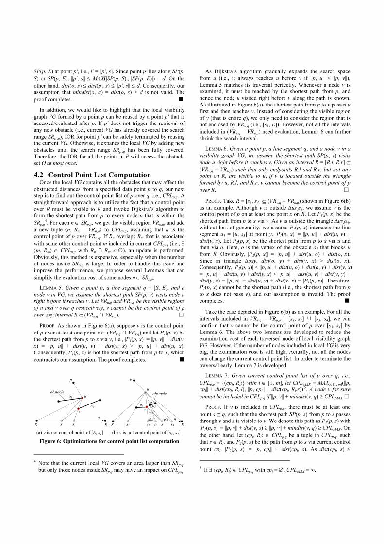
LEMMA 5. Given a point p, a line segment q = [S, E], and a node v in VG, we assume the shortest path SP(p, v) visits node u right before it reaches v. Let VRu,q and VRv,q be the visible regions of u and v over q respectively, v cannot be the control point of p over any interval R ⊆ (VRu,q ∩ VRv,q). □
PROOF. As shown in Figure 6(a), suppose v is the control point of p over at least one point x ∈ (VRu,q ∩ VRv,q) and let P1(p, x) be the shortest path from p to x via v, i.e., |P1(p, x)| = ||p, v|| + dist(v, x) = ||p, u|| + dist(u, v) + dist(v, x) > ||p, u|| + dist(u, x). Consequently, P1(p, x) is not the shortest path from p to x, which contradicts our assumption. The proof completes. ■
S Es1x
u
v
p
q
o1
o2
obstacle
S Es2s1
qx s4s3
o1 o2
obstacle
yv
u
p
R.l R.r
o
(a) v is not control point of [S, s1] (b) v is not control point of [s3, s4]
Figure 6: Optimizations for control point list computation
4 Note that the current local VG covers an area larger than SRp,q,
but only those nodes inside SRp,q may have an impact on CPLp,q.
As Dijkstra’s algorithm gradually expands the search space from q (i.e., it always reaches u before v if ||p, u|| < ||p, v||), Lemma 5 matches its traversal perfectly. Whenever a node v is examined, it must be reached by the shortest path from p, and hence the node u visited right before v along the path is known. As illustrated in Figure 6(a), the shortest path from p to v passes u first and then reaches v. Instead of considering the visible region of v (that is entire q), we only need to consider the region that is not enclosed by VRu,q (i.e., [s1, E]). However, not all the intervals included in (VRv,q − VRu,q) need evaluation, Lemma 6 can further shrink the search interval.
LEMMA 6. Given a point p, a line segment q, and a node v in a visibility graph VG, we assume the shortest path SP(p, v) visits node u right before it reaches v. Given an interval R = [R.l, R.r] ⊆ (VRv,q − VRu,q) such that only endpoints R.l and R.r, but not any point on R, are visible to u, if v is located outside the triangle formed by u, R.l, and R.r, v cannot become the control point of p over R. □
PROOF. Take R = [s3, s4] ⊆ (VRv,q − VRu,q) shown in Figure 6(b) as an example. Although v is outside ∆us3s4, we assume v is the control point of p on at least one point x on R. Let P1(p, x) be the shortest path from p to x via v. As v is outside the triangle ∆us3s4, without loss of generality, we assume P1(p, x) intersects the line segment q1 = [u, s3] at point y. |P1(p, x)| = ||p, u|| + dist(u, v) + dist(v, x). Let P2(p, x) be the shortest path from p to x via u and then via o. Here, o is the vertex of the obstacle o2 that blocks u from R. Obviously, |P2(p, x)| = ||p, u|| + dist(u, o) + dist(o, x). Since in triangle ∆oxy, dist(o, y) + dist(y, x) > dist(o, x). Consequently, |P2(p, x)| < ||p, u|| + dist(u, o) + dist(o, y) + dist(y, x) = ||p, u|| + dist(u, y) + dist(y, x) < ||p, u|| + dist(u, v) + dist(v, y) + dist(y, x) = ||p, u|| + dist(u, v) + dist(v, x) = |P1(p, x)|. Therefore, P1(p, x) cannot be the shortest path (i.e., the shortest path from p to x does not pass v), and our assumption is invalid. The proof completes. ■
Take the case depicted in Figure 6(b) as an example. For all the intervals included in VRv,q − VRu,q = [s1, s2] ∪ [s3, s4], we can confirm that v cannot be the control point of p over [s3, s4] by Lemma 6. The above two lemmas are developed to reduce the examination cost of each traversed node of local visibility graph VG. However, if the number of nodes included in local VG is very big, the examination cost is still high. Actually, not all the nodes can change the current control point list. In order to terminate the traversal early, Lemma 7 is developed.
LEMMA 7. Given current control point list of p over q, i.e., CPLp,q = {⟨cpi, Ri⟩} with i ∈ [1, m], let CPLMAX = MAXi∈[1, m](||p, cpi|| + dist(cpi, Ri.l), ||p, cpi|| + dist(cpi, Ri.r)) 5. A node v for sure cannot be included in CPLp,q if ||p, v|| + mindist(v, q) ≥ CPLMAX.□
PROOF. If v is included in CPLp,q, there must be at least one point s ⊆ q, such that the shortest path SP(p, s) from p to s passes through v and s is visible to v. We denote this path as P1(p, s) with |P1(p, s)| = ||p, v|| + dist(v, s) ≥ ||p, v|| + mindist(v, q) ≥ CPLMAX. On the other hand, let ⟨cpi, Ri⟩ ∈ CPLp,q be a tuple in CPLp,q, such that s ∈ Ri, and P2(p, s) be the path from p to s via current control point cpi. |P2(p, s)| = ||p, cpi|| + dist(cpi, s). As dist(cpi, s) ≤
5 If ∃ ⟨cpi, Ri⟩ ∈ CPLp,q with cpi = ∅, CPLMAX = ∞.
MAX(dist(cpi, Ri.l), dist(cpi, Ri.r)), |P2(p, s)| ≤ CPLMAX ≤ |P1(p, s)|, and thus P1(p, s) cannot be the shortest path from p to s. The proof completes. ■
Lemma 7 serves as the termination condition of Control Point List Computation Algorithm (CPLC) that is shown in Algorithm 2. CPLC shares the basic idea as the approach we mentioned earlier. That is to call Dijkstra’s algorithm to gradually traverse the local visibility graph VG and to access nodes v according to ascending order of their obstructed distances to p. The p’s control point list CPLp,q over q is updated during the traversal. However, different from the straightforward method, it employs Lemma 5 and Lemma 6 to significantly reduce the node examination cost. The Split function invoked (Line 14) is the same as the split point computation algorithm presented in Section 3. Before v is considered, all the shortest paths from p to any point along Rint pass the control point cpi, and now we want to check whether the path from p to any point along Rint via v is even shorter. Algorithm 2 Control Point List Computation Algorithm (CPLC) Input: query line segment q = [S, E], data point p, visibility graph VG Output: p’s control point list CPLp,q over q 1: CPLp,q = {⟨∅, [S, E]⟩} 2: while there exists a node in VG that has not been visited do 3: let v ∈ VG be the one with the smallest obstructed distance to p among those nodes not yet visited 4: if ||p, v|| ≥ CPLMAX then // Lemma 7 5: break 6: let u be the node that SP(p, v) passes right before reaching v 7: R = VRv − VRu // Lemma 5 8: refine R based on Lemma 6 9: for each tuple ⟨cpi, Ri⟩ in CPLp,q do // update CPLp,q 10: Rint = R ∩ Ri 11: if Rint ≠ ∅ and cpi = ∅ then 12: replace ⟨cpi, Ri⟩ with ⟨v, Rint ⟩ and ⟨cpi, Ri − Rint ⟩ 13: else if Rint ≠ ∅ and cpi ≠ ∅ then 14: d = ||p, cpi|| − ||p, v|| and Split(p, cpi, p, v, Rint, d) 15: return CPLp,q
There are four cases, as discussed in Section 3, with d = ||p, cpi|| − ||p, v|| and a as the difference between v’s projection on q and cpi’s projection on q: (i) Case 1: d ≥ dist(cpi, v), ⟨cpi, Ri⟩ is replaced with ⟨v, Rint⟩ (Rint = R ∩ Ri) and ⟨cpi, Ri − Rint⟩. (ii) Case 2: a < d < dist(cpi, v), interval Rint will be decomposed into three segments by points x1 and x2, with x1 and x2 derived based on Equation (1). Thereafter, ⟨cpi, Ri⟩ is replaced accordingly. (iii) Case 3: -a < d ≤ a, Rint will be decomposed into two segments by point x1 with x1 derived based on Equation (1) too. Again, ⟨cpi, Ri⟩ is replaced accordingly. (iv) Case 4: d ≤ -a, ⟨cpi, Ri⟩ remains. The process proceeds until all the nodes in local VG are traversed or the visited node satisfies ||p, v|| ≥ CPLMAX. As nodes in local VG are traversed based on ascending order of their obstructed distances to p, when currently visited node has its obstructed distance to p larger than CPLMAX, all the remaining nodes n in VG must satisfy ||p, n|| ≥ CPLMAX. Note that the termination condition relaxes Lemma 7 using zero as the lower bound of mindist(n, q).
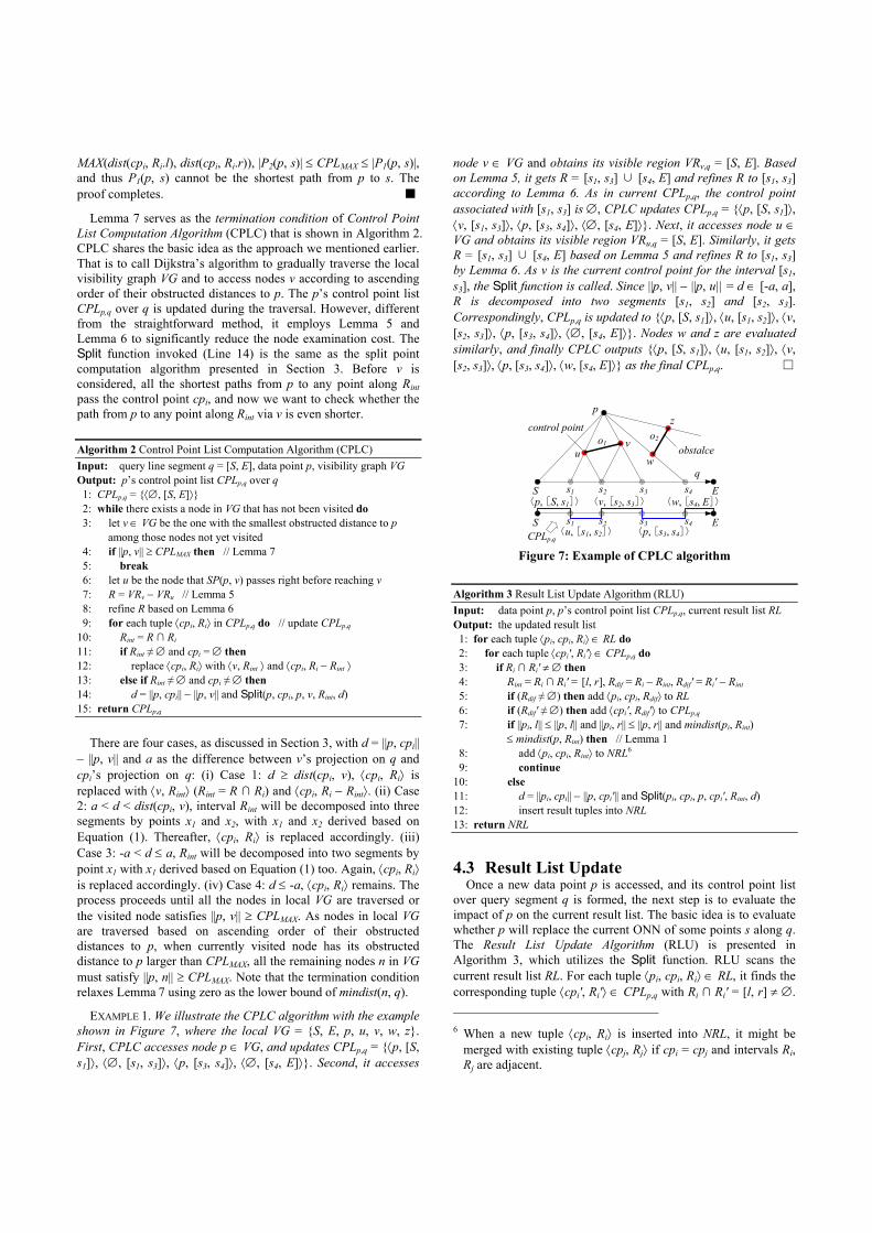
EXAMPLE 1. We illustrate the CPLC algorithm with the example shown in Figure 7, where the local VG = {S, E, p, u, v, w, z}. First, CPLC accesses node p ∈ VG, and updates CPLp,q = {⟨p, [S, s1]⟩, ⟨∅, [s1, s3]⟩, ⟨p, [s3, s4]⟩, ⟨∅, [s4, E]⟩}. Second, it accesses
node v ∈ VG and obtains its visible region VRv,q = [S, E]. Based on Lemma 5, it gets R = [s1, s3] ∪ [s4, E] and refines R to [s1, s3] according to Lemma 6. As in current CPLp,q, the control point associated with [s1, s3] is ∅, CPLC updates CPLp,q = {⟨p, [S, s1]⟩, ⟨v, [s1, s3]⟩, ⟨p, [s3, s4]⟩, ⟨∅, [s4, E]⟩}. Next, it accesses node u ∈ VG and obtains its visible region VRu,q = [S, E]. Similarly, it gets R = [s1, s3] ∪ [s4, E] based on Lemma 5 and refines R to [s1, s3] by Lemma 6. As v is the current control point for the interval [s1, s3], the Split function is called. Since ||p, v|| − ||p, u|| = d ∈ [-a, a], R is decomposed into two segments [s1, s2] and [s2, s3]. Correspondingly, CPLp,q is updated to {⟨p, [S, s1]⟩, ⟨u, [s1, s2]⟩, ⟨v, [s2, s3]⟩, ⟨p, [s3, s4]⟩, ⟨∅, [s4, E]⟩}. Nodes w and z are evaluated similarly, and finally CPLC outputs {⟨p, [S, s1]⟩, ⟨u, [s1, s2]⟩, ⟨v, [s2, s3]⟩, ⟨p, [s3, s4]⟩, ⟨w, [s4, E]⟩} as the final CPLp,q. □
S Es1 s2 s3 s4
S Es1 s2 s3 s4
p
o1
q
〈p, [S, s1]〉
o2
uv
w
z
obstalce
〈u, [s1, s2]〉CPLp,q
〈v, [s2, s3]〉
〈p, [s3, s4]〉
〈w, [s4, E]〉
control point
Figure 7: Example of CPLC algorithm
Algorithm 3 Result List Update Algorithm (RLU) Input: data point p, p’s control point list CPLp,q, current result list RL Output: the updated result list 1: for each tuple ⟨pi, cpi, Ri⟩ ∈ RL do 2: for each tuple ⟨cpi′, Ri′⟩ ∈ CPLp,q do 3: if Ri ∩ Ri′ ≠ ∅ then 4: Rint = Ri ∩ Ri′ = [l, r], Rdif = Ri − Rint, Rdif′ = Ri′ − Rint 5: if (Rdif ≠ ∅) then add ⟨pi, cpi, Rdif⟩ to RL 6: if (Rdif′ ≠ ∅) then add ⟨cpi′, Rdif′⟩ to CPLp,q 7: if ||pi, l|| ≤ ||p, l|| and ||pi, r|| ≤ ||p, r|| and mindist(pi, Rint) ≤ mindist(p, Rint) then // Lemma 1 8: add ⟨pi, cpi, Rint⟩ to NRL6 9: continue 10: else 11: d = ||pi, cpi|| − ||p, cpi′|| and Split(pi, cpi, p, cpi′, Rint, d) 12: insert result tuples into NRL 13: return NRL
4.3 Result List Update Once a new data point p is accessed, and its control point list
over query segment q is formed, the next step is to evaluate the impact of p on the current result list. The basic idea is to evaluate whether p will replace the current ONN of some points s along q. The Result List Update Algorithm (RLU) is presented in Algorithm 3, which utilizes the Split function. RLU scans the current result list RL. For each tuple ⟨pi, cpi, Ri⟩ ∈ RL, it finds the corresponding tuple ⟨cpi′, Ri′⟩ ∈ CPLp,q with Ri ∩ Ri′ = [l, r] ≠ ∅. 6 When a new tuple ⟨cpi, Ri⟩ is inserted into NRL, it might be
merged with existing tuple ⟨cpj, Rj⟩ if cpi = cpj and intervals Ri, Rj are adjacent.
By solving the Equation (1) (i.e., dist(cpi, x) – dist(cpi′, x) = ||pi, cpi|| − ||p, cpi′|| with x ∈ [l, r]), it can update the result list accordingly. As the details of split point calculation algorithm (i.e., Split) have been already presented in Section 3, we use a running example to illustrate the RLU algorithm.
qS Es1
o1
o3
o2a
b
c
s2 s3 s4 s5
obstalce
v1
v2
v5
v6
v3
v4
Figure 8: Example of RLU algorithm
EXAMPLE 2. As shown in Figure 8, P = {a, b, c}, O = {o1, o2,
o3}, and q = [S, E]. Suppose that point a has been processed, with current RL = {⟨a, a, [S, s3]⟩, ⟨a, v1, [s3, s5]⟩, ⟨a, v2, [s5, E]⟩} and data point b is going to be evaluated with its control point list CPLb,q = {⟨b, [S, s2]⟩, ⟨v5, [s2, s4]⟩, ⟨v6, [s4, E]⟩}. Now we invoke RLU to evaluate the impact of b on RL. First, the tuple ⟨a, a, [S, s3]⟩ ∈ RL is compared with ⟨b, [S, s2]⟩ ∈ CPLb,q. Based on the Split function, Rint (= [S, s3] ∩ [S, s2] = [S, s2]) is partitioned into two segments (i.e., Case 3), and NRL = {⟨a, a, [S, s1]⟩, ⟨b, b, [s1, s2]⟩}. Next, the tuple ⟨a, a, [s2, s3]⟩ ∈ RL is compared with ⟨v5, [s2, s4]⟩ ∈ CPLb,q. Again, based on the Split function, the entire Rint (= [s2, s3] ∩ [s2, s4] = [s2, s3]) is closer to b than to a, and thus NRL = {⟨a, a, [S, s1]⟩, ⟨b, b, [s1, s2]⟩, ⟨b, v5, [s2, s3]⟩}. Then, the tuple ⟨a, v1, [s3, s5]⟩ ∈ RL is compared with ⟨v5, [s3, s4]⟩∈ CPLb,q. Similarly, Split function detects that Rint (= [s3, s5] ∩ [s3, s4] = [s3, s4]) is closer to b than to a, and hence NRL is updated to {⟨a, a, [S, s1]⟩, ⟨b, b, [s1, s2]⟩, ⟨b, v5, [s2, s4]⟩}. The process proceeds until all the tuples in RL are evaluated, and the final NRL = {⟨a, a, [S, s1]⟩, ⟨b, b, [s1, s2]⟩, ⟨b, v5, [s2, s4]⟩, ⟨b, v6, [s4, E]⟩}. □
Algorithm 4 CONN Search Algorithm (CONN) Input: data R-tree Tp, obstacle R-tree To, query line segment q = [S, E] Output: result list RL of the CONN query 1: RL = {⟨∅, ∅, [S, E]⟩}, RLMAX = ∞, VG = {S, E}, d = 0 2: a min-heap Hp = (root(Tp), 0), a min-heap Ho = (root(To), 0) 3: while Hp ≠ ∅ and Hp.head.key < RLMAX do // Lemma 2 4: de-heap the top entry (e, key) of Hp 5: if e is a data point then 6: insert e into local visibility graph VG 7: IOR (To, Ho, q, e, VG, d) // see Algorithm 1 8: CPLe,q = CPLC (q, e, VG) // see Algorithm 2 9: remove e from VG 10: RL = RLU (e, CPLe,q, RL) // see Algorithm 3 11: else // e is an intermediate (i.e., non-leaf) node 12: for each child entry ei ∈ e do 13: insert (ei, mindist(ei, q)) into Hp 14: return RL
4.4 CONN Search Algorithm Our CONN Search Algorithm (CONN) traverses the data set P
in ascending order of their minimal Euclidean distances to q (i.e.,
mindist). For each accessed data point p ∈ P, it invokes IOR to retrieve all the obstacles that might affect the obstructed distances from p to any point along q, calls CPLC to get the control point list CPLp,q of p over q, and updates the result list via RLU. The process proceeds until all the data points in P are evaluated or the termination condition is satisfied, that is mindist(p, q) > RLMAX (Lemma 2). Algorithm 4 presents the pseudo-code of CONN.
It is observed that the CONN algorithm traverses the data R-tree Tp and the obstacle R-tree To at most once. Let |Tp| and |To| be the tree size of Tp and To respectively, |VG| be the number of nodes in VG, |R| be the maximal number of tuples included in RL, CPLp,q (∀ p ∈ P), and VRn,q (∀ n ∈ VG), and N be the number of data points accessed during the CONN search. The time complexity and the correctness of CONN algorithm are analyzed as follows.
THEOREM 3. The time complexity of the CONN algorithm is O (N × log |Tp| × log |To| × |VG| × log |VG|). □
PROOF. For every data point p ∈ P visited during the search, the CONN algorithm takes O (|VG| × log |VG|) to insert p into VG, takes O (log |To| × |VG| × log |VG|) for IOR, takes O (|VG| × log |VG| × |R|2) for CPLC, takes O (|R|2) for RLU, and incurs O (|VG| × log |VG|) to delete p from VG. Consequently, the time complexity of the CONN algorithm is O (N × log |Tp| × (|VG| × log |VG| + log |To| × |VG| × log |VG| + |VG| × log |VG| × |R|2 + |R|2 + |VG| × log |VG|)) ≈ O (N × log |Tp| × log |To| × |VG| × log |VG|) as |VG| << |To| (as demonstrated by our experimental results to be presented in Section 5) and |R| << |Tp|. ■
THEOREM 4. The CONN algorithm retrieves exactly the ONN of every point along a given query line segment, i.e., the algorithm has no false misses and no false hits. □
4.5 Discussion Our previously proposed CONN algorithm assumes the data set
P and the obstacle set O are indexed by two different R-trees. However, it can be naturally extended to perform CONN search when P and O are indexed by a single R-tree. The detailed extensions are listed as follows: (i) It requires only one heap H to store the candidate entries (including data points, obstacles, and nodes), sorted in ascending order of their minimum distances to the specified query line segment q. (ii) When processing the top entry e de-heaped from H, it distinguishes three cases: (1) e is an obstacle. It inserts e into VG. (2) e is a data point. It calls the IOR to retrieve all the obstacles that may affect the obstructed distance from e to any point on q, gets e’s control point list CPLe,q over q via CPLC, and finally updates the result list RL via RLU. It is worth noting that during the obstacle retrieval via IOR, it is possible to access some data points which will be en-heaped into H for later processing. (3) e is an intermediate node, its child entries are en-heaped to H for later evaluation.
In addition, our proposed CONN query processing approaches can be easily extended to tackle continuous obstructed k-nearest neighbor (COkNN) search, which finds the k (≥ 1) obstructed nearest neighbors (ONNs) to every point along a specified query line segment. Due to the space limitation, we only list the major differences. First, the output of a COkNN query contains a set of ⟨ONNSi, Ri⟩ tuples, where ONNSi is the set of ONNs for each point on the interval Ri (= [Ri.l, Ri.r]) ⊆ q. Second, the pruning
distance RLMAX used in Lemma 2 has to be updated to MAXi∈[1, t] (maxodist(ONNSi, Ri.l), maxodist(ONNSi, Ri.r)), in which maxodist(ONNS, s) represents the maximal obstructed distance from any point in set ONNS to point s, i.e., MAXp∈ONNS(||p, s||).
5. EXPERIMENTAL EVALUATION This section evaluates the performance of the proposed
algorithms. We first describe experimental settings, and then present experimental results and our findings. All the algorithms were implemented in C++ and the experiments were conducted on an Intel Core 2 Duo 2.33 GHz PC with 3.25GB RAM.
5.1 Experimental Setup Our experiments are based on both real and synthetic datasets,
with the search space fixed at a [0, 10000] × [0, 10000] square shaped range. Two real datasets are deployed, namely CA and LA7. CA contains 2D points, representing 60,344 locations in California; and LA includes 2D rectangles, representing 131,461 MBRs of streets in Los Angeles. All datasets are normalized in order to fit the search range. Synthetic datasets are generated based on uniform distribution and zipf distribution, with the cardinality varying from 0.1×|LA| to 10×|LA|. The coordinate of each point in Uniform datasets is generated uniformly along each dimension, and that of each point in Zipf datasets is generated according to zipf distribution with skew coefficient α = 0.8. We assume a point’s coordinates on both dimensions are mutually independent. As COkNN (k ≥ 1) search involves a data set P and an obstacle set O, we deploy three different combinations of the datasets, namely CL, UL, and ZL, representing (P, O) = (CA, LA), (Uniform, LA), and (Zipf, LA), respectively. Note that the data points in P are allowed to lie on the boundaries of the obstacles but not in their interiors.
All data and obstacle sets are indexed by an R*-tree [1], with the page size fixed at 4KB. The performance metrics in our performance study include I/O cost (i.e., number of pages accessed), CPU time, query cost (i.e., the sum of the I/O time and CPU time, where the I/O time is computed by charging 10ms for each page fault), visibility graph size |SVG| (i.e., number of vertices in visibility graph), number of points evaluated (NPE) during search, and number of obstacles evaluated (NOE) during search. Unless specifically stated, the size of LRU buffer is 0 in the experiments, i.e., the I/O cost is determined by the number of nodes accessed. We investigate the efficiency and effectiveness of our proposed algorithms under various parameters, which are summarized in Table 2. The numbers in bold represent default settings. In each experiment, we evaluate the impact of one parameter while others are fixed at their default values, and run 100 COkNN queries with their average performance reported. The starting point and the orientation (in [0, 2π)) of the query line segment are randomly generated, while its length is controlled by the parameter ql.
Table 2. Parameter ranges and default values Parameter Range query length ql (% of data space side) 1.5, 3, 4.5, 6, 7.5 k 1, 3, 5, 7, 9 |P|/|O| 0.1, 0.2, 0.5, 1, 2, 5, 10 buffer size bs (% of the tree size) 0, 1, 2, 4, 8, 16, 32
7 CA and LA are available in the site: http://www.rtreepo rtal.org.
5.2 Performance Study The first set of experiments studies the effect of query length ql
(% of data space side). Figure 9 shows the efficiency of the COkNN algorithm as a function of ql, by fixing k = 5. It is observed that the total query time (breaking into I/O and CPU cost), NPE, and NOE grow with ql. The reason behind is that, as the query segment becomes longer, the number of candidate data points processed, the number of obstacles encountered, and the number of split points generated increase, which results in more distance computation, more control point list computation, and more result list update. Figure 9(b) illustrates the size of visibility graph (i.e., |SVG|) with respect to ql. As all the obstacles are in rectangular shapes, there are 4 × |O| = 525,844 vertexes in a global visibility graph when O = LA, denoted as FULL in Figure 9(b). Notice that although |SVG| ascends with the growth of ql, its size is much smaller than the size of FULL, as also demonstrated in the subsequent experimental results. This further demonstrates the effectiveness of our proposed incremental obstacle retrieval (IOR) algorithm in reducing the number of obstacle traversals.
1e-1
1e+0
1e+1
1e+2
1e+3
1e+4
1.5 3 4.5 6 7.5query length (% of data space side)
tota
l tim
e (s
ec)
1e+0
1e+1
1e+2
1e+3
1e+4
num
ber o
f ite
ms e
valu
atedI/O
CPUNPENOE
1e+01e+1
1e+21e+3
1e+41e+5
1e+6
1.5 3 4.5 6 7.5query length (% of data space side)
visi
bilit
y gr
aph
size |SVG|
Full
137693
16513655 6368
actual number of vertices in visibility graph
(a) CL (k = 5) (b) CL (k = 5)
Figure 9: Performance vs. ql (% of data space side) Figure 10 depicts the performance of the COkNN algorithm
with respect to k, with ql fixed at 4.5%. As expected, all costs involving total query time, NPE, NOE, and |SVG| increase with k. This is because a larger value of k implies a larger search range (for both data points and obstacles) and hence more distance computations are incurred. Furthermore, as k grows, the number of answer points in the final result list increases, which results in more frequent update operations and thus more expensive maintenance cost of the result list.
1e-1
1e+0
1e+1
1e+2
1e+3
1 3 5 7 9k
tota
l tim
e (s
ec)
0
100
200
300
400
500
num
ber o
f ite
ms e
valu
ated
I/O CPU
NPENOE
1e+0
1e+1
1e+2
1e+3
1e+4
1e+5
1e+6
1 3 5 7 9k
visi
bilit
y gr
aph
size |SVG|
Full
1545 1615 1651 1701 1740
(a) CL (ql = 4.5%) (b) CL (ql = 4.5%)
Figure 10: Performance vs. k Figure 11 plots the efficiency of the COkNN algorithm as a
function of the ratio of the cardinality of the data set P to that of the obstacle set O, i.e., |P|/|O|, with k = 5 and ql = 4.5%. A crucial observation is that the cost of the COkNN algorithm first drops and then increases as |P|/|O| varies from 0.1 to 10. In particular, the query time of COkNN decreases when |P|/|O| increases (e.g.,

from 0.1 to 0.5 in Figure 11(c)). This is because, as the density of data set P grows, the search space of COkNN becomes smaller. Accordingly, the number of obstacles that might affect the obstructed distances from data points to any point on a given query line segment is decreased (i.e., the IOR algorithm retrieves less obstacles), which is indicated by NOE in Figures 11(a) and 11(c). However, as |P|/|O| continues ascending (e.g., from 1 to 10 in Figure 11(c)), the cost of COkNN gradually increases. This is because the interval dominated by each data point becomes shorter, and the result list contains more answer points. In other words, more candidate data points need evaluation as implied by NPE in Figures 11(a) and 11(c), which in turn increases the split point computation overhead and the result list update cost. Observe that when P and O share similar cardinalities (e.g., |P|/|O| = 0.5), COkNN incurs the shortest query time. Since the search space of COkNN decreases as |P|/|O| increases, |SVG| drops with |P|/|O| as shown in Figures 11(b) and 11(d).
1e-1
1e+0
1e+1
1e+2
0.1 0.2 0.5 1 2 5 10|P|/|O|
tota
l tim
e (s
ec)
050100150200250300
num
ber o
f ite
ms e
valu
atedI/O
CPUNPENOE
1e+0
1e+1
1e+2
1e+3
1e+4
1e+5
1e+6
0.1 0.2 0.5 1 2 5 10|P|/|O|
visi
bilit
y gr
aph
size |SVG|
Full957 818 670 603 598 553 541
(a) UL (k = 5, ql = 4.5%) (b) UL (k = 5, ql = 4.5%)
0
0.7
1.4
2.1
2.8
3.5
0.1 0.2 0.5 1 2 5 10|P|/|O|
tota
l tim
e (s
ec)
0
90
180
270
360
450
num
ber o
f ite
ms e
valu
atedI/O
CPUNPENOE
1e+0
1e+11e+2
1e+3
1e+41e+5
1e+6
0.1 0.2 0.5 1 2 5 10|P|/|O|
visi
bilit
y gr
aph
size |SVG|
Full
218 185 144 137 135 133 131
(c) ZL (k = 5, ql = 4.5%) (d) ZL (k = 5, ql = 4.5%)
Figure 11: Performance vs. |P|/|O| All the previous experiments are conducted without any buffer
(i.e., the size of LRU buffer is 0). In this set of experiments, we examine the influence of buffer size bs on the COkNN search performance, with bs varying from 1% to 32% of each R-tree size. The results are plotted in Figure 12, by fixing k = 5 and ql = 4.5%. To obtain stable statistics, we use the first 50 queries to warm up the buffer and only report the average performance of the last 50 queries. It is observed that non-zero buffer can only improve I/O performance, but not others.
1e-1
1e+0
1e+1
1e+2
1 2 4 8 16 32buffer size (% of the tree size)
tota
l tim
e (s
ec)
0
90
180
270
360
450
num
ber o
f ite
ms e
valu
ated
I/O CPU NPE NOE
1e+0
1e+1
1e+2
1e+3
1e+4
1e+5
1e+6
1 2 4 8 16 32buffer size (% of the tree size)
visi
bilit
y gr
aph
size |SVG|
Full
1651 1651 1651 1651 1651 1651
(a) CL (k = 5, ql = 4.5%) (b) CL (k = 5, ql = 4.5%)
1e-1
1e+0
1e+1
1e+2
1 2 4 8 16 32buffer size (% of the tree size)
tota
l tim
e (s
ec)
0
50
100
150
200
250
num
ber o
f ite
ms e
valu
ated
I/O CPU NPE NOE
1e+0
1e+11e+2
1e+3
1e+41e+5
1e+6
1 2 4 8 16 32buffer size (% of the tree size)
visi
bilit
y gr
aph
size |SVG|
Full
876 876 876 876 876 876
(c) UL (k = 5, ql = 4.5%) (d) UL (k = 5, ql = 4.5%)
Figure 12: Performance vs. bs (% of the tree size) In all the above experiments, we assume data set P and obstacle
set O are indexed by two separate R-trees. However, as mentioned in Section 4.5, our proposed CONN search algorithm is very flexible, and it can support the case where both P and O are indexed by a single R-tree. In the last set of experiments, we compare the performance of COkNN retrieval when P and O are indexed by two different R-trees (denoted as 2T) against that under the scenario where they are indexed by one unified R-tree (denoted as 1T), and the experimental results are shown in Figure 13. It shows that 1T is more efficient than 2T in most cases. This is because when both data points and obstacles are indexed by one R-tree, only one traversal of the unified R-tree is required. Data points and obstacles that are close to each other could be found in the same leaf node of the R-tree. Based on this result, when we perform expensive spatial data mining tasks, it is more beneficial to build a single R-tree for both data points and obstacles.
1e-1
1e+0
1e+1
1e+2
1e+3
1e+4
1.5 3 4.5 6 7.5query length (% of data space side)
tota
l tim
e (s
ec)
COkNN-1TCOkNN-2T
1e-1
1e+0
1e+1
1e+2
1e+3
1e+4
1.5 3 4.5 6 7.5query length (% of data space side)
tota
l tim
e (s
ec)
COkNN-1TCOkNN-2T
(a) CL (k = 5) (b) UL (k = 5)
60
70
80
90
100
110
1 3 5 7 9k
tota
l tim
e (s
ec)
COkNN-1TCOkNN-2T
0
7
14
21
28
35
1 3 5 7 9k
tota
l tim
e (s
ec)
COkNN-1TCOkNN-2T
(c) CL (ql = 4.5%) (d) UL (ql = 4.5%)
0
7
14
21
28
35
0.1 0.2 0.5 1 2 5 10|P|/|O|
tota
l tim
e (s
ec)
COkNN-1TCOkNN-2T
0
2
4
6
8
10
0.1 0.2 0.5 1 2 5 10|P|/|O|
tota
l tim
e (s
ec)
COkNN-1TCOkNN-2T
(e) UL (k = 5, ql = 4.5%) (f) ZL (k = 5, ql = 4.5%)
Figure 13: COkNN on two R-trees vs. its on one R-tree
6. CONCLUSIONS In this paper, for the first time, we identify and solve a novel
type of CNN queries, namely continuous obstructed nearest neighbor (CONN) search, which considers the impact of obstacles on the distances between objects. CONN queries are not only interesting from a research point of view, but also useful in many applications such as location-based services, geographic information systems, and spatial data analysis. We carry out a systematic study of CONN retrieval. First, we provide a formal definition of the problem. Then, we present several effective pruning strategies and develop efficient algorithms for CONN query processing. Next, we extend our techniques to handle COkNN search, a natural generalization of CONN query. Finally, we conduct extensive experiments to verify the efficiency and effectiveness of our proposed algorithms using both real and synthetic datasets.
This work also motivates several directions for future research. We plan to extend our methods to other CONN query variations such as trajectory CONN which aims at retrieving the ONN of every point on a specified moving trajectory that consists of several consecutive line segments, and it would be also interesting to investigate CONN queries for moving objects. In addition, it is a challenging yet exciting topic to explore other forms of spatial queries with obstacle constraints (e.g., obstructed reverse nearest neighbor search, etc.).
7. REFERENCES [1] N. Beckmann, H.-P. Kriegel, R. Schneider, and B. Seeger.
The R*-tree: An efficient and robust access method for points and rectangles. In SIGMOD, pages 322–331, 1990.
[2] M. de Berg, M. van Kreveld, M. Overmars, and O. Schwarzkopf. Computational Geometry: Algorithms and Applications, Second Edition. Springer-Verlag, 2000.
[3] K. L. Cheung and A. W-C Fu. Enhanced nearest neighbour search on the R-tree. SIGMOD Record, 27(3):16–21, 1998.
[4] H.-J. Cho and C.-W. Chung. An efficient and scalable approach to CNN queries in a road network. In VLDB, pages 865–876, 2005.
[5] E. Dijkstra. A note on two problems in connexion with graphs. Numerische Mathematik, 1:269–271, 1959.
[6] V. Estivill-Castro and I. Lee. Autoclust+: Automatic clustering of point-data sets in the presence of obstacles. In TSDM, pages 133–146, 2000.
[7] J. Feng and T. Watanabe. A fast method for continuous nearest target objects query on road network. In VSMM, pages 182–191, 2002.
[8] Y. Gao, B. Zheng, G. Chen, W.-C. Lee, Ken C. K. Lee, and Q. Li. Visible reverse nearest neighbor queries. In ICDE, pages 1203–1206, 2009.
[9] Y. Gao, B. Zheng, W.-C. Lee, and G. Chen. Continuous visible nearest neighbor queries. In EDBT, pages 144–155, 2009.
[10] S. K. Ghosh and D. M. Mount. An output sensitive algorithm for computing visibility graphs. In FOCS, pages 11–19, 1987.
[11] A. Guttman. R-trees: A dynamic index structure for spatial searching. In SIGMOD, pages 47–57, 1984.
[12] A. Henrich. A distance-scan algorithm for spatial access structures. In GIS, pages 136–143, 1994.
[13] G. R. Hjaltason and H. Samet. Distance browsing in spatial databases. ACM Transactions on Database Systems, 24(2):265–318, 1999.
[14] M. R. Kolahdouzan and C. Shahabi. Alternative solutions for continuous k nearest neighbor queries in spatial network databases. GeoInformatica, 9(4):321–341, 2005.
[15] S. Nutanong, E. Tanin, and R. Zhang. Visible nearest neighbor queries. In DASFAA, pages 876–883, 2007.
[16] A. Papadopoulos and Y. Manolopoulos. Performance of nearest neighbor queries in R-trees. In ICDT, pages 394–408, 1997.
[17] S. H. Park, J.-H. Lee, and D.-H. Kim. Spatial clustering based on moving distance in the presence of obstacles. In DASFAA, pages 1024–1027, 2007.
[18] N. Roussopoulos, S. Kelley, and F. Vincent. Nearest neighbor queries. In SIGMOD, pages 71–79, 1995.
[19] T. Sellis, N. Roussopoulos, and C. Faloutsos. The R+-tree: A dynamic index for multi-dimensional objects. In VLDB, pages 507–518, 1987.
[20] M. Sharir and A. Schorr. On shortest paths in polyhedral spaces. SIAM Journal on Computing, 15(1):193–215, 1986.
[21] P. Sistla, O. Wolfson, S. Chamberlain, and S. Dao. Modeling and querying moving objects. In ICDE, pages 422–432, 1997.
[22] Z. Song and N. Roussopoulos. K-nearest neighbor search for moving query point. In SSTD, pages 79–96, 2001.
[23] Y. Tao and D. Papadias. Time parameterized queries in spatio-temporal databases. In SIGMOD, pages 334–345, 2002.
[24] Y. Tao, D. Papadias, and Q. Shen. Continuous nearest neighbor search. In VLDB, pages 287–298, 2002.
[25] A. K. H. Tung, J. Hou, and J. Han. Spatial clustering in the presence of obstacles. In ICDE, pages 359–367, 2001.
[26] A. K. H. Tung, R. T. Ng, L. V. S. Lakshmanan, and J. Han. Constraint-based clustering in large databases. In ICDT, pages 405–419, 2001.
[27] X. Wang and H. J. Hamilton. Clustering spatial data in the presence of obstacles. International Journal on Artificial Intelligence Tools, 14(1-2):177–198, 2005.
[28] X. Wang, C. Rostoker, and H. J. Hamilton. Density-based spatial clustering in the presence of obstacles and facilitators. In PKDD, pages 446–458, 2004.
[29] C. Xia, D. Hsu, and A. K. H. Tung. A fast filter for obstructed nearest neighbor queries. In BNCOD, pages 203–215, 2004.
[30] O. R. Zaiane and C.-H. Lee. Clustering spatial data in the presence of obstacles: A density-based approach. In IDEAS, pages 214–223, 2002.
[31] J. Zhang, D. Papadias, K. Mouratidis, and M. Zhu. Spatial queries in the presence of obstacles. In EDBT, pages 366–384, 2004.
[32] B. Zheng, W.-C. Lee, and D. L. Lee. On searching continuous k nearest neighbors in wireless data broadcast systems. IEEE Transactions on Mobile Computing, 6(7):748–761, 2007.