Continuous-Moving Measurement Method for Thermal ... · PDF fileContinuous-Moving Measurement Method for Thermal Environmental Distributions in Streets ... infrared thermometer,

- 263 -

Journal of Heat Island Institute International Vol.7-2 (2012) Academic Article

Continuous-Moving Measurement Method for Thermal Environmental Distributions in Streets

Masaki NAKAO*1, Minako NABESHIMA*1, Masashi MIZUNO*1, Masatoshi NISHIOKA*1,

Tomoko HASAGAWA*2

*1Oosaka City University, Osaka, Japan *2Kyoto University, Kyoto, Japan

Corresponding author email: [email protected]

ABSTRACT

Although a continuous-moving measurement method for urban thermal environments can render data with many more spatial points than can a fixed-point measurement method, the time lag for each sensor causes a measurement error in the spatial distribution. To decrease the measurement error, we formulated a moving measurement model with two parameters: the time constant of each sensor and the speed of the vehicle. Furthermore, we introduced an estimation system based on the model. Field experiments were carried out, and the measurement error was shown to decrease using this estimation system.

Introduction

The measurement methods used for measuring urban thermal environments are a fixed-point measurement method and a moving measurement method. Depending on the purpose of the measurement, the most suitable method is chosen. Although the fixed-point measurement method is suitable for measuring time-series changes for a specific point, to understand a finely detailed spatial distribution, the spatial density of the measurement points has to be increased. On the other hand, the continuous-moving measurement method (Kuttler 1997) is effective for efficiently increasing measuring points and for understanding the spatial distribution. Due to the spread of global positioning system (GPS) technology, this method is often applied to measure the urban thermal environment (Figure 1). However, when a slow response sensor is used for measurement, an error will occur between the actual measured data and the true spatial value.

In previous research about air-temperature distribution in large areas and urban heat (UHI) island intensity, the measurement error in the spatial distribution caused by the slow response of the sensor was not considered an important issue. However, with the thermal environment at street level as the subject and the amount of solar radiation and the amount of infrared radiation as the measured properties, the correlation of the correct positions with the measurement values needs to be exact because it is strongly related to the shape of the buildings along the street. The measurement error caused by the sensor response lag is also related to the speed of the vehicle on which the sensor is installed. By using a sensor for which the response characteristics are known, it is possible to estimate the spatial distribution using the information of the response characteristics and the speed of the vehicle.

Figure 1. Moving measurement vehicle

Moving Measurement Error of the Spatial Distribution

The moving measurement error in the spatial distribution is thought to be derived from a time lag of the sensor and a delay time in the terminals’ position identification process through the GPS. The measurement error is indicated in Figure 2. In the case of a time lag for a sensor, for example, if a sensor with thermal capacity is used to measure temperature, there will be a first-order lag in measuring. Because the sensor is moving, by trying to estimate the spatial distribution from the time-series data for measured temperatures, the high frequency of spatial frequency characteristics will be diminished (Figure 2). The GPS delay is caused by elapsed time in the operational process, from receiving signals from the satellites to outputting the positioning information. Because of this delay, the receiving point of the wave and the recording point of the positioning information are thought to possibly be different. However,

264

when the spatial distribution is calculated from data measured at a recording point and recorded at that point, shifted data will be obtained that are opposite the vehicle’s actual traveling

direction. When the delay time is constant, this error can be avoided by shifting the measurement time.

Position of the sensor

Moving direction of the sensor

Measurement errors True value

Measurement value

Position of the sensor



Measurement value

Position of the sensorPosition of the sensor



Measurement value

Figure 2. Measurement errors

Moving Measurement Model and Estimation System for the Spatial Distribution

The moving measurement model is assumed to be a steady state and to be distributed in one-dimensional space. The estimation system described in this paper is the method used to estimate the spatial distribution of the measurement subject, using data obtained from a sensor that moves along with the measurement subject at a fixed speed.

Nomenclature

t : Time

to : Initial time

td : GPS delay time, from receiving signals from the satellites to outputting the positioning information

xo : Initial position of the sensor

xp : The sensor position at time t

x : Data measuring position at time t

T : The time constant of the sensor

V : Moving speed of the sensor

u(t): True value of the measured property at time t

f(x) : True value of the measured property at the position x

F(x) : Estimated value of the measured property at the position x

g(t) : Instantaneous value of the data measured by the sensor at time t

The sensor position xp at time t is a shifting point changing in the sensor’s direction of movement, )( 0ttV − , as per the following equation:

)( 00 ttVxxp −+= (1)

Considering the GPS time lag, for data at time t, the measurement position x (different position from the sensor) is at the position dVt shifted to the reverse of the direction of movement of the sensor.

dVtttVxx −−+= )( 00 (2)

The measurement value g(t) of the sensor is the result (Figure 3) of the input of the true value f(x) of the spatial distribution, or u(t) of the time domain as regards the measured property at position x. The task is to estimate the true value f(x) of the spatial distribution from the measurement value g(t) of the sensor. From the measurement value g(t) of the sensor, to compensate for the response lag of the sensor, an input signal u(t) is estimated (Figure 4) by an inverse system of response characteristics of the sensor. Also, it transforms the input signal u(t) of the sensor to the spatial distribution f(x) (Figure 5). Assuming the sensor response as a first-order lag system, the solution to the following equation (3) is equation (4).

)()()( tutgdx

tdgT =+ (3)

( ) 　∫ ×−−+−−=t

t

dssuTTsttgTtttg0

)(/}/)(exp{)(}/exp{)( 00(4)

Assume u(t) is constant regarding the interval0ttt −=∆ ,

equation (4) is transformed to the discrete system (5) .

265

)()1()()( tuetgettg Tt

Tt ∆

−∆

−−+=∆+ (5)

The inverse system of the equation (5) will be the following equation.

)1/()()()( Tt

Tt

etgettgtu∆

−∆

−−

−∆+= (6)

u(t), which is calculated by equation (6), will apply a moving average, as per below, such that it will decrease noise amplified by differential calculus.

)12/()()( +∆+= ∑−=

NtitutuN

Ni

(7)

Also, a transformation from time to space is made using equation (2).

That is, by substituting ( ) VtVxxtt d /00 +−+= (8)

From equations (6), (7) the estimated spatial distribution F(x) will be obtained.

( ) )/()( 00 VtVxxtuxF d+−+= (9)

Moving measurementTrue value of the space distributionf(x)=u(t)

Measurement value g(t) of the sensor in the time domain





Figure 3. Input/output of the sensor

An inverse system of the measurement sensor

Input to the sensoru(t)

Measurement value of the sensor g(t)







Figure 4. An Inverse system of response characteristics of the sensor

Moving averageMoving average of input to the sensor

Input to the sensorMoving averageMoving average of input to the sensor

Input to the sensorMoving averageMoving average of input to the sensor

Input to the sensor

Figure 5. Moving average

Transformation from timedomain to spatial domain

Estimated value F(x) of the space distribution

Moving average of Input signal to the sensor

)(tuTransformation from timedomain to spatial domain



)(tuTransformation from timedomain to spatial domain



)(tuMoving average of Input signal to the sensor

)(tu

Figure 6 . Transformation of the input signal of the sensor to the spatial distribution

* Experimental Verification

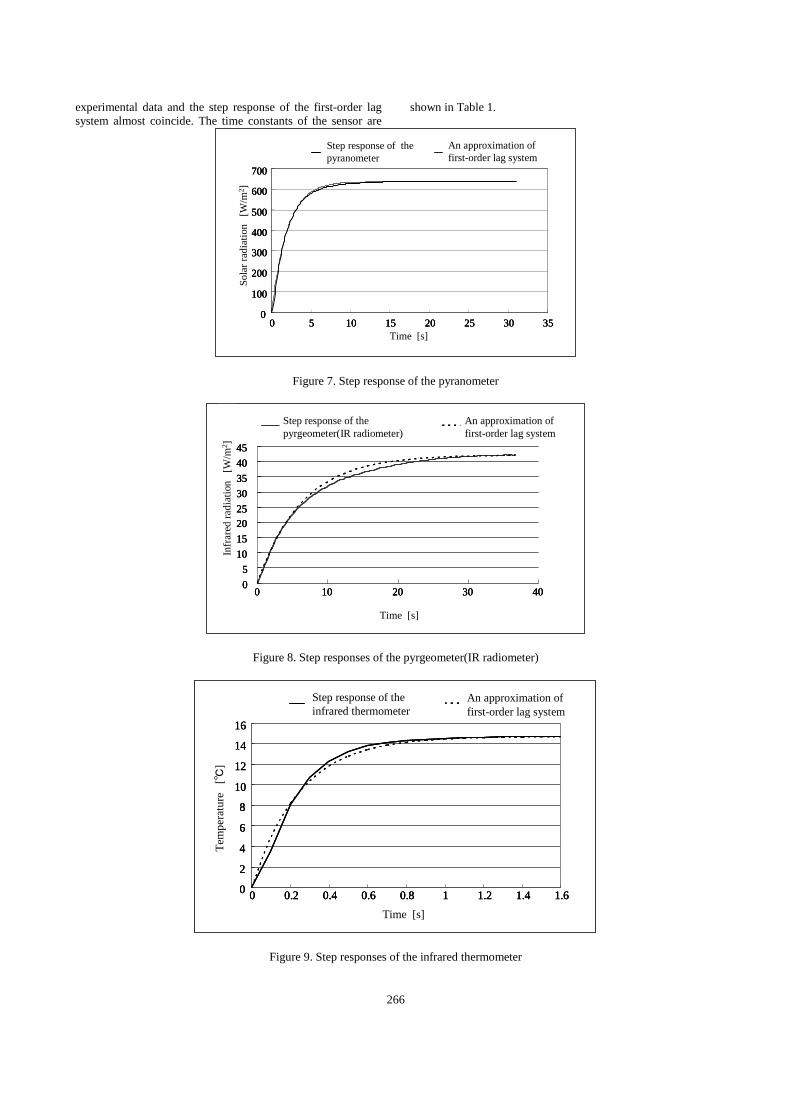
Time-Constant Measurement of the Sensor In regard to the pyranometer, pyrgeometer (IR

radiometer), infrared thermometer, and thermocouple, which are used to measure the thermal environment in an open space,

the results of the step response experiments are shown in Figures 7 through 10. The dynamic characteristics of each sensor are expressed as a first-order lag system. The

266

experimental data and the step response of the first-order lag system almost coincide. The time constants of the sensor are

shown in Table 1.

Step response of the pyranometer

An approximation of first-order lag system


Sola

r rad

iatio

n [

W/m

2 ]

Time [s]

0

100

200

300

400

500

600

700

0 5 10 15 20 25 30 35




Sola

r rad

iatio

n [

W/m

2 ]

Time [s]

0

100

200

300

400

500

600

700

0 5 10 15 20 25 30 35




Sola

r rad

iatio

n [

W/m

2 ]

Time [s]

0

100

200

300

400

500

600

700

0 5 10 15 20 25 30 35

Figure 7. Step response of the pyranometer

Step response of the pyrgeometer(IR radiometer)


Time [s]

Infr

ared

radi

atio

n [

W/m

2 ]

05

1015202530354045

0 10 20 30 40



Time [s]

Infr

ared

radi

atio

n [

W/m

2 ]

05

1015202530354045

0 10 20 30 40



Time [s]

Infr

ared

radi

atio

n [

W/m

2 ]

05

1015202530354045

0 10 20 30 40

Figure 8. Step responses of the pyrgeometer(IR radiometer)

Step response of the infrared thermometer


Tem

pera

ture

[℃

]

Time [s]

0

2

4

6

8

10

12

14

16

0 0.2 0.4 0.6 0.8 1 1.2 1.4 1.6



Tem

pera

ture

[℃

]

Time [s]

0

2

4

6

8

10

12

14

16

0 0.2 0.4 0.6 0.8 1 1.2 1.4 1.6



Tem

pera

ture

[℃

]

Time [s]

0

2

4

6

8

10

12

14

16

0 0.2 0.4 0.6 0.8 1 1.2 1.4 1.6

Figure 9. Step responses of the infrared thermometer

- 267 -

Figure 10. Step responses of the thermocouple

Table 1. Time constants of the sensors

Time constant[s]2

6.70.25

φ0.1 1.1φ0.3 2.6

Pyranometer MS-802he pyrgeometer(IR radiometer) MS-20

Infrared thermometer IRTS-P

T type thermocouple

Instruments

Experiment of Moving Measurement

The moving measurement experiment was conducted in a street running from east to west (Figure 11). Trees grow along the street. Figure 12 shows the installation positions of the sensors on the vehicle. A 10 km/h experiment started at 11:00 a.m. on October 12, 2005, and experiments were repeated at 20 km/h and 5 km/h (slow speed). The last experiment was run with a speed of 40 km/h at 11:19 a.m. As examples, the measurement value of the pyranometer with a time constant of 2.0 seconds and the measurement value of the pyrgeometer (IR radiometer) with the longest time constant of 6.7 seconds (Table 1) are accordingly shown in Figures 13 and 14. The horizontal axis was positioned in an east-west direction on the vehicle (i.e., the measurement value of longitude by the GPS). The vertical axis was the measurement value of the time when the GPS output the location signal. In Figure 13 and 14, a solid line indicates when the measuring vehicle was moving at the low speed of 5 km/h. In the case where the measuring vehicle was moving at this slow speed, the measurement value is considered as the true value f(x).

Next, when the vehicle moved repeatedly at speeds of 10, 20, and 40 km/h, the measuring data g(t) were shown against the moving distance position of the sensor. The difference between the spatial distribution of the measurement value and that of the true value (at 5km/h of moving speed) was

larger for the pyrgeometer (IR radiometer), which has a larger time constant (Figure 14), while the difference was smaller for the pyranometer, which has a smaller time constant (Figure 12). However, because the measurement was done repeatedly by changing the speed of the vehicle on the same road, and it took almost 20 minutes from the start to the end of the experiment, there is a possibility the measured properties were not in a steady state. In the case of pyrgeometer (IR radiometer), changes in infrared radiation level were observed during the experiment.

Figure 11. Where the moving measurement experiment was conducted

- 268 -

1000mm

1500

mm

Solar shadingAir temperature

GPSPyranometer

Infrared ray radiationPyrgeometer(IR radiometer)

Datalogger

Infrared thermometer

350m

m

1000mm

1500

mm


GPSPyranometer


Datalogger


350m

m

1000mm

1500

mm


GPSPyranometer


Datalogger


350m

m

Figure 12. Installed positions of the sensors

0

200

400

600

800

135.5095135.5105135.5115135.5125135.5135135.5145Longitude

Sola

r rad

iatio

n [W

/m2 ]

Low speed 10km/h 20km/h 40km/h Position of trees in the street

Figure 13. Moving measurement results for the pyranometer

360

380

400

420

440

135.5095135.5105135.5115135.5125135.5135135.5145

Longitude

Infr

ared

radi

atio

n[W

/m2 ]

Low speed 10km/h 20km/h 40km/h Position of trees in the street

Figure 14. Moving measurement results for the pyrgeometer(IR radiometer)

- 269 -

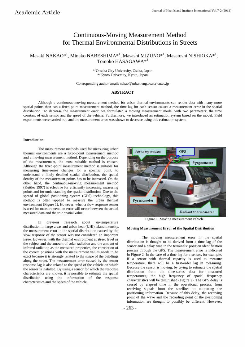
Estimated Results of the Spatial distribution and Evaluation

The spatial distribution f(x) is shown by the dashed line in Figures 15 and 16, which was estimated from equation (6) for the inverse system, equation (7) for a moving average to eliminate noises, and equation (9) for spatial changes. When the time constant of the pyranometer was 2.0 seconds, extremely favorable estimated results were obtained. In the case of the pyrgeometer (IR radiometer), although the estimated error became larger because of the large response lag when the time constant was 6.7 seconds, by taking into consideration the response lag of the sensor, the error was

decreased. The fluctuation of the estimated value reflects the fluctuations of the true value fairly well. However, the average level of estimated value was different from that of the true value, which seems to have been caused by the fact that both measurements were not carried out simultaneously. Because the time constant of the infrared thermometer was as short as 0.25 seconds, it was not necessary to apply this estimation method when the moving speed of the vehicle was 40 km/h or less.

0

100

200

300

400

500

600

700

800

900

1000

135.509135.51135.511135.512135.513135.514

全天

日射量

[W/m

2]

経度[°]

Sola

r rad

iatio

n [W

/m2 ]

Longitude

True value f(x)(measurement value at the low speed of 5 km/h)

The estimated value F(x), a dash line


Showing measured data at the speed of 40 km/h by the sensor position at measurement time

0

100

200

300

400

500

600

700

800

900

1000

135.509135.51135.511135.512135.513135.514

全天

日射量

[W/m

2]

経度[°]

Sola

r rad

iatio

n [W

/m2 ]

Longitude




Showing measured data at the speed of 40 km/h by the sensor position at measurement time

Figure 15. Comparative results of the moving measurement value, the true value, and the estimated value of the pyranometer

360

370

380

390

400

410

420

430

440

135.509135.51135.511135.512135.513135.514

赤外

放射

量[W

/m2]

経度[°]

Showing measured data at the speed of 40 km/h by the sensor position at a measurement time



Infr

ared

radi

atio

n [

W/m

2 ]

Longitude

360

370

380

390

400

410

420

430

440

135.509135.51135.511135.512135.513135.514

赤外

放射

量[W

/m2]

経度[°]




Infr

ared

radi

atio

n [

W/m

2 ]

Longitude

360

370

380

390

400

410

420

430

440

135.509135.51135.511135.512135.513135.514

赤外

放射

量[W

/m2]

経度[°]




Infr

ared

radi

atio

n [

W/m

2 ]




Infr

ared

radi

atio

n [

W/m

2 ]

Longitude

Figure 16. Comparative result of the moving measurement value, the true value and the estimated value of pyrgeometer (IR radiometer)

270

Conclusion

We suggested a method to estimate the spatial distribution from data that were obtained by continuously measuring the spatial thermal environmental distributions in streets, using sensors with a response lag and GPS with a time delay. In a street with roadside trees, the moving measurement was conducted at a continuous, steady speed of 40 km/h, using a pyranometer and a pyrgeometer (IR radiometer), which both have different response lags. Because we estimated the spatial distribution from the measured data, the measured error for the pyranometer with a 2.0-second time constant was extremely small. There was also an estimated error for the pyrgeometer (IR radiometer), which has a comparably large 6.7-second time constant, but by applying this method, it became obvious that the measurement error was effectively decreased.

References

W. Kuttler. 1997. “Climate and Air Hygiene Investigations for Urban Planning.” ACTA CLIMATOLOGICA. Universitatis Szegediensis, Tom. 31A

(Received Feb 9, 2012, Accepted Oct 10, 2012)

Documents

Continuous-Moving Measurement Method for Thermal ... · PDF fileContinuous-Moving Measurement Method for Thermal Environmental Distributions in Streets ... infrared thermometer,