Continuity of the poleward undercurrent along the eastern

Deep-Sea Research II 47 (2000) 811}829

Continuity of the poleward undercurrentalong the eastern boundary of the

mid-latitude north Paci"c

S.D. Pierce!,*, R.L. Smith!, P.M. Kosro!, J.A. Barth!,C.D. Wilson"

!College of Oceanic and Atmospheric Sciences, Oregon State University, 104 Ocean Administration Bldg.,Corvallis, OR 97331-5503, USA

"NOAA-NMFS, Seattle, WA 98115-0070, USA

Received 23 January 1998; received in revised form 10 November 1998; accepted 19 April 1999

Abstract

Several recent data sets improve our view of the poleward undercurrent of the CaliforniaCurrent System. As part of a triennial National Marine Fisheries Service (NMFS) survey ofPaci"c whiting, a series of 105 shipboard acoustic Doppler current pro"ler (ADCP) velocitysections across the shelf break from 33 to 513N at about 18 km meridional spacing werecollected from July to August 1995. Signi"cant ('0.05m s~1) subsurface poleward #owoccurred in 91% of the sections. A mean cross-shelf section using the entire data set hasstatistical signi"cance, revealing an undercurrent core '0.1m s~1 from 200}275m depth20}25km o! the shelf break. The mean poleward volume transport in a 125}325m layer is0.8$0.2]106 m3 s~1. We focus particular attention on the Cape Blanco to Cape Mendocinoregion, and the NMFS results are compared with shipboard ADCP three weeks later froma study of coastal upwelling processes near Cape Blanco. ADCP streamfunction maps arederived and strongly suggest that one portion of #ow is continuous over the 440km meridionalextent of the analysis region. Other portions of the #ow show evidence of o!shore turning,separation, and the formation of anti-cyclonic eddies. We also note that isopycnic potentialvorticity from alongslope CTD stations during the NMFS survey appears to be a tracer for thepoleward #ow. ( 2000 Elsevier Science Ltd. All rights reserved.

*Corresponding author.E-mail address: [email protected] (S.D. Pierce)

0967-0645/00/$ - see front matter ( 2000 Elsevier Science Ltd. All rights reserved.PII: S 0 9 6 7 - 0 6 4 5 ( 9 9 ) 0 0 1 2 8 - 9

1. Introduction

Subsurface poleward #ow occurs along all "ve major oceanic eastern boundaries.At mid-latitudes, this poleward #ow opposes the equatorward subtropical easternboundary current #ow at the surface. During the coastal upwelling season, thepoleward #ow also opposes intense equatorward surface-intensi"ed upwelling jets.These undercurrents are usually found over the continental slope and have typicalalongshore speeds of 0.1}0.3m s~1 and a depth range 100}300m (Neshyba et al., 1989;Warren, 1990). Since they have volume transports of O(1)]106 m3 s~1, they may besigni"cant oceanic features in a global circulation context, besides being importantaspects of eastern boundary regions.

Although the poleward undercurrent in the California Current System has been thebest observed and most studied of any, several basic dynamic and kinematic issuesremain unresolved (e.g. Warren, 1990). Some of the outstanding kinematic questionsconcern the undercurrent's continuity in both space and time. Most historical obser-vations have consisted of individual cross-shore hydrographic sections and relativelyshort current meter records. Some of the most interesting recent observations of thepoleward undercurrent have been Lagrangian measurements using subsurfaceRAFOS drifters (Collins et al., 1996a). These measurements unambiguously demon-strate the continuity of the poleward #ow at about 140m depth over a 500km pathfrom 37.8 to 41.83N.

The 1995 triennial acoustic-trawl survey by the National Marine FisheriesService (NMFS), to assess the abundance and distribution of Paci"c whiting,included shipboard acoustic Doppler current pro"ler (ADCP) velocities,which we examine here. The "sheries results are reported by Wilson andGuttormsen (1997). The e!ects of currents on Paci"c whiting are also underinvestigation and will be reported elsewhere. The survey sampled the entiremid-latitude eastern Paci"c slope in July}August 1995, with cross-slopetransects running nominally from 50 to 1500 m isobaths at 18 km meridionalspacing (Fig. 1). Although the cruise plan was largely determined from"sheries considerations, the data set is also well-suited to studying the polewardundercurrent.

The meridional extent of the NMFS ADCP data allows us to address issuesof spatial continuity and latitudinal variation. Also in 1995, three weeks afterthe NMFS survey passed Oregon, an intensive SeaSoar/ADCP survey studiedupwelling processes at Cape Blanco (Barth et al., 2000; Barth and Smith, 1998).We present some results from this survey, which observed strong interac-tion between the poleward undercurrent and a separating coastal upwelling jetabove.

In the presence of tidal currents and inertial oscillations, and with little concur-rent cross-shore hydrographic data, we seek to detect the subtidal and relativelystable and geostrophic poleward undercurrent. We accomplish this primarilyusing two methods: averaging together many cross-shore sections to reduce the`noisea, and deriving streamfunction to help reveal the non-divergent subtidalvelocity "eld.

812 S.D. Pierce et al. / Deep-Sea Research II 47 (2000) 811}829

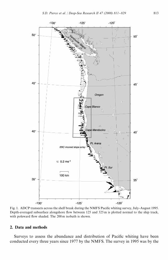
Fig. 1. ADCP transects across the shelf break during the NMFS Paci"c whiting survey, July}August 1995.Depth-averaged subsurface alongshore #ow between 125 and 325m is plotted normal to the ship track,with poleward #ow shaded. The 200m isobath is shown.

2. Data and methods

Surveys to assess the abundance and distribution of Paci"c whiting have beenconducted every three years since 1977 by the NMFS. The survey in 1995 was by the

S.D. Pierce et al. / Deep-Sea Research II 47 (2000) 811}829 813

R/V Miller Freeman and included acoustic echo measurements at two frequencies (38and 120 kHz) using a Simrad EK500 system, as well as trawl work. The complete1 July}1 September 1995 survey included a fast run down to the southern end fromSeattle at the beginning and additional transects from 52 to 553N o! the QueenCharlotte Islands at the end. Results here use data from 7 July to 28 August between33 and 513N (Fig. 1). Nominal meridional spacing of these 105 mostly east}west lineswas 18 km, and the mean length of a transect was 52 km. Transects generally ranmid-shelf to mid-slope, between the 50 and 1500 m isobaths, sometimes extending todeeper water depending on real-time biological scattering results (Wilson and Guttor-msen, 1997). CTD casts were made at selected trawl sites and at two or three locationsalong every second or third transect, down to depths of about 500m. For the "rsttime, this Paci"c whiting survey also included acoustic Doppler current pro"ler(ADCP) velocity measurements.

The CTD data are used to compute `spicinessa as de"ned by Flament (1986). Spici-ness is approximately perpendicular to ph in a ¹}S diagram and works well in theCalifornia Current System because average ¹}S curves lie roughly orthogonal to iso-pycnals (Tibby, 1941). High spiciness corresponds to high temperature or high salinity,while low spiciness corresponds to low temperature or low salinity. Temperature andsalinity, hence spiciness, on subsurface isopycnals can be assumed to be conservative.Density anomaly sigma}theta (ph) was calculated using the 1980 EOS algorithms.

An RD Instruments 153.6 kHz narrow-band, hull-mounted ADCP measuredcurrents throughout the survey. We used a vertical bin width of 8m, pulse length of8m, and an ensemble averaging time of 2.5min. Pings per ensemble varied from 66 to101, and the depth range of good data (good pings '30%) was typically 22}326m.Details of ADCP data processing generally follow the methods used for the R/VWecoma Cape Blanco study (Barth et al., 2000), which are contained in the data reportPierce et al. (1997). Data were required to pass tests of su$cient return signal,acceptable second derivatives of u, v, and w with respect to depth, and reasonable errorvelocities, as recommended by Firing et al. (1995) and Zedel and Church (1987). TheADCP was slaved to the EK500 biological instrument to avoid interference. Pre-cruise tests revealed no interference between the two instruments when the ADCPobtained ship velocity from navigation alone. The ADCP bottom-tracking feature,however, which puts more energy into the water, was found to cause an arti"cialsignal on the EK500. For this reason, bottom tracking was never enabled throughoutthe survey. GPS P-code (military-type) navigation was used for position and gyro-compass for heading, to determine absolute velocities. The ADCP/navigation/gyro-compass system was calibrated by covariability between currents and ship velocity(Kosro, 1985; Pollard and Read, 1989). A scale factor of 2% and a calibration error,which varied linearly in time from 0.1 to 0.53, were detected and removed. Remainingcalibration uncertainty implies an unknown bias of 0.02m s~1 in absolute velocities.Raw reference layer velocities were low-pass "ltered with a 20min Blackman window(Firing et al., 1995). Short-term inherent random errors for an ensemble are at most0.02ms~1, and the estimated rms error in absolute reference layer velocity is 0.04ms~1.

Sections of ADCP were contoured using a four-pass Barnes objective analysis (OA)scheme (Barnes, 1994; Daley, 1991). The Barnes scheme, widely used in atmospheric


science, applies a Gaussian-weighted average successively, converging towards theobserved points. The method is related to statistical optimal interpolation, but issimpler and more #exible and does not require prior speci"cation of a covariancemodel for the observed "eld. Statistical optimal interpolation is only `optimala fora given covariance model; the lack of su$cient historical data frequently makesdetermination of the appropriate model di$cult. Four Barnes iterations were su$-cient, since at this point the gridded values were changing (0.01m s~1 rms. We holdthe Barnes radii constant at 7.5 km in the horizontal and 25m in the vertical; scaleslarger than these are not smoothed.

We de"ne an approximate alongshore direction to be 3303T south of 40.23N andnorth of 483N, and 03T from 40.2 to 483N. For maps of ADCP vectors, componentvalues and locations are 5 km spatial averages, and in cases where the cruise trackoverlays itself, measurements from di!erent times are averaged together.

We derive streamfunction from the ADCP velocities. This helps reveal the under-current by reducing the aliasing e!ects of tidal and inertial signals. First, the twocomponents of velocity are gridded using a four-pass Barnes OA (Barnes, 1994). Boththe alongshore and the o!shore Barnes radii are kept constant at 18 km, which is thealongshore sampling interval. This choice minimizes unnecessary smoothing of theresulting "elds, which is appropriate here since we are deriving streamfunction asa descriptive tool, rather than selecting certain length scales based on dynamical ideas.We determine streamfunction over this gridded velocity "eld using the version IIImethod of Hawkins and Rosenthal (1965), introduced to the oceanographic commun-ity by Carter and Robinson (1987). A Poisson equation for the velocity potential,forced by the observed "eld of divergence (calculated for each grid box), is solved witha boundary condition of zero on all sides. The resulting velocity potential is then usedto add a correction to the boundary conditions for the Poisson equation for thestreamfunction, forced by the relative vorticity "eld. This approach has the e!ect ofmaximizing the amount of kinetic energy in the resulting streamfunction "eld. We usethe Poisson solver developed by Cummins and Vallis (1994), which handles theirregular boundary condition of no normal #ow into the coast. Attempting to use theobserved velocity "eld directly as a boundary condition for the streamfunctioncalculation, the simplest approach (e.g. Pollard and Regier, 1992; Allen and Smeed,1996), implicitly assumes that the observed "eld along the boundary is non-divergent,which may not be true given measurement noise. Non-divergent vectors are derivedfrom the gridded streamfunction and then interpolated back to their original locationsusing improved Akima bivariate interpolation (Akima, 1996). The Barnes OA and thestreamfunction derivation together amount to a method of systematically applyingconservation of mass throughout a region.

3. Southern California to Vancouver Island

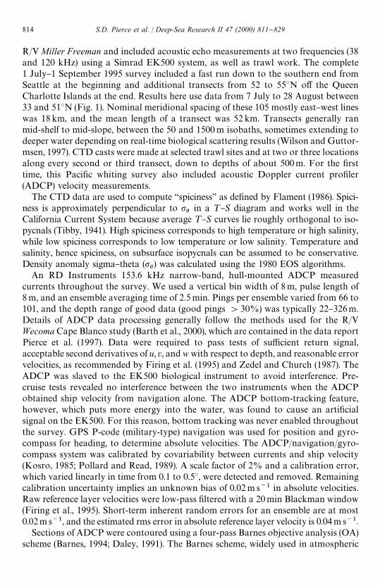
The full set of 105 alongshore velocity sections from the NMFS survey are availablefor viewing in an on-line data report (Pierce, 1997). Here we present a representativesample of 16 sections (Fig. 2a and b). As expected during the summer upwellingseason, surface equatorward #ow is frequently present. Signi"cant surface-intensi"ed



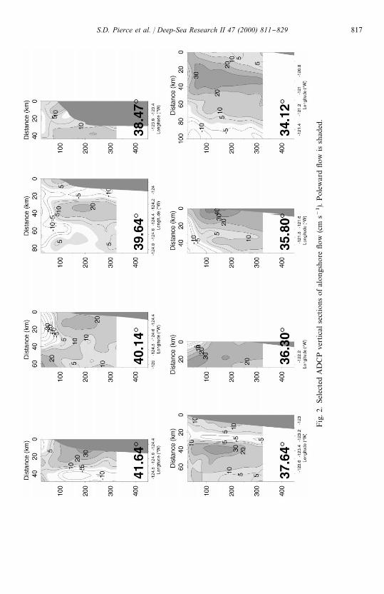
Fig

.2.

Sele

cted

AD

CP

vert

ical

sect

ions

ofal

ongs

hore#ow

(cm

s~1)

.Pole

war

d#ow

issh

aded

.


equatorward jets associated with upwelling can be seen at 48.33N, 42.973N, 42.143N,and 40.143. Consistent with historical observations and satellite imagery (Smith,1995), the upwelling jets to the north of 42.83N (Cape Blanco, Oregon) appear to becon"ned inshore of the continental shelf break. In sections to the south of 42.83N, theupwelling jets can be found seaward of the shelf break. The separation, that occurs asan upwelling jet passes through this region, can be seen by comparing the 42.973N and42.143N sections. Observation of the details of this separation process was themotivation for the Cape Blanco study (Fig. 7; Barth et al., 2000). Outside of thisregion, the absence of many cross-shore hydrographic observations to complementthe NMFS ADCP makes further interpretation of the surface #ows di$cult. In thispaper we focus on the subsurface poleward #ow.

The ubiquity of poleward #ow throughout the 5400 km of cross-shore trackline isstriking. Individual sections show complex poleward current patterns (Fig. 2). Baro-tropic tidal currents, baroclinic tidal currents, and inertial oscillations are probably allpresent in any particular section, a 0.05}0.10m s~1 contribution (Torgrimson andHickey, 1979) which confuses the view of the subtidal and geostrophic signal.

As one method of summarizing this large data set, we consider a subsurface depth-averaged layer from 125 to 325m (Fig. 1). We chose this layer de"nition as a reason-able one to focus our attention on the subsurface poleward undercurrent.Depth-averaged poleward #ow within this subsurface layer appears as black shadingin Fig. 1. In 96 out of 105 sections, maximum velocity is at least 0.05m s~1 over a5km width. The mean of the maximum core layer velocities seen at each section is0.18$0.01m s~1.

3.1. Mean structure

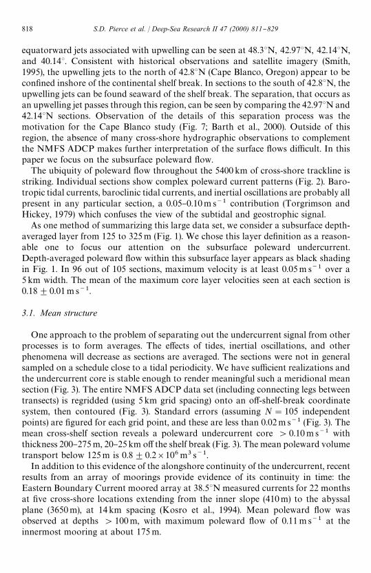
One approach to the problem of separating out the undercurrent signal from otherprocesses is to form averages. The e!ects of tides, inertial oscillations, and otherphenomena will decrease as sections are averaged. The sections were not in generalsampled on a schedule close to a tidal periodicity. We have su$cient realizations andthe undercurrent core is stable enough to render meaningful such a meridional meansection (Fig. 3). The entire NMFS ADCP data set (including connecting legs betweentransects) is regridded (using 5 km grid spacing) onto an o!-shelf-break coordinatesystem, then contoured (Fig. 3). Standard errors (assuming N"105 independentpoints) are "gured for each grid point, and these are less than 0.02m s~1 (Fig. 3). Themean cross-shelf section reveals a poleward undercurrent core '0.10 m s~1 withthickness 200}275m, 20}25km o! the shelf break (Fig. 3). The mean poleward volumetransport below 125m is 0.8$0.2]106m3 s~1.

In addition to this evidence of the alongshore continuity of the undercurrent, recentresults from an array of moorings provide evidence of its continuity in time: theEastern Boundary Current moored array at 38.53N measured currents for 22 monthsat "ve cross-shore locations extending from the inner slope (410m) to the abyssalplane (3650m), at 14km spacing (Kosro et al., 1994). Mean poleward #ow wasobserved at depths '100m, with maximum poleward #ow of 0.11 m s~1 at theinnermost mooring at about 175 m.


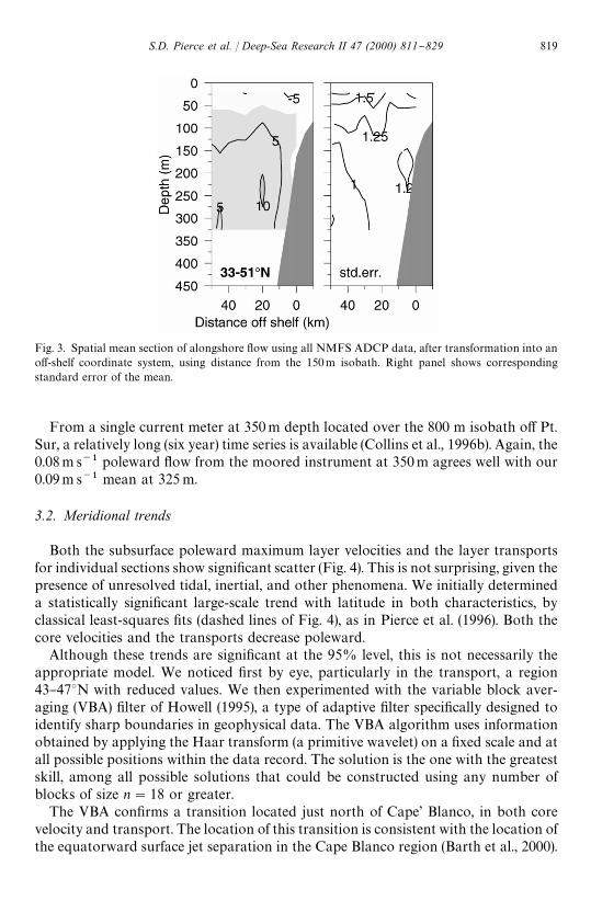
Fig. 3. Spatial mean section of alongshore #ow using all NMFS ADCP data, after transformation into ano!-shelf coordinate system, using distance from the 150m isobath. Right panel shows correspondingstandard error of the mean.

From a single current meter at 350m depth located over the 800 m isobath o! Pt.Sur, a relatively long (six year) time series is available (Collins et al., 1996b). Again, the0.08m s~1 poleward #ow from the moored instrument at 350m agrees well with our0.09m s~1 mean at 325 m.

3.2. Meridional trends

Both the subsurface poleward maximum layer velocities and the layer transportsfor individual sections show signi"cant scatter (Fig. 4). This is not surprising, given thepresence of unresolved tidal, inertial, and other phenomena. We initially determineda statistically signi"cant large-scale trend with latitude in both characteristics, byclassical least-squares "ts (dashed lines of Fig. 4), as in Pierce et al. (1996). Both thecore velocities and the transports decrease poleward.

Although these trends are signi"cant at the 95% level, this is not necessarily theappropriate model. We noticed "rst by eye, particularly in the transport, a region43}473N with reduced values. We then experimented with the variable block aver-aging (VBA) "lter of Howell (1995), a type of adaptive "lter speci"cally designed toidentify sharp boundaries in geophysical data. The VBA algorithm uses informationobtained by applying the Haar transform (a primitive wavelet) on a "xed scale and atall possible positions within the data record. The solution is the one with the greatestskill, among all possible solutions that could be constructed using any number ofblocks of size n"18 or greater.

The VBA con"rms a transition located just north of Cape' Blanco, in both corevelocity and transport. The location of this transition is consistent with the location ofthe equatorward surface jet separation in the Cape Blanco region (Barth et al., 2000).


Fig. 4. Maximum poleward < (]) and the total subsurface layer transport (v), for each NMFS ADCPsection. Light and bold solid lines show variable block averages for the maximum < and transportrespectively. Light and bold dashed lines are least-squares "ts.

Anticipating the results of the next section as seen in Fig. 7, and discussed in detail inBarth et al. (2000), a separating coastal jet can strengthen and deepen to the pointwhere it interacts signi"cantly with the poleward undercurrent. To the north of 473N,core velocity and transport are similar to what they were to the south of Cape Blanco.Excluding 43}473N, we see only a small decrease in the core velocity and transport ofabout 1% per degree of latitude.

The characteristic width of the undercurrent (de"ned as the width at half-maximumvelocity) and its change with latitude are revealed by forming three mean sections(Fig. 5). Using two 53 latitude bands to the south of Cape Blanco and one 43 band tothe north, a narrowing of the undercurrent to poleward is evident, although barelystatistically signi"cant given uncertainties in width estimation (probably $5 km).Consistent with the undercurrent hugging the slope, the core moves closer to the slopeas it narrows. The "rst-baroclinic Rossby radii of deformation for these latitudebands, as calculated by Chelton et al. (1998) from climatological 13 gridded hydro-graphic data, are 24.3, 21.8, and 15.5 km (Fig. 5, horizontal lines). The widths of thepoleward #ow are consistent with the Rossby radii, which has also been noted in thecase of the Peru undercurrent (Huyer, 1980). The change in width is not connectedwith a change in bottom slope, which does not change systematically with latitude.


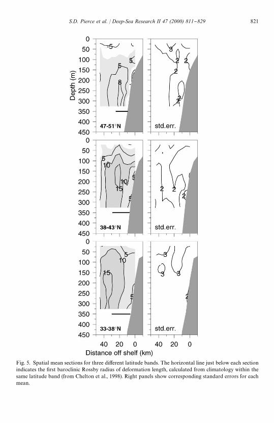
Fig. 5. Spatial mean sections for three di!erent latitude bands. The horizontal line just below each sectionindicates the "rst baroclinic Rossby radius of deformation length, calculated from climatology within thesame latitude band (from Chelton et al., 1998). Right panels show corresponding standard errors for eachmean.


The "rst-baroclinic Rossby radius is a natural length scale in the ocean, and it is oftenassociated with widths of boundary phenomena such as coastal upwelling, Kelvinwaves, etc. It is not surprising that the poleward undercurrent #ow appears to berelated to this scale as well.

4. Cape Mendocino to Cape Blanco

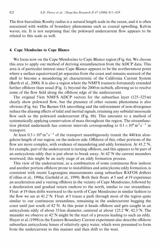
We focus now on the Cape Mendocino to Cape Blanco region (Fig. 6a). We choosethis area to apply our method of deriving streamfunction from the ADCP data. Thisarea is of particular interest since Cape Blanco appears to be the northernmost pointwhere a surface equatorward jet separates from the coast and remains seaward of theshelf to become a meandering jet characteristic of the California Current System(Barth et al., 2000). It is also a region where the NMFS transects fortunately extendedfurther o!shore than usual (Fig. 1), beyond the 2000m isobath, allowing us to resolvesome of the #ow "eld along the o!shore edge of the undercurrent.

The original 5 km NMFS ADCP vectors for the subsurface layer (125}325m)clearly show poleward #ow, but the presence of other oceanic phenomena is alsoobvious (Fig. 6a). The Barnes OA smoothing and the enforcement of non-divergencereduce the aliasing e!ects of tidal and inertial signals, retaining any subtidal mesoscale#ow such as the poleward undercurrent (Fig. 6b). This amounts to a method ofsystematically applying conservation of mass throughout the region. The streamfunc-tion plotted underneath has contour intervals corresponding to 0.1]106m3 s~1 intransport.

At least 0.3]106m3 s~1 of the transport unambiguously transit the 440 km alon-gshore length of our region, on the inshore side. O!shore of this, other portions of the#ow are more complex, with evidence of meandering and eddy formation. At 41.23N,for example, part of the undercurrent is turning o!shore, and this appears to be part ofan anticyclonic eddy that is just about to break away. At 423N the current meanderswestward; this might be an early stage of an eddy formation process.

This view of the undercurrent, as a combination of some continuous #ow inshoreand another portion o!shore prone to instabilities and anticylconic eddy formation, isconsistent with recent Lagrangian measurements using subsurface RAFOS drifters(Collins et al., 1996a; Gar"eld et al., 1999). Both their #oats d5 and d19 experiencean acceleration and a veering o!shore in the vicinity of Cape Mendocino, followed bya deceleration and gradual return onshore to the north, similar to our streamlines.Float d19 then drifts westward to the north of Cape Mendocino in similar fashion tothe #ow we see at 41.23N. Float d5 traces a path through most of the region quitesimilar to our continuous streamlines, remaining in the undercurrent hugging thecoast until just south of 423N. At this point it heads o!shore and gets caught in ananticyclonic eddy of about 35 km diameter, centered at about 125.23W, 42.33N. Themeander we observe at 423N might be the start of a process leading to such an eddy.Huyer et al. (1998) in the Eastern Boundary Current experiment also describe o!shoresubsurface anticyclonic lenses of relatively spicy water, which were presumed to formfrom the undercurrent in this manner and then drift to the west.


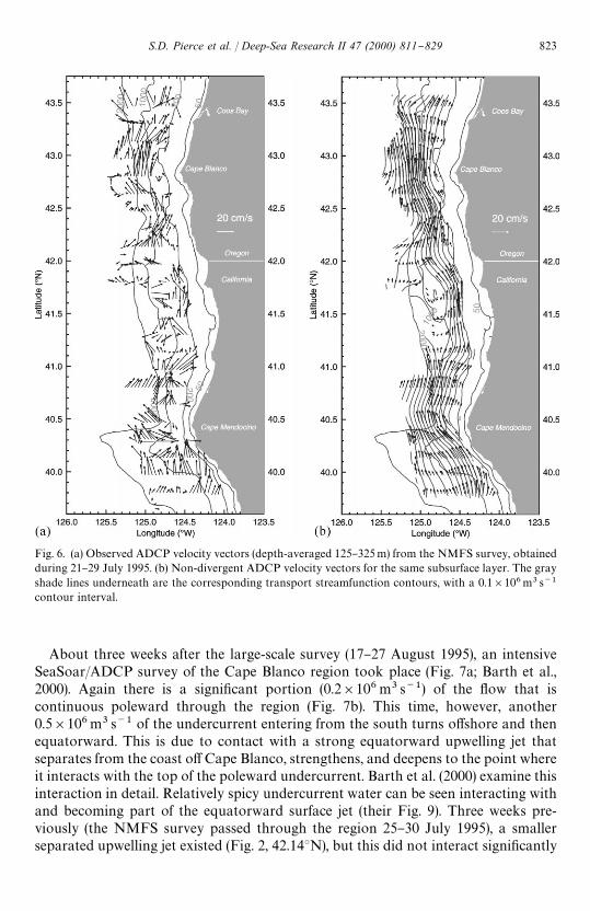
Fig. 6. (a) Observed ADCP velocity vectors (depth-averaged 125}325m) from the NMFS survey, obtainedduring 21}29 July 1995. (b) Non-divergent ADCP velocity vectors for the same subsurface layer. The grayshade lines underneath are the corresponding transport streamfunction contours, with a 0.1]106m3 s~1

contour interval.

About three weeks after the large-scale survey (17}27 August 1995), an intensiveSeaSoar/ADCP survey of the Cape Blanco region took place (Fig. 7a; Barth et al.,2000). Again there is a signi"cant portion (0.2]106 m3 s~1) of the #ow that iscontinuous poleward through the region (Fig. 7b). This time, however, another0.5]106m3 s~1 of the undercurrent entering from the south turns o!shore and thenequatorward. This is due to contact with a strong equatorward upwelling jet thatseparates from the coast o! Cape Blanco, strengthens, and deepens to the point whereit interacts with the top of the poleward undercurrent. Barth et al. (2000) examine thisinteraction in detail. Relatively spicy undercurrent water can be seen interacting withand becoming part of the equatorward surface jet (their Fig. 9). Three weeks pre-viously (the NMFS survey passed through the region 25}30 July 1995), a smallerseparated upwelling jet existed (Fig. 2, 42.143N), but this did not interact signi"cantly


Fig. 7. (a) Observed ADCP velocity vectors (depth-averaged 125}325m) from the Coastal Jet Separationduring 17}27 August 1995 cruise. (b) Non-divergent ADCP velocity vectors for the same subsurface layer.The gray shade lines underneath are the corresponding transport streamfunction contours, witha 0.1]106m3 s~1 contour interval.

with the undercurrent. The interaction with a strong separating surface jet above isanother mechanism for a portion of the undercurrent to turn o!shore.

5. Alongslope hydrography

As part of the NMFS survey, CTD casts were made at two or three locationsalong every second or third transect, down to depths of about 500m. We selectedthe 31 stations out of the total of 65 that were on the slope (bottom depths245}1830m) to characterize the meridional water mass properties of the undercur-rent. The core of spicy water at 100}250m at the southern end of the survey spreadsto poleward and is still detectable as a spiciness maximum in the vertical at thenorthern end of the survey, at 150}225m depth (Fig. 8a). Several examples of thistype of indirect evidence for poleward undercurrent #ow can be found in Neshybaet al. (1989).

The Cape Blanco study made a cross-slope CTD section at 43.23N, the FM line(Fig. 9a). Here the down-warped ph"26.6 isopycnal close to the slope indicates thepresence of poleward geostrophic #ow, and the spiciness maximum con"rms thesouthern source of this undercurrent #ow.

Also shown in Fig. 8a (small triangles) is the depth of the center of mass of poleward#ow from ADCP. This is calculated as z

#."+vz/+v over the subsurface layer, where

v is a raw poleward ADCP velocity and z is the depth of that measurement, providinga good indication of the core undercurrent depth. We note that z

#.ranges from 150 to


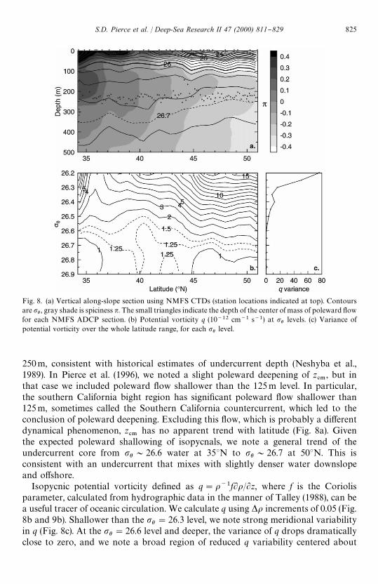
Fig. 8. (a) Vertical along-slope section using NMFS CTDs (station locations indicated at top). Contoursare ph , gray shade is spiciness n. The small triangles indicate the depth of the center of mass of poleward #owfor each NMFS ADCP section. (b) Potential vorticity q (10~12 cm~1 s~1) at ph levels. (c) Variance ofpotential vorticity over the whole latitude range, for each ph level.

250m, consistent with historical estimates of undercurrent depth (Neshyba et al.,1989). In Pierce et al. (1996), we noted a slight poleward deepening of z

#., but in

that case we included poleward #ow shallower than the 125m level. In particular,the southern California bight region has signi"cant poleward #ow shallower than125m, sometimes called the Southern California countercurrent, which led to theconclusion of poleward deepening. Excluding this #ow, which is probably a di!erentdynamical phenomenon, z

#.has no apparent trend with latitude (Fig. 8a). Given

the expected poleward shallowing of isopycnals, we note a general trend of theundercurrent core from ph&26.6 water at 353N to ph&26.7 at 503N. This isconsistent with an undercurrent that mixes with slightly denser water downslopeand o!shore.

Isopycnic potential vorticity de"ned as q"o~1fLo/Lz, where f is the Coriolisparameter, calculated from hydrographic data in the manner of Talley (1988), can bea useful tracer of oceanic circulation. We calculate q using *o increments of 0.05 (Fig.8b and 9b). Shallower than the ph"26.3 level, we note strong meridional variabilityin q (Fig. 8c). At the ph"26.6 level and deeper, the variance of q drops dramaticallyclose to zero, and we note a broad region of reduced q variability centered about


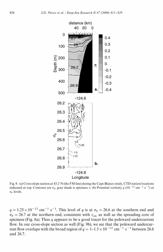
Fig. 9. (a) Cross-slope section at 43.23N (the FM line) during the Cape Blanco study, CTD station locationsindicated at top. Contours are ph , gray shade is spiciness n. (b) Potential vorticity q (10~12 cm~1 s~1) atph levels.

q"1.25]10~12 cm~1 s~1. This level of q is at ph"26.6 at the southern end andph"26.7 at the northern end, consistent with z

#.as well as the spreading core of

spiciness (Fig. 8a). Thus q appears to be a good tracer for the poleward undercurrent#ow. In our cross-slope section as well (Fig. 9b), we see that the poleward undercur-rent #ow overlaps with the broad region of q"1}1.5]10~12 cm~1 s~1 between 26.6and 26.7.


This should not be surprising, since if we believe some part of the undercurrent to becontinuous over this great range of latitude, it must have some mechanism forconserving its potential vorticity in the face of the signi"cant change in planetaryvorticity f. The way the undercurrent conserves q is by a slight thickening, a polewardincrease in *z between isopycnals, to counteract increasing f. Although we haveneglected the e!ects of relative vorticity, we expect this to be a possibly importantterm in the undercurrent only in a local sense.

6. Summary

From this extensive set of NMFS ADCP data collected during July}August 1995,with supporting evidence from the intensive Cape Blanco study in August 1995, animproved view of the poleward undercurrent emerges. The undercurrent is presentalong almost the entire mid-latitude eastern boundary of the North Paci"c, witha mean maximum velocity of 0.18m s~1, overall mean of 0.10m s~1, core depth200}275m, mean location 20}25km o! the shelf break, width of about a Rossbyradius, and 125}325m transport of 0.8$0.2]106m3 s~1. ADCP streamfunctionmaps derived from velocity observations between Cape Blanco, Oregon, and CapeMendocino, California, show some continuity of the undercurrent over this 440 kmlong region. In other portions of the #ow, undercurrent water appears to leave theslope, thus breaking continuity on scales greater than about 300km, in the formof anticyclonic eddies or as a portion of a separated equatorward jet in the vicinityof Cape Blanco. Analysis of alongshore hydrographic data provides additionalevidence of continuity, particularly at levels below ph"26.6}26.7. Potentialvorticity in the range 1}1.5]10~12 cm~1 s~1 appears to be a good tracer of thepoleward #ow.

Acknowledgements

We thank Jane Huyer for helpful discussions. This work was supported by theO$ce of Naval Research grants N00014-9610039, -9810026, -92J1357, and -91J1242,with additional support from National Science Foundation grant OCE-9314370.

References

Akima, H., 1996. Rectangular-grid-data surface "tting that has the accuracy of a bicubic polynomial. ACMTransactions on Mathematical Software 22, 357}361.

Allen, J.T., Smeed, D.A., 1996. Potential vorticity and vertical velocity at the Iceland-Faeroes front. Journalof Physical Oceanography 26, 2611}2634.

Barnes, S.L., 1994. Applications of the Barnes objective analysis scheme, part III: tuning for minimum error.Journal of Atmospheric and Oceanic Technology 11, 1459}1470.

Barth, J.A., Pierce, S.D., Smith, R.L., 2000. A separating coastal upwelling jet at Cape Blanco, Oregon andits connection to the California Current System. Deep-Sea Research II 47, 783}810.


Barth, J.A., Smith, R.L., 1998. Separation of a coastal upwelling jet at Cape Blanco, Oregon, USA. SouthAfrican Journal of Marine Science 19, 5}14.

Carter, E.F., Robinson, A.R., 1987. Analysis models for the estimation of oceanic "elds. Journal ofAtmospheric and Oceanic Technology 4, 49}74.

Chelton, D.B., deSzoeke, R.A., Schlax, M.G., El Naggar, K., Siwertz, N., 1998. Geographical variability ofthe "rst-baroclinic Rossby radius of deformation. Journal of Physical Oceanography 28, 433}460.

Collins, C.A., Gar"eld, N., Paquette, R.G., Carter, E., 1996a. Lagrangian measurement of subsurfacepoleward #ow between 383N and 433N along the west coast of the United States during summer, 1993.Geophysical Research Letters 23, 2461}2464.

Collins, C.A., Paquette, R.G., Ramp, S.R., 1996b. Annual variability of ocean currents at 350-m depth overthe continental slope o! Pt. Sur, California. CalCOFI Reports 37, 257}263.

Cummins, P.F., Vallis, G.K., 1994. Algorithm 732: solvers for self-adjoint elliptic problem in irregulartwo-dimensional domains. ACM Transactions Mathematical Software 20, 247}261.

Daley, R., 1991. Atmospheric Data Analysis. Cambridge Press, Cambridge, 457pp.Firing, E., Ranada, J., Caldwell, P., 1995. Processing ADCP data with the CODAS software system version

3.1, User's manual. (Manual and software available electronically at ftp://noio.soest.hawaii.edu/pub/codas3.)

Flament, P., 1986. Finestructure and subduction associated with upwelling "laments. Ph.D. Thesis,University of California, San Diego.

Gar"eld, N., Collins, C.A., Paquette, R.G., Carter, A., 1999. Lagrangian exploration of the Californiaundercurrent, 1992}1995. Journal of Physical Oceanography 29, 560}583.

Hawkins, H.F., Rosenthal, S.L., 1965. On the computation of streamfunctions from the wind "eld. MonthlyWeather Review 93, 245}252.

Howell, J.F., 1995. Identifying sudden changes in data. Monthly Weather Review 123, 1207}1212.Huyer, A., 1980. The o!shore structure and subsurface expression of sea level variations o! Peru, 1976}77.

Journal of Physical Oceanography 10, 1755}1768.Huyer, A., Barth, J.A., Kosro, P.M., Shearman, R.K., Smith, R.L., 1998. Upper-ocean water mass character-

istics of the California Current, summer 1993. Deep-Sea Research 45, 1411}1442.Kosro, P.M., 1985. Shipboard acoustic pro"ling during the Coastal Ocean Dynamics Experiment. Ph.D.

Thesis, SIO Ref. 85-8, Scripps Institute of Oceanography, La Jolla, CA, 119pp.Kosro, P.M., Ramp, S.R., Smith, R.L., 1994. Moored current measurements over the continental slope in

EBC: a "rst look. Transactions, American Geophysical Union, EOS 75 (44), 345.Neshyba, S.J., Mooers, C.N.K., Smith, R.L., Barber, R.T. (Eds.), 1989. Poleward Flows along Eastern Ocean

Boundaries. Springer, New York.Pierce, S.D., Smith, R.L., Kosro, P.M., 1996. Observations of the poleward undercurrent along the

eastern boundary of the mid-latitude Paci"c. Transactions, American Geophysical Union, EOS 77 (46),F345.

Pierce, S.D., Barth, J.A., Smith, R.L., 1997. Acoustic Doppler Current Pro"ler observations during theCoastal Jet Separation project on R/V Wecoma, 17}27 August 1995. College of Oceanic and Atmo-spheric Sciences, Oregon State University, Data Rep. 166, Ref. 97-4, 123pp.

Pierce, S.D., 1997. Observations of the poleward undercurrent along the eastern boundary of the mid-latitude Paci"c. [Data report, available on-line from http://diana.oce.orst.edu.]

Pollard, R., Read, J., 1989. A method for calibrating ship mounted acoustic Doppler pro"lers and thelimitations of gyro compasses. Journal of Atmospheric and Oceanic Technology 6, 859}865.

Pollard, R., Regier, L., 1992. Vorticity and vertical circulation at an ocean front. Journal of PhysicalOceanography 22, 609}625.

Smith, R.L., 1995. The physical processes of coastal upwelling systems. In: Summerhayes, C.P., Emeis,K.-C., Angel, M.V., Smith, R.L., Zeitzshel, B. (Eds.), Upwelling in the Ocean: Modern Processes andAncient Records. Wiley, New York, pp. 39}64.

Talley, L.D., 1988. Potential vorticity distribution in the North Paci"c. Journal of Physical Oceanography18, 89}106.

Tibby, R.B., 1941. The water masses o! the west coast of North America. Journal of Marine Research 4,112}121.


Torgrimson, G.M., Hickey, B.M., 1979. Barotropic and baroclinic tides over the continental slope and shelfo! Oregon. Journal of Physical Oceanography 9, 945}961.

Warren, B.A., 1990. Book review of Poleward #ows along eastern ocean boundaries. Limnology andOceanography 35, 1219}1220.

Wilson, C.D., Guttormsen, M.A., 1997. Echo integration-trawl survey of Paci"c Whiting, Merlucciusproductus, o! the west coasts of the United States and Canada during July}September 1995. NOAATechnical Memo NMFS-AFSC-74, NOAA-NMFS, US Department of Commerce.

Zedel, L.J., Church, J.A., 1987. Real-time screening techniques for Doppler current pro"ler data. Journal ofAtmospheric and Oceanic Technology 4, 572}581.


Documents

Continuity of the poleward undercurrent along the eastern