Embed Size (px)
Citation preview

EXTENSION CENTER FOR COMMUNITY VITALITY
Continuing the Trend: The Brain Gain of the Newcomers A GENERATIONAL ANALYSIS OF RURAL MINNESOTA MIGRATION, 1990 - 2010 Presented/Authored by Ben Winchester, Research Fellow, University of Minnesota Extension Center for Community Vitality

Brain Gain 2010 i
Report Reviewers: Neil Linscheid Scott Chazdon
Continuing the Trend: The Brain Gain of the Newcomers A GENERATIONAL ANALYSIS OF RURAL MINNESOTA MIGRATION, 1990-2010 May 16, 2012 Author: Benjamin Winchester, Research Fellow Editors: Joyce Hoelting Mary Vitcenda
© 2012 Regents of the University of Minnesota. All rights reserved. University of Minnesota Extension is an equal opportunity educator and employer. In accordance with the Americans with Disabilities Act, this material is available in alternative formats upon request. Direct requests to the Extension Store at 800-876-8636. Printed on recycled and recyclable paper with at least 10 percent postconsumer waste material.

Brain Gain 2010 ii
Table of Contents 1. ABOUT THIS REPORT 1
2. INTRODUCTION 1
Rural demographic data and the problem of comparison 2 What is the brain gain? 2
3. STUDY METHODS 3
4. FINDINGS 4 Brain gain and national context 4 Minnesota cohort change 9 Minnesota migration: Millennial Generation 10 Minnesota migration: Generation Y 11 Minnesota migration: Generation X 12 Minnesota migration: Baby Boom Generation 14 5. SUMMARY AND DISCUSSION 15
6. REFERENCES FOR FURTHER READING 16 Appendix A: Map of Minnesota 17 Appendix B: Cohort population change, by age (percent) 18 Appendix C: Cohort change maps, 1990-2000 21

Brain Gain 2010 1
Headlines and book titles proclaim the demise of rural places
The Decline of Rural Minnesota (1993) Methland: The Death and Life of an American Small Town
(2009) Hollowing Out the Middle: The Rural Brain Drain and
What it Means for America (2009) Vanishing Hardwoods in Rural America (2010)
ABOUT THIS REPORT Using demographic analysis of data from the Decennial Censuses of 1990, 2000 and 2010, this report updates research that examines migration patterns in and out of rural areas by generational age cohorts. The study brings to light a little-examined phenomenon regarding the migration of people age 30 – 49 into rural areas across Minnesota. Like the earlier report, this research uses Decennial Census data to compare population trends in six age cohorts, studying both in-flows and out-flows of members of each cohort. This report reviews data from 1990, 2000 and 2010 to chart patterns over time, challenging the narrative of rural decline by looking more closely at specific demographics within the total population, and examining how migration trends vary by age.
In addition, this report examines national data, considering both the national and state context of the phenomenon we have termed “the brain gain.”
INTRODUCTION Change in rural communities over the past 100 years has been significant. In fact, it could easily be re-termed a restructuring of rural society. Farming as the core rural industry has declined, now
involving just six percent of the rural labor force1. School consolidations reduced the number of Minnesota school districts from 432 in 19902 to 337 in 20103 – a decline of 22 percent. Empty storefronts need attention. Churches, hospitals, and more recently post offices, have closed. In many cases, these changes result in a dramatic blow to hometown spirit.
Headlines and book titles proclaim this demise, so that the public conscious has an embedded view of rural areas as in decline. Specifically, there is much hand-wringing about the “brain drain” because young people leave their small hometowns and head to the city to pursue education and careers.
But doom-and-gloom statistics for rural America can be challenged with a deeper examination of the numbers that reinforce the message of rural demise.
The release of the 2010 U.S. Decennial Census data allows us to further explore population dynamics that we first examined in 2009, and to draw some new conclusions and comparisons. (Winchester, 2009; Winchester et. al., 2011) Among the findings is the number of rural counties – both in Minnesota and other Midwest states – that experienced gains in the 30–49 age cohort. It is hoped that this report will deepen the understanding of migration patterns, and refocus the rural narrative on the opportunity offered by 30–49 year olds changing their quality of life – and the future of our rural communities – by continuing to choose rural places.
1 Benson, C. (2009, October 5). The myth of rural America. Congressional Quarterly Weekly. Washington, D. C.: CQ Roll Call. 2 A history of school district excess referendum levies. (1996, September 19). Money Matters-A Publication of the Minnesota House Fiscal Analysis Department on Government Finance Issues, 1(7), 1-6. 3 Minnesota House of Representatives. (2011, November). Minnesota school finance: A guide for legislators. Retrieved from http://www.house.leg.state.mn.us/hrd/pubs/mnschfin.pdf

Brain Gain 2010 2
Rural demographic data and the problem of comparison Clearly the United States has become urbanized over the past 100 years. The relative percentage of those living in rural counties decreased from 26 percent in 1970 to 20 percent in the 2010 Decennial Census. However, framing “rural” change relative to “urban” leads to statistics that lack nuance; these statistics can mislead public understanding of simple concepts.
Take, for instance, the apparent decrease in rural population cited above. In the time period that the six percent decline occurred, some counties that were called “rural” were re-classified as urban. In Minnesota, six counties (Carlton, Dodge, Houston, Isanti, Polk, Wabasha) were reclassified between 1974 and 2003. When rural areas “graduate” to urban status, the urban population gains entire counties in its count, while more remote rural areas lose their most prosperous counties. With this shift, there is an impact on statistical averages that make rural areas appear more bereft than before the reclassification – from home values to educational levels to household incomes – though actual conditions in the remaining rural areas may have stayed the same. This statistical dynamic furthers the narrative of decline in rural descriptors. This was most significant during the 1960s and 1970s, when the concentric ring surrounding the Twin Cities metropolitan area swallowed up many formerly rural areas.
A second example of misleading statistics in the rural narrative involves changes in the percentage of the U.S. population living in rural areas. It is true that the relative percentage of those living in rural places has declined. However, the actual number of people living in rural areas increased
between 1970 and 2010 from 53.5 million to 59.5 million. Urban areas grew too, but at a rate faster than rural areas, resulting in a proportional decline of the population living rural. This is not to say that all rural areas experienced gains; but that there must be dynamics at work underneath the surface.
While it would be wrong to paint a singular rosy picture of rural challenges, our purpose in dissecting the demographics is to discover where rural areas are successful, and which migratory population trends could provide viable opportunities to rural areas. In this way, data can be more helpful to community leaders who want to build on available assets, and leverage them for the future.
What is the brain gain? As described in the original research report – Rural Migration: The Brain Gain of the Newcomers4 -- population growth and decline examined in the 2000 census information is not consistent across age groups. Digging deeper into demographic shifts in rural counties within age cohorts, we see a loss of high school graduates in the “brain drain” ages of 18-25. Members of this cohort leave their home communities to attend college, locate employment, and expand their horizons.
At the same time, almost all rural Minnesota counties experienced gains in the 30-49 age cohort. Further examination of this rural demographic found that this cohort was choosing to move to rural areas for a better quality of life5. This we have termed a “brain gain” because, as we examine the demographics of the 30-49 year old cohort, we see that those migrating to rural areas are in their early/mid-career; they bring significant education, skills and connections to people and resources in other areas. This cohort is an asset to rural areas. A detailed look at this age-related migration
4 Winchester, B. (2009, December 10). Rural migration: The brain gain of the newcomers. Retrieved from University of Minnesota Extension website: http://www.extension.umn.edu/U-Connect/components/BrainGain.pdf 5 Winchester, B. (2010). Regional recruitment: Strategies to attract and retain newcomers. Crookston, MN: University of Minnesota EDA Center.

Brain Gain 2010 3
between 1990 and 2000 can be found in the article “A Glass Half Full: A New View of Rural Minnesota” published in the 2011 edition of the Rural Minnesota Journal.
Further examination of the phenomenon was done in 2010. A group of economic development leaders in central Minnesota wanted to develop strategies to recruit and retain the newcomers identified in the “brain gain” report. The census data provided the group a starting point and the group took the initiative to further investigate the trends. This group, led by the Upper Minnesota Valley Regional Development Commission based in Appleton, Minnesota, distributed mail surveys to new residents and conducted focus groups across the region.
The leaders found that the top reasons cited for migration to rural Minnesota include: 1) a desire for a simpler life, 2) safety and security, 3) affordable housing, 4) outdoor recreation, and 5) for those with children, locating a quality school. Surprisingly, jobs were not found in the top 10 reasons. In short, the decision to move was based on concerns about quality of life. These findings parallel those found in a similar study in the panhandle of Nebraska6. To read more about these aspects, and many more in-depth analysis of this study, please visit the University of Minnesota Extension brain gain website at www.extension.umn.edu/community/brain-gain.
STUDY METHODS The study of rural population trends uses a straightforward “simplified cohort analysis” of generational migration patterns. The methodology was first used to examine shifts from 1990–2000 whereby the number of people in a specific age cohort in 1990 was calculated from U.S. Census data. We use that baseline and expect this same number of people to reside in a county in the age cohort
that is 10 years older. For example, if there are 100 people in the 20-24 age range in 1990, we would expect 100 people in the 30-34 age range in 2000, as they have aged 10 years. The difference
between expected (from 1990) and observed (in 2000) populations were examined. A percentage change in the cohort size allows us to understand migration in and out of rural areas. This calculation was made again using the expected cohort size from 2000 and the observed cohort size in 2010.
6 University of Nebraska, Lincoln, Center for Applied Rural Innovation. (2007, September). Buffalo Commons survey. Retrieved from http://cari.unl.edu/communitymarketing/buffalo-commons-survey
The top reasons cited for migration to rural Minnesota include a desire for a simpler life, safety and security, affordable housing, outdoor recreation, and for those with children, locating a quality school.

Brain Gain 2010 4
The seven age cohorts examined are delineated in the table below.
Table 1: Age cohort definitions
BORN IN… AGE IN 2010
LIFE PHASE
1940S BABY BOOM 60-70 RETIREMENT
1950S BABY BOOM 50-60 LATE CAREER
1960S GEN X 40-50 MID-CAREER
1970S GEN X 30-40 EARLY-MID CAREER / FAMILY DEVELOPMENT
1980S GEN Y 20-30 EARLY CAREER / FAMILY DEVELOPMENT
1990S MILLENNIALS 10-20 MIDDLE & HIGH SCHOOL / POST-HIGH SCHOOL
2000S GEN Z / I (INTERNET) 0-10 CHILDHOOD
Using this method of studying migration patterns across the spectrum of life stages, we provide findings of migration patterns gleaned from the 2010 census.
FINDINGS Following the initial publication of the “Brain Gain” research, many critiques implied that the findings were 1) unique to Minnesota, and 2) only found in the recreational areas of the state. Therefore, we begin our demographic analysis by examining the findings just within the “brain gain” 30-39 age cohort from 1990-2000 and 2000-2010 across the entire United States. This is followed by a detailed examination of Minnesota by generational cohort between 2000 and 2010.
Brain Gain and national context The first set of three maps below shows 1) overall population change, 2) growth in the 30-34 age cohort, and 3) growth in the 35-39 age cohort – all during the 1990-2000 time period. Counties that lost population are indicated in white; variations of population growth are in darker shade gradations. As mentioned earlier, there are rural areas where we find both losses and gains. Losses are especially pronounced in portions of North Dakota, South Dakota, Minnesota, Iowa, Nebraska, Kansas, and Oklahoma (see area outlined in red below).

Brain Gain 2010 5
Figure 1: United States Population Change 1990-2000 Source: U.S. Census Bureau
Figure 2: United States Percent Change Age 30-34 Cohort, 1990-2000 Source: U.S. Census Bureau

Brain Gain 2010 6
Figure 3: United States Percent Change Age 35-39 Cohort, 1990-2000 Source: U.S. Census Bureau
The overall loss of population in a county (white) does not indicate loss of population in every age category. We see this in the heartland of the United States where we found a number of counties that experienced overall population decline between 1990 and 2000, yet gains in the 30-39 age cohorts. This also shows that initial findings from Minnesota in the 1990s were not unique to the Land of 10,000 Lakes. The following three national maps examine the same population characteristics in the last decade from the years 2000-2010.
Results of newcomer survey in West Central Minnesota • 75 percent of respondents moved with their spouse/partner, and 25 percent moved
alone. • 51 percent moved with children. • 43 percent of respondents lived in or near their community before returning; 30
percent of their spouses lived in or near the community. • In their previous community, 36 percent held a leadership role in a community,
church, school, civic, or other type of group or organization. This rose to 60% in their new community.
• In their previous community, 62 percent donated money to local community organizations, charities or causes. This rose to 81 percent in their new community.
• 68 percent of respondents had a bachelors’ degree or higher; 19 percent had an associate degree.

Brain Gain 2010 7
Figure 4: United States Population Change 2000-2010 Source: U.S. Census Bureau
Here again, we see overall population loss across the Great Plains states.
Figure 5: United States Percent Change Age 30-34 Cohort, 2000-2010 Source: U.S. Census Bureau
Brain Gain 2010 8
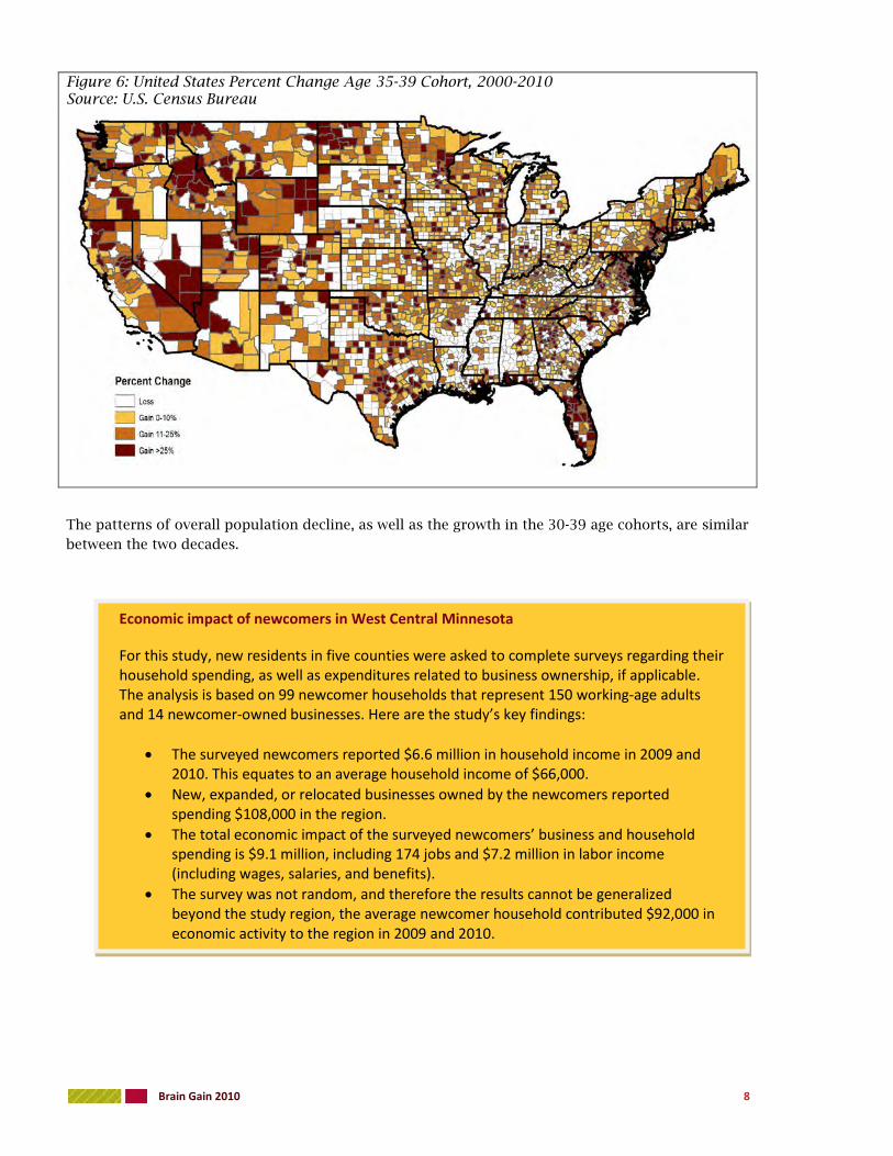
Figure 6: United States Percent Change Age 35-39 Cohort, 2000-2010 Source: U.S. Census Bureau
The patterns of overall population decline, as well as the growth in the 30-39 age cohorts, are similar between the two decades.
Economic impact of newcomers in West Central Minnesota For this study, new residents in five counties were asked to complete surveys regarding their household spending, as well as expenditures related to business ownership, if applicable. The analysis is based on 99 newcomer households that represent 150 working-age adults and 14 newcomer-owned businesses. Here are the study’s key findings:
• The surveyed newcomers reported $6.6 million in household income in 2009 and 2010. This equates to an average household income of $66,000.
• New, expanded, or relocated businesses owned by the newcomers reported spending $108,000 in the region.
• The total economic impact of the surveyed newcomers’ business and household spending is $9.1 million, including 174 jobs and $7.2 million in labor income (including wages, salaries, and benefits).
• The survey was not random, and therefore the results cannot be generalized beyond the study region, the average newcomer household contributed $92,000 in economic activity to the region in 2009 and 2010.

Brain Gain 2010 9
Minnesota cohort change Examination of Minnesota’s fluctuations show the patterns found between 1990-2000 are remarkably similar to those found in the 2000-2010 decade, both in terms of losses and gains.
Figure 7: Minnesota Population Change 2000-2010 Source: U.S. Census Bureau
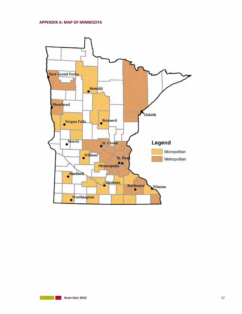
The southwestern portion of Minnesota and the western border counties experienced overall population loss (see Appendix A for a map of the state with key cities labeled). There is considerable population growth surrounding the core metropolitan counties, as well as the counties that connect Rochester to the south, and northwest to St. Cloud along Interstate 94. There is also overall growth in micropolitan counties such as Worthington and Marshall in the southwest, and in the recreational areas of north-central Minnesota.
Swift County has been, and continues to be, a challenge for describing demographic change. In the 1990s a private prison opened, which caused population growth disproportionately between 1990 and 2000. In 2010, just before the Census Bureau began work, the prison closed, and the population dropped. This skews the comparison so that Swift is not parallel to other counties.

Brain Gain 2010 10
Minnesota migration: Millennial Generation
Figure 8: Percent Population Change Age 10-19 Cohorts Source: U.S. Census Bureau
Age 10-14 Age 15-19
The migration of Millennial youth, aged 10-14 coincides, of course, with the movement of their parents. The map on the left shows widespread gains in this age group, because adults bring children to many Minnesota counties. The older part of the Millennial generation – those age 15-19 – is affected as young adults move from their hometown after graduation from high school. We see these population gains related to post-secondary school attendance in counties where there are colleges and universities – Beltrami, Clay, Stearns, Stevens, Blue Earth, Rice, St. Louis, and Winona counties.
While people may not have children at the same rate they did in the early 1900s, rural counties are destinations for those with
young children.

Brain Gain 2010 11
Minnesota migration: Generation Y
Figure 9: Percent Population Change Age 20-29 Cohorts Source: U.S. Census Bureau
Age 20-24 Age 25-29
In the past decade, just 13 (15 percent) of the 87 Minnesota counties had a net gain of Generation Y population between the age of 20 and 24. Gains in counties where colleges and universities are concentrated reinforce this finding. Even fewer counties, 11 (13 percent), experienced gains in the 25-29 age cohort. It is also interesting to see the concentrated destinations – the Twin Cities metropolitan areas and Rochester. It’s the rule that rural counties lose these young people, not the exception. We will briefly examine the extent of this loss. To do this, the following maps display percentage changes in the loss of young people. Please note the change in color gradation. Again, this special analysis describes population loss rather than gains.
Young people leave their home county. This is the rule, not the exception. College and core metro counties are their destination.

Brain Gain 2010 12
Figure 10: Percent Change Age 20-24 Cohort, Loss Categories, Minnesota, 2000-2010 Source: U.S. Census Bureau
Age 20-24 Age 25-29
Almost half of Minnesota counties, 41 (47 percent), lost more than 40 percent of their young people between the age of 20-24. Three-quarters lost more than 20 percent. Moving up to the 25-29 age cohort, 13 of the 87 counties (15 percent) lost more than 40 percent of these young people. While the number of counties experiencing this greater loss is reduced, the losses of over 20 percent are more widespread as towns with post-secondary schools begin to experience an out-migration of graduates.
Minnesota migration: Generation X
Figure 11: Percent Population Change Age 30-39 Cohorts Source: U.S. Census Bureau
Age 30-34 Age 35-39
Brain Gain 2010 13
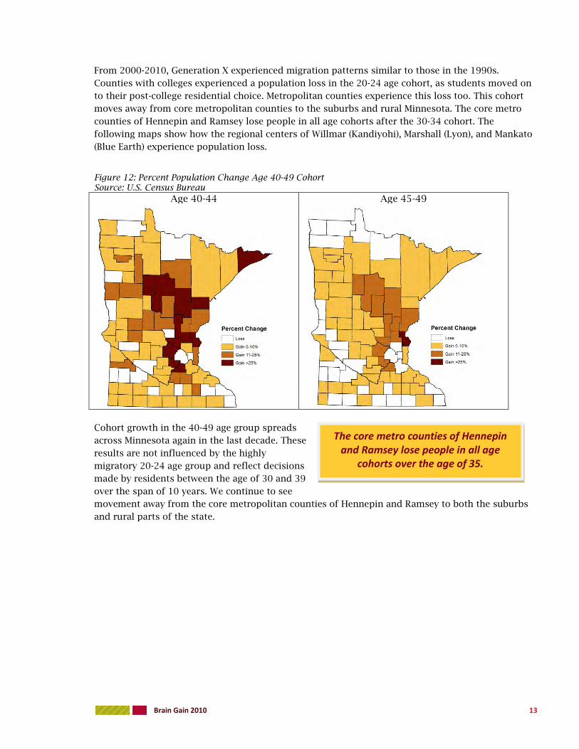
From 2000-2010, Generation X experienced migration patterns similar to those in the 1990s. Counties with colleges experienced a population loss in the 20-24 age cohort, as students moved on to their post-college residential choice. Metropolitan counties experience this loss too. This cohort moves away from core metropolitan counties to the suburbs and rural Minnesota. The core metro counties of Hennepin and Ramsey lose people in all age cohorts after the 30-34 cohort. The following maps show how the regional centers of Willmar (Kandiyohi), Marshall (Lyon), and Mankato (Blue Earth) experience population loss.
Figure 12: Percent Population Change Age 40-49 Cohort Source: U.S. Census Bureau
Age 40-44 Age 45-49
Cohort growth in the 40-49 age group spreads across Minnesota again in the last decade. These results are not influenced by the highly migratory 20-24 age group and reflect decisions made by residents between the age of 30 and 39 over the span of 10 years. We continue to see movement away from the core metropolitan counties of Hennepin and Ramsey to both the suburbs and rural parts of the state.
The core metro counties of Hennepin and Ramsey lose people in all age
cohorts over the age of 35.

Brain Gain 2010 14
Minnesota migration: Baby Boom Generation
The Baby Boom cohorts are impacted more than other cohorts by death rates that are not included in this simplified analysis (described in the methods). At the same time, this data provides fruitful information about net population flows within the state.
Figure 13: Percent Population Change Age 50-59 Cohort Source: U.S. Census Bureau
Age 50-54 Age 55-59
Figure 14: Percent Population Change Age 60-64 Cohort Source: U.S. Census Bureau
Mobilization patterns for this cohort in the first decade of the 21st century mirrored that found in the 1990s. Few counties in the southern half of the state experienced growth in these cohorts, as

Brain Gain 2010 15
Baby Boomers moved to North Central Minnesota to be closer to recreational areas during this next chapter of their lives.
SUMMARY AND DISCUSSION The 2010 update to this demographic research found the following:
The 2000-2010 migration preferences of all cohorts are remarkably similar to those found between 1990-2000;
The rural brain gain has continued in the 30-49 age range, albeit slowed;
External forces have slowed both migration rates; and,
Micropolitan counties appear to take on cohort migration traits similar to metropolitan counties.
The preference for living in small towns and rural places continues between 2000 and 2010, albeit at a slower pace. Research shows that internal migration patterns are slowing, impacting both intra-state and interstate patterns. In 2007-2008, the U.S. migration rate was found to be the lowest since World War II. This rate of 11.9 percent is down from “the 1950s, [when] almost one fifth of all Americans changed residence annually.” 7 External forces explain this decline in mobility. “Mired in housing debt and struggling through the Great Recession, more Americans are choosing to stay put rather than uproot themselves and their families,” according to the Brookings Institution
As we reflect on both the similarities and differences in data from 2000 to 2010, an additional dynamic begins to emerge. As we see in the maps, a number of rural Minnesota counties are designated as “micropolitan,” including a population of 10,000 to 49,999. It appears that there is a relationship between a micropolitan status and changes in the 30-39 cohort, primarily in the southwest portion of the state. This “rural urbanity” appears in counties that include the cities of Willmar (Kandiyohi), Marshall (Lyon), and Mankato (Blue Earth). These counties follow the core metropolitan trend of 1) attracting youth, and then 2) experiencing cohort out-migration of residents over age 30. In fact, Blue Earth County may be officially designated as urban in the next analysis by the USDA’s Economic Research Service due to be released in 2013. Ironically, this new designation might, as described earlier, exacerbate the narrative of rural decline, while increasing the “brain gain” phenomenon if the new urban space creates more longing for rural quality of life among the 30–49 age cohort.
As noted earlier, it would be wrong to paint a glowing picture of rural challenges. However, as communities and community leaders have reviewed the cohort analysis of demographic shifts, they have responded. Those who have moved to town see themselves in the research, and community leaders begin to see the benefit of attracting and welcoming newcomers. Community leaders have responded with a sense of renewed hope, by requesting, for example, additional research on the motivations of newcomers and the economic opportunity that they bring with them.
While there is no “silver bullet” in rural community development, acknowledging the reality of the brain gain allows rural places to focus on strengths and opportunities – which is the work of any community that is striving for a better future.
7 Frey, W. H. (2009, December). The great American migration slowdown: Regional and metropolitan dimensions. Washington, D. C.: Brookings Institution, Metropolitan Policy Program.

Brain Gain 2010 16
REFERENCES FOR FURTHER READING
Winchester, B. (2009, December 10). Rural migration: The brain gain of the newcomers. Retrieved from University of Minnesota Extension website: http://www.extension.umn.edu/U-Connect/components/BrainGain.pdf Winchester, B., Spanier, T., & Nash, A. (2011). The glass half full: A new view of rural Minnesota. Rural Minnesota Journal, 6, 1-30.
University of Minnesota Extension, Center for Community Vitality. (2012). Brain gain in rural Minnesota. Retrieved from www.extension.umn.edu/community/brain-gain
Brain Gain 2010 17
APPENDIX A: MAP OF MINNESOTA

Brain Gain 2010 18
APPENDIX B: COHORT POPULATION CHANGE, BY AGE (PERCENT)
AGE
10-14 15-19 20-24 25-29 30-34 35-39 40-44 45-49 50-54
Aitkin 18 -8 -43 -36.4 21 25.7 22.5 18.3 18.6
Anoka 7.7 -3.7 -25.6 -1.3 29.9 13.6 4 -1.6 -2.4
Becker 20.5 -2.7 -39.9 -25.8 31.3 24.5 12.1 6.6 10.5
Beltrami 2.1 24.4 31.7 -23 -33.9 -1.3 0.6 9.3 4.1
Benton -0.6 0 17.6 22.4 -13.8 -10.6 -1.9 1.1 -1.4
Big Stone 14.1 -12.8 -59.7 -43 21.6 10.8 2 6 -4.2
Blue Earth 3.5 94.5 205.1 -15.6 -55.7 -15.7 1 0.5 2.8
Brown 6.8 1.1 -24.9 -38.8 -24 -3.4 1.7 0.1 -1.3
Carlton 24 9.4 -27.9 -13.4 34.3 30.4 21 8.5 5.9
Carver 29.5 0.8 -35.9 1.7 83.5 68.6 34.6 11.4 5.2
Cass 21.9 -6 -46.1 -33.8 25.6 24.4 22.2 11.1 14.8
Chippewa 7 -10.6 -37 -27 8.2 2.6 3.8 -1.4 -7.4
Chisago 32.5 9.6 -28.5 1.3 67.3 52.6 34.5 27.9 19.3
Clay 16.4 56 83.9 -24.9 -33.6 21.3 10.2 2.4 -1.2
Clearwater 20 -0.9 -41.5 -37.3 16.4 16.7 11.8 7.7 3.1
Cook 8.7 -12.5 -37.9 -18.5 33.5 8.4 24.8 7.2 4
Cottonwood 9.2 -4 -44.5 -37.2 14.9 13.4 4 4 -1.4
Crow Wing 15.5 6.4 -21 -12.5 21.8 22.6 15.6 12.3 9.8
Dakota 8 -7.6 -27.3 9.1 35.9 9.4 1.9 -1.8 -3.7
Dodge 24.4 0.3 -40.7 -19.9 46.6 37.5 14 2.8 -3.3
Douglas 15.8 12.8 -17.9 -21 3 15.4 14.2 9.7 9.8
Faribault 10.8 -7.7 -47 -47.2 21.9 3.1 4.5 -3.3 -4.1
Fillmore 13.1 -9.6 -47.2 -30.7 18.9 9.1 5.9 1.4 -1.7
Freeborn -0.3 -6.1 -34.9 -28.3 0.6 -0.4 3.7 -2.8 -1.6
Goodhue 16.2 -4.5 -36.6 -26.9 27.6 13.7 8.9 4.6 -1.4
Grant 5.1 -8.8 -50.8 -28.7 16.7 12.4 8.2 3.9 1.9
Hennepin -5.3 -4.1 12.1 38.7 9.1 -16.5 -15.6 -11.6 -10
Houston 3.9 -11.9 -50 -32.5 9.8 11.4 0 -1.1 -1.1

Brain Gain 2010 19
AGE
10-14 15-19 20-24 25-29 30-34 35-39 40-44 45-49 50-54
Hubbard 21.9 4.2 -43.3 -28 27.7 31.7 25.7 24.6 12.1
Isanti 35.2 9.1 -24.7 -5.7 57.3 38.8 20.8 10.9 7.7
Itasca 22 6.2 -40.9 -38 12.4 24.4 12.7 6.9 3.7
Jackson 12.6 -6.7 -47 -39.7 9.6 2 1.7 -4 -7.9
Kanabec 18.4 -1.5 -43.6 -27.3 31.7 16.7 15.5 13.9 5.5
Kandiyohi 2 5.9 -17.2 -27.7 -6 -2.1 0.6 0.2 0.3
Kittson -3.9 -23.8 -61.3 -46.6 -1.1 -0.9 0.4 -0.9 -9.4
Koochiching 6.7 -9.2 -43.8 -40.5 5.2 6.5 -1 -1.6 -0.3
Lac qui Parle 11.2 -17.2 -61.6 -50.2 30.9 13.3 5.4 3.1 -3.2
Lake 4.1 -4.8 -38.9 -27.4 13.8 14.7 4.8 3.7 7.1
L. o.t. Woods 9.6 -23.9 -64 -46.9 8.2 1.7 3.5 -4.7 7.7
Le Sueur 26 -7 -39.3 -16.5 35.9 32.9 17.2 5.7 3.9
Lincoln -1.4 -23.1 -47.4 -36.2 20.5 5.3 -3.4 -12.8 3.8
Lyon -0.3 13.1 30.1 -20.2 -33.1 -5.7 -6.4 -1.8 -4.5
McLeod 6.7 -6.2 -35.8 -13.2 19.1 1.3 2.1 0.4 0
Mahnomen 17.8 -15 -39.9 -32.5 25.2 23.3 5.1 0.9 2.8
Marshall 12 -6.2 -56.6 -36.7 15.6 14.3 5.5 -2.5 -4.2
Martin 7.4 -9 -42.9 -33.7 20 4.5 0.6 1.4 -2.8
Meeker 12.9 -5.9 -42.2 -30.4 19.4 11.3 8.2 4.5 4
Mille Lacs 31.4 16.6 -28.3 -14.3 42.7 34 29.2 16.1 8.3
Morrison 9.2 -3.6 -37.4 -25.9 21.5 8.5 10.8 5.8 6.4
Mower 9.3 0.5 -22.1 -17.6 9.9 6.9 3.3 -3.6 -1.2
Murray 12.2 -13.1 -51.7 -41 24.7 -0.3 7.3 1 4.4
Nicollet 9.5 40.6 56.4 -26.3 -35 3.6 2.2 3 2.6
Nobles -2.3 0.1 -11.6 -11.9 8.9 2.1 0.9 -4.1 -4.2
Norman 4 -10.8 -60.7 -40.6 11.8 12.2 -3.5 1.5 -4.3
Olmsted 7.6 -2.2 -16.1 29.5 41.8 3.6 -1.9 0.5 1.1
Otter Tail 14.8 -3.4 -44.1 -36 11.3 8.1 10 9.2 4.1
Pennington 12.4 9.8 -12.3 -25.6 -4.8 9.8 1.7 5.2 -3.1
Pine 26.7 1.6 -31.1 -8.8 38.6 31.3 19.7 15 7.5
Pipestone 12.1 -4.6 -43.6 -33.1 13 13.1 1.5 1 -1.7

Brain Gain 2010 20
AGE
10-14 15-19 20-24 25-29 30-34 35-39 40-44 45-49 50-54
Polk 11.3 10 -9.2 -34.2 -14 14.5 7.9 3.3 -1.3
Pope 18.5 -13.9 -47.4 -31.5 23.2 21.4 13.4 0.9 2.8
Ramsey -11.1 1.6 19.5 11.9 -17.5 -22.4 -18.5 -13.6 -10.6
Red Lake 8.3 -10.9 -55 -33.5 34.7 -6.1 14.9 8 -3.4
Redwood 8.9 -7.9 -46.3 -36.5 7.5 2 -1 -0.3 -4.3
Renville 5.3 -14.8 -51.3 -36.2 7.6 -3.6 -0.6 -1.2 1
Rice 19.3 50.6 44.4 -34.3 -33.8 24.1 18.3 8.2 0.4
Rock 16.4 -6.4 -49.9 -35.2 25.3 15.1 4.6 2.9 -0.4
Roseau 0.7 -12.1 -57.4 -39.2 17.9 1.5 -3 -5.1 -2.4
St. Louis 1.9 23.5 29.2 -25.9 -27.2 0.1 0.9 0.4 -1.1
Scott 31.1 4.8 -24.2 40.5 141.9 72.8 30.8 12 10.5
Sherburne 35 12.6 -4.3 16.5 47.7 51.9 28.7 15.7 9.6
Sibley 7.3 -15.5 -46.6 -28.6 21.1 6 1.4 2 -1.4
Stearns 12.6 42.2 63.7 -20.2 -38 0.8 2.7 3.2 2.8
Steele 14.9 -2.7 -36.2 -12.5 18.2 11.8 9.1 1.9 -2.5
Stevens 2.1 87.1 92 -57.2 -62.1 1.2 6.1 -6.6 -10.6
Swift -7.3 -12.3 -42.7 -37.6 -19.3 -28.8 -26.5 -27.7 -21.9
Todd 18.9 2.6 -40.2 -40.9 10.1 12.8 14.3 5.4 3.2
Traverse 11.7 -15.8 -59.1 -49.4 15.2 -6 0.5 -1.5 -7.3
Wabasha 11.2 -10.5 -46.8 -33.2 16.7 14.3 8.6 0.8 0.6
Wadena 6 3.9 -41.7 -32.7 -3.5 17.1 5.6 8.3 -0.7
Waseca -0.2 -16.1 -33 -10.3 14 -7.1 -8 -10.5 -8.2
Washington 22.7 -1 -30.6 0.5 57.1 37.2 16.6 5.9 2
Watonwan -7.3 -11.7 -40.2 -34.5 1.9 1.2 -1.2 0 -6.3
Wilkin 9.1 -13.5 -52.6 -41.4 -4.3 14.4 -7.2 -1.4 -10.1
Winona 0 79.4 118.6 -42.5 -57.2 -13.3 -3 -3.1 -1.7
Wright 34.8 8.2 -30.5 16.6 105.1 64.8 32.7 16.9 10.5
Y. Medicine 12.1 -4 -40.4 -34.6 4.4 6.5 15.8 -5.7 -2.3

Brain Gain 2010 21
APPENDIX C: COHORT CHANGE MAPS, 1990-2000
Table: Percent Change Age Cohorts, Minnesota, 1990-2000 Source: U.S. Census Bureau
10-14 15-19
Table: Percent Change Age Cohorts, Minnesota, 1990-2000 Source: U.S. Census Bureau
20-24 25-29
Brain Gain 2010 22
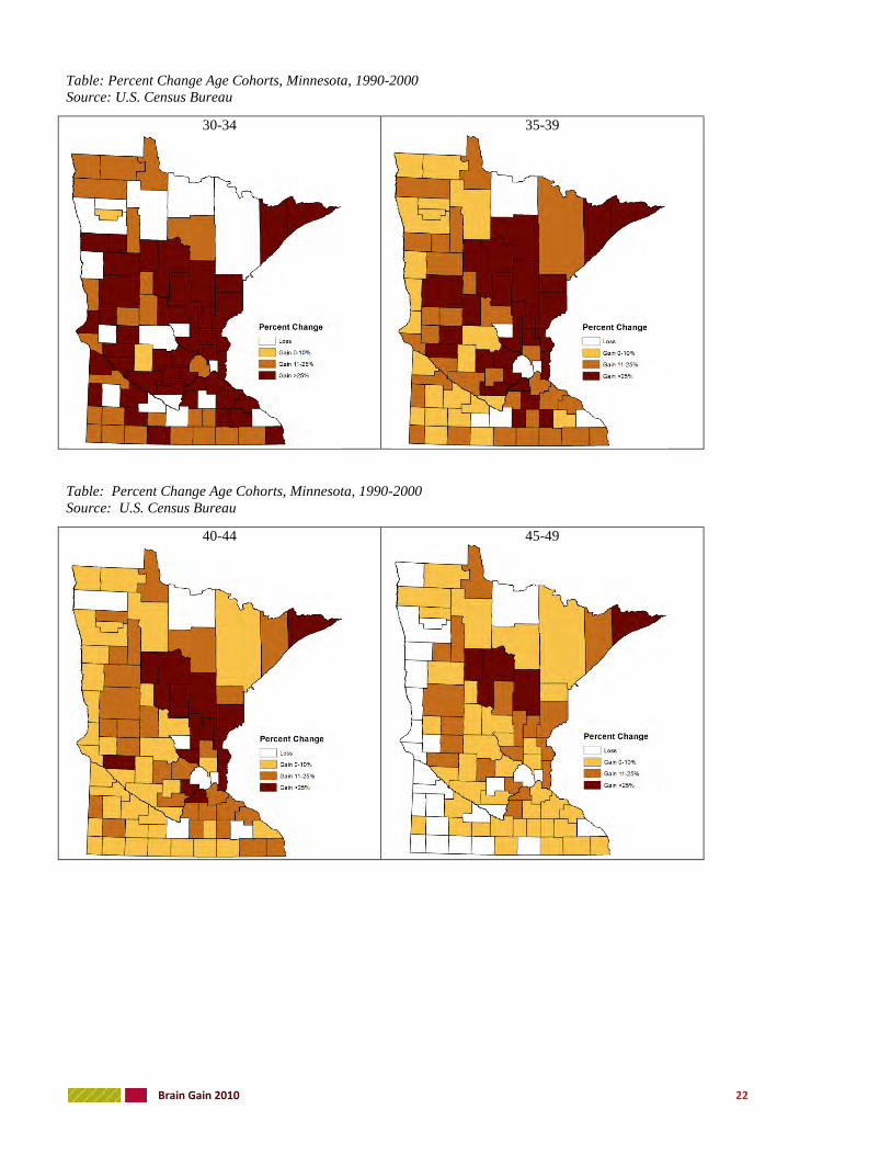
Table: Percent Change Age Cohorts, Minnesota, 1990-2000 Source: U.S. Census Bureau
30-34 35-39
Table: Percent Change Age Cohorts, Minnesota, 1990-2000 Source: U.S. Census Bureau
40-44 45-49

Brain Gain 2010 23
Table: Percent Change Age Cohorts, Minnesota, 1990-2000 Source: U.S. Census Bureau
50-54 55-59
Table: Percent Change Age Cohorts, Minnesota, 1990-2000 Source: U.S. Census Bureau
60-64