Embed Size (px)
Citation preview

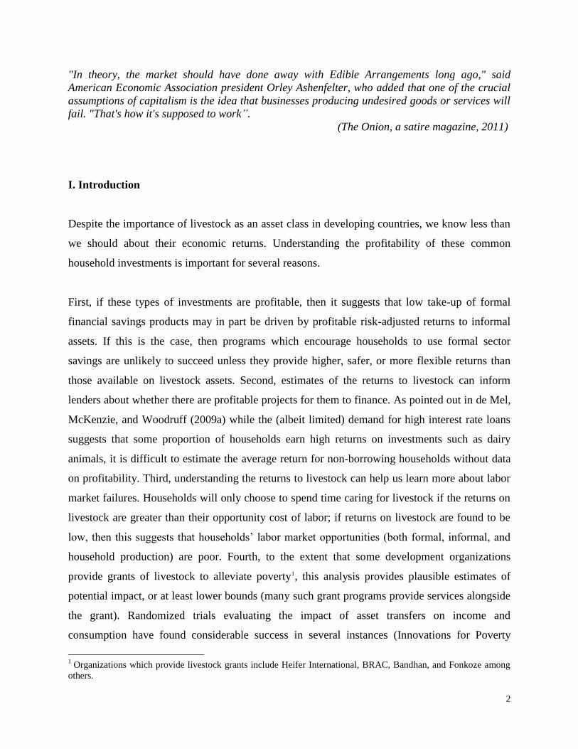
NBER WORKING PAPER SERIES
CONTINUED EXISTENCE OF COWS DISPROVES CENTRAL TENETS OF CAPITALISM?
Santosh AnagolAlvin EtangDean Karlan
Working Paper 19437http://www.nber.org/papers/w19437
NATIONAL BUREAU OF ECONOMIC RESEARCH1050 Massachusetts Avenue
Cambridge, MA 02138September 2013
The authors thank Rachel Strohm, Ellen Degnan and Joe Long for commenting on drafts of this paper,and Donghyuk Kim for research assistance. We thank the Bill and Melinda Gates Foundation for supportfor this project. All errors and opinions are our own. The views expressed herein are those of the authorsand do not necessarily reflect the views of the National Bureau of Economic Research.
NBER working papers are circulated for discussion and comment purposes. They have not been peer-reviewed or been subject to the review by the NBER Board of Directors that accompanies officialNBER publications.
© 2013 by Santosh Anagol, Alvin Etang, and Dean Karlan. All rights reserved. Short sections of text,not to exceed two paragraphs, may be quoted without explicit permission provided that full credit,including © notice, is given to the source.

Continued Existence of Cows Disproves Central Tenets of Capitalism?Santosh Anagol, Alvin Etang, and Dean KarlanNBER Working Paper No. 19437September 2013, Revised October 2013JEL No. E21,M4,O12,Q1
ABSTRACT
We examine the returns from owning cows and buffaloes in rural India. We estimate that when valuinglabor at market wages, households earn large, negative average returns from holding cows and buffaloes,at negative 64% and negative 39% respectively. This puzzle is mostly explained if we value the household’sown labor at zero (a stark assumption), in which case estimated average returns for cows is negative6% and positive 13% for buffaloes. Why do households continue to invest in livestock if economicreturns are negative, or are these estimates wrong? We discuss potential explanations, including labormarket failures, for why livestock investments may persist.
Santosh AnagolUniversity of Pennsylvania3620 Locust Walk1458 SH-DHPhiladelphia, PA [email protected]
Alvin EtangEconomic Growth CenterYale [email protected]
Dean KarlanDepartment of EconomicsYale UniversityP.O. Box 208269New Haven, CT 06520-8629and [email protected]
2
"In theory, the market should have done away with Edible Arrangements long ago," said
American Economic Association president Orley Ashenfelter, who added that one of the crucial
assumptions of capitalism is the idea that businesses producing undesired goods or services will
fail. "That's how it's supposed to work”.
(The Onion, a satire magazine, 2011)
I. Introduction
Despite the importance of livestock as an asset class in developing countries, we know less than
we should about their economic returns. Understanding the profitability of these common
household investments is important for several reasons.
First, if these types of investments are profitable, then it suggests that low take-up of formal
financial savings products may in part be driven by profitable risk-adjusted returns to informal
assets. If this is the case, then programs which encourage households to use formal sector
savings are unlikely to succeed unless they provide higher, safer, or more flexible returns than
those available on livestock assets. Second, estimates of the returns to livestock can inform
lenders about whether there are profitable projects for them to finance. As pointed out in de Mel,
McKenzie, and Woodruff (2009a) while the (albeit limited) demand for high interest rate loans
suggests that some proportion of households earn high returns on investments such as dairy
animals, it is difficult to estimate the average return for non-borrowing households without data
on profitability. Third, understanding the returns to livestock can help us learn more about labor
market failures. Households will only choose to spend time caring for livestock if the returns on
livestock are greater than their opportunity cost of labor; if returns on livestock are found to be
low, then this suggests that households’ labor market opportunities (both formal, informal, and
household production) are poor. Fourth, to the extent that some development organizations
provide grants of livestock to alleviate poverty1, this analysis provides plausible estimates of
potential impact, or at least lower bounds (many such grant programs provide services alongside
the grant). Randomized trials evaluating the impact of asset transfers on income and
consumption have found considerable success in several instances (Innovations for Poverty
1 Organizations which provide livestock grants include Heifer International, BRAC, Bandhan, and Fonkoze among
others.

3
Action 2013), but studies to date have evaluated bundled interventions which include the
provision of savings accounts, health trainings, and consumption support as well as livestock
grants, rendering it difficult to isolate the returns to livestock specifically.2
We use newly collected animal level survey data from northern India to estimate the returns to
owning dairy cows and buffaloes. We are motivated to study dairy animals in India because of
their importance as an asset among India’s rural poor. India holds more than a sixth of the
world’s population and over one quarter of the world’s estimated cattle population. The Rural
Economic and Demographic Survey (REDS), a nationally representative survey of rural India,
found that 45 percent of rural Indian households owned at least one cow or buffalo in 1999, and
on average those who have a cow or buffalo have an adult female. Our survey data provides
information on all the major inputs in the milk production function including the value of the
animal, fodder costs, veterinary costs, and lactation periods, as well as detailed data on animal
outputs including milk, calves, and dung. We estimate annual returns to owning a dairy animal
based on estimates of accounting profits (excluding the opportunity cost of labor) and economic
profits (including the opportunity cost of labor, but not including the opportunity cost of capital).
Our main finding is that, on average, households earn negative returns on their investments in
cows and buffaloes if labor is valued at market wages: we estimate average returns of negative
64% and negative 39% for cows and buffaloes respectively. If we value the household’s own
labor at zero, estimated average returns increase, to negative 6% for cows and positive 13% for
buffaloes. We conduct a variety of robustness checks to consider measurement error in the value
of inputs and outputs as an explanation for our estimated low returns. For example, we replace
self-reported values of fodder with estimated costs from a fodder production company in India
and find that estimated returns still appear to be low. We also conduct sensitivity analyses by
adjusting the data for outliers, but still find low estimated returns.
Estimates of low or negative returns present a puzzle similar to the “Edible Arrangements”
satirical quote at the opening of this paper: if cows and buffaloes earn such low, even negative,
economic returns, why would rural Indian households continue to invest in them? The second
part of our paper puts forward theories as to why households might persist in investing in cows 2 See http://www.poverty-action.org/ultrapoor/about for information on ongoing randomized trials of an integrated
intervention on asset transfers, typically livestock.
4
and buffaloes despite their low returns. While the data at hand do not allow us to distinguish
conclusively between these various explanations, we present some evidence to suggest that some
explanations appear more plausible than others.
The paper proceeds as follows. Section II describes the data and methods for calculating the
returns to cows and buffalos. Section III presents the estimates. Section IV discusses potential
explanations for why so many estimates are zero or negative, and Section V discusses further
research questions and policy implications.
II. Data and Methods
Data
The data were collected from the 2007 Uttar Pradesh Household Survey, also used in Anagol
(2010) and implemented by the Center for Financial Design at the Institute for Financial
Management and Research in Chennai. The data were collected for a sample of households in
two districts in the state of Uttar Pradesh in northern India: Lakhimpur Kheri and Sitapur.
The districts were split into two geographic regions, a smaller region called the "Ajbapur" area
and a larger region called the "non-Ajbapur area". The distinction was relevant for this survey as
Ajbapur is the location of a large sugarcane mill, and the survey collected detailed data on water
trading among sugarcane farmers. A complete list of villages in the two districts was obtained
from the Indian census of 2000, and seventy villages were randomly selected (with probability
proportional to size), including twenty from the Ajbapur area and fifty from the non-Ajbapur
area. Within each village in Ajbapur, we randomly sampled 10 households from the full village,
and an additional 20 households among all households that were identified as selling water in the
village in a household listing survey. 3 In non-Ajbapur villages we sampled 20 households
randomly from the full village and two households that were identified as jointly owning a
3 We sampled a greater number of households that traded water within the Ajbapur area because the survey was also
used to study the water trading behavior of households that lived near the sugarcane mill in Ajbapur.

5
borewell in the village. 4,5
All households in the survey, including the water-seller respondents,
were asked the same set of questions regarding their dairying behavior.
The survey asked detailed questions about livestock, farming practices, land holdings, assets,
household consumption and income history, savings, borrowing, and shocks. The “animal
details” section of the questionnaire (Section E) focused on one randomly chosen dairy animal
owned by the household, asking if the animal was a cow or buffalo and other details about the
animal.6 For an adult female dairy animal, the survey asked how many liters of milk were given
at different stages of the lactation period, including immediately after giving birth to a calf, three
months after giving birth, six months after giving birth and nine months after giving birth. The
survey also asked about the number of insemination attempts it would take to impregnate the
animal, the number and value of male and female calves born to the animal, the number of dung
cakes the animal produces per day, the number of times the animal had visited the veterinarian in
the 12 months preceding the survey, the costs associated with these visits, and the costs of
feeding the animal (including both purchased and home-produced fodder).
Estimating the Rate of Return
Our equation for the annual rate of return on a cow or buffalo is
4 Due to unsatisfactory performance by the initially hired data entry firm, we switched data entry firms and re-
entered all of the data. In the process of transferring the hard copies of surveys from the first data entry firm to the
second, 11 percent of the original surveys were lost. Among the non-Ajbapur villages, we received 967 of the
expected 1100 surveys. Three villages in the original non-Ajbapur sample frame were lost. Among the Ajbapur
villages, we received 546 of the expected 585 surveys. We received surveys from all of the villages that were
originally included in the Ajbapur sample frame. Overall, we are missing data from eleven percent of households in
the original sample frame. 5 The survey collected a larger number of observations from water sellers in the Ajbapur to study water trading
amongst those living close to a sugarcane mill. In the non-Ajbapur area, the survey collected information on two
households that jointly owned borewells as baseline information for a potential field experiment on joint ownership
of borewells. 6 The dairy section of the questionnaire (Section D) asked if the household owned any female cows/buffaloes; if so,
how many cows/buffaloes the household owned. For each cow or buffalo owned, households were asked to record,
beginning with the most valuable cow/buffalo and then proceeding in order of declining value, the animal’s breed,
and what its selling price would be if the household wanted to sell the animal. The enumerator was then instructed to
administer the detailed animal questions (Section E) regarding the animal in this list whose ID number appeared first
on a sticker (unique to each survey) which contained a randomized ordering of all the Animal IDs.

6
where is the price at end of year, is the price at the beginning of the year, and is
the profit generated by the animal over the year. We estimate the term as the average
change in the value of animals that go from the animal’s current age in our data to their current
age plus one year. We estimate the flow profits ( ) as the revenues from milk, calves and
dung minus fodder, veterinary, and insemination costs.
The first calculation we need to perform to estimate the annual return to a dairy animal is how
many lactations, on average, the typical animal has per year. Our survey asked households how
many calves they expected the sampled dairy animal to have in the rest of its life (having a calf is
a necessary and sufficient condition for having a lactation). We take this number and divide it by
an estimate of the number of years we expect the sampled animal to live.7 For cows, the average
number of calves expected per year is 0.89, and for buffaloes the average number of calves
expected per year is 0.97. For simplicity, we assume that cows and buffaloes in our sample will
produce one calf, and thus have one lactation period, per year.8
The annual input and output variables used in the calculations are as follows.
Inputs
1. Fodder costs: Dairy animals typically eat more during the time when they are giving milk
versus the time when they are dry. For each cow or buffalo in our survey, we have separate
estimates for the cost of feeding the animal when it is milking versus dry. We combine this
information with previous estimates on the average amount of time Indian dairy animals
spend dry versus milking per year. Dry periods for cows and buffaloes in India are estimated
to be approximately 160 days per year (Anagol 2010). Since we are estimating returns over a
one-year period, assuming a 365-day year implies that milking periods are 205 days per year
7 We estimate a dairy’s animals expected years to live as follows. We first take the observed age distribution of cows
above the age of six years old in our sample, and estimate the probability of death at each age based on the
proportionate decrease in the number of cows at each age level. We also assume that cows or buffaloes that reach
the age of 15 will die in that year, as this is the oldest observed animal we see in our data. Using this estimate of a
mortality table for cows, we can estimate an animal’s expected to years to live conditional on obtaining its current
age. For animals less than six years of age, we assume that they will make it to age six with probability one. We
make this assumption as our data contains few observations of animals less than six years old so our estimated
mortality table is not accurate for the younger ages. 8 The assumption of one calf per year is likely an over-estimate, as even dairy cows in the US typically do not birth
more than one calf per year on average.
7
(roughly seven months). The survey asked how many months the animal will give milk after
it gives birth. The average response was seven months (but can go up to 10 months for some
animals), which is consistent with the estimated 205 days we use to estimate annual fodder
costs. To validate the fodder costs reported by our respondents, we also conduct a robustness
test using a different measure of fodder costs developed by the Kisan Fodder Company, a
livestock enterprise based in Uttar Pradesh. Kisan provides an estimate of the amount of
fodder necessary for an animal to eat to produce a certain amount of milk.9 We combine their
estimates with our data on the amount of milk the animal gives per lactation to estimate the
cost of feeding the animal during the year.
2. Appreciation and depreciation of dairy animal value: Consider an animal in our sample that
was three years old at the time of our survey. To estimate the change in the value of this
capital asset (i.e. ) we assume that this animal’s value will change, on average, the
same as the difference in value of all four-year-old animals and all three-year-old animals in
our sample.
3. Veterinary costs (costs of examinations and procedures during visits to a veterinarian): We
have a direct survey question that asks how much the household spent on veterinary costs for
the animal over the past year.
4. Cost of insemination: This is determined by the number of insemination attempts needed to
impregnate the animal multiplied by the cost for one insemination. 78 percent of animals
where we collected detailed information were inseminated using a breeding bull, and 13
percent were inseminated using artificial insemination, and 9 percent were inseminated using
both methods (the households tried different methods). The survey did not include a direct
question on the cost of using natural insemination, so we make the conservative assumption
that natural insemination is as expensive as artificial insemination.10
Insemination services
are typically provided by either a government veterinary hospital or an NGO in our survey
villages. Our village level survey suggests that the average cost of one insemination by a
government hospital was 66 rupees. For an NGO, the corresponding figure was 70 rupees. As
we are unable to distinguish between the services provided by the two providers, we assume
9 The exact mapping that Kisan Fodder uses between milk production and fodder consumption is described in the
Appendix to this paper. 10
In reality we suspect that natural insemination is cheaper than artificial insemination, as local bulls are typically
maintained in villages for insemination purposes. Nonetheless, given the low price of insemination in general it is
unlikely our results are driven by measurement error in insemination costs.

8
the price is the average of the two, 68 rupees. Sensitivity analysis shows that the results are
unchanged regardless of whether a price of 66, 68 or 70 rupees is used.
5. Labor costs: Our survey asked about the number of hours spent caring for animals per day in
the household where the sampled animal lives. We estimate the cost per hour of this labor as
follows. We observe that children and adults (both men and women) in the household are
generally equally responsible for the care of the animal.11
According to our village level
survey, the daily wage rate for an adult (man or woman) is 60 rupees, and the child labor
wage rate per day is 25 rupees. In our baseline estimates we thus assume that the cost of
taking care of the dairy animal is 42.5 rupees per day. Assuming an eight hour work day, this
gives an hourly labor cost of approximately 5 rupees. 12 The average number of hours spent to
tend the animal is 3.5 hours (with a standard deviation of 1.06), with the 25th percentile
being 3 hours and the 75th percentile 4 hours. An important point to note is the possibility of
multi-tasking when tending the animal. It is possible that the animal is taken out to pasture
while the caretaker is doing something else (for example, working on the farm, doing
something in the neighboring plot, etc.). Our survey did not ask any direct questions about
multi-tasking so we cannot directly assess its importance. We account for the fact that multi-
tasking might reduce the effective cost of labor by including return calculations where we
assume the value of labor is zero (our “accounting” rates of return).
Outputs
1. Value of milk: Our survey asked the following questions to determine the value of milk
produced by the animal per lactation. We asked for the number of liters of milk produced
during the first three months after birth, from three to six months, from six to nine
months, and from nine to ten months. We asked for potentially differing amounts of milk
production based on months since birthing, as cows and buffaloes typically give the most
milk around four to five months after giving birth and then reduce milk production as the
calf switches to solid foods. We multiply the liters per day estimate by the household’s
11 We do not know which household members take care of these particular animals. However, the survey asks
whether a household has owned any female cows or buffaloes in the past five years and which members of this
household are responsible for dairy animals. According to the data, it is common practice for household members
(adult males and females as well as children) to share the responsibility of taking care of their cows and buffaloes. 12
According to The Times of India (2011), the average for the OECD nations is 8 hours a day, slightly below the
figure for Indians at 8.1 hours (486 minutes). Accessed online at http://articles.timesofindia.indiatimes.com/2011-
04-13/india-business/29413474_1_oecd-countries-cooking-indians-work

9
response to a survey question on the average price of milk produced by the household.13
The value of milk produced by the cow/buffalo when it is dry is assumed to be zero.
2. Value of calves: Given that we estimate dairy cows and buffaloes have approximately one
lactation per year, this implies that they would produce one calf per year (on average).
For each cow and buffalo in our sample, the survey asked the respondent to estimate what
a new calf of this particular animal would be worth (separately for male and female
calves) at the time of birth. Given that male and female calves are equally likely to be
born, we take the average value of male and female calves as the expected value of a calf
during its first year.
3. Value of dung cakes14: Our survey asked the respondent to estimate the number of dung
cakes the animal produces per day. We combine this information with the estimated value
of a dung cake as provided in the village survey (1 rupee per dung cake), to estimate the
value of dung cakes produced per year.
4. Value of adult animal: Our survey asked what the value of the animal would be if the
animal were sold in the near future. This is the value we use to estimate .
III. Estimates
The sample includes 300 cows and 384 buffaloes. Table 1 presents summary statistics of the
sources of value and expenditure. Right after giving birth to a calf, a buffalo produces three and a
half liters of milk per day, on average, and a cow produces three liters of milk per day, on
average. Between three to six months after giving birth, the quantity of milk produced increases
by half a liter for buffaloes and one-quarter of a liter for cows. Milk yield then declines between
six to nine months after giving birth: buffaloes give three liters per day, and cows two liters per
day. After this period, the animals get closer to becoming completely dry, with buffaloes
yielding one liter per day and cows one-half of a liter per day. The trend in milk yield over the
13
The survey did not ask for specific price per liter estimates for each animal in the household as fieldwork during
piloting suggested there was not substantial variation in the price per liter of milk within households. 14
Cow dung can be used in several ways. First, dung cakes are a source of domestic fuel in many rural households
in India (Aggarwal and Singh 1984). Second, dung is often used as agricultural fertilizer (Aggarwal and Singh
1984). Third, due to its insect repellent properties for some types of insects (such as mosquitoes), dung is used to
line the floor and walls of buildings (Mandavgane, Pattalwar, and Kalambe 2005). Dung is therefore important,
allowing households to save money that would otherwise be spent on alternatives such as firewood, fertilizer and
insecticides.

10
lactation is illustrated in a bar chart shown in Figure 1 and the distribution of milk produced per
day is shown in Figure 2.
Table 1 shows that there are no differences between cows and buffaloes with regard to the
remaining inputs: labor hours, veterinary expenses, and insemination expenses. A typical animal
visits the veterinarian once per year. Four labor hours are spent each day tending the animal; and
it takes two insemination attempts to get it pregnant during a 12-month cycle. On average, the
animal produces four units of dung cakes per day.
Our estimates of the accounting profits to owning a cow or buffalo (i.e., labor valued at zero) are
presented in Table 2a-d. In Table 2a the top row shows the mean values of inputs and outputs,
total costs, profits, and rates of return for the cows whose rates of return fall within the top
twenty percent of rates of return overall; the next row shows the mean values of inputs and
outputs for cows whose rates of return fall between the 20th
and 40th
percentile. The second panel
shows the same calculations for our sample of buffaloes.
The results in Tables 2a show negative accounting profits (-6%) for cows, and positive profits
(13%) for buffaloes. A Mann-Whitney test indicates that the difference between the two means is
statistically significant at 1%. The tables also show the distribution of returns for both cow and
buffaloes. There is substantial variation in the calculated rates of return across our groups, and
thus it is important to determine to what extent our mean estimates of rates of return are
influenced by outliers.
The quintile based mean estimates show that the adult value of animals (Column C) and value of
fodder costs (Column F) have the most substantial amount of variation across the quintiles and
therefore may be driving a lot of the variation in rates of return. We now evaluate how sensitive
our mean estimates of rates of return are to outliers in the adult value of animals and fodder
costs.
Table 2b presents estimates of the accounting returns to owning cows and buffaloes assuming all
cows/buffaloes had an adult value equal to the median adult value in the data. Replacing a cow’s/
buffalo’s survey-based adult value with the median value in the data mechanically removes any
outliers on adult values. The results remain similar for cows (the rate of return is -9% on
average), but higher returns are obtained for buffaloes (about 20% on average).
11
Table 2c examines the sensitivity of our mean estimate of returns to fodder costs. This table is
the same as Table 2a, except now for each animal we replace the household’s estimate of fodder
costs with our estimate of the animal’s fodder cost based on the amounts of fodder recommended
by the Kisan fodder company. Given that the Kisan fodder company uses a simple linear formula
for fodder based on the liters of milk an animal gives, this will mechanically remove any major
outliers in the household’s estimates of fodder costs. We find that, overall, cows earn an average
rate of return of 15% per year and buffaloes earn an average return of 5% per year.
Table 2d reports our estimates after both adjusting for outliers in the mean values of animals (as
in Table 2b) as well as adjusting for outliers in fodder costs (as in Table 2c). After removing
these outliers, we find that cows have an average return of 21% per year and buffaloes have an
average return of 7% per year.
The annual interest rate paid to saving accounts by many formal banks in India ranges between
4-10%. As another point of comparison, the nominal yield on ten-year Indian government bonds
in 2007 (the year of our survey) was 8.5% (Campbell, Ramadorai, and Ranish 2012). Accounting
profits from the Kisan calculation suggest that the rate of return from cows and buffaloes are not
substantially higher than these low risk financial assets. For cows our return estimates range
from -9% to %21, and for buffaloes our estimates range from -38 percent to 20 percent. While
both of these ranges include returns that are higher than formal savings products, it is important
to note that these ranges are calculated before we include the cost of any labor spent on caring
for animals or adjust for the fact that livestock investments are likely more risky than formal
financial products (livestock can get sick, die or have problems getting pregnant). Given that
labor costs and animal risk are likely to reduce the real returns experienced by households, we
argue that it is unlikely that livestock investments offer better returns than formal savings
products.
In Tables 3a, 3b, 3c, and 3d we explore the possible impact of labor costs on the estimated
returns to Indian dairy animals. As expected, including labor costs drives all of our return
estimates to be negative, with the average return to a cow equal to -64% and to a buffalo equal to
-39% when calculated with self-reported fodder costs and using the mean animal values (Table
3a). These large and negative results remain when we adjust for outliers in animal values (Table
3b), adjust for outliers in fodder costs (Table 3c), and when we adjust for both outliers in animal

12
values and fodder costs (Table 3d). While we do not have panel data to allow us to estimate the
impact of animal risk on returns, we believe that incorporating animal risk in to our return
estimates would also lead to low returns relative to formal savings products. Overall, these
results raise an important question: if these estimates are correct and cows and buffaloes are not
economically profitable, why do households hold onto these animals instead of selling them?
IV. Potential Explanations
1. Measurement Error
The first explanation of our finding is the simplest: our data or assumptions on production of
cows are wrong. Our estimates ultimately rely on household self-reports on the costs and
revenues of dairy animal production, and so if households misstate revenues or costs our findings
of low returns might not reflect true returns. Indeed, in Sri Lanka, de Mel, McKenzie, and
Woodruff (2009a) find that firms systematically under-report revenues by about 30% and over-
report costs. They conclude that simply asking firms how much profit they make provides a more
accurate measure of profits than detailed questions on revenues and expenses.
Previous work in labor economics has found that workers in formal employment settings
typically do over-state the amount of hours worked (Bound et al. 1994; Carstensen and Woltman
1979; Duncan and Hill 1985; Hamermesh 1990; Mellow and Sider 1983; Robinson and Bostrom
1994; Stafford and Duncan 1977). Nonetheless, the fact that we find modest average returns even
when we assume that labor costs are zero suggest that over-stating the amount of time spent on
dairying is not the sole driver for our low estimated returns.
2. Preference for Home -Produced Milk
Anecdotal evidence suggests that Indian households believe, and perhaps rightly so, that home
produced milk is of higher quality than purchased milk. Reuters (2012) recently reported that
much of the country’s milk is either diluted or contaminated with chemicals, including bleach,
fertilizer or detergents. A government survey also found that 68.4% of milk sold in India does
not meet basic health standards (FSSAI 2011). This implies that households may value home-
produced milk at a rate higher than the market value, and therefore may be willing to receive low
financial returns on dairy investments in exchange for the guarantee of having high quality milk
available for household consumption. Consistent with this hypothesis, we find that only 12% of

13
our sample households actually sold milk in the past year.15
If the value of self-produced milk
was 20% higher than the market price, the average accounting return to cows would rise from
negative 6% to a positive 10%.16
3. Preference for Illiquid Savings
In developing countries, low-income individuals and small businesses are generally excluded
from conventional financial institutions (Rutherford 2000). de Mel, McKenzie, and Woodruff
(2009b) document that few poor households have formal savings accounts. However, as
Rutherford (2000) emphasizes, low income households do typically have some savings. This has
led to the proliferation of a variety of forms of semiformal or informal savings channels,
including deposit collectors,17 savings clubs, postal accounts, accumulating savings and credit
associations (ASCAs), rotating savings and credit associations (ROSCAs), or saving at home.
These savings channels may help to meet the needs of the poor by offering convenient services
in their neighborhoods (as in the case of deposit collectors), allowing them access to loans
(ASCAs and ROSCAs), and providing them with incentives to save (in the form of the social
pressure present in savings clubs, ROSCAs and ASCAs).
However, there are also disadvantages associated with these types of informal savings. The use
of deposit collectors entails a negative interest rate. Interpersonal conflict or lack of trust may
inhibit the creation of savings clubs, ROSCAs and ASCAs, and keeping money in the home
offers no shield against inflation, and may lead to temptation spending. In the face of these
shortcomings, households may find it desirable to save a portion of their income close to home in
illiquid assets such as livestock, even if the returns to this means of saving are low, or even
negative.
4. Labor Market Failures: True Value of Marginal Time is Zero
15
There are other potential explanations for why so few households sell milk. Another plausible explanation is that
there is limited external demand for the milk produced in our sample villages; only 23% of our sample villages are
visited by milk buyers, and only 8% have a milk cooperative. 16
If further evidence showed that households primarily hold low return cows as a way to guarantee clean milk
supply, then inspection policies or business innovations (i.e., quality verification markets) that reveal the hidden
information in milk markets could be welfare enhancing. 17
In West Africa susu (deposit) collectors are paid up to 40% interest for providing a means of saving for rural
households (Rutherford, 2000).

14
If labor markets are missing or imperfect, particularly for women18, then the true opportunity cost
of labor may actually be zero or close to zero (Basu 1997; Dasgupta 1993; Bardhan 1984;
Mammen and Paxson 2000). In many locations, the formal labor market for women is essentially
non-existent (Emran and Stiglitz 2006). Mammen and Paxson (2000) note that “there may be
costs associated with women working outside of the domain of the family farm or non-farm
family enterprise. Custom and social norms may also limit the ability of women to accept paid
employment, especially in manual jobs. Further, off-farm jobs may be less compatible with child
rearing, creating fixed costs of working off-farm” (p. 143). This implies that the household
optimization treats the female labor endowment as effectively non-traded. One would expect that
as the costs of women’s time increases as they enter the workforce, the opportunity cost of
tending a cow would also rise. However, if there are no opportunities for people to enter the
workforce, then the opportunity cost of raising an animal is effectively zero, or at best the value
of other home production opportunities.19
5. Preference for Positive Skewness in Returns
Garrett and Sobel (1999) document theoretical and empirical evidence that positive skewness of
prize distributions explains why risk averse individuals may play the lottery. Similarly, skewness
of returns distributions may explain why people may hold female cows and buffaloes, given that
there is a small probability of making huge profits, although on average the animals yield
negative economic returns. Our estimates provide evidence for positive skewness in returns. For
example, Table 2a shows that the top 20% cows and buffaloes generated huge profits of 378%
and 322%, respectively. At the same time, the bottom 40% of cows and buffaloes make
substantial losses. This is consistent with the model of learning and types of enterprise presented
in Karlan, Knight, and Udry (2012), which predicts that a majority of entrepreneurs will have
low marginal returns to capital as they are not capable of running a larger business, but that a
small proportion of entrepreneurs may have the skills to run large firms profitably.
6. Social and Religious Value
18
For about half the households analyzed, women are responsible for tending the animals. 19
Based on the traditional assumption made in the literature that the value of an individual's time spent in any
activity is equal to his or her wage rate.

15
In Hinduism, the cow is a symbol of wealth, strength, abundance, selfless giving and a full
earthly life.20 As almost all the sampled households reported that they were Hindu, they may also
derive spiritual returns from cattle ownership. The foregone returns compared to their next best
investment alternative would effectively be the cost of religiosity in this context. This of course
does not explain the results for buffaloes. It also requires believing that the long term social
evolution of a religion could find an equilibrium in which individuals worship a loss-inducing
investment; most economic models of religion predict that customs derived from religion are
either beneficial or strengthen the group, and this seems to do neither (Bainbridge and
Iannaccone 2010).
V. Further Research Questions and Policy Implications
Our goal here is not to determine conclusively why Indian households invest in cows and
buffaloes despite the fact that economic returns to such investments seem to be frequently
negative. Our goal, rather, is put forward a puzzle, with the aim to motivate either better data, or
better understanding of these markets or behavioral decisions, in order to explain the puzzle.
With a better understanding of the driving market or behavioral failures, if any, one can then
focus policies on specific market problems.
Evidence suggests that the poor are often willing to earn negative interest in order to access
reliable saving services (see Dupas and Robinson (2012) for evidence on savings accounts with
negative interest rates in Kenya and Rutherford (2000) for deposit collectors in west Africa). If
livestock ownership is seen as a form of savings, the observed negative returns to cows and
buffalo provide additional evidence of the high demand for savings, and perhaps specifically for
illiquid savings in order to avoid temptation spending. The question then turns to the supply side
of savings: what are the constraints on the supply side that make cows and buffalos better
savings alternatives than what banks offer? With technological innovations such as mobile
money, the transaction costs are plummeting for offering deposit accounts to consumers in
developing countries, even in highly rural areas. Thus this is an area where improvements in
ability to store cash outside of the home may lead to more efficient allocation of capital, away
from risky or low return home investments. If the introduction of high quality savings accounts
20
For a general review of the debate on why cows evolved to become holy in Hinduism see Korom (2000).

16
leads to a reduction in cow and buffalo ownership, this would be evidence for the commitment to
save explanations discussed above.
If indeed, as we find, owning cows yields low or negative returns, this is of critical importance
for NGO and government programs that promote investment in cows with an aim of poverty
alleviation. In particular, the results here are critical for programs that engage in livestock grants
to help households start or expand income generating activity from raising livestock (this is
common amongst “graduation” programs, cited earlier, as well as many NGOs, such as Heifer
International or other livestock grant programs). Our results suggest that merely transferring an
asset alone may not be sufficient to generate higher income (beyond the value of the transferred
asset). The heterogeneity in returns we observe may of course be due to heterogeneity in skills
and knowledge on how to raise dairy animals profitably; this suggests potential for training and
monitoring to improve the returns for households.
Our results are also consistent with the finding in de Mel, McKenzie, and Woodruff (2009b) that
female owned enterprises in Sri Lanka have a marginal return to capital equal to zero.
Fafchamps et al. (2011) also find that the returns to capital are equal to zero for female
enterprises with less than the median level of profits prior to the capital infusion. Given that in
our context the maintenance of dairy animals is managed by the women and children of the
household, a similar mechanism or failure may drive the results in both our analysis and that of
de Mel, McKenzie, and Woodruff (2009b) and Fafchamps et al. (2011)
Looking beyond cattle ownership, future research should analyze the returns from other assets,
such as trees, tubers and small livestock (Undurragaa et al. 2013). Anecdotal evidence suggests
that a variety of low-performing assets are commonly held across the developing world, but
more systematic analysis across countries and asset types, and with a focus on unpacking the
mechanisms driving ownership and returns of such assets, would further our understanding of
household finance for the poor.

17
References
Aggarwal, G.C., and N.T. Singh. 1984. “Energy and Economic Returns from Cattle Dung as Manure and Fuel.” Energy 9 (1) (January): 87–90. doi:10.1016/0360-5442(84)90079-3.
Anagol, Santosh. 2010. “Adverse Selection in Asset Markets: Theory and Evidence from the Indian Market for Cows”. Working Paper. University of Pennsylvania Wharton School.
Bainbridge, William Sims, and Laurence R Iannaccone. 2010. “Economics of Religion.” In The Routledge Companion to the Study of Religion, 2nd ed., 461–475.
Bardhan, Pranab K. 1984. Land, Labor, and Rural Poverty: Essays in Development Economics. Columbia University Press.
Basu, Kaushik. 1997. Analytical Development Economics: The Less Developed Economy Revisited. MIT Press.
Bound, John, Charles Brown, Greg J. Duncan, and Willard L. Rodgers. 1994. “Evidence on the Validity of Cross-Sectional and Longitudinal Labor Market Data.” Journal of Labor Economics 12 (3) (July 1): 345–368. doi:10.2307/2535220.
Campbell, John Y., Tarun Ramadorai, and Benjamin Ranish. 2012. “How Do Regulators Influence Mortgage Risk: Evidence from an Emerging Market”. Working Paper 18394. National Bureau of Economic Research. http://www.nber.org/papers/w18394.
Carstensen, L, and H Woltman. 1979. “Comparing Earning Data from the CPS and Employer’s Records.” In Proceedings of the Social Statistics Section, 168–173.
Dasgupta, Partha. 1993. “An Inquiry Into Well-being and Destitution”. Clarendon Press. De Mel, Suresh, David J. McKenzie, and Christopher Woodruff. 2009a. “Measuring Microenterprise
Profits: Must We Ask How the Sausage Is Made?” Journal of Development Economics 88 (1) (January): 19–31. doi:10.1016/j.jdeveco.2008.01.007.
De Mel, Suresh, David McKenzie, and Christopher Woodruff. 2009b. “Are Women More Credit Constrained? Experimental Evidence on Gender and Microenterprise Returns.” American Economic Journal: Applied Economics 1 (3) (July): 1–32.
Duncan, Greg J., and Daniel H. Hill. 1985. “An Investigation of the Extent and Consequences of Measurement Error in Labor-Economic Survey Data.” Journal of Labor Economics 3 (4) (October 1): 508–532. doi:10.2307/2534924.
Dupas, Pascaline, and Jonathan Robinson. 2012. “Savings Constraints and Microenterprise Development: Evidence from a Field Experiment in Kenya.” AEJ: Applied Economics forthcoming.
Emran, S., and J. Stiglitz. 2006. “Microfinance and Missing Markets.” Working Paper. July. Fafchamps, Marcel, David McKenzie, Simon Quinn, and Christopher Woodruff. 2011. “Female
Microenterprises and the Flypaper Effect: Evidence from a Randomized Experiment in Ghana”. World Bank.
Garrett, Thomas A, and Russell S Sobel. 1999. “Gamblers Favor Skewness, Not Risk: Further Evidence from United States’ Lottery Games.” Economics Letters 63 (1) (April): 85–90. doi:10.1016/S0165-1765(99)00012-9.
Hamermesh, Daniel S. 1990. “Shirking or Productive Schmoozing: Wages and the Allocation of Time at Work”. Working Paper 2800. National Bureau of Economic Research. http://www.nber.org/papers/w2800.
“Indians Work 8.1 Hours a Day, More Than Many Westerners.” 2011. The Times Of India, April 13. http://articles.timesofindia.indiatimes.com/2011-04-13/india-business/29413474_1_oecd-countries-cooking-indians-work.
Innovations for Poverty Action. 2013. “Impact of the Ultra Poor Graduation Model: Preliminary Results from Randomized Evaluations of Four Pilots.”

18
Karlan, Dean, Ryan Knight, and Christopher Udry. 2012. “Hoping to Win, Expected to Lose: Theory and Lessons on Micro Enterprise Development.” National Bureau of Economic Research Working Paper w18325.
Korom, Frank J. 2000. “Holy Cow! The Apotheosis of Zebu, or Why the Cow Is Sacred in Hinduism.” Asian Folklore Studies 59 (2): 181. doi:10.2307/1178915.
Mammen, Kristin, and Christina Paxson. 2000. “Women’s Work and Economic Development.” Journal of Economic Perspectives 14 (4): 141–164.
Mandavgane, S A, V V Pattalwar, and A R Kalambe. 2005. “Development of Cow Dung Based Herbal Mosquito Repellent.” Natural Product Radiance 4 (4) (August): 270–272.
Mellow, Wesley, and Hal Sider. 1983. “Accuracy of Response in Labor Market Surveys: Evidence and Implications.” Journal of Labor Economics 1 (4) (October 1): 331–344. doi:10.2307/2534858.
“Most Milk in India Contaminated or Diluted.” 2012. Reuters, January 10. http://www.reuters.com/article/2012/01/10/us-india-milk-idUSTRE80919O20120110.
Robinson, J, and A Bostrom. 1994. “The Overestimated Workweed? What Time-Diary Measures Suggest.” The Monthly Labor Review 117: 11–23.
Rutherford, Stuart. 2000. The Poor and Their Money. New Delhi: Oxford University Press. Stafford, Frank, and Greg Duncan. 1977. “The Use of Time and Technology by Households in the United
States.” http://www.eric.ed.gov/ERICWebPortal/detail?accno=ED146311. “The National Survey on Milk Adulteration.” 2011. Food Safety and Standards Authority of India. Undurragaa, Eduardo, Ariela Zychermanb, Julie Yiua, TAPS Bolivia Study Team, and Ricardo Godoy. 2013.
“Savings Before the Arrival of Markets: Evidence from Forager-farmers in the Bolivian Amazon.” Tsimane’ Amazonian Panel Study Working Paper 81.

19
Table 1 – Summary Statistics
Mean (Standard deviation)
Buffaloes
(N=384)
Cows
(N=300)
Average liters of milk per day: 0-3
months after giving birth
3.57
(1.27)
2.86
(1.23)
Average liters of milk per day: 3-6
months after giving birth
4.09
(1.41)
3.26
(1.39)
Average liters of milk per day: 6-9
months after giving birth
2.95
(1.21)
2.22
(1.07)
Average liters of milk per day: 9-10
months after giving birth
0.85
(1.06)
0.46
(0.82)
Average liters of milk per day for the
whole lactation period
3.27
(0.98)
2.54
(0.98)
Average units of dung cakes produced
per day
4.98
(2.02)
4.19
(1.80)
Average labor hours per day 3.55
(1.06)
3.52
(1.05)
Average insemination attempts per year 1.52
(1.43)
1.57
(1.42)
Average number of times the animal
visits the Veterinarian per year
0.90
(1.02)
0.82
(0.92)

20
Table 2a – Accounting Profits:
(Mean values for all variables)
Milk
Value
A
Calf
Value
B
Value of
adult
animal at
end of
year
C
Dung
Value
D
Total
Revenue
E =
A+B+D
Fodder
Cost
F
Veterinary
Cost
G
Insem-
ination
Cost
H
Total
Cost
J =
F+G+H
Change in
value of
animal
K
Profits
L = E-J
Value of
adult
animal at
beginning
of year
M=C-K
Rate of
Return
(%)
N =
(K+L)/M
Cows
Top 20% 9050 1085 3235 1570 11705 6033 135 76 6243 1414 5462 1821 377.61
Top 40% 8935 1036 6314 1527 11498 6812 128 91 7031 1071 4467 5243 105.61
Middle 20% 7500 1018 17665 1655 10172 10240 237 120 10597 742 -425 16923 1.87
Bottom 40% 6428 898 8004 1466 8792 14319 105 115 14540 -1452 -5748 9455 -76.14
Bottom 20% 6330 813 4542 1460 8603 16460 107 113 16680 -2159 -8078 6701 -152.76
All 7645 977 9260 1528 10150 10500 141 107 10748 -4 -597 9264 -6.49
Buffaloes
Top 20% 10930 1284 2361 1887 14102 5180 215 94 5489 -239 8613 2600 322.09
Top 40% 10718 1274 4423 1930 13921 5932 190 103 6225 -119 7696 4542 166.82
Middle 20% 10011 1114 15328 1782 12907 8152 111 98 8360 -287 4547 15615 27.28
Bottom 40% 8797 1225 13817 1728 11750 18310 177 106 18593 565 -6843 13252 -47.37
Bottom 20% 8199 1166 9958 1723 11088 23223 208 114 23546 899 -12458 9059 -127.60
All 9802 1222 10373 1819 12844 11368 169 103 11640 124 1204 10249 12.96
Notes: Each row presents the average value of the variable given in the Column for a given rate of return quintile. All values are Indian rupees.

21
Table 2b – Accounting Profits: (Mean values, except adult value fixed at the median)
Milk
Value
A
Calf
Value
B
Value of
adult
animal at
end of
year
C
Dung
Value
D
Total
Revenue
E =
A+B+D
Fodder
Cost
F
Veterinary
Cost
G
Insem-
ination
Cost
H
Total
Cost
J =
F+G+H
Change in
value of
animal
K
Profits
L = E-J
Value of
adult
animal at
beginning
of year
M=C-K
Rate of
Return
(%)
N =
(K+L)/M
Cows
Top 20% 9580 1149 6600 1618 12347 5627 123 83 5832 1633 6515 4967 164.07
Top 40% 8795 1085 6600 1560 11441 6620 142 88 6851 1241 4590 5359 108.81
Middle 20% 7955 934 6600 1448 10337 9609 110 130 9849 -308 488 6908 2.60
Bottom 40% 6340 891 6600 1536 8767 14826 156 113 15094 -1097 -6327 7697 -96.46
Bottom 20% 5875 858 6600 1612 8345 17809 230 118 18157 -1602 -9812 8202 -139.16
All 7645 977 6600 1528 10150 10500 141 107 10748 -4 -597 6604 -9.10
Buffaloes
Top 20% 12288 1354 6900 1887 15530 4533 178 86 4797 -285 10732 7185 145.41
Top 40% 11208 1239 6900 1920 14367 5452 198 97 5747 -374 8620 7274 113.35
Middle 20% 9225 1312 6900 1782 12319 9202 97 101 9400 463 2919 6437 52.54
Bottom 40% 8698 1163 6900 1738 11599 18269 176 110 18555 449 -6956 6451 -100.87
Bottom 20% 8028 1137 6900 1714 10879 23558 180 113 23851 1158 -12972 5742 -205.76
All 9802 1222 6900 1819 12844 11368 169 103 11640 124 1204 6776 19.60
Notes: Each row presents the average value of the variable given in the Column for a given rate of return quintile.

22
Table 2c – Accounting Profits:
(Mean values, fodder costs using Kisan estimates)
Milk
Value
A
Calf
Value
B
Value of
adult
animal at
end of
year
C
Dung
Value
D
Total
Revenue
E =
A+B+D
Fodder
Cost
F
Veterinary
Cost
G
Insem-
ination
Cost
H
Total
Cost
J =
F+G+H
Change in
value of
animal
K
Profits
L = E-J
Value of
adult
animal at
beginning
of year
M=C-K
Rate of
Return
(%)
N =
(K+L)/M
Cows
Top 20% 9075 1154 3223 1612 11841 9105 179 80 9364 3002 2477 222 2473.42
Top 40% 8845 1098 5626 1573 11515 9013 123 86 9221 2444 2294 3182 148.93
Middle 20% 7690 1054 18322 1466 10210 8551 108 104 8764 1029 1447 17293 14.31
Bottom 40% 6423 818 8364 1515 8756 8044 176 129 8348 -2968 407 11332 -22.60
Bottom 20% 5965 712 3322 1381 8058 7861 118 144 8123 -3610 -65 6932 -53.01
All 7645 977 9260 1528 10150 8533 141 107 8780 -4 1370 9264 14.75
Buffaloes
Top 20% 12474 1668 3880 2075 16216 13537 193 66 13797 -69 2420 3949 59.53
Top 40% 11898 1483 7044 2056 15437 13249 139 77 13465 234 1972 6811 32.38
Middle 20% 10157 1217 18770 1830 13203 12378 136 89 12603 107 601 18663 3.79
Bottom 40% 7560 968 9542 1580 10108 11080 215 136 11431 24 -1323 9517 -13.64
Bottom 20% 7322 907 4361 1520 9749 10961 271 144 11375 -70 -1627 4431 -38.29
All 9802 1222 10373 1819 12844 12201 169 103 12473 124 371 10249 4.83
Notes: Animals are sorted in order of decreasing rate of return, ROR (.i.e. top ones are those with the highest ROR, etc.).

23
Table 2d – Accounting Profits: (Mean values, except adult value fixed at the median and fodder costs using Kisan estimates)
Milk
Value
A
Calf
Value
B
Value of
adult
animal at
end of
year
C
Dung
Value
D
Total
Revenue
E =
A+B+D
Fodder
Cost
F
Veterinary
Cost
G
Insem-
ination
Cost
H
Total
Cost
J =
F+G+H
Change in
value of
animal
K
Profits
L = E-J
Value of
adult
animal at
beginning
of year
M=C-K
Rate of
Return
(%)
N =
(K+L)/M
Cows
Top 20% 9480 1310 6600 1618 12408 9267 133 76 9476 3911 2932 2690 254.42
Top 40% 8828 1133 6600 1576 11536 9006 114 84 9204 2897 2332 3703 141.24
Middle 20% 7570 962 6600 1454 9986 8503 129 110 8742 260 1244 6340 23.72
Bottom 40% 6500 829 6600 1518 8847 8075 174 128 8376 -3037 471 9637 -26.63
Bottom 20% 5395 715 6600 1424 7534 7633 124 136 7893 -3753 -360 10353 -39.73
All 7645 977 6600 1528 10150 8533 141 107 8780 -4 1370 6604 20.69
Buffaloes
Top 20% 13480 1570 6900 2228 17279 14040 154 58 14253 512 3026 6388 55.39
Top 40% 12092 1530 6900 2040 15662 13346 133 65 13545 243 2117 6657 35.46
Middle 20% 9774 1155 6900 1844 12773 12187 144 115 12446 65 327 6835 5.74
Bottom 40% 7556 952 6900 1590 10097 11078 216 135 11430 35 -1332 6865 -18.89
Bottom 20% 6813 838 6900 1603 9254 10706 324 139 11169 340 -1915 6560 -24.02
All 9802 1222 6900 1819 12844 12201 169 103 12473 124 371 6776 7.30
Notes: Animals are sorted in order of decreasing rate of return, ROR (.i.e. top ones are those with the highest ROR, etc.).

24
Table 3a – Economic Analysis:
Labor Costs included Regular calculation (Mean values)
Milk
Value
A
Calf
Value
B
Value of
adult
animal at
end of
year
C
Dung
Value
D
Total
Revenue
E =
A+B+D
Fodder
Cost
F
Veterinary
Cost
G
Insem-
ination
Cost
H
Labor
cost
I
Total
Cost
J =
F+G+H
+I
Change
in value
of animal
K
Profits
L = E-J
Value of
adult
animal at
beginnin
g of year
M=C-K
Rate of
Return
(%)
N =
(K+L)/
M
Cows
Top 20% 9645 1176 9935 1563 12384 6022 148 73 4450 10692 1613 1692 8322 39.72
Top 40% 8418 1082 12410 1597 11096 7590 185 92 4675 12542 1668 -1446 10742 2.06
Middle 20% 7335 1008 12333 1545 9889 11072 124 108 5575 16878 -504 -6989 12837 -58.37
Bottom 40% 7028 858 4574 1451 9336 13125 105 120 5750 19101 -1426 -9765 5999 -186.53
Bottom 20% 6460 819 2334 1411 8691 13670 106 129 5825 19730 -2182 -11040 4516 -292.78
All 7645 977 9260 1528 10150 10500 141 107 5285 16033 -4 -5882 9264 -63.54
Buffaloes
Top 20% 11424 1334 3532 1806 14564 4575 194 89 4974 9833 -383 4731 3915 111.07
Top 40% 11157 1284 10242 1889 14330 5680 165 95 5039 10979 -271 3351 10513 29.30
Middle 20% 9561 1263 14927 1806 12629 10379 180 102 5309 15971 -278 -3341 15205 -23.80
Bottom 40% 8584 1142 8270 1757 11482 17467 167 112 5603 23349 711 -11867 7559 -147.59
Bottom 20% 8282 1201 6067 1709 11193 20388 161 122 5772 26443 720 -15250 5347 -271.75
All 9802 1222 10373 1819 12844 11368 169 103 5320 16960 124 -4116 10249 -38.95
Notes: Animals are sorted in order of decreasing rate of return, ROR (.i.e. top ones are those with the highest ROR, etc.).

25
Table 3b – Economic Analysis:
Labor included Regular calculation (Mean values, except adult value fixed at the median)
Notes: Animals are sorted in order of decreasing rate of return, ROR (.i.e. top ones are those with the highest ROR, etc.).
Milk
Value
A
Calf
Value
B
Value of
adult
animal at
end of
year
C
Dung
Value
D
Total
Revenue
E =
A+B+D
Fodder
Cost
F
Veterinary
Cost
G
Insem-
ination
Cost
H
Labor
cost
I
Total
Cost
J =
F+G+H
+I
Change
in value
of animal
K
Profits
L = E-J
Value of
adult
animal at
beginnin
g of year
M=C-K
Rate of
Return
(%)
N =
(K+L)/
M
Cows
Top 20% 9645 1176 6600 1563 12384 6022 148 73 4450 10692 1613 1692 4987 66.28
Top 40% 8653 1083 6600 1560 11296 6777 135 93 4775 11780 1335 -483 5265 16.17
Middle 20% 8180 923 6600 1430 10533 10015 112 125 5425 15677 -22 -5144 6622 -78.01
Bottom 40% 6370 898 6600 1545 8814 14467 161 111 5725 20464 -1334 -11650 7934 -163.66
Bottom 20% 5925 835 6600 1576 8336 17899 229 126 5925 24179 -1262 -15843 7862 -217.58
All 7645 977 6600 1528 10150 10500 141 107 5285 16033 -4 -5882 6604 -89.13
Buffaloes
Top 20% 12008 1264 6900 1916 15188 4547 174 93 5013 9827 -465 5361 7365 66.47
Top 40% 11133 1275 6900 1899 14308 5594 185 96 5078 10953 -234 3355 7134 43.75
Middle 20% 9612 1142 6900 1878 12632 9536 124 98 4895 14652 -482 -2020 7382 -33.89
Bottom 40% 8582 1209 6900 1712 11503 17965 176 113 5768 24022 774 -12519 6126 -191.72
Bottom 20% 7986 1157 6900 1654 10797 23308 160 113 6076 29657 1218 -18860 5682 -310.47
All 9802 1222 6900 1819 12844 11368 169 103 5320 16960 124 -4116 6776 -58.92

26
Table 3c – Economic Analysis:
Labor included (Mean values, fodder costs using Kisan estimates)
Milk
Value
A
Calf
Value
B
Value of
adult
animal at
end of
year
C
Dung
Value
D
Total
Revenue
E =
A+B+D
Fodder
Cost
F
Veterinary
Cost
G
Insem-
ination
Cost
H
Labor
cost
I
Total
Cost
J =
F+G+H
+I
Change
in value
of animal
K
Profits
L = E-J
Value of
adult
animal at
beginnin
g of year
M=C-K
Rate of
Return
(%)
N =
(K+L)/
M
Cows
Top 20% 9275 1232 11632 1624 12131 9185 111 85 4175 13556 3592 -1425 8039 26.95
Top 40% 8658 1146 14038 1566 11370 8938 190 84 4875 14087 2547 -2717 11491 -1.48
Middle 20% 7235 1009 10957 1472 9716 8369 67 109 5050 13595 -1130 -3878 12086 -41.44
Bottom 40% 6838 793 3635 1518 9148 8210 129 128 5813 14279 -1992 -5131 5626 -126.61
Bottom 20% 6565 796 1917 1393 8754 8101 124 136 5900 14261 -2591 -5507 4508 -179.63
All 7645 977 9260 1528 10150 8533 141 107 5285 14065 -4 -3915 9264 -42.30
Buffaloes
Top 20% 11795 1420 21896 1993 15208 13197 157 68 4421 17844 180 -2636 21716 -11.31
Top 40% 10631 1329 18513 1937 13898 12616 150 88 4951 17804 384 -3907 18129 -19.43
Middle 20% 9561 1188 8564 1811 12559 12080 211 115 5447 17853 -145 -5293 8710 -62.44
Bottom 40% 9103 1134 3225 1707 11944 11851 168 113 5623 17754 -1 -5810 3226 -180.15
Bottom 20% 8897 1139 2084 1709 11746 11749 220 128 5962 18059 122 -6313 1962 -315.56
All 9802 1222 10373 1819 12844 12201 169 103 5320 17794 124 -4950 10249 -47.08
Notes: Animals are sorted in order of decreasing rate of return, ROR (.i.e. top ones are those with the highest ROR, etc.).

27
Table 3d – Economic Analysis:
Labor included (Mean values, except adult value fixed at the median and fodder costs using Kisan estimates)
Milk
Value
A
Calf
Value
B
Value of
adult
animal at
end of
year
C
Dung
Value
D
Total
Revenue
E =
A+B+D
Fodder
Cost
F
Veterinary
Cost
G
Insem-
ination
Cost
H
Labor
cost
I
Total
Cost
J =
F+G+H
+I
Change
in value
of animal
K
Profits
L = E-J
Value of
adult
animal at
beginnin
g of year
M=C-K
Rate of
Return
(%)
N =
(K+L)/
M
Cows
Top 20% 9285 1213 6600 1630 12129 9189 108 87 4225 13609 3655 -1481 2945 73.84
Top 40% 8840 1154 6600 1527 11521 9011 111 83 4663 13867 2632 -2346 3968 7.20
Middle 20% 7745 920 6600 1545 10210 8573 122 107 5575 14377 202 -4166 6398 -61.96
Bottom 40% 6400 829 6600 1521 8750 8035 180 130 5763 14108 -2743 -5358 9343 -86.71
Bottom 20% 5545 744 6600 1515 7804 7693 146 135 5950 13924 -3656 -6120 10256 -95.32
All 7645 977 6600 1528 10150 8533 141 107 5285 14065 -4 -3915 6604 -59.34
Buffaloes
Top 20% 12328 1542 6900 2214 16084 13464 195 84 3711 17453 563 -1370 6337 -12.73
Top 40% 11445 1421 6900 2030 14897 13023 147 85 4235 17490 67 -2593 6833 -36.97
Middle 20% 9939 1311 6900 1796 13046 12270 137 85 5605 18097 -116 -5051 7016 -73.64
Bottom 40% 8114 983 6900 1622 10719 11357 207 130 6252 17945 297 -7226 6603 -104.94
Bottom 20% 7337 901 6900 1594 9831 10968 287 139 6684 18078 363 -8246 6537 -120.60
All 9802 1222 6900 1819 12844 12201 169 103 5320 17794 124 -4950 6776 -71.22
Notes: Animals are sorted in order of decreasing rate of return, ROR (.i.e. top ones are those with the highest ROR, etc.).

28
Figure 1: Trend of milk produced per day at different stages of lactation
01
23
4
Buffaloes Cows
0-3 months after giving birth 3-6 months after giving birth
6-9 months after giving birth 9-10 months after giving birth
Ave
rag
e lite
rs o
f m
ilk p
er
da
y

29
Figure 2: Distribution of liters of milk produced per day (averaged across 10 months)
05
10
15
0 2 4 6 8 0 2 4 6 8
Buffaloes Cows
Pe
rcen
tage
of an
ima
ls (
%)
Liters of milk produced per day
30
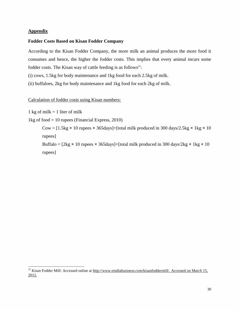
Appendix
Fodder Costs Based on Kisan Fodder Company
According to the Kisan Fodder Company, the more milk an animal produces the more food it
consumes and hence, the higher the fodder costs. This implies that every animal incurs some
fodder costs. The Kisan way of cattle feeding is as follows21:
(i) cows, 1.5kg for body maintenance and 1kg food for each 2.5kg of milk.
(ii) buffaloes, 2kg for body maintenance and 1kg food for each 2kg of milk.
Calculation of fodder costs using Kisan numbers:
1 kg of milk = 1 liter of milk
1kg of food = 10 rupees (Financial Express, 2010)
Cow = [1.5kg × 10 rupees × 365days]+[total milk produced in 300 days/2.5kg × 1kg × 10
rupees]
Buffalo = [2kg × 10 rupees × 365days]+[total milk produced in 300 days/2kg × 1kg × 10
rupees]
21
Kisan Fodder Mill: Accessed online at http://www.eindiabusiness.com/kisanfoddermill/. Accessed on March 15,
2012.