Contents lists available at ScienceDirect

Continental Shelf Research

journal homepage: www.elsevier.com/locate/csr

Simulation of river plume behaviors in a tropical region: Case study of theUpper Gulf of Thailand

Xiaojie Yua, Xinyu Guoa,⁎, Akihiko Morimotoa, Anukul Buranaprathepratb

a Center for Marine Environmental Studies (CMES), Ehime University, JapanbDepartment of Aquatic Science, Faculty of Science, Burapha University, Thailand

A R T I C L E I N F O

Keywords:River plumeLow latitudeWind effectRiver dischargeUpper Gulf of ThailandBulge size

A B S T R A C T

River plumes are a general phenomenon in coastal regions. Most previous studies focus on river plumes inmiddle and high latitudes with few studies examining those in low latitude regions. Here, we apply a numericalmodel to the Upper Gulf of Thailand (UGoT) to examine a river plume in low latitudes. Consistent with ob-servational data, the modeled plume has seasonal variation dependent on monsoon conditions. During south-westerly monsoons, the plume extends northeastward to the head of the gulf; during northeasterly monsoons, itextends southwestward to the mouth of the gulf. To examine the effects of latitude, wind and river discharge onthe river plume, we designed several numerical experiments. Using a middle latitude for the UGoT, the bulgeclose to the river mouth becomes smaller, the downstream current flows closer to the coast, and the salinity inthe northern UGoT becomes lower. The reduction in the size of the bulge is consistent with the relationshipbetween the offshore distance of a bulge and the Coriolis parameter. Momentum balance of the coastal current ismaintained by advection, the Coriolis force, pressure gradient and internal stresses in both low and middlelatitudes, with the Coriolis force and pressure gradient enlarged in the middle latitude. The larger pressuregradient in the middle latitude is induced by more offshore freshwater flowing with the coastal current, whichinduces lower salinity. The influence of wind on the river plume not only has the advection effects of changingthe surface current direction and increasing the surface current speed, but also decreases the current speed dueto enhanced vertical mixing. Changes in river discharge influence stratification in the UGoT but have little effecton the behavior of the river plume.

1. Introduction

In coastal regions, the discharge of freshwater from rivers is one ofthe principle sources of buoyancy. Through formation of a river plumewith a sharp density gradient between the buoyant freshwater and seawater, two notable characteristics emerge in the Northern hemisphere:an anticyclonic bulge in the vicinity of the river mouth and a down-stream (in a Kelvin wave sense) coastal current (Chao and Boicourt,1986). The behavior of the plume is influenced by a variety of factors,including wind (Fong, 1998; Dzwonkowski et al., 2014), the Coriolisforce (Kasai et al., 2000; Fong and Geyer, 2002), ambient currents(Fong and Geyer, 2002), tides (Guo and Valle-Levinson, 2007; Horner-Devine et al., 2009), thermal stratification (Wang et al., 2008) and riverdischarge (Yankovsky et al., 2001; Wang et al., 2011; Dzwonkowskiet al., 2014).

Most studies on river plumes are based on observations or modelanalysis conducted in middle or high latitude regions, such as theChesapeake Bay (Pritchard, 1952, 1954; Guo and Valle-Levinson,

2007), Delaware Bay (Münchow and Garvine, 1993; Wong, 1994), theColumbia River (Horner-Devine et al., 2009), and the Yellow River(Wang et al., 2008, 2011). However, fewer studies examining riverplume behaviors have been conducted in regions of low latitude. Lowlatitude regions have a small Coriolis parameter, enormous dischargesof freshwater and distinctive wind patterns (Nittrouer and DeMaster,1996). All of these factors make the behavior of river plumes in lowlatitudes significantly different from those in middle and high latitudes.

The main focus on tropical rivers has been on the Amazon River(Lentz and Limeburner, 1995; Lentz, 1995a, 1995b; Nittrouer andDeMaster, 1996), which discharges freshwater at the equator. Differingfrom river plumes in middle latitudes, which deflect to the right by theCoriolis force in the Northern Hemisphere, the Amazon River plumeextends leftward to the north Brazilian shelf between the equator and5°N under the superposition effects of the low latitude location, strongtides and easterly trade winds (Lentz, 1995a; Nittrouer and DeMaster,1996). There are also other rivers in low latitude regions, not justaround the equator, but between the equator and middle latitudes.

https://doi.org/10.1016/j.csr.2017.12.007Received 27 May 2017; Received in revised form 29 November 2017; Accepted 11 December 2017

⁎ Correspondence to: Center for Marine Environmental Studies, Ehime University, 2–5 Bunkyo-Cho, Matsuyama 790-8577, Japan.E-mail address: guoxinyu@sci.ehime-u.ac.jp (X. Guo).

Continental Shelf Research 153 (2018) 16–29

Available online 14 December 20170278-4343/ © 2017 Elsevier Ltd. All rights reserved.

T

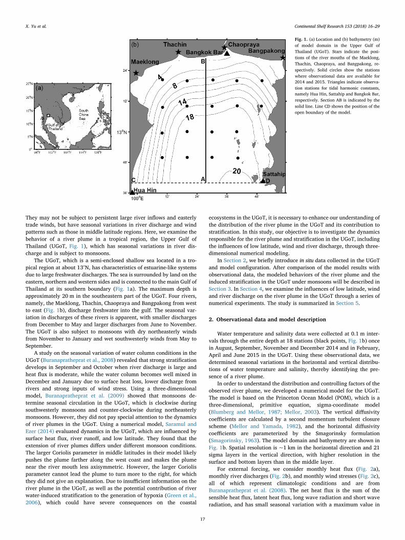
They may not be subject to persistent large river inflows and easterlytrade winds, but have seasonal variations in river discharge and windpatterns such as those in middle latitude regions. Here, we examine thebehavior of a river plume in a tropical region, the Upper Gulf ofThailand (UGoT, Fig. 1), which has seasonal variations in river dis-charge and is subject to monsoons.

The UGoT, which is a semi-enclosed shallow sea located in a tro-pical region at about 13°N, has characteristics of estuarine-like systemsdue to large freshwater discharges. The sea is surrounded by land on theeastern, northern and western sides and is connected to the main Gulf ofThailand at its southern boundary (Fig. 1a). The maximum depth isapproximately 20 m in the southeastern part of the UGoT. Four rivers,namely, the Maeklong, Thachin, Chaopraya and Bangpakong from westto east (Fig. 1b), discharge freshwater into the gulf. The seasonal var-iation in discharges of these rivers is apparent, with smaller dischargesfrom December to May and larger discharges from June to November.The UGoT is also subject to monsoons with dry northeasterly windsfrom November to January and wet southwesterly winds from May toSeptember.

A study on the seasonal variation of water column conditions in theUGoT (Buranapratheprat et al., 2008) revealed that strong stratificationdevelops in September and October when river discharge is large andheat flux is moderate, while the water column becomes well mixed inDecember and January due to surface heat loss, lower discharge fromrivers and strong inputs of wind stress. Using a three-dimensionalmodel, Buranapratheprat et al. (2009) showed that monsoons de-termine seasonal circulation in the UGoT, which is clockwise duringsouthwesterly monsoons and counter-clockwise during northeasterlymonsoons. However, they did not pay special attention to the dynamicsof river plumes in the UGoT. Using a numerical model, Saramul andEzer (2014) evaluated dynamics in the UGoT, which are influenced bysurface heat flux, river runoff, and low latitude. They found that theextension of river plumes differs under different monsoon conditions.The larger Coriolis parameter in middle latitudes in their model likelypushes the plume farther along the west coast and makes the plumenear the river mouth less axisymmetric. However, the larger Coriolisparameter cannot lead the plume to turn more to the right, for whichthey did not give an explanation. Due to insufficient information on theriver plume in the UGoT, as well as the potential contribution of riverwater-induced stratification to the generation of hypoxia (Green et al.,2006), which could have severe consequences on the coastal

ecosystems in the UGoT, it is necessary to enhance our understanding ofthe distribution of the river plume in the UGoT and its contribution tostratification. In this study, our objective is to investigate the dynamicsresponsible for the river plume and stratification in the UGoT, includingthe influences of low latitude, wind and river discharge, through three-dimensional numerical modeling.

In Section 2, we briefly introduce in situ data collected in the UGoTand model configuration. After comparison of the model results withobservational data, the modeled behaviors of the river plume and theinduced stratification in the UGoT under monsoons will be described inSection 3. In Section 4, we examine the influences of low latitude, windand river discharge on the river plume in the UGoT through a series ofnumerical experiments. The study is summarized in Section 5.

2. Observational data and model description

Water temperature and salinity data were collected at 0.1 m inter-vals through the entire depth at 18 stations (black points, Fig. 1b) oncein August, September, November and December 2014 and in February,April and June 2015 in the UGoT. Using these observational data, wedetermined seasonal variations in the horizontal and vertical distribu-tions of water temperature and salinity, thereby identifying the pre-sence of a river plume.

In order to understand the distribution and controlling factors of theobserved river plume, we developed a numerical model for the UGoT.The model is based on the Princeton Ocean Model (POM), which is athree-dimensional, primitive equation, sigma-coordinate model(Blumberg and Mellor, 1987; Mellor, 2003). The vertical diffusivitycoefficients are calculated by a second momentum turbulent closurescheme (Mellor and Yamada, 1982), and the horizontal diffusivitycoefficients are parameterized by the Smagorinsky formulation(Smagorinsky, 1963). The model domain and bathymetry are shown inFig. 1b. Spatial resolution is ~1 km in the horizontal direction and 21sigma layers in the vertical direction, with higher resolution in thesurface and bottom layers than in the middle layer.

For external forcing, we consider monthly heat flux (Fig. 2a),monthly river discharges (Fig. 2b), and monthly wind stresses (Fig. 2c),all of which represent climatologic conditions and are fromBuranapratheprat et al. (2008). The net heat flux is the sum of thesensible heat flux, latent heat flux, long wave radiation and short waveradiation, and has small seasonal variation with a maximum value in

Fig. 1. (a) Location and (b) bathymetry (m)of model domain in the Upper Gulf ofThailand (UGoT). Stars indicate the posi-tions of the river mouths of the Maeklong,Thachin, Chaopraya, and Bangpakong, re-spectively. Solid circles show the stationswhere observational data are available for2014 and 2015. Triangles indicate observa-tion stations for tidal harmonic constants,namely Hua Hin, Sattahip and Bangkok Bar,respectively. Section AB is indicated by thesolid line. Line CD shows the position of theopen boundary of the model.

X. Yu et al. Continental Shelf Research 153 (2018) 16–29

17

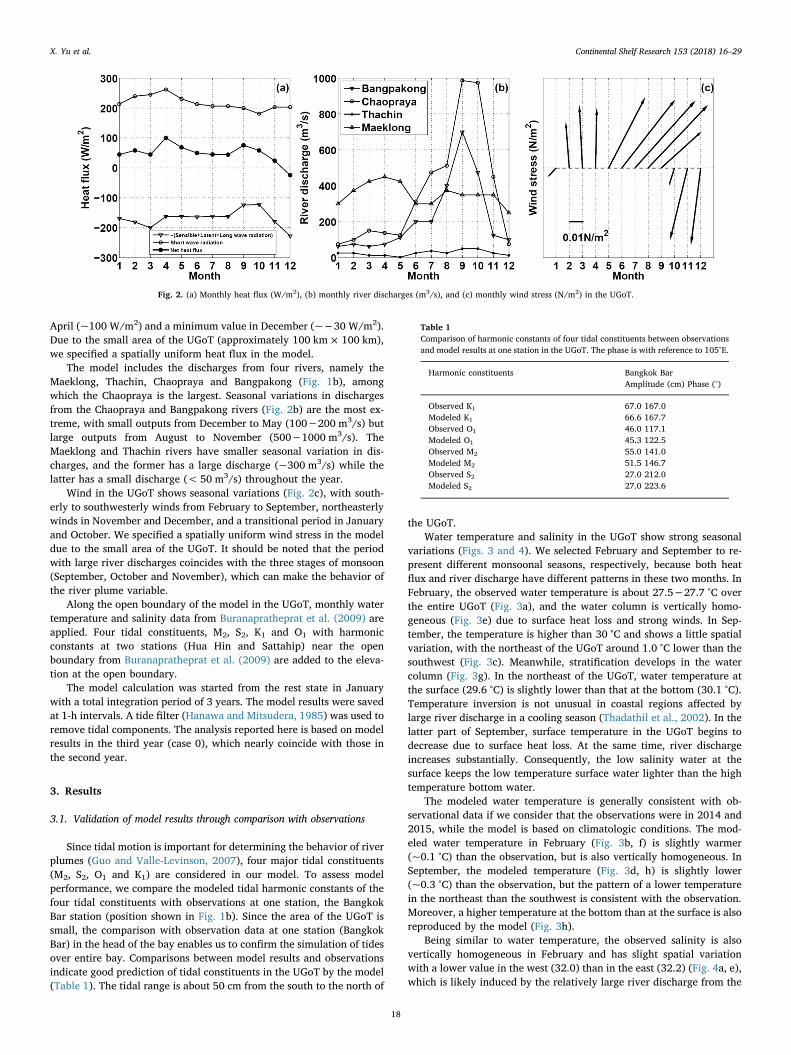
April (~100 W/m2) and a minimum value in December (~−30 W/m2).Due to the small area of the UGoT (approximately 100 km × 100 km),we specified a spatially uniform heat flux in the model.

The model includes the discharges from four rivers, namely theMaeklong, Thachin, Chaopraya and Bangpakong (Fig. 1b), amongwhich the Chaopraya is the largest. Seasonal variations in dischargesfrom the Chaopraya and Bangpakong rivers (Fig. 2b) are the most ex-treme, with small outputs from December to May (100−200 m3/s) butlarge outputs from August to November (500−1000 m3/s). TheMaeklong and Thachin rivers have smaller seasonal variation in dis-charges, and the former has a large discharge (~300 m3/s) while thelatter has a small discharge (< 50 m3/s) throughout the year.

Wind in the UGoT shows seasonal variations (Fig. 2c), with south-erly to southwesterly winds from February to September, northeasterlywinds in November and December, and a transitional period in Januaryand October. We specified a spatially uniform wind stress in the modeldue to the small area of the UGoT. It should be noted that the periodwith large river discharges coincides with the three stages of monsoon(September, October and November), which can make the behavior ofthe river plume variable.

Along the open boundary of the model in the UGoT, monthly watertemperature and salinity data from Buranapratheprat et al. (2009) areapplied. Four tidal constituents, M2, S2, K1 and O1 with harmonicconstants at two stations (Hua Hin and Sattahip) near the openboundary from Buranapratheprat et al. (2009) are added to the eleva-tion at the open boundary.

The model calculation was started from the rest state in Januarywith a total integration period of 3 years. The model results were savedat 1-h intervals. A tide filter (Hanawa and Mitsudera, 1985) was used toremove tidal components. The analysis reported here is based on modelresults in the third year (case 0), which nearly coincide with those inthe second year.

3. Results

3.1. Validation of model results through comparison with observations

Since tidal motion is important for determining the behavior of riverplumes (Guo and Valle-Levinson, 2007), four major tidal constituents(M2, S2, O1 and K1) are considered in our model. To assess modelperformance, we compare the modeled tidal harmonic constants of thefour tidal constituents with observations at one station, the BangkokBar station (position shown in Fig. 1b). Since the area of the UGoT issmall, the comparison with observation data at one station (BangkokBar) in the head of the bay enables us to confirm the simulation of tidesover entire bay. Comparisons between model results and observationsindicate good prediction of tidal constituents in the UGoT by the model(Table 1). The tidal range is about 50 cm from the south to the north of

the UGoT.Water temperature and salinity in the UGoT show strong seasonal

variations (Figs. 3 and 4). We selected February and September to re-present different monsoonal seasons, respectively, because both heatflux and river discharge have different patterns in these two months. InFebruary, the observed water temperature is about 27.5−27.7 °C overthe entire UGoT (Fig. 3a), and the water column is vertically homo-geneous (Fig. 3e) due to surface heat loss and strong winds. In Sep-tember, the temperature is higher than 30 °C and shows a little spatialvariation, with the northeast of the UGoT around 1.0 °C lower than thesouthwest (Fig. 3c). Meanwhile, stratification develops in the watercolumn (Fig. 3g). In the northeast of the UGoT, water temperature atthe surface (29.6 °C) is slightly lower than that at the bottom (30.1 °C).Temperature inversion is not unusual in coastal regions affected bylarge river discharge in a cooling season (Thadathil et al., 2002). In thelatter part of September, surface temperature in the UGoT begins todecrease due to surface heat loss. At the same time, river dischargeincreases substantially. Consequently, the low salinity water at thesurface keeps the low temperature surface water lighter than the hightemperature bottom water.

The modeled water temperature is generally consistent with ob-servational data if we consider that the observations were in 2014 and2015, while the model is based on climatologic conditions. The mod-eled water temperature in February (Fig. 3b, f) is slightly warmer(~0.1 °C) than the observation, but is also vertically homogeneous. InSeptember, the modeled temperature (Fig. 3d, h) is slightly lower(~0.3 °C) than the observation, but the pattern of a lower temperaturein the northeast than the southwest is consistent with the observation.Moreover, a higher temperature at the bottom than at the surface is alsoreproduced by the model (Fig. 3h).

Being similar to water temperature, the observed salinity is alsovertically homogeneous in February and has slight spatial variationwith a lower value in the west (32.0) than in the east (32.2) (Fig. 4a, e),which is likely induced by the relatively large river discharge from the

Fig. 2. (a) Monthly heat flux (W/m2), (b) monthly river discharges (m3/s), and (c) monthly wind stress (N/m2) in the UGoT.

Table 1Comparison of harmonic constants of four tidal constituents between observationsand model results at one station in the UGoT. The phase is with reference to 105°E.

Harmonic constituents Bangkok BarAmplitude (cm) Phase (°)

Observed K1 67.0 167.0Modeled K1 66.6 167.7Observed O1 46.0 117.1Modeled O1 45.3 122.5Observed M2 55.0 141.0Modeled M2 51.5 146.7Observed S2 27.0 212.0Modeled S2 27.0 223.6

X. Yu et al. Continental Shelf Research 153 (2018) 16–29

18

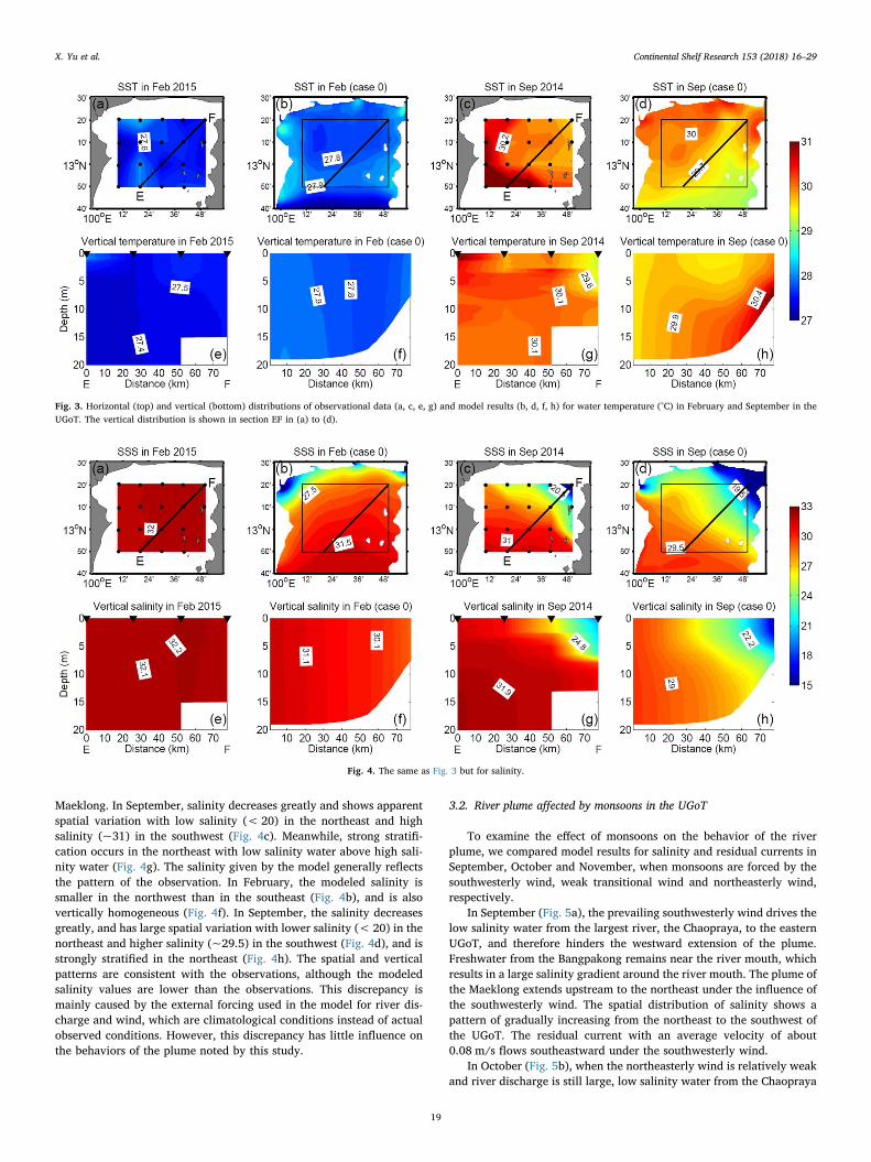
Maeklong. In September, salinity decreases greatly and shows apparentspatial variation with low salinity (< 20) in the northeast and highsalinity (~31) in the southwest (Fig. 4c). Meanwhile, strong stratifi-cation occurs in the northeast with low salinity water above high sali-nity water (Fig. 4g). The salinity given by the model generally reflectsthe pattern of the observation. In February, the modeled salinity issmaller in the northwest than in the southeast (Fig. 4b), and is alsovertically homogeneous (Fig. 4f). In September, the salinity decreasesgreatly, and has large spatial variation with lower salinity (< 20) in thenortheast and higher salinity (~29.5) in the southwest (Fig. 4d), and isstrongly stratified in the northeast (Fig. 4h). The spatial and verticalpatterns are consistent with the observations, although the modeledsalinity values are lower than the observations. This discrepancy ismainly caused by the external forcing used in the model for river dis-charge and wind, which are climatological conditions instead of actualobserved conditions. However, this discrepancy has little influence onthe behaviors of the plume noted by this study.

3.2. River plume affected by monsoons in the UGoT

To examine the effect of monsoons on the behavior of the riverplume, we compared model results for salinity and residual currents inSeptember, October and November, when monsoons are forced by thesouthwesterly wind, weak transitional wind and northeasterly wind,respectively.

In September (Fig. 5a), the prevailing southwesterly wind drives thelow salinity water from the largest river, the Chaopraya, to the easternUGoT, and therefore hinders the westward extension of the plume.Freshwater from the Bangpakong remains near the river mouth, whichresults in a large salinity gradient around the river mouth. The plume ofthe Maeklong extends upstream to the northeast under the influence ofthe southwesterly wind. The spatial distribution of salinity shows apattern of gradually increasing from the northeast to the southwest ofthe UGoT. The residual current with an average velocity of about0.08 m/s flows southeastward under the southwesterly wind.

In October (Fig. 5b), when the northeasterly wind is relatively weakand river discharge is still large, low salinity water from the Chaopraya

Fig. 3. Horizontal (top) and vertical (bottom) distributions of observational data (a, c, e, g) and model results (b, d, f, h) for water temperature (°C) in February and September in theUGoT. The vertical distribution is shown in section EF in (a) to (d).

Fig. 4. The same as Fig. 3 but for salinity.

X. Yu et al. Continental Shelf Research 153 (2018) 16–29

19

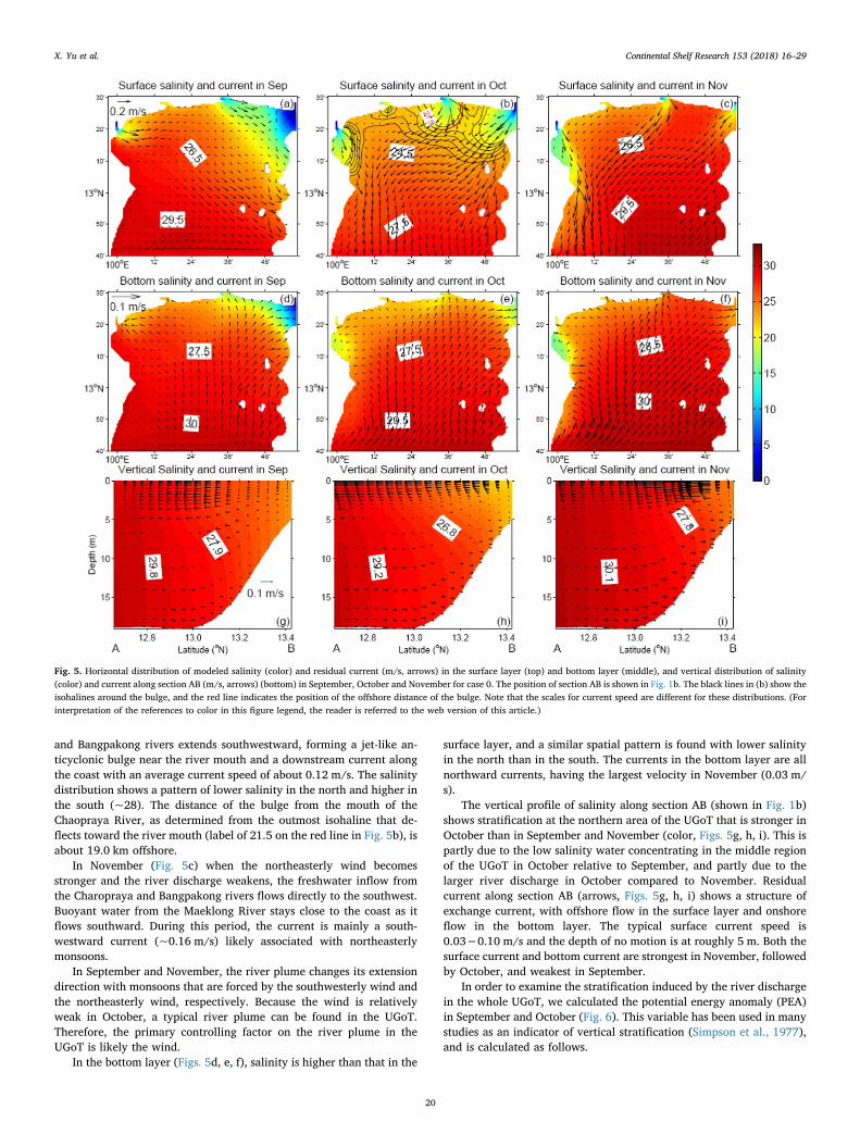
and Bangpakong rivers extends southwestward, forming a jet-like an-ticyclonic bulge near the river mouth and a downstream current alongthe coast with an average current speed of about 0.12 m/s. The salinitydistribution shows a pattern of lower salinity in the north and higher inthe south (~28). The distance of the bulge from the mouth of theChaopraya River, as determined from the outmost isohaline that de-flects toward the river mouth (label of 21.5 on the red line in Fig. 5b), isabout 19.0 km offshore.

In November (Fig. 5c) when the northeasterly wind becomesstronger and the river discharge weakens, the freshwater inflow fromthe Charopraya and Bangpakong rivers flows directly to the southwest.Buoyant water from the Maeklong River stays close to the coast as itflows southward. During this period, the current is mainly a south-westward current (~0.16 m/s) likely associated with northeasterlymonsoons.

In September and November, the river plume changes its extensiondirection with monsoons that are forced by the southwesterly wind andthe northeasterly wind, respectively. Because the wind is relativelyweak in October, a typical river plume can be found in the UGoT.Therefore, the primary controlling factor on the river plume in theUGoT is likely the wind.

In the bottom layer (Figs. 5d, e, f), salinity is higher than that in the

surface layer, and a similar spatial pattern is found with lower salinityin the north than in the south. The currents in the bottom layer are allnorthward currents, having the largest velocity in November (0.03 m/s).

The vertical profile of salinity along section AB (shown in Fig. 1b)shows stratification at the northern area of the UGoT that is stronger inOctober than in September and November (color, Figs. 5g, h, i). This ispartly due to the low salinity water concentrating in the middle regionof the UGoT in October relative to September, and partly due to thelarger river discharge in October compared to November. Residualcurrent along section AB (arrows, Figs. 5g, h, i) shows a structure ofexchange current, with offshore flow in the surface layer and onshoreflow in the bottom layer. The typical surface current speed is0.03−0.10 m/s and the depth of no motion is at roughly 5 m. Both thesurface current and bottom current are strongest in November, followedby October, and weakest in September.

In order to examine the stratification induced by the river dischargein the whole UGoT, we calculated the potential energy anomaly (PEA)in September and October (Fig. 6). This variable has been used in manystudies as an indicator of vertical stratification (Simpson et al., 1977),and is calculated as follows.

Fig. 5. Horizontal distribution of modeled salinity (color) and residual current (m/s, arrows) in the surface layer (top) and bottom layer (middle), and vertical distribution of salinity(color) and current along section AB (m/s, arrows) (bottom) in September, October and November for case 0. The position of section AB is shown in Fig. 1b. The black lines in (b) show theisohalines around the bulge, and the red line indicates the position of the offshore distance of the bulge. Note that the scales for current speed are different for these distributions. (Forinterpretation of the references to color in this figure legend, the reader is referred to the web version of this article.)

X. Yu et al. Continental Shelf Research 153 (2018) 16–29

20

∫= −−

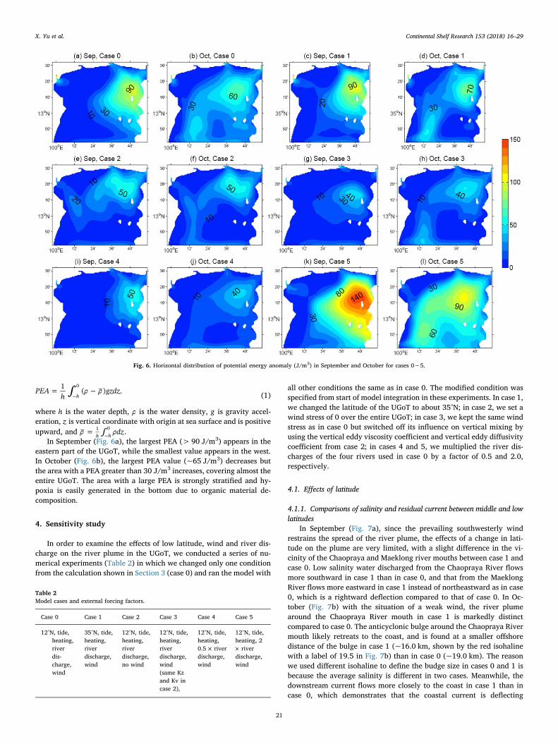
PEAh

ρ ρ gzdz1 ( ) ,h

0

(1)

where h is the water depth, ρ is the water density, g is gravity accel-eration, z is vertical coordinate with origin at sea surface and is positiveupward, and ∫=

−ρ ρdzh h

1 0 .In September (Fig. 6a), the largest PEA (> 90 J/m3) appears in the

eastern part of the UGoT, while the smallest value appears in the west.In October (Fig. 6b), the largest PEA value (~65 J/m3) decreases butthe area with a PEA greater than 30 J/m3 increases, covering almost theentire UGoT. The area with a large PEA is strongly stratified and hy-poxia is easily generated in the bottom due to organic material de-composition.

4. Sensitivity study

In order to examine the effects of low latitude, wind and river dis-charge on the river plume in the UGoT, we conducted a series of nu-merical experiments (Table 2) in which we changed only one conditionfrom the calculation shown in Section 3 (case 0) and ran the model with

all other conditions the same as in case 0. The modified condition wasspecified from start of model integration in these experiments. In case 1,we changed the latitude of the UGoT to about 35°N; in case 2, we set awind stress of 0 over the entire UGoT; in case 3, we kept the same windstress as in case 0 but switched off its influence on vertical mixing byusing the vertical eddy viscosity coefficient and vertical eddy diffusivitycoefficient from case 2; in cases 4 and 5, we multiplied the river dis-charges of the four rivers used in case 0 by a factor of 0.5 and 2.0,respectively.

4.1. Effects of latitude

4.1.1. Comparisons of salinity and residual current between middle and lowlatitudes

In September (Fig. 7a), since the prevailing southwesterly windrestrains the spread of the river plume, the effects of a change in lati-tude on the plume are very limited, with a slight difference in the vi-cinity of the Chaopraya and Maeklong river mouths between case 1 andcase 0. Low salinity water discharged from the Chaopraya River flowsmore southward in case 1 than in case 0, and that from the MaeklongRiver flows more eastward in case 1 instead of northeastward as in case0, which is a rightward deflection compared to that of case 0. In Oc-tober (Fig. 7b) with the situation of a weak wind, the river plumearound the Chaopraya River mouth in case 1 is markedly distinctcompared to case 0. The anticyclonic bulge around the Chaopraya Rivermouth likely retreats to the coast, and is found at a smaller offshoredistance of the bulge in case 1 (~16.0 km, shown by the red isohalinewith a label of 19.5 in Fig. 7b) than in case 0 (~19.0 km). The reasonwe used different isohaline to define the budge size in cases 0 and 1 isbecause the average salinity is different in two cases. Meanwhile, thedownstream current flows more closely to the coast in case 1 than incase 0, which demonstrates that the coastal current is deflecting

Fig. 6. Horizontal distribution of potential energy anomaly (J/m3) in September and October for cases 0−5.

Table 2Model cases and external forcing factors.

Case 0 Case 1 Case 2 Case 3 Case 4 Case 5

12°N, tide,heating,riverdis-charge,wind

35°N, tide,heating,riverdischarge,wind

12°N, tide,heating,riverdischarge,no wind

12°N, tide,heating,riverdischarge,wind(same Kzand Kv incase 2),

12°N, tide,heating,0.5 × riverdischarge,wind

12°N, tide,heating, 2× riverdischarge,wind

X. Yu et al. Continental Shelf Research 153 (2018) 16–29

21

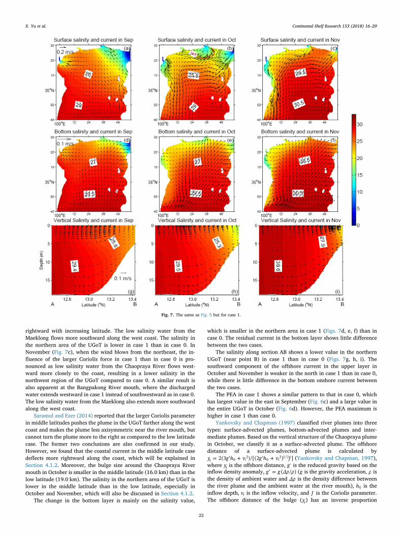
rightward with increasing latitude. The low salinity water from theMaeklong flows more southward along the west coast. The salinity inthe northern area of the UGoT is lower in case 1 than in case 0. InNovember (Fig. 7c), when the wind blows from the northeast, the in-fluence of the larger Coriolis force in case 1 than in case 0 is pro-nounced as low salinity water from the Chaopraya River flows west-ward more closely to the coast, resulting in a lower salinity in thenorthwest region of the UGoT compared to case 0. A similar result isalso apparent at the Bangpakong River mouth, where the dischargedwater extends westward in case 1 instead of southwestward as in case 0.The low salinity water from the Maeklong also extends more southwardalong the west coast.

Saramul and Ezer (2014) reported that the larger Coriolis parameterin middle latitudes pushes the plume in the UGoT farther along the westcoast and makes the plume less axisymmetric near the river mouth, butcannot turn the plume more to the right as compared to the low latitudecase. The former two conclusions are also confirmed in our study.However, we found that the coastal current in the middle latitude casedeflects more rightward along the coast, which will be explained inSection 4.1.2. Moreover, the bulge size around the Chaopraya Rivermouth in October is smaller in the middle latitude (16.0 km) than in thelow latitude (19.0 km). The salinity in the northern area of the UGoT islower in the middle latitude than in the low latitude, especially inOctober and November, which will also be discussed in Section 4.1.2.

The change in the bottom layer is mainly on the salinity value,

which is smaller in the northern area in case 1 (Figs. 7d, e, f) than incase 0. The residual current in the bottom layer shows little differencebetween the two cases.

The salinity along section AB shows a lower value in the northernUGoT (near point B) in case 1 than in case 0 (Figs. 7g, h, i). Thesouthward component of the offshore current in the upper layer inOctober and November is weaker in the north in case 1 than in case 0,while there is little difference in the bottom onshore current betweenthe two cases.

The PEA in case 1 shows a similar pattern to that in case 0, whichhas largest value in the east in September (Fig. 6c) and a large value inthe entire UGoT in October (Fig. 6d). However, the PEA maximum ishigher in case 1 than case 0.

Yankovsky and Chapman (1997) classified river plumes into threetypes: surface-advected plumes, bottom-advected plumes and inter-mediate plumes. Based on the vertical structure of the Chaopraya plumein October, we classify it as a surface-advected plume. The offshoredistance of a surface-advected plume is calculated by

= ′ + ′ +y g h v g h v f2(3 )/[(2 ) ]s i i02

02 1/2 (Yankovsky and Chapman, 1997),

where ys is the offshore distance, ′g is the reduced gravity based on theinflow density anomaly, ′ =g g Δρ ρ( / ) (g is the gravity acceleration, ρ isthe density of ambient water and Δρ is the density difference betweenthe river plume and the ambient water at the river mouth), h0 is theinflow depth, vi is the inflow velocity, and f is the Coriolis parameter.The offshore distance of the bulge (ys) has an inverse proportion

Fig. 7. The same as Fig. 5 but for case 1.

X. Yu et al. Continental Shelf Research 153 (2018) 16–29

22

relationship with the Coriolis parameter ( f ), which is 3.2 × 10−5 s−1 at13°N and 8.3 × 10−5 s−1 at 35°N. The smaller Coriolis parameter in lowlatitudes favors a larger offshore distance. This is consistent with theresult of a larger ys in the low latitude (19 km, case 0) than in themiddle latitude (16 km, case 1) in October when the wind is weak.However, the ratio of ys between the low and middle latitudes is notexactly equal to that of f1/ , indicating that the density difference be-tween the river plume and the ambient water at the river mouth ( ′g )also affects the offshore distance of the bulge because h0 and vi are thesame in different latitudes.

4.1.2. Dynamics of the bulge and coastal current in middle and low latitudesThe momentum equation for the eastward and northward velocity

of the plume can be expressed as

∂

∂+ = + +

ut

ADV COR PRE VDIFx x x x (2)

∂

∂+ = + +

vt

ADV COR PRE VDIFy y y y (3)

where ADV denotes the advection terms, COR denotes the Coriolis

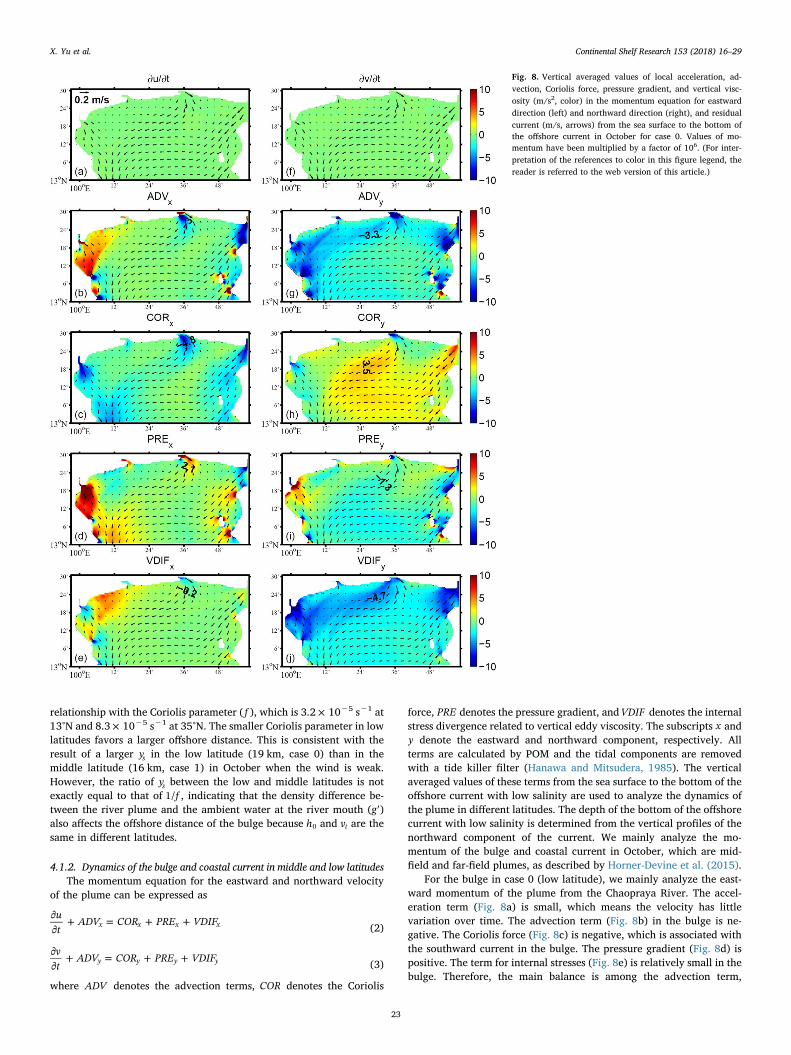
force, PRE denotes the pressure gradient, andVDIF denotes the internalstress divergence related to vertical eddy viscosity. The subscripts x andy denote the eastward and northward component, respectively. Allterms are calculated by POM and the tidal components are removedwith a tide killer filter (Hanawa and Mitsudera, 1985). The verticalaveraged values of these terms from the sea surface to the bottom of theoffshore current with low salinity are used to analyze the dynamics ofthe plume in different latitudes. The depth of the bottom of the offshorecurrent with low salinity is determined from the vertical profiles of thenorthward component of the current. We mainly analyze the mo-mentum of the bulge and coastal current in October, which are mid-field and far-field plumes, as described by Horner-Devine et al. (2015).

For the bulge in case 0 (low latitude), we mainly analyze the east-ward momentum of the plume from the Chaopraya River. The accel-eration term (Fig. 8a) is small, which means the velocity has littlevariation over time. The advection term (Fig. 8b) in the bulge is ne-gative. The Coriolis force (Fig. 8c) is negative, which is associated withthe southward current in the bulge. The pressure gradient (Fig. 8d) ispositive. The term for internal stresses (Fig. 8e) is relatively small in thebulge. Therefore, the main balance is among the advection term,

Fig. 8. Vertical averaged values of local acceleration, ad-vection, Coriolis force, pressure gradient, and vertical visc-osity (m/s2, color) in the momentum equation for eastwarddirection (left) and northward direction (right), and residualcurrent (m/s, arrows) from the sea surface to the bottom ofthe offshore current in October for case 0. Values of mo-mentum have been multiplied by a factor of 106. (For inter-pretation of the references to color in this figure legend, thereader is referred to the web version of this article.)

X. Yu et al. Continental Shelf Research 153 (2018) 16–29

23

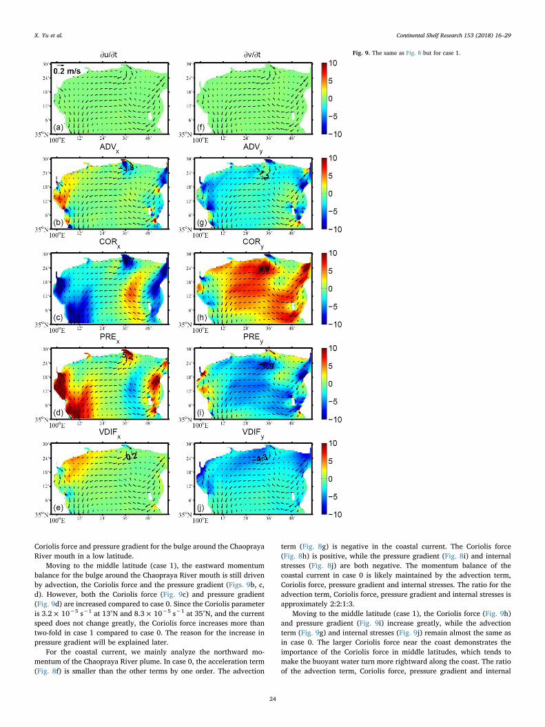
Coriolis force and pressure gradient for the bulge around the ChaoprayaRiver mouth in a low latitude.

Moving to the middle latitude (case 1), the eastward momentumbalance for the bulge around the Chaopraya River mouth is still drivenby advection, the Coriolis force and the pressure gradient (Figs. 9b, c,d). However, both the Coriolis force (Fig. 9c) and pressure gradient(Fig. 9d) are increased compared to case 0. Since the Coriolis parameteris 3.2 × 10−5 s−1 at 13°N and 8.3 × 10−5 s−1 at 35°N, and the currentspeed does not change greatly, the Coriolis force increases more thantwo-fold in case 1 compared to case 0. The reason for the increase inpressure gradient will be explained later.

For the coastal current, we mainly analyze the northward mo-mentum of the Chaopraya River plume. In case 0, the acceleration term(Fig. 8f) is smaller than the other terms by one order. The advection

term (Fig. 8g) is negative in the coastal current. The Coriolis force(Fig. 8h) is positive, while the pressure gradient (Fig. 8i) and internalstresses (Fig. 8j) are both negative. The momentum balance of thecoastal current in case 0 is likely maintained by the advection term,Coriolis force, pressure gradient and internal stresses. The ratio for theadvection term, Coriolis force, pressure gradient and internal stresses isapproximately 2:2:1:3.

Moving to the middle latitude (case 1), the Coriolis force (Fig. 9h)and pressure gradient (Fig. 9i) increase greatly, while the advectionterm (Fig. 9g) and internal stresses (Fig. 9j) remain almost the same asin case 0. The larger Coriolis force near the coast demonstrates theimportance of the Coriolis force in middle latitudes, which tends tomake the buoyant water turn more rightward along the coast. The ratioof the advection term, Coriolis force, pressure gradient and internal

Fig. 9. The same as Fig. 8 but for case 1.

X. Yu et al. Continental Shelf Research 153 (2018) 16–29

24

stresses is approximately 1:6:4:3 in the middle latitude, indicating thatthe coastal current in the middle latitude becomes more geostrophicrelative to that in the low latitude.

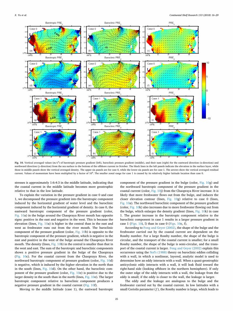
To explain the variation in the pressure gradient in case 0 and case1, we decomposed the pressure gradient into the barotropic componentinduced by the horizontal gradient of water level and the barocliniccomponent induced by the horizontal gradient of density. In case 0, theeastward barotropic component of the pressure gradient (color,Fig. 10a) in the bulge around the Chaopraya River mouth has oppositesigns: positive in the east and negative in the west. This is because theelevation (lines, Fig. 10a) is higher in the central than in the east andwest as freshwater runs out from the river mouth. The barocliniccomponent of the pressure gradient (color, Fig. 10b) is opposite to thebarotropic component of the pressure gradient, which is negative in theeast and positive in the west of the bulge around the Chaopraya Rivermouth. The density (lines, Fig. 10b) in the central is smaller than that inthe west and east. The sum of the barotropic and baroclinic componentsshows a positive pressure gradient in the bulge of the Chaopraya(Fig. 10c). For the coastal current from the Chaopraya River, thenorthward barotropic component of pressure gradient (color, Fig. 10d)is negative, which is induced by the higher elevation in the north thanin the south (lines, Fig. 10d). On the other hand, the baroclinic com-ponent of the pressure gradient (color, Fig. 10e) is positive due to thelarger density in the south than in the north (lines, Fig. 10e). The largerbarotropic component relative to baroclinic component produces anegative pressure gradient in the coastal current (Fig. 10f).

Moving to the middle latitude (case 1), the eastward barotropic

component of the pressure gradient in the bulge (color, Fig. 10g) andthe northward barotropic component of the pressure gradient in thecoastal current (color, Fig. 10j) from the Chaopraya River increase. It islikely that more freshwater flows out from the bulge, and induces thecloser elevation contour (lines, Fig. 10g) relative to case 0 (lines,Fig. 10a). The northward baroclinic component of the pressure gradient(color, Fig. 10k) also increases due to more freshwater flowing out fromthe bulge, which enlarges the density gradient (lines, Fig. 10k) in case1. The greater increase in the barotropic component relative to thebaroclinic component in case 1 results in a larger pressure gradient incase 1 (Figs. 10i, l) than in case 0 (Figs. 10c, f).

According to Fong and Geyer (2002), the shape of the bulge and thefreshwater carried out by the coastal current are dependent on theRossby number. For a large Rossby number, the shape of the bulge iscircular, and the transport of the coastal current is smaller; for a smallRossby number, the shape of the bulge is semi-circular, and the trans-port of the coastal current is larger. Fong and Geyer (2002) explain thisoccurrence using the Nof's (1988) theory on baroclinic eddies collidingwith a wall, in which a nonlinear, layered, analytic model is used todetermine how an eddy interacts with a wall. When a quasi-geostrophicanticyclonic eddy interacts with a wall, it will leak fluid toward theright-hand side (looking offshore in the northern hemisphere). If onlythe outer edge of the eddy interacts with a wall, the leakage from theeddy is small; if the eddy is closer to the wall, the leakage is larger.

The eddy and the leakage are analogous to the bulge and thefreshwater carried out by the coastal current. In low latitudes with asmall Coriolis parameter ( f ), the Rossby number is large, which leads to

Fig. 10. Vertical averaged values (m/s2) of barotropic pressure gradient (left), baroclinic pressure gradient (middle), and their sum (right) for the eastward direction (x-direction) andnorthward direction (y-direction) from the sea surface to the bottom of the offshore current in October. The black lines in the left panels indicate the elevation in the surface layer, whilethose in middle panels show the vertical averaged density. The upper six panels are for case 0, while the lower six panels are for case 1. The arrows show the vertical averaged residualcurrent. Values of momentum have been multiplied by a factor of 106. The smaller zonal range for case 1 is caused by its relatively higher latitude location than case 0.

X. Yu et al. Continental Shelf Research 153 (2018) 16–29

25

a large offshore distance of the bulge (eddy away from the wall), andconsequently the freshwater quantity flowing with the coastal current issmaller. In middle latitudes, the situation is opposite; that is, the bulgeis smaller (eddy close to the wall) and the freshwater quantity flowingwith the coastal current is larger. This can explain why the barotropicand baroclinic pressure gradient is larger in the middle latitude than in

the low latitude, as well as the lower salinity in the northern UGoT incase 1 than in case 0.

4.2. Effects of wind

The effect of wind on the coastal region is manifested not only in the

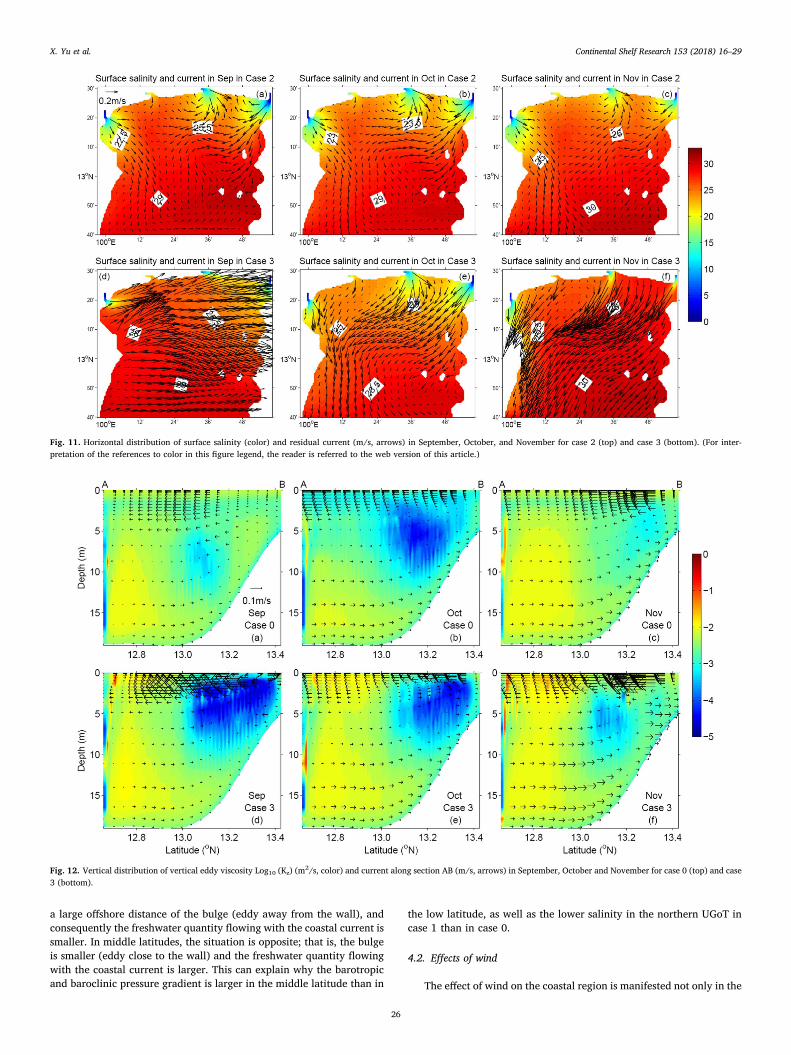
Fig. 11. Horizontal distribution of surface salinity (color) and residual current (m/s, arrows) in September, October, and November for case 2 (top) and case 3 (bottom). (For inter-pretation of the references to color in this figure legend, the reader is referred to the web version of this article.)

Fig. 12. Vertical distribution of vertical eddy viscosity Log10 (Kz) (m2/s, color) and current along section AB (m/s, arrows) in September, October and November for case 0 (top) and case3 (bottom).

X. Yu et al. Continental Shelf Research 153 (2018) 16–29

26

changing surface current but also in producing enhanced verticalmixing in the upper layer. To separately examine the two effects ofwind on the river plume, we consider the situation of no wind in case 2and the situation of wind but without wind-enhanced vertical mixing incase 3 by using the vertical eddy viscosity and diffusivity from case 2.

In case 2, when there is no wind, the structures of the river plume in

different months are almost identical, with a bulge forming near theriver mouth, and a downstream current flowing along the coast(Figs. 11a, b, c). The only difference among the months is the salinityvalue and current speed, which are determined by monthly river dis-charges. The coastal current speed from the Chaopraya River is 0.18,0.15, and 0.11 m/s in September, October, and November, respectively.

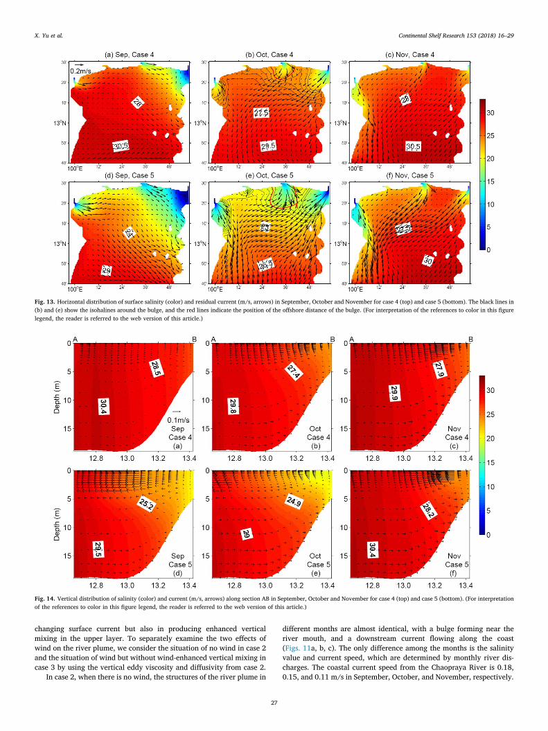
Fig. 13. Horizontal distribution of surface salinity (color) and residual current (m/s, arrows) in September, October and November for case 4 (top) and case 5 (bottom). The black lines in(b) and (e) show the isohalines around the bulge, and the red lines indicate the position of the offshore distance of the bulge. (For interpretation of the references to color in this figurelegend, the reader is referred to the web version of this article.)

Fig. 14. Vertical distribution of salinity (color) and current (m/s, arrows) along section AB in September, October and November for case 4 (top) and case 5 (bottom). (For interpretationof the references to color in this figure legend, the reader is referred to the web version of this article.)

X. Yu et al. Continental Shelf Research 153 (2018) 16–29

27

The PEA shows a similar pattern in September and October (Figs. 6e, f),with a large value around the Chaopraya and Bangpakong rivers, and ahigher value in September due to larger river discharge.

In case 3, the surface currents (Figs. 11d, e, f) are different fromthose in case 2, but show a resemblance to those in case 0 in currentdirection with a larger current speed than case 0. Comparison of case 3and case 2 shows a wind-induced surface current in case 3 that flowsnortheastward in September and southwestward in October and No-vember under the southwesterly and northeasterly winds, respectively.The coastal current speed from the Chaopraya River in case 3 is 0.36,0.22, and 0.40 m/s in September, October, and November, respectively.Comparison of case 3 with case 0 shows the effect of wind instrengthening the vertical mixing, which weakens the current speed incase 0，especially in the northern area of 13°N. The distribution of PEAin case 3 shows a similar pattern to that in case 0, which is large in theeast in September and large in the entire UGoT in October (Figs. 6g, h).

Wind produces large vertical eddy viscosity in case 0 (color,Figs. 12a, b, c) relative to cases 2 and 3 (color, Figs. 12d, e, f) in theupper layer north of 13°N. Large eddy viscosity results in strong internalfriction and therefore weakens the current speed in the surface layer incase 0 (arrows, Fig. 12). Weaker offshore current in the surface layerinduces a weaker onshore current in the bottom layer in case 0 (arrows,Fig. 12).

4.3. Effects of river discharge

We examined the influence of river discharge on the river plume bycutting it in half and doubling in cases 4 and 5, respectively. In case 4(case 5), expansions of the river plume (Fig. 13) are similar to those incase 0, but with higher (lower) salinity and weaker (stronger) down-stream current than in case 0. The offshore distance of the bulge fromthe Chaopraya River in October increases from 15.7 km in case 4 to23.5 km in case 5 (red lines, Figs. 13b, e). The coastal current from theChaopraya River in October also turns more rightward (looking off-shore) with increasing river discharge. The response of the plume to themagnitude of the river discharge in the UGoT is similar to that in theYellow River (Wang et al., 2008) in both plume range and orientation.

The vertical profiles of salinity show the strongest stratification incase 5 (color, Figs. 14d, e, f), followed by case 0 (color, Figs. 5g, h, i)and case 4 (color, Figs. 14a, b, c) in the northern part of the UGoT. Thelarger river discharge and stronger stratification enhance the surfaceoffshore current and bottom onshore current in case 5 (arrows,Figs. 14d, e, f).

The patterns of PEA in cases 4 and 5 are similar to those in case 0,but with a smaller maximum value in case 4 (Figs. 6i, j) and a larger onein case 5 (Figs. 6k, l). The largest PEA in case 4 is 50 J/m3 in Septemberand 40 J/m3 in October, while it is 140 J/m3 and 95 J/m3 in case 5.Therefore, the river discharge can significantly change stratification inthe UGoT in the rainy season, and influence the situation of hypoxiathere.

5. Conclusion

Differing from the Amazon River plume that extends leftward to thenorthern hemisphere, in the UGoT, the river plume from four rivers inthe head of the gulf is significantly influenced by monsoons. The riverplume extends northeastward under southwesterly winds during theperiod from May to September and southwestward under northeasterlywinds during the period from November to January. In October, atransitional period for monsoons with lower wind speeds, a typical riverplume with an anticyclonic bulge near the river mouth and a down-stream current along the coast can be found in the UGoT. Stratificationinduced by river discharge is also influenced by monsoons, and is strongin the eastern part of the gulf in September but expands over the entiregulf in October, which has importance on the generation of hypoxia inthe UGoT.

Changing the model domain to the middle latitude results in a dif-ferent river plume in the UGoT. The bulge near the river mouth extendsfarther offshore in the low latitude than in the middle latitude, whichcan be qualitatively explained by the inverse relationship between theoffshore distance of bulge and the Coriolis parameter in a surface-ad-vected plume (Yankovsky and Chapman, 1997). Geostrophic control onthe coastal current of the plume is weaker in the low latitude than in themiddle latitude, which induces a smaller rightward deflected angle ofthe coastal current in the low latitude than in the middle latitude.Furthermore, salinity in the model domain is higher in the low latitudethan in the middle latitude. This is associated with less freshwater beingcarried out by the coastal current from the bulge in the low latitudethan in the middle latitude, which is consistent with the theory of Nof(1988). All these points were either not reported by or are differentfrom the previous study on the river plume in the UGoT (Saramul andEzer, 2014).

Wind has two effects on the surface current that acts as the ambientcurrent of the river plume: directly changing the surface current withthe addition of momentum to the water and indirectly changing thesurface current with enhancement of vertical mixing. These effects havenot been reported in previous studies. River discharge can change thesize of the bulge and the strength of the coastal current of the riverplume. It also significantly influences stratification in the UGoT. Alarger river discharge tends to induce stronger stratification.

Acknowledgements

This study was supported by JSPS KAKENHI Grant Number26302001 and by grants from the government to national universitycorporations for the Joint Usage/Research Center, MEXT, Japan andJSPS Core-to-Core Program.

References

Blumberg, A.F., Mellor, G.L., 1987. A description of a three dimensional coastal oceancirculation model. In: Heaps, N. (Ed.), Three-Dimensional Coastal Ocean Models,Coastal Estuarine Stud. 4. AGU, Washington, D.C., pp. 1–16 (208pp).

Buranapratheprat, A., Yanagi, T., Matsumura, S., 2008. Seasonal variation in watercolumn conditions in the upper Gulf of Thailand. Cont. Shelf Res. 28, 2509–2522.

Buranapratheprat, A., Niemann, K.O., Yanagi, T., Matsumura, S., Sojisuporn, P., 2009.Circulation in the upper Gulf of Thailand investigated using a three-dimensionalhydrodynamic model. Burapha Sci. J. 14 (1), 99–113.

Chao, S.-Y., Boicourt, W.C., 1986. Onset of estuarine plumes. J. Phys. Oceanogr. 16,2137–2149.

Dzwonkowski, B., Park, K., Lee, J., Webb, B.M., Valle-Levinson, A., 2014. Spatial varia-bility of flow over a river-influenced inner shelf in coastal Alabama during spring.Cont. Shelf Res. 74, 25–34.

Fong, D.A., 1998. Dynamics of Freshwater Plumes: Observations and NumericalModelling of the Wind-forced Response and Alongshore Freshwater Transport (Ph.D.Dissertation). MIT-Woods Hole Oceanographic Institution.

Fong, D.A., Geyer, W.R., 2002. The alongshore transport of freshwater in a surface-trapped river plume. J. Phys. Oceanogr. 32, 957–972.

Green, R.E., Bianchi, T.S., Dagg, M.J., Walker, N.D., Breed, G.A., 2006. An organic carbonbudget for the Mississippi River turbidity plume and plume contributions to air–seaCO2 fluxes and bottom water hypoxia. Estuaries Coasts 29, 579–597.

Guo, X., Valle-Levinson, A., 2007. Tidal effects on estuarine circulation and outflowplume in the Chesapeake Bay. Cont. Shelf Res. 27, 20–42.

Hanawa, K., Mitsudera, H., 1985. On daily average of oceanographic data (in Japanese).Coast. Oceanogr. Bullet 23, 79–87.

Horner-Devine, A., Jay, D., Orton, P., Spahn, E., 2009. A conceptual model of the stronglytidal Columbia River plume. J. Mar. Syst. 78, 460–475.

Horner-Devine, A., Hetland, R., MacDonald, D., 2015. Mixing and transport in coastalriver plumes. Annu. Rev. Fluid Mech. 47, 569–594.

Kasai, A., Hill, A.E., Fujiwara, T., Simpson, J.H., 2000. Effect of the Earth's rotation on thecirculation in regions of freshwater influence. J. Geophys. Res. 105 (C7),16961–16969.

Lentz, S.J., 1995a. Seasonal variations in the horizontal structure of the Amazon Plumeinferred from historical hydrographic data. J. Geophys. Res. 100, 2391–2400.

Lentz, S.J., 1995b. The Amazon River Plume during AMASSEDS: subtidal current varia-bility and the importance of wind forcing. J. Geophys. Res. 100, 2377–2390.

Lentz, S.J., Limeburner, R., 1995. The Amazon River plume during AMASSEDS: spatialcharacteristics and salinity variability. J. Geophys. Res. 100 (C2), 2355–2375.

Mellor, G.L., 2003. Users guide for a three-dimensional, primitive equation, numericalocean model (2003 version) (report, 53 pp.). Program in Atmosphere and OceanScience. Princeton Univ., Princeton, N. J.

X. Yu et al. Continental Shelf Research 153 (2018) 16–29

28

Mellor, G.L., Yamada, T., 1982. Development of a turbulence closure model for geo-physical fluid problems. Rev. Geophys. 20, 851–875.

Münchow, A., Garvine, R.W., 1993. Dynamical properties of a buoyancy-driven coastalcurrent. J. Geophys. Res. 98 (C11), 20063–20077.

Nittrouer, C.A., DeMaster, D.J., 1996. The Amazon shelf setting: tropical, energetic, andinfluenced by a large river. Cont. Shelf Res. 16, 553–573.

Nof, D., 1988. Eddy-wall interactions. J. Mar. Res. 46, 527–555.Pritchard, D.W., 1952. Salinity distribution and circulation in the Chesapeake Bay es-

tuarine system. J. Mar. Res. 11, 106–123.Pritchard, D.W., 1954. A study on the salt balance in a coastal plain estuary. J. Mar. Res.

13, 133–144.Saramul, S., Ezer, T., 2014. On the dynamics of low latitude, wide and shallow coastal

system: numerical simulations of the Upper Gulf of Thailand. Ocean Dyn. 64,557–571.

Simpson, J.H., Hughes, D.G., Morris, N.C.G., 1977. The relation of seasonal stratificationto tidal mixing on the continental shelf. Deep Sea Res. 24 (Suppl), 327–340.

Smagorinsky, J.S., 1963. General circulation experiments with the primitive equations. I.The basic experiment. Mon. Weather Rev. 91, 99–164.

Thadathil, P., Gopalakrishna, V.V., Muraleedharan, P.M., Reddy, G.V., Araligidad, N.,Shenoy, S., 2002. Surface layer temperature inversion in the Bay of Bengal. Deep SeaRes. Part Ⅰ 49, 1801–1818.

Wang, Q., Guo, X., Takeoka, H., 2008. Seasonal variations of the Yellow River plume inthe Bohai Sea: a model study. J. Geophys. Res. 113, C08046.

Wang, Y., Liu, Z., Gao, H., Ju, L., Guo, X., 2011. Response of salinity distribution aroundthe Yellow River mouth to abrupt changes in river discharge. Cont. Shelf Res. 31,685–694.

Wong, K.-C., 1994. On the nature of transverse variability in a coastal plain estuary. J.Geophys. Res. 99, 14209–14222.

Yankovsky, A.E., Chapman, D.C., 1997. A simple theory for the fate of buoyant coastaldischarges. J. Phys. Oceanogr. 27, 1386–1401.

Yankovsky, A.E., Hickey, B.M., Münchow, A.K., 2001. Impact of variable inflow on thedynamics of a coastal plume. J. Geophys. Res. 106, 19809–19824.

X. Yu et al. Continental Shelf Research 153 (2018) 16–29

29