3 Continental drift

CONTINENTAL DRIFT 55

3.1 INTRODUCTION

As early as the 16th century it had been noted that the western and eastern coastlines of the Atlantic Ocean appeared to fi t together like the pieces of a jigsaw puzzle (Section 1.1). The signifi cance of this observation was not fully realized, however, until the 19th century, when the geometric fi t of continental outlines was invoked as a major item of evidence in constructing the hypothesis of continental drift. The case for the hypothesis was further strengthened by the correspondence of geologic features across the juxtaposed coastlines. Application of the technique of paleomagnetism in the 1950s and 1960s provided the fi rst quantitative evidence that continents had moved at least in a north–south direction during geologic time. Moreover, it was demonstrated that the continents had undergone relative motions, and this confi rmed that continental drift had actually occurred.

3.2 CONTINENTAL RECONSTRUCTIONS

3.2.1 Euler’s theorem

In order to perform accurate continental reconstructions across closed oceans it is necessary to be able to describe mathematically the operation involved in making the geometric fi t. This is accomplished according to a theorem of Euler, which states that the movement of a portion of a sphere across its surface is uniquely defi ned by a single angular rotation about a pole of rotation (Fig. 3.1). The pole of rotation, and its antipodal point on the opposite diameter of the sphere, are the only two points which remain in a fi xed position relative to the moving portion. Consequently, the movement of a continent across the surface of the Earth to its pre-drift position can be described by its pole and angle of rotation.

3.2.2 Geometric reconstructions of continents

Although approximate reconstructions can be per-formed manually by moving models of continents

across an accurately constructed globe (Carey, 1958), the most rigorous reconstructions are performed mathe-matically by computer, as in this way it is possible to minimize the degree of misfi t between the juxtaposed continental margins.

The technique generally adopted in computer-based continental fi tting is to assume a series of poles of rotation for each pair of continents arranged in a grid of latitude and longitude positions. For each pole position the angle of rotation is determined that brings the continental margins together with the smallest proportion of gaps and overlaps. The fi t is not made on the coastlines, as continental crust extends beneath the surrounding shelf seas out to the continental slope. Consequently, the true junction between continental and oceanic lithosphere is taken to be at some isobath marking the midpoint of the continental slope, for example the 1000 m contour. Having determined the angle of rotation, the good-ness of fi t is quantifi ed by some criterion based on the degree of mismatch. This goodness of fi t is generally known as the objective function. Values of the objec-tive function are entered on the grid of pole positions and contoured. The location of the minimum objec-tive function revealed by this procedure then provides the pole of rotation for which the continental edges fi t most exactly.

Geographical pole

Axis of rotationPole of rotationAngle of rotation

Great circle orEquator of rotation

Small circles orlatitudes of rotation

Figure 3.1 Euler’s theorem. Diagram illustrating how the motion of a continent on the Earth can be described by an angle of rotation about a pole of rotation.

56 CHAPTER 3

3.2.3 The reconstruction of continents around the Atlantic

The fi rst mathematical reassembly of continents based solely on geometric criteria was performed by Bullard et al. (1965), who fi tted together the continents on either

side of the Atlantic (Fig. 3.2). This was accomplished by sequentially fi tting pairs of continents after determining their best fi tting poles of rotation by the procedure described in Section 3.2.2. The only rotation involving parts of the same landmass is that of the Iberian penin-sular with respect to the rest of Europe. This is justifi ed because of the known presence of oceanic lithosphere

Figure 3.2 Fit of the continents around the Atlantic Ocean, obtained by matching the 500 fathom (920 m) isobath (redrawn from Bullard et al., 1965, with permission from the Royal Society of London).

CONTINENTAL DRIFT 57

in the Bay of Biscay which is closed by this rotation. Geologic evidence (Section 3.3) and information pro-vided by magnetic lineations in the Atlantic (Section 4.1.7) indicate that the reconstruction represents the continental confi guration during late Triassic/early Jurassic times approximately 200 Ma ago.

Examination of Fig. 3.2 reveals a number of overlaps of geologic signifi cance, some of which may be related to the process of stretching and thinning during the formation of rifted continental margins (Section 7.7). Iceland is absent because it is of Cenozoic age and its construction during the opening of the Atlantic post-dates the reconstruction. The Bahama Platform appears to overlap the African continental margin and main-land. It is probable, however, that the platform repre-sents an accumulation of sediment capped by coral on oceanic crust that formed after the Americas separated (Dietz & Holden, 1970). Similarly, the Niger Delta of Africa appears to form an overlap when in fact it also developed in part on oceanic crust formed after rifting.

A major criticism of the reconstruction is the overlap of Central America on to South America and absence of the Caribbean Sea. This must be viewed, however, in the light of our knowledge of the history of the opening of the Atlantic based, for the most part, on its

pattern of magnetic lineations. Geologic and geometric considerations suggest that the Paleozoic crustal blocks which underlie Central America were originally situ-ated within the region now occupied by the Gulf of México, an area existing within the reconstruction (Fig. 3.3). The North Atlantic started to open about 180 Ma ago, and the South Atlantic somewhat later, about 130 Ma ago. The poles of rotation of the North and South Atlantic were suffi ciently different that the opening created the space between North and South America now occupied by the Caribbean. This also allowed a clockwise rotation of the Central American blocks out of the Gulf of México to their present loca-tions. About 80 Ma ago the poles of rotation of the North and South Atlantic changed to an almost identi-cal location in the region of the present north pole so that from this time the whole Atlantic Ocean effectively opened as a single unit.

3.2.4 The reconstruction of Gondwana

Geometric evidence alone has also been used in the reconstruction of the southern continents that make up

Yucatan block

Chortis block

110˚ 100˚ 90˚ 80˚

30˚

20˚

30˚

C

20˚

100˚ 90˚ 80˚0 400 km

Figure 3.3 Reconstruction of the Central American region within the Bullard et al. fi t of the continents around the Atlantic (Fig. 3.2). C, location of pre-Mesozoic portions of Cuba (redrawn from White, 1980, with permission from Nature 283, 823–6. Copyright 1980 Macmillan Publishers Ltd).

58 CHAPTER 3

Gondwana. The fi rst such reconstruction was per-formed by Smith & Hallam (1970) and is illustrated in Fig. 3.4. The shapes of the continental edges of the east coast of Africa, Madagascar, India, Australia, and Ant-arctica are not quite so well suited to fi tting as the circum-Atlantic continents. However this reconstruc-tion has been confi rmed by subsequent analysis of the record of magnetic lineations in the Indian Ocean (Section 4.1.7).

3.3 GEOLOGIC EVIDENCE FOR CONTINENTAL DRIFT

The continental reconstructions discussed in Sections 3.2.3 and 3.2.4 are based solely on the geometric fi t of continental shelf edges. If they represent the true ancient confi gurations of continents it should be pos-sible to trace continuous geologic features from one continent to another across the fi ts. The matching of features requires the rifting of the supercontinent across the general trend of geologic features. This does

not always occur as the location of the rift is often controlled by the geology of the supercontinent, and takes place along lines of weakness that may run paral-lel to the geologic grain. However, there remain many geologic features that can be correlated across juxta-posed continental margins, some of which are listed below.

1 Fold belts. The continuity of the Appalachian fold belt of eastern North America with the Caledonian fold belt of northern Europe, illustrated in Fig. 3.5, is a particularly well-studied example (Dewey, 1969). Within the sedimentary deposits associated with fold belts there is often further evidence for continental drift. The grain size, composition, and age distribution of detrital zircon minerals in the sediments can be used to determine the nature and direction of their source. The source of sediments in the Caledonides of northern Europe lies to the west in a location now occupied by the Atlantic, indicating that, in the past, this location must have been occupied by continental crust (Rainbird et al., 2001; Cawood et al., 2003).

2 Age provinces. The correlation of the patterns of ages across the southern Atlantic is shown in Fig. 3.6, which illustrates the matching of both

Figure 3.4 Fit of the southern continents and India (redrawn from Smith & Hallam, 1970, with permission from Nature 225, 139–44. Copyright 1970 Macmillan Publishers Ltd).

CONTINENTAL DRIFT 59

Precambrian cratons and rocks of Paleozoic age (Hallam, 1975).

3 Igneous provinces. Distinctive igneous rocks can be traced between continents as shown in Fig. 3.7. This applies both to extrusive and intrusive rocks, such as the belt of Mesozoic dolerite, which extends through southern Africa, Antarctica, and Tasmania, and the approxi-mately linear trend of Precambrian anorthosites (Section 11.4.1) through Africa, Madagascar, and India (Smith & Hallam, 1970).

4 Stratigraphic sections. Distinctive stratigraphic sequences can also be correlated between adjacent continents. Figure 3.8 shows stratigraphic sections of the Gondwana succession, a terrestrial sequence of sediments of late Paleozoic age (Hurley, 1968). Marker beds of tillite and coal, and sediments containing Glossopteris and Gangamopteris fl ora (Section 3.5) can be correlated through South America, South Africa, Antarctica, India, and Australia.

Baltic shield

Russianplatform

African ForelandG

reen

land

Figure 3.5 The fi t of the continents around the North Atlantic, after Bullard et al. (1965), and the trends of the Appalachian-Caledonian and Variscan (early and late Paleozoic) fold belts (dark and light shading respectively). The two phases of mountain building are superimposed in eastern North America (redraw from Hurley, 1968; the Confi rmation of Continental Drift. Copyright © 1968 by Scientifi c American, Inc. All rights reserved.)

Figure 3.6 Correlation of cratons and younger mobile belts across the closed southern Atlantic Ocean (redrawn from Hurley, 1968, the Confi rmation of Continental Drift. Copyright © 1968 by Scientifi c American, Inc. All rights reserved.)

60 CHAPTER 3

5 Metallogenic provinces. Regions containing manganese, iron ore, gold, and tin can be matched across adjacent coastlines on such reconstructions (Evans, 1987).

3.4 PALEOCLIMATOLOGY

The distribution of climatic regions on the Earth is controlled by a complex interaction of many phenom-ena, including solar fl ux (i.e. latitude), wind directions, ocean currents, elevation, and topographic barriers (Sections 13.1.2, 13.1.3). The majority of these phe-nomena are only poorly known in the geologic record. On a broad scale, however, latitude is the major con-trolling factor of climate and, ignoring small micro-climatic regions dependent on rare combinations of other phenomena, it appears likely that the study of climatic indicators in ancient rocks can be used to infer, in a general sense, their ancient latitude. Consequently,

Figure 3.7 Correlation of Permo-Carboniferous glacial deposits, Mesozoic dolerites, and Precambrian anorthosites between the reconstructed continents of Gondwana (after Smith & Hallam, 1970, with permission from Nature 225, 139–44. Copyright 1970 Macmillan Publishers Ltd).

Figure 3.8 Correlation of stratigraphy between Gondwana continents (redrawn from Hurley, 1968, the Confi rmation of Continental Drift. Copyright © 1968 by Scientifi c American, Inc. All rights reserved.)

CONTINENTAL DRIFT 61

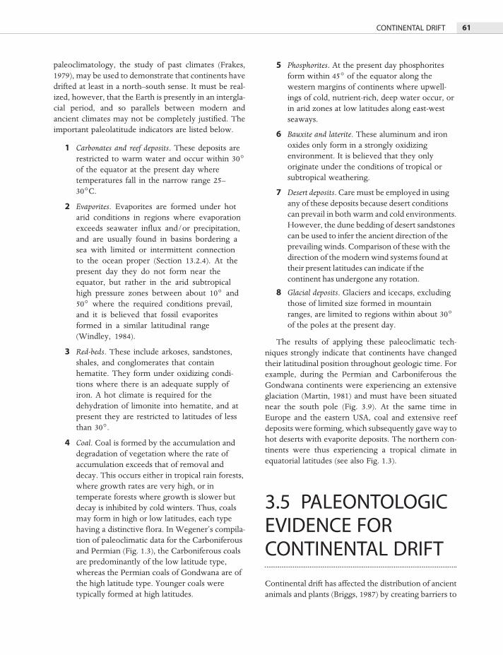
paleoclimatology, the study of past climates (Frakes, 1979), may be used to demonstrate that continents have drifted at least in a north–south sense. It must be real-ized, however, that the Earth is presently in an intergla-cial period, and so parallels between modern and ancient climates may not be completely justifi ed. The important paleolatitude indicators are listed below.

1 Carbonates and reef deposits. These deposits are restricted to warm water and occur within 30° of the equator at the present day where temperatures fall in the narrow range 25–30°C.

2 Evaporites. Evaporites are formed under hot arid conditions in regions where evaporation exceeds seawater infl ux and/or precipitation, and are usually found in basins bordering a sea with limited or intermittent connection to the ocean proper (Section 13.2.4). At the present day they do not form near the equator, but rather in the arid subtropical high pressure zones between about 10° and 50° where the required conditions prevail, and it is believed that fossil evaporites formed in a similar latitudinal range (Windley, 1984).

3 Red-beds. These include arkoses, sandstones, shales, and conglomerates that contain hematite. They form under oxidizing condi-tions where there is an adequate supply of iron. A hot climate is required for the dehydration of limonite into hematite, and at present they are restricted to latitudes of less than 30°.

4 Coal. Coal is formed by the accumulation and degradation of vegetation where the rate of accumulation exceeds that of removal and decay. This occurs either in tropical rain forests, where growth rates are very high, or in temperate forests where growth is slower but decay is inhibited by cold winters. Thus, coals may form in high or low latitudes, each type having a distinctive fl ora. In Wegener’s compila-tion of paleoclimatic data for the Carboniferous and Permian (Fig. 1.3), the Carboniferous coals are predominantly of the low latitude type, whereas the Permian coals of Gondwana are of the high latitude type. Younger coals were typically formed at high latitudes.

5 Phosphorites. At the present day phosphorites form within 45° of the equator along the western margins of continents where upwell-ings of cold, nutrient-rich, deep water occur, or in arid zones at low latitudes along east-west seaways.

6 Bauxite and laterite. These aluminum and iron oxides only form in a strongly oxidizing environment. It is believed that they only originate under the conditions of tropical or subtropical weathering.

7 Desert deposits. Care must be employed in using any of these deposits because desert conditions can prevail in both warm and cold environments. However, the dune bedding of desert sandstones can be used to infer the ancient direction of the prevailing winds. Comparison of these with the direction of the modern wind systems found at their present latitudes can indicate if the continent has undergone any rotation.

8 Glacial deposits. Glaciers and icecaps, excluding those of limited size formed in mountain ranges, are limited to regions within about 30° of the poles at the present day.

The results of applying these paleoclimatic tech-niques strongly indicate that continents have changed their latitudinal position throughout geologic time. For example, during the Permian and Carboniferous the Gondwana continents were experiencing an extensive glaciation (Martin, 1981) and must have been situated near the south pole (Fig. 3.9). At the same time in Europe and the eastern USA, coal and extensive reef deposits were forming, which subsequently gave way to hot deserts with evaporite deposits. The northern con-tinents were thus experiencing a tropical climate in equatorial latitudes (see also Fig. 1.3).

3.5 PALEONTOLOGIC EVIDENCE FOR CONTINENTAL DRIFT

Continental drift has affected the distribution of ancient animals and plants (Briggs, 1987) by creating barriers to

62 CHAPTER 3

their dispersal (Hallam, 1972). An obvious example of this would be the growth of an ocean between two fragments of a supercontinent which prevented migra-tion between them by terrestrial life-forms. The past distribution of tetrapods implies that there must have been easy communication between all parts of Gondwana and Laurasia. Remains of the early Permian reptile Mesosaurus are found in Brazil and southern Africa. Although adapted to swimming, it is believed that Mesosaurus was incapable of travelling large dis-tances and could not have crossed the 5000 km of ocean now present between these two localities.

Oceans can also represent dispersal barriers to certain animals which are adapted to live in relatively shallow marine environments. The widespread disper-sal of marine invertebrates can only occur in their larval stages when they form part of the plankton (Hallam, 1973b). For most species the larval stage is too short-lived to exist for the duration of the crossing of a large ocean. Consequently, ancient faunal province boundar-ies frequently correlate with sutures, which represent the join lines between ancient continents brought into juxtaposition by the consumption of an intervening ocean. The distribution of Cambrian trilobites strongly

Areas of tropical coal forests at 300 Ma whichsome 50 Ma later became vast hot deserts

Areas of glaciation between 300 and 250 Mawith arrows indicating known directions of ice movement

Figure 3.9 Use of paleoclimatic data to control and confi rm continental reconstructions (redrawn from Tarling & Tarling, 1971).

CONTINENTAL DRIFT 63

suggests that in Lower Paleozoic times there existed several continents separated by major ocean basins. The similarity between ammonite species now found in India, Madagascar, and Africa indicates that only shallow seas could have existed between these regions in Juras-sic times.

Paleobotany similarly reveals the pattern of conti-nental fragmentation. Before break-up, all the Gond-wana continents supported, in Permo-Carboniferous times, the distinctive Glossopteris and Gangamopteris fl oras (Hurley, 1968; Plumstead, 1973) (Fig. 3.8), which are believed to be cold climate forms. At the same time a varied tropical fl ora existed in Laurasia (Fig. 3.10). After fragmentation, however, the fl ora of the individ-ual continents diversifi ed and followed separate paths of evolution.

A less obvious form of dispersal barrier is climate, as the latitudinal motions of continents can create climatic conditions unsuitable for certain organisms.

Indeed, relative continental movements can modify the pattern of ocean currents, mean annual temperature, the nature of seasonal fl uctuations, and many other factors (Valentine & Moores, 1972) (Section 13.1.2). Also, plate tectonic processes can give rise to changes in topography, which modify the habitats available for colonization (Section 13.1.3).

The diversity of species is also controlled by con-tinental drift. Diversity increases towards the equator so that the diversity at the equator is about ten times that at the poles. Consequently, drifting in a north–south direction would be expected to control the diversity on a continent. Diversity also increases with continental fragmentation (Kurtén, 1969). For example, 20 orders of reptiles existed in Paleozoic times on Pangea, but with its fragmentation in Meso-zoic times 30 orders of mammals developed on the various continents. Each continental fragment becomes a nucleus for the adaptive radiation of the

Figure 3.10 Present distributions of Pangean fl ora and fauna (redrawn from Tarling & Tarling, 1971).

64 CHAPTER 3

species as a result of genetic isolation and the mor-phological divergence of separate faunas. Conse-quently, more species evolve as different types occupy similar ecological niches. Figure 3.11, from Valentine & Moores (1970), compares the variation in the number of fossil invertebrate families existing in the Phanerozoic with the degree of continental fragmen-tation as represented by topological models. The cor-relation between number of species and fragmentation is readily apparent. An example of such divergence is the evolution of anteating mammals. As the result of evolutionary divergence this specialized mode of behavior is followed by different orders on separated continents: the antbears (Edentata) of South America, the pangolins (Pholidota) of northeast Africa and southeast Asia, the aardvarks (Tubulidentata) of central and southern Africa, and the spiny anteaters (Mono-tremata) of Australia.

Continental suturing leads to the homogenization of faunas by cross-migration (Hallam, 1972) and the extinction of any less well-adapted groups which face

stronger competition. Conversely, continental rifting leads to the isolation of faunas which then follow their own distinct evolutionary development. For example, marsupial mammals probably reached Aus-tralia from South America in the Upper Cretaceous along an Antarctic migration route (Hallam, 1981) before the Late Cretaceous marine transgression removed the land connection between South America and Antarctica and closed the route for the later evolving placental mammals. Sea fl oor spreading then ensured the isolation of Australia when the sea level dropped, and the marsupials evolved unchallenged until the Neogene when the collision of Asia and New Guinea allowed the colonization of placental mammals from Asia.

3.6 PALEOMAGNETISM

3.6.1 Introduction

The science of paleomagnetism is concerned with studies of the fossil magnetism that is retained in certain rocks. If this magnetism originated at the time the rock was formed, measurement of its direction can be used to determine the latitude at which the rock was created. If this latitude differs from the present latitude at which the rock is found, very strong evidence has been fur-nished that it has moved over the surface of the Earth. Moreover, if it can be shown that the pattern of move-ment differs from that of rocks of the same age on a different continent, relative movement must have occurred between them. In this way, paleomagnetic measurements demonstrated that continental drift has taken place, and provided the fi rst quantitative estimates of relative continental movements. For fuller accounts of the paleomagnetic method, see Tarling (1983) and McElhinny & McFadden (2000).

3.6.2 Rock magnetism

Paleomagnetic techniques make use of the phenome-non that certain minerals are capable of retaining a record of the past direction of the Earth’s magnetic fi eld. These minerals are all paramagnetic, that is, they contain atoms which possess an odd number of elec-

Figure 3.11 Correlation of invertebrate diversity with time and continental distribution. A, earlier Pangea; B, fragmentation of earlier Pangea producing oceans preceding Caledonian (1), Appalachian (2), Variscan (3), and Uralian (4) orogenies; C, suturing during Caledonian and Acadian orogenies; D, suturing during Appalachian and Variscan orogenies; E, suturing of Urals and reassembly of Pangea; F, opening of Tethys Ocean; G, fragmentation of Pangea. a, Gondwana; b, Laurasia; c, North America; d, South America; e, Eurasia; f, Africa; g, Antarctica; h, India; i, Australia (after Valentine & Moores, 1970, with permission from Nature 228, 657–9. Copyright 1970 Macmillan Publishers Ltd).

CONTINENTAL DRIFT 65

trons. Magnetic fi elds are generated by the spin and orbital motions of the electrons. In shells with paired electrons, their magnetic fi elds essentially cancel each other. The unpaired electrons present in paramagnetic substances cause the atoms to act as small magnets or dipoles.

When a paramagnetic substance is placed in a weak external magnetic fi eld, such as the Earth’s fi eld, the atomic dipoles rotate so as to become par-allel to the external fi eld direction. This induced magnetization is lost when the substance is removed from the fi eld as the dipoles return to their original orientations.

Certain paramagnetic substances which contain a large number of unpaired electrons are termed ferro-magnetic. The magnetic structure of these substances tends to devolve into a number of magnetic domains, within which the atoms are coupled by the interaction of the magnetic fi elds of the unpaired electrons. This interaction is only possible at temperatures below the Curie temperature, as above this temperature the energy level is such as to prohibit interatomic magnetic bonding and the substance then behaves in an ordinary paramagnetic manner.

Within each domain the internal alignment of linked atomic dipoles causes the domain to possess a net magnetic direction. When placed in a magnetic fi eld the domains whose magnetic directions are in the same sense as the external fi eld grow in size at the expense of domains aligned in other directions. After removal from the external fi eld a preferred direction resulting from the growth and shrinkage of the domains is retained so that the substance exhib-its an overall magnetic directionality. This retained magnetization is known as permanent or remanent magnetism.

3.6.3 Natural remanent magnetization

Rocks can acquire a natural remanent magnetization (NRM) in several ways. If the NRM forms at the same time as the rock it is referred to as primary; if acquired during the subsequent history of the rock it is termed secondary.

The primary remanence of igneous rocks is known as thermoremanent magnetization (TRM). It is acquired as the rock cools from its molten state to below the

Curie temperature, which is realized after solidifi ca-tion. At this stage its ferromagnetic minerals pick up a magnetism in the same sense as the geomagnetic fi eld at that time, which is retained during its subsequent history.

The primary remanence in clastic sedimentary rocks is known as detrital remanent magnetization (DRM). As the sedimentary particles settle through the water column, any ferromagnetic minerals present align in the direction of the geomagnetic fi eld. On reaching bottom the particles fl atten out, and if of elongate form preserve the azimuth of the geomagnetic fi eld but not its inclination (Fig. 3.12). After burial, when the sedi-ment is in a wet slurry state, the magnetic particles realign with the geomagnetic fi eld as a result of micro-seismic activity, and this orientation is retained as the rock consolidates.

Secondary NRM is acquired during the subse-quent history of the rock according to various pos-sible mechanisms. Chemical remanent magnetization (CRM) is acquired when ferromagnetic minerals are formed as a result of a chemical reaction, such as oxidation. When of a suffi cient size for the forma-tion of one or more domains, the grains become magnetized in the direction of the geomagnetic fi eld at the time of reaction. Isothermal remanent magneti-zation (IRM) occurs in rocks which have been sub-jected to strong magnetic fi elds, as in the case of a lightning strike. Viscous remanent magnetization (VRM) may arise when a rock remains in a relatively weak magnetic fi eld over a long period of time as the magnetic domains relax and acquire the external fi eld direction.

Some CRM may be acquired soon after formation, for example during diagenesis, or during a metamor-phic event of known age, and hence preserve useful paleomagnetic information.

CRM, TRM, and DRM tend to be “hard,” and remain stable over long periods of time, whereas certain secondary components of NRM, notably VRMs, tend to be “soft” and lost relatively easily. It is thus possible to destroy the “soft” components and isolate the “hard” components by the technique of magnetic cleaning. This involves monitoring the orien-tation and strength of the magnetization of a rock sample as it is subjected either to an alternating fi eld of increasing intensity or to increasing temperature. Having isolated the primary remanent magnetization, its strength and direction are measured with either a spinner magnetometer or superconducting magne-

66 CHAPTER 3

tometer. The latter instrument is extremely sensitive and capable of measuring NRM orientations of rocks with a very low concentration of ferromagnetic minerals.

3.6.4 The past and present geomagnetic fi eld

The magnetic fi eld of the Earth approximates the fi eld that would be expected from a large bar magnet embed-ded within it inclined at an angle of about 11° to the spin axis. The actual cause of the geomagnetic fi eld is certainly not by such a magnetostatic process, as the magnet would have to possess an unrealistically large magnetization and would lie in a region where the temperatures would be greatly in excess of the Curie temperature.

The geomagnetic fi eld is believed to originate from a dynamic process, involving the convective circulation of electrical charge in the fl uid outer core, known as magnetohydrodynamics (Section 4.1.3). However, it is convenient to retain the dipole model as simple calcula-tions can then be made to predict the geomagnetic fi eld at any point on the Earth.

The geomagnetic fi eld undergoes progressive changes with time, resulting from variations in the con-vective circulation pattern in the core, known as secular variation. One manifestation of this phenomenon is that the direction of the magnetic fi eld at a particular geo-graphic location rotates irregularly about the direction implied by an axial dipole model with a periodicity of a few thousand years. In a paleomagnetic study the effects of secular variation can be removed by collecting samples from a site which span a stratigraphic interval of many thousands of years. Averaging the data from these specimens should then remove secular variation so that for the purposes of paleomagnetic analysis the geomagnetic fi eld in the past may be considered to originate from a dipole aligned along the Earth’s axis of rotation.

Paleomagnetic measurements provide the intensity, azimuth and inclination of the primary remanent magnetization, which refl ect the geomagnetic para-meters at the time and place at which the rock was formed. By assuming the axial geocentric dipole model for the geomagnetic fi eld, discussed above, the inclina-tion I can be used to determine the paleolatitude φ at which the rock formed according to the relation-ship 2 tan φ = tan I. With a knowledge of the paleo-latitude and the azimuth of the primary remanent

Figure 3.12 Development of detrital remanent magnetization.

CONTINENTAL DRIFT 67

magnetization, that is, the ancient north direction, the apparent location of the paleopole can be computed. Such computations, combined with age determina-tions of the samples by radiometric or biostratigraphic methods, make possible the calculation of the appar-ent location of the north magnetic pole at a particular time for the continent from which the samples were collected. Paleomagnetic analyses of samples of a wide age range can then be used to trace how the apparent pole position has moved over the Earth’s surface.

It is important to recognize that remanent magne-tization directions cannot provide an estimate of paleolongitude, as the assumed dipole fi eld is axisym-metric. There is a consequent uncertainty in the ancient location of any sampling site, which could have been situated anywhere along a small circle, defi ned by the paleolatitude, centered on the pole position.

If a paleomagnetic study provides a magnetic pole position different from the present pole, it implies either that the magnetic pole has moved throughout geologic time, that is, the magnetic pole has wandered relative to the rotational pole, or if the poles have remained stationary that the sampling site has moved, that is, continental drift has occurred. It appears that wandering of the magnetic pole away from the geo-graphic pole is unlikely because all theoretical models for the generation of the fi eld predict a dominant dipole component paralleling the Earth’s rotational axis (Section 4.1.3). Consequently, paleomagnetic studies can be used to provide a quantitative measure of con-tinental drift.

An early discovery of paleomagnetic work was that in any one study about half of the samples analysed provided a primary remanent magnetization direction in a sense 180° different from the remainder. Although the possibility of self-reversal of rock magnetism remains, it is believed to be a rare phenomenon, and so these data are taken to refl ect changes in the polar-ity of the geomagnetic fi eld. The fi eld can remain normal for perhaps a million years and then, over an interval of a few thousand years, the north magnetic pole becomes the south magnetic pole and a period of reversed polarity obtains. Polarity reversals are random, but obviously affect all regions of the Earth synchro-nously so that, coupled with radiometric or paleonto-logic dating, it is possible to construct a polarity timescale. This subject will be considered further in Chapter 4.

3.6.5 Apparent polar wander curves

Paleomagnetic data can be displayed in two ways. One way is to image what is believed to be the true situa-tion, that is, plot the continent in a succession of posi-tions according to the ages of the sampling sites (Fig. 3.13a). This form of display requires the assumption of the paleolongitudes of the sites. The other way is to regard the continent as remaining at a fi xed position and plot the apparent positions of the poles for various times to provide an apparent polar wander (APW) path (Fig. 3.13b). As discussed above, this representation does not refl ect real events, but it overcomes the lack of control of paleolongitude and facilitates the display of information from different regions on the same diagram.

The observation that the apparent position of the pole differed for rocks of different ages from the same continent demonstrated that continents had moved over the surface of the Earth. Moreover, the fact that APW paths were different for different continents demonstrated unequivocally that relative movements of the continents had taken place, that is, continental drift had occurred. Paleomagnetic studies thus con-fi rmed and provided the fi rst quantitative measure-ments of continental drift. Figure 3.14a illustrates the APW paths for North America and Europe from the Ordovician to the Jurassic. Figure 3.14b shows the result of rotating Europe and its APW path, according to the rotation parameters of Bullard et al. (1965), to close up the Atlantic Ocean. The APW paths for Europe and North America then correspond very closely from the time the continents were brought together at the end of the Caledonian orogeny, approximately 400 Ma ago, until the opening of the Atlantic.

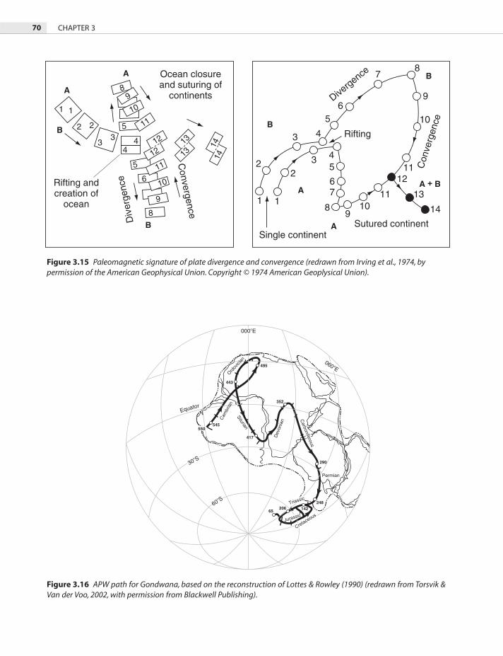
APW paths can be used to interpret motions, collisions, and disruptions of continents (Piper, 1987), and are especially useful for pre-Mesozoic continents whose movements cannot be traced by the pattern of magnetic lineations in their surrounding ocean basins (Section 4.1.6). Figure 3.15 represents the full Wilson cycle (Section 7.9) of the opening and closure of an ocean basin between two continents. Before rifting, the two segments A and B of the initial continent have similar APW paths. They are unlikely to be identical as it is improbable that the initial rift

68 CHAPTER 3

and fi nal suture would coincide. After rifting the two segments describe diverging APW paths until the hairpin at time 8 signals a change in direction of motion to one of convergence. After suturing at time 12 the two segments follow a common polar track.

The southern continents, plus India, are thought to have formed a single continent, Gondwana, from late Pre-Cambrian to mid-Jurassic time. During this period, of approximately 400 Ma, they should have the same polar wander path when reassembled. Figure 3.16 illustrates a modern polar wander path for Gond-wana (Torsvik & Van der Voo, 2002). The track of the path relative to South America can be compared with the very early path given by Creer (1965) (Fig. 3.13b). The seemingly greater detail of the path shown in Fig. 3.16 may however be unwarranted. There is considerable disagreement over the details of the APW path for Gondwana, presumably because of the paucity of suffi cient reliable data (Smith, 1999; McElhinny & McFadden, 2000). Interestingly the path favored by Smith (1999), based on a detailed analysis

of paleomagnetic and paleoclimatic data, is very com-parable to that of Creer (1965). All APW paths for Gondwana have the south pole during Carboniferous times in the vicinity of southeast Africa, as did Wegener (Fig. 1.3), and the Ordovician pole position in northwest Africa, where there is evidence for a minor glaciation in the Saharan region at this time (Eyles, 1993).

3.6.6 Paleogeographic reconstructions based on paleomagnetism

Reconstructions of the relative positions of the main continental areas at various times in the past 200 Ma are best achieved using the very detailed information on the evolution of the present ocean basins pro-vided by the linear oceanic magnetic anomalies

Jurassic

Cambrian

Devonian

Pennsylvanian

Permian

Triassic - Jurassic

Present

Pennsylvanian

Cambrian

L. Permian

Devonian

Figure 3.13 Two methods of displaying paleomagnetic data: (a) assuming fi xed magnetic poles and applying latitudinal shifts to the continent; (b) assuming a fi xed continent and plotting a polar wander path. Subsequent work has modifi ed the detail of the movements shown. Note that the south pole has been plotted (redrawn from Creer, 1965, with permission from the Royal Society of London).

CONTINENTAL DRIFT 69

195

215

235250

215235

255

285

305

345

385 370

435

450

420405

475

195

270

290

315

345450370

385

405

90E 120E 150E 180E

30N

60N

210E

0N

435475

535

500

195

215 235

250

420

450

270290

315

345370

385

40590E 120E 150E 180E

30N

60N

0N

435475

535

500

(a)

(b)

Figure 3.14 Apparent polar wander paths for North America (solid circles and solid line) and Europe (open circles and dashed line) (a) with North America and Europe in their present positions, and (b) after closing the Atlantic ocean. Ages for each mean pole position are given in Ma with those for Europe in italics (redrawn from McElhinny & McFadden, 2000, with permission from Academic Press. Copyright Elsevier 2000).

70 CHAPTER 3

8

6

5

5

1 1

22

3

3

4

4

5

5

6

6

7

7

8

8

9

9

10

10

11

11

12

13

148

10

109

9

11

1212

1313

1414

Rifting andcreation of

ocean

Single continentSutured continent

Rifting

A

A

A

A

A + B

BB

B

B

Ocean closureand suturing of

continents

Div

erge

nce

Divergence

Convergence

Con

verg

ence

43

2 2

11

3 4

11

Figure 3.15 Paleomagnetic signature of plate divergence and convergence (redrawn from Irving et al., 1974, by permission of the American Geophysical Union. Copyright © 1974 American Geoplysical Union).

Equator

Cretaceous

Triassic

Permian

Carboniferous

30�S

60�S

545

417

443

495

352

290

248142206

65

060�E

550

Ordov

ician

Cam

bria

n

Silurian

Dev

onia

n Carboniferous

Permian

Triassic

CretaceousJurassic

000�E

Figure 3.16 APW path for Gondwana, based on the reconstruction of Lottes & Rowley (1990) (redrawn from Torsvik & Van der Voo, 2002, with permission from Blackwell Publishing).

CONTINENTAL DRIFT 71

(Section 4.1.7). In order to position the continents in their correct paleolatitudes however, paleomagnetic results must be combined with these reconstructions to identify the positions of the paleopoles and paleo-equator. The sequence of paleogeographic maps in Chapter 13 (Figs 13.2–13.7) was obtained in this way. For any time prior to 200 Ma the constraints pro-vided by the oceanic data are no longer available and reconstructions are based on paleomagnetic results and geologic correlations. Examples of these pre-Mesozoic reconstructions will be discussed in Chapter 11.

FURTHER READING

Frakes, L.A. (1979) Climates Throughout Geologic Time. Elsevier, New York.

McElhinny, M.W. & McFadden, P.L. (2000) Paleomagnetism: conti-nents and oceans. Academic Press, San Diego.

Tarling, D.H. & Runcorn, S.K. (eds) (1973) Implications of Continen-tal Drift to the Earth Sciences, vols 1 & 2. Academic Press, London.

Tarling, D.H. & Tarling, M.P. (1971) Continental Drift: a study of the Earth’s moving surface. Bell, London.