“Coarse” Notes Population Genetics

VI-1

MIGRATION

ROLES OF MIGRATION IN EVOLUTION READING: Hedrick pp. 403-436.

• Introduces novel genetic variation into populations. • Tends to homogenize gene frequencies in different populations.

• Sets the spatial scale for evolution.

• Opposes local adaptation.

• Migration with an evolutionary impact: Gene Flow

– Migration introduces individuals and genotypes (“dispersal”). – Migrants have no effect on evolution unless their genes are incorporated into a

population.

• A One-Island Model

– The simplest model of migration. – Two alleles A and a. Let p =

frequency of A on island.

– A fraction m of the island gene pool emigrates from the continent where the frequency of A is pc . ⇒ A fraction 1 !m( ) of alleles on

the island originated on the island.

– The continent is too vast to be

influenced by migration from the island ⇒ pc is constant.

– Then the frequency of A on the island changes according to ! p = 1 "m( )p + mpc .

aa

Continent Island

p pcm

“Coarse” Notes Population Genetics

VI-2

– At equilibrium, set ! p = p . • Solving for p gives ˆ p = pc

– Rate of approach to equilibrium:

• Rewrite evolutionary equation as

! p " ˆ p = ! p " pc = 1" m( )p + mpc " pc = 1"m( ) p " pc( )

= 1 "m( ) p " ˆ p ( )

– Conclusions

(1) At equilibrium, both populations have the same allele frequencies. (2) Rate of approach to equilibrium ( ˆ p = pc ) is determined by the migration rate m.

• General Models of Migration – Same conclusions as one-island model hold. – Exceptions, however, do exist

• For example, consider two populations with different allele frequencies that switch locations each generation.

• The populations will obviously

never homogenize (because there's no real exchange of genes).

– Remark: Have implicitly assumed gene frequencies differ in different locations. – How could this be?

– “History.” – Genetic drift. – Selection favors different alleles in different locations.

aa

1 2

m = 1

m = 1

“Coarse” Notes Population Genetics

VI-3

MIGRATION AND DRIFT

• Migration introduces novel genetic variation into local populations. • Drift removes local genetic variation.

Which for dominates?

One answer… • Wright’s “Island Model” • Consider a large number of “islands” each with a population of size N (2N alleles per locus) • Each generation, every island exchanges a

fraction m of its gametes with a ∞-sized “migrant pool” to which all islands contribute gamates.

• Assume infinite-isoalleles model. • Let ft = Pr(pair or randomly drawn gametes

on a typical island are IBD in generation t) = average within-island homozygosity • By the same logic used when studying mutation-drift balance:

!

ft+1 = 1"m( )2 12N

+ 1" 12N

#

$ %

&

' ( f t

)

* +

,

- .

• At equilibrium,

!

ft +1 = f t = ˆ f " 11+ 4Nm

– expression resembles that describing diversity maintained by mutation & drift, with

!

" = 4Nu replaced by 4Nm.

• If 4Nm < 1: Local homozygosity is substantial – drift dominates migration

• If 4Nm > 1: Local diversity (heterozygosity) is substantial – migration dominates drift

Note 1

– 4Nm > 1 same as 2Nm > 1/2

Migrant Pool

…2N 2N 2N 2N 2N

“Coarse” Notes Population Genetics

VI-4

⇒ Migration dominates drift if at least one migrant gamete is exchanged every other generation!

– Conclusion is independent of m, the rate of gene flow. (Why?)

Note 2

– Recall from discussion of F statistics:

!

H S = Avgi

HS,i( ) "1# ˆ f , since

!

ˆ f is the average

local homozygosity and there is no additional inbreeding – Also, HT = 1 – Pr(pair of randomly chosen gametes from entire population are IBD) = 1

– 0 = 1

⇒

!

FST =HT "H S

HT

=1" 1" ˆ f ( )

1= ˆ f =

11+ M

, where M = 4Nm.

– Suggests way to estimate rate of migration from FST:

!

ˆ M = 1" FST

FST

.

– Careful: estimate requires lots of assumptions (island model, equilibrium, etc.) to be

valid. MIGRATION AND SELECTION

• One-island model with selection

– A favored on island. – a fixed on continent: pc = 0. – A is dominant.

• Fitnesses on island:

Genotype AA Aa aa Fitness 1 1 1 ! s

• Life Cycle: zygotes

pselection! " ! ! ! adults

p*

migration! " ! ! ! gametesp**

random union! " ! ! ! ! zygotes# p

• After selection (before migration): p* = p 11 ! q2s

“Coarse” Notes Population Genetics

VI-5

• After migration & reproduction: ! p = 1 "m( )p* + m 0( ) =p 1 "m( )1 " q2s

• To find any equilibria, set ! p = p .

– Solving for p gives ˆ p = 1 ! m s . – Require 0 ! ˆ p ! 1 .

• This occurs only when m < s . • Otherwise ˆ p = 0.

– Now assume A is recessive.

• Fitnesses on island:

Genotype AA Aa aa Fitness 1 1 ! s 1 ! s

• After selection (before migration): p* = p 1! qs( )1! sq 1 + p( )

• After migration & reproduction: ! p = 1 "m( )p* + m 0( ) =p 1 "m( ) 1 " qs( )1" sq 1 + p( )

• To find equilibria, set ! p = p and solve for p.

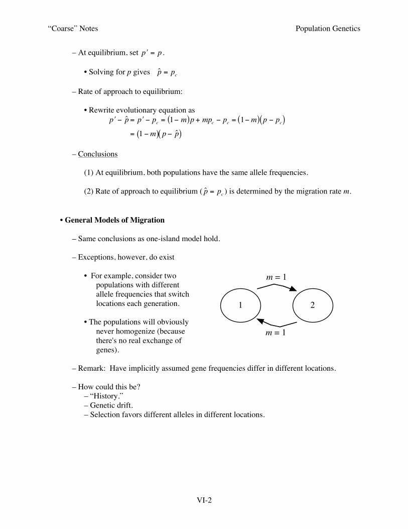
– Get cubic equation for ˆ p 's (up to 3

possible solutions). – ˆ p = 0 is always an equilibrium

(since pc = 0). – There are two polymorphic

equilibria when s > 4m (assuming m is small).

• one equilibrium is stable, the

other is unstable.

– Graphically ⎯⎯⎯⎯⎯⎯→

• Implications

p

ms0

1

0

aa

p

ms/40

stable

unstable

“Coarse” Notes Population Genetics

VI-6

– If recessive selection is strong enough to maintain A in the face of migration, A will spread only if it's initially sufficiently frequent enough. Otherwise, it will be lost.

– In general, unless locally advantageous allele is completely dominant, it must

reach a threshold frequency to persist. – If an allele persists, it won't be found at a low frequency. – Historical "accidents" play a role.

• Identical patches will evolve differently if they differ in initial allele frequency.

• The Levene Model

Q: What happens when a population is made up of a group of distinct subpopulation patches, with different selection pressures occurring in each and migration between locations?

A: Depends on geography (population structure).

– Natural populations fall somewhere between the following two extremes:

• Unrestricted migration.

• Restricted migration.

– A simple model of unrestricted migration was presented in 1953 by H. Levene. – Assumptions of Levene's 1953 model:

• n patches in which different patterns of selection occur.

• Frequency of A among gametes is p. • After fertilization, (diploid) zygotes colonize the different patches (at random).

– Important: this implies that the zygotes within patches are in H-W proportions.

• ith patch makes up a fraction ci of the environment. • Fitnesses in the ith patch:

Genotype AA Aa aa Fitness wAA i( ) wAa i( ) waa i( )

“Coarse” Notes Population Genetics

VI-7

• Random mating between patches.

– Individuals from different localities form a single mating (gamete) pool.

– Why study the Levene model? • Captures essential features of spatially subdivided population and is mathematcially

tractable. • Is a reasonable representation of certain natural systems as well.

– Back to model...How many gametes does each patch contribute to the gamete pool?

• Two extremes:

(1) Hard selection (due to Dempster, 1955) • Patch contributes gametes in proportion to the fraction of survivors.

– i.e., patches with higher fitness contribute disproportionately more.

• Implies population size is not regulated within patches.

(2) Soft selection

• Each patch contributes fixed number of gametes to the mating pool regardless of local fitnesses.

• Number of reproducing adults from each patch is the same from one

generation to the next. • Implies population size is regulated within each patch.

• A schematic comparison

between soft and hard selection, assuming c1 = c2 = c3 = c4 and w 4 > w 3 > w 2 > w 1 ⎯⎯⎯→

– Levene model with hard selection (“constant number of zygotes”): • Assumes contribution of genotype from patch i to the gamete pool is proportional to

it's fitness in that patch [wgenotype i( )] × frequency of i patch in environment (ci ): – i.e., total number of survivors of that genotype in patch i ! ciwgenotype i( )

environment

hard selection

gamete pool

12

34

12

34

environment

soft selection

gamete pool

12

34

12

34

“Coarse” Notes Population Genetics

VI-8

• Overall fitness of genotype in population is its average fitness over patches:

– For example, mean fitness of AA: w AA = ciwAA i( )i=1

n

!

– Likewise for Aa and aa. • Consider changes in the frequency p of A in the gamete pool.

• ! p = p pw AA + qw Aa

w = p w A

w where w A = pw AA + qw Aa and

w = p2w AA + 2pqw Aa + q2w aa .

• Looks just like selection with constant fitnesses: w AA, w Aa ,w aa • Consequences

– An allele will spread if it has the highest arithmetic mean fitness across patches. – Selection will maintain a stable polymorphism if heterozygotes have the

greatest arithmetic mean fitness across patches. • For example, consider two equally sized patches, c1 = c2 = 0.5 .

Fitness in patch: AA Aa aa # 1 0 0.75 1

# 2 1 0.75 0 Average: 0.5 0.75 0.5

• Selection maximizes arithmetic mean fitness across environments

– Levene model with soft selection (“constant number of adults”): – Within each patch, selection operates as usual. – Fitness in patch i: AA Aa aa wi 1 vi – After selection, frequency of A in patch i is

p* i( ) = p pwi + q 1( )p2wi + 2pq 1( ) + q2vi

= p w A i( )w i( )

– Density regulation occurs independently in each patch. – Survivors contribute to gamete pool in proportion to the size (= relative proportion

of adults) of the patch, ci :

“Coarse” Notes Population Genetics

VI-9

! p = cip* i( )

i =1

n

" = ci ppwi + q

p2wi + 2 pq + q2vii =1

n

"

– Equilibrium: set ! p = p and solve for p.

• Results in polynomial of degree 2n +1 in p. ⇒ as many as 2n +1 equilibria, ˆ p , are possible!

• Mathematically too difficult to find all these.

– Alternative: protected polymorphism analysis:

• Near p = 0 , ! p " ci

vi

#

$ %

&

' ( p

i =1

n

) = p 1˜ v

where ˜ v = 1 ci1vi

!

" #

$

% &

i =1

n

'(

) *

+

, - is the harmonic mean fitness of aa homozygotes.

• Note that ! p > p (i.e., !p > 0 ) whenever 1 ˜ v >1! ˜ v < 1

– i.e., whenever the “harmonic mean fitness of aa homozygotes” < “mean fitness of heterozygotes”

• Likewise, near p = 1, (q = 0), ! q > q whenever ˜ w < 1. • Conclude: protected polymorphism occurs with soft selection whenever there is

harmonic mean overdominance in fitness across patches: ˜ w < 1 > ˜ v .

– Bottom line(s) for soft selection • Harmonic mean fitness across patches is the relevant fitness measure if p ≈ 0 or

1. • Turns out, however, that selection maximizes geometric mean fitness.

– Hard versus Soft Selection

• Conditions exist in which an allele will increase under soft selection but not hard

selection. – I.e., polymorphisms can be maintained under a broader range of conditions with

soft selection versus hard selection. – Intuitively follows because under soft selection, individuals compete selectively

only against "patch-mates". • With hard selection, all compete.

“Coarse” Notes Population Genetics

VI-10

– Mathematically follows because harmonic mean is never larger than the

arithmetic mean: ˜ v ! v = civii=1

n

" .

Q: Why does soft selection seem “hard” (density regulation; intense local

competition) while hard selection seems “soft” (little competition; no density regulation)?

A: It all depends on your viewpoint (genetic vs. demographic).

– Soft selection: top 50% in each patch selected.

– Hard selection: top 50% selected (regardless of patch).

# in

divi

dual

s

patch 1 patch 2

body size

# in

divi

dual

s

patch 1 patch 2

body size