Context Meta-Reinforcement Learning via Neuromodulation

Context Meta-Reinforcement Learning via

Neuromodulation

Eseoghene Ben-Iwhiwhua,∗, Jeffery Dicka, Nicholas A. Ketzb, Praveen K.Pillyb, Andrea Soltoggioa

aDepartment of Computer Science, Loughborough University, UKbHRL Laboratories, Malibu, California, US

Abstract

Meta-reinforcement learning (meta-RL) algorithms enable agents to adaptquickly to tasks from few samples in dynamic environments. Such a feat isachieved through dynamic representations in an agent’s policy network (ob-tained via reasoning about task context, model parameter updates, or both).However, obtaining rich dynamic representations for fast adaptation beyondsimple benchmark problems is challenging due to the burden placed on thepolicy network to accommodate different policies. This paper addresses thechallenge by introducing neuromodulation as a modular component to aug-ment a standard policy network that regulates neuronal activities in orderto produce efficient dynamic representations for task adaptation. The pro-posed extension to the policy network is evaluated across multiple discreteand continuous control environments of increasing complexity. To prove thegenerality and benefits of the extension in meta-RL, the neuromodulatednetwork was applied to two state-of-the-art meta-RL algorithms (CAVIAand PEARL). The result demonstrates that meta-RL augmented with neu-romodulation produces significantly better result and richer dynamic repre-sentations in comparison to the baselines.

Keywords: meta-learning, lifelong-learning, deep reinforcement learning,neuromodulation

∗Corresponding authorEmail addresses: [email protected] (Eseoghene Ben-Iwhiwhu),

[email protected] (Jeffery Dick), [email protected] (Nicholas A. Ketz),[email protected] (Praveen K. Pilly), [email protected] (Andrea Soltoggio)

Preprint submitted to Neural Networks November 2, 2021

arX

iv:2

111.

0013

4v1

[cs

.NE

] 3

0 O

ct 2

021

1. Introduction

Human intelligence, though specialized in some sense, is able to gener-ally adapt to new tasks and solve problems from limited experience or fewinteractions. The field of meta-reinforcement learning (meta-RL) seeks toreplicate such a flexible intelligence by designing agents that are capable ofrapidly adapting to tasks from few interactions in an environment. The re-cent progress in the field such as (Rakelly et al., 2019; Finn et al., 2017;Duan et al., 2016b; Wang et al., 2016; Zintgraf et al., 2019; Gupta et al.,2018) have showcased start-of-the-art results. Studies with agents endowedwith such adaptation capabilities are a promising venue for developing muchdesired and needed artificial intelligence systems and robots with lifelonglearning dynamics.

When an agent’s policy for a meta-RL problem is encoded by a neuralnetwork, neural representations are adjusted from a base pre-trained pointto a configuration that is optimal to solve a specific task. Such dynamicrepresentations are a key feature to enable an agent to rapidly adapt todifferent tasks. These representations can be derived from gradient-basedapproaches (Finn et al., 2017), context-based approaches such as memory(Mishra et al., 2018; Wang et al., 2016; Duan et al., 2016b) and probabilistic(Rakelly et al., 2019), or hybrid approaches (i.e., combination of gradient andcontext methods) (Zintgraf et al., 2019). The hybrid approach obtains a taskcontext via gradient updates and thus dynamically alters the representationsof the network. Context approaches such as CAVIA (Zintgraf et al., 2019)and PEARL (Rakelly et al., 2019) are more interpretable as they disentangletask context from the policy network, thus the task context is used to achieveoptimal policies for different tasks.

One limitation of such approaches is that they do not scale well as theproblem complexity increases because of the demand to store many diversepolicies to be reached within a single network. In particular, it is possi-ble that, as tasks grow in complexity, the tasks similarities reduce and thusthe network’s representations required to solve each task optimally becomesdissimilar. We hypothesize that standard policy networks are not likely toproduce diverse policies from a trained base representation because all neu-rons have a homogeneous role or function: thus, significant changes in thepolicy require widespread changes across the network. From this observation,we speculate that a network endowed with modulatory neurons (neuromod-ulators) has a significantly higher ability to modify its policy.

2

Our approach to overcome this limiting design factor in current meta-RLneural approaches is to introduce a neuromodulated policy network to in-crease its ability to encode rich and flexible dynamic representations. Therich representations are measured based on the dissimilarity of the represen-tations across various tasks, and are useful when the optimal policy of anagent (input-to-action mapping) is less similar across tasks. When combinedwith the CAVIA and PEARL meta-learning frameworks, the proposed ap-proach produced better dynamic representations for fast adaptation as theneuromodulators in each layer serve as a means of directly altering the rep-resentations of the layer in addition to the task context.

Several designs exist for neuromodulation (Doya, 2002), either to gateplasticity (Soltoggio et al., 2008; Miconi et al., 2020), gate neural activations(Beaulieu et al., 2020) or alter high level behaviour (Xing et al., 2020). Theproposed mechanism in this work focuses on just one simple principle: mod-ulatory signals alter the representations in each layer by gating the weightedsum of input of the standard neural component.

The primary contribution of this work is a neuromodulated policy networkfor meta-reinforcement learning for solving increasingly difficult problems.The modular approach of the design allows for the proposed layer to be usedwith other existing layers (such as standard fully connected layer, convolu-tional layer and so on) when stacking them to form a deep network. The ex-perimental evidence in this work demonstrates that neuromodulation is ben-eficial to adapt network representations with more flexibility in comparisonto standard networks. Experimental evaluations were conducted across highdimensional discrete and continuous control environments of increasing com-plexity using CAVIA and PEARL meta-RL algorithms. The results indicatethat the neuromodulated networks show an increasing advantage as the prob-lem complexity increases, while they perform comparably on simpler prob-lems. The increased diversity of the representations from the neuromodulatedpolicy network are examined and discussed. The open source implementationof the code can be found at: https://github.com/anon-6994/nm-metarl

2. Related Work

Meta-reinforcement learning. This work builds on the existing metalearning frameworks (Bengio et al., 1992; Schmidhuber et al., 1996; Thrunand Pratt, 1998; Schweighofer and Doya, 2003) in the domain of reinforce-ment learning. Recent studies in meta-reinforcement learning (meta-RL) can

3

https://github.com/anon-6994/nm-metarl

be largely classified into optimization and context-based methods. Optimiza-tion methods (Finn et al., 2017; Li et al., 2017; Stadie et al., 2018; Rothfusset al., 2019) seek to learn good initial parameters of a model that can beadapted with a few gradient steps to a specific task. In contrast, context-based methods seek to adapt a model to a specific task based on few-shotexperiences aggregated into context variables. The context can be derivedvia probabilistic methods (Rakelly et al., 2019; Liu et al., 2021), or recur-rent memory (Duan et al., 2016b; Wang et al., 2016), or recursive networks(Mishra et al., 2018) or the combination of probabilistic and memory (Zint-graf et al., 2020; Humplik et al., 2019). Hybrid methods (Zintgraf et al.,2019; Gupta et al., 2018) combine optimization and context-based methodswhereby task specific context parameters are obtained via gradient updates.

Neuromodulation. Neuromodulation in biological brains is a processwhereby a neuron alters or regulates the properties of other neurons in thebrain (Marder, 2012). The altered properties can either be in the cellularactivities or synaptic weights of the neurons. Well known biological neuro-modulators include dopamine (DA), serotonin (5-HT), acetycholine (ACh),and noradrenaline (NA) (Bear et al., 2020; Avery and Krichmar, 2017). Theneuromodulators were described in Doya (2002) within the reinforcementlearning computation framework, with dopamine loosely mapped to the re-ward signal error (like TD error), serotonin representing discount factor, ace-tycholine representing learning rate and noradrenaline representing random-ness in a policy’s action distribution. Several studies have drawn inspirationfrom neuromodulation and applied it to gradient-based RL (Xing et al., 2020;Miconi et al., 2020) and neuroevolutionary RL (Soltoggio et al., 2007, 2008;Velez and Clune, 2017) for dynamic task settings. In broader machine learn-ing, neuromodulation has been applied to goal-driven perception (Zou et al.,2020), and also in continual learning setting (Beaulieu et al., 2020) where itwas combined with meta-learning to sequentially learn a number of classifi-cation tasks without catastrophic forgetting. The neuromodulators used inthese studies have different designs or functions: plasticity gating (Soltoggioet al., 2008; Miconi et al., 2020), activation gating (Beaulieu et al., 2020),direct action modification in a policy (Xing et al., 2020).

4

3. Background

3.1. Problem Formulation

In a meta-RL setting, there exist a task distribution p(T ) from whichtasks are sampled. Each task Ti is a Markov Decision Process (MDP), whichis a tuple Mi={S,A, q, r, q0} consisting of a state space S, an action space A,a state transition distribution q(st+1|st, at), a reward function r(st, at, st+1),and an initial state distribution q0(s0). When presented with a task Ti, anagent (with a policy represented as π) is required to quickly adapt to thetask from few interactions. Therefore, the goal of the agent for each task it ispresented is to maximize the expected reward in the shortest time possible:

J (π) = Eq0,q,π

[H−1∑t=0

γtr(st, at, st+1)

], (1)

where H is a finite horizon and γ ∈ [0, 1] is the discount factor.

3.2. Context Adaptation via Meta-Learning (CAVIA)

The CAVIA meta-learning framework (Zintgraf et al., 2019) is an exten-sion of the model-agnostic meta-learning algorithm (MAML) (Finn et al.,2017) that is interpretable and less prone to meta-overfitting. The key ideain CAVIA is the introduction of context parameters in a policy network.Therefore, the policy πθ,φ contains the standard network parameters θ andthe context parameters φ. During the adaptation phase for each task (thegradient updates in the inner loop), only the context parameters are updated,while the network parameters are updated during the outer loop gradient up-dates. There are different ways to provide the policy network with the contextparameters. In Zintgraf et al. (2019), the parameters were concatenated tothe input.

In the meta-RL framework, an agent is trained for a number of iterations.For each iteration, N tasks represented as T are sampled from the taskdistribution T . For each task i, a batch of trajectories τ traini is obtainedusing the policy πθ,φ with the context parameters set to an initial conditionφ0. The obtained trajectories for task i are used to perform a one step innerloop gradient update of the context parameters to new values φi, shown inthe equation below:

φi = φ0 − α∇φJTi(τ traini , πθ,φ0), (2)

5

where JTi(τi, πθ,φ) is the objective function for task i. After the one stepgradient update of the policy, another batch of trajectories τ testi is collectedusing the updated task specific policy πθ,φi .

After completing the above procedure for all tasks sampled from T , ameta gradient step (also referred to as the outer loop update) is performed,updating θ to maximize the average performance of the policy across the taskbatch.

θ = θ − β∇θ1

N

∑τi∈T

JTi(τ testi , πθ,φi). (3)

3.3. Probabilistic Embeddings for Actor-Critic Meta-RL (PEARL)

PEARL (Rakelly et al., 2019) is an off-policy meta-RL algorithm thatis based on the soft actor-critic architecture (Haarnoja et al., 2018). Thealgorithm derives the context of the task to which an agent is exposed throughprobabilistic sampling. Given a task, the agent maintains a prior belief ofthe task, and as the agent interacts with the environment, it updates theposterior distribution with goal of identifying the specific task context. Thecontext variables z are concatenated to the input of the actor and critic neuralcomponents of the setup. To estimate this posterior p(z|c), an additionalneural component called an inference network qφ(z|c) is trained using thetrajectories c collected for tasks sampled from the task distribution T . Theobjective function for the actor, critic and inference neural components aredescribed below,

Lactor=Es∼B,a∼πθz∼qφ(z|c)

[DKL

(πθ(a|s, z)

∥∥∥∥exp(Qθ(s, a, z))

Zθ(s)

)](4)

Lcritic = E(s,a,r,s′)∼Bz∼qφ(z|c)

[Qθ(s, a, z)− (r + V (s′, z))]2 (5)

Linference = ET [Ez∼qφ(z|cT )[Lcritic + βDKL(qφ(z|cT )||p(z))]] (6)

where V is a target network and z means that gradients are not beingcomputed through it, p(z) is a unit Gaussian prior over Z, B is the replaybuffer and β is a weighting hyper-parameter.

4. Neuromodulated Network

This section introduces the extension of the policy network with neuro-modulation. A graphical representation of the network is shown in Figure

6

Input

FC 1

FC 2

neuromodulators neuromodulators

NM

1

NM

2

…

(a) Neuromodulated network

gnl+1

h1l+1

h2l

hnl

h1l

g1l+1

hnl+1

h2l+1… …

…

Wg

Ws

Wm

(b) Neuromodulated fully con-nected layer

Figure 1: Overview of the proposed computational framework

1a. The neuromodulated policy network is a stack of neuromodulated fullyconnected layers.

4.1. Computational Framework

A neuromodulated fully connected layer contains two neural components:standard neurons and neuromodulators (see Figure 1b). The standard neu-rons serve as the output of the layer (i.e., the layer’s representations) and theyare connected to the preceding layer via standard fully connected weights W s.The neuromodulators serve as a means to alter the output of the standardneurons. They receive input via standard fully connected weights W g fromthe preceding layer in order to generate their neural activity, which is thenprojected to the standard neurons via another set of fully connected weightsWm. The function of the projected neuromodulatory activity defines the rep-resentation altering mechanism. For example, it could gate the plasticity ofW s, gate neural activation of h or do something else based on the designer’sspecification. While different types of neuromodulators can be used (Doya,2002), in this particular work, we employ an activity-gating neuromodulator.Such neuromodulator multiplies the activity of the target (standard) neuronsbefore a non-linearity is applied to the layer. Formally, the structure can bedescribed with three parameter matrices: W s defines weights connecting theinput to the standard neurons, W g defines weights connecting the input tothe neuromodulators and Wm defines weights connecting the neuromodula-tors to the standard neurons. The step-wise computation of a forward passthrough the neuromodulatory structure is given below:

7

hs = W s · x (7)

g = ReLU(W g · x) (8)

hm = tanh(Wm · g) (9)

h = ReLU(hs ⊗ hm) (10)

where x is the layer’s input, hs is the weighted sum of input of the stan-dard neurons, g is activity of the neuromodulators derived from the weightedsum of input, hm is the neuromodulatory activity projected onto the stan-dard neurons, and h is the output of the layer. The key modulating processtakes place in the element-wise multiplication of the hs and hm.

The tanh non-linearity is employed to enable positive and negative neu-romodulatory signals, and thus gives the network the ability to affect boththe magnitude and the sign of target activation values. When ReLU is usedas the non-linearity for the layer’s output h, hm has the intrinsic ability todynamically turn on or off certain output in h.

A simpler version of the proposed model can be achieved by only consid-ering the sign, and not the magnitude, of the neuromodulatory signal, usingthe following variation of Equation 10:

h = ReLU(hs ⊗ sign(hm)) (11)

This variation is shown to be suited for discrete control problems.A major caveat of the proposed design is that the inclusion of neuro-

modulatory structures into the network increases the number of parameters(hence more memory) and the time complexity of a forward pass throughthe network. However, when only a few neuromodulatory parameters areemployed (in order of hundreds or thousands rather than millions), then theincrease in computational time is negligible.

5. Results and Analysis

In this section, the results of the neuromodulated policy network evalua-tions across high dimensional discrete and continuous control environmentswith varying levels of complexity are presented. The continuous control en-vironments are the simple 2D navigation, the half-cheetah direction (Finn

8

et al., 2017) and velocity (Finn et al., 2017) Mujoco (Todorov et al., 2012)based environments and the meta-world ML1 and ML45 environments (Yuet al., 2020). The discrete action environment is a graph navigation en-vironment that supports configurable levels of complexity called the CT-graph (Soltoggio et al., 2021; Ladosz et al., 2021; Ben-Iwhiwhu et al., 2020).The experimental setup focused on investigating the beneficial effect of theproposed neuromodulatory mechanism when augmenting existing meta-RLframeworks (i.e., neuromodulation as complementary tool to meta-RL ratherthan competing). To this end, using CAVIA meta-RL method (Zintgrafet al., 2019), a standard policy network (SPN) is compared against our neu-romodulated policy network (NPN) across the aforementioned environments.Similarly, SPN is compared against NPN using PEARL (Rakelly et al., 2019)method only in the continuous control environments because the soft actor-critic architecture employed by PEARL is designed for continuous control.We present the analysis of the learned dynamic representations from a stan-dard and a neuromodulated network in Section 5.2. Finally, the policy net-works were evaluated in a RGB autonomous vehicle navigation domain inthe CARLA driving simulator using CAVIA and the results and discussionsare presented in Appendix Appendix E.

5.1. Performance

The experimental setup for CAVIA and PEARL as in Zintgraf et al.(2019) and Rakelly et al. (2019) were followed. For PEARL, neuromodula-tion was applied only to the actor neural component. The details of the ex-perimental setup and hyper-parameters are presented in Appendix AppendixA. The performance reported are the meta-testing results of the agents inthe evaluation environments after meta-training has been completed. Duringmeta-testing in CAVIA, the policy networks were fine-tuned for 4 inner loopgradient steps.

5.1.1. 2D Navigation Environment

The first simulations are in the 2D point navigation experiment intro-duced in Finn et al. (2017). An agent is tasked with navigating to a ran-domly sampled goal position from a start position. A goal position is sampledfrom the interval [-0.5, 0.5]. The reward function is the negative squared dis-tance between the current agent position and the goal. An observation is theagent’s current 2D position while the actions are velocity commands clipped

9

30 20 10 0Average return

SPN

NPN (ours)

2dnavigation

(a) 2D Navigation

100 80 60 40 20 0Average return

SPN

NPN (ours)

halfcheetahvel

(b) Half-Cheetah Velocity

0 100 200 300 400Average return

SPN

NPN (ours)

halfcheetahdir

(c) Half-Cheetah Direction


SPN

NPN (ours)

ml1_push

(d) Meta-World ML1


SPN

NPN (ours)

ml45

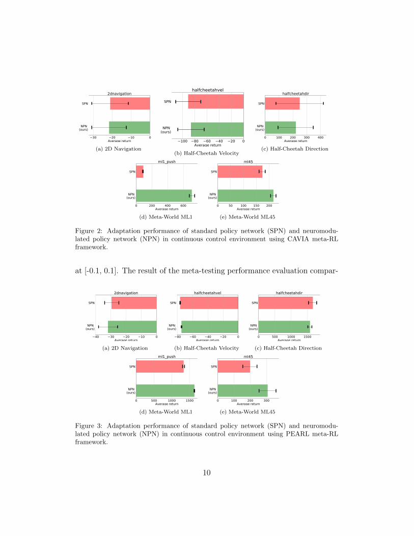
(e) Meta-World ML45

Figure 2: Adaptation performance of standard policy network (SPN) and neuromodu-lated policy network (NPN) in continuous control environment using CAVIA meta-RLframework.

at [-0.1, 0.1]. The result of the meta-testing performance evaluation compar-


SPN

NPN (ours)

2dnavigation

(a) 2D Navigation


SPN

NPN (ours)

halfcheetahvel

(b) Half-Cheetah Velocity


SPN

NPN (ours)

halfcheetahdir

(c) Half-Cheetah Direction


SPN

NPN (ours)

ml1_push

(d) Meta-World ML1


SPN

NPN (ours)

ml45

(e) Meta-World ML45

Figure 3: Adaptation performance of standard policy network (SPN) and neuromodu-lated policy network (NPN) in continuous control environment using PEARL meta-RLframework.

10

0.0 0.1 0.2 0.3Average success rate

SPN

NPN (ours)

ml1_push

(a) CAVIA, ML1

0.00 0.02 0.04 0.06 0.08 0.10Average success rate

SPN

NPN (ours)

ml45

(b) CAVIA, ML45

0.0 0.2 0.4 0.6Average success rate

SPN

NPN (ours)

ml1_push

(c) PEARL, ML1

0.000 0.025 0.050 0.075 0.100 0.125Average success rate

SPN

NPN (ours)

ml45

(d) PEARL, ML45

Figure 4: Adaptation performance (based on success rate metric) of standard policy net-work (SPN) and neuromodulated policy network (NPN) in CAVIA and PEARL.

ing both the standard policy network and neuromodulated policy networkis presented in Figure 2a for CAVIA and Figure 3a for PEARL. The resultshows that both policy networks had a relative good performance. Such opti-mal performance is expected from both policies as the environment is simpleand the dynamic representations required for each task are not very distinct.

5.1.2. Half-Cheetah

The half-cheetah is an environment based on the MuJoCo simulator(Todorov et al., 2012) that requires an agent to learn continuous controllocomotion. We employ two standard meta-RL benchmarks using the envi-ronment as proposed in Finn et al. (2017); (i) the direction task that requiresthe cheetah agent to run either forward or backward and (ii) the velocity taskthat requires the agent to run at a certain velocity sampled from a distri-bution of velocities. Although challenging (due to their high dimensionalnature) in comparison to the 2D navigation task, these benchmark are stillsimplistic as the direction benchmark contains only two unique tasks andthe velocity benchmark samples small range of velocities ([0, 2.0) or [0, 3.0)).Therefore, the optimal policies across tasks in these benchmarks possess sim-ilar representations. The results of the experiments for both benchmarks arepresented in Figures 2c and 2b for CAVIA, and Figures 3c and 3b for PEARL.Unsurprisingly, the results show comparable level of performance betweenthe standard policy network and the neuromodulated policy network acrossCAVIA and PEARL. These benchmarks are of medium complexity and theoptimal policy for each task is similar to others.

5.1.3. Meta-World

The neuromodulated policy network was evaluated in a complex high-dimensional continuous control environment called meta-world (Yu et al.,2020). In meta-world, an agent is required to manipulate a robotic arm to

11

solve a wide range of tasks (e.g. pushing an object, pick and place objects,opening a door and more). Two instances of the benchmark ML1 and ML45were employed. In ML1 instance, the robot is required to solve a single taskthat contains several parametric variations (e.g. push an object to differentgoal locations). The parametric variations of the selected task are used asthe meta-train and meta-test tasks. ML45 is a more complex instance thatcontains a wide variety of tasks (each task with parametric variations). Itconsists of 45 distinct meta-train tasks and 5 distinct meta-test tasks. Thestandard policy network and neuromodulated policy network were evaluatedin ML1 and ML45 instances using CAVIA and PEARL. The results1 arepresented in Figures 2d and 2e for CAVIA, and Figures 3d and 3e for PEARL.In these complex benchmarks, the results show that the neuromodulatedpolicy network outperforms the standard policy network in both CAVIAand PEARL, highlighting the advantage neuromodulation offers in complexproblem setting. In addition to judging the performance based on reward,results are also presented using the success rate metric (introduced in Yuet al. (2020) as a metric judge whether or not an agent is able to solve atask) in Figure 4. The results again show that the neuromodulated policynetwork achieved significantly higher average success rate both in CAVIAand PEARL in comparison to the standard policy network.

5.1.4. Configurable Tree graph (CT-graph) Environment

The CT-graph is a sparse reward discrete control graph environment withincreasing complexity that is specified via parameters such as branch b anddepth d. An environment instance consists of a set of states including a startstate and a number of end states. An agent is tasked with navigating to arandomly sampled end state from the start state. See Appendix Appendix Bfor more details about the CT-graph. The three CT-graph instances used inthis work were setup with varying depth parameter: with increasing depth,the sequence of actions grows linearly, but the search space for the policynetwork grows exponentially. The simplest instance has d set to 2 (CT-graph depth2), and the next has d set to 3 (CT-graph depth3) and the mostcomplex instance has d set to 4 (CT-graph depth4). The meta-testing re-sults are presented in Figure 5. The results show a significant difference in

1The experiments were conducted using the updated Meta-World (i.e., v2) environmentcontaining the updated reward function.

12

0.00 0.25 0.50 0.75 1.00Average return

SPN

NPN (ours)

ctgraph_depth2

(a) CT-graph (b = 2, d = 2)

0.0 0.2 0.4 0.6 0.8 1.0Average return

SPN

NPN (ours)

ctgraph_depth3

(b) CT-graph (b = 2, d = 3)

0.0 0.2 0.4 0.6Average return

SPN

NPN (ours)

ctgraph_depth4

(c) CT-graph (b = 2, d = 4)

Figure 5: Adaptation performance of standard policy network (SPN) and neuromodu-lated policy network (NPN) in three discrete control environments using CAVIA meta-RLframework.

Task1

Task2

Task3

Task4

Task5

Task6

Task6

Task5

Task4

Task3

Task2

Task1

hidden 1, before update

Task1

Task2

Task3

Task4

Task5

Task6

Task6

Task5

Task4

Task3

Task2

Task1

hidden 1, grad 1

Task1

Task2

Task3

Task4

Task5

Task6

Task6

Task5

Task4

Task3

Task2

Task1

hidden 1, grad 2

Task1

Task2

Task3

Task4

Task5

Task6

Task6

Task5

Task4

Task3

Task2

Task1

hidden 1, grad 3

Task1

Task2

Task3

Task4

Task5

Task6

Task6

Task5

Task4

Task3

Task2

Task1

hidden 1, grad 4

0.0 0.2 0.4 0.6 0.8 1.0

(a) standard policy network, first hidden layer.

Task1

Task2

Task3

Task4

Task5

Task6

Task6

Task5

Task4

Task3

Task2

Task1


Task1

Task2

Task3

Task4

Task5

Task6

Task6

Task5

Task4

Task3

Task2

Task1

hidden 1, grad 1

Task1

Task2

Task3

Task4

Task5

Task6

Task6

Task5

Task4

Task3

Task2

Task1

hidden 1, grad 2

Task1

Task2

Task3

Task4

Task5

Task6

Task6

Task5

Task4

Task3

Task2

Task1

hidden 1, grad 3

Task1

Task2

Task3

Task4

Task5

Task6

Task6

Task5

Task4

Task3

Task2

Task1

hidden 1, grad 4

0.0 0.2 0.4 0.6 0.8 1.0

(b) neuromodulated policy network, first hidden layer.

Figure 6: Representation similarities between tasks in the 2D Navigation environment.

performance between standard and neuromodulated policy network. The op-timal adaption performance from the neuromodulated policy network stemsfrom the rich dynamic representations needed for adaptation as discussed inSection 5.2.

5.2. Analysis

In this section, we conduct analysis on the learnt representations of thestandard and neuromodulated policy networks for tasks in the 2D Navigationand CT-graph environments. The policy networks trained using CAVIA waschosen for the analysis as the single neural component in CAVIA (i.e. thepolicy network) makes it easier to analyse in comparison to PEARL whichcontain multiple neural components.

13

Task1 Task2 Task3 Task4

Task4

Task3

Task2

Task1



Task4

Task3

Task2

Task1

hidden 1, grad 1


Task4

Task3

Task2

Task1

hidden 1, grad 2


Task4

Task3

Task2

Task1

hidden 1, grad 3


Task4

Task3

Task2

Task1

hidden 1, grad 4

0.0 0.2 0.4 0.6 0.8 1.0



Task4

Task3

Task2

Task1



Task4

Task3

Task2

Task1

hidden 1, grad 1


Task4

Task3

Task2

Task1

hidden 1, grad 2


Task4

Task3

Task2

Task1

hidden 1, grad 3


Task4

Task3

Task2

Task1

hidden 1, grad 4

0.0 0.2 0.4 0.6 0.8 1.0

(b) neuromodulated policy network, first hidden layer.

Figure 7: Representation similarities between tasks in the CT-graph depth2 environment.

To measure representation similarity across task, we employ the use ofthe central kernel alignment (CKA) (Kornblith et al., 2019) similarity index,comparing per layer representations of both standard and neuromodulatedpolicy networks across different tasks. The representation similarities be-tween tasks were plotted as heat maps in Figure 6 and 7. Each heatmapin a row (for example 6a) depict the similarity before or after few steps ofgradient updates to the layer. Before any gradient updates, the representa-tions are similar between tasks in the figure. After gradient updates, somedissimilarities between tasks begin to emerge. Additional analysis plots arepresented in Appendix Appendix C.

2D Navigation. For the simple 2D Navigation environment, the plotsfor the first hidden layer of the standard policy network shown in Figure6a depicts good dissimilarity between tasks, thus highlighting the fact thatthe learnt representations are sufficient enough to produce distinct task be-haviours. The same is true as well for the first hidden layer of the neuromod-ulated policy network (see Figure 6b). This further justifies why both policiesobtained roughly comparable performance in this environment. The simplic-ity of the problem enables task distinct representations to be obtained easily.Appendix Appendix C.1 contains the plots of the representation similarityfor the second hidden layer of both policy networks.

CT-graph. In Figure 7a and 7b, we compare the representation simi-larity of the first hidden layer of the standard and neuromodulated policynetworks in the CT-graph depth2 environment. We see that representations

14

of the neuromodulated policy are more dissimilar between the tasks thanthose of the standard policy. Due to the complexity of the environment,the task specific representations required to solve each task are distinct fromone another. Therefore, adaptation by fine-tuning the representations of abase network via few gradient steps of parameters update would require asignificant jump in the solution space. Standard policy network struggles toenable such jump in the solution space. However, by incorporating neuro-modulators that dynamically alters the representations, such jump becomespossible. Appendix Appendix C.1 contains the plots of the representationsimilarity for the second hidden layer of both policy networks.

5.3. Control Experiments: with equal number of parameters

0.0 0.1 0.2 0.3 0.4 0.5 0.6 0.7Average return

SPN

SPN (larger)

NPN (ours)

ctgraph_depth4_control_experiment

(a) CT-graph depth4


SPN

SPN (larger)

NPN (ours)

ml45_control_experiment

(b) ML45

Figure 8: Control experiments. Adaptation performance of standard policy network(SPN), a larger SPN variant and neuromodulated policy network (NPN) using CAVIA.Note, the number of parameters in SPN (larger) approximately matches that of the NPNin each environment.

Since the inclusion of neuromodulators increases the number of parame-ters in a neuromodulated policy network, a set of control experiments wereconducted in which the number of parameters in a standard policy networkwas configured to approximately match that of a neuromodulated policy net-work. This was achieved by increasing the size of each hidden layers in thestandard policy network. Using CAVIA, experiments were conducted in theCT-graph depth4 and the ML45 meta-world environments, comparing thestandard policy network (i.e., the original size), its larger variant and a neu-romodulated policy network. The results are presented in Figure 8. Weobserve from the results that the increase in the size of the policy network

15

does not lead to match of the performance of the neuromodulated policynetwork.

6. Discussions

Neuromodulation and gated recurrent networks: The neuromodu-latory gating mechanism introduced in this work is reminiscent of the gatingin recurrent/memory networks (LSTMs (Hochreiter and Schmidhuber, 1997)and GRUs (Cho et al., 2014)). In this respect (with the observation ofimproved performance as a consequence of neuromodulatory gating in thiswork), the noteworthy performance demonstrated by meta-RL memory ap-proaches (Duan et al., 2016b; Wang et al., 2016) could also be a consequenceof such gating mechanisms2. Nonetheless, the present study aims to highlightthe advantage of a simpler form of gating (i.e., neuromodulatory gating) on aMLP feedforward network, and thus could help to pinpoint the advantage ofsuch dynamics in isolation. Furthermore, the advantage of our approach overgated recurrent variants is somewhat similar to the advantages derived fromdecoupling attention mechanism from recurrent models (where it was origi-nally introduced) and applying it to MLP networks (i.e., Transformer models)(Vaswani et al., 2017). By decoupling neuromodulatory (gating) mechanismfrom recurrent models and applying it to MLP models (as in our work), theadvantages of faster training and better parallelization were achieved whilemaintaining the benefit of neuromodulatory gating. Therefore, our proposedapproach is faster to train and more parallelizable in comparison to mem-ory variants, while maintaining the advantages that neuromodulatory gatingoffers. Memory based approaches will still be required for problems wherememory is advantageous such as sequential data processing and POMDPs.

Task similarity measure and robust benchmarks: Increasing taskcomplexity was presented in this work by moving from simple 2D point nav-igation environment to half-cheetah locomotion and then to the complexrobotic arm setup of the Meta-World environment. Furthermore, exploit-ing the benefits of configurable parameters in the CT-graph environment,we were able to control the complexity in the environment. Overall, task

2Although not the focus of this work, we ran an experiment using RL2 (a memory basedmeta-RL method) in the ML45 environment and achieved an average meta-test success rateperformance of 10%, which is comparable to the results obtained using neuromodulatorygating mechanism.

16

complexity was viewed through the perspective of task similarity (i.e., envi-ronments with dissimilar task were viewed as more complex and vice versa).Despite these efforts, a precise measure of task complexity and similaritywas not clearly outlined in this work and this is widely the case in meta-RLliteratures. There is a need for the development of precise metrics for mea-suring task similarity and complexity in the field. The CT-graph with itsconfigurable parameters allow for tasks to be mathematically defined, whichis a first step towards alleviating this issue. However, a separate future re-search investigation would be necessary to develop explicit metrics that canbe incorporated into meta-RL benchmarks.

We hypothesize that such a task similarity metric should be able to cap-ture the precise change points in a task relative to other tasks. For example,a useful metric could be one that capture task change either as a functionof change in reward, or state space, or transition function, or a combina-tion of these factors. Most benchmarks in meta-RL have been focused ontask change as reward function change. However, a more robust benchmarkcould include the aforementioned change points in order to further control thecomplexity. The CT-graph, Meta-world, and the recently developed Alchemy(Wang et al., 2021) environment are examples of benchmarks with early stagework in this direction, albeit implicitly. Therefore, the development of a pre-cise measure of task similarity and complexity, as well as robust benchmarkswith configurable change points (i.e., reward, state/input, and transition)would be highly beneficial to the meta-RL field.

7. Conclusion and Future Work

This paper introduced an architectural extension of the standard meta-RL policy networks to include a neuromodulatory mechanism, investigatingthe beneficial effect of neuromodulation when augmenting existing meta-RLframeworks (i.e., neuromodulation as complementary tool to meta-RL ratherthan competing). The aim is to implement richer dynamic representationsand facilitate rapid task adaptation in increasingly complex problems. Theeffectiveness of the proposed approach was evaluated in meta-RL settingusing CAVIA and PEARL algorithms. In the experimental setup acrossenvironments of increasing complexity, the neuromodulated policy networksignificantly outperformed the standard policy network in complex problemswhile showcasing comparable performance in simpler problems. The resultshighlight the usefulness of neuromodulators to enable fast adaptation via

17

rich dynamic representations in meta-RL problems. The architectural exten-sion, although simple, presents a general framework for extending meta-RLpolicy networks with neuromodulators that expand their ability to encodedifferent policies. The projected neuromodulatory activity can be designedto perform other functions apart from the one introduced in this work e.g.,gating plasticity of weights, or including different neuromodulators in thesame layer. The neuromodulatory extension could also be tested with a re-current meta-RL policy, with the goal of enhancing the memory dynamics ofthe policy.

18

Supplementary Material

Appendix A. Experimental Configurations

All experiments were conducted using machines containing Tesla K80 andGeForce RTX 2080 GPUs. Also note that across all experiments, the outputlayer in the neuromodulated policy network (in CAVIA and in PEARL)employed a regular fully connected linear layer while the preceding layerswere neuromodulated fully connected layers.

Appendix A.1. CAVIA

Following the experimental setup of the original CAVIA paper (Zintgrafet al., 2019), the context variables were concatenated to the input of thepolicy network and were reset to zero at the beginning of each task acrossall experiments. Also, during each training iteration, the policy was adaptedusing one gradient update in the inner loop as employed in Zintgraf et al.(2019); Finn et al. (2017). After training, the iteration with the best policyperformance or the final policy at the end of training was used to conductmeta-testing evaluations to produce the final result. During meta-testing,the policy was evaluated using a number of tasks sampled from the taskdistribution and it was adapted (fine-tuned) for each task using 4 inner loopgradient updates. All policy networks employed ReLU non-linearity acrossall experiments.

The CAVIA experimental configurations across all environments are pre-sented in Table A.1, with 2D Nav denoting the 2D navigation benchmark,Ch Dir and Ch Vel denoting the Half-Cheetah direction and Half-CheetahVelocity benchmarks, ML 1 and ML45 denoting the meta-world ML1 andML45 benchmarks, CT d2, d3, d4 denoting the CT-graph depth2, 3 and 4benchmarks respectively.

Across all experiments in CAVIA, Trust Region Policy Optimization(TRPO) (Schulman et al., 2015) was employed as the outer loop updatealgorithm. Vanilla policy gradient (Williams, 1992) with generalized advan-tage estimation (GAE) (Schulman et al., 2016) was employed as the innerloop update algorithm with learning rate of 0.5 for the 2D navigation andthe CT-graph experiments, and 10.0 for half-cheetah and meta-world exper-iments. Both the inner and outer loop training employed a linear featurebaseline introduced in Duan et al. (2016a). The hyperparameters for TRPOare presented in Table A.2. Furthermore, finite-differences was employed to

19

2DNav

ChDir

ChVel

ML1

ML45

CTd2

CTd3

CTd4

Number of iterations500 500 500 500 500 500 700 1500

Number tasks per iteration(meta-batch size)

20 40 40 40 45 20 25 20

Number inner loop gradsteps(for meta-training)

1 1 1 1 1 1 1 1

Number trajectories pertask(for meta-training)

20 20 20 20 10 20 25 60

Number inner loop gradsteps(for meta-testing)

4 4 4 4 4 4 4 4

Number trajectories pertask(for meta-testing)

20 40 40 40 20 20 40 100

Policy network specifi-cation

Number of context parame-ters

5 50 50 50 100 5 10 20

Number of hidden layers2 2 2 2 2 2 2 2

Hidden layer size100 200 200 200 200 200 300 600

Neuromodulator size (forneuromodulated policyonly)

4 32 32 32 32 8 16 32

Table A.1: CAVIA experimental configurations.

compute the Hessian-vector product for TRPO in order to avoid computingthird-order derivatives as highlighted in Finn et al. (2017). During samplingof data for each task in environments, multiprocessing was employed using 4

20

D

D

S W D

W

W

G

EW

W E

W

W E

C

BA

start wait decision end end (goal location)

D

D

S W D

W

W

E

E

W

W

E

W

W

G

C

D

D

D

D

W

W

W

W

W

W

W

W

E

E

E

E

CT-graph

crash

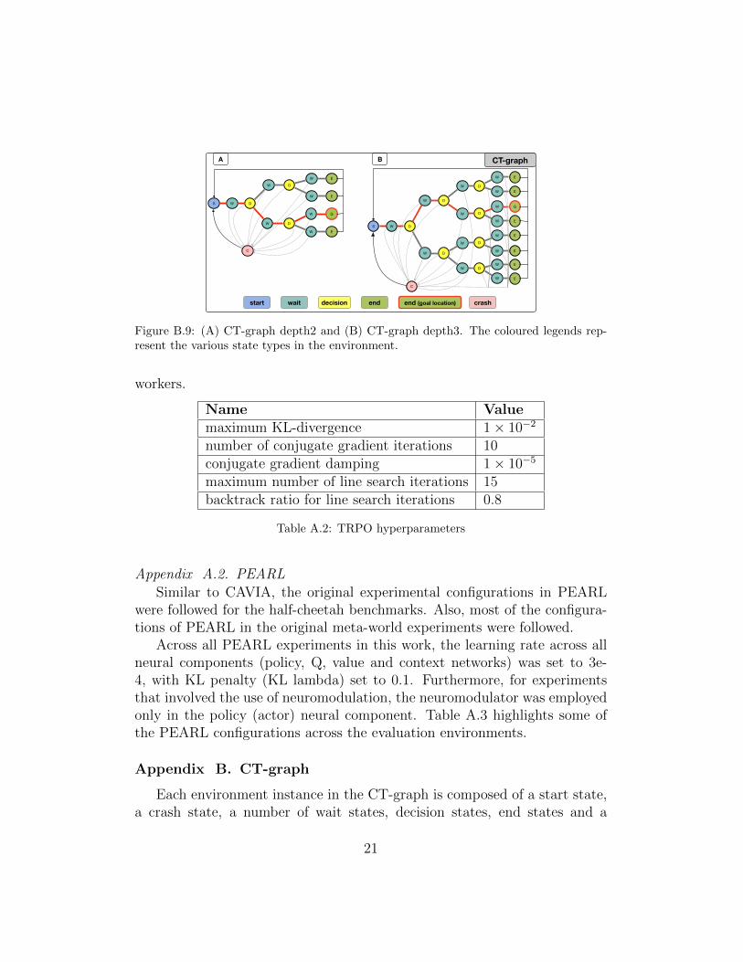
Figure B.9: (A) CT-graph depth2 and (B) CT-graph depth3. The coloured legends rep-resent the various state types in the environment.

workers.

Name Valuemaximum KL-divergence 1× 10−2

number of conjugate gradient iterations 10conjugate gradient damping 1× 10−5

maximum number of line search iterations 15backtrack ratio for line search iterations 0.8

Table A.2: TRPO hyperparameters

Appendix A.2. PEARL

Similar to CAVIA, the original experimental configurations in PEARLwere followed for the half-cheetah benchmarks. Also, most of the configura-tions of PEARL in the original meta-world experiments were followed.

Across all PEARL experiments in this work, the learning rate across allneural components (policy, Q, value and context networks) was set to 3e-4, with KL penalty (KL lambda) set to 0.1. Furthermore, for experimentsthat involved the use of neuromodulation, the neuromodulator was employedonly in the policy (actor) neural component. Table A.3 highlights some ofthe PEARL configurations across the evaluation environments.

Appendix B. CT-graph

Each environment instance in the CT-graph is composed of a start state,a crash state, a number of wait states, decision states, end states and a

21

2DNav

ChDir

ChVel

ML 1ML45

Number of iterations500 500 500 1000 1000

Number of train task40 2 100 50 225

Number of test task40 2 30 50 25

Number of initial steps1000 2000 2000 4000 4000

Number of steps prior400 1000 400 750 750

Number of steps posterior0 0 0 0 0

Number of extra posterior steps600 1000 600 750 750

Reward scale5 5 5 10 5

Policy network specification

Context vector size5 5 5 7 7

Network size(policy, Q and value networks)

300 300 300 300 300

Inference (context) network size200 200 200 200 200

Number of hidden layers (policy, Q,value and context networks)

3 3 3 3 3

Neuromodulator size(for neuromodulated policy only)

4 32 32 32 32

Table A.3: PEARL experimental configurations.

goal state (one of the end states designated as the goal). A wait state isfound between decision states (the tree graph splits at decision states). Thewait state requires an agent to take a wait (forward) action, a decision state

22

requires an agent to take one of the decision (turn) actions. Any decisionaction at a wait state, or wait action at a decision state leads to a crashwhere the agent is punished with a negative reward of -0.01 and returnsto the start. When an agent navigates to the correct end state (the goallocation), it receives a positive reward of 1.0. Otherwise, the agent receives areward of 0.0 at every time step. An episode is terminated either at a crashstate or when the agent navigates to any end state. The observations are1D vector (with full observability of each state) whose length depends on theenvironment instance configuration.

The environment’s complexity is defined via a number of configurationparameters that is used to specify the graph size (using branch b and d),sequence length, reward function, and level of state observability. The threeCT-graph instances used in this work were setup with varying depth param-eter. The simplest instance has d set to 2 (CT-graph depth2), and the nexthas d set to 3 (CT-graph depth3) and the most complex instance has d setto 4 (CT-graph depth4). Figure B.9 depicts a graphical view of CT-graphdepth2 and 3.

Appendix C. Analysis Plots

This section presents additional analysis plots of the representation sim-ilarity across tasks for the standard and neuromodulated policy networksin the various evaluation environments employed in this work. The addi-tional plots further highlights the usefulness of neuromodulation to facilitateefficient (distinct) representations across tasks in problems of increasing com-plexity as earlier showcased in Section 5.2.

Appendix C.1. Second hidden layer: 2D Navigation and CT-graph depth2environments

2D Navigation: Figure C.10 present the representation similarity be-tween tasks, across inner loop gradient updates for the second hidden layerof both policy networks in the 2D navigation environment. Again, similarpatterns as highlighted in the first hidden layer of the policy networks inFigure 6 emerge. Both networks are able to learn good (dissimilar) repre-sentations between tasks after few steps of inner loop gradient update. Also,both networks, before any gradient update, already have some level of rep-resentation disimilarity between tasks. Thus, this further highlights the fact

23

Task1

Task2

Task3

Task4

Task5

Task6

Task6

Task5

Task4

Task3

Task2

Task1


Task1

Task2

Task3

Task4

Task5

Task6

Task6

Task5

Task4

Task3

Task2

Task1

hidden 2, grad 1

Task1

Task2

Task3

Task4

Task5

Task6

Task6

Task5

Task4

Task3

Task2

Task1

hidden 2, grad 2

Task1

Task2

Task3

Task4

Task5

Task6

Task6

Task5

Task4

Task3

Task2

Task1

hidden 2, grad 3

Task1

Task2

Task3

Task4

Task5

Task6

Task6

Task5

Task4

Task3

Task2

Task1

hidden 2, grad 4

0.0 0.2 0.4 0.6 0.8 1.0

(a) standard policy network, second hidden layer.

Task1

Task2

Task3

Task4

Task5

Task6

Task6

Task5

Task4

Task3

Task2

Task1


Task1

Task2

Task3

Task4

Task5

Task6

Task6

Task5

Task4

Task3

Task2

Task1

hidden 2, grad 1

Task1

Task2

Task3

Task4

Task5

Task6

Task6

Task5

Task4

Task3

Task2

Task1

hidden 2, grad 2

Task1

Task2

Task3

Task4

Task5

Task6

Task6

Task5

Task4

Task3

Task2

Task1

hidden 2, grad 3

Task1

Task2

Task3

Task4

Task5

Task6

Task6

Task5

Task4

Task3

Task2

Task1

hidden 2, grad 4

0.0 0.2 0.4 0.6 0.8 1.0

(b) neuromodulated policy network, second hidden layer.

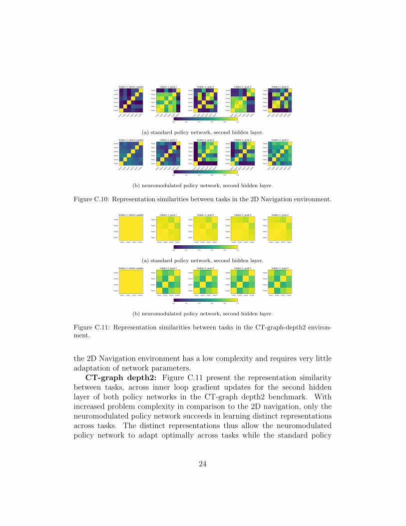
Figure C.10: Representation similarities between tasks in the 2D Navigation environment.


Task4

Task3

Task2

Task1



Task4

Task3

Task2

Task1

hidden 2, grad 1


Task4

Task3

Task2

Task1

hidden 2, grad 2


Task4

Task3

Task2

Task1

hidden 2, grad 3


Task4

Task3

Task2

Task1

hidden 2, grad 4

0.0 0.2 0.4 0.6 0.8 1.0

(a) standard policy network, second hidden layer.


Task4

Task3

Task2

Task1



Task4

Task3

Task2

Task1

hidden 2, grad 1


Task4

Task3

Task2

Task1

hidden 2, grad 2


Task4

Task3

Task2

Task1

hidden 2, grad 3


Task4

Task3

Task2

Task1

hidden 2, grad 4

0.0 0.2 0.4 0.6 0.8 1.0

(b) neuromodulated policy network, second hidden layer.

Figure C.11: Representation similarities between tasks in the CT-graph-depth2 environ-ment.

the 2D Navigation environment has a low complexity and requires very littleadaptation of network parameters.

CT-graph depth2: Figure C.11 present the representation similaritybetween tasks, across inner loop gradient updates for the second hiddenlayer of both policy networks in the CT-graph depth2 benchmark. Withincreased problem complexity in comparison to the 2D navigation, only theneuromodulated policy network succeeds in learning distinct representationsacross tasks. The distinct representations thus allow the neuromodulatedpolicy network to adapt optimally across tasks while the standard policy

24

network struggles, as indicated by the performance plot in Figure 5a.

Appendix C.2. CT-graph depth3 and depth4 Environments

Task1

Task2

Task3

Task4

Task5

Task6

Task7

Task8

Task8Task7Task6Task5Task4Task3Task2Task1


Task1

Task2

Task3

Task4

Task5

Task6

Task7

Task8


hidden 1, grad 1

Task1

Task2

Task3

Task4

Task5

Task6

Task7

Task8


hidden 1, grad 2

Task1

Task2

Task3

Task4

Task5

Task6

Task7

Task8


hidden 1, grad 3

Task1

Task2

Task3

Task4

Task5

Task6

Task7

Task8


hidden 1, grad 4

0.0 0.2 0.4 0.6 0.8 1.0


Task1

Task2

Task3

Task4

Task5

Task6

Task7

Task8



Task1

Task2

Task3

Task4

Task5

Task6

Task7

Task8


hidden 2, grad 1

Task1

Task2

Task3

Task4

Task5

Task6

Task7

Task8


hidden 2, grad 2

Task1

Task2

Task3

Task4

Task5

Task6

Task7

Task8


hidden 2, grad 3

Task1

Task2

Task3

Task4

Task5

Task6

Task7

Task8


hidden 2, grad 4

0.0 0.2 0.4 0.6 0.8 1.0

(b) standard policy network, second hidden layer.

Task1

Task2

Task3

Task4

Task5

Task6

Task7

Task8



Task1

Task2

Task3

Task4

Task5

Task6

Task7

Task8


hidden 1, grad 1

Task1

Task2

Task3

Task4

Task5

Task6

Task7

Task8


hidden 1, grad 2

Task1

Task2

Task3

Task4

Task5

Task6

Task7

Task8


hidden 1, grad 3

Task1

Task2

Task3

Task4

Task5

Task6

Task7

Task8


hidden 1, grad 4

0.0 0.2 0.4 0.6 0.8 1.0

(c) neuromodulated policy network, first hidden layer.

Task1

Task2

Task3

Task4

Task5

Task6

Task7

Task8



Task1

Task2

Task3

Task4

Task5

Task6

Task7

Task8


hidden 2, grad 1

Task1

Task2

Task3

Task4

Task5

Task6

Task7

Task8


hidden 2, grad 2

Task1

Task2

Task3

Task4

Task5

Task6

Task7

Task8


hidden 2, grad 3

Task1

Task2

Task3

Task4

Task5

Task6

Task7

Task8


hidden 2, grad 4

0.0 0.2 0.4 0.6 0.8 1.0

(d) neuromodulated policy network, second hidden layer.

Figure C.12: Representation similarities between tasks in the CT-graph depth3 environ-ment.

The representation similarity plots (across inner loop gradient updates)between tasks of the hidden layers of both the standard and the neuromod-ulated policy networks in the CT-graph depth3 and depth4 environment in-stances are presented in Figure C.12 and C.13. Again, as observed in Section5.2, the standard policy network still struggles to learn distinct representa-tions for each task, whereas, the neuromodulated policy network is able tolearn the required task-specific representations. Hence, the neuromodulatedpolicy network is able to perform optimally across tasks. This explains thedifference in performance (Figures 5b and 5c) between the policy networks.

25

Task1

Task2

Task3

Task4

Task5

Task6

Task7

Task8



Task1

Task2

Task3

Task4

Task5

Task6

Task7

Task8


hidden 1, grad 1

Task1

Task2

Task3

Task4

Task5

Task6

Task7

Task8


hidden 1, grad 2

Task1

Task2

Task3

Task4

Task5

Task6

Task7

Task8


hidden 1, grad 3

Task1

Task2

Task3

Task4

Task5

Task6

Task7

Task8


hidden 1, grad 4

0.0 0.2 0.4 0.6 0.8 1.0


Task1

Task2

Task3

Task4

Task5

Task6

Task7

Task8



Task1

Task2

Task3

Task4

Task5

Task6

Task7

Task8


hidden 2, grad 1

Task1

Task2

Task3

Task4

Task5

Task6

Task7

Task8


hidden 2, grad 2

Task1

Task2

Task3

Task4

Task5

Task6

Task7

Task8


hidden 2, grad 3

Task1

Task2

Task3

Task4

Task5

Task6

Task7

Task8


hidden 2, grad 4

0.0 0.2 0.4 0.6 0.8 1.0


Task1

Task2

Task3

Task4

Task5

Task6

Task7

Task8



Task1

Task2

Task3

Task4

Task5

Task6

Task7

Task8


hidden 1, grad 1

Task1

Task2

Task3

Task4

Task5

Task6

Task7

Task8


hidden 1, grad 2

Task1

Task2

Task3

Task4

Task5

Task6

Task7

Task8


hidden 1, grad 3

Task1

Task2

Task3

Task4

Task5

Task6

Task7

Task8


hidden 1, grad 4

0.0 0.2 0.4 0.6 0.8 1.0


Task1

Task2

Task3

Task4

Task5

Task6

Task7

Task8



Task1

Task2

Task3

Task4

Task5

Task6

Task7

Task8


hidden 2, grad 1

Task1

Task2

Task3

Task4

Task5

Task6

Task7

Task8


hidden 2, grad 2

Task1

Task2

Task3

Task4

Task5

Task6

Task7

Task8


hidden 2, grad 3

Task1

Task2

Task3

Task4

Task5

Task6

Task7

Task8


hidden 2, grad 4

0.0 0.2 0.4 0.6 0.8 1.0


Figure C.13: Representation similarities between tasks in the CT-graph depth4 environ-ment.

Appendix C.3. Half-Cheetah and Meta-World Environments

The CAVIA policies analysis plots for the half-cheetah and meta-worldbenchmarks are presented in this section.

Half-Cheetah: Figure C.14 and C.15 shows the representation sim-ilarity plots of the standard and neuromodulated policy networks for theHalf-Cheetah direction and velocity environments respectively. In this set-ting where the problems are of simple to medium complexity, both policynetworks are able to learn efficient (dissimilar) representations between tasks,further buttressing the discussions in Section 5.2. In fact, we observe thatthe standard policy network learns better dissimilar representations acrosstasks for the half-cheetah direction environment due to the simplicity of thetasks in the environment in comparison to the velocity environment.

Meta-World: Also, Figure C.16 and C.17 depicts the representationsimilarity plots for the ML1 and ML45 meta-world environment. Similarto the observations in Section 5.2, we observe again that as the problem

26

Task1

Task2

Task3

Task4

Task5

Task6

Task6

Task5

Task4

Task3

Task2

Task1


Task1

Task2

Task3

Task4

Task5

Task6

Task6

Task5

Task4

Task3

Task2

Task1

hidden 1, grad 1

Task1

Task2

Task3

Task4

Task5

Task6

Task6

Task5

Task4

Task3

Task2

Task1

hidden 1, grad 2

Task1

Task2

Task3

Task4

Task5

Task6

Task6

Task5

Task4

Task3

Task2

Task1

hidden 1, grad 3

Task1

Task2

Task3

Task4

Task5

Task6

Task6

Task5

Task4

Task3

Task2

Task1

hidden 1, grad 4

0.0 0.2 0.4 0.6 0.8 1.0


Task1

Task2

Task3

Task4

Task5

Task6

Task6

Task5

Task4

Task3

Task2

Task1


Task1

Task2

Task3

Task4

Task5

Task6

Task6

Task5

Task4

Task3

Task2

Task1

hidden 2, grad 1

Task1

Task2

Task3

Task4

Task5

Task6

Task6

Task5

Task4

Task3

Task2

Task1

hidden 2, grad 2

Task1

Task2

Task3

Task4

Task5

Task6

Task6

Task5

Task4

Task3

Task2

Task1

hidden 2, grad 3

Task1

Task2

Task3

Task4

Task5

Task6

Task6

Task5

Task4

Task3

Task2

Task1

hidden 2, grad 4

0.0 0.2 0.4 0.6 0.8 1.0


Task1

Task2

Task3

Task4

Task5

Task6

Task6

Task5

Task4

Task3

Task2

Task1


Task1

Task2

Task3

Task4

Task5

Task6

Task6

Task5

Task4

Task3

Task2

Task1

hidden 1, grad 1

Task1

Task2

Task3

Task4

Task5

Task6

Task6

Task5

Task4

Task3

Task2

Task1

hidden 1, grad 2

Task1

Task2

Task3

Task4

Task5

Task6

Task6

Task5

Task4

Task3

Task2

Task1

hidden 1, grad 3

Task1

Task2

Task3

Task4

Task5

Task6

Task6

Task5

Task4

Task3

Task2

Task1

hidden 1, grad 4

0.0 0.2 0.4 0.6 0.8 1.0


Task1

Task2

Task3

Task4

Task5

Task6

Task6

Task5

Task4

Task3

Task2

Task1


Task1

Task2

Task3

Task4

Task5

Task6

Task6

Task5

Task4

Task3

Task2

Task1

hidden 2, grad 1

Task1

Task2

Task3

Task4

Task5

Task6

Task6

Task5

Task4

Task3

Task2

Task1

hidden 2, grad 2

Task1

Task2

Task3

Task4

Task5

Task6

Task6

Task5

Task4

Task3

Task2

Task1

hidden 2, grad 3

Task1

Task2

Task3

Task4

Task5

Task6

Task6

Task5

Task4

Task3

Task2

Task1

hidden 2, grad 4

0.0 0.2 0.4 0.6 0.8 1.0


Figure C.14: Representation similarities between tasks in the Half-Cheetah Direction en-vironment.

complexity increase (i.e., from ML1 to ML45), the neuromodulated policynetwork produces better (dissimilar) representations across the sampled tasksin comparison to the standard policy network.

Appendix D. Implementation

A code snippet demonstrating the extension of the fully connected layerwith neuromodulation is presented below using PyTorch code style.

class NMLinear(Module):

def __init__(self, in_features, out_features, nm_features, bias=True,

gate=None):

super(NMLinear, self).__init__()

self.in_features = in_features

self.out_features = out_features

self.nm_features = nm_features

27

Task1

Task2

Task3

Task4

Task5

Task6

Task6

Task5

Task4

Task3

Task2

Task1


Task1

Task2

Task3

Task4

Task5

Task6

Task6

Task5

Task4

Task3

Task2

Task1

hidden 1, grad 1

Task1

Task2

Task3

Task4

Task5

Task6

Task6

Task5

Task4

Task3

Task2

Task1

hidden 1, grad 2

Task1

Task2

Task3

Task4

Task5

Task6

Task6

Task5

Task4

Task3

Task2

Task1

hidden 1, grad 3

Task1

Task2

Task3

Task4

Task5

Task6

Task6

Task5

Task4

Task3

Task2

Task1

hidden 1, grad 4

0.0 0.2 0.4 0.6 0.8 1.0


Task1

Task2

Task3

Task4

Task5

Task6

Task6

Task5

Task4

Task3

Task2

Task1


Task1

Task2

Task3

Task4

Task5

Task6

Task6

Task5

Task4

Task3

Task2

Task1

hidden 2, grad 1

Task1

Task2

Task3

Task4

Task5

Task6

Task6

Task5

Task4

Task3

Task2

Task1

hidden 2, grad 2

Task1

Task2

Task3

Task4

Task5

Task6

Task6

Task5

Task4

Task3

Task2

Task1

hidden 2, grad 3

Task1

Task2

Task3

Task4

Task5

Task6

Task6

Task5

Task4

Task3

Task2

Task1

hidden 2, grad 4

0.0 0.2 0.4 0.6 0.8 1.0


Task1

Task2

Task3

Task4

Task5

Task6

Task6

Task5

Task4

Task3

Task2

Task1


Task1

Task2

Task3

Task4

Task5

Task6

Task6

Task5

Task4

Task3

Task2

Task1

hidden 1, grad 1

Task1

Task2

Task3

Task4

Task5

Task6

Task6

Task5

Task4

Task3

Task2

Task1

hidden 1, grad 2

Task1

Task2

Task3

Task4

Task5

Task6

Task6

Task5

Task4

Task3

Task2

Task1

hidden 1, grad 3

Task1

Task2

Task3

Task4

Task5

Task6

Task6

Task5

Task4

Task3

Task2

Task1

hidden 1, grad 4

0.0 0.2 0.4 0.6 0.8 1.0


Task1

Task2

Task3

Task4

Task5

Task6

Task6

Task5

Task4

Task3

Task2

Task1


Task1

Task2

Task3

Task4

Task5

Task6

Task6

Task5

Task4

Task3

Task2

Task1

hidden 2, grad 1

Task1

Task2

Task3

Task4

Task5

Task6

Task6

Task5

Task4

Task3

Task2

Task1

hidden 2, grad 2

Task1

Task2

Task3

Task4

Task5

Task6

Task6

Task5

Task4

Task3

Task2

Task1

hidden 2, grad 3

Task1

Task2

Task3

Task4

Task5

Task6

Task6

Task5

Task4

Task3

Task2

Task1

hidden 2, grad 4

0.0 0.2 0.4 0.6 0.8 1.0


Figure C.15: Representation similarities between tasks in the Half-Cheetah Velocity envi-ronment.

self.std = nn.Linear(in_features, out_features, bias=bias)

self.in_nm = nn.Linear(in_features, nm_features, bias=bias)

self.out_nm =nn.Linear(nm_features, out_features, nm_features)

self.in_nm_act = F.relu

self.out_nm_act = torch.tanh

self.gate = gate

def forward(self, data, params=None):

output = self.std(data)

mod_features = self.in_nm_act(self.in_nm(data))

projected_mod_features = self.out_nm_act(self.out_nm(mod_features))

if self.gate == ’strict’:

projected_mod_features = torch.sign(projected_mod_features)

projected_mod_features[projected_mod_features == 0.] = 1.

output *= projected_mod_features

return output

28

Task1

Task2

Task3

Task4

Task5

Task6

Task6

Task5

Task4

Task3

Task2

Task1


Task1

Task2

Task3

Task4

Task5

Task6

Task6

Task5

Task4

Task3

Task2

Task1

hidden 1, grad 1

Task1

Task2

Task3

Task4

Task5

Task6

Task6

Task5

Task4

Task3

Task2

Task1

hidden 1, grad 2

Task1

Task2

Task3

Task4

Task5

Task6

Task6

Task5

Task4

Task3

Task2

Task1

hidden 1, grad 3

Task1

Task2

Task3

Task4

Task5

Task6

Task6

Task5

Task4

Task3

Task2

Task1

hidden 1, grad 4

0.0 0.2 0.4 0.6 0.8 1.0


Task1

Task2

Task3

Task4

Task5

Task6

Task6

Task5

Task4

Task3

Task2

Task1


Task1

Task2

Task3

Task4

Task5

Task6

Task6

Task5

Task4

Task3

Task2

Task1

hidden 2, grad 1

Task1

Task2

Task3

Task4

Task5

Task6

Task6

Task5

Task4

Task3

Task2

Task1

hidden 2, grad 2

Task1

Task2

Task3

Task4

Task5

Task6

Task6

Task5

Task4

Task3

Task2

Task1

hidden 2, grad 3

Task1

Task2

Task3

Task4

Task5

Task6

Task6

Task5

Task4

Task3

Task2

Task1

hidden 2, grad 4

0.0 0.2 0.4 0.6 0.8 1.0


Task1

Task2

Task3

Task4

Task5

Task6

Task6

Task5

Task4

Task3

Task2

Task1


Task1

Task2

Task3

Task4

Task5

Task6

Task6

Task5

Task4

Task3

Task2

Task1

hidden 1, grad 1

Task1

Task2

Task3

Task4

Task5

Task6

Task6

Task5

Task4

Task3

Task2

Task1

hidden 1, grad 2

Task1

Task2

Task3

Task4

Task5

Task6

Task6

Task5

Task4

Task3

Task2

Task1

hidden 1, grad 3

Task1

Task2

Task3

Task4

Task5

Task6

Task6

Task5

Task4

Task3

Task2

Task1

hidden 1, grad 4

0.0 0.2 0.4 0.6 0.8 1.0


Task1

Task2

Task3

Task4

Task5

Task6

Task6

Task5

Task4

Task3

Task2

Task1


Task1

Task2

Task3

Task4

Task5

Task6

Task6

Task5

Task4

Task3

Task2

Task1

hidden 2, grad 1

Task1

Task2

Task3

Task4

Task5

Task6

Task6

Task5

Task4

Task3

Task2

Task1

hidden 2, grad 2

Task1

Task2

Task3

Task4

Task5

Task6

Task6

Task5

Task4

Task3

Task2

Task1

hidden 2, grad 3

Task1

Task2

Task3

Task4

Task5

Task6

Task6

Task5

Task4

Task3

Task2

Task1

hidden 2, grad 4

0.0 0.2 0.4 0.6 0.8 1.0


Figure C.16: Representation similarities between tasks in the ML1 (meta-world) environ-ment.

The full implementation (including experimental setup and test scripts)is open sourced at https://github.com/anon-6994/nm-metarl. The code-base is an extension of the original CAVIA and PEARL open source (MIT li-cense) implementations that can be found at https://github.com/lmzintgraf/cavia and https://github.com/katerakelly/oyster respectively.

Appendix E. Additional Experiments

Appendix E.1. CARLA Environment

Additional experiments were conducted in an autonomous driving en-vironment called CARLA (Dosovitskiy et al., 2017) to provide preliminaryevidence on whether the method scales to complex RGB input distributionssuch as those in autonomous driving. Given the limited nature of these ex-periments and the limited analysis, they are not included in the main paper,but provide additional validation on the robustness of the proposed approach.

29

https://github.com/anon-6994/nm-metarl

https://github.com/lmzintgraf/cavia

https://github.com/lmzintgraf/cavia

https://github.com/katerakelly/oyster

Task1

Task2

Task3

Task4

Task5

Task6

Task6

Task5

Task4

Task3

Task2

Task1


Task1

Task2

Task3

Task4

Task5

Task6

Task6

Task5

Task4

Task3

Task2

Task1

hidden 1, grad 1

Task1

Task2

Task3

Task4

Task5

Task6

Task6

Task5

Task4

Task3

Task2

Task1

hidden 1, grad 2

Task1

Task2

Task3

Task4

Task5

Task6

Task6

Task5

Task4

Task3

Task2

Task1

hidden 1, grad 3

Task1

Task2

Task3

Task4

Task5

Task6

Task6

Task5

Task4

Task3

Task2

Task1

hidden 1, grad 4

0.0 0.2 0.4 0.6 0.8 1.0


Task1

Task2

Task3

Task4

Task5

Task6

Task6

Task5

Task4

Task3

Task2

Task1


Task1

Task2

Task3

Task4

Task5

Task6

Task6

Task5

Task4

Task3

Task2

Task1

hidden 2, grad 1

Task1

Task2

Task3

Task4

Task5

Task6

Task6

Task5

Task4

Task3

Task2

Task1

hidden 2, grad 2

Task1

Task2

Task3

Task4

Task5

Task6

Task6

Task5

Task4

Task3

Task2

Task1

hidden 2, grad 3

Task1

Task2

Task3

Task4

Task5

Task6

Task6

Task5

Task4

Task3

Task2

Task1

hidden 2, grad 4

0.0 0.2 0.4 0.6 0.8 1.0


Task1

Task2

Task3

Task4

Task5

Task6

Task6

Task5

Task4

Task3

Task2

Task1


Task1

Task2

Task3

Task4

Task5

Task6

Task6

Task5

Task4

Task3

Task2

Task1

hidden 1, grad 1

Task1

Task2

Task3

Task4

Task5

Task6

Task6

Task5

Task4

Task3

Task2

Task1

hidden 1, grad 2

Task1

Task2

Task3

Task4

Task5

Task6

Task6

Task5

Task4

Task3

Task2

Task1

hidden 1, grad 3

Task1

Task2

Task3

Task4

Task5

Task6

Task6

Task5

Task4

Task3

Task2

Task1

hidden 1, grad 4

0.0 0.2 0.4 0.6 0.8 1.0


Task1

Task2

Task3

Task4

Task5

Task6

Task6

Task5

Task4

Task3

Task2

Task1


Task1

Task2

Task3

Task4

Task5

Task6

Task6

Task5

Task4

Task3

Task2

Task1

hidden 2, grad 1

Task1

Task2

Task3

Task4

Task5

Task6

Task6

Task5

Task4

Task3

Task2

Task1

hidden 2, grad 2

Task1

Task2

Task3

Task4

Task5

Task6

Task6

Task5

Task4

Task3

Task2

Task1

hidden 2, grad 3

Task1

Task2

Task3

Task4

Task5

Task6

Task6

Task5

Task4

Task3

Task2

Task1

hidden 2, grad 4

0.0 0.2 0.4 0.6 0.8 1.0


Figure C.17: Representation similarities between tasks in the ML45 (meta-world) envi-ronment.

CARLA (see Figure E.18a), is an open source experimentation platform forautonomous driving research. It contains a host of configuration parame-ters that is used to specify an environment instance (for example, weather).MACAD (Palanisamy, 2020), a wrapper on top of CARLA with OpenAIgym interface, was employed to run the experiments. In this work, the envi-ronment was configured to use RGB observations (images of size 64x64x3),9 discrete actions (coast, turn left, turn right, forward, brake, forward left,forward right, brake left, and brake right), and a clear (sunny) noon weather.

The agent (vehicle) is presented with a goal of navigating from a startposition to an end position. The start and end points are randomly set froma pre-defined list of co-ordinates. We setup two distinct tasks in the environ-ment - drive aggressively and drive passively - defined by reward functions,that can be sampled from a uniform task distribution. Although the tasks arequite similar, they are challenging due to the domain of the problem (learningto drive) and the RGB pixel observations from the environment. Therefore,

30

(a) A snapshot of the CARLA environment.Note, the view of environment in this figure isfor the purpose of presentation. The actual en-vironment instance used in this work is config-ured as a first person view with a smaller obser-vation (image) size.

0 1 2 3 4 5Average return

SPN

NPN (ours)

carla

(b) Adaptation performance of standard policynetwork (SPN) and neuromodulated policy net-work (NPN) in the CARLA environment.

Figure E.18: CARLA environment and results

it is a suitable environment to further scale up meta-RL algorithms.Each experiment processes the environment’s observations through a vari-

ational autoencoder (VAE) (Kingma and Welling, 2013; Rezende et al., 2014)that was pre-trained using samples collected from taking random actions inthe environment. Using CAVIA, the latent features from the VAE were con-catenated with the context parameters and then passed as input to the policynetwork. Only the policy network was updated during the meta-training andtesting, while the VAE was kept fixed.

Due to the computational load of the environment, both the standard andthe neuromodulated policy network were evaluated for 300 iterations, with 4sampled tasks per iteration and context parameter size of 10. For each task, 2episodes are collected before and after one step of inner loop gradient update.The results are presented in Figure E.18b, with the neuromodulated policynetwork showing an advantage over the standard policy network. In general,the results show promise towards scaling meta-RL algorithms to even morechallenging problem domains.

References

Avery, M.C., Krichmar, J.L., 2017. Neuromodulatory systems and theirinteractions: a review of models, theories, and experiments. Frontiers inneural circuits 11, 108.

31

Bear, M., Connors, B., Paradiso, M.A., 2020. Neuroscience: Exploring thebrain. Jones & Bartlett Learning, LLC.

Beaulieu, S., Frati, L., Miconi, T., Lehman, J., Stanley, K.O., Clune,J., Cheney, N., 2020. Learning to continually learn. arXiv preprintarXiv:2002.09571 .

Ben-Iwhiwhu, E., Ladosz, P., Dick, J., Chen, W.H., Pilly, P., Soltoggio, A.,2020. Evolving inborn knowledge for fast adaptation in dynamic POMDPproblems, in: Proceedings of the 2020 Genetic and Evolutionary Compu-tation Conference, pp. 280–288.

Bengio, S., Bengio, Y., Cloutier, J., Gecsei, J., 1992. On the optimization ofa synaptic learning rule, in: Preprints Conf. Optimality in Artificial andBiological Neural Networks, Univ. of Texas. pp. 6–8.

Cho, K., Van Merrienboer, B., Bahdanau, D., Bengio, Y., 2014. On the prop-erties of neural machine translation: Encoder-decoder approaches. arXivpreprint arXiv:1409.1259 .

Dosovitskiy, A., Ros, G., Codevilla, F., Lopez, A., Koltun, V., 2017. CARLA:An open urban driving simulator, in: Proceedings of the 1st Annual Con-ference on Robot Learning, pp. 1–16.

Doya, K., 2002. Metalearning and neuromodulation. Neural networks 15,495–506.

Duan, Y., Chen, X., Houthooft, R., Schulman, J., Abbeel, P., 2016a. Bench-marking deep reinforcement learning for continuous control, in: Interna-tional conference on machine learning, PMLR. pp. 1329–1338.

Duan, Y., Schulman, J., Chen, X., Bartlett, P.L., Sutskever, I., Abbeel, P.,2016b. Rl2: Fast reinforcement learning via slow reinforcement learning.arXiv preprint arXiv:1611.02779 .

Finn, C., Abbeel, P., Levine, S., 2017. Model-agnostic meta-learning for fastadaptation of deep networks, in: Proceedings of the 34th InternationalConference on Machine Learning-Volume 70, JMLR. org. pp. 1126–1135.

Gupta, A., Mendonca, R., Liu, Y., Abbeel, P., Levine, S., 2018. Meta-reinforcement learning of structured exploration strategies, in: Proceedings

32

of the 32nd International Conference on Neural Information ProcessingSystems, pp. 5307–5316.

Haarnoja, T., Zhou, A., Abbeel, P., Levine, S., 2018. Soft actor-critic: Off-policy maximum entropy deep reinforcement learning with a stochastic ac-tor, in: International Conference on Machine Learning, PMLR. pp. 1861–1870.

Hochreiter, S., Schmidhuber, J., 1997. Long short-term memory. Neuralcomputation 9, 1735–1780.

Humplik, J., Galashov, A., Hasenclever, L., Ortega, P.A., Teh, Y.W., Heess,N., 2019. Meta reinforcement learning as task inference. arXiv preprintarXiv:1905.06424 .

Kingma, D.P., Welling, M., 2013. Auto-encoding variational bayes. arXivpreprint arXiv:1312.6114 .

Kornblith, S., Norouzi, M., Lee, H., Hinton, G., 2019. Similarity of neuralnetwork representations revisited, in: International Conference on MachineLearning, PMLR. pp. 3519–3529.

Ladosz, P., Ben-Iwhiwhu, E., Dick, J., Ketz, N., Kolouri, S., Krichmar,J.L., Pilly, P.K., Soltoggio, A., 2021. Deep reinforcement learning withmodulated hebbian plus q-network architecture. IEEE Transactions onNeural Networks and Learning Systems .

Li, Z., Zhou, F., Chen, F., Li, H., 2017. Meta-sgd: Learning to learn quicklyfor few-shot learning. arXiv preprint arXiv:1707.09835 .

Liu, E.Z., Raghunathan, A., Liang, P., Finn, C., 2021. Decoupling explo-ration and exploitation for meta-reinforcement learning without sacrifices,in: International Conference on Machine Learning, PMLR. pp. 6925–6935.

Marder, E., 2012. Neuromodulation of neuronal circuits: back to the future.Neuron 76, 1–11.

Miconi, T., Rawal, A., Clune, J., Stanley, K.O., 2020. Backpropamine:training self-modifying neural networks with differentiable neuromodulatedplasticity. arXiv preprint arXiv:2002.10585 .

33

Mishra, N., Rohaninejad, M., Chen, X., Abbeel, P., 2018. A simple neuralattentive meta-learner, in: International Conference on Learning Repre-sentations. URL: https://openreview.net/forum?id=B1DmUzWAW.

Palanisamy, P., 2020. Multi-agent connected autonomous driving using deepreinforcement learning, in: 2020 International Joint Conference on NeuralNetworks (IJCNN), IEEE. pp. 1–7.

Rakelly, K., Zhou, A., Finn, C., Levine, S., Quillen, D., 2019. Efficient off-policy meta-reinforcement learning via probabilistic context variables, in:International Conference on Machine Learning, pp. 5331–5340.

Rezende, D.J., Mohamed, S., Wierstra, D., 2014. Stochastic backpropagationand approximate inference in deep generative models, in: Internationalconference on machine learning, PMLR. pp. 1278–1286.

Rothfuss, J., Lee, D., Clavera, I., Asfour, T., Abbeel, P., 2019. ProMP: Prox-imal meta-policy search, in: International Conference on Learning Repre-sentations. URL: https://openreview.net/forum?id=SkxXCi0qFX.

Schmidhuber, J., Zhao, J., Wiering, M., 1996. Simple principles of met-alearning. Technical report IDSIA 69, 1–23.

Schulman, J., Levine, S., Moritz, P., Jordan, M.I., Abbeel, P., 2015. Trustregion policy optimization, in: Proceedings of the 32nd International Con-ference on Machine Learning (ICML).

Schulman, J., Moritz, P., Levine, S., Jordan, M., Abbeel, P., 2016. High-dimensional continuous control using generalized advantage estimation, in:Proceedings of the International Conference on Learning Representations(ICLR).

Schweighofer, N., Doya, K., 2003. Meta-learning in reinforcement learning.Neural Networks 16, 5–9.

Soltoggio, A., Bullinaria, J.A., Mattiussi, C., Durr, P., Floreano, D., 2008.Evolutionary advantages of neuromodulated plasticity in dynamic, reward-based scenarios, in: Proceedings of the 11th international conference onartificial life (Alife XI), MIT Press. pp. 569–576.

34

https://openreview.net/forum?id=B1DmUzWAW

https://openreview.net/forum?id=SkxXCi0qFX

Soltoggio, A., Durr, P., Mattiussi, C., Floreano, D., 2007. Evolving neuro-modulatory topologies for reinforcement learning-like problems, in: 2007IEEE Congress on Evolutionary Computation, IEEE. pp. 2471–2478.

Soltoggio, A., Ladosz, P., Ben-Iwhiwhu, E., Dick, J., 2021. Ct-graph en-vironments - lifelong learning machines (l2m). https://github.com/

soltoggio/CT-graph.

Stadie, B.C., Yang, G., Houthooft, R., Chen, X., Duan, Y., Wu, Y., Abbeel,P., Sutskever, I., 2018. Some considerations on learning to explore viameta-reinforcement learning. arXiv preprint arXiv:1803.01118 .

Thrun, S., Pratt, L., 1998. Learning to learn: Introduction and overview, in:Learning to learn. Springer, pp. 3–17.

Todorov, E., Erez, T., Tassa, Y., 2012. Mujoco: A physics engine for model-based control, in: 2012 IEEE/RSJ International Conference on IntelligentRobots and Systems, IEEE. pp. 5026–5033.

Vaswani, A., Shazeer, N., Parmar, N., Uszkoreit, J., Jones, L., Gomez, A.N.,Kaiser, L., Polosukhin, I., 2017. Attention is all you need, in: Advances inneural information processing systems, pp. 5998–6008.

Velez, R., Clune, J., 2017. Diffusion-based neuromodulation can eliminatecatastrophic forgetting in simple neural networks. PloS one 12, e0187736.

Wang, J.X., King, M., Porcel, N., Kurth-Nelson, Z., Zhu, T., Deck, C., Choy,P., Cassin, M., Reynolds, M., Song, F., et al., 2021. Alchemy: A struc-tured task distribution for meta-reinforcement learning. arXiv preprintarXiv:2102.02926 .

Wang, J.X., Kurth-Nelson, Z., Tirumala, D., Soyer, H., Leibo, J.Z., Munos,R., Blundell, C., Kumaran, D., Botvinick, M., 2016. Learning to reinforce-ment learn, 2016. arXiv preprint arXiv:1611.05763 .

Williams, R.J., 1992. Simple statistical gradient-following algorithms forconnectionist reinforcement learning. Machine learning 8, 229–256.

Xing, J., Zou, X., Krichmar, J.L., 2020. Neuromodulated patience for robotand self-driving vehicle navigation, in: 2020 International Joint Conferenceon Neural Networks (IJCNN), IEEE. pp. 1–8.

35

https://github.com/soltoggio/CT-graph

https://github.com/soltoggio/CT-graph

Yu, T., Quillen, D., He, Z., Julian, R., Hausman, K., Finn, C., Levine, S.,2020. Meta-world: A benchmark and evaluation for multi-task and metareinforcement learning, in: Conference on Robot Learning, PMLR. pp.1094–1100.

Zintgraf, L., Shiarli, K., Kurin, V., Hofmann, K., Whiteson, S., 2019. Fastcontext adaptation via meta-learning, in: International Conference on Ma-chine Learning, pp. 7693–7702.

Zintgraf, L., Shiarlis, K., Igl, M., Schulze, S., Gal, Y., Hofmann, K., White-son, S., 2020. Varibad: A very good method for bayes-adaptive deep rl viameta-learning, in: International Conference on Learning Representations.

Zou, X., Kolouri, S., Pilly, P.K., Krichmar, J.L., 2020. Neuromodulated at-tention and goal-driven perception in uncertain domains. Neural Networks125, 56–69.

36

Documents

Context Meta-Reinforcement Learning via Neuromodulation