Contents

1 Markov Chains 21.1 Stationary Distribution . . . . . . . . . . . . . . . . . . . . . . . . . . . . . 31.2 Electrical Networks and Random Walks . . . . . . . . . . . . . . . . . . . . 41.3 Random Walks on Undirected Graphs . . . . . . . . . . . . . . . . . . . . . 81.4 Random Walks in Euclidean Space . . . . . . . . . . . . . . . . . . . . . . 151.5 Random Walks on Directed Graphs . . . . . . . . . . . . . . . . . . . . . . 181.6 Finite Markov Processes . . . . . . . . . . . . . . . . . . . . . . . . . . . . 181.7 Markov Chain Monte Carlo . . . . . . . . . . . . . . . . . . . . . . . . . . 23

1.7.1 Time Reversibility . . . . . . . . . . . . . . . . . . . . . . . . . . . 241.7.2 Metropolis-Hasting Algorithm . . . . . . . . . . . . . . . . . . . . . 251.7.3 Gibbs Sampling . . . . . . . . . . . . . . . . . . . . . . . . . . . . . 26

1.8 Convergence to Steady State . . . . . . . . . . . . . . . . . . . . . . . . . . 271.8.1 Using Minimum Escape Probability to Prove Convergence . . . . . 33

1.9 Bibliographic Notes . . . . . . . . . . . . . . . . . . . . . . . . . . . . . . . 351.10 Exercises . . . . . . . . . . . . . . . . . . . . . . . . . . . . . . . . . . . . . 36

1

1 Markov Chains

The study of Markov chains is a classical subject with many applications such asMarkov Chain Monte Carlo techniques for integrating multivariate probability distribu-tions over complex volumes. An important recent application is in defining the pagerankof pages on the World Wide Web by their stationary probabilities.

A Markov chain has a finite set of states. For each pair x and y of states, thereis a probability pxy of going from state x to state y where for each x,

∑y pxy = 1. A

random walk in the Markov chain consists of a sequence of states starting at some statex0. In state x, the next state y is selected randomly with probability pxy. The startingprobability distribution puts a mass of one on the start state x0 and zero on every otherstate. More generally, one could start with any probability distribution p, where p is arow vector with non-negative components summing to one, with pi being the probabilityof starting in state i. The probability of being at state j at time t + 1 is the sum overeach state i of being at i at time t and taking the transition from i to j. Let p(t) be arow vector with a component for each state specifying the probability mass of the state attime t and let p(t+1) be the row vector of probabilities at time t+ 1. In matrix notation

p(t)P = p(t+1).

Many real-world situations can be modeled as Markov chains. At any time, the onlyinformation about the chain is the current state, not how the chain got there. At thenext unit of time the state is a random variable whose distribution depends only on thecurrent state. A gambler’s assets can be modeled as a Markov chain where the currentstate is the amount of money the gambler has on hand. The model would only be validif the next state does not depend on past states, only on the current one. Human speechhas been modeled as a Markov chain, where the state represents either the last syllable(or the last several syllables) uttered. The reader may consult sources on Markov chainsfor other examples; our discussion here focuses on the theory behind them.

A Markov chain can be represented by a directed graph with a vertex representingeach state and an edge labeled pij from vertex i to vertex j if pij > 0. We say that theMarkov chain is strongly connected if there is a directed path from each vertex to everyother vertex. The matrix P of the pij is called the transition probability matrix of the chain.

A fundamental property of a Markov chain is that in the limit the long-term averageprobability of being in a particular state is independent of the start state or an initialprobability distribution over states provided that the directed graph is strongly connected.This is the Fundamental Theorem of Markov chains which we now prove.

2

1.1 Stationary Distribution

Suppose after t steps of the random walk, the probability distribution is p(t). Definethe long-term probability distribution a(t) by

a(t) =1

t

(p(0) + p(1) + · · ·+ p(t−1)

).

The next theorem proves that the long-term probability distribution of a stronglyconnected Markov chain converges to a unique probability vector. This does not meanthat the probability distribution of the random walk converges. This would require anadditional condition called aperiodic.

Theorem 1.1 (Fundamental Theorem of Markov chains) If the Markov chain isstrongly connected, there is a unique probability vector π satisfying πP = π. Moreover,for any starting distribution, lim

t→∞a(t) exists and equals π.

Proof:

a(t)P − a(t) =1

t

[p(0)P + p(1)P + · · ·+ p(t−1)P

]− 1

t

[p(0) + p(1) + · · ·+ p(t−1)

]=

1

t

[p(1) + p(2) + · · ·+ p(t)

]− 1

t

[p(0) + p(1) + · · ·+ p(t−1)

]=

1

t

(p(t) − p(0)

).

Thus, b(t) = a(t)P − a(t) satisfies |b(t)| ≤ 2t→ 0, as t→∞. Letting A be the n× (n+ 1)

matrix [P − I , 1] obtained by augmenting the matrix P − I with an additional columnof ones. Then a(t)A = [b(t) , 1]. The matrix A has rank n since each row sum in P is

1 and hence row sums in P − I are all 0. Thus A

(10

)= 0. If the rank of A is less

than n, there is a vector w perpendicular to 1 and scalar α so that (P − I)w = α1 orPw − α1 = w. If α > 0, then for the i with maximum value of wi, wwi is a convexcombination of some wj, all at most wi minus α, a contradiction. Similarly for α < 0.So assume α = 0. For the i with maximum wi, if for some j, pij > 0, then wj = wi.Otherwise, (Pw)i would be less than wi. Now suppose S is the set of k with wk equal tothe maximum value. S is not empty since

∑k wk = 0. Connectedness implies that there

exist k ∈ S, l ∈ S with pkl > 0, which is a contradiction. So A has rank n and the n× nsubmatrix B of A consisting of all its columns except the first is invertible. Let c(t) beobtained from b(t) by removing the first entry. Then, a(t) = [c(t) , 1]B−1 → [0 , 1]B−1.We have the theorem with π = [0 , 1]B−1.

The vector π is called the stationary probability distribution of the Markov chain. Theequations πP = π expanded say that for every i,∑

j

πjpji = πi.

3

Thus, executing one step of the Markov Chain starting with the distribution π resultsin the same distribution. Of course the same conclusion holds for any number of steps.Hence the name stationary distribution, sometimes called the steady state distribution.

1.2 Electrical Networks and Random Walks

In the next few sections, we study a special class of Markov chains derived from electri-cal networks. These include Markov chains on undirected graphs where one of the edgesincident to the current vertex is chosen uniformly at random and the walk proceeds tothe vertex at the other end of the edge. There are nice analogies between such Markovchains and certain electrical quantities.

An electrical network is a connected, undirected graph in which each edge xy has aresistance rxy > 0. In what follows, it is easier to deal with conductance defined as thereciprocal of resistance, cxy = 1

rxy, rather then resistance. Associated with an electrical

network is a Markov chain on the underlying graph defined by assigning a probabilitypxy = cxy

cyto the edge (x, y) incident to a vertex, where the normalizing constant cx equals∑

y

cxy. Note that although cxy equals cyx, the probabilities pxy and pyx may not be equal

due to the required normalization so that the probabilities at each vertex sum to one.Thus, the matrix P may not be symmetric. We shall soon see that there is a relationshipbetween current flowing in an electrical network and a random walk on the underlyinggraph.

Denote by P the matrix whose xyth entry pxy is the probability of a transition fromx to y. The matrix P is called the transition probability matrix . Suppose a random walkstarts at a vertex x0. At the start, the probability mass is one at x0 and zero at all othervertices. At time one, for each vertex y, the probability of being at y is the probability,px0y, of going from x0 to y.

If the underlying electrical network is connected, then the Markov chain is stronglyconnected and has a stationary probability distribution. We claim that the stationaryprobability is given by fx = cx

cwhere c =

∑x

cx. By Theorem 1.1, it suffices to check that

fP = f :(fP )x =

∑y

cyc

cyxcy

=∑y

cxyc

=cxc

= fx.

Note that if each edge has resistance one, then the value of cx =∑y

cxy is dx where dx

is the degree of x. In this case, c =∑x

cx equals 2m where m is the total number of

edges and the stationary probability is 12m

(d1, d2, . . . , dn). This means that for undirectedgraphs, the stationary probability of each vertex is proportional to its degree and if thewalk starts with the stationary distribution, every edge is traversed in each direction with

4

the same probability of 12m

.

A random walk associated with an electrical network has the important property thatgiven the stationary probability f , the probability fxpxy of traversing the edge xy fromvertex x to vertex y is the same as the probability fypyx of traversing the edge in the reversedirection from vertex y to vertex x. This follows from the manner in which probabilitieswere assigned and the fact that the conductance cxy equals cyx.

fxpxy =cxc

cxycx

=cxyc

=cyxc

=cyc

cyxcy

= fypyx.

Harmonic functions

Harmonic functions are useful in developing the relationship between electrical net-works and random walks on undirected graphs. Given an undirected graph, designatea nonempty set of vertices as boundary vertices and the remaining vertices as interiorvertices. A harmonic function g on the vertices is one in which the value of the functionat the boundary vertices is fixed to some boundary condition and the value of g at anyinterior vertex x is a weighted average of the values at all the adjacent vertices y, wherethe weights pxy sum to one over all y. Thus, if gx =

∑y

gypxy at every interior vertex x,

then g is harmonic. From the fact that fP = f , it follows that the function gx = fxcx

isharmonic:

gx = fxcx

= 1cx

∑y

fypyx = 1cx

∑y

fycyxcy

= 1cx

∑y

fycxycy

=∑y

fycy

cxycx

=∑y

gypxy.

A harmonic function on a connected graph takes on its maximum and minimum onthe boundary. Suppose not. Let S be the set of interior vertices at which the maximumvalue is attained. Since S contains no boundary vertices, S is nonempty. Connectednessimplies that there is at least one edge (x, y) with x ∈ S and y ∈ S. But then the value ofthe function at x is the average of the value at its neighbors, all of which are less than orequal to the value at x and the value at y is strictly less, a contradiction. The proof forthe minimum value is identical.

There is at most one harmonic function satisfying a given set of equations and bound-ary conditions. For suppose there were two solutions f(x) and g(x). The difference of twosolutions is itself harmonic. Since h(x) = f(x)− g(x) is harmonic and has value zero onthe boundary, by the maximum principle it has value zero everywhere. Thus f(x) = g(x).

The analogy between electrical networks and random walks

There are important connections between random walks on undirected graphs andelectrical networks. Choose two vertices a and b. For reference purposes let the voltage

5

vb equal zero. Attach a current source between a and b so that the voltage va equalsone. Fixing the voltages at va and vb induces voltages at all other vertices along with acurrent flow through the edges of the network. The analogy between electrical networksand random walks is the following. Having fixed the voltages at the vertices a and b, thevoltage at an arbitrary vertex x equals the probability of a random walk starting at xreaching a before reaching b. If the voltage va is adjusted so that the current flowing intovertex a is one, then the current flowing through an edge is the net frequency in which arandom walk from a to b traverses the edge.

Probabilistic interpretation of voltages

Before showing that the voltage at an arbitrary vertex x equals the probability of arandom walk from x reaching a before reaching b, we first show that the voltages forma harmonic function. Let x and y be adjacent vertices and let ixy be the current flowingthrough the edge from x to y. By Ohm’s law,

ixy =vx − vyrxy

= (vx − vy)cxy.

By Kirchoff’s Law the currents flowing out of each vertex sum to zero.∑y

ixy = 0

Replacing currents in the above sum by the voltage difference times the conductanceyields ∑

y

(vx − vy)cxy = 0

orvx∑y

cxy =∑y

vycxy.

Observing that∑y

cxy = cx and that pxy = cxycx

, yields vxcx =∑y

vypxycx. Hence,

vx =∑y

vypxy. Thus, the voltage at each vertex x is a weighted average of the volt-

ages at the adjacent vertices. Hence the voltages are harmonic.

Now let px be the probability that a random walk starting at vertex x reaches a beforeb. Clearly pa = 1 and pb = 0. Since va = 1 and vb = 0, it follows that pa = va and pb = vb.Furthermore, the probability of the walk reaching a from x before reaching b is the sumover all y adjacent to x of the probability of the walk going from x to y and then reachinga from y before reaching b. That is

px =∑y

pxypy.

6

Hence, px is the same harmonic function as the voltage function vx and v and p satisfy thesame boundary conditions (a and b form the boundary). Thus, they are identical func-tions. The probability of a walk starting at x reaching a before reaching b is the voltage vx.

Probabilistic interpretation of current

In a moment we will set the current into the network at a to have some value whichwe will equate with one random walk. We will then show that the current ixy is thenet frequency with which a random walk from a to b goes through the edge xy beforereaching b. Let ux be the expected number of visits to vertex x on a walk from a to bbefore reaching b. Clearly ub = 0. Since every time the walk visits x, x not equal to a,it must come to x from some vertex y, the number of visits to x before reaching b is thesum over all y of the number of visits uy to y before reaching b times the probability pyxof going from y to x. Thus

ux =∑y

uypyx =∑y

uycxpxycy

and hence uxcx

=∑y

uycypxy. It follows that ux

cxis harmonic (with a and b as the boundary).

Now, ubcb

= 0. Setting the current into a to one, fixed the value of va. Adjust the currentinto a so that va equals ua

ca. Since ux

cxand vx satisfy the same harmonic conditions, they

are the same harmonic function. Let the current into a correspond to one walk. Notethat if our walk starts at a and ends at b, the expected value of the difference betweenthe number of times the walk leaves a and enters a must be one and thus the amount ofcurrent into a corresponds to one walk.

Next we need to show that the current ixy is the net frequency with which a randomwalk traverses edge xy.

ixy = (vx − vy)cxy =

(uxcx− uycy

)cxy = ux

cxycx− uy

cxycy

= uxpxy − uypyx

The quantity uxpxy is the expected number of times the edge xy is traversed from x to yand the quantity uypyx is the expected number of times the edge xy is traversed from y tox. Thus, the current ixy is the expected net number of traversals of the edge xy from x to y.

Effective Resistance and Escape Probability

Set va = 1 and vb = 0. Let ia be the current flowing into the network at vertex a andout at vertex b. Define the effective resistance reff between a and b to be reff = va

iaand

the effective conductance ceff to be ceff = 1reff

. Define the escape probability, pescape, to

be the probability that a random walk starting at a reaches b before returning to a. Wenow show that the escape probability is

ceffca.

ia =∑y

(va − vy)cay

7

Since va = 1,

ia =∑y

(1− vy)caycaca

= ca

[∑y

cayca−∑y

vycayca

]

= ca

[1−

∑y

payvy

].

For each y adjacent to the vertex a, pay is the probability of the walk going from vertexa to vertex y. vy is the probability of a walk starting at y going to a before reaching b,as was just argued. Thus,

∑y

payvy is the probability of a walk starting at a returning to

a before reaching b and 1 −∑y

payvy is the probability of a walk starting at a reaching b

before returning to a. Thus ia = capescape. Since va = 1 and ceff = iava

, it follows that

ceff = ia . Thus ceff = capescape and hence pescape =ceffca

.

For a finite graph the escape probability will always be nonzero. Now consider aninfinite graph such as a lattice and a random walk starting at some vertex a. Form aseries of finite graphs by merging all vertices at distance d or greater from a into a singlevertex b for larger and larger values of d. The limit of pescape as d goes to infinity is theprobability that the random walk will never return to a. If pescape → 0, then eventuallyany random walk will return to a. If pescape → q where q > 0, then a fraction of the walksnever return. Thus, the escape probability terminology.

1.3 Random Walks on Undirected Graphs

We now focus our discussion on random walks on undirected graphs with uniformedge weights. At each vertex, the random walk is equally likely to take any edge. Thiscorresponds to an electrical network in which all edge resistances are one. Assume thegraph is connected. If it is not, the analysis below can be applied to each connectedcomponent separately. We consider questions such as what is the expected time for arandom walk starting at a vertex x to reach a target vertex y, what is the expected timeuntil the random walk returns to the vertex it started at, and what is the expected timeto reach every vertex?

Hitting time

The hitting time hxy, sometimes called discovery time, is the expected time of a ran-dom walk starting at vertex x to reach vertex y. Sometimes a more general definition isgiven where the hitting time is the expected time to reach a vertex y from a start vertex

8

selected at random from some given probability distribution.

One interesting fact is that adding edges to a graph may either increase or decreasehxy depending on the particular situation. An edge can shorten the distance from x toy thereby decreasing hxy or the edge could increase the probability of a random walkgoing to some far off portion of the graph thereby increasing hxy. Another interestingfact is that hitting time is not symmetric. The expected time to reach a vertex y from avertex x in an undirected graph may be radically different from the time to reach x from y.

We start with two technical lemmas. The first lemma states that the expected timeto traverse a chain of n vertices is Θ (n2).

Lemma 1.2 The expected time for a random walk starting at one end of a chain of nvertices to reach the other end is Θ (n2).

Proof: Consider walking from vertex 1 to vertex n in a graph consisting of a single pathof n vertices. Let hij, i < j, be the hitting time of reaching j starting from i. Now h12 = 1and

hi,i+1 = 12× 1 + 1

2(1 + hi−1,i + hi,i+1) 2 ≤ i ≤ n− 1.

Solving for hi,i+1 yields the recurrence

hi,i+1 = 2 + hi−1,i.

Solving the recurrence yieldshi,i+1 = 2i− 1.

To get from 1 to n, go from 1 to 2, 2 to 3, etc. Thus

h1,n =n−1∑i=1

hi,i+1 =n−1∑i=1

(2i− 1)

= 2n−1∑i=1

i−n−1∑i=1

1

= 2n (n− 1)

2− (n− 1)

= (n− 1)2 .

The next lemma shows that the expected time spent at vertex i by a random walkfrom vertex 1 to vertex n in a chain of n vertices is 2(i− 1) for 2 ≤ i ≤ n− 1.

Lemma 1.3 Consider a random walk from vertex 1 to vertex n in a chain of n vertices.Let t(i) be the expected time spent at vertex i. Then

t (i) =

n− 1 i = 12 (n− i) 2 ≤ i ≤ n− 11 i = n.

9

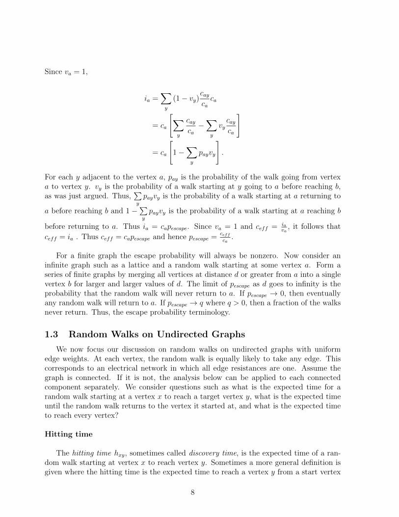
Proof: Now t (n) = 1 since the walk stops when it reaches vertex n. Half of the time whenthe walk is at vertex n − 1 it goes to vertex n. Thus t (n− 1) = 2. For 3 ≤ i ≤ n− 1,t (i) = 1

2[t (i− 1) + t (i+ 1)] and t (1) and t (2) satisfy t (1) = 1

2t (2) + 1 and t (2) =

t (1) + 12t (3). Solving for t(i+ 1) for 3 ≤ i ≤ n− 1 yields

t(i+ 1) = 2t(i)− t(i− 1)

which has solution t(i) = 2(n− i) for 3 ≤ i ≤ n− 1. Then solving for t(2) and t(1) yieldst (2) = 2 (n− 2) and t (1) = n− 1. Thus, the total time spent at vertices is

n− 1 + 2 (1 + 2 + · · ·+ n− 2) + 1 = n− 1 + (n− 1)(n− 2) + 1 = (n− 1)2 + 1

which is one more than h1n and thus is correct.

Next we show that adding edges to a graph might either increase or decrease thehitting time hxy. Consider the graph consisting of a single path of n vertices. Add edgesto this graph to get the graph in Figure 1.1 consisting of a clique of size n/2 connectedto a path of n/2 vertices. Then add still more edges to get a clique of size n. Let x bethe vertex at the midpoint of the original path and let y be the other endpoint of thepath consisting of n/2 vertices as shown in Figure 1.1. In the first graph consisting of asingle path of length n, hxy = Θ (n2). In the second graph consisting of a clique of sizen/2 along with a path of length n/2, hxy = Θ (n3). To see this latter statement, notethat starting at x, the walk will go down the chain towards y and return to x n times onaverage before reaching y for the first time. Each time the walk in the chain returns tox, with probability (n − 1)/n it enters the clique and thus on average enters the cliqueΘ(n) times before starting down the chain again. Each time it enters the clique, it spendsΘ(n) time in the clique before returning to x. Thus, each time the path returns to x fromthe chain it spends Θ(n2) time in the clique before starting down the chain towards y fora total expected time that is Θ(n3) before reaching y. In the third graph, which is theclique of size n, hxy = Θ (n). Thus, adding edges first increased hxy from n2 to n3 andthen decreased it to n.

Hitting time is not symmetric even in the case of undirected graphs. In the graph ofFigure 1.1, the expected time, hxy, of a random walk from x to y, where x is the vertex ofattachment and y is the other end vertex of the chain, is Θ(n3). However, hyx is Θ(n2).

Next we ask what is the maximum that the hitting time could be. We first show thatif vertices x and y are connected by an edge, then the expected time, hxy, of a randomwalk from x to y plus the expected time, hyx, from y to x is at most twice the number ofedges.

Lemma 1.4 If vertices x and y are connected by an edge, then hxy + hyx ≤ 2m where mis the number of edges in the graph.

10

xy

n/2

︸ ︷︷ ︸

clique ofsize n/2

Figure 1.1: Illustration that adding edges to a graph can either increase or decrease hittingtime.

Proof: In a random walk on an undirected graph starting in the steady state, the prob-ability of traversing any edge in either direction is 1/(2m). This is because for any edge(u, v), the probability of being at u (in the steady state) is du/(2m) and the probabilityof selecting the edge (u, v) is 1/du. Hence, the probability of traversing the edge (u, v)is 1/(2m) implying that the expected time between traversals of the edge (x, y) from xto y is 2m. Thus, if we traverse edge (x, y), the expected time to traverse a path fromy back to x and then traverse the edge (x, y) again is 2m. But since a random walk isa memory less process, we can drop the condition that we started by traversing the edge(x, y). Hence the expected time from y to x and back to y is at most 2m. Note thatthe path went from y to x and then may have returned to x several times before goingthrough the edge (x, y). Thus, the less than or equal sign in the statement of the lemmasince the path have gone from y to x to y without going through the edge (x, y).

Notice that the proof relied on the fact that there was an edge from x to y and thusthe theorem is not necessarily true for arbitrary x and y. When x and y are not con-nected by an edge consider a path from x to y. The path is of length at most n. Considerthe time it takes to reach each vertex on the path in the order they appear. Since thevertices on the path are connected by edges, the expected time to reach the next vertexon the path is at most twice the number of edges in the graph by the above theorem.Thus, the total expected time is Θ (n3). This result is asymptotically tight since the boundis met by the graph of Figure 1.1 consisting of a clique of size n/2 and a path of length n/2.

Commute time

The commute time, commute(x, y), is the expected time of a random walk starting atx reaching y and then returning to x. Think of going from home to office and returninghome.

Theorem 1.5 Given an undirected graph, consider the electrical network where each edgeof the graph is replaced by a one ohm resistor. Given vertices x and y, the commute time,

11

commute(x, y), equals 2mrxy where rxy is the effective resistance from x to y and m is thenumber of edges in the graph.

Proof: Insert at each vertex i a current equal to the degree di of vertex i. The totalcurrent inserted is 2m where m is the number of edges. Extract from a specific vertex jall of this 2m current. Let vij be the voltage difference from i to j. The current into idivides into the di resistors at node i. The current in each resistor is proportional to thevoltage across it. Let k be a vertex adjacent to i. Then the current through the resistorbetween i and k is vij − vkj, the voltage drop across the resister. The sum of the currentsout of i through the resisters must equal di, the current injected into i.

di =∑k adjto i

(vij − vkj)

Noting that vij does not depend on k, write

di = divij −∑k adjto i

vkj.

Solving for vij

vij = 1 +∑k adjto i

1divkj =

∑k adjto i

1di

(1 + vkj). (1.1)

Now the expected time from i to j is the average time over all paths from i to kadjacent to i and then on from k to j. This is given by

hij =∑k adjto i

1di

(1 + hkj). (1.2)

Subtracting (1.2) from (1.1), gives vij−hij =∑k adjto i

1di

(vkj − hkj). Thus, the function vij−hij

is harmonic. Designate vertex j as the only exterior vertex. The value of vij − hij at j,namely vjj − hjj, is zero, since both vjj and hjj are zero. So the function vij − hij mustbe zero everywhere. Thus, the voltage vij equals the expected time hij from i to j.

To complete the proof, note that hij = vij is the voltage from i to j when currentsare inserted at all nodes in the graph and extracted at node j. If the current is extractedfrom i instead of j, then the voltages change and vji = hji in the new setup. Finally,reverse all currents in this latter step. The voltages change again and for the new voltages−vji = hji. Since −vji = vij, we get hji = vij.

12

Thus, when a current is inserted at each node equal to the degree of the node and thecurrent is extracted from j, the voltage vij in this set up equals hij. When we extract thecurrent from i instead of j and then reverse all currents, the voltage vij in this new setup equals hji. Now, superpose both situations (i.e., add all the currents and voltages).By linearity, for the resulting vij, vij = hij + hji. All currents cancel except the 2m ampsinjected at i and withdrawn at j. Thus, 2mrij = vij = hij + hji = commute(i, j). Thus,commute(i, j) = 2mrij.

Note that Lemma 1.4 also follows from Theorem 1.5 since the effective resistance ruvis less than or equal to 1 when u and v are connected by an edge.

Corollary 1.6 For any n vertex graph and for any vertices x and y, the commute time,commute(x, y), is less than or equal to n3.

Proof: By Theorem 1.5 the commute time is given by the formula commute(x, y) =2mrxy where m is the number of edges. In an n vertex graph there exists a path fromx to y of length at most n. This implies rxy ≤ n since the resistance can not be greaterthan that of any path from x to y. Since the number of edges is at most

(n2

)commute(x, y) = 2mrxy ≤ 2

(n

2

)n ∼= n3.

Again adding edges to a graph may increase or decrease the commute time. To see this,consider the graph consisting of a chain of n vertices, the graph of Figure 1.1, and theclique on n vertices.

Cover times

The cover time cover(x,G) is the expected time of a random walk starting at vertex xin the graph G to reach each vertex at least once. We write cover(x) when G is understood.The cover time of an undirected graph G, denoted cover(G), is

cover(G) = maxx

cover(x,G).

For cover time of an undirected graph, increasing the number of edges in the graphmay increase or decrease the cover time depending on the situation. Again consider threegraphs, a chain of length n which has cover time Θ(n2), the graph in Figure 1.1 which hascover time Θ(n3), and the complete graph on n vertices which has cover time Θ(n log n).Adding edges to the chain of length n to create the graph in Figure 1.1 increases thecover time from n2 to n3 and then adding even more edges to obtain the complete graphreduces the cover time to n log n.

13

Note: The cover time of a clique is n log n since that is the time to select every in-teger out of n integers with high probability, drawing integers at random. This is calledthe coupon collector problem. The cover time for a straight line is Θ(n2) since it is thesame as the hitting time. For the graph in Figure 1.1, the cover time is Θ(n3) since onetakes the maximum over all start states and cover(x,G) = Θ (n3).

Theorem 1.7 Let G be a connected graph with n vertices and m edges. The time for arandom walk to cover all vertices of the graph G is bounded above by 2m(n− 1).

Proof: Consider a depth first search (dfs) of the graph G starting from vertex z andlet T be the resulting dfs spanning tree of G. The dfs covers every vertex. Consider theexpected time to cover every vertex in the order visited by the depth first search. Clearlythis bounds the cover time of G starting from vertex z.

cover (z,G) ≤∑

(x,y)∈T

hxy.

If (x, y) is an edge in T , then x and y are adjacent and thus Lemma 1.4 implies hxy ≤ 2m.Since there are n − 1 edges in the dfs tree and each edge is traversed twice, oncein each direction, cover(z) ≤ 2m(n − 1). Since this holds for all starting vertices z,cover(G) ≤ 2m(n− 1)

The theorem gives the correct answer of n3 for the n/2 clique with the n/2 tail. Itgives an upper bound of n3 for the n-clique where the actual cover time is n log n.

Let rxy be the effective resistance from x to y. Define the resistance r(G) of a graphG by r(G) = max

x,y(rxy).

Theorem 1.8 Let G be an undirected graph with m edges. Then the cover time for G isbounded by the following inequality

mr(G) ≤ cover(G) ≤ 2e3mr(G) lnn+ n

where e=2.71 is Euler’s constant and r(G) is the resistance of G.

Proof: By definition r(G) = maxx,y

(rxy). Let u and v be the vertices of G for which

rxy is maximum. Then r(G) = ruv. By Theorem 1.5, commute(u, v) = 2mruv. Hencemruv = 1

2commute(u, v). Clearly the commute time from u to v and back to u is less

than twice the max(huv, hvu) and max(huv, hvu) is clearly less than the cover time of G.Putting these facts together

mr(G) = mruv = 12commute(u, v) ≤ max(huv, hvu) ≤ cover(G).

For the second inequality in the theorem, by Theorem 1.5, for any x and y commute(x, y)equals 2mrxy implying hxy ≤ 2mr(G). By the Markov inequality, since the expected value

14

of hxy is less than 2mr(G), the probability that y is not reached from x in 2mr(G)e3 stepsis at most 1

e3. Thus, the probability that a vertex y has not been reached in 2e3mr(G) log n

steps is at most 1e3

lnn= 1

n3 because a random walk of length 2e3mr(G) log n is a sequenceof log n independent random walks, each of length 2e3mr(G). Suppose after a walk of2e3mr(G) log n steps, vertices v1, v2, . . . , vl where not reached. Walk until v1 is reached,then v2, etc. By Corollary 1.6 the expected time for each of these is n3, but since eachhappens only with probability 1/n3, we effectively take O(1) time per vi, for a total timeof at most n.

Return time

The return time is the expected time of a walk starting at x returning to x. We explorethis quantity later.

1.4 Random Walks in Euclidean Space

Many physical processes such as Brownian motion are modeled by random walks.Random walks in Euclidean d-space consisting of fixed length steps parallel to the coor-dinate axes are really random walks on a d-dimensional lattice and are a special case ofrandom walks on graphs. In a random walk on a graph, at each time unit an edge fromthe current vertex is selected at random and the walk proceeds to the adjacent vertex.We begin by studying random walks on lattices.

Random walks on lattices

We now apply the analogy between random walks and current to lattices. Considera random walk on a finite segment −n, . . . ,−1, 0, 1, 2, . . . , n of a one dimensional latticestarting from the origin. Is the walk certain to return to the origin or is there some prob-ability that it will escape, i.e., reach the boundary before returning? The probability ofreaching the boundary before returning to the origin is called the escape probability. Weshall be interested in this quantity as n goes to infinity.

Convert the lattice to an electrical network by replacing each edge with a one ohmresister. Then the probability of a walk starting at the origin reaching n or –n beforereturning to the origin is the escape probability given by

pescape =ceffca

where ceff is the effective conductance between the origin and the boundary points and cais the sum of the conductance’s at the origin. In a d-dimensional lattice, ca = 2d assumingthat the resistors have value one. For the d-dimensional lattice

pescape =1

2d reff

15

(a)

4 12 20

0 1 2 3

Number of resistorsin parallel

(b)

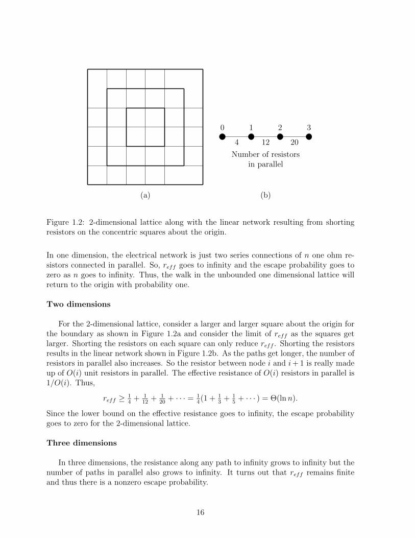
Figure 1.2: 2-dimensional lattice along with the linear network resulting from shortingresistors on the concentric squares about the origin.

In one dimension, the electrical network is just two series connections of n one ohm re-sistors connected in parallel. So, reff goes to infinity and the escape probability goes tozero as n goes to infinity. Thus, the walk in the unbounded one dimensional lattice willreturn to the origin with probability one.

Two dimensions

For the 2-dimensional lattice, consider a larger and larger square about the origin forthe boundary as shown in Figure 1.2a and consider the limit of reff as the squares getlarger. Shorting the resistors on each square can only reduce reff . Shorting the resistorsresults in the linear network shown in Figure 1.2b. As the paths get longer, the number ofresistors in parallel also increases. So the resistor between node i and i+ 1 is really madeup of O(i) unit resistors in parallel. The effective resistance of O(i) resistors in parallel is1/O(i). Thus,

reff ≥ 14

+ 112

+ 120

+ · · · = 14(1 + 1

3+ 1

5+ · · · ) = Θ(lnn).

Since the lower bound on the effective resistance goes to infinity, the escape probabilitygoes to zero for the 2-dimensional lattice.

Three dimensions

In three dimensions, the resistance along any path to infinity grows to infinity but thenumber of paths in parallel also grows to infinity. It turns out that reff remains finiteand thus there is a nonzero escape probability.

16

Figure 1.3: Paths in a 2-dimensional lattice obtained from the 3-dimensional constructionapplied in 2-dimensions.

The construction used in three dimensions is easier to explain first in two dimensions.Draw dotted diagonal lines at x+ y = 2n−1. Consider two paths that start at the origin.One goes up and the other goes to the right. Each time a path encounters a dotteddiagonal line, split the path into two, one which goes right and the other up. Wheretwo paths cross, split the vertex into two, keeping the paths separate. By a symmetryargument, splitting the vertex does not change the resistance of the network. Removeall resistors except those on these paths. The resistance of the original network is lessthan that of the tree produced by this process since removing a resistor is equivalent toincreasing its resistance to infinity.

The distances between splits increase and are 1, 2, 4, etc. At each split the number ofpaths in parallel doubles. Thus, the resistance to infinity in this two dimensional exampleis

1

2+

1

42 +

1

84 + · · · = 1

2+

1

2+

1

2+ · · · =∞.

In the analogous three dimensional construction, paths go up, to the right, and out ofthe plane of the paper. The paths split three ways at planes given by x+ y + z = 2n − 1.

17

Each time the paths split the number of parallel segments triple. Segments of the pathsbetween splits are of length 1, 2, 4, etc. and the resistance of the segments are equal tothe lengths. The resistance out to infinity for the tree is

13

+ 192 + 1

274 + · · · = 1

3

(1 + 2

3+ 4

9+ · · ·

)= 1

31

1− 23

= 1

The resistance of the three dimensional lattice is less. Thus, in three dimensions theescape probability is nonzero. The upper bound on reff gives the lower bound

pescape = 12d

1reff≥ 1

6.

A lower bound on reff gives an upper bound on pescape. To get the upper bound on pescape,short all resistors on surfaces of boxes at distances 1, 2, 3,, etc. Then

reff ≥ 16

[1 + 1

9+ 1

25+ · · ·

]≥ 1.23

6≥ 0.2

This givespescape = 1

2d1

reff≥ 5

6.

1.5 Random Walks on Directed Graphs

A major application of random walks on directed graphs comes from trying to establishthe importance of pages on the World Wide Web. One way to do this would be to takea random walk on the web and rank pages according to their stationary probability.However, several situations occur in random walks on directed graphs that did not arisewith undirected graphs. One difficulty occurs if there is a node with no out edges. In thiscase, the directed graph is not strongly connected and so Markov chain is not stronglyconnected either even though the underlying undirected graph may be connected. Whenthe walk encounters this node the walk disappears. Another difficulty is that a node ora strongly connected component with no in edges is never reached. One way to resolvethese difficulties is to introduce a random restart condition. At each step, with someprobability r, jump to a node selected uniformly at random and with probability 1 − rselect an edge at random and follow it. If a node has no out edges, the value of r for thatnode is set to one. This has the effect of converting the graph to a strongly connectedgraph so that the stationary probabilities exist.

1.6 Finite Markov Processes

A Markov process is a random process in which the probability distribution for thefuture behavior depends only on the current state, not on how the process arrived atthe current state. Markov processes are equivalent mathematically to random walks ondirected graphs but the literature on the two topics developed separately with differentterminology. Since much of the terminology of Markov processes appears in the literatureon random walks, we introduce the terminology here to acquaint the reader with it.

18

A B C(a)

A B C(b)

Figure 1.4: (a) A directed graph with nodes with no out out edges and a strongly con-nected component A with no in edges.(b) A directed graph with three strongly connected components.

In a Markov process, nodes of the underlying graph are referred to as states. A stateis persistent if it has the property that should the state ever be reached, the randomprocess will return to it with probability one. This means that the state is in a stronglyconnected component with no out edges. Consider the directed graph in Figure 1.4b withthree strongly connected components A, B, and C. Starting from any node in A thereis a nonzero probability of eventually reaching any node in A. However, the probabilityof returning to a node in A is less than one and thus nodes in A and similarly nodes inB are not persistent. From any node in C, the walk will return with probability one tothat node eventually since there is no way of leaving component C. Thus, nodes in C arepersistent.

A state is periodic if it is contained only in cycles in which the greatest common divisor(gcd) of the cycle lengths is greater than one. A Markov process is irreducible if it consistsof a single strongly connected component. An ergodic state is one that is aperiodic andpersistent. A Markov process is ergodic if all states are ergodic. In graph theory thiscorresponds to a single strongly connected component that is aperiodic.

Page rank and hitting time

The page rank of a node in a directed graph is the stationary probability of the node.We assume some restart value, say r = 0.15, is used. The restart ensures that the graphis strongly connected. The page rank of a page is the fractional frequency with which the

19

ijpji

120.85πi

120.85πi

0.15πi

πi = πjpji + 0.852πi

πi = 1.74(πjpji)

Figure 1.5: Impact on page rank of adding a self loop

page will be visited over a long period of time. If the page rank is p, then the expectedtime between visits or return time is 1/p. Notice that one can increase the pagerank of apage by reducing the return time and this can be done by creating short cycles.

Consider a node i with a single edge in from node j and a single edge out. Thestationary probability π satisfies πP = π, and thus

πi = πjpji.

Adding a self-loop at i, results in a new equation

= pii = πjpji +1

2πi

orπi = 2 πjpji.

Of course, πj would have changed too, but ignoring this for now, pagerank is doubled bythe addition of a self-loop. Adding k self loops, results in the equation

πi = πjpji +k

k + 1πi,

and again ignoring the change in πj, we now have πi = (k + 1)πjpji. What preventsone from increasing the page rank of a page arbitrarily? The answer is the restart. Weneglected the 0.15 probability that is taken off for the random restart. With the restarttaken into account, the equation for πi when there is no self-loop is

πi = 0.85πjpji

whereas, with k self-loops, the equation is

πi = 0.85πjpji + 0.85k

k + 1πi.

Adding a single loop only increases pagerank by a factor of 1.74 and adding k loops in-creases it by at most a factor of 6.67 for arbitrarily large k.

20

Hitting time

Related to page rank is a quantity called hitting time. Hitting time is closely relatedto return time and thus to the reciprocal of page rank. One way to return to a nodev is by a path in the graph from v back to v. Another way is to start on a path thatencounters a restart, followed by a path from the random restart node to v. The timeto reach v after a restart is the hitting time. Thus, return time is clearly less than theexpected time until a restart plus hitting time. The fastest one could return would be ifthere were only paths of length two since self loops are ignored in calculating page rank. Ifr is the restart value, then the loop would be traversed with at most probability (1− r)2.With probability r + (1− r) r = (2− r) r one restarts and then hits v. Thus, the returntime is at least (1− r)2 + (2− r) r × (hitting time). Combining these two bounds yields

(1− r)2 + (2− r) rE (hitting time) ≤ E (return time) ≤ E (hitting time)

The relationship between return time and hitting time can be used to see if a node hasunusually high probability of short loops. However, there is no efficient way to computehitting time for all nodes as there is for return time. For a single node v, one can computehitting time by removing the edges out of the node v for which one is computing hittingtime and then run the page rank algorithm for the new graph. The hitting time for vis the reciprocal of the page rank in the graph with the edges out of v removed. Sincecomputing hitting time for each node requires removal of a different set of edges, thealgorithm only gives the hitting time for one node at a time. Since one is probably onlyinterested in the hitting time of nodes with low hitting time, an alternative would be touse a random walk to estimate the hitting time of low hitting time nodes.

Spam

Suppose one has a web page and would like to increase its page rank by creating someother web pages with pointers to the original page. The abstract problem is the following.We are given a directed graph G and a node v whose page rank we want to increase. Wemay add new nodes to the graph and add edges from v or from the new nodes to anynodes we want. We cannot add edges out of other nodes. We can also delete edges from v.

The page rank of v is the stationary probability for node v with random restarts. Ifwe delete all existing edges out of v, create a new node u and edges (v, u) and (u, v),then the page rank will be increased since any time the random walk reaches v it willbe captured in the loop v → u → v. A search engine can counter this strategy by morefrequent random restarts.

A second method to increase page rank would be to create a star consisting of thenode v at its center along with a large set of new nodes each with a directed edge to v.These new nodes will sometimes be chosen as the target of the random restart and hence

21

the nodes increase the probability of the random walk reaching v. This second method iscountered by reducing the frequency of random restarts.

Notice that the first technique of capturing the random walk increases page rank butdoes not effect hitting time. One can negate the impact of someone capturing the randomwalk on page rank by increasing the frequency of random restarts. The second techniqueof creating a star increases page rank due to random restarts and decreases hitting time.One can check if the page rank is high and hitting time is low in which case the pagerank is likely to have been artificially inflated by the page capturing the walk with shortcycles.

Personalized page rank

In computing page rank, one uses a restart probability, typically 0.15, in which at eachstep, instead of taking a step in the graph, the walk goes to a node selected uniformly atrandom. In personalized page rank, instead of selecting a node uniformly at random, oneselects a node according to a personalized probability distribution. Often the distributionhas probability one for a single node and whenever the walk restarts it restarts at thatnode.

Algorithm for computing personalized page rank

First, consider the normal page rank. Let α be the restart probability with whichthe random walk jumps to an arbitrary node. With probability 1 − α the random walkselects a node uniformly at random from the set of adjacent nodes. Let p be a row vectordenoting the page rank and let G be the adjacency matrix with rows normalized to sumto one. Then

p = αn

(1, 1, . . . , 1) + (1− α) pG

p[I − (1− α)G] =α

n(1, 1, . . . , 1)

orp = α

n(1, 1, . . . , 1) [I − (1− α)G]−1.

Thus, in principle, p can be found by computing the inverse of [I − (1 − α)G]−1. Butthis is far from practical since for the whole web one would be dealing with matrices withbillions of rows and columns. A more practical procedure is to run the random walk andobserve using the basics of the power method in Chapter ?? that the process convergesto the solution p.

For the personalized page rank, instead of restarting at an arbitrary vertex, the walkrestarts at a designated vertex. More generally, it may restart in some specified neighbor-hood. Suppose the restart selects a vertex using the probability distribution s. Then, in

22

the above calculation replace the vector 1n

(1, 1, . . . , 1) by the vector s. Again, the compu-tation could be done by a random walk. But, we wish to do the random walk calculationfor personalized pagerank quickly since it is to be performed repeatedly. With more carethis can be done, though we do not describe it here.

1.7 Markov Chain Monte Carlo

The Markov Chain Monte Carlo method is a technique for sampling a multivariateprobability distribution p(x), where x = (x1, x2, . . . , xd) is the set of variables. Given theprobability distribution p (x), one might wish to calculate the marginal distribution

p (x1) =∑

x2,...,xd

p (x1, . . . , xd)

or the expectation of some functionf (x)

E (f) =∑

x1,...,xd

f (x1, . . . , xd) p (x1, . . . , xd).

The difficulty is that both computations require a summation over an exponential numberof values. If each xi can take on a value from the set 1, 2, . . . , n of values, then thereare nd possible values for x. One could compute an approximate answer by generatinga sample set of values for x = (x1, . . . , xd) according to the distribution p (x1, . . . , xd).This is done by designing a Markov chain whose stationary probabilities are exactlyp(x1, x2, . . . , xd) and running the chain for a sufficiently large number of steps and aver-aging f over the states seen in the run. The number of steps must be large enough thatwe are close to the limit which is the stationary distribution. In the rest of this section,we will show that under some mild conditions, the number of steps needed grows onlypolynomially, though the total number of states grows exponentially with d.

For ease of explanation, assume that the variables take on values from some finiteset. Create a directed graph with one node corresponding to each possible value of x. Arandom walk on the the graph is designed so that the stationary probability of the walk isp(x). The walk is designed by specifying the probability of the transition from one nodeto another in such a way as to achieve the desired stationary distribution. Two commontechniques for designing the walks are the Metropolis-Hasting algorithm and Gibbs sam-pling. We will see that the sequence of nodes after a sufficient number of steps of the walkprovides a good sample of the distribution. The number of steps the walk needs to takedepends on its convergence rate to its stationary distribution. We will show that this rateis related to a natural quantity called the minimum escape probability (MEP).

We used x ∈ Rd to emphasize that our distributions are multi-variate. From a Markovchain perspective, each value x can take on is a state, i.e., a node of the graph on which

23

the random walk takes place. Henceforth, we will use the subscripts i, j, k, . . . to denotestates and will use pi instead of p(x1, x2, . . . , xd) to denote the probability of the statecorresponding to a given set of values for the variables. Recall that in the Markov chainterminology, nodes of the graph are called states.

Recall the notation that p(t) is the row vector of probabilities of the random walkbeing at each state (node of the graph) at time t. So, p(t) has as many components as

there are states and its ith component, p(t)i , is the probability of being in state i at time

t. Recall the long-term (t-step) average is

a(t) =1

t

[p(0) + p(1) + · · ·+ p(t−1)

]. (1.3)

The expected value of the function f under the probability distribution p is E(f) =∑i fipi. Our estimate of this quantity will be the average value of f at the states seen in

a t step run. Call this estimate a. Clearly, the expected value of a is

E(a) =∑i

fia(t)i .

The expectation here is with respect to the “coin tosses” of the algorithm, not with respectto the underlying distribution p. Letting fmax denote the maximum absolute value of f .It is easy to see that∣∣∣∣∣E(a)−

∑i

fipi

∣∣∣∣∣ ≤ fmax

∑i

|pi − a(t)i | = fmax|p− a(t)|1 (1.4)

where the quantity |p − a(t)|1 is the l1 distance between the probability distributions pand a(t) and is often called the “total variation distance” between the distributions. Wewill build tools to upper bound |p− a(t)|1. Since p is the steady state distribution, the tfor which |p−a(t)|1 becomes small is determined by the rate of convergence of the Markovchain to its steady state.

The following proposition is often useful.

Proposition 1.9 For two probability distributions p and q, |p− q|1 = 2∑

i(pi − qi)+ =2∑

i(qi − pi)+.

The proof is left as an exercise (Exercise 1.34).

1.7.1 Time Reversibility

Definition: A Markov chain is said to be time-reversible if for the steady state proba-bilities π, πipij = πjpji for all i and j.

24

The phrase “time-reversible” comes from the following fact. For a time-reversible Markovchain started in the steady state, the probability of a path (sequence of states) is the sameas its reversal. That is

πi1 pi1,i2pi2,i3 · · · pik−1,ik = πik pik,ik−1pik−1,ik−2

· · · pi2,i1 .

Given only the sequence of states seen, one cannot tell if time runs forward or backward,both having the same probability. More important is the fact that time reversibilitysimplifies the underlying mathematics as illustrated in the following lemma. The lemmastates that if a probability distribution q has the property that the probability of traversingeach edge is the same in both directions, then the probability distribution must be thesteady state distribution of the Markov chain. The lemma is used frequently.

Lemma 1.10 In a strongly connected Markov chain with transition probabilities pij, if avector q with non-negative components satisfies

qipij = qjpji

for all i and j, then qi/∑k

qk is the stationary probability of node i.

Proof: Since the chain is strongly connected, there is a unique stationary probabilityvector π satisfying the equations πP = π and

∑i πi = 1. Now q/

∑k qk satisfies these

equations since∑

i qi/∑

k qk = 1 and for each fixed j,∑

i qipij =∑

i qjpji = qj∑

i pji = qj.Thus q must be the steady state distribution.

1.7.2 Metropolis-Hasting Algorithm

Metropolis-Hasting algorithm is a general method to design a Markov chain whosestationary distribution is a given target distribution p. Start with a connected undirectedgraphG on the set of states. For example, if the states are the lattice points (x1, x2, . . . , xd)in Rd with xi ∈ 0, 1, 2, , . . . , n, then G is the lattice graph with 2d coordinate edgesat each interior vertex. In general, let r be the maximum degree of any node of G. Thetransitions of the Markov chain are defined as follows. At state i select neighbor j withprobability 1

r. Since the degree of i may be less than r, with some probability no edge

is selected and the walk remains at i. If a neighbor j is selected and pj ≥ pi, go to j. Ifpj < pi, go to j with probability pj/pi and stay at i with probability 1− pj

pi. Intuitively, this

favors “heavier” states with higher p values. For i and j adjacent in G, pij = 1r

min(

1,pjpi

)and pii = 1−

∑j 6=i

pij. Then

pipij =pir

min

(1,pjpi

)=

1

rmin(pi, pj) =

pjd

min

(1,pipj

)= pjpji.

By Lemma 1.10, the stationary probabilities are p(x) as desired.

25

d

a

c

b

18

12

18

14

p(a) = 12

p(b) = 14

p(c) = 18

p(d) = 18

a→ b 13

14

21

= 16

c→ a 13

a→ c 13

18

21

= 112

c→ b 13

a→ d 13

18

21

= 112

c→ d 13

a→ a 23

c→ c 1− 13− 1

3− 1

3= 0

b→ a 13

d→ a 13

b→ c 13

18

41

= 16

d→ c 13

b→ b 1− 13− 1

6= 1

2d→ d 1− 1

3− 1

3= 1

3

p(a) = p(a)p(a→ a) + p(b)p(b→ a) + p(c)p(c→ a) + P (d)p(d→ a)= 1

223

+ 14

13

+ 18

13

+ 18

13

= 12

p(b) = p(a)p(a→ b) + p(b)p(b→ b) + p(c)p(c→ b)= 1

216

+ 14

12

+ 18

13

= 14

p(c) = p(a)p(a→ c) + p(b)p(b→ c) + p(c)p(c→ c) + P (d)p(d→ c)= 1

2112

+ 14

16

+ 18

0 + 18

13

= 18

p(d) = p(a)p(a→ d) + p(c)p(c→ d) + P (d)p(d→ d)= 1

2112

+ 18

13

+ 18

13

= 18

Figure 1.6: Using the Metropolis-Hasting algorithm to set probabilities for a random walkso that the stationary probability will be a desired probability.

Example: Consider the graph in Figure 1.6. Using the Metropolis-Hasting algorithm,assign transition probabilities so that the stationary probability of a random walk isp(a) = 1

2, p(b) = 1

4, p(c) = 1

8, and p(d) = 1

8. The maximum degree of any vertex is three

so at a the probability of taking the edge (a, b) is 13

14

21

or 16. The probability of taking the

edge (a, c) is 13

18

21

or 112

and of taking the edge (a, d) is 13

18

21

or 112

. Thus the probabilityof staying at a is 2

3. The probability of taking the edge from b to a is 1

3. The probability

of taking the edge from c to a is 13

and the probability of taking the edge from d to ais 1

3. Thus the stationary probability of a is 1

413

+ 18

13

+ 18

13

+ 12

23

= 12, which is what is

desired.

1.7.3 Gibbs Sampling

Gibbs sampling is another Markov Chain Monte Carlo method to sample from amultivariate probability distribution. Let p (x) be the target distribution where x =(x1, . . . , xd). Gibbs sampling consists of a random walk on a graph whose vertices corre-spond to the values of x = (x1, . . . , xd) and in which there is an edge from x to y if x andy differ in only one coordinate.

26

To generate samples of x = (x1, . . . , xd) with a target distribution p (x), the Gibbssampling algorithm repeats the following steps. One of the variables xi is chosen to beupdated. Its new value is chosen based on the marginal probability of xi with the othervariables fixed. There are two commonly used schemes to determine which xi to update.One scheme is to choose xi randomly, the other is to choose xi by sequentially scanningfrom x1 to xd.

Suppose that x and y are two states that differ in only one coordinate xi. Then, inthe scheme where a coordinate is randomly chosen to modify, the probability pxy of goingfrom x to y is

pxy =1

dp(yi|x1, x2, . . . , xi−1, xi+1, . . . , xd).

The normalizing constant is 1/d since for a given value i the probability distribution ofp(yi|x1, x2, . . . , xi−1, xi+1, . . . , xd) sums to one, and thus summing i over the d-dimensionsresults in a value of d. Similarly,

pyx =1

dp(xi|x1, x2, . . . , xi−1, xi+1, . . . , xd).

Here use was made of the fact that for j 6= i, xj = yj.

It is simple to see that this chain is time reversible with stationary probability pro-portional to p (x). Rewrite pxy as

pxy =1

d

p(yi|x1, x2, . . . , xi−1, xi+1, . . . , xd)p(x1, x2, . . . , xi−1, xi+1, . . . , xd)

p(x1, x2, . . . , xi−1, xi+1, . . . , xd)

=1

d

p(x1, x2, . . . , xi−1, yi, xi+1, . . . , xd)

p(x1, x2, . . . , xi−1, xi+1, . . . , xd)

=1

d

p(y)

p(x1, x2, . . . , xi−1, xi+1, . . . , xd)

again using xj = yj for j 6= i. Similarly write

pyx =1

d

p(x)

p(x1, x2, . . . , xi−1, xi+1, . . . , xd)

from which it follows that p(x)pxy = p(y)pyx. By Lemma 1.10 the stationary probabilityof the random walk is p(x).

1.8 Convergence to Steady State

The Metropolis-Hasting algorithm and Gibbs sampling both involve a random walk.Initial states of the walk are highly dependent on the start state of the walk. An impor-tant question is how fast does the walk start to reflect the stationary probability of the

27

Figure 1.7: A constriction.

Markov process. If the convergence time was proportional to the number of states thealgorithms would not be very useful, since as we remarked, the number of states can beexponentially large.

There are clear examples of connected chains that take a long time to converge. Achain with a constriction (see Figure 1.7) takes a long time to converge since the walk isunlikely to reach the narrow passage between the two halves, which are both reasonablybig. The interesting thing is that a converse is also true. If there is no constriction, thenthe chain converges fast. We show this shortly.

A function is unimodal if it has a single maximum, i.e., it increases and then decreases..A unimodal function like the normal density has no constriction blocking a random walkfrom getting out of a large set, whereas a bimodal function can have a constriction.Interestingly, many common multivariate distributions as well as univariate probabilitydistributions like the normal and exponential are unimodal and sampling according tothese distributions can be done using the methods here.

A natural problem is estimating the probability of a convex region in d-space accordingto a normal distribution. Let R be the region defined by the inequality x1+x2+· · ·+xd/2 ≤x(d/2)+1 + · · ·+xd. Pick a sample according to the normal distribution and accept the sam-ple if it satisfies the inequality. If not, reject the sample and retry until one gets a numberof samples satisfying the inequality. Then the probability of the region is approximatedby the fraction of the samples that satisfied the inequality. However, suppose R was theregion x1 + x2 + · · · + xd−1 ≤ xd. The probability of this region is exponentially smallin d and so rejection sampling runs into the problem that we need to pick exponentiallymany samples before we expect to accept even one sample. This second situation is typ-ical. Imagine computing the probability of failure of a system. The object of design is to

28

Figure 1.8: Area enclosed by curve.

make the system reliable, so the failure probability is likely to be very low and rejectionsampling will take a long time to estimate the failure probability.

A similar problem is one of computing areas and volumes. First consider the problemof computing the area enclosed by the curve in Figure 1.8. One method would be to find a“nicer” enclosing shape. The picture on the right shows a convex polygon whose area wecan compute in closed form by adding up the areas of the triangles. Throw darts at thelarger shape, i.e., pick samples uniformly at random from the larger shape, and estimatethe ratio of areas by the proportion of samples that land in the area enclosed by the curve.

Such methods fail in higher dimensions. For example, to compute the volume of ad-dimensional sphere by enclosing the sphere in a cube where the ratio of volume of thesphere to the cube is exponentially small, requires throwing exponentially many dartsbefore getting any nonzero answer.

A different way to solve the problem of drawing a uniform random sample from ad-dimensional region is to put a grid on the region and do a random walk on the gridpoints. At each time, pick one of the 2d coordinate neighbors of the current grid point,each with probability 1/(2d), then go to the neighbor if it is still in the set; otherwise, stayput and repeat. This can be shown to lead to a polynomial time algorithm for drawing auniform random sample from a bounded convex d-dimensional region. It turns out thatthis can be used to estimate volumes of such a region by immersing the region in a magni-fied copy of itself intersected with a nice object like a cube. We do not give the details here.

In general, there could be constrictions that prevent rapid convergence to the station-ary probability. However, if the set is convex in any number of dimensions, then there are

29

S S

Figure 1.9: Each grid point in the ellipse is a state. The set of states in the ellipseis divided into two sets, S and S, by the curve. The transitions from S to S, whichcontribute to Φ(S), are marked with arrows.

no constrictions and there is rapid convergence although the proof of this is beyond thescope of this book.

Suppose q is any probability distribution on the states. Execute one step of the Markovchain starting with distribution q. Then the amount of probability that “flows” from i toj is qipji. If S and T are two possibly intersecting subsets of states, the total flow from Sto T is

∑i∈S,j∈T

qipij. We use the notation

flow(i, j) = qipij

andflow(S, T )) =

∑i∈S,j∈T

qipij.

We define below a combinatorial measure of constriction for a Markov chain, called theminimum escape probability, and relate this quantity to the rate of convergence to thestationarity probability.1

1In the Markov Chain literature, the word “conductance” is often used for minimum escape probability.Here, we have reserved the word conductance for the natural electrical quantity which is the reciprocalof resistance.

30

Definition: For a subset S of states of a Markov chain with stationary probabilities π,define Φ(S), the escape probability of S, by

Φ(S) =flow(S, S)

π(S).

The escape probability of S is the probability of taking a step from S to outside Sconditioned on starting in S where the stationary probability at state i in S is proportionalto its stationary probability, i.e., πi/π(S). The minimum escape probability MEP of theMarkov chain, denoted Φ, is defined by

Φ = minS

π(S)≤1/2

Φ(S).

The restriction to sets with π ≤ 1/2 in the definition of φ is natural. One does not needto escape from big sets. Note that a constriction would mean a small Φ.

Definition: Fix an ε > 0. The ε-mixing time of a Markov chain is the minimum integert such that for any starting distribution p(0), the 1-norm distance between the t-steprunning average probability distribution a(t) and the stationary distribution is at mostε.

The theorem below states that if the minimum escape probability Φ is large, thenthere is fast convergence of the running average probability. Intuitively, if Φ is large thenthe walk rapidly leaves any subset of states. Later we will see examples where the mixingtime is much smaller than the cover time. That is, the number of steps before a randomwalk reaches a random state independent of its starting state is much smaller than theaverage number of steps needed to reach every state. We assume time reversibility, namelythat πipij = πjpji.

Theorem 1.11 The ε mixing time of a time-reversible Markov chain is

O

(ln(1/πmin)

Φ2ε3

).

Proof: Recall that a(t) is the long term average probability distribution. Let

t =c ln(1/πmin)

Φ2ε2,

for a suitable constant c. For convenience, let a = a(t). We need to show that |a− π| ≤ ε.

Let vi denote the ratio of the long term average probability at time t divided by thestationary probability. Thus vi = ai

πi. Renumber states so that v1 ≤ v2 ≤ · · · . Since

31

aP is the probability vector after executing one step of the Markov chain starting withprobabilities a, a− aP is the net loss of probability due to the step. Let k be any integerwith vk > 1. Let A = 1, 2, . . . , k. The net loss of probability from the set A in one stepis∑k

i=1(ai − (aP )i) ≤ 2t

as in the proof of Theorem 1.1.

Another way to reckon the net loss of probability from A is to take the difference ofthe probability flow from A to A and the flow from A to A. By time-reversibility, fori < j,

flow(i, j)− flow(j, i) = πipijvi − πjpjivj = πjpji(vi − vj) ≥ 0,

Thus for any l ≥ k, the flow from A to k + 1, k + 2, . . . , l minus the flow from k +1, k + 2, . . . , l is non-negative. The net loss from A is at least∑

i≤kj>l

πjpji(vi − vj) ≥ (vk − vl+1)∑i≤kj>l

πjpji.

Thus,

(vk − vl+1)∑i≤k

j>l

πjpji ≤2

t.

If π(i|vi ≤ 1) ≤ ε/2, then

|a− π|1 = 2∑i

vi≤1

(1− vi)πi ≤ ε,

so we are done. Assume π(i|vi ≤ 1) > ε/2 so that π(A) ≥ εmin(π(A), π(A))/2. Choosel to be the largest integer greater than or equal to k so that

∑lj=k+1 πj ≤ εΦπ(A)/2. Since

k∑i=1

l∑j=k+1

πjpji ≤l∑

j=k+1

πj ≤ εΦπ(A)/2

by the definition of MEP,∑i≤k<j

πjpji ≥ Φ min(π(A), π(A)) ≥ εΦπ(A).

Thus∑i≤kj>l

πjpji ≥ εΦπ(A)/2 and substituting into the above inequality gives

vk − vl+1 ≤8

tεΦπ(A). (1.5)

Now, divide 1, 2, . . . into groups as follows. The first group G1 is 1. In general, if therth group Gr begins with state k, the next group Gr+1 begins with state l + 1 where l is

32

as defined above. Let i0 be the largest integer with vi0 > 1. Stop with Gm, if Gm+1 wouldbegin with an i > i0. If group Gr begins in i, define ur = vi. Let ρ = 1 + εΦ

2.

|a− π|1 ≤ 2

i0∑i=1

πi(vi − 1) ≤m∑r=1

π(Gr)(ur − 1) =m∑r=1

π(G1 ∪G2 ∪ . . . ∪Gr)(ur − ur+1),

where the analog of integration by parts (for sums) is used in the last step and used theconvention that um+1 = 1. Since ur − ur+1 ≤ 8/εΦπ(G1 ∪ . . . ∪ Gr), the sum is at most8m/tεΦ. Since π1 + π2 + · · ·+ πl+1 ≥ ρ(π1 + π2 + · · ·+ πk),

m ≤ lnρ(1/π1) ≤ ln(1/π1)/(ρ− 1).

Thus |a− π|1 ≤ O(ln(1/πmin)/tΦ2ε2) ≤ ε for a suitable choice of c and this completesthe proof.

1.8.1 Using Minimum Escape Probability to Prove Convergence

We now give some examples where Theorem 1.11 is used to bound the minimumescape probability and hence show rapid convergence. For the first example, consider arandom walk on an undirected graph consisting of an n-vertex path with self-loops atthe both ends. With the self loops, the stationary probability is a uniform 1

nover all

vertices. The set with minimum escape probability consists of the first n/2 vertices, forwhich flow(S, S) = πn/2pn/2,1+n/2 = Ω( 1

n) and π(S) = 1

2. Thus

Φ(S) =flow(S, S)

π(S)= 2πn

2pn

2,n2

+1 = Ω(1/n).

By Theorem 1.11, for ε a constant such as 1/100, after O(n2 log n) steps, |a(t) − π|1 ≤1/100. For this graph, the hitting time and the cover time are O(n2). In many interestingcases, the mixing time may be much smaller than the cover time. We will see such anexample later.

For the second example, consider the n × n lattice in the plane where from eachpoint there is a transition to each of the coordinate neighbors with probability 1/4. At theboundary there are self-loops with probability 1-(number of neighbors)/4. It is easy to seethat the chain is connected. Since pij = pji, the function fi = 1/n2 satisfies fipij = fjpjiand by Lemma 1.10 is the stationary probability. Consider any subset S consisting of atmost half the states. For at least half the states (x, y) in S, (each state is indexed by itsx and y coordinate), either row x or column y intersects S (Exercise 1.35). Each state inS adjacent to a state in S contributes Ω(1/n2) to the flow(S, S). Thus,

flow(S, S) =∑i∈S

∑j /∈S

πipij ≥π(S)

2

1

n2

33

establishing that

Φ =flow(S, S)

π(S)≥ 1

2n.

By Theorem 1.11, after O(n2 lnn/ε2) steps, |a(t) − π|1 ≤ 1/100.

Next consider the n × n × n · · · × n grid in d-dimensions with a self-loop at eachboundary point with probability 1 − (number of neighbors)/2d. The self loops make allπi equal to n−d. View the grid as an undirected graph and consider the random walk onthis undirected graph. Since there are nd states, the cover time is at least nd and thusexponentially dependent on d. It is possible to show (Exercise 1.49) that MEP is Ω(1/dn).Since all πi are equal to n−d, the mixing time is O(d3n2 lnn/ε2), which is polynomiallybounded in n and d.

Next consider a random walk on a connected n vertex undirected graph where at eachvertex all edges are equally likely. The stationary probability of a vertex equals the degreeof the vertex divided by the sum of degrees which equals twice the number of edges. Thesum of the vertex degrees is at most n2 and thus, the steady state probability of eachvertex is at least 1

n2 . Since the degree of a vertex is at most n, the probability of eachedge at a vertex is at least 1

n. For any S,

flow(S, S) ≥ 1

n2

1

n=

1

n3.

Thus the minimum escape probability is at least 1n3 . Since πmin ≥ 1

n2 , ln 1πmin

= O(lnn).

Thus, the mixing time is O(n6(lnn)/ε2).

For our final example, consider the interval [−1, 1]. Let δ be a “grid size” speci-fied later and let G be the graph consisting of a path on the 2

δ+ 1 vertices −1,−1 +

δ,−1 + 2δ, . . . , 1 − δ, 1 having self loops at the two ends. Let πx = ce−αx2

for x ∈−1,−1+δ,−1+2δ, . . . , 1−δ, 1 where α > 1 and c has been adjusted so that

∑x πx = 1.

We now describe a simple Markov chain with the πx as its stationary probability andargue its fast convergence. With the Metropolis-Hastings’ construction, the transitionprobabilities are

px,x+δ =1

2min

(1,e−α(x+δ)2

e−αx2

)and px,x−δ =

1

2min

(1,e−α(x−δ)2

e−αx2

).

Let S be any subset of states with π(S) ≤ 12. Consider the case when S is an interval

34

[kδ, 1] for k ≥ 1. It is easy to see that

π(S) ≤∫ ∞x=(k−1)δ

ce−αx2

dx

≤∫ ∞

(k−1)δ

x

(k − 1)δce−αx

2

dx

= O

(ce−α((k−1)δ)2

α(k − 1)δ

).

Now there is only one edge from S to S and

flow(S, S) =∑i∈S

∑j /∈S

πipij = πkδpkδ,(k−1)δ = min(ce−αk2δ2 , ce−α(k−1)2δ2) = ce−αk

2δ2 .

Using 1 ≤ k ≤ 1/δ and α ≥ 1, the minimum escape probability of S is

Φ(S) =flow(S, S)

π(S)≥ ce−αk

2δ2 α(k − 1)δ

ce−α((k−1)δ)2

≥ Ω(α(k − 1)δe−αδ2(2k−1)) ≥ Ω(δe−O(αδ)).

For δ < 1α

, we have αδ < 1, so e−O(αδ) = Ω(1), thus, Φ(S) ≥ Ω(δ). Now, πmin ≥ ce−α ≥e−1/δ, so ln(1/πmin) ≤ 1/δ.

If S is not an interval of the form [k, 1] or [−1, k], then the situation is only bettersince there is more than one “boundary” point which contributes to flow(S, S). We donot present this argument here. By Theorem 1.11 in Ω(1/δ3ε2) steps, a walk gets withinε of the steady state distribution.

In these examples, we have chosen simple probability distributions. The methods ex-tend to more complex situations.

1.9 Bibliographic Notes

The material on the analogy between random walks on undirected graphs and electricalnetworks is from [?] as is the material on random walks in Euclidean space. Additionalmaterial on Markov Chains can be found in [?], [?], and [?]. For material on MarkovChain Monte Carlo methods see [?] and [?].

The use of Minimum Escape Probability (also called conductance) to prove conver-gence of Markov Chains is by Sinclair and Jerrum, [?] and Alon [?]. A polynomial timebounded Markov Chain based method for estimating the volume of convex sets was de-veloped by Dyer, Frieze and Kannan [?].

35

i1

i2

R1

R2

R3

Figure 1.10: An electrical network of resistors.

1.10 Exercises

Exercise 1.1

a Give an example of a graph, with cycles of more than one length, for which thegreatest common divisor of all cycle lengths is three.

b Prove that a graph is bipartite if and only if it has no odd length cycle.

c Show that for the random walk on a bipartite graph (with any edge weights), thesteady state probabilities do not exist.

Exercise 1.2

(a) What is the set of possible harmonic functions on a graph if there are only interiorvertices and no boundary vertices that supply the boundary condition?

(b) Let qx be the steady state probability of vertex x in a random walk on an undirectedgraph and let dx be the degree of vertex x. Show that qx

dxis a harmonic function.

(c) If there are multiple harmonic functions when there are no boundary conditions whyis the steady state probability of a random walk on an undirected graph unique?

(d) What is the steady state probability of a random walk on an undirected graph?

Exercise 1.3 Consider the electrical resistive network in Figure 1.10 consisting of ver-tices connected by resistors. Kirchoff’s law states that the currents at each node sum tozero. Ohm’s law states that the voltage across a resistor equals the product of the resis-tance times the current through it. Using these laws calculate the effective resistance ofthe network.

Solution:(r1+r3)r2r1+r2+r3

36

R=1 R=2

R=1R=2

R=1a b

c

d

Figure 1.11: An electrical network of resistors.

Exercise 1.4 Given a graph consisting of a single path of five vertices numbered 1 to 5,what is the probability of reaching vertex 1 before vertex 5 when starting at vertex 4.

Exercise 1.5 Consider the electrical network of Figure 1.11.

(a) Set the voltage at a to one and at b to zero. What are the voltages at c and d?

(b) What is the current in the edges a to c, a to d, c to d. c to b and d to b?

(c) What is the effective resistance between a and b?

(d) Convert the electrical network to a graph. What are the edge probabilities at eachvertex?

(e) What is the probability of a walk starting at c reaching a before b? a walk starting atd?

(f) How frequently does a walk from a to b go through the edge from c to d?

(g) What is the probability that a random walk starting at a will return to a before reachingb?

Exercise 1.6 Prove that the escape probability pescape =ceffca

must be less than or equalto one.

Exercise 1.7 Prove that reducing the value of a resistor in a network cannot increasethe effective resistance. Prove that increasing the value of a resistor cannot decrease theeffective resistance.

Exercise 1.8 The energy dissipated by the resistance of edge xy in an electrical network isgiven by i2xyrxy. The total energy dissipation in the network is E = 1

2

∑x,y

i2xyrxy where the 12

accounts for the fact that the dissipation in each edge is counted twice in the summation.Show that the actual current distribution is that distribution satisfying Ohm’s law thatminimizes energy dissipation.

37

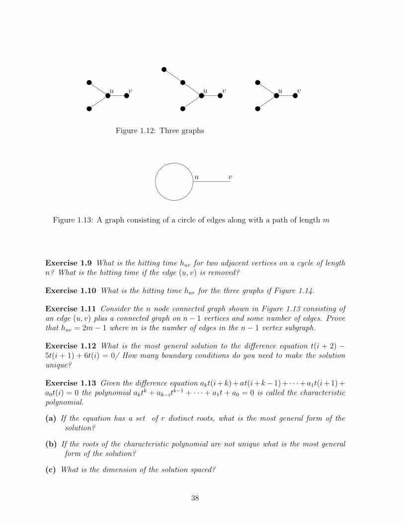
u u uv v v

Figure 1.12: Three graphs

u v

Figure 1.13: A graph consisting of a circle of edges along with a path of length m

Exercise 1.9 What is the hitting time huv for two adjacent vertices on a cycle of lengthn? What is the hitting time if the edge (u, v) is removed?

Exercise 1.10 What is the hitting time huv for the three graphs if Figure 1.14.

Exercise 1.11 Consider the n node connected graph shown in Figure 1.13 consisting ofan edge (u, v) plus a connected graph on n− 1 vertices and some number of edges. Provethat huv = 2m− 1 where m is the number of edges in the n− 1 vertex subgraph.

Exercise 1.12 What is the most general solution to the difference equation t(i + 2) −5t(i + 1) + 6t(i) = 0/ How many boundary conditions do you need to make the solutionunique?

Exercise 1.13 Given the difference equation akt(i+k) +at(i+k− 1) + · · ·+a1t(i+ 1) +a0t(i) = 0 the polynomial akt

k + ak−itk−1 + · · · + a1t + a0 = 0 is called the characteristic

polynomial.

(a) If the equation has a set of r distinct roots, what is the most general form of thesolution?

(b) If the roots of the characteristic polynomial are not unique what is the most generalform of the solution?

(c) What is the dimension of the solution spaced?

38

1 2 3 4

1 2 3 4

1 2 3 4

Figure 1.14: Three graph

(d) If the difference equation is not homogeneous and f(i) is a specific solution to the nonhomogeneous difference equation, what is the full set of solutions to the differenceequation?

Exercise 1.14 Consider the set of integers 1, 2, . . . , n. How many draws d with re-placement are necessary so that every integer is drawn?

Exercise 1.15 Consider a random walk on a clique of size n. What is the expectednumber of steps before a given vertex is reached?

Solution:1n

+ 2 1n(1− 1

n) + 3 1

n(1− 1

n

2) + · · ·

= 1n(1− 1

n)[1 + 2(1− 1

n) + 3(1− 1

n)2 + · · ·

= 1n

[1n

1−(1− 1n

)2

]= 1

n

1− 1n

( 1n

)2

n−1

Exercise 1.16 Show that adding an edge can either increase or decrease hitting time bycalculating h24 for the three graphs in figure 1.14.

Exercise 1.17 Show that adding an edge to a graph can either increase or decrease com-mute time.

Exercise 1.18 Prove that two independent random walks on a two dimensional latticewill hit with probability one.

Exercise 1.19 Consider the lattice in 2-dimensions. In each square add the two diagonaledges. What is the escape probability for the resulting graph?

39

Exercise 1.20 Determine by simulation the escape probability for the 3-dimensional lat-tice.

Exercise 1.21 What is the escape probability for a random walk starting at the root of abinary tree?

Exercise 1.22 Consider a random walk on the positive half line, that is the integers1, 2, 3, . . .. At the origin, always move right one step. At all other integers move rightwith probability 2/3 and left with probability 1/3. What is the escape probability?

Exercise 1.23 What is the probability of returning to the start vertex on a random walkon an infinite planar graph?

Exercise 1.24 Create a model for a graph similar to a 3-dimensional lattice in the waythat a planar graph is similar to a 2-dimensional lattice. What is probability of returningto the start vertex in your model?

Exercise 1.25 Consider a strongly connected directed graph. In the steady state calculatethe flow through each edge of a random walk.

Exercise 1.26 Create a random directed graph with 200 nodes and roughly eight edgesper node. Add k new nodes and calculate the page rank with and without directed edgesfrom the k added nodes to node 1. How much does adding the k edges change the pagerank of nodes for various values of k and restart frequency? How much does adding a loopat node 1 change the page rank? To do the experiment carefully one needs to consider thepage rank of a node to which the star is attached. If it has low page rank its page rank islikely to increase a lot.

Exercise 1.27 Repeat the experiment in Exercise 1.26 for hitting time.

Exercise 1.28 Search engines ignore self loops in calculating page rank. Thus, to increasepage rank one needs to resort to loops of length two. By how much can you increase thepage rank of a page by adding a number of loops of length two?

Exercise 1.29 Can one increase the page rank of a node v in a directed graph by doingsomething some distance from v? The answer is yes if there is a long narrow chain ofnodes into v with no edges leaving the chain. What if there is no such chain?

Exercise 1.30 Consider modifying personal page rank as follows. Start with the uniformrestart distribution and calculate the steady state probabilities. Then run the personalizedpage rank algorithm using the steady state distribution calculated instead of the uniformdistribution. Keep repeating until the process converges. That is, we get a steady stateprobability distribution such that if we use the steady state probability distribution for therestart distribution we will get the steady state probability distribution back. Does thisprocess converge? What is the resulting distribution? What distribution do we get for thegraph consisting of two vertices u and v with a single edge from u to v?

40

Exercise 1.31

(a) What is the hitting time for a vertex in a complete directed graph with self loops?

(b) What is the hitting time for a vertex in a directed cycle with n nodes?

Exercise 1.32 Using a web browser bring up a web page and look at the source html.How would you extract the url’s of all hyperlinks on the page if you were doing a crawlof the web? With Internet Explorer click on “source” under “view” to access the htmlrepresentation of the web page. With Firefox click on “page source” under “view”.

Exercise 1.33 Sketch an algorithm to crawl the World Wide Web. There is a time delaybetween the time you seek a page and the time you get it. Thus, you cannot wait until thepage arrives before starting another fetch. There are conventions that must be obeyed ifone were to actually do a search. Sites specify information has to how long or which filescan be searched. Do not attempt an actual search without guidance from a knowledgeableperson.

Exercise 1.34 Prove Proposition 1.9 that for two probability distributions p,q, |p−q|1 =2∑

i(pi − qi)+.

Exercise 1.35 Suppose S is a subset of at most n2/2 points in the n × n lattice. Showthat

|(i, j) ∈ S : row i, col. j ⊆ S| ≤ |S|/2.

Exercise 1.36 Show that the steady state probabilities of the chain described in the Gibbssampler is the correct p.

Exercise 1.37 A Markov chain is said to be symmetric if for all i and j, pij = pji. Whatis the steady state distribution of a connected aperiodic symmetric chain? Prove youranswer.

Exercise 1.38 How would you integrate a multivariate polynomial distribution over someregion?

Exercise 1.39 Given a time-reversible Markov chain, modify the chain as follows. Atthe current state, stay put (no move) with probability 1/2. With the other probability 1/2,move as in the old chain. Show that the new chain has the same steady state. Whathappens to the convergence time in this modification?

Exercise 1.40 Using the Metropolis-Hasting Algorithm create a Markov chain whose sta-tionary probability is that given in the following table.

x1x2 00 01 02 10 11 12 20 21 22Prob 1/16 1/8 1/16 1/8 1/4 1/8 1/16 1/8 1/16

41

Exercise 1.41 Let p be a probability vector (nonnegative components adding up to 1) onthe vertices of a connected, aperiodic graph. Set pij (the transition probability from i to j)to pj for all i 6= j which are adjacent in the graph. Show that the steady state probabilityvector for the chain is p. Is running this chain an efficient way to sample according to adistribution close to p? Think, for example, of the graph G being the n × n × n × · · ·ngrid.

Exercise 1.42 Construct the edge probability for a three state Markov chain so that thesteady state probability is

(12, 1

3, 1

6

).

Exercise 1.43 Consider a three state Markov chain with steady state probability(

12, 1

3, 1

6

).

Consider the Metropolis-Hastings algorithm with G the complete graph on these threenodes. What is the expected probability that we would actually make a move along aselected edge?

Exercise 1.44 Try Gibbs sampling on p (x) =

(12

00 1

2

).

What happens? How does the Metropolis Hasting Algorithm do?

Exercise 1.45 Consider p(x), where, x = (x1, . . . , x100) and p (0) = 12, p (x) = 1

2100x 6=

0. How does Gibbs sampling behave?

Exercise 1.46 Construct an algorithm and compute the volume of a unit radius spherein 20 dimensions by carrying out a random walk on a 20× 20 grid with 0.1 spacing.

Exercise 1.47 Given a graph G and an integer k how would you generate a sequenceof connected subgraphs S1, S2, . . . of G of size k where Si is generated with probabilityproportional to 2|Ei| where Ei is the set of edges in Si?

Exercise 1.48 What is the mixing time for

(a) a clique?

(b) two cliques connected by a single edge?

Exercise 1.49 Show that for the n× n× · · · × n grid in d space, MEP is Ω(1/dn).Hint: The argument is a generalization of the argument in Exercise 1.35. Argue that forany subset S containing at most 1/2 the grid points, for at least 1/2 the grid points in S,among the d coordinate lines through the point, at least one intersects S.

42